Resource capacity allocation to stochastic dynamic competitors: knapsack problem for perishable items and index-knapsack heuristic

Abstract

In this paper we propose an approach for solving problems of optimal resource capacity allocation to a collection of stochastic dynamic competitors. In particular, we introduce the knapsack problem for perishable items, which concerns the optimal dynamic allocation of a limited knapsack to a collection of perishable or non-perishable items. We formulate the problem in the framework of Markov decision processes, we relax and decompose it, and we design a novel index-knapsack heuristic which generalizes the index rule and it is optimal in some specific instances. Such a heuristic bridges the gap between static/deterministic optimization and dynamic/stochastic optimization by stressing the connection between the classic knapsack problem and dynamic resource allocation. The performance of the proposed heuristic is evaluated in a systematic computational study, showing an exceptional near-optimality and a significant superiority over the index rule and over the benchmark earlier-deadline-first policy. Finally we extend our results to several related revenue management problems.

Appendices

Appendix A: Related revenue management problems

In this section we show in a number of related revenue management problems that the KPPI framework and the results of this paper are of non-trivially wider applicability.

1.1 A.1 Optimal policy to dynamic promotion problem with adaptive knapsack

Consider a retailer for which it is feasible to adjust the promotion space (knapsack) dynamically, e.g. by reserving a necessary number of promotion shelves (or by hiring a necessary number of employees), where given price ν must be paid for each reserved space unit (or for each hired employee). In other words, we assume existence of a space market, where it is permitted to “buy” from other periods some amount of space if necessary or to “sell” to other periods some amount of space if it is not used. Suppose the retailer has allocated a money budget for such a purpose, whose present value is $\widetilde{ W }$. We assume that such a present value was calculated using a discount factor β arising in the perfectly competitive market (i.e., money can be borrowed or lent for the same inter-period interest rate equal (1−β)/β).

Notice that this problem is in fact formulated by (LR^ν). Indeed, the term νW/(1−β) in (LR^ν) can be understood as the present value of a regular money budget (νW per period) allocated for the knapsack space expected to be spent over an infinite horizon. That is, we only need to set $\widetilde{ W } = \nu W / ( 1 - \beta)$. Due to the mutual independence of the products’ demand, the single-item optimal policies from Sect. 5 can be coupled together and we obtain an optimal policy to this multi-product problem.

Proposition 4

Under Assumption 1 satisfied by each product, an optimal policy to the dynamic promotion problem with adaptive knapsack is to buy in every period the promotion space units necessary for promoting all the products whose current index value is greater than ν.

1.2 A.2 Dynamic product assortment problem

Consider the dynamic product assortment problem, in which a retailer wants to choose a collection of products to be displayed for purchase out of all the products available in the retailers’ warehouse. The framework of this paper covers a simple variant of the product assortment problem, in which there is a single unit of each product available from producers. Notice that now the knapsack capacity is given by the total selling space available in the store, and the possible actions for each product is whether to include it in the assortment (action a=1) or not (a=0). Of course, the products not included in the assortment cannot be sold, i.e., q _i :=1 for all products i.

Expression (3) then clearly applies to this problem, and moreover, it simplifies interestingly in the undiscounted case.

Proposition 5

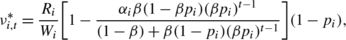
In the dynamic product assortment problem the index value for state $t \in\mathcal{T}_{ i }$ is

• (i) if β<1, p<1, and α _i ≤0, then

  

• (ii) if β=1, p<1, and α _i ≤1, then

  

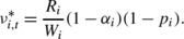
Recall that only products included in the assortment can be sold, and this happens with probability 1−p _i in every period. Interpreting this probability as a service rate μ _i :=1−p _i , the undiscounted index value reduces to cμ, well-known in queuing theory (see, e.g., Smith 1956; Buyukkoc et al. 1985), where the cost c _i :=R _i (1−α _i )/W _i is the revenue loss per unit of space occupied if item is not sold during its lifetime. We emphasize that such an index is constant over time, i.e., it does not depend on the product lifetime.

The cμ-rule prescribes that products should be ordered (highest first) accordingly to the product of their profitability c and per-period attractiveness μ, and included in the assortment following such an ordering. The experimental results from the previous section suggest that IK heuristic may further give an improved solution than the straightforward cμ-index ordering in the case that space requirements W _i are not equal across all the products.

1.3 A.3 Dynamic product pricing problem

Consider a single product and suppose that we are given an additional parameter called discount (price markdown) D _i ≥0, so that the revenue (profit margin) is R _i −D _i instead of R _i if item i is promoted. Thus, 1−q _i can be interpreted as the probability of selling the item priced at R _i , and 1−p _i can be interpreted as the probability of selling the item priced at R _i −D _i . Let a real-valued $\widetilde{ \nu}_{ i }$ be the per-period cost of maintaining (or informing about) the price markdown of this product; thus $\widetilde{ \nu}_{ i } = 0$ may be reasonable in many practical cases. We are then addressing a simple variant of the classic dynamic product pricing problem.

In particular, in the dynamic product pricing problem we have the following expected one-period revenues for $t \in\mathcal{T}_{ i } \setminus\{ 1 \}$:

Denote by $\widetilde{ D }_{ i } := D_{ i } ( 1 - p_{ i } )$. In order to recover the expected one-period revenues under action 1 from the KPPI framework of Sect. 2, we must define the expected one-period revenue for all $t \in\mathcal{T}_{ i }$ as $R_{ i, t }^{ 1 } := \widetilde{ R}_{ i, t }^{ 1 } + \widetilde{ D }_{ i }$. Let us further define the promotion cost $\nu := ( \widetilde{ \nu}_{ i } + \widetilde{ D }_{ i } ) / W_{ i }$. Then, the expected one-period net revenue under action 1 is $R_{ i, t }^{ 1 } - \nu W_{ i, t }^{ 1 } = \widetilde{ R}_{ i, t }^{ 1 } + \widetilde{ D }_{ i } - ( \widetilde{ \nu}_{ i } + \widetilde{ D }_{ i } ) = \widetilde{ R}_{ i, t }^{ 1 } - \widetilde{ \nu}_{ i }$ as desired in the dynamic product pricing model. Then by the definition of indexability we have the following result.

Proposition 6

Suppose that the problem defined above satisfies Assumption 1 and let $\nu_{ i, t }^{ * }$ be the index values given by Theorem 2. Then in the dynamic product pricing problem the following holds for state $t \in\mathcal{T}_{ i }$:

• (i) if $\nu_{ i, t }^{ * } W_{ i } - \widetilde{ D }_{ i } \ge\widetilde{ \nu}_{ i }$, then it is optimal to offer the item with price markdown in state t, and

• (ii) if $\nu_{ i, t }^{ * } W_{ i } - \widetilde{ D }_{ i } \le\widetilde{ \nu}_{ i }$, then it is optimal to offer the item without price markdown in state t.

1.4 A.4 Loyalty card problem

Consider now the multi-product problem like the one addressed in Capgemini and Cisco (2005), in which retailer can use customer’s loyalty card to inform and influence her by personalized messages, say at the moment of arrival to the store. Suppose that the retailer wants to offer the customer a number of products with personalized price markdowns so that the total offered markdown in not larger than a budget D associated with the customer (such a budget could be a function of the customer’s historical expenditures, collected “points”, or any other relevant measure). Of course, now the probabilities p _i and q _i must be the probabilities of buying product i by the customer in hand (say, estimated using the customer’s historical purchasing decisions).

Suppose that every product satisfies Assumption 1. Using the results of the previous subsection, suppose that $\widetilde{ \nu }_{ i } = 0$ and define the knapsack-problem rewards $\widetilde{ v }_{ i } := \nu_{ i, t }^{ * } W_{ i } - \widetilde{ D }_{ i }$. Then, analogously to the arguments given in Sect. 6, we propose to use the solution to the following 0–1 knapsack subproblem in step (iv) of the IK heuristic for the loyalty card problem:

where $\boldsymbol{z}= ( z_{ i } : i \in\mathcal{I})$ is the vector of binary decision variables denoting whether each item i is offered with price markdown or not.

Appendix B: Preliminaries of work-revenue analysis

In order to prove Theorem 2, we describe the key points from the restless bandit framework in more detail. For a survey on this methodology we refer to Niño-Mora (2007b). We can restrict our attention to stationary deterministic policies, since it is well-known from the MDP theory that there exists an optimal policy which is stationary, deterministic, and independent of the initial state. Notice that any set $\mathcal{S}\subseteq\mathcal{T}$ can represent a stationary policy, by employing action 1 in all the states belonging to $\mathcal{S}$ and employing action 0 in all the states belonging to $\mathcal{T}\setminus\mathcal{S}$. We will call such a policy an $\mathcal{S}$-active policy, and $\mathcal{S}$ an active set.

Let $\mathcal{S}\subseteq\mathcal{T}$ be an active set. We can reformulate (1) as

(9)

where $\boldsymbol{P}_{ i, j }^{ j - i | \mathcal{S}}$ is the probability of moving from state $i \in\mathcal{X}$ to state $j \in\mathcal{X}$ in exactly j−i periods under policy $\mathcal{S}$ and $I_{\mathcal{S}} ( s )$ is the indicator function

$$I_{ \mathcal{S}} ( s ) = \begin{cases} 1, & \text{ if } s \in\mathcal{S}, \\ 0, & \text{ if } s \notin\mathcal{S}. \end{cases} $$

So, $\mathbb{R}_{ t }^{ \mathcal{S}}$ is the expected total discounted revenue under policy $\mathcal{S}$ if starting from state t, and we will write it in a more convenient way as

(10)

Similarly, $\mathbb{W}_{ t }^{ \mathcal{S}}$ is the expected total discounted promotion work under policy $\mathcal{S}$ if starting from state t, and we will write it in a more convenient way as

(11)

Let, further, $\langle a, \mathcal{S}\rangle$ be the policy which takes action $a \in\mathcal{A}$ in the current time period and adopts an $\mathcal{S}$-active policy thereafter. For any state $t \in\mathcal{T}$ and an $\mathcal{S}$-active policy, the $( t, \mathcal{S})$-marginal revenue is defined as

$$ r_{ t }^{ \mathcal{S}} := \mathbb{R}_{ t }^{ \langle1, \mathcal {S}\rangle} - \mathbb{R}_{ t }^{ \langle0, \mathcal{S}\rangle}, $$

(12)

and the $( t, \mathcal{S})$-marginal promotion work as

$$ w_{ t }^{ \mathcal{S}} := \mathbb{W}_{ t }^{ \langle1, \mathcal {S}\rangle} - \mathbb{W}_{ t }^{ \langle0, \mathcal{S}\rangle}. $$

(13)

These marginal revenue and marginal promotion work capture the change in the expected total discounted revenue and promotion work, respectively, which results from being active instead of passive in the first time period and following the $\mathcal{S}$-active policy afterwards. Finally, if $w_{ t }^{ \mathcal{S}} \neq0$, we define the $( t, \mathcal{S})$-marginal promotion rate as

$$ \nu_{ t }^{ \mathcal{S}} := \frac{ r_{ t }^{ \mathcal{S}} }{ w_{ t }^{ \mathcal{S}} }. $$

(14)

Let us consider a family of nested sets $\mathcal{F}:= \{ \mathcal {S}_{ 0 }, \mathcal{S}_{ 1 }, \dots, \mathcal{S}_{ T } \}$, where $\mathcal {S}_{ k } := \{ 1, 2, \dots, k \}$. We will use the following theorem to establish indexability and obtain the index values.

Theorem 4

(Niño-Mora 2002)

If problem (1) satisfies the following two conditions (so-called PCL($\mathcal{F}$)-indexability):

• (i) the marginal promotion work $w_{ t }^{ \mathcal{S}} > 0$ for all $t \in\mathcal{T}$ and for all $\mathcal{S}\in\mathcal {F}$, and

• (ii) the marginal promotion rate $\nu_{ t }^{ \mathcal{S}_{ t - 1 } }$ is nonincreasing in $t \in\mathcal{T}$,

then the problem is indexable, family $\mathcal{F}$ contains an optimal active set for any value of parameter ν, and the index values are $\nu_{ t }^{ * } := \nu_{ t }^{ \mathcal{S}_{ t - 1 } }$ for all $t \in \mathcal{T}$.

Appendix C: Proof of Theorem 2

The ultimate goal of the proof is to apply Theorem 4 and derive a closed-form expression for the index given in Theorem 2. Plugging (10) and (11) into (12) and (13), respectively, we obtain two expressions that will be used in the following analysis:

(15)

(16)

It is well known in the MDP theory that the transition probability matrix for multiple periods is obtained by multiplication of transition probability matrices for subperiods. Hence, given an active set $\mathcal{S} \subseteq\mathcal{T}$, we have

$$ \boldsymbol{P}^{ t - s | \mathcal{S}} = \bigl( \boldsymbol{P}^{ 1 | \mathcal{S}} \bigr)^{ t - s }, $$

(17)

where the matrix $\boldsymbol{P}^{ 1 | \mathcal{S}}$ is an (T+1)×(T+1)-matrix constructed so that its row $x \in\mathcal{X}$ is the row x of the matrix $\boldsymbol{P}^{ 1 | \mathcal{T}}$ if $x \in \mathcal{S}$, and is the row x of the matrix P ^1|∅ otherwise. For definiteness, we remark that $\boldsymbol{P}^{ 0 | \mathcal{S}}$ is an identity matrix.

We will use the following characterization of the marginal measures.

Lemma 1

Let $t \in\mathcal{T}$ and consider any integer 0≤k≤T. Then,

(18)

(19)

Proof

Under an active set $\mathcal{S}_{ k }$, from (17) we get for T≥t−1≥s≥1,

These expressions together with the definitions of $R_{ t }^{ a }$ and $W_{ t }^{ a }$ plugged into (15)–(16) after simplification conclude the proof. □

The following lemma establishes condition (i) of PCL($\mathcal {F}$)-indexability.

Lemma 2

For any integer k≥0 we have

• (i) $w_{ k }^{ \mathcal{S}_{ k } } > 0$;

• (ii) $w_{ t }^{ \mathcal{S}_{ k } } > 0$ for all $t \in \mathcal{T}$.

Proof

Denote by

(20)

so that, using (19), $w_{ k }^{ \mathcal{S}_{ k } } = W [ 1 - h ( k ) ]$.

• (i) For k=0, we have h(0)=0 by definition. For k≥1, $h ( k ) = ( 1 - ( \beta p )^{ k } ) \frac{ \beta q - \beta p }{ 1 - \beta p } < 1$.

• (ii) Implied by (i) and (19).

 □

Next we establish condition (ii) of $\mathrm{PCL}(\mathcal{F})$-indexability.

Lemma 3

We have

Moreover, under Assumption 1, $\nu_{ t }^{ \mathcal {S}_{ t - 1 } }$ is nonincreasing in $t \in\mathcal{T}$.

Proof

Consider $\mathcal{S}_{ t - 1 }$ for $t \in\mathcal{T}$. By Lemma 1 we have

therefore

(21)

After multiplying both the numerator and the denominator by 1−βp, and rearranging the terms, we obtain

By Assumption 1, (1−q)−α(1−βq)≥0 and q−p>0, therefore $\nu_{ t }^{ \mathcal{S}_{ t - 1 } }$ is nonincreasing in t. □

Finally, we can apply Theorem 4 to conclude that under Assumption 1, the problem is indexable and the index values are given by $\nu_{ t }^{ \mathcal{S}_{ t - 1 } }$ in Lemma 3, which also establishes the time monotonicity.  □

Appendix D: Proof of Proposition 1

• (i) Immediate from (21).

• (ii) Formally, we are to prove the following statement: If the probability q is replaced by q′≤q, then $\nu_{ t }^{ * \prime} \le\nu_{ t }^{ * }$ for any $t \in \mathcal{T}$. It is straightforward to see that (21) is nondecreasing in q. □

References

Anselmi, J., & Verloop, I. M. (2011). Energy-aware capacity scaling in virtualized environments with performance guarantees. Performance Evaluation, 68, 1207–1221.
Burnetas, A. N., & Katehakis, M. N. (1998). Dynamic allocation policies for the finite horizon one armed bandit problem. Stochastic Analysis and Applications, 16(5), 811–824.
Burnetas, A. N., & Katehakis, M. N. (2003). Asymptotic Bayes analysis for the finite horizon one armed bandit problem. Probability in the Engineering and Informational Sciences, 17(1), 53–82.
Buyukkoc, C., Varaiya, P., & Walrand, J. (1985). The cμ rule revisited. Advances in Applied Probability, 17(1), 237–238.
Capgemini, I., & Cisco, M. (2005). Retailers transform processes with ERS. In M. Hann (Ed.), RetailSpeak. www.retailspeak.com.
Caro, F., & Gallien, J. (2007). Dynamic assortment with demand learning for seasonal consumer goods. Management Science, 53(2), 276–292.
Chick, S. E., & Gans, N. (2009). Economic analysis of simulation selection problems. Management Science, 55(3), 421–437.
Dance, C., & Gaivoronski, A. A. (2012). Stochastic optimization for real time service capacity allocation under random service demand. Annals of Operations Research, 193, 221–253. doi:10.1007/s10479-011-0842-2.
Dantzig, G. B. (1957). Discrete-variable extremum problems. Operations Research, 5(2), 266–277.
Elmaghraby, W., & Keskinocak, P. (2003). Dynamic pricing in the presence of inventory considerations: research overview, current practices, and future directions. Management Science, 49(10), 1287–1309.
Gesbert, D., Kountouris, M., Health, R. W. J., Chae, C. B., & Sälzer, T. (2007). Shifting the MIMO paradigm. IEEE Signal Processing Magazine, 36, 36–46.
Gittins, J. C. (1979). Bandit processes and dynamic allocation indices. Journal of the Royal Statistical Society, Series B, 41(2), 148–177.
Gittins, J. C., & Jones, D. M. (1974). A dynamic allocation index for the sequential design of experiments. In J. Gani (Ed.), Progress in statistics (pp. 241–266). Amsterdam: North-Holland.
Glazebrook, K., & Minty, R. (2009). A generalized Gittins index for a class of multiarmed bandits with general resource requirements. Mathematics of Operations Research, 34(1), 26–44.
Glazebrook, K. D., Mitchell, H. M., & Ansell, P. S. (2005). Index policies for the maintenance of a collection of machines by a set of repairmen. European Journal of Operational Research, 165, 267–284.
Glazebrook, K. D., Hodge, D. J., & Kirkbride, C. (2011). General notions of indexability for queueing control and asset management. Annals of Applied Probability, 21, 876–907.
Jacko, P. (2010). Restless bandits approach to the job scheduling problem and its extensions. In A. B. Piunovskiy (Ed.), Modern trends in controlled stochastic processes: theory and applications (pp. 248–267). United Kingdom: Luniver Press.
Jacko, P. (2011a). Optimal index rules for single resource allocation to stochastic dynamic competitors. In Proceedings of ValueTools, ACM Digital Library.
Jacko, P. (2011b). Value of information in optimal flow-level scheduling of users with Markovian time-varying channels. Performance Evaluation, 68(11), 1022–1036.
Katehakis, M. N., & Derman, C. (1987). Computing optimal sequential allocation rules in clinical trials. In J. V. Ryzin (Ed.), I.M.S. lecture notes-monograph series: Vol. 8. Adaptive statistical procedures and related topics (pp. 29–39).
Katehakis, M. N., & Veinott, A. F. (1987). The multi-armed bandit problem: decomposition and computation. Mathematics of Operations Research, 12(2), 262–268.
Loch, C. H., & Kavadias, S. (2002). Dynamic portfolio selection of NPD programs using marginal returns. Management Science, 48(10), 1227–1241.
Manor, G., & Kress, M. (1997). Optimality of the greedy shooting strategy in the presence of incomplete damage information. Naval Research Logistics, 44, 613–622.
Meuleau, N., Hauskrecht, M., Kim, K. E., Peshkin, L., Kaelbling, L. P., Dean, T., & Boutilier, C. (1998). Solving very large weakly coupled Markov decision processes. In Proceedings of the fifteenth national conference on artificial intelligence (pp. 165–172).
Niño-Mora, J. (2001). Restless bandits, partial conservation laws and indexability. Advances in Applied Probability, 33(1), 76–98.
Niño-Mora, J. (2002). Dynamic allocation indices for restless projects and queueing admission control: a polyhedral approach. Mathematical Programming, Series A, 93(3), 361–413.
Niño-Mora, J. (2005). Marginal productivity index policies for the finite-horizon multiarmed bandit problem. In Proceedings of the 44th IEEE conference on decision and control and European control conference ECC 2005 (CDC-ECC’05) (pp. 1718–1722).
Niño-Mora, J. (2007a). A (2/3)n 3 fast-pivoting algorithm for the Gittins index and optimal stopping of a Markov chain. INFORMS Journal on Computing, 19(4), 596–606.
Niño-Mora, J. (2007b). Dynamic priority allocation via restless bandit marginal productivity indices. TOP, 15(2), 161–198.
Papadimitriou, C. H., & Tsitsiklis, J. N. (1999). The complexity of optimal queueing network. Mathematics of Operations Research, 24(2), 293–305.
Pisinger, D. (2005). Where are the hard knapsack problems? Computers & Operations Research, 32, 2271–2284.
Qu, S., & Gittins, J. C. (2011). A forwards induction approach to candidate drug selection. Advances in Applied Probability, 43(3), 649–665.
Smith, W. E. (1956). Various optimizers for single-stage production. Naval Research Logistics Quarterly, 3(1–2), 59–66.
Speitkamp, B., & Bichler, M. (2010). A mathematical programming approach for server consolidation problems in virtualized data centers. IEEE Transactions on Services Computing, 3(4), 266–278.
Varaiya, P., Walrand, J., & Buyukkoc, C. (1985). Extensions of the multiarmed bandit problem: the discounted case. IEEE Transactions on Automatic Control, AC-30(5), 426–439.
Weber, R., & Weiss, G. (1990). On an index policy for restless bandits. Journal of Applied Probability, 27(3), 637–648.
Whittle, P. (1981). Arm-acquiring bandits. Annals of Probability, 9(2), 284–292.
Whittle, P. (1988). Restless bandits: activity allocation in a changing world. A celebration of Applied Probability. Journal of Applied Probability, 25A, 287–298. J. Gani (Ed.).
Yang, R., Bhulai, S., & van der Mei, R. (2011). Optimal resource allocation for multiqueue systems with a shared server pool. Queueing Systems, 68, 133–163.
Author information
Authors and Affiliations
Corresponding author
Additional information
An earlier version of this paper was presented at the BCAM Workshop on Bandit Problems (Bilbao, 2011) and at the INFORMS Applied Probability Society Conference (Stockholm, 2011). Research partially supported by grant MTM2010-17405 of the MICINN (Spain) and grant SA-2012/00331 of the Department of Industry, Innovation, Trade and Tourism (Basque Government).