On-line estimators for ad-hoc task execution: learning types and parameters of teammates for effective teamwork

Abstract

It is essential for agents to work together with others to accomplish common objectives, without pre-programmed coordination rules or previous knowledge of the current teammates, a challenge known as ad-hoc teamwork. In these systems, an agent estimates the algorithm of others in an on-line manner in order to decide its own actions for effective teamwork. A common approach is to assume a set of possible types and parameters for teammates, reducing the problem into estimating parameters and calculating distributions over types. Meanwhile, agents often must coordinate in a decentralised fashion to complete tasks that are displaced in an environment (e.g., in foraging, de-mining, rescue or fire control), where each member autonomously chooses which task to perform. By harnessing this knowledge, better estimation techniques can be developed. Hence, we present On-line Estimators for Ad-hoc Task Execution (OEATE), a novel algorithm for teammates’ type and parameter estimation in decentralised task execution. We show theoretically that our algorithm can converge to perfect estimations, under some assumptions, as the number of tasks increases. Additionally, we run experiments for a diverse configuration set in the level-based foraging domain over full and partial observability, and in a “capture the prey” game. We obtain a lower error in parameter and type estimation than previous approaches and better performance in the number of completed tasks for some cases. In fact, we evaluate a variety of scenarios via the increasing number of agents, scenario sizes, number of items, and number of types, showing that we can overcome previous works in most cases considering the estimation process, besides robustness to an increasing number of types and even to an erroneous set of potential types.

1 Introduction

Autonomous agents are usually designed to pursue a specific strategy and accomplish a single or set of tasks. Intending to improve their performance, these agents often follow specified coordination and communication protocols to enable the collection of valuable information from the environment components or even from other reliable agents. However, employing these methods is challenging due to environmental and technological constraints. There are circumstances where communication channels are unreliable, and agents cannot fully trust them to send or receive information. Moreover, particular situations require the design of agents (e.g., robots or autonomous systems) from various parties aiming to solve a problem urgently, but constructing and testing communication and coordination protocols for all different agents can be unfeasible given the time constraints. For example, consider a natural disaster or a hazardous situation where institutions may urgently ship robots from different parts of the world for handling the problem. In these scenarios, avoiding delays and unnecessary funding usage would save lives and mitigate the caused damages

One possible solution is to offer a centralised mechanism to allocate tasks to each agent in the environment in an efficient manner. However, we may face scenarios where there is no centralised mechanism available to manage the agents’ actions. When we consider large scale problems, it is even easier to imagine situations where environmental or time constraints also derail this solution. Hence, agents need to decide, autonomously, which task to pursue [11]—defining what we will denominate a decentralised execution scenario. The decentralised execution is quite natural in ad-hoc teamwork, as we cannot assume that other agents would be programmed to follow a centralised controller. Therefore, allowing agents to reason about the surrounding environment and create partnerships with other agents can support the accomplishment of missions that are hard to deal with individually, reducing the necessary time to achieve all tasks and minimising the costs related to the process.

For many relevant domains, these decentralised execution problems can be modelled focused on the set of tasks that need to be accomplished in a distributed fashion (e.g., victims to be rescued from a hazard, letters to be quickly delivered to different locations, etc). Note this kind of design presents a task-based perspective to solve the problem, where agents must reason about their teammates’ targets to improve the coordination, hence the team’s performance. In this way, the agents must approximate the teammates’ behaviours (or their main features) in order to deliver this improvement while solving the problem.

As our first goal, this paper will address the problem where agents are supposed to complete several tasks cooperatively in an environment where there is no prior information, reliable communication channel or standard coordination protocol to support the problem completion. We will denominate this ad-hoc team situation as a Task-based Ad-hoc Teamwork problem, a decentralised distributed system where agents decide their tasks autonomously, without previous knowledge of each other, in an environment full of uncertainties.

Instead of developing algorithms that are able to learn any possible policy from scratch, a common approach in the ad-hoc teamwork literature is to consider a set of possible agent types and parameters, thereby reducing the problem of estimating those [2, 3, 10]. This approach is more applicable, as it does not require a large number of observations, thus allows the learning and acting to happen simultaneously in an on-line fashion, i.e., in a single execution. Types could be built based on previous experiences [7, 8] or derived from the domain [1]. Moreover, the introduction of parameters for each type allows more fine-grained models [2]. However, the previous works that learn types and parameters in ad-hoc teamwork are not specifically designed for decentralised task execution, missing an opportunity to obtain better performances in this relevant scenario for multi-agent collaboration.

Other lines of work focus on neural network-based models and learn the policies of other agents after thousands (even millions) of observations [22, 33]. These applications, however, would be costly, especially when domains get larger and more complicated. Similarly, I-POMDP based models [12, 17, 19, 23] could be applied for reasoning about the model of other agents from scratch, but its application is non-trivial considering larger problems.

On the other hand, some approaches in the literature have also tested task-based designs, inferring about agents pursuing tasks to predict their behaviour [13]. Although we share some similarities, they have not yet handled learning types and parameters of agents in ad-hoc teamwork systems where multiple agents may need to cooperate to complete common tasks.

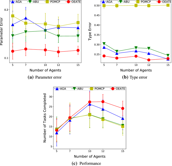
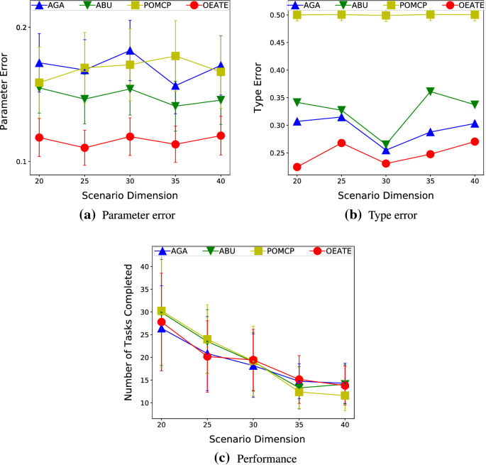
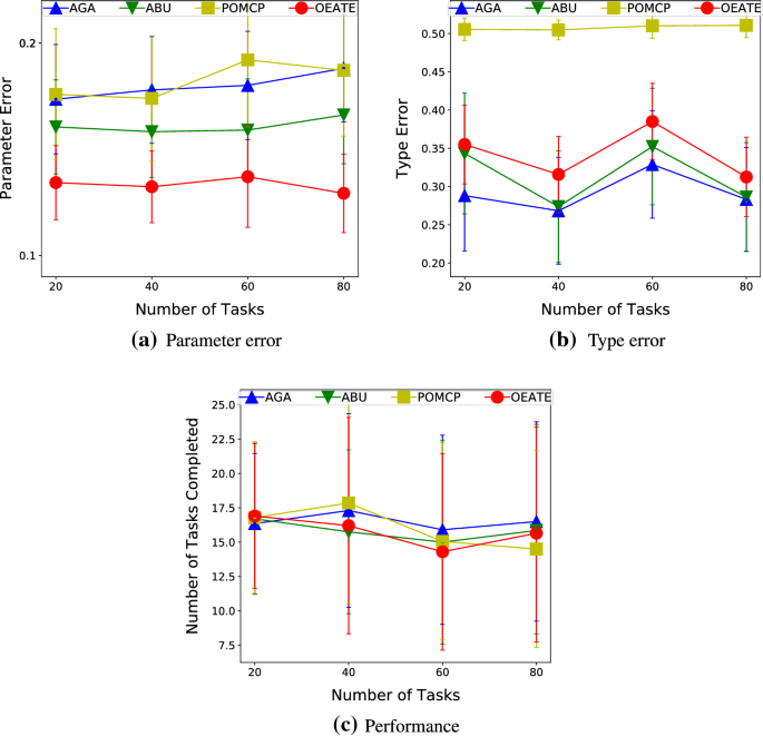
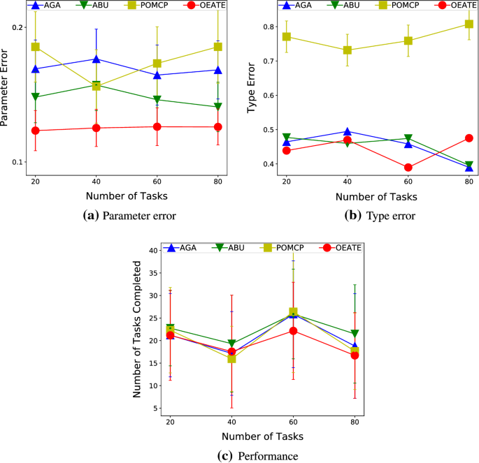
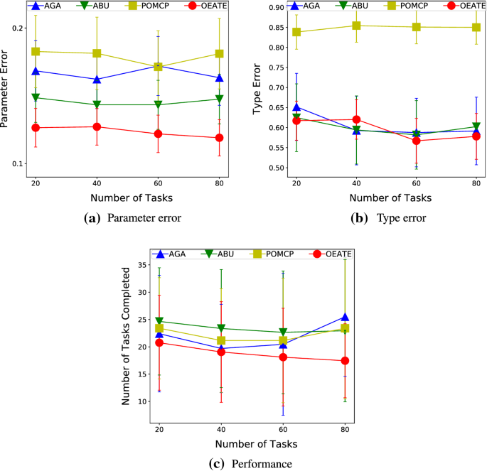
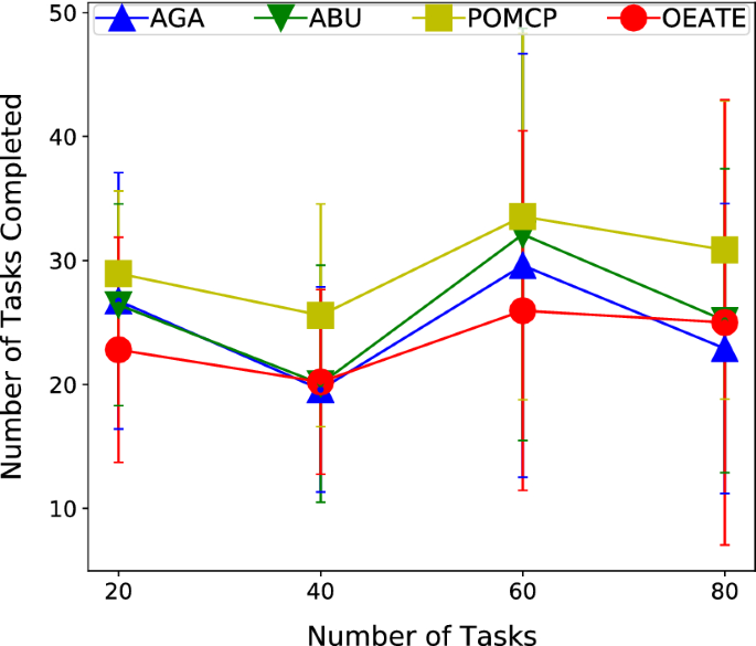
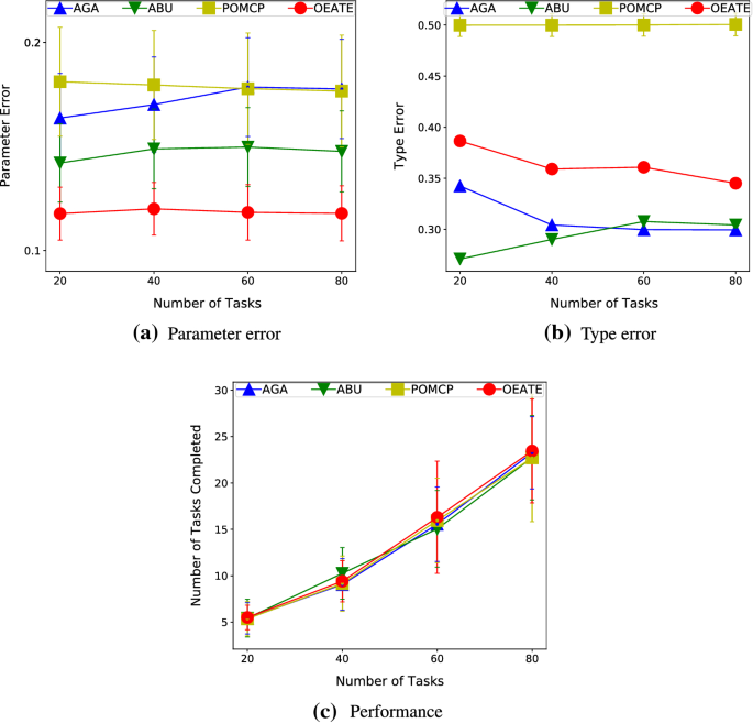
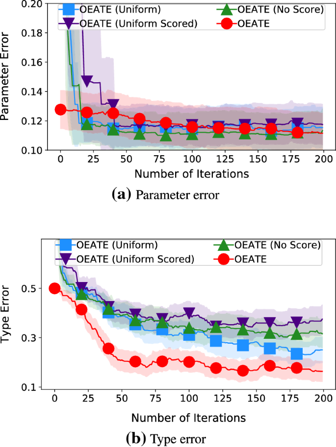
Therefore, as our main contribution, we present in this paper On-line Estimators for Ad-hoc Task Execution (OEATE), a novel algorithm for estimating teammates types and parameters in decentralised task execution. Our algorithm is light-weighted, running estimations from scratch at every single run, instead of employing pre-trained models, or carrying knowledge between executions. Under some assumptions, we show theoretically that our algorithm converges to a perfect estimation when the number of tasks to be performed gets larger. Additionally, we run experiments for two collaborative domains: (ii) a level-based foraging domain, where agents collaborate to collect “heavy” boxes together, and; (ii) a capture the prey domain, where agents must collaborate to surround preys and capture them. We also tested the performance of our method in full and partial observable scenarios. We show that we can obtain a lower error in parameter and type estimations in comparison with the state-of-the-art, leading to significantly better performance in task execution for some of the studied cases. We also run a range of different scenarios, considering situations where the number of agents, scenario sizes, and the number of items gets larger. Furthermore, we evaluate the impact of increasing the number of possible types. Finally, we run experiments where our ad-hoc agent does not have the true type of the other agents in its pool of possible agent types. In such challenging situations, our parameter estimation outstands the competitors and, our type estimation and performance is similar or better than the state-of-the-art in several cases considering the results’ confidence interval.

2 Background

Ad-hoc Teamwork Model Ad-hoc teamwork defines domains where agents intend to cooperate with their teammates and coordinate their actions to reach common goals. Moreover, agents in the domains do not have any prior communication or coordination protocols to enable the exchange of information between them, so learning and reasoning about the current context are mandatory to improve the team’s performance as a unit. However, if agents are aware of some potential pre-existing standards for coordination and communication, they can try to learn about their teammates with limited information [8]. As a result of such intelligent coordination in the ad-hoc teams, they can improve their decision-making process and hence, accomplish shared goals more efficiently.

This fundamental model can be extended to fit many problems and scenarios. For our work, we will extend it to a task-based model, enabling a better representation of our world as presented in previous state-of-the-art works [5, 6, 41].

Task-based Ad-hoc Teamwork Model As an extension of ad-hoc teamwork model, the task-based ad-hoc teamwork model represents a problem where one learning agent $\phi$, acts in the same environment as a set of non-learning agents $\omega \in \varvec{\Omega }$, $\phi \notin \varvec{\Omega }$. In the ad-hoc team $\phi \cup \varvec{\Omega }$, the objective of $\phi$ (as the learning agent) is to maximise the performance (e.g., the number of tasks accomplished or the necessary time to finish them all). However, all non-learning agents’ models are unknown to $\phi$, and there is no communication channel available. Hence, $\phi$ must estimate and understand their models as time progresses, by observing the scenario. In other words, the learning agent must improve its decision-making process by approximating the teammates’ behaviour in an on-line manner and facing a lack of information.

Besides, there is a set of tasks $\mathbf {T}$ which all agents in the team endeavour to accomplish autonomously. A task $\tau \in \mathbf {T}$ may require multiple agents to perform it successfully and multiple time steps to be completed. For instance, in a foraging problem, a heavy item may require two or more robots to be collected, and the robots would need to move towards the task location to accomplish it, taking multiple time steps to move from their initial position.

The learning agent $\phi$ must minimise the time to accomplish all tasks. Hence, playing this role requires the support of a method that integrates the estimation and the decision-making process while performing and improving the planning.

Model of Non-Learning Agents All non-learning agents aim to finish the tasks in the environment autonomously. However, choosing and completing a task $\tau$ by any $\omega$ is dependent on its internal algorithm and its capabilities. Nonetheless, $\omega$’s algorithm can be one of the potential algorithms defined in the system, which might be learned from previous interactions with other agents [7].

Therefore, following the model of Non-Learning agents defined in previous works [2, 41], there is a set of potential algorithms in the system, which compose a set of possible types $\varvec{\Theta }$ for all $\omega \in \varvec{\Omega }$. The assumption is that all these algorithms have some inputs, which is denominated parameters. Hence, the types are all parameterised, which affects agents’ behaviour and actions. Considering the existence of these types’ parameters allows $\phi$ to use more fine-grained models when handling new unknown agents.

According to these assumptions, each $\omega \in \varvec{\Omega }$ will be represented by a tuple ($\theta$, $\mathbf {p}$), where $\theta \in \varvec{\Theta }$ is $\omega$’s type and $\mathbf {p}$ represents its parameters, which is a vector $\mathbf {p} = <p_1,p_2,\ldots ,p_n>$. Also, each element $p_i$ in the vector $\mathbf {p}$ is defined in a fixed range [$p_i^{min}$, $p_i^{max}$] [2]. So, the whole parameter space can be represented as $\mathbf {P} \subset \mathbb {R}^{n}$. These parameters can be the abilities and skills of an agent. For instance, a robot can be quite different depending on its hardware—for a robot, it can be vision radius, the maximum battery level or the maximum velocity. The parameters could also be hyper-parameters of the algorithm itself. Consequently, each $\omega \in \varvec{\Omega }$, based on its type $\theta$ and parameters $\mathbf {p}$, will choose a target task. The process of choosing a new task can happen at any time and any state in the state space, depending on the agents’ parameters and type. We denominate these decision states as Choose Target States $\mathfrak {s} \in S$.

In the Task-based Ad-hoc Teamwork context, a precise estimation of tasks also depends on estimating the Choose Target State. Our method presents a solution to this problem by considering an information-based perspective, which does its evaluation by giving different weights to the information derived from observations made by the agent $\phi$, instead of directly estimating the choose target state. More detail will be presented in Sect. 6.

Stochastic Bayesian Game Model A Stochastic Bayesian Game (SBG) describes a well-suited solution towards the representation of ad-hoc teamwork problems that combine the Bayesian games with the concept of stochastic games and provide a descriptive model to the context [4, 29]. In this section, we will define an SBG-based model for our specific setting and refer the reader to [29] for a more generic formulation.

Our model consists of a discrete state space S, a set of players ($\phi \cup \varvec{\Omega }$), a state transition function $\mathcal {T}$ and a type distribution $\Delta$. Each agent $\omega \in \varvec{\Omega }$ has a type $\theta _i \in \varvec{\Theta }$ and a parameter space $\mathbf {P}$. Each parameter is a vector $\mathbf {p} = <p_1,p_2 \ldots p_n>$ and each $p_i \in [p_i^{min},p_i^{max}]$, for all agents. The set $[p_1^{min},p_1^{max}] \times \dots \times [p_n^{min},p_n^{max}] = \mathbf {P} \subset \mathbb {R}^n$ is the parameter space for each agent. Each type could have a different parameter space, but we define a single parameter space here for simplicity of notation. Furthermore, we assume that the types of the agents are fixed throughout the process (a pure and static type distribution). Moreover, each player is associated with a set of actions, an individual payoff function and a strategy. Considering that at each time step, agents $\omega _i \in \varvec{\Omega }$ are fixed tuples $(\theta _i, \mathbf {p}_i)$, where $\theta _i \in \varvec{\Theta }$ and $\mathbf {p}_i \in \mathbf {P}$, we extend the SBG model in order to describe the following problem:

Problem Consider a set of players $\phi \cup \varvec{\Omega }$ that share the same environment. Each player acts according to its type $\theta _i$, set of parameters $\mathbf {p}_i$ and own strategy $\pi _i$. They do not know the others’ types or parameters. At each time step t, given the state $s^t$ and a joint action $a^t = (a^t_\phi ,a^t_1,a^t_2,\ldots ,a^t_{|\varvec{\Omega }|})$, the game transitions accordingly to the transition probability $\mathcal {T}$ and each player receives an individual payoff $r_i$ until the game reaches a terminal state.

Therefore, by using the SBG model, we can represent our problem and the necessary components in it. However, we consider in this work a fully cooperative problem, under the point of view of agent $\phi$. Hence, within the task-based ad-hoc teamwork context, we want to model the problem employing a single-player abstraction under $\phi$’s point of view. Using a Markov Decision Process Model (MDP), we can abstract all the environment components as part of the state (including teammates in $\varvec{\Omega }$). This approach enables the aggregation of individual rewards from the SBG model into a single global reward and allows us to use single-player Monte Carlo Tree Search techniques, as previous works did [5, 32, 41].

Markov Decision Process Model The Markov Decision Process (MDP) consists of a mathematical framework to model stochastic processes in a discrete time flow. As mentioned, although there are multiple agents and perspectives in the team, we will define the model considering the point of view of an agent $\phi$ and apply a single agent MDP model, as in previous works [5, 32, 41] that represent other agents as part of the environment.

Therefore, we consider a set of states $s \in \mathcal {S}$, a set of actions $a \in \mathcal {A}_\phi$, a reward function $\mathcal {R}(s,a)$, and a transition function $\mathcal {T}$, where the actions in the model are only the $\phi$’s actions. In other words, $\phi$ can only decide its own actions and has no control over other environment components (e.g., actions of agents in the set $\varvec{\Omega }$). All $\omega$ in $\varvec{\Omega }$ are modelled as the environment, as their actions indirectly affect the next state and the obtained reward. Therefore, they are abstracted in the transition function. That is, in the actual problem, the next state depends on the actions of all agents, however, $\phi$ is unsure about the non-learning agents next action. For this reason, we consider that given a state s, an agent $\omega \in \varvec{\Omega }$ has a (unknown) probability distribution (pdf) across a set of actions $\mathcal {A}_{\omega }$, which is given by $\omega$’s internal algorithm ($\theta$, $\mathbf {p}$). This pdf is going to affect the probability of the next state. Therefore, we can say that the uncertainty in the MDP model comes from the randomness of the actions of the $\omega$ agents, besides any additional stochasticity of the environment.

This model allows us to employ single-agent on-line planning techniques, like UCT Monte Carlo Tree Search [26]. In the tree search process, the pdf of each agent defines the transition function. At each node transition, $\phi$ samples $\omega$ agents’ actions from their (estimated) pdfs, and that will determine the next state $s'$ for the next node. However, in traditional UCT Monte Carlo Tree Search, the search tree increases exponentially with the number of agents. Hence, we use a history-based version of UCT Monte Carlo Tree Search called UCT-H, which employs a more compact representation than the original algorithm, and helps to trace the tree in larger teams in a simpler and faster fashion [41].

As mentioned earlier, in this task-based ad-hoc team, $\phi$ attempts to help the team to get the highest possible reward. For this reason, $\phi$ needs to find the optimal value function, which maximises the expected sum of discounted rewards $E[\sum _{j=0}^{\infty }\gamma ^jr_{t+j}]$, where t is the current time, $r_{t+j}$ is the reward $\phi$ receives at j steps in the future, $\gamma \in (0, 1]$ is a discount factor. Also, we consider that we obtain the rewards by solving the tasks $\tau \in \mathbf {T}$. That is, we define $\phi$’s reward as $\sum r(\tau )$, where $r(\tau )$ is the reward obtained after the task $\tau$ completion. Note that the sum of rewards is not only across the tasks completed by $\phi$, but all tasks completed by any set of agents in a given state. Furthermore, there might be some tasks in the system that cannot be completed without cooperation between the agents, so the number of required agents for finishing a task $\tau$ depends on each specific task and the set of agents that are jointly trying to complete it.

Note that the agents’ types and parameters are actually not observable, but in our MDP model that is not directly considered also. Estimated types and parameters are used during on-line planning, creating an estimated transition function. The actual decisions made by the non-learning agents is observable in the real world transitions without any direct information about type and parameters. More details are available in the next section.

3 Related works

The literature introduces ad-hoc teamwork as a remarkable approach to handle multi-agents systems [5, 38]. This approach presents the opportunity to achieve the objectives of the multiple agents in a collaborative manner that surpasses the requirement of designing a communication channel for information exchanging between the agents, building an application to do prior coordination or the collection of previous data that train agents intending to improve the decision-making process within the environment. Furthermore, these models enable the creation of algorithms capable of acting in an on-line fashion, dynamically adapting their behaviour according to the environment and current teammates.

In this section, we will carry out a comprehensive discussion about the state-of-the-art contributions and how these different approaches have inspired our work. Intending to facilitate understanding and readability, we organised the section into topics and related contributions by groups. Each subsection categorises the major idea of each group and summarises the main strategy of those.

3.1 Type-based parameter estimation

Considering type-based reasoning and parameters learning, we can solve the problem using fine-grained models, which evaluate the observations and estimate each agent’s type and parameters in an on-line manner [1, 3, 7, 8, 10]. These lines of works propose the approximation of agents’ behaviour to a set of potential types to improve the ad-hoc agents’ decision-making capabilities, allowing a quick on-line estimation of agents’ algorithms, without requiring an expensive training process for learning their policies from scratch. However, if a set of potential types and the parameter space cannot be defined through domain knowledge, then they would have to be learned from previous interactions [8].

Albrecht and Stone [2], in particular, introduced the AGA and ABU algorithms for type-based reasoning of teammates parameters in an on-line manner, which are the main inspirations for this work. Both methods sample sets of parameters (from a defined parameter space) to perform estimations via gradient ascent and Bayesian updates, respectively. However, by focusing on decentralised task execution in ad-hoc teams, our novel method surpasses their parameter and type estimations when the number of teammates gets larger or more tasks are accomplished, consequently leading to better team performance. We also extend their work by adding partial observability to all team members.

On the other hand, Hayashi et al. [22] propose an enhanced particle reinvigorating process that leverages prior experiences encoded in a recurrent neural network (RNN), acting into a partial observable scenario in their ad-hoc team. However, they need thousands of previous experiences for training the RNN, while still requiring knowledge of the potential types. Our approach can start from scratch at every single run, with no pre-training.

Concerning problems with partial observability, POMCP is usually employed for on-line planning [37]. However, it is originally designed for a discrete state space, making it harder to apply POMCP for (continuous) parameter estimation. However, we apply POMCP in combination with our algorithm OEATE, which enables the decision making on partial observable scenarios and improves the POMCP search space, given the OEATE’s estimation of the agents’ parameters. We also evaluate experimentally the performance of POMCP for our problem without the embedding of parameter estimation algorithms.

3.2 Complex models

Guez et al. [20] proposed a Bayesian MCTS that tries to directly learn a transition function by sampling different potential MDP models and evaluating it while planning under uncertainty. Our planning approach (inspired by [2, 7]) is similar, as we sample different agent models from our estimations. However, instead of directly working on the complex transition function space, we learn agents types and parameters, which would then translate to a certain transition probability for the current state or belief state.

Rabinowitz et al. [33] introduce a “Machine Theory of Mind”—or purely the Theory of Mind (ToM) approach—, where neural networks are trained in general populations to learn agent types, and the current agent behaviour is then estimated in an on-line manner. Similarly to learning policies from scratch, however, their general models require thousands (even millions) of observations to be trained. Besides, they used a small $11 \times 11$ grid in their experiments, while we scale all the way to $45 \times 45$ to estimate the behaviour of several unknown and distinct teammates. On the other hand, if a set of potential types is not given by domain knowledge, then their work serves as another example that types could be learned.

A different approach that enables the learning of teammates models and reasoning about their behaviour in planning is given by I-POMDP based models [12, 17, 19, 23]. However, they are computationally expensive, assuming all agents are learning about others recursively and considering agents that receive individual rewards (processing estimations individually).

Eck et al. [18] addressed this problem and recently proposed a scalable approach using the I-POMDP-Lite Framework in order to consider large open agent systems. In their approach, an agent considers a large population by modelling a representative set of neighbours. They focus on estimating how many agents perform a particular action, hence their approach is not applicable to the task-based problems that we consider in this work. Additionally, although they present a scalable approach in terms of team size, they still consider only small $3 \times 3$ scenarios. In this work, we show scalability regarding the team size, the dimensions of the map and the numbers of simultaneous tasks in the scenario.

Rahman et al. [34] also handle open agent problems and propose the application of a Graph Neural Network (GNN) for estimating agents behaviours. Similarly to other neural network-based models, it needs a large amount of training, and their results are limited to a $10 \times 10$ grid world with 5 agents. Their agent parametrisation is also more limited, with only 3 possible levels in the level-based foraging domain, which is directly given as input for each agent (instead of learned).

Therefore, we propose lighter MDP/POMDP models, focused on decentralised task execution, with a single team reward, that allows us to tackle problems with a larger number of agents, and tasks in bigger scenarios in the partially observable domain. Also, we build a model for every single member of the team. On the other hand, open agent systems are not in the scope of our work, and we consider fixed team sizes.

3.3 Task-oriented and task-allocation approaches

As mentioned, our key idea is to focus on decentralised task execution problems in ad-hoc teamwork. Chen et al. [13] present a related approach, where they focus on estimating tasks of teammates, instead of learning their model. While related, they focus on task inference in a model-free approach, considering that each task must be performed by one agent, and the ad-hoc agent goal changes to identifying tasks that are not yet allocated. Our work, on the other hand, combines task-based inference with model-based approaches and allows for tasks to require an arbitrary number of agents. Additionally, their experiments are on small $10 \times 10$ grids, with a lower number of agents than us.

There are also other works attempt to identify the task being executed by a team from a set of potential tasks [29]; or an agent’s strategy for solving a repetitive task, enabling the learner to perform collaborative actions [39]. Our work, however, is fundamentally different, since we focus on a set of (known) tasks which must be completed by the team.

Another approach suggested in the literature for task-based problems optimisation are the Multi-Agent Markov Decision Problem (MMDP) models [14, 15]. These models allow agents to decide their target task autonomously and are focused on estimating teammates’ policies directly at specific times in the problem execution. Given knowledge of the MMDP model, those approaches compute the best response policy (at the current time) for the other agents and use those models while planning. However, they do not consider learning a probability distribution over potential types and estimating agents’ parameters like in our approach. OEATE  is capable of using a set of potential types and space of parameters to learn the probabilities of each type-parameter set up for each teammate in an on-line fashion.

Multi-Robot Task Allocation (MRTA) models also represent an alternative approach to solve problems in the ad-hoc teamwork context [27, 40]. Intending to maximise the collective completion of tasks, these models employ decentralised task execution strategies that work in an on-line manner without a central learning agent. Each agent develops its own strategy based on the received observations. Similarly to our proposal, MRTA models implement a task-based perspective to deliver solutions where agents know and seek tasks distributed in an environment while reasoning. However, MRTA models assume knowledge about the teammates’ types and the tasks that they are pursuing. Furthermore, this assumption holds because they consider this information is available in the environment, where agents can get it through observation (e.g., agents choosing tasks of different colours) or reliable communication channels for information exchange between the agents. As we mentioned earlier, there are circumstances where communication channels are unreliable, and agents cannot fully trust them to send or receive information. OEATE  predicts their teammates’ targets while learning their types and parameters, besides handling problems where these assumptions are not secured.

Concerning task allocation, MDP-based models are commonly applied [30, 31] in the ad-hoc teamwork context. For instance, it can be framed as a multi-agent team decision problem [35], where a global planner calculates local policies for each agent. Auction-based approaches are also common, assigning tasks based on bids received from each agent [28]. These approaches, however, require pre-programmed coordination strategies, while we employ on-line learning and planning for ad-hoc teamwork in decentralised task execution, enabling agents to choose their tasks without relying on previous knowledge of the other team members, and without requiring an allocation by centralised planners/controllers.

3.4 Genetic algorithms

OEATE  is inspired by Genetic Algorithms (GA) [24] since our main idea is to keep a set of estimators, generating new ones either randomly or using information from previously selected estimators. However, GAs evaluate all individuals simultaneously at each generation, and usually, they are selected to stay in the new population or for elimination according to its fitness function. Our estimators, on the other hand, are evaluated per agent at every task completion, and survive according to the success rate. The proportion of survived estimators are then used for type estimation, and new ones are generated using a similar approach to the usual GA mutation/crossover. Moreover, we choose the application of GA concepts in the works considering our empirical and theoretical results. As an empirical result, the employment of the GA approach showed better results in comparison with the Bayesian Updates (considering the performance of AGA and ABU against OEATE) As a theoretical result, our solution does not depend on finite-dimensional representations for parameter-action relationships and can provide a more robust way to explore the whole parameter space, through the use of multiple estimators, which mutate to form even better estimators.

3.5 Prior contributions

As one of our major prior contributions, we recently proposed an on-line learning and planning approach for an agent to make decisions in environments containing previously unknown swarms (Pelcner et al. [32]). Defined in a “capture the flag” domain, an agents must perform its learning procedure at every run (from scratch) to approximate a single model for a whole defensive swarm, while trying to invade their formation to capture the flag. Differently from Pelcner et al. [32], in this proposal we are aiming to learn a model for each agent in the environment and by the estimation of types and parameters.

Another important work related to this current contribution is the UCT-H proposal in Shafipour et al. [41]. Previous works that employ Monte Carlo Tree Search approaches are limited to a small search tree since the cost of this procedure increases exponentially with the number of agents and scenario. Trying to expand its horizons of applicability, we proposed a history-based version of UCT Monte Carlo Tree Search (UCT-H), using a more compact representation than the original algorithm. We performed several experiments with a varying number of agents in the level-based foraging domain. As OEATE is a Monte-Carlo based model, the studied of Monte Carlo Tree Search approaches and their capabilities were essential to the development of our novel algorithm. In this current work and to perform a fair comparison, we used the UCT-H version of the Monte-Carlo tree search to run every defined baseline.

4 Estimation problem

Considering the problem described by the MDP model in Sect. 2, in this section, we describe the general workflow of an estimation process and discuss how we integrated planning and estimation in this work.

Estimations process Initially, since agent $\phi$ does not have information about each agent $\omega$’s true type $\theta ^*$ and true parameters $\mathbf {p}^*$, it will not know how they may behave at each state, hence, must reason about all possibilities for type and parameters from distribution $\Delta$. So, $\phi$ must consider, for each $\omega \in \varvec{\Omega }$, an uniform distribution for initialising the probability of having each type $\theta \in \varvec{\Theta }$, as well as randomly initialising each parameter in the parameter vector $\mathbf {{p}}$ based on their corresponding value ranges. However, given some domain knowledge, it could be sampled from a different distribution both for types and for parameters.

After each estimation iteration, we expect that agent $\phi$ will have a better estimation for type $\theta$ and parameter $\mathbf {p}$ of each non-learning agent in order to improve its decision-making and the team’s performance. Hence, $\phi$ must learn a probability for each type, and for each type, it must present a corresponding estimated parameter vector.

In further steps, as agent $\phi$ observes the behaviour of all $\omega \in \varvec{\Omega }$ and notices their actions and the tasks that they accomplish, it keeps updating all the estimated parameter vectors $\mathbf {p}$, and the probability of each type $\mathsf {P}(\theta )_\omega$, based on the current state. The way these estimations are updated depends on which on-line learning algorithm is employed.

This described process aims to improve the quality of $\phi$’s decision-making based on the quality of the result delivered by the estimation method. Therefore, we will perform experiments using three different methods from the literature for type and parameter estimation: Approximate Gradient Ascent (AGA), Approximate Bayesian Update (ABU) [2] and POMCP [37], which will be explained in more detail in further Sect. 5. Moreover, these methods will represent our baselines for comparison against our novel algorithm, denominated On-line Estimators for Ad-hoc Task Execution (OEATE), for parameter and type estimation in decentralised task execution, which will be described in detail in Sect. 6.

Planning and Estimations The current estimated models of the non-learning agents are used for on-line planning, allowing agent $\phi$ to estimate its best actions. In this work, we employ UCT-H for agent $\phi$’s decision-making. UCT-H is similar to UCT, but using a history-based compact representation. This modification was shown to be better in ad-hoc teamwork problems [41]. Therefore, as in previous works [2, 41], we sample a type $\theta \in \varvec{\Theta }$ for each non-learning agent from the estimated type probabilities each time we re-visit the root node during the tree search process. We use the newly estimated parameters $\mathbf {p}$ for the corresponding agent and sampled type, which will impact the estimated transition function, as described in our MDP model. Consequently, the higher the quality of the type and parameter estimations, the better will be the result of the tree search process. As a result, agent $\phi$ makes a decision concerning which action to take.

Note that the actual $\omega$ agents may be using different algorithms than the ones available in our set of types $\varvec{\Theta }$. Nonetheless, agent $\phi$ would still be able to estimate the best type $\theta$ and parameters $\mathbf {p}$ to approximate agent $\omega$’s behaviour. Additionally, $\omega$ agents may or may not run algorithms that explicitly model the problem as decentralised task execution or over a task-based perspective. However, using the single-agent MDP, we only need agent $\phi$ to be able to model the problem as such.

5 Previous estimation methods and baselines

In this work, we compare our novel method against some state-of-the-art methods. We defined three algorithms from the literature as our baselines: AGA, ABU and POMCP. Therefore, we will review these methods in this section.

AGA and ABU Overall The Approximate Gradient Ascent (AGA), and the Approximate Bayesian Update (ABU) estimation methods are introduced in Albrecht and Stone [2]. In that work, the probability of taking the action $a^t_\omega$ at time step t, for agent $\omega$, is defined as $\mathsf {P}(a^t_\omega |H_\omega ^t, \theta _i, \mathbf {p})$, where $H_\omega ^t = (s^0_i , \ldots , s^t_i )$ is the $\omega$ agent’s history of observations at time step t, $\theta _i$ is a type in $\Theta$, and $\mathbf {p}$ is the parameter vector which is estimated for type $\theta _i$. For the estimation methods, a function f is defined as $f(\mathbf {p}) = \mathsf {P}(a^{t-1}_\omega |H_\omega ^{t-1} , \theta _i , \mathbf {p})$ where $f(\mathbf {p})$ represents the probability of the agents’ previous action $a^{t-1}_\omega$, given the history of observations of agent $\omega$ in previous time step, $H_\omega ^{t-1}$, type $\theta _i$, and its corresponding parameter vector $\mathbf {p}$. After estimating the parameter $\mathbf {p}$ for agent $\omega$ for the selected type $\theta _i$, the probability of having type $\theta _i$ is updated following:

$$\begin{aligned} \mathsf {P}(\theta _i|H_\omega ^t) \propto \mathsf {P}(a_\omega ^{t-1}|H_\omega ^{t-1}, \theta _{i}, \mathbf {p}) \times \mathsf {P}(\theta _{i}|H_\omega ^{t-1}) \end{aligned}$$

(1)

Iteratively, they showed that both methods are capable of approximate the type and parameters and improve the performance in the ad-hoc teamwork context.

AGA The main idea of this method is to update the estimated parameters of an agent $\omega$ by following the gradient of a type’s action probabilities based on its parameter values. Algorithm 1 provides a summary of this method.

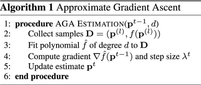
First of all, the method collects samples $(\mathbf {p}^{(l)}, f(\mathbf {p} ^ {(l)}))$, and stores them in a set $\mathbf {D}$ (Line 2). The method for collection could be, for example, using a uniform grid over the parameter space that includes the boundary points. After collecting a set of samples, the algorithm, in Line 3, fits a polynomial $\hat{f}$ of some specified degree d according to the collected samples. By fitting $\hat{f}$, the gradient $\nabla \hat{f}$ with some suitably chosen step size $\lambda ^t$ is calculated in the next Line 4. At the end, in Line 5, the estimated parameter is updated as presented in Equation 2.

$$\begin{aligned} \mathbf {p}^t = \mathbf {p}^{t-1} + \lambda ^t \nabla \hat{f}(\mathbf {p}^{t-1}) \end{aligned}$$

(2)

These steps define the AGA algorithm to estimate the agent’s parameters and type iteratively. For further details, we recommend reading Albrecht and Stone [2].

ABU In this method, rather than using $\hat{f}$ to perform gradient-based updates, Albrecht and Stone use $\hat{f}$ to perform Bayesian updates that retain information from past updates. Hence, in addition to the belief $\mathsf {P}(\theta _i |H^t_\omega )$, agent $\phi$ now also has a belief $\mathsf {P}(\mathbf {p}|H^t_\omega , \theta _i )$ to quantify the relative likelihood of parameter values $\mathbf {p}$, for agent $\omega$, when considering type $\theta _i$. This new belief is represented as a polynomial of the same degree d as $\hat{f}$. Algorithm 2 provides a summary of the Approximate Bayesian Update method.

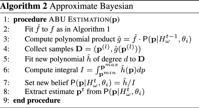
After fitting $\hat{f}$ (Line 2), the polynomial convolution of $\mathsf {P}(\mathbf {p}|H_\omega ^{t-1} , \theta _i )$ and $\hat{f}$ results in a polynomial $\hat{g}$ of degree greater than d (Line 3). Afterwards, in Line 4, a set of sample points is collected from the convolution $\hat{g}$ in the same way that is done in Approximate Gradient Ascent, and a new polynomial $\hat{h}$ of degree d is fitted to the collected set in Line 5. Finally, the integral of $\hat{h}$ under the parameter space, and the division of $\hat{h}$ by the integral is calculated, to obtain the new belief $\mathsf {P} (\mathbf {p}|H_\omega ^t, \theta _i )$. This new belief can then be used to obtain a parameter estimation, e.g., by finding the maximum of the polynomial or by sampling from the polynomial. For further details, we recommend reading Albrecht and Stone’s work [2].

POMCP Although in the MDP model agent $\phi$ has full observation of the environment, it cannot observe the type and parameters of its teammates. Therefore, we can employ POMCP [37], a state-of-the-art on-line planning algorithm for POMDPs (Partially Observable Markov Decision Process) [25]. POMCP stores a particle filter at each node of a Monte Carlo Search Tree. In this case, like the environment, apart from the types and parameters of the other agents, is fully observable, the particles are defined as different combinations of the types and parameters for all agents in $\varvec{\Omega }$. I.e., [($\theta _4, \mathbf {p}_1$), ($\theta _2, \mathbf {p}_2$), ..., ($\theta _1, \mathbf {p}_n$)], where each ($\theta , \mathbf {p}$) corresponds to one non-learning agent.

In the very first root, when the particles are created, we randomly assign types and parameters for each agent at each particle. Therefore, at every iteration, we sample a particle from the particle filter of the root, and hence change the estimated type and parameters of the agents. As in the POMCP algorithm, the root gets updated once a real action is taken, and a real observation is received. Therefore, for having a type probability $\mathsf {P}(\theta )_\omega$ for a certain agent $\omega$, we calculate the frequency that the type $\theta$ is asssigned to $\omega$ in the current root’s particle filter. Additionally, for the parameter estimation, we will consider the average across the particle filter (for each type and agent combination). For further explanations about the POMCP algorithm, we recommend reading Silver and Venesss [37].

6 On-line estimators for ad-hoc task execution

In this section, we introduce our novel algorithm, On-line Estimators for Ad-hoc Task Execution (OEATE), which helps the ad-hoc agent $\phi$ to learn the parameters and types of non-learning teammates autonomously. The main idea of the algorithm is to observe each non-learning agent ($\omega \in \varvec{\Omega }$) and record all tasks ($\tau \in \mathbf {T}$) that any one of the agents accomplishes, in order to compare them with the predictions of sets of estimators. In OEATE, there are some fundamental concepts applied during the process of estimating parameters and types. Therefore, we introduce the concepts first and, then, explain the algorithm in detail.

6.1 OEATE fundamentals

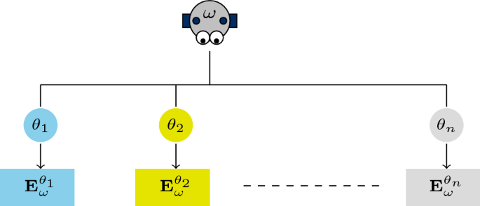
Sets of Estimators In OEATE, there are sets of estimators $\mathbf {E}^{\theta }_{\omega }$ for each type $\theta$ and each agent $\omega$ that the agent $\phi$ reasons about (Fig. 1). Moreover, each set $\mathbf {E}^{\theta }_{\omega }$ has a fixed number of N estimators $e \in \mathbf {E}^{\theta }_{\omega }$. Therefore, the total number of sets of estimators for all agents are $|\varvec{\Omega }| \times |\varvec{\Theta }|$. Figure 1 presents this idea, relating agent, types and estimators.

Fig. 1

For each $\omega$ agent there is a set of estimators $\mathbf {E}^{\theta }_{\omega }$ for each type

An estimator e of $\mathbf {E}^{\theta }_{\omega }$ is a tuple: $\{\mathbf {p}_e, {c}_e, {f}_e, {\tau }_e\}$, where:

• $\mathbf {p}_e$ is the vector of estimated parameters for $\omega$, and each element of the parameter vector is defined in the corresponding element range.

• ${c}_e$ holds the success score of each estimator e in predicting tasks.

• ${f}_e$ holds the failures score of each estimator e in predicting tasks.

• $\varvec{\tau }_e$ is the task that $\omega$ would try to complete, assuming type $\theta$ and parameters $\mathbf {p}_e$. By having estimated parameters $\mathbf {p}_e$ and type $\theta$, we assume it is easy to predict $\omega$’s target task at any state.

The success and failure scores ($c_e$ and $f_e$, respectively) will be further explained the in the Evaluation step of OEATE  presentation.

All estimators are initialised in the beginning of the process and evaluated whenever a task is done (by the $\omega$ agent alone or cooperatively). The estimators that are not being able to make good predictions after some trials are removed and replaced by estimators that are created using successful ones, or purely random, in a fashion inspired by GA [24].

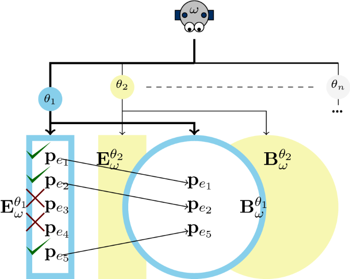
Bags of successful parameters Given the vector of parameters $\mathbf {p}_e = <p_1, p_2, \ldots , p_n>$, if any estimator e succeeds in task prediction, we keep each element of the parameter vector $\mathbf {p}_e$ in bags of successful parameters to use them in the future during new parameter vector creation. Accordingly, there is a bag of parameters $\mathbf {B}_\omega ^{\theta }$ for each type $\theta \in \varvec{\Theta }$ as there is a estimator set $\mathbf {E}^{\theta }_\omega$ for each type. These bags are not erased between iterations, hence, their size may increase at each iteration. There is no limit size for the bags. We will provide more details in Sect. 6.2. Figure 2 presents this idea, relating agent, types and estimators to the addition of estimators in the bags.

Fig. 2

For each $\omega$ agent and each possible type $\theta \in \Theta$, there is a bag of successful estimators. Successful estimator are copied to the bag of estimators of their respective type, in order to later generate new combinations of their elements. The check mark indicates success in predicting the task and the cross mark indicates failure

Choose Target State In the presented task-based ad-hoc teamwork context, besides estimation of type and parameter for each non-learning agent ($\omega \in \varvec{\Omega }$), the learning agent $\phi$ must be able to estimate the Choose Target State ($\mathfrak {s}_e$) of each $\omega$. The Choose Target State of an $\omega$ agent can be any $s \in S$ or, in other words, a non-learning agent $\omega$ can choose a new task $\tau \in T$ to pursue at any time t or state s. This can happen in many situations, for example, when the agent $\omega$ notices that its target is not existing anymore (if it was completed by other agents), it would choose a new target, and the Choose Target State would not be the same state as when the last task was done by agent $\omega$. Hence, a task-based estimation algorithm must be able to identify these moments where a possible task decision happened, to correctly predict the target.

Example For a better understanding of our method’s fundamentals, we will present a simple example. Let us consider a foraging domain [2, 41], in which there is a set of agents in a grid-world environment as well as some items. Agents in this domain are supposed to collect items located in the environment.

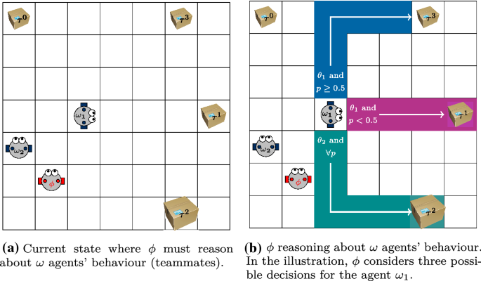
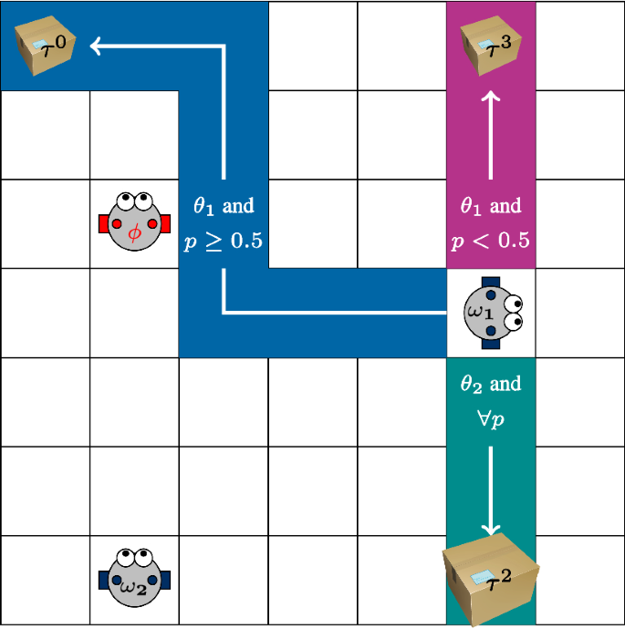
We show a simple scenario in Fig. 3, in which there are two non-learning agents $\omega _1$, $\omega _2$, one learning agent $\phi$, and four items which are in two sizes. As in all foraging problems, each task is defined as collecting a particular item, so in this scenario there are four tasks $\tau ^i$. In addition, we have two types $\theta _1$ and $\theta _2$, and two parameters ($p_1, p_2$), where $p_1, p_2 \in [0, 1]$.

Fig. 3

Example of $\phi$ thinking about $\omega$ agents’ behaviour, when performing foraging

To keep the example simple, we consider that only $p_1$ affects $\omega _1$’s decision-making at each state, and its behaviour follows the rules:

• If the type is $\theta _1$, and $p_1 \ge 0.5$, then $\omega _1$ goes towards small and furthest item ($\tau ^3$).

• If the type is $\theta _1$, and $p_1 < 0.5$, then $\omega _1$ goes towards small and closest item ($\tau ^1$).

• If the type is $\theta _2$, $\forall p_1 \in [0, 1]$, $\omega _1$ goes towards big and closest item ($\tau ^2$).

Therefore, in the example scenario, there are four sets of estimators, two for each $\omega$ agent : $\mathbf {E}^{\theta _1} _{\omega _1}$, $\mathbf {E}^{\theta _2}_{\omega _1}$, $\mathbf {E}^{\theta _1} _{\omega _2}$, $\mathbf {E}^{\theta _2}_{\omega _2}$. We assume that the total number of estimators in each set is 5 ($N=5$). Furthermore, we maintain 4 bags of estimators : $\mathbf {B_{\omega _1}^{\theta _1}}$, $\mathbf {B}^{\theta _2}_{\omega _1}$, $\mathbf {B}^{\theta _1} _{\omega _2}$, $\mathbf {B}^{\theta _2}_{\omega _2}$.

We assume that the true type of agent $\omega _1$ is $\theta _1$, and the true parameter vector is (0.2, 0.5). At this point, we will focus on the set of estimators for agent $\omega _1$. Moreover, we will continue to use this example to explain further details of OEATE  implementation.

6.2 Process of estimation

After presenting the fundamental elements of OEATE, we will explain how we define the process of estimating the parameters and type for each non-learning agent. Simultaneously, we will also demonstrate how OEATE  evolves in various steps, using our above example. The algorithm is divided into five steps, which is executed for all agents in $\varvec{\Omega }$ at every iteration:

• (i) Initialisation: responsible for initialising the estimator set and the bags of successful estimators for each agent $\omega \in \varvec{\Omega }$.

• (ii) Evaluation: step where OEATE  will increase the failure or the success score of each estimator, for all initialised estimator sets, based on the correct prediction of the $\omega$’s target task. If the estimator successfully predicts the task, it will be added to its respective bag. Otherwise, it will be up for elimination.

• (iii) Generation: step where our method replaces the estimators removed in the evaluation process for new ones.

• (iv) Estimation: process of calculating the types’ probabilities and expected parameters’ value for each existing estimators set. The calculation is based on the success rate of each set.

• (v) Update: responsible for analysing the integrity of each estimator e and its respective chosen target $\tau _e$ given the current world state. If it finds some inconsistency, a new prediction is made considering $\omega$’s perspective.

These steps are explained in detail below:

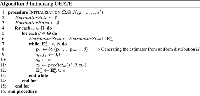
Initialisation At the very first step, for each identified teammate in the environment, we initialise its estimation set and the bag for each possible type. Therefore, agent $\phi$ needs to create N estimators for each type $\theta \in \varvec{\Theta }$ and each $\omega \in \varvec{\Omega }$. If there is a lack of prior information, the parameter vectors $\mathbf {p}_e$ of each estimator can be initialised with a random value from the uniform distribution $\mathcal {U}$, in each parameter’s range. Since each estimator has a certain type $\theta$ and a certain parameter vector $\mathbf {p}_e$, it allows agent $\phi$ to estimate agent $\omega$’s task choosing process. A task will be estimated and assigned to $\tau _e$ when, in a given state $s \in S$ at the time t, the prediction return a valid task. In the case where there is no valid task to return at the state s and time t, $\tau _e$ receives “None” and will be updated in later iterations (process carried out by the Update step). Finally, both ${c}_e$ and ${f}_e$ are initialised to zero.

The Algorithm 3 presents the initialisation process.

Initialisation Example Returning back to our example, in Initialisation step, we start by creating random estimators, as shown in Table 1. To make the example simple, we define the state as only the position of agent $\omega _1$. Therefore, we set each $\mathfrak {s}_e$ (Choose Target State) with the initial position of $\omega _1$, which is (3, 4), and then we create the parameter vectors $\mathbf {p}_e$ by randomly sampling from the uniform distribution, which should be done separately for both $p_1$ and $p_2$. Agent $\phi$ simulates $\omega _1$’s task decision-making process for each estimator in the sets $\mathbf {E}^{\theta _1}_{\omega _1}$ and $\mathbf {E}^{\theta _2}_{\omega _1}$, and obtains the corresponding target task $\tau _e$ based on the type and parameter of each estimator. In addition, all $f_e$ and $c_e$ will be initialised as zero. All initial estimators for both sets are shown in Table 1.

Table 1 Estimator sets $\mathbf {E}^{\theta _1} _{\omega _1}$ and $\mathbf {E}^{\theta _2}_{\omega _1}$ obtained from the Initialisation step

Evaluation The evaluation of all sets of estimators $\mathbf {E}^{\theta }_\omega$ for a certain agent $\omega$ starts when it completes a task $\tau _\omega$. The objective of this step is to find the estimators that could estimate $\omega$’s just completed real task $\tau _\omega$ correctly. Therefore, we present the Algorithm 4 to facilitate the understanding and explanation of the evaluation process.

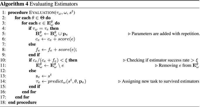
As there are sets of estimators for each type $\theta \in {\varvec{\Theta }}$, then for every e in $\mathbf {E}^{\theta }_\omega$, we check if the $\tau _{e}$ (estimated task by assuming $\mathbf {p}_e$ to be $\omega$’s parameters with type $\theta$) is equal to $\tau _{\omega }$ (the real completed task). If they are equal, we consider them as successful parameters and save the $\mathbf {p}_e$ vector in the respective bag $\mathbf {B}_\omega ^{\theta }$ (Line 5). The union between bag and parameter, which is applied in the equation, means that new parameters would be added to the bag with repetition, and if a parameter succeeds many times, it will appear in the bag with the same numbers of successes, so the chance of selecting it would be higher.

If the estimated task $\tau _e$ is equal to the real task $\tau _{\omega }$, we will increase the $c_e$ following $c_e \leftarrow c_e + score(e)$. The score(e) value denotes the information-level score for the prediction made by estimator e. The information-level score is used to represent the weighting given to certain task completions over others. For example: If a task prediction occurs many steps before the task completion, it was likely made by a correct estimator than by random chance. Furthermore, this function can be tweaked in a domain-specific way.

If the estimated task $\tau _e$ is not equal to the real task $\tau _{\omega }$, we will increase the $f_e$ score following $f_e \leftarrow f_e + score(e)$. Note from the algorithm that we will only remove an estimator e if its success rate is lower than $\xi$ (Line 10). We define the threshold $\xi$ as a success threshold aiming to improve our estimator set, by removing the estimators that do not make good predictions and keeping the ones that do (more detail in the Generation explanation).

Note that, by using this approach, any generated estimator e has a chance to be eliminated at the first iteration of estimation. Hence, some estimators, which may potentially approximate well the actual parameters, can be removed after performing their first estimation wrongly, $\forall \xi \in [0,1]$. However, even if these particles fail at the beginning of the estimation, other estimators may also likely fail in the subsequent iterations of OEATE, enabling the regeneration of the removed potentially correct estimator through the bags or by sampling it again from the uniform distribution. As we will show in Section 6.3, OEATE estimates the correct parameter for all agents as the number of completed tasks grows and under some assumptions.

Finally, the Choose target State ($\mathfrak {s}_e$) of the successful estimators is updated and a new task ($\tau _{e}$) is predicted using the type and parameters of the estimator. The evaluation process ends and the removed estimators will be replaced by new ones in the Generation Process.

Evaluation Example From the previous example, after the initialisation, the agents move towards their respective targets. Based on the true type and parameters of the agent $\omega _1$, after some iterations, the agent ($\omega _1$) gets the item that corresponds to the task $\tau ^1$. For this example, and throughout our experimentation, we will use the number of steps required between predicting the task and completing the next task as the score (information-level) for the estimator for that prediction. Let us assume that the number of steps required by the agent $\omega _1$ is 4 (3 for moving and 1 for completing). From Fig. 4, the agent $\omega _1$’s new position will be (6,4). We will use this value as the score for the estimators. Note that here, since all estimators chose the task at the same time, they will get the same score.

Whenever a task is done by an agent, the process of evaluation will start. Now, we carry out the next step of our process. In Evaluation, all estimators of the two sets $\mathbf {E}^{\theta _1} _{\omega _1}$, $\mathbf {E}^{\theta _2}_{\omega _1}$ will be evaluated. If the task $\tau$ of any estimator e equals to $\tau ^1$, then its success counter $c_e$ increases by score(e), otherwise it remains the same. Also, in failing cases, the counter of failures $f_e$ increases by score(e). The updated values of the estimators are shown in Table 2.

If we suppose that the threshold for removing estimators is equal to 0.5 ($\xi = 0.5$), then we will have two surviving estimators ($\frac{c_e}{c_e+f_e} \ge \xi$) at $\mathbf {E}^{\theta _1}_{\omega _1}$ and none in $\mathbf {E}^{\theta _2}_{\omega _1}$. Hence, the bag for $\theta _1$ are: $\mathbf {B}_{\omega _1}^{ {\theta _1}} = \{(0.4,0.6) , (0.2,0.5)\}$ and the bag for $\theta _2$ is empty. Further, the new Choose Target State will be (6,4) and using this, we can find the new task ($\tau _e$) for each of the surviving estimators. The new estimator sets are represented in Table 3 and, the new choose target state is illustrated by Fig. 4.

Table 2 Estimator sets $\mathbf {E}^{\theta _1} _{\omega _1}$, $\mathbf {E}^{\theta _2}_{\omega _1}$ after updating $c_e$ and $f_e$

Table 3 Estimator sets $\mathbf {E}^{\theta _1} _{\omega _1}$, $\mathbf {E}^{\theta _2}_{\omega _1}$ after Evaluation step

Fig. 4

New Choose Target state after $\omega _1$ completing $\tau ^1$. At this step, $\omega _1$ will try to find a new task to pursue

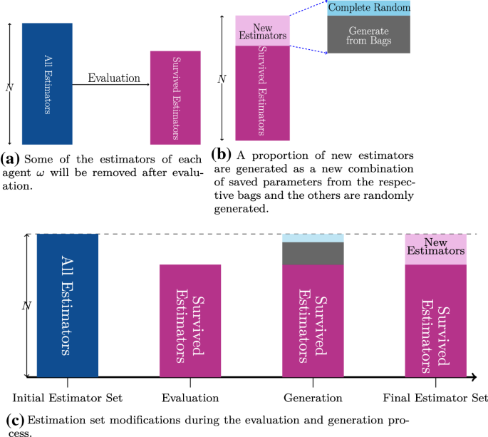
Generation The generation process of new estimators occurs after every evaluation process and only over the removed estimators. In this step, the objective is to generate new estimators, in order to maintain the size of the $\mathbf {E}^{\theta }_\omega$ sets equal to N.

Unlike the Initialisation step, we do not only create random parameters for new estimators, but generate a proportion of them using previously successful parameters from the bags $\mathbf {B}_\omega ^{\theta }$. Therefore, we will be able to use a new combination of parameters from estimators that had successful predictions at least one time in previous steps. Moreover, as the number of copies of the parameter $\mathbf {p}$ in the bag $\mathbf {B}_\omega ^{\theta }$ is equivalent to the number of successes of the same parameter in previous steps, the chance of sampling very successful parameters will increase according to its success rate.

The idea of using successful estimators to generate part of the new estimators is related to the Genetic Algorithm (GA) principles. Until now, the described process shares several similarities with the GA idea, such as the generation of a sample population for further evaluation and feature improvement. Furthermore, we are concerned about boosting our estimation process (based on the estimator sampling and evaluation), so we require a reasonable way to generate new estimators that can improve our estimation quality. Therefore, inspired by GAs mutation and cross-over process, we implement a GA-inspired process that supports our generation method.

Therefore, after the elimination of estimators for which the probability of making a correct prediction is lower than the threshold $\xi$, we will generate new estimators for our population following the mutation rate of m, where part of our population is generated randomly following a uniform distribution $\mathcal {U}$, and the rest following a process inspired by the cross-over, using our bags of successful parameters. With domain knowledge, different distributions could be used. Figure 5 illustrates how the estimator set changes during this described process and indicates the portion of particles generated using the bags or randomly. Algorithm 5 summarises this generation procedure.

Fig. 5

Estimation set modifications from the evaluation to the end of generation process. a, b present the modifications after the evaluation and after the generation, respectively. c Presents the entire modification process

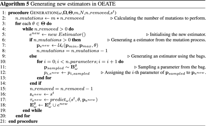
The generation process using the bags can be seen in Algorithm 5 Line 10-13 . There, a new estimator is created by sampling n different parameters (with repetition) from the target bag, and then choosing their $i\text {-th}$ parameters. Hence, essentially if the parameter of new estimator ($e^{new}$) is $\mathbf {p}_{e^{new}} = <p_1, p_2, \ldots , p_n>$, then $p_i$ is chosen by sampling $\mathbf {p}_{sampled} \sim \mathbf {B}_{\omega }^{\theta }$ and then taking the i-th parameter from it ($p_{i,{sampled}}$).

After performing all the generations with the bag, we continue to fill the estimator set with uniform generated parameters. Once the estimator set is full (i.e., $|\mathbf {E}_{\omega }^{\theta }| = N$), the current state is assigned as Choose Target State ($\mathfrak {s}_{e^{new}}$) of every new estimator. Afterwards, a task ($\tau _{e^{new}}$) is predicted for each new estimator and the generation process finishes.

Generation Example Supposing $m = \frac{1}{3}$ as mutation rate, then $(1 - \frac{1}{3}) \times (5-2) = 2$ new estimators are generated by randomly sampling from the bags, while $\frac{1}{3} \times (5-2) = 1$ estimator is generated randomly from the uniform distribution. Therefore, we may create new estimators with the following parameters: (0.4, 0.5); (0.2, 0.6); (0.8, 0.7), where the last vector is fully random. For $\mathbf {E}^{\theta _2}_{\omega _1}$, as all estimators were removed and the corresponding bags are empty, the whole set $\mathbf {E}^{\theta _2}_{\omega _1}$ will be generated using the uniform distribution as in the initialisation process. After this, the current state (6,4) , is assigned as the Choose Target State for each new estimator and a task is predicted. All new estimators and updated values are shown in Table 4.

Table 4 Estimator sets $\mathbf {E}^{\theta _1} _{\omega _1}$ and $\mathbf {E}^{\theta _2}_{\omega _1}$ sets after the Generation step

Estimation At each iteration after doing evaluation and generation, it is required to estimate a parameter and type for each $\omega \in \varvec{\Omega }$ to improve the decision-making. First, based on the current sets of estimators, we calculate the probability distribution over the possible types. For calculating the probability of agent $\omega$ having type $\theta$, $\mathsf {P}(\theta )_\omega$, we use the success score $c_e$ of all estimators of the corresponding type $\theta$. For each $\omega \in \varvec{\Omega }$, we add up the success rates $c_e$ of all estimators in $\mathbf {E}^\theta _\omega$ of each type $\theta$, that is:

$$\begin{aligned} k^\theta _\omega = \sum _{e \in \mathbf {E}^\theta _\omega } c_e,~ \forall \theta \in \varvec{\Theta } \end{aligned}$$

It means that we want to find out which set of estimators is the most successful in estimating correctly the tasks that the corresponding non-learning agent completed. In the next step we normalise the calculated $k^\theta _\omega$, to convert it to a probability estimation, following:

$$\begin{aligned} \mathsf {P}(\theta )_\omega = {\left\{ \begin{array}{ll} \frac{k^\theta _\omega }{\sum _{\theta ' \in \varvec{\Theta }} k^{\theta '}_\omega } &{} {\sum _{\theta ' \in \varvec{\Theta }} k^{\theta '}_\omega } > 0 \\ \frac{1}{N} &{} \text {else} \end{array}\right. } \end{aligned}$$

During the simulations, OEATE  will sample estimations from the current estimation sets. In detail, for each agent $\omega$, we will sample a type $\theta$ based on $P(\theta )_\omega$ and sample an estimator from $\omega$’s estimator set of that type ($\mathbf {E}_\omega ^\theta$), using the weights given by $c_e$ of the estimators. In this way, once a type ($\theta$) is selected, the probability of selection of each estimator $e \in \mathbf {E}_\omega ^{\theta }$ is equals to $c_e/k_\omega ^\theta$ . If $k_\omega ^{\theta } = 0$, we sample the estimator uniformly from $\mathbf {E}_{\omega }^{\theta }$. Otherwise, we perform the weighted sampling.

Using this strategy, OEATE  can improve the reasoning horizon and diversify the simulations. Differently from AGA and ABU that presents only a single estimation per iteration, we present a set of the (current) best found estimators for planning and decision-making.

Estimation Example Now, we do the Estimation step in our example to have a probability distribution over types, and one parameter vector per type of $\omega _1$. At this step, in order to find the probability of being either $\theta _1$ or $\theta _2$, we apply the Equation 6.2. By considering the $c_e$ of all estimators, we have that:

$$\begin{aligned} k^{\theta _1} = 8, k^{\theta _2} = 0, \end{aligned}$$

Hence, to calculate the probability of each type, we use the Equation 6.2. Accordingly, the probabilities are:

$$\begin{aligned} \mathsf {P}'(\theta _1) =\frac{8}{8 + 0}=1, \mathsf {P}'(\theta _2) = \frac{0}{8 + 0}=0, \end{aligned}$$

which means that the probability of being $\theta _1$ is the higher one.

Now, for the sampling process, we sample a type using the previously calculated distribution. Let’s say that we sample $\theta _1$. Now, from this type, we also sample an estimator, using the ratio $c_e/k^{\theta _1}$ as the probability of each estimator in $E_{\omega _1}^{\theta _1}$. Concretely, we get:

$$\begin{aligned} \mathsf {P}((0.4,0.6)| \theta _1) = \frac{4}{8} , \mathsf {P}((0.2,0.5)| \theta _1) = \frac{4}{8} \end{aligned}$$

while the other estimators have probability 0. So, we use these probabilities to sample an estimator, let’s say (0.4,0.6). Therefore, type $\theta _1$ and the parameters (0.4, 0.6) will be our estimated type and parameter for the current estimation step.

During the planning phase in the root of the MCTS (for the learning agent $\phi$ perspective), the OEATE  will sample the simulating type and parameter respecting the probabilities calculated above. Moreover, to calculate the error of the estimation of our method, we use the mean square error (MSE) between the true parameter and the expected parameter of the true type ($\theta ^*$). The expected parameter of a type ($\theta$) and agent $\omega$ is calculated as:

$$\begin{aligned} \mathbf {p}_{exp} = \sum _{e \in \mathbf {E}_{\omega } ^{\theta }} \frac{c_e}{k_{\omega }^{\theta }} \mathbf {p}_e \end{aligned}$$

Update As mentioned earlier, there are possible issues that might arise in our estimation process, they occur:

(i):

when a certain task $\tau$ is accomplished by any of the team members (including agent $\phi$), and some other non-learning agent was targeting to achieve it, or;

(ii):

when a certain non-learning agent is not able to choose a task to target (e.g., cannot see or find any available (or valid) task within its vision area considering possible parameters limitations, such as vision radius and angle).

If some non-learning agent $\omega$ faces one of these problems, it will keep trying to find a task to pursue. Hence, from the perspective of the learning agent $\phi$, OEATE must handle this problem updating its teammates’ targets. Otherwise, it might incorrect evaluate the available estimators given the outdated prediction.

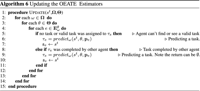
Therefore, the OEATE’s Update process exists to guarantee the estimator set integrity for future evaluation. At each iteration, the update step will analyse the integrity of each estimator e and its respective chosen target $\tau _e$ given the current world state. If it finds some inconsistency, it will simulate the estimator’s task selection for the next states, considering $\omega$’s perspective. The process is carried out in each successive state until it returns a new valid target for the indecisive estimator. The Algorithm 6 presents the described update routine.

Update Example In the update step, we look at our estimators from Table 4 and check whether the conditions for update (from Algorithm 6 ) are met. Evidently, for our case,we see that every estimator has a valid task assigned to it and therefore, nothing will happen in the update step.

6.3 Analysis

We show that as the number of tasks goes to infinite, under full observability, OEATE  perfectly identifies the type and parameters of all agents $\omega$, given some assumptions. Since each of our updates are related to completing the tasks, this analysis assumes that the agents are able to finish the tasks. First, we consider that parameters have a finite number of decimal places. This is a light assumption, as any real number x can be closely approximated by a number $x'$ with finite precision, without much impact in a real application (e.g., any computer has a finite precision). Hence, as each element $p_i$ in the parameter vector is in a fixed range, there is a finite number of possible values for it. To simplify the exposition, we consider $\psi$ possible values per element (in general they can have different sizes). Let n be the dimension of the parameter space.

Additionally, let $\mathbf {p^*}$ be the correct parameter, and $\theta ^*$ be the correct type, of a certain agent $\omega$. We define $\theta ^{-} \not = \theta ^*$, and $\mathbf {p}^{-} \not = \mathbf {p^*}$, representing wrong types and parameters, respectively. We will also use tuples $(\mathbf {p}, \theta )$ to represent a pair of parameter and type.

Assumption 1 Any $(\mathbf {p}, \theta ^{-})$, and any $(\mathbf {p}^{-}, \theta ^*)$ has a lower probability of making a correct task estimation than $(\mathbf {p^*}, \theta ^*)$. Moreover, we assume that the correct parameter-type pair $(\mathbf {p}^*,\theta ^*)$ will also be able to have the correct Choose Target State ($\mathfrak {s}_e$).

This assumption is very light because if a certain pair $(\mathbf {p}, \theta ^{-})$ or $(\mathbf {p}^{-}, \theta ^*)$ has a higher probability of making correct task predictions, then it should indeed be the one used for planning, and could be considered as the correct parameter and type pair.

Assumption 2 Any $(\mathbf {p}, \theta ^{-})$, and any $(\mathbf {p}^{-}, \theta ^*)$ will not succeed infinitely often. That is, as $|\mathbf {T}| \rightarrow \infty$ there will be cases where it successfully predicts the task, but the number of cases is limited by a finite constant c.

Assumption 3 This assumption is needed to distinguish our method from a random search. The assumption has 2 parts: (i) a correct value $p_i^*$ in any position i may still predict the task wrongly (since other vector positions may be wrong), but it will eventually predict at least one task correctly in at most t trials, where t is a constant; (ii) a wrong value $p_i^{-}$ in any position i may still predict the task correctly (since other vector positions may be correct), but that would happen at most $\mathfrak {b}$ times for each bag, across all wrong values. Therefore, $\mathfrak {b} \ll \psi$.

That is, if one of the vector positions i is correct, $\mathbf {p}$ will not fail infinitely, even though other elements may be incorrect. That is valid in many applications, as in some cases only one element is enough to make a correct prediction. For example, if a task was nearby, for almost any vision radius it would be predicted as the next one if the vision angle were correct. On the other hand, wrong values will not always succeed. That is also true in many applications: although by the argument above, wrong values may make correct predictions, but these are a limited number of cases in the real world. Eventually, all tasks nearby will be completed, and a correct vision radius estimation becomes more important to make correct predictions. Usually, $\psi$ would be large (e.g., they may approximate real numbers), so we would have $\mathfrak {b} \ll \psi$. Additionally, we will consider the case with lack of previous knowledge, so parameters and types will be initially sampled from the uniform distribution. As before, we denote by $\mathsf {P}(\theta )$ the estimated probability of a certain agent having type $\theta$, but we drop the subscript $\omega$ for clarity.

Theorem 1

OEATE  estimates the correct parameter for all agents as $|\mathbf {T}| \rightarrow \infty$. Hence, $\mathsf {P}(\theta ^{*}) \rightarrow 1$.

Proof

Since wrong parameters-type pairs will not succeed infinitely often, we always will generate new estimators with a random $\mathbf {p}_e$. As we sample from the uniform distribution, $\mathbf {p}^*$ will be sampled with probability $1/\psi ^n > 0$. Hence, eventually it will be generated as $|\mathbf {T}| \rightarrow \infty$. As the generation defines a Bernoulli experiment, from the geometric distribution, we expect $\psi ^n$ trials.

Therefore, eventually, there will be an estimator with the correct parameter vector $\mathbf {p^*}$. Furthermore, since $(\mathbf {p^*}, \theta ^*)$ has the highest probability of making correct predictions (Assumption 1), it has the lowest probability of reaching the failure threshold $\xi$. Hence, as $|\mathbf {T}| \rightarrow \infty$, there will be more estimators $(\mathbf {p^*}, \theta ^*)$, than any other estimator. Further, any $(\mathbf {p^{-}}, \theta ^*)$ will eventually reach the failure threshold, and will eventually be discarded, since it succeeds at most c times by Assumption 2. Therefore, by considering our method of sampling an estimator from the estimator sets, we will correctly estimate $\mathbf {p^*}$ when assuming type $\theta ^*$. Hence, when $|\mathbf {T}| \rightarrow \infty$ the sampled estimator from $\mathbf {E}^{\theta ^*}_\omega$ will be $\mathbf {p^*}$.

Further, when we consider the Assumption 2 , then the probability of the correct type $\mathsf {P}(\theta ^*) \rightarrow 1$. That is, we have that $c_e \rightarrow \infty$ in the set $\mathbf {E}^{\theta ^*}_\omega$. Hence, $k^{\theta ^*}_\omega \rightarrow \infty$, while $c_e < c$ for $\theta ^{-}$ (by assumption). Therefore:

$$\begin{aligned} \mathsf {P}(\theta ^*) = \frac{k^{\theta ^*}_\omega }{\sum _{\theta ' \in \varvec{\Theta }} k^{\theta '}_\omega } \rightarrow 1, \end{aligned}$$

while $\mathsf {P}(\theta ^{-}) \rightarrow 0$, as $|\mathbf {T}| \rightarrow \infty$. $\square$

This ensures that the as $|\mathbf {T}| \rightarrow \infty$, the sampled type is $\theta ^*$.

We saw in Theorem 1 that a random search from the mutation proportion takes $\psi ^n$ trials in expectation. OEATE , however, finds $\mathbf {p}^*$ much quicker than that, since a proportion of estimators are sampled from the corresponding bags $\mathbf {B}_\omega ^{\theta , i}$. In the following proposition, we will prove that OEATE  will indeed find $\mathbf {p}^*$ and under Assumption 1, $\mathbf {p}^*$ would have highest probability of not being removed from the estimator set and will continue to add it’s own parameters back to the bag, thereby further increasing the probability of sampling those parameters at each mutation.

Proposition 1

OEATE  finds $\mathbf {p}^*$ in $O(n \times \psi \times (\mathfrak {b}+1)^n)$.

Proof

Consider Assumption 3, we know that at some time, we must encounter a parameter value $p_i$. Sampling the correct value for element $p_i$ would take $\psi$ trials in expectation. Once a correct value is sampled, it will be added to $\mathbf {B}_{\omega }^{\theta ^*}$ if it makes at least one correct task prediction. It may still make incorrect predictions because of wrong values in other elements, and it would be removed (from the estimator set) if it reaches the failure threshold $\xi$. However, for a constant number of trials $t \times \psi$, it would be added to $\mathbf {B}_{\omega }^{\theta ^*}$. Similarly, sampling the correct value for all n dimensions at least one time would take $n \times \psi$ trials in expectation, and in at most $t \times n \times \psi$ trials $\mathbf {B}_{\omega }^{\theta ^*}$ would have at least one estimator each with the correct value in position i. The bags store repeated values, but in the worst case, there is only one correct example at each $\mathbf {B}_{\omega }^{\theta ^{*}}$, leading to at least $1/(\mathfrak {b}+1)$ probability to sample the correct value from the bag. Hence, given the bag sampling operation, we would find $\mathbf {p}^*$ with at most $t \times n \times \psi \times (\mathfrak {b}+1)^n$ trials in expectation.

Hence, the complexity is close to $O(\psi )$, instead of $O(\psi ^n)$ as the random search (since $\mathfrak {b} \ll \psi$).

Considerations In Assumption 1, the choose target state $(\mathfrak {s}_e)$ of an estimator is dependent only on the previous predicted tasks and the main agent’s observation. Therefore, in a fully observable case, the true parameters have the highest probability of having the correct choose target state . Furthermore, we leave the proof for partially observable cases as future work.

Time Complexity It is worth noting that the actual time taken by the algorithm is dependent on $(\mathfrak {b}+1)^n$ . So, as an example, if $\mathfrak {b}=10 \ll \psi =100$ , then if $n=3$ , $(\mathfrak {b}+1)^n =1000 \gg \psi = 100$ . However, when we are write the time complexity, we are focusing on how the algorithm will scale with larger search space (i.e. Higher $\psi$). Further, since $\psi$ is the precision of parameters, it is likely to be a large value. For instance, if there are 3 elements in parameter vector ($\mathbf {p}$), if range of each element ($p_i$) is [0,1] and we want our answer to be accurate up to only 3 places of decimal, then $\psi = 10^3$ .

6.4 OEATE with partial observability

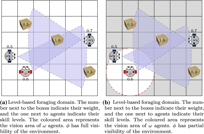
Assuming full visibility for the learning agent is a strong presupposition and it rarely occurs in a real application (due to data or technology limitations). Thus, towards a more realistic application, we considered scenarios where agent $\phi$ is working with limited visibility of the environment. Therefore, we formalise our problem as a Partially Observable Markov Decision Process, and similarly as before, we define a single agent POMDP model, which will allow us to adapt POMCP [37] with our On-line Estimators for Ad-hoc Task Execution.

In this section, we will outline the main changes compared to our previous MDP model (Sect. 2) and how we designed our POMCP-based solution for distributed task execution problems into an ad-hoc teamwork context.

6.4.1 POMDP model

Our POMDP model considers one agent $\phi$ acting in the same environment as a set of non-learning agents ($\omega \in \varvec{\Omega }$), and $\phi$ tries to maximise the team performance without any initial knowledge about $\omega$ agents’ types and parameters. We consider the same set of states $\mathcal {S}$, action $\mathcal {A}$, transition $\mathcal {T}$ and reward function $\mathcal {R}$ defined previously. Additionally, agent $\phi$’s objective is still to maximise the expected sum of discounted rewards. However, now agent $\phi$ has a set of observations $\mathcal {O}$ that defines its current state. Every action a produces an observation $o \in \mathcal {O}$, which is the visible environment in agent $\phi$’s point of view (all of the environment within the visibility region, in the state $s'$ reached after taking action a). We assume agent $\phi$ can perfectly observe the environment within the visibility region, but it cannot observe anything outside the visibility region. Hence, our POMDP model workswithin a observation function which is deterministic instead of stochastic—so, all values denote empty square, agent or task. As before, agents true types and parameters are not observable.

The current state cannot be observed directly by agent $\phi$, so it builds a history $\mathcal {H}$ instead. $\mathcal {H}$ consists of a set of collected information $h_t$ from the initial timestamp $t=0$ until the current time. Each $h_t$ is an action and observation pair ao, representing the action a taken at time t, and the corresponding observation o that was received. The current agent history will define its belief state, which is a probability distribution across all possible states. Therefore, agent $\phi$ must find the optimal action, for each belief state.

This formalisation enables the extension of our planning model, from a full observable context using MCTS to a partially observable context for POMCP application. This transition to a POMCP application is a straightforward process, however, we make further modifications to guarantee the on-line estimation and planning features, which OEATE  presents.

6.4.2 POMCP modification

POMCP [37] is an extension of UCT for problems with partial observability. The algorithm uses an unweighted particle filter to approximate the belief state at each node in the UCT tree and requires a simulator, which is able to sample a state $s'$, reward r and observation o, given a state and action pair. Each time we traverse the tree, a state is sampled from the particle filter of the root. Given an action a, the simulator samples the next state $s'$ and the observation o. The pair ao defines the next node n in the search tree, and for the current iteration, the state of the node will be assumed to be $s'$. This sampled state $s'$ is added to node n’s particle filter, and the process repeats recursively down the tree. We refer the reader to Silver and Veness [37] for a detailed explanation.

However, as in the UCT case, we do not know the true transition and reward functions, since they depend on the pdfs of the non-learning agents ($\omega \in \varvec{\Omega }$). Therefore, we employ the same strategy as previously: at each time we go through the search tree, we sample a type for each agent from the estimated type probabilities and use the parameters that correspond to the sampled type. These remain fixed for the whole traversal until we re-visit the root node for the next iteration. Note that these sampled types and parameters are also going to be used in the POMCP simulator, when we sample a next state, a reward and an observation after choosing an action in a certain node.

As mentioned previously, POMCP has been modified before to sample transition functions [20]. Here, however, we are employing a technique that is commonly used in UCT (for MDPs) in ad-hoc teamwork [2, 7], but now in a partially observable scenario, which allows us to work on the type/parameter space instead of directly on the complex transition function space. In this way, we can then employ OEATE  for the type and parameter estimation.

The same OEATE  algorithm described in Sect. 6 can handle the cases where any agent $\omega \in \varvec{\Omega }$ is outside the agent $\phi$’s visibility region. In order to do so, it samples a particle from the POMCP root, which corresponds to sampling a state from the belief state. That allows us to have complete (estimated) states when predicting tasks for $\omega$ agents. States that are considered more likely will be sampled with a higher probability for the OEATE algorithm following the POMCP belief state filtering probabilities. However, we assume in our implementation (and in all algorithms we compare against) that agent $\phi$ knows when an agent $\omega$ has completed a task $\tau$, even if it is outside our visibility region. That is, agent $\phi$ would know exactly which task was completed by a certain agent. That would require in a real application some global signal of task completion (e.g., boxes with radio transmitters).

7 Results

7.1 Level-based foraging domain

The level-based foraging domain is a common problem for evaluating ad-hoc teamwork [2, 4, 41]. In this domain, a set of agents collaborate to collect items displaced in a rectangular grid-world environment in a minimum amount of time (Fig. 6). In this foraging domain, items have a certain weight, and agents have a certain skill level, which defines how much weight they can carry. Hence, agents may need to collaborate to pick up a particularly heavy item. Further, we assume that tasks are spawning in the environment during the execution.

Differently from [2, 41], this approach enables a continuous level of information in the scenario, which $\phi$ must analyse and reason about to improve the team’s performance. The performance here will regard the number of completed tasks in the environment instead of the necessary time to complete all tasks. Concretely, we define the number of tasks that can be in the environment simultaneously. If some agent (or group of agents) accomplishes a task, we spawn a new one for each completion at that execution time. In this way, we manage to maintain a fixed number of tasks in the environment, hence the same problem level from the beginning to the end.

Finally, we defined this problem over full and partial observability, which Fig. 6 illustrates possible scenarios configuration.

Fig. 6

Possible problem scenarios in the defined level-based foraging domain

Agent’s Parameters Each agent has a visibility region and can only choose items as a target if they are in its visibility cone. Therefore, to know which items are in the visibility area of each agent, we need to have the View Angle and the maximum View Radius of the agents. Additionally, each agent has a Skill Level which defines its ability to collect items. Also, each item has a certain weight, so each agent can collect items that have a weight below their Skill Level or equal to it. Based on what we described above, each agent can be defined by three parameters:

• l, which specifies the Skill Level and $l \in [0.5,1]$;

• a, which is referring to View Angle. The actual angle of the visibility cone is given by the formula $a * 2 \pi$. Additionally, it is assumed that $a \in [0.5, 1]$;

• r, which is referring to the View Radius of the agent. The actual View Radius is given by $r \sqrt{w^2+h^2}$, where w and h are the width and height of the grid. Also, the range of the radius is $r \in [0.5, 1]$.

All of these parameters are applicable to all $\omega \in \varvec{\Omega }$. Agent $\phi$ has the parameter Skill Level when it has either full or partial observability, but the View Angle and View Radius parameters are only applicable when it has partial observability.

Agent’s Types Concerning types of non-learning agents, we took inspiration from Albrecht and Stone [2] type definitions in the foraging domain. They considered four possible types for the agents in $\varvec{\Omega }$: two “leader” types, which choose items in the environment to move towards, and two “follower” types, which attempt to go towards the same items as other agents, in order to help them load items. However, “follower” agents may also choose other agents as target, while in our work we handle agents that choose tasks as target. Therefore, we only consider “leader” agents in our work. Hence, based on agent $\omega$’s type and parameter values, a target item will be selected, and the agent’s internal state (memory) will be set to the position of that target. Afterwards, the agent will move towards the target using the $A^*$ algorithm [21]. Here is the detail for how the different types choose their targets:

• L1: if there are items visible, return the furthest item; else, return $\varnothing$.

• L2: if there are items visible, return the item with highest sum of coordinates; else, $\varnothing$.

• L3: if there are items visible, return the closest item; else, return $\varnothing$.

• L4: if there are items visible, return the item with lowest sum of coordinates; else, $\varnothing$.

• L5: if there are items visible, return the first item found (considering the orientation: west to east, north to south); else, $\varnothing$.

• L6: if there are items visible, return an random item; else $\varnothing$.

Actions Each agent has five possible actions in the grid: North, South, East, West, Load.

The first four actions will move the agent towards the selected direction if the destination cell is empty and it is inside the grid.

The fifth action, Load, helps the agent to load its target item. The only time that an agent can collect an item is when the item is next to the agent, and the agent is facing it. Also, for loading the item, the Skill Level of the agent should be equal to or higher than the items’ weight. If the agent does not have enough Skill Level to collect the item, then a group of agents can do the job if the sum of the Skill Levels of the agents that surround the target is greater than or equal the item’s weight. Therefore, the item can be “loaded” by a set of agents or just one agent. In the situation when the agent does not have enough ability to collect the target item, it will standstill in the same place when issuing the Load action. In the case of collecting an item, the team of agents receives a reward and it will be removed from the grid.

Foraging Process: First of all, we describe the process of foraging and choosing a target for agents $\omega$ in Algorithm 7 in order to facilitate the understanding and explanation.

In the very first step as agent $\omega$ has not chosen any target, the Mem, which holds the target item, is initialised to $\emptyset$. In Line 10, the VisibleItems routine is called, which gets the agent $\omega$’s parameters, View Angle and View Radius, and returns a set containing the visible items. In Line 11, the ChooseTarget routine gets the Skill Level and Type of the $\omega$ agent, and the list of visible items, returned from VisibleItems routine as input. The output of this routine is the target item that agent $\omega$ should go towards.

As it is shown in Line 17, there might be cases where agent $\omega$ is not able to find any target task. In these cases, all actions would get equal probabilities and consequently, it will perform actions uniformly randomly until it is able to choose a task.

We should mention that this is an algorithm template that we assume non-learning agents are following. We use the same template in our simulations, but in practice agents, $\omega$ could follow different algorithms. Hence, in the results section, we will also evaluate the case where the agents do not follow the same algorithm as in our template.

7.2 Capture the prey domain

Intending to evaluate the present range of applicability of our proposal over different domains, we further perform experiments in the Capture-the-Prey domain.

This domain is presented as a discrete, rectangular grid-world as in Sect. 7.1. It is a variant of the Pursuit Domain described in [9, 10]. There are several “preys” in the environment, which represents the objectives that the Ad-hoc Team must pursue, similar to the “tasks” from our Level-based Foraging environment. However, the preys are also non-learning agents, which are running a reactive algorithm and trying to escape from being captured—defining decentralised tasks, which are moving in the scenario. Each prey can also be identified by a numeric index given to it. The ad-hoc team is composed of non-learning agents $\omega \in \varvec{\Omega }$ and a learning agent $\phi$. They must surround the prey and capture it, which means to block the movement of the prey on all discrete four sides: North, South, East and West. It can be done only by agents, or with the support of walls and/or by other preys. Note that surrounding is mandatory, hence the agents must collaborate in the most efficient way in order to improve their performance. The tasks are re-spawning in this environment as well. Figure 7 illustrates the problem.

Fig. 7

Possible problem scenario in the defined capture the prey domain. The agent with red details is the learning agent $\phi$. The agents with blue details are the non-learning agents $\omega \in \Omega$. The grey agents are the prey (Color figure online)

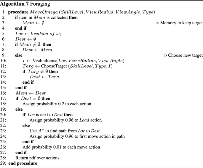
Agent’s Parameters The parameter of each agent is the same as earlier, but there is no longer a Skill Level parameter since the completion condition is not related to task parameters. In this way, the $\omega$ agents still have a visibility region to see and choose targets, which follows:

• a, which is referring to View Angle. The actual angle of the visibility cone is given by the formula $a * 2 \pi$. Additionally, it is assumed that $a \in [0.5, 1]$;

• r, which is referring to the View Radius of the agent. The actual View Radius is given by $r \sqrt{w^2+h^2}$, where w and h are the width and height of the grid. Also, the range of the radius is $r \in [0.5, 1]$.

Agent’s Types Concerning types of non-learning agents, we created 2 main types to run the experiments:

• C1: the spatial type of the set, which chooses the furthest visible prey to pursue, if there are visible preys in its vision area; else, return $\varnothing$.

• C2: the index-based type, which chooses preys with an even identification, if there are visible preys in its vision area; else, return $\varnothing$.

Actions Each agent has 5 actions : North, South, East, West, Block . The first four actions will move the agent towards the selected direction if the destination cell is empty or it is inside the grid. The Block is the action that actually captures the prey, where the agent stands at its position blocking the passage of prey. Notice that there is no Load action, as the completion of the task ( or “Capturing the Prey” ) is done by the surrounding. So the agent must block one passage of the prey, trying to create a capture situation.

Unlike in level-foraging, the tasks are no longer stationary. At each step, the tasks also move randomly to one of the empty squares next to them. If no such free space exists and, at least, one agent is surrounding the task, it gets captured. So, each task can be completed by at least 1 agent, depending on the location of the task and the whole state configuration (such as other agents positions, other preys positions and map borders).

Capturing Process Directly, the process of choosing actions and targets remains similar to the process defined for Foraging by Algorithm 7.

7.3 OEATE results

Baselines We will compare our novel algorithm (OEATE) against two state-of-the-art parameter estimation approaches in ad-hoc teamwork: AGA and ABU [2] (both presented in Sect. 5). As we mentioned before, we sample sets of parameters (for a gradient ascent step or a Bayesian estimation), which is similar to set of estimators in the OEATE  for estimating parameters and types. Therefore, for better comparison against them, we use the same set size as estimator sets (N). Note that Albrecht and Stone [2] also introduced an approach called Exact Global Optimisation (EGO). We do not include it in our experiments since it is significantly slower than the ABU/AGA, without outperforming them in terms of prediction.

Additionally, we compare our approach against the proposed POMCP-based method (also presented in Sect. 5) for type and parameter estimations. As described, in estimation with POMCP, we assume that the agent $\phi$ can see the whole environment, however, the teammates’ type and parameters are not observable. Hence, agent $\phi$ applies POMCP’s particle filter for estimation. We use $N \times |\varvec{\Omega }| \times |\varvec{\Theta }|$ particles, matching the total number of estimators in our approach (since we have N per agent, for each type).

Experiments configuration We executed random scenarios in Level-based Foraging and Capture the Prey domains (Sects. 7.1 and 7.2, respectively) for a different number of distributed tasks, agents and environment size for all aforementioned estimation methods. The experiment finishes by reaching 200 iterations. Every run was repeated 20 times, and we plot the average results and the confidence interval ($\rho = 0.05$). Therefore, when we say that a result is significant, we mean statistically significant considering $\varvec{\rho \le 0.05}$, according to the result of a Kruskal-Wallis test. In detail, as a first test, we applied the Kruskal-Wallis to determine whether a statistically significant difference exists between all the algorithms considered; afterwards, we evaluated each pair of algorithms using a Wilcoxon Rank Sum Test (with Bonferroni correction) to determine which ones were different from the others. Following these steps, we could accurately calculate the confidence interval in the results obtained by each approach, thus finding which one is significantly better than the others. We avoid presenting every p-value to improve the readability of the work. So, we maintain our focus on presenting the p-values that are meaningful for our analysis and avoid reporting the p-value for results where there is clearly no significance (i.e., $\varvec{\rho } \ge 0.05$). Note that error bars and coloured regions indicate the confidence interval at a $95\%$ confidence level, not the standard deviation, supporting the confidence visualisation.

For each scenario, we assume one of the four estimation methods ABU, AGA, POMCP and OEATE  to be agent $\phi$’s estimation method. We kept a history of estimated parameters and types for all iterations of each run and calculated the errors by having true parameters and true types in hand. Then, we evaluate the mean absolute error (as in Equation 6.2) for the parameters, and $1 -\mathsf {P}(\theta ^*)$ for type; and what we show in the plots is the average error across all parameters. Additionally, since we are aggregating several results, we calculate and plot the average error across all iterations.

In this way, we first fix the number of possible types as 2 (L1, L2 and C1, C2 for Level-based Foraging and Capture the Prey domains, respectively), and later we show the impact of increasing the number of types. Type and parameters of agents in $\varvec{\Omega }$ are chosen uniformly randomly. At the Level-based Foraging environment, the skill level for agent $\phi$ is also randomly selected. Every parameter $p_i \in \mathbf {p}$ is a value within the minimum-maximum interval $[p_i^{min}, p_i^{max}] = [0.5,1.0]$.

Every task is created in random positions, but we exclude the scenario’s borders and free the adjacent tiles. That allows agents to set up their positions to perform the load action from any direction (i.e., North, South, East, West), making it always possible for 4 to simultaneously load an item, which guarantees that all tasks are solvable. For the Capture the Prey environment, this guarantee is not secured since the tasks are moving.

Estimation methods configuration In our experiments, we used the following configuration for parameters values of OEATE:

• the number of estimators N equals to 100;

• the threshold for removing estimators $\xi$ equals to 0.5, and;

• mutation rate m equals to 0.2.

• "information-level" score (score(e)) is taken as the number of steps between assigning the Choose Target state and completing the task.

We apply the same configuration for all baselines (AGA, ABU and POMCP) and through every experiment performed. For UCT-H [41], we run 100 iterations per time step, and the maximum depth is kept as 100.

Level-based Foraging Results Before showing the aggregated results, we will first show an example of the parameter and type error estimation across successive iterations. Consider the experiment with $|\varvec{\Omega }| = 7$, a scenario with dimension equals to $30 \times 30$ and 30 tasks distributed in the environment. Figure 8 shows this result.

As we can see in Fig. 8a, our parameter estimation error is consistently significantly lower than the other algorithms from the second iteration, and it (almost) monotonically decreases as the number of iterations increases. AGA, ABU, and POMCP, on the other hand, do not show any sign of converging to a low error as the number of iterations increases. We can also see that our type estimation quickly overcomes the other algorithms in the mean, becoming significantly better after some iterations, as more and more tasks are completed.

Fig. 8

Parameter and type estimation errors for $|\varvec{\Omega }| = 7$, dimension $30 \times 30$ and $|\mathbf {T}| = 30$

- Multiple numbers of items: We now show the results for different numbers of items. Therefore, we fixed the scenario size as $30 \times 30$ and the number of agents $\omega$ to 7 ($|\varvec{\Omega }| = 7$). Then, we run experiments for a varying number of items in the environment (20, 40, 60, 80). Figure 9 shows the result plots.

As we can see in the figure, OEATE  has consistently lower error than the other algorithms in terms of parameters estimation. Considering the type estimation, OEATE  presents significantly better results for 20, 40 and 80 tasks. We also see that the number of accomplished tasks is very similar, which means that there is no significant difference between the results.

It is interesting to see that our parameter error drops for a very large number of items (80), as OEATE  gets a larger number of observations. We can also note that the algorithm scales well to the number of items, and our performance actually improves in the mean with more than 20 items. This happens because OEATE  gets observations more often for a larger number of items in the environment.

- Multiple numbers of agents: After comparing with multiple numbers of items, we run experiments for different numbers of agents. Here, we fix the number of items to 30 and the scenario size to $30 \times 30$. Then, we run experiments for a different number of agents (5, 7, 10, 12, 15) and the plots are shown in Fig. 10.

Again, the figure shows that, for different numbers of agents, OEATE  can present a lower or similar error than the other algorithms, both in parameter and type estimation. Moreover, we can see that the performance of the team by having a learning agent $\phi$ (which runs OEATE) is also better than others with the increasing number of teammates. Regarding parameters and type errors, OEATE  is significantly better than AGA, ABU and POMCP in almost all cases, except for type error with 15 agents where OEATE  is very similar to AGA, respectively. Interestingly, we can see in this case that, even being slightly worse than AGA, OEATE  can improve the coordination and complete a higher number of tasks than the baselines. Additionally, the experiment with 15 agents presents the higher difference between the estimation methods performance, where OEATE  is clearly the best one.

- Multiple scenario sizes: After comparing multiple numbers of items and agents, we run experiments for different scenario sizes to study our scalability to harder problems. For that, we fix the number of items to 30 and the number of $\omega$ agents to 7 ($|\varvec{\Omega }| = 7$). Then, we run experiments for a varying scenario size ($20 \times 20$, $25 \times 25$, $30 \times 30$, $35 \times 35$, $45 \times 45$) and the plots are shown in Fig. 11.

As we can see, OEATE  has consistently lower error than the other algorithms, both in terms of parameters and type estimation. In fact, OEATE  is significantly better than AGA, ABU and POMCP in terms of type and parameters error for all scenario sizes, with $\rho < 0.001$. Additionally, in Fig. 11 (c) we see that there is no significant difference between task completion of the methods. Overall, OEATE  seems to maintain good estimation even with the increasing of scenario dimension.

Partial observability experiment Here, agent $\phi$ has partial observability of the environment and employs the POMCP modification for handling that, as described in Sect. 6.4.2. In these experiments, the number of $\omega$ agents is 7 and the environment size is $30 \times 30$, but the variation of items is 20, 40, 60, 80. The radius of $\phi$’s view is 15 and the angle is 180°.

Note that AGA/ABU results for partial observability are not shown in Albrecht and Stone [2], and thus are presented by us for the first time. Hence, in the cases presented here, by OEATE, AGA and ABU, we mean the modified POMCP version, following the approach described in Sect. 6.4.2; and by POMCP we mean the POMCP-based estimation, as before, which does not embed the ad-hoc teamwork algorithms for type and parameter estimation.

We show our results for partially observable scenarios in Fig. 12. Again, we obtain significantly lower parameter error than previous approaches (Fig. 12a). In the case of type error (Fig. 12b), OEATE  presents worst type estimation than the competitors, except POMCP. However, they are not significantly better than OEATE. For 20 items, AGA and ABU present $\rho > 0.2$. For 40 and 60, AGA and ABU present $\rho > 0.09$. Finally, for 80 items AGA and ABU present $\rho > 0.35$. In Fig. 12c, we see that we obtain similar performance to the previous approaches in 40 and 60 items.

Fig. 9

Results for a varying number of tasks with full observability

Fig. 10

Results for a varying number of agents with full observability

Fig. 11

Results for various environment sizes in full observability

Fig. 12

Results for a varying number of items in problems with partial observability

OEATE  represents a task-based solution that depends on the prediction of tasks for unknown teammates for any possible state of the problem. The difficulty in estimating types over partial observability is a result of the lack of precision on reasoning about the part of the map that is not visible. Our proposed modification for POMCP could enable the estimation of parameters and types over partial observability. However, as the problem presents a high level of uncertainty, the belief states need not approximate the actual states of the world, hence OEATE  couldn’t perform a good evaluation of its estimators and improve the prediction. Therefore, finding a manner of refining the POMCP belief state approximation can adapt OEATE  to handle this new layer of uncertainty that can improve the results as we found for full observability.

- Experiments with larger numbers of types: Besides trying to estimate two types (L1 and L2), we also want to push the uncertainty level of the problem running experiments for a larger number of potential types ($|\varvec{\Theta }|$). In this way, we run experiments with four types: L1, L2, L3 and L4. Figure 13 shows the results.

Results displayed in Fig. 13a demonstrates parameters error, where we are significantly better than all other methods for all number of items with $\rho \le 0.011$. From Fig. 13b, OEATE  outperforms AGA and ABU only with 20 and 60 items in the environment. AGA and ABU are better than OEATE  for 40 and 80 items respectively. In the performance, as we can see in Fig. 13c, there is no significant difference between the methods.

After studying the four different types case for the $\omega$ agents, we experiment with six potential types (L1, L2, L3, L4, L5, L6). The results are shown in Fig. 14.

Considering parameters error, OEATE  is significantly better than the other approaches with $\rho \le 0.0005$. Taking type error into account, we are better in all number of items with $\rho \le 0.06$, except for 40 items, where we are significantly better than POMCP, but against AGA and ABU, we are worst with $\rho \le 0.92$ and $\rho \le 0.34$, respectively. For performance, OEATE  decreases monotonically as the number of tasks increases.

Overall, OEATE  presents a better result performing estimation with fewer types. Its parameter estimation is significantly better for all studied cases. However, when it is facing a higher number of possible templates for types, its type estimation quality decreases and its performance is still similar in comparison with the competitors.

- Wrong types: We also study our method’s behaviour when the agent $\phi$ does not have full knowledge of the possible types of its teammates. That is, we run experiments where all agents in $\varvec{\Omega }$ have a type which is not in $\varvec{\Theta }$. In these experiments, we assume that agent $\phi$ is only aware of type L1 and L2, but we assign L3 and L4 to the $\omega$ agents as their type (sampled uniformly randomly). We ran experiments with 7 agents and fixed the size of the scenario to $30 \times 30$, with various numbers of items (20, 40, 60, 80). We can see our results for the performance of the team in Fig. 15.

As the figure illustrates, without knowing the possible types that the teammates might have, OEATE  only outperform the competitors with 80 items, except POMCP. Surprisingly, POMCP shows the better performance in the group. We believe that, without the knowledge of the possible types and considering the difficulty associated with the problem, acting greedily can show better results in such cases.

Fig. 13

Results for a varying number of items, with randomly selected types among 4 types

Fig. 14

Results for a varying number of items, with randomly selected types among 6 types

Capture the Prey Result As mentioned before, we run experiments into the Capture the Prey domain. Considering the same settings defined for Level-based Foraging, we define the experiment with $|\varvec{\Omega }| = 7$, a scenario with dimension equals to $30 \times 30$ and the set of tasks distributed in the environment (20,40,60,80) as the main result from the set of experiments. Figure 16 shows these data plot.

As we can see, OEATE  still presenting a significantly lower parameter error in comparison with the competitors. Even though showing worse results compared to AGA and ABU in type estimation, OEATE  seems to be able to decrease its error with the increasing number of tasks, while AGA and ABU seem to converge after considering 60 tasks (preys) in the scenario. Additionally, the performance of all methods is very similar in the capture environment.

The defined Capture the Prey domain defines a hard problem to tackle. Improving the team’s performance relates to choosing actions that will facilitate the preys capture. We believe that OEATE  can present better results against AGA and ABU over an adaptation of the POMCP for adversarial contexts, where OEATE  will be able to reason about the preys, and hence increase the number of tasks accomplished and the type estimation (based on this characteristic).

Overall result Intending to directly present the conclusions found after performing the complete set of defined experiments and also provide support for further analysis of this work, we present in Table 5 the compiled results of this section regarding the experiments performed for the Level-based Foraging and Capture the Prey Environments.

Ablation Study As an interesting piece for the readers, we carried out an ablation study. The intention of this experiment is to show how our internal method choices impact the method outcome. We defined 4 different configurations for the OEATE  considering their impact on the quality of the estimation:

• OEATE: representing the full version of our proposal;

• OEATE  (No Score): representing the version that doesn’t apply the score approach of our final proposal, removing the weighting of decisions made in different choose target states and facing different levels of uncertainty;

• OEATE  (Uniform Scored): representing the version that doesn’t perform the process of generating new estimators from the bag. Hence, we removed the bag from our proposal and adapt it to work only with the uniform replacement of estimators, and;

• OEATE  (Uniform): representing the version that doesn’t apply the score approach of our final proposal and doesn’t perform the bag generation process, categorising the simplest version of our proposal.

Additionally, considers the experiment with $|\varvec{\Omega }| = 7$, a scenario with dimension equals to $30 \times 30$ and 30 tasks distributed in a Level-based Foraging environment (2 types were used in this experiment). Figure 17 shows this result.

Regarding the parameter estimation, as the figure shows, we can see that OEATE  performs the estimation similarly for all configurations, but the main impact is regarding the starting point of the estimation method. Using each defined strategy leads OEATE, after few iterations performing the estimation process, to correct the parameter values. Differently, from the process carried out by simpler versions of our proposal, OEATE  showed to be capable of fixing its estimation in this ablation study. We attribute this improvement to the weighting of estimators during the sampling due to the scoring and bag approach.

Fig. 15

Performance of the ad-hoc team for a varying number of items without having information of correct potential teammates types

Fig. 16

Parameter errors, type estimation errors, and performance for a varying number of items in the Capture the Prey domain

On the other hand, the improvement in the results related to the type estimation is even higher. The full version of OEATE  presents a significantly better result in comparison with the simpler versions. Interestingly, the second better result found in this ablation study comes from the simplest OEATE  configuration. Both, the scored and the uniform scored versions presents higher type error than the uniform one. At this point, we attribute the improvement to the fact that scores of the estimators help in improving the sampling and maintenance of good estimators in the estimation set. Without recovering estimators from the bag, the scoring can only lead to the trivial game of guessing the correct parameter (hence the type) randomly. Therefore, OEATE  represents a fine solution, which combines two unsuccessful tools to obtain a powerful estimation capability.

Fig. 17

Ablation Study results for parameter and type estimation errors considering $|\varvec{\Omega }| = 7$, dimension $30 \times 30$ and $|\mathbf {T}| = 30$ in the Level-based Foraging domain

Table 5 Summary of our experiments and results

8 Discussion

We showed in this work that by focusing on distributed task completion problems, where agents autonomously decide which task to perform, we can obtain better type and parameter estimations in ad-hoc teamwork than previous works in the literature. Although not all problems can be modelled as a set of tasks to be completed, it does encompass a great range of useful problems. For instance, apart from the obvious warehouse management and the proposed capture the prey game, we could think about situations such as rescuing victims after a natural disaster or even during some hazard and demining.

Note that different teammates do not need to share the same representation of the problem, and run algorithms that explicitly “choose” tasks. That is, they could have been programmed with different paradigms, without using any explicit task representation. However, their external behaviour would still need to be understood as solving tasks distributed in an environment in the point of view of our ad-hoc agent. Hence, we do need problems and teammates that fit the decentralised task allocation representation for our agent, but the actual teammates’ internal models could be different.Further, our use of the threshold $\zeta$ gives us finer control over the evolutionary process of the estimators, by ensuring that only estimators with a minimum level of quality can survive.

Another interesting characteristic of our algorithm is that it allows learning from scratch at every run in an on-line manner, following the inspiration from Albrecht and Stone [2]. Therefore, we can quickly adapt to different teams and different situations, without requiring significant pre-training. Neural network-based models, on the other hand, would require thousands (even millions) of observations, and although they may show some generalisability, eventually re-training may be required as the test situation becomes significantly different than the training cases.

It is true that our algorithm requires a set of potential types to be given. In the case where this set cannot be created from domain knowledge, then some training may be required to initialise this set. Afterwards, however, we would be able to learn on-line at every run, without carrying further knowledge between executions. Albrecht and Stone [2] also follow the same paradigm, and directly assumes a set of potential parametrisable types, without showing exactly how they could be learned. There are several examples of learning types in ad-hoc teamwork, but they still ignore the possibility of parametrisation. For instance, PLASTIC-Model [8] employs a supervised learning approach, and learns a probability distribution over actions given a state representation using C4.5 decision trees.

In order to better understand the impact of this assumption, we also run experiments where the set of types considered by the ad-hoc agent does not include the real types of teammates. In these challenging situations, we find that our performance is either similar to the other works in the literature depending on each case.

We have also shown that our algorithm scales well to a range of different variables, as we increase the number of items, number of agents, scenario sizes, and number of types. Usually, models based on neural networks (e.g., [22, 34]) are not yet able to show such scalability and present only restricted cases. A similar issue happens with I-POMDP based models (e.g., [12, 17, 19, 23]) which tend to show experiments in simplified scenarios due to the computational constraints. Therefore, by focusing on distributed task execution scenarios, we are able to propose a light-weight algorithm, which could be more easily applied across a range of different situations.

Concerning partial observability scenarios, our algorithm still requires knowledge of which agents completed a particular task, even if outside our controlled agent visibility region. Hence, in a real application, we would still require some hardware in addition to the agent sensors, such as radio transmitters connected to the boxes that must be collected. Removing this assumption in task-based ad-hoc teamwork under partial observability is one of the exciting potential avenues for future work.

Finally, an important implication, which highlights a limitation of our study, is: improving the knowledge of the ad-hoc agent about non-learning teammate types did not always lead to an improvement in performance. This outcome may suggest the classic benchmark problems might not be a good fit for evaluating methods that focus on the importance of accurate modelling of neighbour types. With such implications and potential discovery, new benchmarks might be proposed to further evaluate the community’s algorithms or the current ones refined.

9 Conclusion

In this work we have presented On-line Estimators for Ad-hoc Task Execution (OEATE), a new algorithm for estimating types and parameters of teammates, specifically designed for problems where there is a set of tasks to be completed in a scenario. By focusing on decentralised task execution, we are able to obtain lower error in parameter and type estimation than previous works, which leads to better overall performance.

We also study our algorithm theoretically, showing that it converges to zero error as the number of tasks increases (under some assumptions), and we experimentally verify that the error does decrease with the number of iterations. Our theoretical analysis also shows the importance of having parameter bags in our method, as it significantly decreases the computational complexity. We experimentally evaluated our algorithm in the level-based foraging and capture the prey domain. We are also able to consider a range of situations, increasing number of items, number of agents, scenario sizes, and number of types in our experiments. Additionally, we evaluated the impact of having an erroneous set of potential types, the impact of handling situations with partial observability of the scenarios and the impact of each component within OEATE  through a ablation study. We show that we could outperform the previous works with statistical significance in some of these cases. Furthermore, we find that our method scales better to an increasing number of agents in the environment, and is able to show robustness when tackling different scenarios or facing wrong types templates. This work opens the path to diverse studies regarding the improvement of ad-hoc teams through a task-based perspective and using an information-oriented approach.

For the interested readers who may want to explore and further extend this work, our source code, built on AdLeap-MAS simulator [16], is available at https://github.com/lsmcolab/adleap-mas/.

References

Albrecht, S., Crandall, J., & Ramamoorthy, S. (2015). An empirical study on the practical impact of prior beliefs over policy types. In Proceedings of the 29th AAAI conference on artificial intelligence.
Albrecht, S., & Stone, P. (2017). Reasoning about hypothetical agent behaviours and their parameters. In Proceedings of the 16th international conference on autonomous agents and multiagent systems, AAMAS’17, May 2017.
Albrecht, S. V., & Ramamoorthy, S. (2016). Exploiting causality for selective belief filtering in dynamic bayesian networks. Journal of Artificial Intelligence Research, 55.
Albrecht, S. V., & Ramamoorthy, S. (2013). A game-theoretic model and best-response learning method for ad hoc coordination in multiagent systems. Technical report, The University of Edinburgh, February 2013.
Albrecht, S. V., & Stone, P. (2018). Autonomous agents modelling other agents: A comprehensive survey and open problems. Artificial Intelligence, 258, 66–95.
Barrett, S., & Stone, P. (2015). Cooperating with unknown teammates in complex domains: A robot soccer case study of ad hoc teamwork. In Proceedings of the 29th AAAI conference on artificial intelligence.
Barrett, S., Stone, P., Kraus, S., & Rosenfeld, A. (2013). Teamwork with limited knowledge of teammates. In Proceedings of the 27th AAAI conference on artificial intelligence.
Barrett, S., Rosenfeld, A., Kraus, S., & Stone, P. (2017). Making friends on the fly: Cooperating with new teammates. Artificial Intelligence, 242, 132–171.
Barrett, S., & Stone, P. (2012). An analysis framework for ad hoc teamwork tasks. In Proceedings of the 11th international conference on autonomous agents and multiagent systems, Vol. 1, AAMAS ’12 (pp. 357–364), Richland, SC, 2012. International Foundation for Autonomous Agents and Multiagent Systems.
Barrett, S., Stone, P., & Kraus, S. (2011). Empirical evaluation of ad hoc teamwork in the pursuit domain. In Proceedings of the 11th International conference on autonomous agents and multiagent systems.
Berman, S., Halasz, A., Hsieh, M. A., & Kumar, V. (2009). Optimized stochastic policies for task allocation in swarms of robots. IEEE Transactions on Robotics, 25(4).
Chandrasekaran, M., Doshi, P., Zeng, Y., & Chen, Y. (2014). Team behavior in interactive dynamic influence diagrams with applications to ad hoc teams. arXiv preprint arXiv:1409.0302.
Chen, S., Andrejczuk, E., Irissappane, A. A., & Zhang. J. (2019). Atsis: Achieving the ad hoc teamwork by sub-task inference and selection. In Proceedings of the twenty-eighth international joint conference on artificial intelligence, IJCAI-19 (pp. 172–179). International Joint Conferences on Artificial Intelligence Organization.
Claes, D., Robbel, P., Oliehoek, F., Tuyls, K., Hennes, D., & Van der Hoek, W. (2015). Effective approximations for multi-robot coordination in spatially distributed tasks. In Proceedings of the 14th international conference on autonomous agents and multiagent systems (AAMAS 2015) (pp. 881–890). International Foundation for Autonomous Agents and Multiagent Systems.
Czechowski, A., & Oliehoek, F. A. (2020). Decentralized mcts via learned teammate models. arXiv preprint arXiv:2003.08727.
do Carmo Alves, M. A., Varma, A., Elkhatib, Y., & Soriano Marcolino, L. (2022). AdLeap-MAS: An open-source multi-agent simulator for ad-hoc reasoning. In International conference on autonomous agents and multiagent systems (AAMAS)—Demo track.
Doshi, P., Zeng, Y., & Chen, Q. (2009). Graphical models for interactive POMDPs: Representations and solutions. JAAMAS, 18(3), 376–416.
Eck, A., Shah, M., Doshi, P., & Soh, L.-K. (2019). Scalable decision-theoretic planning in open and typed multiagent systems. In Proceedings of the thirty-fourth AAAI conference on artificial intelligence AAAI.
Gmytrasiewicz, P., & Doshi, P. (2005). A framework for sequential planning in multiagent settings. JAIR, 24, 49–79.
Guez, A., Silver, D., & Dayan, P. (2013). Scalable and efficient bayes-adaptive reinforcement learning based on monte-carlo tree search. Journal of Artificial Intelligence Research (JAIR), 48.
Hart, P. E., Nilsson, N. J., & Raphael, B. (1968). A formal basis for the heuristic determination of minimum cost paths. IEEE Transactions on Systems Science and Cybernetics, 4(2), 100–107.
Hayashi, A., Ruiken, D., Hasegawa, T., & Goerick, C. (2020). Reasoning about uncertain parameters and agent behaviors through encoded experiences and belief planning. Artificial Intelligence, 280, 103228.
Hoang, T. N., & Low, K. H. (2013). Interactive POMDP lite: Towards practical planning to predict and exploit intentions for interacting with self-interested agents. In Proceedings of the twenty-third international joint conference on artificial intelligence, IJCAI.
Holland, J. H. (1992). Adaptation in natural and artificial systems: An introductory analysis with applications to biology, control and artificial intelligence. Cambridge, MA: MIT Press.
Kaelbling, L. P. Littman, M. L., & Cassandra, A. R. (1998). Planning and acting in partially observable stochastic domains. Artificial Intelligence, 101(1-2):99–134.
Kocsis, L., & Szepesvári, C. (2006). Bandit based Monte-Carlo planning. In Proceedings of the 17th European conference on machine learning.
Lerman, K., Jones, C., Galstyan, A., & Matarić, M. J. (2006). Analysis of dynamic task allocation in multi-robot systems. The International Journal of Robotics Research, 25(3):225–241.
Matarić, M. J., Sukhatme, G. S., & Østergaard, E. H. (2003). Multi-robot task allocation in uncertain environments. Autonomous Robots, 14(2–3), 255–263.
Melo, F. S., & Sardinha, A. (2016). Ad hoc teamwork by learning teammates’ task. Autonomous Agents and Multi-Agent Systems, 30(2).
Nair, R., & Tambe, M. (2005). Hybrid BDI-POMDP framework for multiagent teaming. JAIR, 23, 367–413.
Nair, R., Varakantham, P., Yokoo, M., & Tambe, M. (2005). Networked distributed POMDPs: A synergy of distributed constraint optimization and POMDPs. In Proceedings of the nineteenth international joint conference on artificial intelligence, IJCAI.
Pelcner, L., Li, S., Do Carmo Alves, M., Marcolino, L. S., & Collins, A. (2020). Real-time learning and planning in environments with swarms: A hierarchical and a parameter-based simulation approach. In Proceedings of the 19th international conference on autonomous agents and multiagent systems, AAMAS.
Rabinowitz, N., Perbet, F., Song, F., Zhang, C., Eslami, S. M. A., & Botvinick, M. (2018). Machine theory of mind. In Jennifer, D., & Krause, A. (eds.,) Proceedings of the 35th international conference on machine learning, volume 80 of ICML (pp. 4218–4227).
Rahman, A., Hopner, N., Christianos, F., & Albrecht, S. V. (2020). Open ad hoc teamwork using graph-based policy learning. arXiv preprint arXiv:2006.10412.
Scerri, P., Pynadath, D., & Tambe, M. (2002). Towards adjustable autonomy for the real-world. JAIR, 17, 171–228.
Shafipour Yourdshahi, E., Do Carmo Alves, M., Marcolino, L. S., & Angelov, P. (2020). On-line estimators for ad-hoc task allocation: Extended abstract. In Proceedings of the 19th international conference on autonomous agents and multiagent systems, AAMAS.
Silver, D., & Veness, J. (2010). Monte-Carlo planning in large POMDPs. In Proceedings of the twenty-fourth annual conference on neural information processing systems.
Stone, P., Kaminka, G. A., Kraus, S., & Rosenschein, J. S. et al. (2010). Ad hoc autonomous agent teams: Collaboration without pre-coordination. In AAAI.
Trivedi, M., & Doshi, P. (2018). Inverse learning of robot behavior for collaborative planning. In Proceedings of the 2018 IEEE/RSJ international conference on intelligent robots and systems, IROS.
Wei, C., Hindriks, K. V., & Jonker, C. M. (2016). Dynamic task allocation for multi-robot search and retrieval tasks. Applied Intelligence, 45(2), 383–401.
Yourdshahi, E. S., Pinder, T., Dhawan, G., Marcolino, L. S., & Angelov, P. (2018). Towards large scale ad-hoc teamwork. In 2018 IEEE international conference on agents, ICA.
Acknowledgements
This research was supported by Lancaster University, which provided financial support with the FST Studentship program and access to its High-End Computing (HEC) Cluster. We especially thank Mike Pacey for his best assistance while using and setting the experiments into the cluster. We thank our colleagues Dr. Yehia Elkathib and Yuri Tavares Dos Passos, who provided comments that greatly improved this paper, besides kindly delivering us their insights and expertise that supported our research and improved our methodology. We gratefully thank the AUSPIN visit grant and all the financial support provided by Fundação de Amparo à Pesquisa do Estado de São Paulo (FAPESP) under the Scientific Initiation program, project 2019/14791-6, which was essential to the development of this research and the collection of the preliminary results. Jó Ueyama and Leandro Marcolino would like to thank FAPESP (Grant ID 2013/07375-0) for funding part of his research project. Finally, we would also like to show our gratitude to the University of São Paulo and its staff for supporting the first steps of this research, creating the necessary connections and providing the available support to achieve the current result.
Author information
Authors and Affiliations
Corresponding author
Additional information
Publisher's Note
Springer Nature remains neutral with regard to jurisdictional claims in published maps and institutional affiliations.
Elnaz Shafipour Yourdshahi and Matheus Aparecido do Carmo Alves are first authors.
This paper is an extended version of an AAMAS short paper (extended abstract) [36].
Rights and permissions
Open Access This article is licensed under a Creative Commons Attribution 4.0 International License, which permits use, sharing, adaptation, distribution and reproduction in any medium or format, as long as you give appropriate credit to the original author(s) and the source, provide a link to the Creative Commons licence, and indicate if changes were made. The images or other third party material in this article are included in the article's Creative Commons licence, unless indicated otherwise in a credit line to the material. If material is not included in the article's Creative Commons licence and your intended use is not permitted by statutory regulation or exceeds the permitted use, you will need to obtain permission directly from the copyright holder. To view a copy of this licence, visit http://creativecommons.org/licenses/by/4.0/.
About this article
Cite this article
Shafipour Yourdshahi, E., do Carmo Alves, M.A., Varma, A. et al. On-line estimators for ad-hoc task execution: learning types and parameters of teammates for effective teamwork. Auton Agent Multi-Agent Syst 36, 45 (2022). https://doi.org/10.1007/s10458-022-09571-9
Accepted:
Published:
DOI: https://doi.org/10.1007/s10458-022-09571-9