Competitive equilibrium for almost all incomes: existence and fairness

Abstract

Competitive equilibrium (CE) is a fundamental concept in market economics. Its efficiency and fairness properties make it particularly appealing as a rule for fair allocation of resources among agents with possibly different entitlements. However, when the resources are indivisible, a CE might not exist even when there is one resource and two agents with equal incomes. Recently, Babaioff and Nisan and Talgam-Cohen (2017–2019) have suggested to consider the entire space of possible incomes, and check whether there exists a CE for almost all income-vectors—all income-space except a subset of measure zero. They proved various existence and non-existence results, but left open the cases of four goods and three or four agents with monotonically-increasing preferences. This paper proves non-existence in both these cases, thus completing the characterization of CE existence for almost all incomes in the domain of monotonically increasing preferences. Additionally, the paper provides a complete characterization of CE existence in the domain of monotonically decreasing preferences, corresponding to allocation of chores. On the positive side, the paper proves that CE exists for almost all incomes when there are four goods and three agents with additive preferences. The proof uses a new tool for describing a CE, as a subgame-perfect equilibrium of a specific sequential game. The same tool also enables substantially simpler proofs to the cases already proved by Babaioff et al. Additionally, this paper proves several strong fairness properties that are satisfied by any CE allocation, illustrating its usefulness for fair allocation among agents with different entitlements.

Appendices

Appendix 1: Relations between different CE fairness properties

The CE fairness properties (P1) and (P2) imply many different fairness conditions that are satisfied by a CE allocation. This appendix analyzes the relations between different such conditions: which of them are independent and which of them are implied by others.

As in Sect. 3, there is a fixed allocation $\mathbf{X}$ and a specific agent, Alice, with income a, preference-relation $\succeq$, and bundle A.

1.1 Maximin share with a bounded number of items

The following lemma shows that, the number of “interesting” instantiations of (P1) and (P2) is finite, even though the number of fractions l/d satisfying their left-hand side is infinite.

Lemma 7

For every integers$h\ge 0$and$1\le l\le d$, If$|X| \le d$then: $\left[ \frac{l}{d}\right] X \succeq \left[ \frac{l+h}{d+h}\right] X.$

Proof

Let $W' := \left[ \frac{l+h}{d+h}\right] X$. By definition of the maximin share, there exists a partition $\mathbf{Y'}\in \textsc{Partition}(X,d+h)$, such that $W' = \min _\succ \textsc{Union}(\mathbf{Y'},l+h)$.

Since $|X|\le d$, at most d parts in $\mathbf{Y'}$ are non-empty. Consider a new partition $\mathbf{Y}\in \textsc{Partition}(X,d)$, which contains all non-empty parts in $\mathbf{Y'}$. Then, each bundle $W\in \textsc{Union}(\mathbf{Y},l)$ is also contained in $\textsc{Union}(\mathbf{Y'},l+h)$, so $W\succeq W'$. This is true, in particular, when W is the minimum bundle in $\textsc{Union}(\mathbf{Y},l)$, which is by definition $\left[ \frac{l}{d}\right] X$. $\square$

This means that, to check whether an allocation is CE-fair, it is sufficient to check instantiations of (P1) and (P2) in which the denominator of each fraction is at most the number of items in the corresponding bundle. For example, to check (P1) for Alice w.r.t Bob, if $|B|=5$ then it is sufficient to check fractions l/d with $a \ge {l\over d} b$ and $d\in \{1,2,3,4,5\}$, since when $d>5$, the condition $A\succeq \left[ \frac{l}{d}\right] B$ is implied e.g. by the condition $A\succeq \left[ \frac{l-d+5}{5}\right] B$. In the technical report.²³ it is further shown that only a small number of these fractions need to be checked.

1.2 Independence of (P1) instantiations with different bundles

Consider the instantiations of (P1) with different bundles on the right-hand side. Fix a subset of agents $K\subseteq \mathcal{N}$ that does not contain Alice, and two integers l, d. Then the following two conditions on Alice’s income are equivalent:

$$\begin{aligned} a \ge {l\over d} \sum _{i\in K}t_i \quad \iff \quad a \ge {l\over l+d} (a+\sum _{i\in K}t_i ) \end{aligned}$$

By (P1), each of these conditions induces a different fairness condition on Alice’s bundle:

$$\begin{aligned} A \succeq {\left[ \frac{l}{d}\right] \left( \bigcup _{i\in K} X_i\right) } \quad \text{vs.} \quad A \succeq {\left[ \frac{l}{l+d}\right] \left( A\cup \bigcup _{i\in K} X_i\right) } \end{aligned}$$

The following lemma shows that, in general, these two fairness conditions are independent—none of them implies the other. Below, $X_K := \left( \bigcup _{i\in K} X_i\right)$.

Lemma 8

For every subset$K\subseteq \mathcal{N}$that does not contain Alice, and for every two integersl, dwith$1\le l\le d/2$:

• (1) There exists an allocation$\mathbf{X}$and a preference-relation$\succ$by which

  $$\begin{aligned} {\left[ \frac{l}{l+d}\right] \left( A\cup X_K\right) } \succ A \succeq {\left[ \frac{l}{d}\right] \left( X_K\right) } \end{aligned}$$

• (2) There exists an allocation$\mathbf{X}$and a preference-relation$\succ$by which

  $$\begin{aligned} {\left[ \frac{l}{d}\right] \left( X_K\right) } \succ A \succeq {\left[ \frac{l}{l+d}\right] \left( A\cup X_K\right) } \end{aligned}$$

Proof

Both parts are proved using additive preference-relations. For simplicity, the examples have different items with the same value; it is easy to make the preferences strict by adding a very small “noise” $\epsilon _j>0$ to each item j. This does not affect the proof arguments.

(1) Consider any allocation in which Alice’s bundle A contains $l+d$ items that she values at 2l, and $X_K$ contains $l+d$ items that Alice values at $2 d + 1$.

The union $A\cup X_K$ can be partitioned into $l+d$ pairs, each of which is valued by Alice at $2l+2d+1$. Hence, Alice values the bundle ${\left[ \frac{l}{l+d}\right] \left( A\cup X_K\right) }$ at $l\cdot (2l+2d+1) = 2l\cdot d + 2l\cdot l+ l$.

Alice values her own bundle at $2l\cdot (l+d) = 2l\cdot d + 2l\cdot l$.

Since $l\le d/2$, any partition of $X_K$ into d parts contains at least l parts with at most a single item. Therefore, Alice values the bundle ${\left[ \frac{l}{d}\right] \left( X_K\right) }$ at $l\cdot (2d+1) = 2l\cdot d+l$.

Since $2l\cdot d + 2l\cdot l+ l > 2l\cdot d + 2l\cdot l \ge 2l\cdot d+l$, the claim is proved.

(2) Consider any allocation in which Alice’s bundle A contains a single item that she values at 1, and $X_K$ contains d items that Alice values at 2.

Alice values the bundle ${\left[ \frac{l}{d}\right] \left( X_K\right) }$ at 2l. She values her own bundle at 1. The union $A\cup X_K$ contains $d+1$ items, so in any partition of it into $l+d$ parts, there are at least $l-1$ empty parts. Hence, the l lowest-valued parts contain at most 1 non-empty part, and if such part exists, it must be Alice’s item which she values at 1. Hence, Alice values the bundle ${\left[ \frac{l}{l+d}\right] \left( A\cup X_K\right) }$ at 1. Since $2l > 1 \ge 1$, the claim is proved. $\square$

1.3 Independence of (P1) and (P2)

Consider the possible instantiations of (P2). Fix a subset of agents $K\subseteq \mathcal{N}$ that does not contain Alice, and two integers l, d with $1\le l\le d$. Then the following two conditions on Alice’s income are equivalent:

$$\begin{aligned} a \ge {d\over d+l} \left( a+\sum _{i\in K}t_i \right) \quad \iff \quad a \ge {d-l\over d} a + \sum _{i\in K}t_i \end{aligned}$$

The following fairness conditions are implied by (P1) and (P2) respectively (where again $X_K := \left( \bigcup _{i\in K} X_i\right)$):

$$\begin{aligned} A \succeq {\left[ \frac{d}{d+l}\right] \left( A\cup X_K\right) } \quad \text{vs.} \quad A \succeq \left( \left[ \frac{d-l}{d}\right] A\right) \sqcup X_K \end{aligned}$$

Lemma 9

For every subset$K\subseteq \mathcal{N}$that does not contain Alice, and for every two positive integersl, dwith$d/2\le l < d$:

• (1) There exists an allocation$\mathbf{X}$and a preference-relation$\succ$by which

  $$\begin{aligned} \left( \left[ \frac{d-l}{d}\right] A\right) \sqcup X_K \succ A \succeq {\left[ \frac{d}{d+l}\right] \left( A\cup X_K\right) } \end{aligned}$$

• (2) There exists an allocation$\mathbf{X}$and a preference-relation$\succ$by which

  $$\begin{aligned} {\left[ \frac{d}{d+l}\right] \left( A\cup X_K\right) } \succ A \succeq \left( \left[ \frac{d-l}{d}\right] A\right) \sqcup X_K \end{aligned}$$

Proof

(1) Consider an allocation in which Alice’s bundle A contains d items that she values at 1, and $X_K$ contains one item that Alice values at $l+1$.

The bundle $\left( \left[ \frac{d-l}{d}\right] A\right) \sqcup X_K$ contains arbitrary $d-l$ items from A and the bundle $X_K$, so its value for Alice is $d-l+l+1 = d+1$. Alice values her own bundle at d. The union $A\cup X_K$ contains only $d+1$ items. Hence, in the optimal partition of it into $d+l$ parts, $l-1$ parts are empty and each of the other $d+1$ parts contains exactly one item. The bundle ${\left[ \frac{d}{d+l}\right] \left( A\cup X_K\right) }$ contains the d worst items, which Alice values at 1, so Alice values that bundle at d. Since $d+1 > d \ge d$, the claim is proved.

(2) Consider an allocation in which Alice’s bundle A contains $d+l$ items that she values at $d+l$, and $X_K$ contains $d+l$ items that Alice values at 2l.

The union $A\cup X_K$ can be partitioned into $d+l$ pairs, each of which is valued by Alice at $d+l+2l$. Hence, Alice values the bundle ${\left[ \frac{d}{d+l}\right] \left( A\cup X_K\right) }$ at $d\cdot (d+3l) = d\cdot (d+l) + 2d\cdot l$.

Alice values her own bundle at $(d+l)\cdot (d+l) = d\cdot (d+l) + (d+l)\cdot l$.

The condition $d/2\le l$ implies $d-l\le d/2$. So any partition of A into d parts contains at least $d-l$ parts with at most a single item. Therefore, Alice values the bundle $\left( \left[ \frac{d-l}{d}\right] A\right) \sqcup X_K$ at $(d-l)\cdot (d+l) + (d+l)\cdot 2 l = (d+l)\cdot (d+l) = d\cdot (d+l) + (d+l)\cdot l$.

Since $d>l$, we have $d\cdot (d+l) + 2d\cdot l > d\cdot (d+l) + (d+l)\cdot l$ and the claim is proved. $\square$

Using the construction of Lemma 9, it is possible to show that (P1) and (P2) are independent—none of them implies the other one even for two additive agents.

Lemma 10

• (1) There is an instance with$n=2$additive agents such that, for one agent, some allocation satisfies all instantiations of (P1) but violates an instantiation of (P2);

• (2) There is an instance with$n=2$additive agents such that, for one agent, some allocation satisfies all instantiations of (P2) but violates an instantiation of (P1).

Proof

There are two agents with incomes a, b satisfying:

$$\begin{aligned} 2b< a < 3b \end{aligned}$$

(e.g. $a=9,b=4$). Each part of the lemma is proved by a different instance.

(1) There are 3 goods: x, y, z, and Alice’s preferences are:

$$\begin{aligned} xyz> xy> xz> yz> x> y> z > \emptyset \end{aligned}$$

(they are additive, for example where x, y, z are valued at 20, 15, 10. Bob’s preferences are not relevant for the proof).

The allocation is:

$$\begin{aligned} A = \{y,z\} \quad B = \{x\} \end{aligned}$$

For (P1), the relevant bundles in the right-hand side are B and $A\cup B$. For B, since $a > b$, (P1) implies that $A \succeq B$, which is satisfied. The bundle $A\cup B$ contains three items, so by Lemma 7 only conditions with $d\in \{1,2,3\}$ are interesting. The strongest conditions implied by the incomes for this bundle are $A\succeq \left[ \frac{1}{2}\right] (A\cup B) = \{x\}$ and $A\succeq \left[ \frac{2}{3}\right] (A\cup B) = \{y,z\}$, both of which are satisfied. However, (P2) is violated, since:

$$\begin{aligned} a > {1\over 2}a + b \quad \text{while}\quad A\prec \left( \left[ \frac{1}{2}\right] A\right) \sqcup B = \{x,z\} \end{aligned}$$

(2) There are 6 goods, u, v, w, x, y, z. Alice’s preferences are additive and she values the goods at 40, 35, 30, 25, 20, 15 respectively. The allocation is:

$$\begin{aligned} A = \{u,v,w\} \quad B = \{x,y,z\} \end{aligned}$$

so Alice values A at 105 and B at 60. For (P2), the bundles at the right-hand side are A and B. Since each bundle contains three identical items, by Lemma 7 only conditions with $d\in \{1,2,3\}$ are interesting, so the relevant MMS bundles are $\left[ \frac{1}{3}\right] A$, $\left[ \frac{1}{2}\right] A$, $\left[ \frac{2}{3}\right] A$, A, and $\left[ \frac{1}{3}\right] B$, $\left[ \frac{1}{2}\right] B$, $\left[ \frac{2}{3}\right] B$, B. By checking all 16 combinations of these bundles, it can be seen that the strongest conditions implied by the incomes (since $a < {2\over 3}a + b$) are:

$$\begin{aligned} A \succeq \left( \left[ \frac{1}{2}\right] A\right) \sqcup B = \{u,x,y,z\} \quad A \succeq \left( \left[ \frac{2}{3}\right] A\right) \sqcup \left( \left[ \frac{2}{3}\right] B\right) = \{v,w,y,z\} \end{aligned}$$

and both of them are satisfied (Alice values both bundles at 100). However, (P1) is violated, since $a > 2b$ implies:

$$\begin{aligned} a > {2\over 3}(a + b) \quad \text{while}\quad A\prec \left[ \frac{2}{3}\right] (A\cup B) = \{u,v,y,z\} \end{aligned}$$

(Alice values that bundle at 110). $\square$

Appendix 2: CE-fairness and Pareto-efficiency do not imply CE

Since properties (P1) and (P2) imply so many different fairness conditions, one could think that the combination of all these fairness conditions, together with Pareto-efficientity, is equivalent to CE. However, the following lemma shows that this is not true.

Lemma 11

There exists an instance with$n=2$agents and$m=4$goods, a subset of the income-space with a positive measure, and an allocation$\mathbf{X}$, such that:

• (1) $\mathbf{X}$is Pareto-efficient;

• (2) $\mathbf{X}$satisfies (P1) for both agents, for every$K\subseteq \mathcal{N}$and all integersl, d;

• (3) $\mathbf{X}$satisfies (P2) for both agents, for every combinations of integers$l_1,l_2,d_1,d_2$.

• (4) $\mathbf{X}$is not a CE allocation for any price-vector.

Proof

There are two agents with incomes a, b satisfying:

$$\begin{aligned} 2a/3< b < a \end{aligned}$$

which is equivalent to:

$$\begin{aligned} 2(a+b)/5< b< (a+b)/2< a < 3(a+b)/5 \end{aligned}$$

(e.g. $a=9,b=7$). The agents have identical preferences containing the following relations:

$$\begin{aligned} wx> wy> wz> xy> xz> w> yz> x> y > z \end{aligned}$$

(they are additive, for example where w, x, y, z are valued at 8, 6, 4, 3). The allocation is:

$$\begin{aligned} A = \{w,x\} \quad B = \{y,z\} \end{aligned}$$

(1) Since the preferences are identical, any allocation is Pareto-efficient.

(2) For Alice, the relevant bundles in the right-hand side of (P1) are B and $A\cup B$. For B, (P1) is satisfied since $A \succeq B$. The bundle $A\cup B$ contains four items, so by Lemma 7 only conditions with $d\in \{1,2,3,4\}$ are interesting. Since $a < {1\over 1}\cdot (a+b)$ and $a < {2\over 2}\cdot (a+b)$ and $a < {2\over 3}\cdot (a+b)$ and $a < {3\over 4}\cdot (a+b)$, the relevant instantiations of (P1) are:

$$\begin{aligned} A \succeq \left[ \frac{1}{2}\right] \left( A\cup B\right) = \{x,y\} \quad A \succeq \left[ \frac{1}{3}\right] \left( A\cup B\right) = \{x\} \quad A \succeq \left[ \frac{2}{4}\right] \left( A\cup B\right) = \{y,z\} \end{aligned}$$

all of which are satisfied.

For Bob, the relevant bundles at the right-hand side of (P1) are A and $A\cup B$. Since A contains 2 items, by Lemma 7 only conditions with $d\in \{1,2\}$ are interesting. Since $b<{1\over 1}a$ and $b<{2\over 2}a$, the only relevant con condition is $B \succeq \left[ \frac{1}{2}\right] A = \{x\}$, which is satisfied. For the bundle $A\cup B$, since $b < {1\over 2}\cdot (a+b)$ and $b < {2\over 3}\cdot (a+b)$ and $b < {2\over 4}\cdot (a+b)$, the relevant instantiations of (P1) are:

$$\begin{aligned} B \succeq \left[ \frac{1}{3}\right] \left( A\cup B\right) = \{x\} \quad B \succeq \left[ \frac{1}{4}\right] \left( A\cup B\right) = \{z\} \end{aligned}$$

both of which are satisfied.

(3) The bundles in the right-hand side of (P2) are A and B, and each of them has 2 items. By Lemma 7, the only interesting values of $d_1,d_2$ are 1 and 2.

For Alice, since $a < {1\over 2}a + {1\over 1}b$, the only relevant condition is $a > {1\over 2}a + {1\over 2}b$ which implies:

$$\begin{aligned} A \succeq \left( \left[ \frac{1}{2}\right] A\right) \sqcup \left( \left[ \frac{1}{2}\right] B\right) = \{x,z\} \end{aligned}$$

which is satisfied. For Bob, since $b < {1\over 2}a + {1\over 2}b$, (P2) does not lead to any non-trivial condition.

(4) Any CE price $\mathbf{p}$ must satisfy $p(w) > b$, since Bob prefers w to his bundle. since $p(A)\le a$, it must satisfy $p(x) < a-b$. On the other hand, since $p(B)\le b$, either p(y) or p(z) is at most b/2. Hence, either p(xy) or p(xz) is at most $a-b+b/2 = a-b/2 < (3b/2)-b/2 = b$. So Bob can afford either xy or xz, both of which he prefers to his current bundle.²⁴$\square$

Appendix 3: Existence of CE: alternative definitions

The existence results in most of the paper were based on Definition 3, which requires that:

(*) For almost all income-vectors, for all preference-profiles, a CE exists.

By changing the quantifiers, one could come up with several alternative definitions:

(**) For all income-vectors, for almost all preference-profiles, a CE exists.

(***) For all preference-profiles, for almost all income-vectors, a CE exists.

(****) For almost all preference-profiles, for all income-vectors, a CE exists.

Definitions (**) and (****) are both equivalent to “for all income-vectors, for all preference/profiles, a CE exists”. This is because the space of preference-profiles is discrete and finite, so even a single preference-profile constitutes a positive fraction of this space. Therefore they cannot be guaranteed even for two agents and one item.

Definition (*) clearly implies (***).²⁵ At first glance, definition (***) is weaker than (*), since it allows the set of excluded incomes (for which CE is allowed to not exist) to depend on the preference-profile. For example, consider the following hypothetic claim: “If Alice prefers x to y, then CE exists whenever $a \ne b$; if Alice prefers y to x, then CE exists whenever $a\ne 2 b$”. Formally, this claim fits definition (***) but not definition (*).

However, because the number of preference-profiles is finite, the two definitions are in fact equivalent: for each preference-profile, the set of excluded incomes has zero measure, and the union of a finite number of such sets still has zero measure. For example, the above claim implies that “CE exists whenever $a \ne b$ and $a\ne 2 b$, for all preference-profiles”, which formally fits definition (*).²⁶

Appendix 4: Efficiency of CE with strict and non-strict preferences

An allocation is called Pareto-efficient (PE) if no other allocation is weakly-preferred by all agents and strictly-preferred by at least one agent. Let $(\mathbf{p},\mathbf{X})$ be a CE.

With strict preferences, $\mathbf{X}$ is PE. Proof: Suppose for contradiction that a different allocation $\mathbf{Y}$ is strictly preferred by some subset of agents $J\subseteq \mathcal{N}$. CE condition 2 on the CE $(\mathbf{p},\mathbf{X})$ implies that $\forall j\in J: p(Y_j)>p(X_j)$. Moreover, all other agents are indifferent between $\mathbf{Y}$ and $\mathbf{X}$. Since the preferences are strict, this implies that $\forall i\in \mathcal{N}\setminus J: Y_i = X_i$, so $p(Y_i)=p(X_i)$. Hence $p(\cup _{i\in \mathcal{N}}Y_i) > p(\cup _{i\in \mathcal{N}}X_i)$. But this is impossible as $\cup _{i\in \mathcal{N}}Y_i = \cup _{i\in \mathcal{N}}X_i = \mathcal{M}$.

With indifferences, $\mathbf{X}$ may not be PE. For example, suppose there are two goods x, y, and two agents: Alice with income 2/3 and Bob with income 1/3. Alice is indifferent between x and y, while Bob strictly prefers y. Consider the allocation in which y is priced at 2/3 and given to Alice, and x is priced at 1/3 and given to Bob. This is a CE, but it is not Pareto-efficient because of the allocation in which x is given to Alice and y is given to Bob.

An allocation is called weakly-Pareto-efficient (WPE) if no other allocation is strictly preferred by all agents. Every CE allocation is WPE even with indifferences. Proof: Suppose for contradiction that a different allocation $\mathbf{Y}$ is strictly preferred by all agents. CE condition 2 on the CE $(\mathbf{p},\mathbf{X})$ implies that $p(Y_i)>p(X_i)$ for all $i\in \mathcal{N}$. Hence $p(\cup _{i\in \mathcal{N}}Y_i) > p(\cup _{i\in \mathcal{N}}X_i)$. But this is impossible as $\cup _{i\in \mathcal{N}}Y_i = \cup _{i\in \mathcal{N}}X_i = \mathcal{M}$.

Appendix 5: Is a CE scarcer when there are more agents?

Intuitively, one could think that, in instances with more agents, a CE is “scarcer”—less likely to exist. But this intuition is not always true.

Example 3

Consider an instance with three goods and three agents: Alice Bob and Carl, with incomes $a = b> c > 0$. The preference-profile contains the following relations:

• Alice: $xy \succ yz \succ xz \succ x \succ y \succ z\succ \emptyset$.

• Bob: $xy \succ xz \succ yz \succ y \succ x \succ z\succ \emptyset$.

The allocation Alice:x, Bob:y, Carl:z with price-vector (a, b, c) is a CE.

However, if Carl leaves then there is no CE, since either Alice or Bob gets a single item and envies the other agent who gets two items.

Moreover, even if Carl, upon leaving, gives his income and his item to one of the other agents, the result is still not a CE. For example, the allocation Alice:xz, Bob:y where Alice’s income is $a+c$ and Bob’s income is b is not a CE, since with this larger income, Alice can afford yz, which she prefers to xz.

The above example is a knife-edge case since $a=b$. It could still be the case that, for almost all income-vectors, CE is scarcer in instances with more agents. Formally, one could make the following conjectures (analogous to Lemma 5):

Conjecture 1

Let $n\ge 2$ and $m\ge 2$ be integers.

• (a) If a CE exists with $n+1$ agents, for almost-all income-vectors in $\mathbb{R}_{+}^{n+1}$ and all preference-profiles in $\mathbb{M}^{n+1,m}$, then a CE exists with n agents, for almost-all income-vectors in $\mathbb{R}_{+}^n$ and all preference-profiles in $\mathbb{M}^{n,m}$.

• (b) If a CE-fair allocation exists with $n+1$ agents, for almost-all income-vectors in $\mathbb{R}_{+}^{n+1}$ and all preference-profiles in $\mathbb{M}^{n+1,m}$, then a CE-fair allocation exists with n agents, for almost-all income-vectors in $\mathbb{R}_{+}^n$ and all preference-profiles in $\mathbb{M}^{n,m}$.

So far I could not prove any of these conjectures.

Appendix 6: Proof comparison

This section compares two proofs to the corresponding proofs of Babaioff et al. [10].

1.1 Theorem 1: Existence of CE with 3 goods

Babaioff et al. [11, Proposition 3.1] prove this theorem by partitioning the income-space into five sub-spaces (instead of two). While they do not use pixeps, their algorithm for finding a CE in these sub-spaces can be, approximately, presented by the following pixeps:

• 1. If ${a > 3 b}$ then .

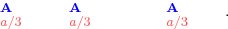• 2. If ${3 b \ge a > 2 b}$ then .

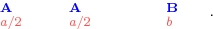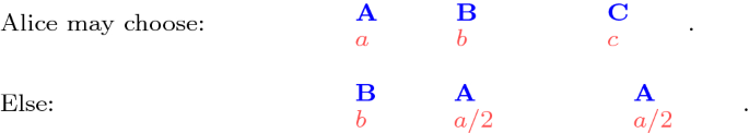
• 3. If ${2b \ge a > b+c}$ then play the sequential game below:

  

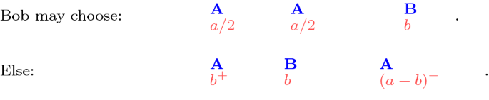
• 4. If ${a = b+c}$ then play the sequential game below:

  

• 5. If ${b + c > a}$ then

The income-subspaces of steps 1, 2, 3, 5 are covered by the two steps of Algorithm 1, but step 4 handles the set of incomes with $a=b+c$, which is not covered by Algorithm 1. I omitted it since it has a measure of zero, so it is not required for proving the existence of CE for almost all incomes.

Here is a proof that step 4 indeed implements a CE. First, note that the decreasing-prices condition is satisfied since $a>b>c$ and $2b > b+c = a$. By Lemma 4 no agent wants a dominated bundle. Bob has an unrelated bundle only in the second pixep, and he cannot afford it. It remains to check the unrelated bundles of Alice. Rename the items such that Alice’s best item is x. If Bob’s best item is not x, then Alice certainly plays BAA, since then she gets x plus another item. She obviously prefers this bundle to her only unrelated bundle, which is Bob’s single item. If Bob’s best item is x, then Alice effectively chooses between x (the ABC sequence) and yz (the BAA sequence). Whatever she chooses, she does not want the other (unrelated) bundle.

1.2 Theorem 6: Non-existence of CE with 5 goods

Babaioff et al. [11, Theorem 3.5] prove this theorem using a very similar example. With the transformation $A\rightarrow v, B\rightarrow w, C\rightarrow x, D\rightarrow y, E\rightarrow z$, the preferences implied by the numeric values in their Example 3.1 are:

• Alice: $vwz> vwy> vwx> vw> xyz> zyw> zxw> yxw> zyv> zxv> yxv> zy> zx> yx> zw> yw> xw> zv> yv> xv> z> y> x> w > v$.

• Bob: $wzy> wzx> wyz> vzy> vzx> vyx> zwv> ywv = zw> xwv = yw = zv> xw = yv> xv> xyz> vw> w> v> zy> zx> yx> z> y > x$.

The preferences are very similar, but they contain some indifferences between bundles (which do not affect the proof in any way). I just expressed the preferences as relations and without numbers, and also did not specify some relations that are irrelevant for the proof.

The main differences between the proofs are: (a) the proof in this paper uses only the fairness properties, so the impossibility result is stronger—it shows that even the fairness properties alone cannot be satisfied; (b) the proof in this paper is extended to any number $n \ge 2$ of agents.

Appendix 7: Allocations in different subgame-perfect equilibria

As noted in Sect. 5, some pixeps may have several different subgame-perfect equilibria, where only one of these SPE leads to a competitive equilibrium. Currently I do not have a general algorithm for determining the SPE that leads to a CE. However, the following lemma shows that, with strict preferences, the SPE selection affects only the prices and not the allocation.

Lemma 12

Suppose all agents have strict preferences. Then for any two subgame-perfect equilibria$Q_1,Q_2$of the same pixepS, the allocations$\mathbf{X}(S,Q_1)$and$\mathbf{X}(S,Q_2)$are the same.

Proof

The proof is by induction on n. For $n=1$ the claim is trivial. For $n>1$, assume the claim for all pixeps with $n-1$ agents, and consider two SPE of a pixep with n agents. Suppose w.l.o.g. that the first choice that differs between $Q_1$ and $Q_2$ is made by Alice. If Alice’s bundle in $Q_1$ differs from her bundle in $Q_2$, then (by strictness of preferences) she prefers one of these bundles; but then the other one cannot be a SPE. So Alice must get the same bundle in $Q_1$ and $Q_2$. Therefore, we can remove Alice from the sequence and remove her bundle from the set of items and get a new pixep with $n-1$ agents; by the induction assumption, all these agents have the same bundle in both equilibria. $\square$

Lemma 12 implies, in particular, that the resulting SPE allocation is CE-fair, since CE-fairness depends only on the allocation; the price-vector is used only as an evidence that the allocation is a CE.

In general, Lemma 12 does not hold for a sequential choice among several pixeps. For example, in the game “Alice chooses between AB and AC”, there are two SPEs with substantially different allocations. However, the lemma does hold in the specific sequential games in Algorithms 2 and 3:

• In Algorithm 2 there are only two agents: if Alice’s bundle is the same in both SPEs then obviously Bob’s bundle is the same too. The same is true in Algorithm 3 Range 4.

• In Algorithm 3 Range 5, Alice cannot be indifferent between her two choices, since in each choice she gets a different bundle (a singleton vs. a pair), and by assumption the preferences are strict. The same is true in Range 7. In Range 6, too, Alice’s choice is between a singleton and a pair, and Bob’s choice is between a pair and a singleton, so they cannot be indifferent. This means that a unique pixep is played in every SPE.

Lemma 12 does not hold with non-strict preferences. For example, suppose there are two items x, y, Alice is indifferent between them while Bob strictly prefers y. Then the picking-sequence AB has two SPEs—one in which Alice picks x and one in which she picks y—and they lead to two different allocations that are substantially different for Bob.

References

Abdulkadiroglu, A., & Sonmez, T. (1998). Random serial dictatorship and the core from random endowments in house allocation problems. Econometrica, 66(3), 689.
Anbarci, N. (1993). Noncooperative foundations of the area monotonic solution. The Quarterly Journal of Economics, 108(1), 245–258.
Anbarci, N. (2006). Finite alternating-move arbitration schemes and the equal area solution. Theory and decision, 61(1), 21–50.
Arrow, K. J., & Debreu, G. (1954). Existence of an equilibrium for a competitive economy. Econometrica, 22(3), 265–290.
Aumann, R. J. (1995). Backward induction and common knowledge of rationality. Games and Economic Behavior, 8(1), 6–19.
Aziz, H. (2015). Competitive equilibrium with equal incomes for allocation of indivisible objects. Operations Research Letters, 43(6), 622–624.
Aziz, H., Brandt, F., & Brill, M. (2013). The computational complexity of random serial dictatorship. Economics Letters, 121(3), 341–345.
Aziz, H., Goldberg, P., & Walsh, T. (2017). Equilibria in sequential allocation. In International conference on algorithmic decision theory (pp 270–283). Springer. arXiv preprint arXiv:1705.09444.
Aziz, H., Chan, H., & Li, B. (2019). Maxmin share fair allocation of indivisible chores to asymmetric agents. In Proceedings of AAMAS’19, IFAAMAS (pp. 1787–1789). arXiv preprint arXiv:1906.07602.
Babaioff, M., Nisan, N., & Talgam-Cohen, I. (2017). Competitive equilibria with indivisible goods and generic budgets. ArXiv preprint arXiv:1703.08150v1.
Babaioff, M., Nisan, N., & Talgam-Cohen, I. (2019a). Competitive equilibrium with generic budgets: Beyond additive. ArXiv preprint arXiv:1911.09992v1.
Babaioff, M., Nisan, N., & Talgam-Cohen, I. (2019b). Fair allocation through competitive equilibrium from generic incomes. In Proceedings of the conference on fairness, accountability, and transparency (pp. 180–180). ACM. arXiv preprint arXiv:1703.08150v2.
Bade, S. (2019). Random serial dictatorship: The one and only. Mathematics of Operations Research. https://doi.org/10.1287/moor.2019.0987.
Balinski, M., & Young, H. P. (1975). The quota method of apportionment. American Mathematical Monthly, 82(7), 701–730.
Barman, S., & Krishnamurthy, S. K. (2019). On the proximity of markets with integral equilibria. In Proceedings of AAAI’19 (pp. 1748–1755). AAAI Press. arXiv preprint arXiv:1811.08673.
Barman, S., Biswas, A., Krishnamurthy, S. K., & Narahari, Y. (2018). Groupwise maximin fair allocation of indivisible goods. In Proceedings of AAAI’18.
Bernheim, B. D. (1984). Rationalizable strategic behavior. Econometrica: Journal of the Econometric Society, 52, 1007–1028.
Biró, P., Kóczy, L. Á., & Sziklai, B. (2015). Fair apportionment in the view of the Venice Commission’s recommendation. Mathematical Social Sciences, 77, 32–41.
Bogomolnaia, A., Moulin, H., Sandomirskiy, F., & Yanovskaya, E. (2017). Competitive division of a mixed manna. Econometrica, 85(6), 1847–1871. arXiv:1702.00616.
Bouveret, S., & Lang, J. (2011). A general elicitation-free protocol for allocating indivisible goods. In Proceedings of IJCAI’11 (pp. 73–78). AAAI Press.
Bouveret, S., & Lemaître, M. (2016). Characterizing conflicts in fair division of indivisible goods using a scale of criteria. Autonomous Agents and Multi-Agent Systems, 30(2), 1–32.
Brainard, W. C., & Scarf, H. (2000). How to compute equilibrium prices in 1891. Technical report, Cowles Foundation for Research in Economics, Yale University.
Brams, S. J. (2007). Mathematics and democracy: Designing better voting and fair-division procedures (1st ed.). Princeton: Princeton University Press.
Brams, S. J., & Kaplan, T. R. (2004). Dividing the indivisible: Procedures for allocating cabinet ministries to political parties in a parliamentary system. Journal of Theoretical Politics, 16(2), 143–173.
Brânzei, S., Chen, Y., Deng, X., Filos-Ratsikas, A., Frederiksen, S. K., & Zhang, J. (2014). The fisher market game: Equilibrium and welfare. In Proceedings of AAAI ’14 (pp. 587–593). AAAI Press.
Brânzei, S., Hosseini, H., & Miltersen, P. (2015). Characterization and computation of equilibria for indivisible goods. In M. Hoefer (Ed.), Algorithmic game theory. Lecture notes in computer science (Vol. 9347, pp. 244–255). Berlin Heidelberg: Springer.
Brânzei, S., Lv, Y., & Mehta, R. (2016). To give or not to give: Fair division for single minded valuations. In Proceedings of IJCAI’16 (pp. 123–129). arXiv preprint arXiv:1602.09088.
Budish, E. (2011). The combinatorial assignment problem: Approximate competitive equilibrium from equal incomes. Journal of Political Economy, 119(6), 1061–1103.
Caragiannis, I., Kurokawa, D., Moulin, H., Procaccia, A. D., Shah, N., & Wang, J. (2019). The unreasonable fairness of maximum nash welfare. ACM Transactions on Economics and Computation (TEAC), 7(3), 12.
Cseh, Á., & Fleiner, T. (2018). The complexity of cake cutting with unequal shares. In Proceedings of SAGT’18 (pp. 19–30). Springer. arXiv preprint arXiv:1709.03152.
Deng, X., Papadimitriou, C., & Safra, S. (2003). On the complexity of price equilibria. Journal of Computer and System Sciences, 67(2), 311–324.
Erlich, S., Hazon, N., & Kraus, S. (2018). Negotiation strategies for agents with ordinal preferences. In Proceedings of IJCAI’18. arXiv preprint arXiv:1805.00913.
Farhadi, A., Ghodsi, M., Hajiaghayi, M. T., Lahaie, S., Pennock, D., Seddighin, M., et al. (2019). Fair allocation of indivisible goods to asymmetric agents. Journal of Artificial Intelligence Research, 64, 1–20.
Flis, J., Słomczyński, W., & Stolicki, D. (2020). Pot and ladle: A formula for estimating the distribution of seats under the Jefferson–D’hondt method. Public Choice, 182(1–2), 201–227.
Fudenberg, D., & Levine, D. K. (1993). Self-confirming equilibrium. Econometrica: Journal of the Econometric Society, 61, 523–545.
Garg, J., Kulkarni, P., & Kulkarni, R. (2020). Approximating Nash social welfare under submodular valuations through (un) matchings. In Proceedings of the fourteenth annual ACM-SIAM symposium on discrete algorithms (pp. 2673–2687). SIAM.
Heinen, T., Nguyen, N. T., & Rothe, J. (2015). Fairness and rank-weighted utilitarianism in resource allocation. In T. Walsh (Ed.), Algorithmic decision theory. Lecture notes in computer science (Vol. 9346, pp. 521–536). Berlin: Springer.
Kalinowski, T., Narodytska, N., & Walsh, T. (2013a). A social welfare optimal sequential allocation procedure. In Proceedings of IJCAI’13 (pp. 227–233). AAAI Press.
Kalinowski, T., Narodytska, N., Walsh, T., & Xia, L. (2013b). Strategic behavior when allocating indivisible goods sequentially. In Proceedings of AAAI’13. AAAI Press.
Kóczy, L. Á., & Sziklai, B. (2018). Bounds on malapportionment. Operations Research Letters, 46(3), 324–328.
Kóczy, L. Á., Biró, P., & Sziklai, B. (2017). US vs. European apportionment practices: The conflict between monotonicity and proportionality. In U. Endriss (Ed.), Trends in computational social choice (Chap. 16, pp. 309–325). AI Access.
Kohler, D. A., & Chandrasekaran, R. (1971). A class of sequential games. Operations Research, 19(2), 270–277.
Manea, M. (2009). Asymptotic ordinal inefficiency of random serial dictatorship. Theoretical Economics, 4(2), 165–197.
Maschler, M., Solan, E., & Zamir, S. (2013). Game theory. Cambridge: Cambridge University Press.
McKenzie, L. (1954). On equilibrium in Graham’s model of world trade and other competitive systems. Econometrica: Journal of the Econometric Society, 22, 147–161.
Moore, J., & Repullo, R. (1988). Subgame perfect implementation. Econometrica, 56(5), 1191–1220.
Moulin, H. (2004). Fair division and collective welfare. Cambridge: The MIT Press.
Nicolò, A., & Velez, R. A. (2017). Divide and compromise. Mathematical Social Sciences, 90, 100–110.
Nicolò, A., & Yu, Y. (2008). Strategic divide and choose. Games and Economic Behavior, 64(1), 268–289.
Nicolò, A., & Perea, Roberti P. (2012). Equal opportunity equivalence in land division. SERIEs: Journal of the Spanish Economic Association, 3(1–2), 133–142.
O’Leary, B., Grofman, B., & Elklit, J. (2005). Divisor methods for sequential portfolio allocation in multi-party executive bodies: Evidence from Northern Ireland and Denmark. American Journal of Political Science, 49(1), 198–211.
Othman, A., Papadimitriou, C., & Rubinstein, A. (2016). The complexity of fairness through equilibrium. ACM Transactions on Economics and Computation (TEAC), 4(4), 20.
Pukelsheim, F. (2017). Proportional representation. Berlin: Springer.
Reijnierse, J. H., & Potters, J. A. M. (1998). On finding an envy-free Pareto-optimal division. Mathematical Programming, 83(1–3), 291–311.
Segal-Halevi, E. (2018). Competitive equilibrium for almost all incomes. In Proceedings of AAMAS’18. arXiv preprint arXiv:1705.04212.
Segal-Halevi, E. (2019). Cake-cutting with different entitlements: How many cuts are needed? Journal of Mathematical Analysis and Applications, 480(1), 123,382. arXiv:1803.05470.
Segal-Halevi, E., Aziz, H., & Hassidim, A. (2017). Fair allocation based on diminishing differences. In Proceedings of the 26th international joint conference on artificial intelligence (pp. 1254–1261).
Segal-Halevi, E., & Suksompong, W. (2019). Democratic fair allocation of indivisible goods. Artificial Intelligence,277, 103167.
Segal-Halevi, E., & Sziklai, B. R. (2019). Monotonicity and competitive equilibrium in cake-cutting. Economic Theory, 68(2), 363–401.
Varian, H. R. (1974). Equity, envy, and efficiency. Journal of Economic Theory, 63–91.
Wald, A. (1935). Uber die eindeutige positive l osbarkeit der neuen produktionsgleichungen. Ergebnisse eines mathematischen Kolloquiums, 6, 1933–34.
Walras, L. (1874). Elements of pure economics. Translated from the French by William Jaffe at 1954.
Weller, D. (1985). Fair division of a measurable space. Journal of Mathematical Economics, 14(1), 5–17.
Young, H. P. (1974). An axiomatization of Borda’s rule. Journal of Economic Theory, 9(1), 43–52.
Zermelo, E. (1913). Über eine anwendung der mengenlehre auf die theorie des schachspiels. In Proceedings of the fifth international congress of mathematicians (Vol. 2, pp. 501–504). Cambridge University Press, Cambridge.
Acknowledgements
I am grateful to Inbal Talgam-Cohen, Noam Nisan, Moshe Babaioff, Fedor Sandomirskiy, lonza leggiera, Wolfram, and three anonymous reviewers of AAMAS 2018 for their very helpful comments. Special thanks are due to the anonymous referees of JAAMAS for their extraordinarily helpful reviews.
Author information
Authors and Affiliations
Corresponding author
Additional information
Publisher's Note
Springer Nature remains neutral with regard to jurisdictional claims in published maps and institutional affiliations.
A preliminary version appeared in the proceedings of AAMAS 2018. That version contained a severe error—the algorithm for 4 goods and 3 agents had a bug. I am very grateful to an anonymous referee for a comment that lead to revealing this bug (as well as hundreds of other helpful comments). In fact, there is an impossibility result for this case, which is presented in this paper. Moreover, this paper extends the results to allocation of indivisible chores (bads). Additionally, it proves new fairness criteria satisfied by competitive equilibria.