A new structural approach to isoparametric hypersurfaces in spheres

Abstract

In this paper we show that the long-standing problem of classifying all isoparametric hypersurfaces in spheres with six different principal curvatures is still not complete. Moreover, we develop a structural approach that may be helpful for such a classification. Instead of working with the isoparametric hypersurface family in the sphere, we consider the associated Lagrangian submanifold of the real Grassmannian of oriented 2-planes in ${\mathbb {R}}^{n+2}$. We obtain new geometric insights into classical invariants and identities in terms of the geometry of the Lagrangian submanifold.

1 Introduction

Originally, isoparametric hypersurfaces were defined to be the level sets of isoparametric functions, i.e., functions on a real space form whose gradient norm and Laplacian are constant on the level sets. This condition translates into the equivalent geometric condition that the principal curvatures of the hypersurfaces are constant. The classifications of isoparametric hypersurfaces in the cases where the ambient space is Euclidean or hyperbolic space were settled soon by Somigliana [28], Segre [26], and Cartan [2,3,4,5]. In contrast, when the ambient space is a sphere, the number g of distinct principal curvatures can be greater than two, which makes a classification much more difficult. In this paper we henceforth consider the case where the ambient space is a sphere.

Cartan [2,3,4,5] classified isoparametric hypersurfaces with $g\le 3$ and showed that they are all homogeneous, i.e., orbits of isometric group actions on $\mathbb {S}^{n+1}$. The problem was picked up again by Münzner [20, 21] who showed that the number of distinct principal curvatures g can be only 1, 2, 3, 4, or 6 and gave restrictions for the multiplicities as well. The possible multiplicities of the curvature distributions were classified in [1, 21, 29] and coincide with the multiplicities in the known examples. The situation in the case $g = 4$ is more complex since there exist infinitely many isoparametric hypersurfaces and infinitely many of them are inhomogeneous—see Cecil [6] or Thorbergsson [31] for very good recent surveys of this case. In the case $g=6$ all multiplicities m coincide and equal either 1 or 2, and precisely two homogeneous examples are known. Dorfmeister and Neher [9] conjectured that all isoparametric hypersurfaces with $g=6$ are homogeneous and in the same paper settled this conjecture in affirmative for $m=1$. In the remaining open case $m = 2$, Miyaoka [17, 19] proposed how to establish homogeneity. However, in Appendix we give a counterexample to one crucial proposition in [17, 19]. Thus, the classification of isoparametric hypersurfaces with $g=6$ and $m=2$ is still open.

In the present paper we develop a new structural approach to isoparametric hypersurfaces in spheres, unifying many of the known geometric properties.

The basic idea is as follows. Instead of working with the family of parallel surfaces $F_t:M^n\rightarrow \mathbb {S}^{n+1}$, with normal field $\nu _t\in \Gamma (\nu M^n)$, one considers the associated submanifold of the real Grassmannian of oriented 2-planes in ${\mathbb {R}}^{n+2}$

$$\begin{aligned} {\mathfrak {L}}: M^n\rightarrow Gr^{+}_2({\mathbb {R}}^{n+2})\subset \mathbb {CP}^{n+1} \end{aligned}$$

by sending $p\in M^n$ to the 2-plane spanned by $F_t(p)$ and $\nu _t(p)$. One easily sees that ${\mathfrak {L}}$ does not depend on t, and in [24, 25] it was observed that for any submanifold of $\mathbb {S}^{n+1}$ the associated submanifold ${\mathfrak {L}}(M)\subset Gr^{+}_2({\mathbb {R}}^{n+2})$ is Lagrangian with respect to the natural symplectic structure.

We endow the Lagrangian submanifold with a set of invariants which arise naturally: the metric induced via the canonical Kähler metric $g_{Q}$ on $Gr^{+}_2({\mathbb {R}}^{n+2})$, i.e., ${\hat{g}}={\mathfrak {L}}^{*}g_{Q}$; the symmetric tensor $\alpha$

$$\begin{aligned} \alpha (X,Y,Z)=g_t\left( \left( \nabla _X^tA_t\right) Y,Z\right) , \end{aligned}$$

where $A_t$ denotes the shape operator of $F_t$ with respect to $\nu _t$, $X,Y,Z\in \Gamma (TM)$; and

$$\begin{aligned} B\otimes B^{-1}:=B_t\otimes B_t^{-1}, \end{aligned}$$

where $B_{t}:\Gamma (TM)\rightarrow \Gamma (TM)\otimes \mathbb {C}$ is defined via The set of invariants $({\hat{g}},\alpha ,B\otimes B^{-1})$ depends only on the isoparametric family it is contained in.

The tensor $\alpha$ is one of the fundamental invariants used in the previous classification approaches though usually encoded in some much less invariant Maurer–Cartan forms $\Lambda$. The really interesting fact is that $\alpha$ coincides—up to a factor of two—with the second fundamental form of the Lagrangian submanifold, which gives a new, geometric interpretation for this important tensor.

Theorem A

The tensor $\alpha$ coincides, up to a factor of two, with the second fundamental form of the Lagrangian submanifold.

The introduction of the set of invariants $({\hat{g}},\alpha ,B\otimes B^{-1})$ is justified by the fact that they allow us to formulate all relevant identities in a compact way.

For the theory of isoparametric hypersurfaces in spheres, the so-called Weyl identities are of utmost importance. The classical Weyl identities depend on several indices. In terms of the invariants described above, these multiple identities unify into one tensor identity, see Theorem 3.8.

Another set of equations which can easily be formulated in terms of $\alpha$ are the symmetry identities: The pullback of $\alpha$ under the reflections through each of the focal manifolds coincides with the negative of $\alpha$. So far, all these considerations are completely general.

Below we restrict ourselves to the case $g=6$, and give several reformulations for homogeneity. Here, we just mention the following reformulation, which relates homogeneity to geometric properties of the Lagrangian submanifold. For other reformulations see Sect. 4.

Theorem B

The homogeneity of isoparametric hypersurfaces with $g=6$ different principal curvatures is equivalent to

$$\begin{aligned} R(\pi _iX,\pi _{i+3}Y,\pi _{i+3}Y,\pi _iX)=0,\,\forall i\in \left\{ 1,\ldots ,6\right\} , \,\forall X,Y\in \Gamma (TM) \end{aligned}$$

where R is the curvature tensor of the Lagrangian submanifold ${\mathfrak {L}}(M^n)$.

The previous theorem thus reduces the classification of isoparametric hypersurfaces with $g=6$ to a geometric problem for Lagrangian submanifolds of the complex quadric. We hope that our approach might finally lead to a classification of isoparametric hypersurfaces with $g=6$. Note that up till now, for the classification of isoparametric hypersurfaces with $g=6$, there exists only one approach suggested by Dorfmeister and Neher [9]. However, for the remaining case $m=2$, the underlying algebraic problem turned out to be very hard, and no one was so far able to carry out their approach for $m=2$. Therefore, a new approach seems to be needed.

Using this structural approach we can reprove many of the classical results. Most proofs become simpler and render greater geometric insight.

This paper is organized as follows: In Sect. 1 we recall a few preliminary definitions and give a survey of results needed later on. In Sect.  2 we carry out the translation from the isoparametric hypersurface family in the sphere to the Lagrangian submanifold of the real Grassmannian of oriented 2-planes in ${\mathbb {R}}^{n+2}$. In particular, we introduce the set $({\hat{g}},\alpha ,B\otimes B^{-1})$ of structural invariants. Sect. 3 deals with the fundamental submanifold equations of the Lagrangian submanifold. Moreover, we derive the Weyl identities and the symmetry identities. In Sect. 4 we give several equivalent formulations of homogeneity. Finally, we provide a counterexample to one crucial proposition in Miyaoka’s [17, 19] approach in Appendix.

2 Preliminaries

In this section we gather the definitions and tools which we will need later on. Throughout this paper, let M be a connected, smooth manifold of dimension n.

2.1 Isoparametric hypersurface

We start by recalling the definition of an isoparametric hypersurface in a sphere.

Definition 1.1

An embedding $F_{0}:{M}\hookrightarrow \mathbb {S}^{n+1}$ together with a distinguished unit normal vector field $\nu _0\in \Gamma (\nu M)$ is called an isoparametric hypersurface in $\mathbb {S}^{n+1}$ if and only if the principal curvature functions are constant.

The data of an isoparametric hypersurface are g, the number of distinct principal curvatures, and $m_j$ ($1\le j\le g$), the multiplicities of the curvature distributions.

Below we assume that $(F_0,\nu _0)$ constitutes an isoparametric hypersurface in $\mathbb {S}^{n+1}$. Let $A_0$ be the shape operator of $F_0$ with respect to $\nu _0$. We denote the g different eigenvalues of $A_0$, i.e., the principal curvature functions, by $\lambda _{j}(0)$. By assumption the $\lambda _j(0)$ are constant on M. Without loss of generality, we assume $\lambda _1(0)>\cdots >\lambda _g(0)$ and define $\theta _j\in \left( -\frac{\pi }{2},\frac{\pi }{2}\right)$ such that $\lambda _j(0)=\cot (\theta _j)$.

We denote the curvature distribution associated with $\lambda _j(0)$ by $D_j$, i.e., we have $D_j=\text{ Eig }(A_0,\lambda _j(0))$. Furthermore, we let $\pi _j:TM\rightarrow D_j$ be the orthogonal projection into $D_j$. Note that we have $m_j=\dim D_j$. The following lemma is due to Münzner [20].

Lemma 1.2

([20]) The curvature distribution $D_j$ is integrable, and the leaves are small spheres in $\mathbb {S}^{n+1}$ with curvature $1+\cot ^2(\theta _j)$. These spheres are totally geodesic submanifolds of M.

2.2 Parallel surfaces

Isoparametric hypersurfaces always come along as families of isoparametric hypersurfaces; namely, ‘almost all’ parallel surfaces of a given isoparametric hypersurface are also isoparametric hypersurfaces.

In what follows let $F_{0}:{M}\hookrightarrow \mathbb {S}^{n+1}$ together with a distinguished normal vector field $\nu _0$ be a fixed isoparametric hypersurface. By slight abuse of notation we also call the image $F_0(M)$ an isoparametric hypersurface. We consider the parallel surface $F_{t}: M\hookrightarrow \mathbb {S}^{n+1}$ with signed distance t to $F_0$. It is given by

$$\begin{aligned} p\mapsto F_t(p):=\exp _{F_0(p)}(t\nu _{0\vert p})=\cos (t)F_0(p)+\sin (t)\nu _{0\vert p}, \end{aligned}$$

endowed with the orientation

$$\begin{aligned} \nu _{t}(p)=-\sin (t)F_{0}(p)+\cos (t){\nu _{0}}_{\vert _p}. \end{aligned}$$

The map $F_t$ induces the following data on M: the Riemannian metric $g_t=F_t^{*}\left\langle \cdot ,\cdot \right\rangle _{\mathbb {S}^{n+1}}$, the associated Levi-Civita connection $\nabla ^t$, and the shape operator $A_t$ of the submanifold $(M,g_{t})\subset (\mathbb {S}^{n+1},\left\langle \cdot ,\cdot \right\rangle _{\mathbb {S}^{n+1}})$ with respect to $\nu _t$.

In the next lemma we express $A_t$ in terms of $A_0$ since this will be needed later on.

Lemma 1.3

In terms of $A_0$ the shape operator $A_t$ is given by

where in the cases $t=\theta _{j}+\ell \pi$, $\ell \in \mathbb {Z}_2$, the operator $A_{t}$ is defined on $TM\!\setminus \! D_j$.

Proof

Since

Eq. (2) implies

(1)

whence the claim. $\square$

We will now make sense of the statement that ‘almost all’ parallel surfaces of a given isoparametric hypersurface are also isoparametric hypersurfaces. Using the identity $d \nu _{0}=-dF_{0}A_{0}$ we get

(2)

and hence ${\text {rk}}(dF_{t\vert p})=n$ if $t\ne \theta _j\,\,\text{ mod }\,\pi$ and ${\text {rk}}(dF_{t\vert p})=n-m_j$ otherwise.

If $t\ne \theta _j\,\,\text{ mod }\,\pi$, the parallel surface $F_t(M)$ is again an isoparametric hypersurface. Lemma 1.3 implies that the principal curvatures of $F_t(M)$ are given by $\lambda _j(t)=\cot (\theta _j-t)$.

If $t=\theta _j\,\,\text{ mod }\,\pi$, the $m_j$-dimensional eigenspace $D_j(p)$ is the kernel of $dF_{t\vert p}$ for every $p\in M$. In other words, the leaf $L_j(p)$ of $D_j$ through p is focalized into the point $\overline{p}=F_{\theta _j}(p)$. Hence, $M_{j}:=F_{\theta _j}(M)$ is the so-called focal submanifold of dimension $(n-m_j)$.

Summarizing the previous considerations we get

$$\begin{aligned} F_0\,\,\text{ isoparametric }\Rightarrow F_t \,\,\,\text{ is }\,\,\left\{ \begin{array}{ll} \text{ isoparametric },&{}\quad \text{ if } \cot (t)\notin \text{ spec }(A_0); \\ \text{ submersion } \text{ onto } \text{ a } \text{ focal } \text{ manifold },&{}\quad \text{ otherwise. } \end{array}\right. \end{aligned}$$

Finally, it is important to remark that all the hypersurfaces in a family of parallel isoparametric hypersurfaces have the same focal submanifolds. It is easily shown, see, e.g., [20], that there are exactly two focal submanifolds.

2.3 Spectrum of the focal shape operators

Using identity (2), Münzner [20] proved that for $t=\theta _j\,\,\text{ mod }\,\pi$ the spectrum of $A_{t\vert \nu _p}$ is independent of $\nu \in \nu M_{j}$ and $p\in M_{j}$ and is given by

$$\begin{aligned} \text{ spec }(A_{t\vert \nu _p})=\left\{ \cot \big ((i-j)\pi /g \big )\, \vert \, i\in \left\{ 1,\ldots ,g\right\} ,\, i\ne j\right\} . \end{aligned}$$

(3)

Thus, for each $p\in M_{j}$ and each pair of orthonormal vectors $v_1,v_2\in \nu _p M_{j}$ the family

$$\begin{aligned} L(s)=\cos (s)A_{t\vert v_1}+\sin (s)A_{t\vert v_2},\,s\in {\mathbb {R}}, \end{aligned}$$

is isospectral. We will henceforth refer to L(s) as the isospectral family at $p\in M_{j,\ell }$ with respect to $(v_1,v_2)\in \nu _p M_{j}$.

The fact that the spectrum of the focal shape operator of the focal submanifold is independent of $\nu \in \nu M_{j}$ and $p\in M_{j}$ implies that the eigenvalues $\lambda _k(0)$, $k\in \left\{ 1,\ldots ,g\right\}$, are of the form $\lambda _k(0)=\cot (\phi +(k-1)\pi /g),$ with $0<\phi <\pi /g$. Thus, $\theta _k=\phi +(k-1)\pi /g$ modulo $\pi$.

The parameter $\phi$ in the formula for $\theta _j$ encodes the position of $F_{0}$ in the isoparametric family. We shall choose the initial hypersurface such that $\phi =\theta _1=\frac{\pi }{2g}$. Thus, the initial isoparametric hypersurface is the one which lies in the middle of the focal submanifolds $F_{-\pi /2g}(M)$ and $F_{\pi /2g}(M)$.

Using that the spectrum of $A_{t \nu _p}$ is independent of $\nu \in \nu M_{j}$, Münzner proved that the multiplicities satisfy the equation

$$\begin{aligned} m_{i}=m_{i+2}, i\in \mathbb {Z}_g. \end{aligned}$$

Therefore, at most two distinct values for the multiplicities exist. They will henceforth be referred to as $m_1$ and $m_2$. If all multiplicities coincide, which is, for example, the case if g is odd, their common value is denoted by m.

2.4 Global structure

The global situation is as follows:

$$\begin{aligned} \mathfrak {F}=\left\{ F_t(M)\,|\,t\in \left[ -\pi /2g,\pi /2g\right] \right\} \end{aligned}$$

is a singular Riemannian foliation, $F_t(M)$ are isoparametric hypersurfaces for all $t\in \left( -\pi /2g,\pi /2g\right)$, $F_{-\pi /2g}(M)$ and $F_{\pi /2g}(M)$ are submanifolds of codimension at least two in $\mathbb {S}^{n+1}$. Each normal geodesic $\gamma$ intersects the focal submanifolds at times $t=(2j+1)\pi /2g$, $j\in \mathbb {Z}$, alternating between the two focal submanifolds $M_+:=F_{-\pi /2g}(M)$ and $M_-:=F_{\pi /2g}(M)$. The regular set $\mathcal {R}$ is the set of times $t\in {\mathbb {R}}$ such that $\gamma (t)$ is not a focal point,

$$\begin{aligned} \mathcal {R}=\left\{ t\in {\mathbb {R}}\,|\,\not \exists \,j\in \mathbb {Z}\,\, \text{ with }\,\,t=(2j+1)\pi /2g\right\} . \end{aligned}$$

Any fixed isoparametric hypersurface $F_{t_0}(M)\in \mathfrak {F}$ coincides with either of the tubes $\text{ Tube }_{d_+}(M_+)$ and $\text{ Tube }_{d_-}(M_-)$ of radius $d_+$ and $d_-$, respectively, where $d_{\pm }$ denotes the distance of $M_{\pm }$ to $F_{t_0}(M)$. Thus, each normal geodesic intersects a given isoparametric hypersurface $F_{t_0}(M)$ exactly 2g times before it closes. Furthermore, the focal set of each isoparametric hypersurface $F_{t_0}(M)$ is exactly the union of $M_+$ and $M_-$.

Figure 1 shows the sketch a normal geodesic in the case $g=3$. It intersects each isoparametric hypersurface exactly six times before it closes. The intersection points with one fixed isoparametric hypersurface are marked by solid points.

Fig. 1

Global picture for $g=3$

2.5 Topology

Each isoparametric hypersurface $F_{t_0}(M)$ separates the sphere $\mathbb {S}^{n+1}$ into two connected components $B_+$ and $B_-$, i.e., $F_{t_0}(M)=B_+\cap B_-$ and $\mathbb {S}^{n+1}=B_+\cup B_-$, such that these components are disk bundles over the focal manifolds. Assume without loss of generality that $M_+$ has codimension $m_1+1$ and that $M_-$ has codimension $m_2+1$. Thus, we have the disk bundles

$$\begin{aligned} D_{\pm }\rightarrow B_{\pm }\rightarrow M_{\pm }, \end{aligned}$$

where the fibers $D_+$ and $D_-$ have dimensions $m_1+1$ and $m_2+1$, respectively.

This topological fact was used in the papers [1, 21] and [29] to classify the number of distinct principal curvatures and their possible multiplicities.

2.6 Classification results

In Table 1 the known classification results for isoparametric hypersurfaces in spheres with g different principal curvatures are summarized. Recall that if the multiplicities $m_1$ and $m_2$ coincide their common value is denoted by m.

Table 1 Classification results of isoparametric hypersurfaces in spheres

The classification of isoparametric hypersurfaces with $g\le 3$ is due to Cartan [2,3,4,5].

While all isoparametric hypersurfaces with $g\le 3$ are homogeneous, the situation in the case $g =4$ is more complex since there exist infinitely many isoparametric hypersurfaces and infinitely many of them are inhomogeneous.

Ferus et al. [10] used representations of Clifford algebras to produce a class of isoparametric families with four principal curvatures, the so-called isoparametric hypersurfaces of FKM type. Stolz [29] proved that the multiplicities of an isoparametric hypersurface with four principal curvatures must coincide with those in the known examples of FKM type or two homogeneous exceptions, namely $(m_1,m_2)=(2,2)$ or (4, 5). Cecil et al. [7] proved that if the multiplicities $(m_1,m_2)$ satisfy $m_2\ge 2m_1-1$, then the isoparametric hypersurfaces are necessarily of FKM type. Thus, the cases $(m_1,m_2)=(4,5), (3,4), (6,9)$, and (7, 8) were left, which were successively classified by Chi, see [8] and the references therein. For a detailed exposition to the cases $g=4$ we refer the reader to the surveys by Cecil [6] and Thorbergsson [31].

We postpone a detailed exposition of the case $g=6$ to Sect. 4, since in order to do so, we make use of results presented in Sects. 2 and 3.

3 The Lagrangian submanifold model and its structural invariants

As already discussed in Sect. , isoparametric hypersurfaces always come along as families of isoparametric hypersurfaces. To each family of isoparametric hypersurfaces, we associate a Lagrangian submanifold of the complex quadric. Thus, instead of working with a family of hypersurfaces, we can henceforth work with only one submanifold. For this submanifold we introduce a set of invariants $({\hat{g}},\alpha ,B\otimes B^{-1})$ and endow them with a geometric meaning.

This section is structured as follows: In the first subsection we recall the definition and basic properties of the complex quadric. The construction of the Lagrangian submanifold of the complex quadric is explained in the second subsection. Finally, we introduce the set of invariants in the third subsection. Throughout this section let $X,Y,Z,W\in \Gamma (TM)$.

3.1 The complex quadric

In this subsection we give a very brief introduction to the complex quadric. We just cover those definitions and facts needed later on. For a detailed exposition we refer the reader to the book [11] of Gasqui and Goldschmidt which we use as a reference.

We write $\left\langle \cdot ,\cdot \right\rangle _{\mathbb {C}^{n+2}}$ and $\left\langle \cdot ,\cdot \right\rangle _{h}$ for the standard complex bilinear and the standard hermitian inner product of $\mathbb {C}^{n+2}$, respectively.

Definition 2.1

The complex quadric is the complex hypersurface of $\mathbb {CP}^{n+1}$ given by

$$\begin{aligned} Q_n=\left\{ \left[ z\right] \in \mathbb {CP}^{n+1}\,|\,z_0^2 +\cdots +z_{n+1}^2=0\right\} , \end{aligned}$$

where $z=(z_0,\ldots ,z_{n+1})$ denote the standard coordinates of $\mathbb {C}^{n+2}$.

Clearly, the complex quadric $Q_n$ may also be described by

$$\begin{aligned} Q_n=\left\{ \pi (z)\vert \, z\in \mathbb {S}^{2n+3}, \left\langle z,z\right\rangle _{\mathbb {C}^{n+2}}=0\right\} , \end{aligned}$$

where $\pi :\mathbb {C}^{n+2}\setminus \left\{ 0\right\} \rightarrow \mathbb {CP}^{n+1}$ is the natural projection, where $\mathbb {S}^{2n+3}\subset \mathbb {C}^{n+2}$ is endowed with the Riemannian metric induced by $\langle \cdot ,\cdot \rangle _{{\mathbb {R}}}=\text{ Re }\langle \cdot ,\cdot \rangle$ on $\mathbb {C}^{n+2}$.

Another well-known fact is that the complex quadric $Q_n$ is diffeomorphic to the real Grassmannian $Gr^{+}_2({\mathbb {R}}^{n+2})$ of oriented 2-planes in ${\mathbb {R}}^{n+2}$. From now on we shall use this identification whenever convenient.

The remaining part of this subsection aims at describing the curvature tensor of Q. In order to do so, we first have to introduce some notation.

Let $g_Q$ denote the Kähler metric on $Q_n$ induced from the Fubini-Study metric $g_{FS}$ on $\mathbb {CP}^{n+1}$ (of constant holomorphic curvature 4) by the inclusion map $\iota :Q_n\rightarrow \mathbb {CP}^{n+1}$, i.e., $g_Q=\iota ^{*}g_{FS}$. The associated Levi-Civita connection of $Q_n$ is denoted by $\nabla ^Q$. For both $\mathbb {CP}^{n+1}$ and $Q_n$, the complex structure shall be called J and the associated Kähler form $\omega$.

It is well known that the projection $\pi :\mathbb {S}^{2n+3}\rightarrow \mathbb {CP}^{n+1}$ is a Riemannian submersion and that the map $d\pi :H_z\rightarrow T_{\pi (z)}\mathbb {CP}^{n+1}$ is an isometry, where

$$\begin{aligned} H_z=\left\{ u\in \mathbb {C}^{n+2}\vert \, \left\langle z,u\right\rangle _{\mathbb {C}^{n+2}}=0\right\} . \end{aligned}$$

For a point $z\in \mathbb {S}^{2n+3}$ which satisfies $\left\langle z,z\right\rangle _{\mathbb {C}^{n+2}}=0$ we get an isometry $d\pi :H_z^{'}\rightarrow T_{\pi (z)}Q$, where $H_z^{'}$ is the subspace of $H_z$ defined by

$$\begin{aligned} H_z^{'}=\left\{ u\in \mathbb {C}^{n+2}\vert \, \left\langle z,u\right\rangle _{\mathbb {C}^{n+2}}=0,\, \left\langle z,u\right\rangle _h=0\right\} . \end{aligned}$$

(4)

The preceding considerations allow us to identify the tangent space $T_qQ^n$ of the complex quadric at a given point $q\in Q^n$ with $\mathbb {C}^n$. Then the complex structure on $T_qQ^n$ is given by multiplication by i on $\mathbb {C}^n$, and the Kähler metric $g_Q$ corresponds to the real part of the standard Hermitian inner product on $\mathbb {C}^n$. Below we shall use this identification whenever convenient.

Gathering the preceding information and carrying out a straightforward calculation, one obtains the following lemma.

Lemma 2.2

([11]) The Riemann curvature tensor of the quadric $Q^n$ is given by

where $q(\,\cdot \,,\,\cdot \,)=\langle \,\cdot \,,\,\cdot \,\rangle _{\mathbb {C}^{n+2}}$ and $\overline{q}(\,\cdot \,,\,\cdot \,)=\overline{\langle \,\cdot \,,\,\cdot \,\rangle }_{\mathbb {C}^{n+2}}$.

For the convenience of the reader we recall the definition of the Kulkarni–Nomizu product.

Definition 2.3

The Kulkarni–Nomizu product

• (i) of two symmetric (2, 0)-tensors $h_1$ and $h_2$ is the (4, 0)-tensor given by

  

• (ii) of the skew-symmetric form $\omega$ with itself is given by

  

3.2 From families of isoparametric hypersurfaces to a Lagrangian submanifold of the complex quadric

In Palmer [24, 25] showed that every oriented, immersed hypersurface in the sphere naturally leads to a Lagrangian submanifold of the complex quadric. We will apply this construction to isoparametric hypersurfaces in spheres. In particular, we prove that every isoparametric hypersurface of a given family of isoparametric hypersurfaces leads to the same Lagrangian submanifold of the sphere.

We start by recalling the definition of the Stiefel manifold.

Definition 2.4

The Stiefel manifold is given by

$$\begin{aligned} St_2({\mathbb {R}}^{n+2})=\left\{ (v,w)\in \mathbb {S}^{n+1}\times \mathbb {S}^{n+1}\vert \, \left\langle v,w\right\rangle _{{\mathbb {R}}^{n+2}}=0\right\} , \end{aligned}$$

where $\left\langle \cdot ,\cdot \right\rangle _{{\mathbb {R}}^{n+2}}$ denotes the standard metric of ${\mathbb {R}}^{n+2}$.

Clearly, the Stiefel manifold can be identified with

$$\begin{aligned} \left\{ z\in \mathbb {S}^{2n+3}\vert \, \left\langle z,z\right\rangle _{\mathbb {C}^{n+2}}=0\right\} \subset \mathbb {S}^{2n+3} \end{aligned}$$

by the map $(v,w)\mapsto \tfrac{1}{\sqrt{2}} (v+iw)\in \mathbb {S}^{2n+3}$. Consequently, $\pi (St_2({\mathbb {R}}^{n+2}))=Q_n$ and it follows easily that the projection $\pi :\,St_2({\mathbb {R}}^{n+2})\rightarrow Q_n\subset \mathbb {CP}^{n+1}$ is a Riemannian submersion.

In order to associate a Lagrangian submanifold with an isoparametric hypersurface $(F_t,\nu _t)$, we first lift the embeddings $F_t$ to the Stiefel manifold $St_2({\mathbb {R}}^{n+2})$ and then concatenate this map with the projection onto the Grassmannian $\text{ Gr }_2^+({\mathbb {R}}^{n+2})$. For $t\ne \theta _j$ we define the map ${\hat{F}}_{t}$ by

$$\begin{aligned} {\hat{F}}_{t}:\,M\rightarrow St_2\left( {\mathbb {R}}^{n+2}\right) ,\quad p\mapsto {\hat{F}}_{t}(p):=\tfrac{1}{\sqrt{2}}\left( F_{t}(p)+i{\nu _{t}}_{\vert _p}\right) . \end{aligned}$$

Furthermore, we introduce the map ${\mathfrak {L}}$ by

$$\begin{aligned} {\mathfrak {L}}:=\pi \circ {\hat{F}}_{t}:M\rightarrow Q_n,\quad p\mapsto [{\hat{F}}_0(p)]. \end{aligned}$$

Fig. 2

The Lagrangian immersion ${\mathfrak {L}}$

Note that ${\mathfrak {L}}(p)$ is by construction the oriented 2-plane in ${\mathbb {R}}^{n+2}$ which is spanned by ${F}_{t}(p)$ and $\nu _{t|p}.$ Since we have $\hat{F_t}=e^{-it}{\hat{F}}_0$, the immersion ${\mathfrak {L}}$ does not depend on the parameter t. Thus, we obtain the following lemma (Fig. 2).

Lemma 2.5

Let a family of isoparametric hypersurfaces in a sphere be given. For each isoparametric hypersurface in this family we obtain the same immersion ${\mathfrak {L}}$.

As already mentioned above, the next result was first proved by Palmer [24, 25]. For convenience of the reader we reprove this result.

Proposition 2.6

([24, 25]) The map ${\mathfrak {L}}:=\pi \circ {\hat{F}}_{t}:M\rightarrow Q_n$, $p\mapsto [{\hat{F}}_0(p)]$, is a Lagrangian immersion with normal vector field $N_Z=\pm i\,d{\hat{F}}_0Z$, where $Z\in TM.$

Proof

Using the identity $d\nu _{t}=-dF_{t}A_{t}$, we obtain

for all $t\in {\mathbb {R}}$. Thus, we get

$$\begin{aligned} \hat{F_t}^{*}\omega (X,Y)&=g_Q(J d\hat{F_t}X,d\hat{F_t}Y)=\text{ Re }{\left\langle id{\hat{F}}_{0}X,d{\hat{F}}_{0}Y\right\rangle }_h\\&=\tfrac{1}{2} \big (g_0(A_{0}X,Y)+g_0(X,-A_{0}Y)\big )=0, \end{aligned}$$

which proves our claim. $\square$

Lemma 2.7

${\hat{F}}_{t}(M)$ is horizontal with respect to the projection $\pi :St_2({\mathbb {R}}^{n+2})\rightarrow Q_n.$

Proof

For any $p\in M$

$$\begin{aligned} \text{ Im }(dF_{0\vert p})\perp {\text {span}}\left\{ F_{0}(p),\nu _{0\vert p}\right\} \end{aligned}$$

in ${\mathbb {R}}^{n+1}$. Thus, identities (2) and (1) imply

$$\begin{aligned} \text{ Im }(d{\hat{F}}_{t\vert p})\perp \mathbb {C}{\hat{F}}_{t}(p)\oplus \mathbb {C}\overline{{\hat{F}}_{t}(p)} \end{aligned}$$

in $\mathbb {C}^{n+1}$. The claim now follows from (4). $\square$

Remark 2.8

The above construction was used by Ma and Ohnita [22] to classify compact homogeneous Lagrangian submanifolds in complex hyperquadrics.

3.3 A set of invariants of the Lagrangian submanifold

In this subsection we introduce a set of invariants for the Lagrangian submanifold of the complex quadric. Furthermore, for each of these invariants, we establish some basic properties.

3.3.1 The metric ${\hat{g}}$

We endow the Lagrangian submanifold with the natural metric, i.e., the Riemannian metric ${\hat{g}}$ on M induced from $\left\langle \cdot ,\cdot \right\rangle _h$ by ${\hat{F}}_{t}$. This metric is given by

$$\begin{aligned} {\hat{g}}=\text{ Re } ({\hat{F}}_{t}^{*}\left\langle \cdot ,\cdot \right\rangle _h). \end{aligned}$$

Lemma 2.7 asserts that the Riemannian metric ${\hat{g}}$ is induced from $g_Q$ by ${\mathfrak {L}}$. In particular, the metric ${\hat{g}}$ is independent of t.

In the next two lemmas we relate ${\hat{g}}$ and the associated Levi-Civita connection to $g_t$ and $\nabla ^t$, respectively.

Lemma 2.9

For each $p\in M$ and all $t\in {\mathbb {R}}$ we have

In particular, ${\hat{g}}$ is independent of t.

Proof

Since ${\hat{F}}_{t}=e^{-it}{\hat{F}}_{0}$ we have

$$\begin{aligned} d\hat{{F}}_{t}=e^{-it}d{\hat{F}}_{0}. \end{aligned}$$

By the definition of ${\hat{g}}$ and the preceding identity this gives

$$\begin{aligned} {\hat{g}}(X,Y)=\text{ Re }\left\langle d{\hat{F}}_{t}X,d{\hat{F}}_{t}Y\right\rangle _h=\text{ Re }\left\langle d{\hat{F}}_{0}X,d{\hat{F}}_{0}Y\right\rangle _h, \end{aligned}$$

for all $X,Y\in \Gamma (TM)$, and therefore

$\square$

Remark 2.10

The induced metric ${\hat{g}}$ is the arithmetic mean of some $g_{t}$:

Let $\phi \in \left( 0,\pi /2g\right)$ be given and define the arc $\xi _k$ for $k\in \mathbb {N}$ by $\xi _k=\phi +k\pi /2g$. Then ${\hat{g}}=\frac{1}{2}(g_{\phi }+g_{\phi +\pi /2})$ and ${\hat{g}}=\frac{1}{2g}\sum _{k=0}^{2g-1}{g_{\xi _k}}$.

We denote the Levi-Civita connection associated with ${\hat{g}}$ by $\nabla$. The next lemma relates $\nabla$ and $\nabla ^t$.

Lemma 2.11

The connections $\nabla$ and $\nabla ^{t}$ are related by

Proof

The Koszul formula yields

$$\begin{aligned} 2{\hat{g}}(\nabla _XY,Z)=\left( \nabla ^t_X{\hat{g}}\right) (Y,Z) +\left( \nabla ^t_Y{\hat{g}}\right) (X,Z)-\left( \nabla ^t_Z{\hat{g}}\right) (X,Y)+2{\hat{g}}\left( \nabla ^t_XY,Z\right) . \end{aligned}$$

By Lemma 2.9 we get

$$\begin{aligned} \left( \nabla ^t_{X_1}{\hat{g}}\right) (X_2,X_3)=\tfrac{1}{2}g_t \left( \big (\left( \nabla ^t_{X_1}A_t\right) A_t+A_t\left( \nabla ^t_{X_1}A_t\right) \big )X_2,X_3\right) . \end{aligned}$$

Consequently, using $(\nabla ^t_{X_1}A_t)X_2=(\nabla ^t_{X_2}A_t)X_1$, we have

$$\begin{aligned} \left( \nabla ^t_X{\hat{g}}\right) (Y,Z)+\left( \nabla ^t_Y{\hat{g}}\right) (X,Z) -\left( \nabla ^t_Z{\hat{g}}\right) (X,Y)=g_t \left( A_t\left( \nabla ^t_XA_t\right) Y,Z\right) . \end{aligned}$$

Hence, we obtain

where the last equality follows from Lemma 2.9. Since this identity holds for arbitrary $Z\in \Gamma (TM)$, the claim is established. $\square$

3.3.2 The tensor $\alpha$

Throughout this subsection we assume $t\in \left[ 0,2\pi \right] \cap \mathcal {R}$, see the subsection ‘Global structure’  of Sect.  1 for the definition of the regular set $\mathcal {R}$. The symmetric tensor $\alpha ^t$, which is given by the formula

$$\begin{aligned} \alpha ^t(X,Y,Z)=g_t\left( \left( \nabla _X^tA_t\right) Y,Z\right) , \end{aligned}$$

is one of the fundamental invariants used in the previous classification approaches though usually encoded in some much less invariant Maurer–Cartan forms $\Lambda _t$. The really interesting fact is that $\alpha$ coincides—up to a factor of two—with the second fundamental form of the Lagrangian submanifold, which gives a new, geometric interpretation for this important tensor. When formulating identities in terms of $\alpha ^t$ in Sect. 3, further advantages of working with $\alpha ^t$ instead of $\Lambda _t$ will become obvious. In this subsection we establish some basic properties of $\alpha ^t$.

Definition 2.12

For $t\in \left[ 0,2\pi \right] \cap \mathcal {R}$ define $\alpha ^t:\Gamma (TM)^3\rightarrow C^{\infty }(M,{\mathbb {R}})$ by

$$\begin{aligned} \alpha ^t(X,Y,Z)=g_{t}\left( \left( \nabla ^t_{X}A_t\right) Y,Z\right) , \end{aligned}$$

for $X,Y,Z\in \Gamma (TM)$.

Lemma 2.13

The map $\alpha ^t:\Gamma (TM)^3\rightarrow C^{\infty }(M,{\mathbb {R}})$ is symmetric and trilinear. Furthermore, for each $j\in \left\{ 1,\ldots ,g\right\}$ the restriction $\alpha ^t:D_j\times D_j\times TM \rightarrow {\mathbb {R}}$ is zero. In particular, the map $\alpha ^t$ is trace free.

Proof

The tensor $\alpha ^t$ is obviously trilinear. Since M is a hypersurface in a constant curvature space, the Codazzi equation states that

$$\begin{aligned} \left( \nabla ^t_{X} A_t\right) Y=\left( \nabla ^t_{Y} A_t\right) X. \end{aligned}$$

Hence, $\alpha ^t$ is symmetric as well.

Next we prove that $\alpha ^t$ vanishes when we choose two of its entries to be in the same distribution. Since $\alpha ^t$ is symmetric we can assume without loss of generality that $Y,Z\in D_j$ for a $j\in \left\{ 1,\ldots ,g\right\}$ and $X\in \Gamma (TM)$. Thus, we get

$$\begin{aligned} \alpha ^t(X,Y,Z)=g_{t}\left( \left( \nabla ^t_{X}A_t\right) Y,Z\right) =g_{t} \left( \nabla ^t_{X}Y,\left( \lambda ^t_j-A_t\right) Z\right) =0, \end{aligned}$$

which establishes the claim. $\square$

Next we endow $\alpha ^{t}$ with a geometric meaning by proving that $\alpha ^{t}$ is—up to a constant factor—given by the second fundamental form of ${\mathfrak {L}}(M)\subset Q^n$. In particular, $\alpha ^t$ is independent of $t\in \mathcal {R}$. In other words, we associate each isoparametric hypersurface in a family of isoparametric hypersurface with same tensor.

We denote by $\hat{A}:\nu M\rightarrow \text{ End }(\Gamma (TM))$ the shape operator of the submanifold $(M,{\hat{g}})$ of $(Q^n,g_Q)$. Furthermore, let $\hat{\alpha }:\Gamma (TM)^3\rightarrow C^{\infty }(M,{\mathbb {R}})$ be the second fundamental form of the Lagrangian submanifold ${\mathfrak {L}}(M)\subset Q^n$, i.e.,

$$\begin{aligned} \hat{\alpha }(X,Y,Z)={\hat{g}}({\hat{A}}_{N_{X}}Y,Z) \end{aligned}$$

for $X,Y,Z\in \Gamma (TM)$. Recall that $N_X$ denotes the normal vector field introduced in Proposition 2.6. The next theorem establishes Theorem A of the introduction.

Theorem 2.14

For any $t\in \mathcal {R}$, the maps $\hat{\alpha }:\Gamma (TM)^3\rightarrow C^{\infty }(M,{\mathbb {R}})$ and $\alpha ^t:\Gamma (TM)^3\rightarrow C^{\infty }(M,{\mathbb {R}})$ are related by

$$\begin{aligned} 2\hat{\alpha }=\alpha ^t. \end{aligned}$$

In particular, the map $\alpha ^t$ is independent of $t\in \mathcal {R}.$

Proof

Throughout the proof fix $X,Y,Z\in \Gamma (TM)$. Furthermore, we use the convention $N_Z=-i\,d\hat{F_0}Z$. By definition of $\hat{A}$ and skew symmetry of J we get

$$\begin{aligned} {\hat{g}}(\hat{A}_{N_Z}X,Y)=\text{ Re }\langle \nabla ^{Q^n}_XN_Z,d{\hat{F}}_tY\rangle _h&=-\text{ Re }\langle J\nabla ^{Q^n}_X(d{\hat{F}}_tZ),d{\hat{F}}_tY\rangle _h\\&=\text{ Re }\langle \nabla ^{Q^n}_X(d{\hat{F}}_tZ),J d{\hat{F}}_tY\rangle _h. \end{aligned}$$

Moreover, we have

$$\begin{aligned} \text{ Re }\langle \nabla ^{Q^n}_Xd{\hat{F}}_tZ,J d{\hat{F}}_tY\rangle _h= \text{ Re }\langle \nabla ^{St}_Xd{\hat{F}}_tZ,J d{\hat{F}}_tY\rangle _h= \text{ Re }\langle d_Xd{\hat{F}}_tZ,J d{\hat{F}}_tY\rangle _h, \end{aligned}$$

(5)

where $\nabla ^{St}$ and d denote the Levi-Civita connection of the Stiefel manifold and Euclidean space, respectively. Indeed, the first equality holds since the image of ${\hat{F}}_{t}$ is horizontal with respect to the projection $\pi :St_2({\mathbb {R}}^{n+2})\rightarrow Q_n$, see Lemma 2.7, and $\pi$ is a Riemannian submersion. The second equality simply follows since St is contained in the Euclidean space.

Plugging into (5), we obtain

$$\begin{aligned} \text{ Re }\langle \nabla ^{Q^n}_Xd{\hat{F}}_tZ,J d{\hat{F}}_tY\rangle _h=\tfrac{1}{2}\langle d_X(dF_tZ),dF_tA_tY\rangle _{{\mathbb {R}}^{n+2}}-\tfrac{1}{2}\langle d_X(dF_tA_tZ),dF_tY\rangle _{{\mathbb {R}}^{n+2}}. \end{aligned}$$

Since the Weingarten equation is given by

$$\begin{aligned} d_X(dF_tZ)=dF_t\nabla ^t_XZ+\langle A_tX,Z\rangle \nu , \end{aligned}$$

we get

$$\begin{aligned} \text{ Re }\langle \nabla ^{Q^n}_X(d{\hat{F}}_tZ),N_Y\rangle _h&=-\text{ Re }\left\langle \nabla ^{Q^n}_Xd{\hat{F}}_tZ,J d{\hat{F}}_tY\right\rangle _h\\&=-\tfrac{1}{2}g_t\left( \nabla ^t_XZ,A_tY\right) +\tfrac{1}{2}g_t\left( \nabla ^t_X(A_tZ),Y\right) \\&=\tfrac{1}{2}\,g_t\left( \left( \nabla ^t_XA_t\right) Y,Z\right) =\tfrac{1}{2}\alpha ^t(X,Y,Z). \end{aligned}$$

Using the identity

$$\begin{aligned} \text{ Re }\langle d_Xd{\hat{F}}_tZ,J d{\hat{F}}_tY\rangle _h=\text{ Re }\langle d_Xd{\hat{F}}_0Z,J d{\hat{F}}_0Y\rangle _h, \end{aligned}$$

an analogous calculation yields

$$\begin{aligned} \text{ Re }\langle d_Xd{\hat{F}}_0Z,J d{\hat{F}}_0Y\rangle _h =\tfrac{1}{2}\alpha ^0(X,Y,Z). \end{aligned}$$

Thus, we in particular get $\alpha ^0(X,Y,Z)=\alpha ^t(X,Y,Z)$, which proves the claim. $\square$

Since $\alpha ^t$ is independent of $t\in \mathcal {R}$, we will denote this tensor henceforth simply by $\alpha$.

3.4 The invariant $B\otimes B^{-1}$

In this section we assign to each isoparametric hypersurface $(M,g_t)$ an operator $B_t$ and show that $B_t\otimes B_t^{-1}$ is independent of t.

Definition 2.15

Let $t\in \left[ 0,2\pi \right] \cap \mathcal {R}$. Define $B_{t}:\Gamma (TM)\rightarrow \Gamma (TM)\otimes \mathbb {C}$ via

In what follows we denote by ${\hat{g}}$ also the complex bilinear extension of ${\hat{g}}$. By the very definition of $B_t$ we get the following lemma.

Lemma 2.16

${\hat{g}}(B_tX,Y)=-({\hat{F}}_t^{*}q)(X,Y).$

In other words $B_t$ encodes the metric ${\hat{F}}_t^{*}q$ and thus arises as a natural invariant of the Lagrangian submanifold ${\mathfrak {L}}(M)\subset Q^n$.

Lemma 2.17

The operators $B_{t}$ are trace free and satisfy the identities

Proof

Every $X\in D_j$ is an eigenvector of $B_{t}$ with eigenvalue $\mu _{j}^{t}\in \mathbb {C}$ given by $\mu _{j}^{t}=e^{2i(\theta _{j}-t)}$. Using the special form of $\theta _j$, we obtain . The second identity is an immediate consequence of the first identity. Moreover, the third equation follows from the definition of $B_t$. Finally, an argument analogous to the proof of Lemma 1.3 gives the identity

and hence the fourth identity follows from the very definition of $B_t$. $\square$

At first glance it might appear wrong to work with the operator $B_t$ since it depends on the parameter t. As it turns out, however, all relevant identities factor through the operator $B_t\otimes B_t^{-1}$, which is independent of t.

Corollary 2.18

The expression $B_t\otimes B_t^{-1}$ is independent of $t\in {\mathbb {R}}$.

Proof

By the last identity of Lemma 2.17 we get $B_t=e^{-2it}B_0$, which implies $B_t^{-1}=e^{2it}B_0^{-1}$. Hence, $B_t\otimes B_t^{-1}=B_0\otimes B_0^{-1}$. $\square$

The preceding corollary allows us to introduce the tensor $B\otimes B^{-1}:=B_t\otimes B_t^{-1}$ for some $t\in {\mathbb {R}}$.

In the next lemma we express the projections on the distributions in terms of $B_{t}$.

Lemma 2.19

The projector $\pi _{j}:M\rightarrow D_j\subset M$ is given by

$$\begin{aligned} \pi _{j}=\tfrac{1}{g}\sum _{k=0}^{g-1}{B_{\theta _j}^k}. \end{aligned}$$

Proof

Let $X\in D_m$ be given. Using $\theta _l\,\equiv (2(\,l-1)+1)\,\frac{\pi }{2g}\,\,\text{ mod }\, \pi$ we get

$$\begin{aligned} \pi _{j}X =\tfrac{1}{g}\sum _{k=0}^{g-1}{B_{\theta _j}^k}X=\tfrac{1}{g} \sum _{k=0}^{g-1}{e^{2i(\theta _m-\theta _j)k}X}=\delta _{m,j}X. \end{aligned}$$

$\square$

From Lemma 2.13 we have that $\alpha (X,Y,Z)$ vanishes if two of its entries lie in the same distribution, i.e., we have $\alpha (\pi _kX,\pi _kY,Z)=0$ for each $k\in \{1,\ldots ,g\}$. In the next corollary we express the latter condition in terms of $B\otimes B^{-1}$.

Corollary 2.20

The condition $\alpha (\pi _kX,\pi _kY,Z)=0$, where $k\in \{1,\ldots ,g\}$, is equivalent to the identity

$$\begin{aligned} \sum _{j=0}^{g-1}\alpha (B^jX,B^{-j}Y,Z)=0. \end{aligned}$$

Proof

Apply Lemma 2.19 to the identity $\alpha (\pi _kX,\pi _kY,Z)=0$ and sum over k. $\square$

Summarizing the results of the present section, we assign to each isoparametric hypersurface in a given family of isoparametric hypersurfaces a set of invariants

$$\begin{aligned} ({\hat{g}},\alpha ,B\otimes B^{-1}), \end{aligned}$$

which depends only on the isoparametric family it is contained in.

4 Weyl and symmetry identities

In the present section we formulate all relevant identities in terms of the invariants ${\hat{g}}, \alpha$ and $B\otimes B^{-1}$. We in particular reveal the importance of the Weyl identities and explain how they enter the existing classification approaches.

In the first subsection we establish the fundamental submanifold equations for the Lagrangian submanifold of the complex quadric, i.e., the Codazzi, Gauss, and Ricci equations. In the second and third subsection we deduce the Weyl identities and the symmetry identities, respectively.

4.1 The Codazzi, Gauss, and Ricci equations

In this subsection we provide the Gauss equation, the Codazzi equation, and the Ricci equation for the submanifold $(M,{\hat{g}})\subset (Q^n,g_Q)$. Let $X,Y,Z,W\in \Gamma (TM)$ throughout.

For ease of notation, we introduce $T:\Gamma (TM)^4\rightarrow C^{\infty }(M,{\mathbb {R}})$ by

$$\begin{aligned} T(X,Y,Z,W)=\mathfrak {I}({\hat{g}}(B_{0}X,Y){\hat{g}}(B_{0}^{-1}Z,W)), \end{aligned}$$

and the (2, 0)-tensors b and $\overline{b}$ by

$$\begin{aligned} b(X,Y):={\hat{g}}(B_0X,Y)\quad \text{ and }\quad \overline{b}(X,Y):={\hat{g}}(B_0^{-1}X,Y). \end{aligned}$$

Furthermore, recall

In terms of this notation, the Codazzi and the Gauss equations take an easy form.

Proposition 3.1

The Codazzi and the Gauss equations of the submanifold $(M,{\hat{g}})\subset (Q^n,g_Q)$ are given by

• (1) $(\nabla _{X}\alpha )(Y,Z,W)-(\nabla _{Y}\alpha )(X,Z,W)=2\left[ T(X,Z,Y,W)+T(X,W,Y,Z)\right]$, and

• (2) ,

respectively.

Proof

We start by proving that the Codazzi equation for $(M,{\hat{g}})\subset (Q^n,g_Q)$ is given by the first identity. Recall the Codazzi equation

$$\begin{aligned} {\hat{g}}((\nabla _{X}\hat{A})_{N_{Z}}Y,W)-{\hat{g}}((\nabla _{Y} \hat{A})_{N_{Z}}X,W)&=R^Q(d\hat{F_t}X,d\hat{F_t}Y,d\hat{F_t}W,N_Z)\\&= -R^Q(d\hat{F_t}X,d\hat{F_t}Y,d\hat{F_t}W,J d\hat{F_t}Z). \end{aligned}$$

Using Theorem 2.14, the left-hand side simplifies to

$$\begin{aligned} \frac{1}{2}\big ((\nabla _{X}\alpha )(Y,Z,W)-(\nabla _{Y}\alpha )(X,Z,W)\big ). \end{aligned}$$

Thus, it remains to prove that the right-hand side is given by

$$\begin{aligned} 2R^Q(d\hat{F_t}X,d\hat{F_t}Y,d\hat{F_t}Z,J d\hat{F_t}W)=-\big (T(X,Z,Y,W)+T(X,W,Y,Z)\big ). \end{aligned}$$

By a straightforward calculation we get

Thus, by Lemma 2.2 we have

Since

$$\begin{aligned}&q(d\hat{F_t}X_1,d\hat{F_t}X_2)=-{\hat{g}}(X_1,B_tX_2),&q(d\hat{F_t}X_1,J d\hat{F_t}X_2)=-i{\hat{g}}(X_1,B_tX_2),\\&\overline{q}(d\hat{F_t}X_1,d\hat{F_t}X_2)=-{\hat{g}}(X_1,B_t^{-1}X_2),&\overline{q}(d\hat{F_t}X_1,Jd\hat{F_t}X_2)=i{\hat{g}}(X_1,B_t^{-1}X_2), \end{aligned}$$

for all $X_1,X_2\in \Gamma (TM)$, an easy calculation yields the result.

In order to prove the second identity, recall that the Gauss equation for $(M,{\hat{g}})\subset (Q_n,g_Q)$ is given by

$$\begin{aligned} R(X,Y,Z,W)&=R^{Q}(d\hat{F_t}X,d\hat{F_t}Y,d\hat{F_t}Z,d\hat{F_t}W)\\&\,\,\,\,\,\,+g_Q(\Pi (X,W),\Pi (Y,Z))-g_Q(\Pi (X,Z),\Pi (Y,W)), \end{aligned}$$

where $\Pi$ denotes the second fundamental form of $(M,{\hat{g}})\subset (Q_n,g_Q)$. Furthermore, recall that we have by Lemma 2.2. A straightforward calculation yields

Furthermore, since $(M,{\hat{g}})$ is a Lagrangian submanifold of $(Q_n,g_Q)$ we get

Combining these equalities we obtain

One can naturally assign to every ${\hat{g}}$-orthonormal basis $(e_i)_{i=1}^n$ of TM a $g_Q$-orthonormal basis of $\nu (TM)$, namely $(J d{\hat{F}}_0e_i)_{i=1}^n.$ Hence, we arrive at the identity

Using $g_Q(\Pi (X,Y),\xi )={\hat{g}}(\hat{A}_{\xi }X,Y)$ for $\xi \in \nu (TM)$ and Theorem 2.14 we obtain the desired result. $\square$

Remark 3.2

The Ricci equation of the Lagrangian submanifold $(M,g)\subset (Q_n,g_Q)$ is equivalent to the Gauss equation of $(M,g)\subset (Q_n,g_Q).$

4.2 The Weyl identity

In this subsection we first recall the classical Weyl identities. Afterward, we provide the invariant Weyl identity. Finally, we will explain the importance of the Weyl identities.

4.2.1 The classical Weyl identities

In Karcher [12] deduced the so-called Weyl identities, which he describes as ‘relations between the principal curvatures and the covariant derivatives of the shape operator derived by differentiating the Codazzi equations and combining with the Gauss equations.’ These identities, which are henceforth referred to as the classical Weyl identities, are stated in the following theorem.

Theorem 3.3

([12]) For all $i,j\in \left\{ 1,\ldots ,g\right\}$ with $i\ne j$ we have

$$\begin{aligned} (1+\lambda _i\lambda _j)\,g_0(v_i,v_i)\,g_0(v_j,v_j) =2g_0((\nabla ^0_{v_i}A_0)v_j,(\lambda _i-A_0)^{-1} (\lambda _j-A_0)^{-1}(\nabla ^0_{v_i}A_0)v_j), \end{aligned}$$

where $v_i\in D_i$, $v_j\in D_j$ and $\lambda _m=\lambda _m(0)$.

By polarizing the preceding identity twice and expressing the resulting equation in terms of $\alpha$ we obtain the following corollary.

Corollary 3.4

For all $i,j\in \left\{ 1,\ldots ,g\right\}$ with $i\ne j$, the identity

$$\begin{aligned} (1+\lambda _i\lambda _j)\,g_0(v_i,\widetilde{v_i})\,g_0(v_j,\widetilde{v_j})= & {} {{\mathrm{trace}}}_{g_0}\big (\alpha (v_i,v_j,\cdot )\,\alpha (\widetilde{v_i},\widetilde{v_j},(\lambda _i-A_0)^{-1}(\lambda _j-A_0)^{-1}\,\cdot )\\&+\, \alpha (\widetilde{v_i},v_j,\,\cdot \,)\,\alpha (v_i,\widetilde{v_j},(\lambda _i-A_0)^{-1}(\lambda _j-A_0)^{-1}\,\cdot \,) \big ) \end{aligned}$$

is equivalent to the Weyl identity, where $v_i,\widetilde{v_i}\in D_i,$ $v_j,\widetilde{v_j}\in D_j$, $\lambda _m=\lambda _m(0)$ and ${{\mathrm{trace}}}_{g_0}$ denotes the sum over a $g_0$-orthonormal basis of the orthogonal complement in TM to $D_j\oplus D_i$.

Remark 3.5

The classical Weyl identities depend on several indices. Taking higher covariant derivatives of these identities would consequently lead to a plethora of different cases. The importance of the higher covariant derivatives of the Weyl identities is explained in Subsect. 3.2.3.

4.2.2 Invariant Weyl identity

The classical Weyl identities depend on several indices. In terms of the invariants introduced in Sect. 2, these multiple identities can be expressed as a single tensor identity, which we shall call the invariant Weyl identity.

In this subsection we provide the invariant Weyl identity. As preparation we establish the following two lemmas.

Lemma 3.6

${\hat{g}}((\nabla _{X}B_t)Y,Z)=-\frac{i}{2}\big (\alpha (X,B_tY,Z)+\alpha (X,Y,B_tZ)\big ).$

Proof

Due to the last identity of Lemma 2.17 it is sufficient to prove the claim for $t=0$. By definition of $B_0$ we obtain

Furthermore, using Lemma 2.11 we get

Consequently, we obtain

Expressed in terms of $\alpha$, this equation reads

where we make use of

By definition of $B_0$ we get

Hence, we find

$$\begin{aligned} {\hat{g}}((\nabla _{X}B_0)Y,Z)=-\tfrac{i}{2}\big (\alpha (X,B_0Y,Z) +\alpha (X,Y,B_0Z)\big ). \end{aligned}$$

Using $B_t=e^{-2it}B_0$ the claim is thus established. $\square$

Lemma 3.7

We have the identity

$$\begin{aligned} 2T(\pi _kX,\pi _kY,\pi _jZ,\pi _jW)=&-\alpha (\pi _kY,(\nabla _{\pi _k X}\pi _j)Z,\pi _jW)-\alpha (\pi _kY,\pi _jZ,(\nabla _{\pi _k X}\pi _j)W)\\&+\alpha (\pi _jW,(\nabla _{\pi _j Z}\pi _k)X,\pi _kY)+\alpha (\pi _jW,\pi _kX,(\nabla _{\pi _j Z}\pi _k)Y). \end{aligned}$$

Proof

Differentiating the equation $\alpha (Y,\pi _jZ,\pi _jW)=0$ we get

$$\begin{aligned} (\nabla _{X}\alpha )(Y,\pi _jZ,\pi _jW)+\alpha (Y,(\nabla _{X}\pi _j)Z,\pi _jW)+\alpha (Y,\pi _jZ,(\nabla _{X}\pi _j)W)=0. \end{aligned}$$

Consequently, we obtain

$$\begin{aligned} (\nabla _\alpha )(\pi _k Y,\pi _jZ,\pi _jW)=-\big (\alpha (\pi _kY,(\nabla _{\pi _k X}\pi _j)Z,\pi _jW)+\alpha (\pi _kY,\pi _jZ,(\nabla _{\pi _k X}\pi _j)W)\big ). \end{aligned}$$

Changing the roles of the pairs $(\pi _k X,\pi _k Y)$ and $(\pi _j Z,\pi _j W)$ we get

$$\begin{aligned} (\nabla _{\pi _j Z}\alpha )(\pi _j W,\pi _kX,\pi _kY)=-\big (\alpha (\pi _jW,(\nabla _{\pi _j Z}\pi _k)X,\pi _kY)+\alpha (\pi _jW,\pi _kX,(\nabla _{\pi _j Z}\pi _k)Y)\big ). \end{aligned}$$

Taking the difference of the two preceding identities the Codazzi equation from Proposition 3.1 completes the proof. $\square$

In the next theorem we finally provide the invariant Weyl identity.

Theorem 3.8

We have the identity

$$\begin{aligned}&-4ig^2\,T(X,Y,Z,W) \\&\quad =\sum _{\ell ,\,j=0}^{g-1}tr_{{\hat{g}}}\Big ( \alpha (B_0^{-\ell }\,Y,B_0^{-j}\,W,\,\cdot \,)\,\sum _{k=0}^{j-1}\big ( \alpha (B_0^{\ell }\,X,B_0^{k+1}\,Z,B_0^{j-k-1}\,\cdot \,)+\alpha (B_0^{\ell }\,X,B_0^{k}\,Z,B_0^{j-k}\,\cdot \,)\big )\\&\qquad +\alpha (B_0^{-\ell }\,Y,B_0^{-j}\,Z,\,\cdot \,)\,\sum _{k=0}^{j-1}\big ( \alpha (B_0^{\ell }\,X,B_0^{k+1}\,W,B_0^{j-k-1}\,\cdot \,)+\alpha (B_0^{\ell }\,X,B_0^{k}\,W,B_0^{j-k}\,\cdot \,)\big )\\&\qquad -\alpha (B_0^{-j}\,W,B_0^{-\ell }\,Y,\,\cdot \,)\,\sum _{k=0}^{\ell -1}\big ( \alpha (B_0^j\,Z,B_0^{k+1}\,X,B_0^{\ell -k-1}\,\cdot \,)+\alpha (B_0^j\,Z,B_0^{k}\,X,B_0^{\ell -k}\,\cdot \,)\big )\\&\qquad -\alpha (B_0^{-j}\,W,B_0^{-\ell }\,X,\,\cdot \,)\,\sum _{k=0}^{\ell -1}\big ( \alpha (B_0^j\,Z,B_0^{k+1}\,Y,B_0^{\ell -k-1}\,\cdot \,)+\alpha (B_0^j\,Z,B_0^{k}\,Y,B_0^{\ell -k}\,\cdot \,)\big )\Big ). \end{aligned}$$

Proof

Take the sum from 1 to g over j and k of the identities just proved in Lemma 3.7, and use the identity

$$\begin{aligned} \sum _{\gamma =1}^g\pi _{\gamma }\otimes \pi _{\gamma }=\tfrac{1}{g}\sum _{\gamma =1}^gB_0^{\gamma }\otimes B_0^{-\gamma }. \end{aligned}$$

The claim then follows from Lemma 3.6. $\square$

In terms of the better invariants $({\hat{g}},\alpha ,B\otimes B^{-1})$, the classical Weyl identities thus condense into one structural tensor identity. This, in particular, makes it feasible to consider higher derivatives of the Weyl identity. In the classical approaches this is not possible without considering a plethora of different cases.

4.2.3 The importance of the Weyl identity

In this subsection we explain the importance of the Weyl identity. First we relate the Weyl identity to several well-known identities, e.g., the Cartan identity. Afterward, we explain why an invariant formulation of the Weyl identities is important.

Although in most parts of the literature the Weyl identity does not occur explicitly, it, however, plays a decisive role in all papers concerned with the classification of isoparametric hypersurfaces in spheres. Karcher [12] was the first to prove the classical Weyl identities; in fact, is the only source mentioning them explicitly. Karcher showed that for $g=3$ the Weyl identities turn each curvature distribution $D_j$ into a normed algebra and thus reproved the results of Cartan in a structural way.

Relation to the Cartan identity. Our first observation is that the Weyl identities imply the Cartan identity. Before proving this, we recall the Cartan identity

$$\begin{aligned} \sum _{\begin{array}{c} j=1 \\ j\ne i \end{array}}^g m_j\,\frac{1+\lambda _i\lambda _j}{\lambda _i-\lambda _j=0}, \quad i\in \left\{ 1,\ldots ,g\right\} , \end{aligned}$$

where we make use of the short-hand notation $\lambda _i=\lambda _i(0)$. This identity is crucial in Cartan’s [2,3,4,5] work on isoparametric hypersurfaces in space forms. Using this identity, Cartan classified isoparametric hypersurfaces of Euclidean spaces and hyperbolic spaces. Cartan in particular proved that for these cases the number g of distinct principal curvatures is at most two. However, for the case where the ambient space is a sphere, this identity does not provide such strong restrictions on g.

Nomizu [23] proved that the Cartan identity is equivalent to the minimality of the focal submanifolds. Indeed, by (3) we obtain

$$\begin{aligned} {{\mathrm{trace}}}(A_{\theta _i\vert \nu _p})=\sum _{\begin{array}{c} j=1 \\ j\ne i \end{array}}^gm_j\cot (\theta _j-\theta _i)=\sum _{\begin{array}{c} j=1 \\ j\ne i \end{array}}^gm_j\frac{1+\lambda _i\lambda _j}{\lambda _i-\lambda _j}. \end{aligned}$$

We now prove that the Weyl identities imply the Cartan identity.

Lemma 3.9

The Weyl identities imply the Cartan identity.

Proof

Denote by $(f_k)_{k=1}^n$ an $g_0$-orthonormal frame of TM which consists of eigenvector fields of $A_0$. Choosing $v_i=\widetilde{v_i}=f_i$ and $v_j=\widetilde{v_j}=f_j$ in Corollary 3.4, we get

$$\begin{aligned} 1+\lambda _i\lambda _j=2\sum _{k=1,\lambda _k\ne \lambda _j,\lambda _i}^n\frac{\alpha (f_k,f_i,f_j)^2}{(\lambda _i-\lambda _k)(\lambda _j-\lambda _k)}. \end{aligned}$$

Hence, we obtain

$$\begin{aligned} \sum _{j=1,\lambda _j\ne \lambda _i}^n\frac{1+\lambda _i\lambda _j}{\lambda _i-\lambda _j}&=2\,\hat{\sum }_{k,j}\frac{\alpha (f_i,f_j,f_k)^2}{(\lambda _i-\lambda _j)(\lambda _j-\lambda _k)(\lambda _i-\lambda _k)}\\&=- \sum _{k=1,\lambda _k\ne \lambda _i}^n\frac{1+\lambda _i\lambda _k}{\lambda _i-\lambda _k} \end{aligned}$$

where we denote by $\hat{\sum }_{k,j}$ the sum over those $j,k\in \left\{ 1,\ldots ,g\right\}$ with $\lambda _k\ne \lambda _j\ne \lambda _i\ne \lambda _k.$ Consequently, we get

$$\begin{aligned} \sum _{j=1, j\ne i}^gm_j\frac{1+\lambda _i\lambda _j}{\lambda _i-\lambda _j}= \sum _{j=1,\lambda _j\ne \lambda _i}^n\frac{1+\lambda _i\lambda _j}{\lambda _i-\lambda _j}=0, \end{aligned}$$

i.e., the Cartan identity. $\square$

Clearly, the Cartan identity is weaker than the Weyl identity.

Relation to the isospectral families L ( s ). The classification of the isospectral families L(s) at one focal manifold is the central step for the classification of isoparametric hypersurfaces in spheres with $(g,m)=(6,1)$—also see Sect. 4.1. Next we show that the Weyl identities encode the isospectrality of L(s).

Let $\overline{p}\in M_j$. It is well known, see, e.g., [17], that $T_{\overline{p}}M_j$ may be identified with $\oplus _{i\ne j}D_i(q)$ for any $q\in F_{\theta _j}^{-1}(\overline{p})$. Consequently, the normal space $\nu _{\overline{p}}M_j$ of $M_j$ at $\overline{p}$ is spanned by $\nu _{\theta _j}(p)$ and a basis of $D_j(p)$. Recall that for each choice of pairs of orthogonal vectors $\nu _1,\nu _2\in \nu _{\overline{p}}M_j$ one gets a isospectral family $L(s)=\cos (s)A_{\nu _1}+\sin (s)A_{\nu _2}$. We observe that the condition that L(s) is isospectral partially encodes the Weyl identity and higher covariant derivatives thereof. In the following theorem we shall make this statement more precise in the case $(g,m)=(6,1)$ only.

Theorem 3.10

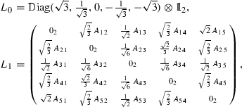
Let $(g,m)=(6,1)$ and $e_i\in D_i$ be unit vector fields. Furthermore, let $\overline{p}\in M_6$ and $p\in F_{\theta _j}^{-1}(\overline{p})$. Denote by $L_0$ and $L_1$ the shape operator of $M_6$ at $\overline{p}\in M_6$ with respect to $\nu _{\theta _6}(p)$ and $e_6(p)$, respectively. The isospectrality of $L(s)=\cos (s)L_0+\sin (s)L_1$ is equivalent to the classical Weyl identity with $(i,j)=(3,6)$ and the first four covariant derivatives with respect to $e_6\in D_6$ thereof.

Proof

We only give a sketch of the proof. First, we verify $L_0=\text{ Diag }(\sqrt{3},\frac{1}{\sqrt{3}},0,-\frac{1}{\sqrt{3}},-\sqrt{3})$ and

$$\begin{aligned} L_1=\left( \begin{array}{c@{\quad }c@{\quad }c@{\quad }c@{\quad }c} 0&{}\sqrt{\frac{2}{3}}\,\alpha _{1\,2\,6}&{}\frac{1}{\sqrt{2}}\,\alpha _{1\,3\,6}&{}\sqrt{\frac{2}{3}}\,\alpha _{1\,4\,6}&{}\sqrt{2}\,\alpha _{1\,5\,6}\\ \sqrt{\frac{2}{3}}\,\alpha _{1\,2\,6}&{}0&{}\frac{1}{\sqrt{6}}\,\alpha _{2\,3\,6}&{}\frac{\sqrt{2}}{3}\,\alpha _{2\,4\,6}&{}\sqrt{\frac{2}{3}}\,\alpha _{2\,5\,6}\\ \frac{1}{\sqrt{2}}\,\alpha _{1\,3\,6}&{}\frac{1}{\sqrt{6}}\,\alpha _{2\,3\,6}&{}0&{}\frac{1}{\sqrt{6}}\,\alpha _{3\,4\,6}&{}\frac{1}{\sqrt{2}}\,\alpha _{3\,5\,6}\\ \sqrt{\frac{2}{3}}\,\alpha _{1\,4\,6}&{}\frac{\sqrt{2}}{3}\,\alpha _{2\,4\,6}&{}\frac{1}{\sqrt{6}}\,\alpha _{3\,4\,6}&{}0&{}\sqrt{\frac{2}{3}}\,\alpha _{4\,5\,6}\\ \sqrt{2}\,\alpha _{1\,5\,6}&{}\sqrt{\frac{2}{3}}\,\alpha _{2\,5\,6}&{}\frac{1}{\sqrt{2}}\,\alpha _{3\,5\,6}&{}\sqrt{\frac{2}{3}}\,\alpha _{4\,5\,6}&{}0 \end{array}\right) , \end{aligned}$$

(6)

where $\alpha _{i\,j\,k}=\alpha _{|p}(e_i,e_j,e_k)$ for a $p\in F_{\theta _j}^{-1}(\overline{p})$. Substitute these results into the minimal polynomial equation for L(s). A tedious but straightforward calculation shows that the ideal generated by the resulting equations coincides with the ideal generated by the classical Weyl identity with $(i,j)=(3,6)$ and the first four covariant derivatives with respect to $e_6\in D_6$ thereof. $\square$

Advantages of the invariant Weyl identity. We shall now describe the advantages of the invariant Weyl identity deduced in the previous paragraph compared to the classical Weyl identities.

The discussion above, in particular Theorem 3.10, highlights what important role the higher covariant derivatives of the Weyl identities play in the classification. Since the classical Weyl identities depend on several indices, i.e., i and j, taking higher covariant derivatives of these identities would lead to a plethora of different cases. By contrast, in terms of the invariants $\hat{g}$, $\alpha$, and $B\otimes B^{-1}$ it is entirely possible to consider higher covariant derivatives since the Weyl identities are condensed in a single tensor identity.

In order to prove homogeneity of isoparametric hypersurfaces with $g=6$, one needs to analyze the interaction of the isospectral families that show up at different focal submanifolds (on the same normal great circle of $M^n$)—see also Sect. 4.1 for more details. The invariant Weyl identity contains all the information of isospectral families at different focal submanifolds!

For $g=3$ the Weyl identities turn each curvature distribution $D_j$ into a normed algebra [12]. An interesting question is if, as for $g=3$, there exists a geometric structure for $g=6$ captured by the Weyl identities. The existing examples suggest a geometry closely related to $\mathrm {G}_2$. This approach might lead to a viable strategy for completing classification.

Another open question is whether for $g=4$ the Weyl identity reflects parts of the Clifford algebra structure, which is the central underlying structure in this case.

4.3 Symmetry identities

Throughout this section p shall denote a fixed point of the manifold M.

Let $t\in {\mathbb {R}}$ and $k\in \mathbb {N}$ be given. The parallel surface map given by

$$\begin{aligned} F_t(p)\mapsto F_{t+2(\theta _k-t)}(p)=F_{2\theta _k-t}(p) \end{aligned}$$

maps the submanifold $F_t(M)\subset \mathbb {S}^{n+1}$ onto itself and flips the sign of $\nu _t$. Hence, there exist diffeomorphisms $\tau _k:M\rightarrow M$ such that

$$\begin{aligned} F_t{\circ \tau }_k=F_{2\theta _k-t} \quad \text{ and }\quad \nu _{t\vert \tau _k(p)}=-\nu _{2\theta _k-t|p}\quad \forall p\in M. \end{aligned}$$

Clearly, the maps $\tau _k:M\rightarrow M$ are reflections in the focal submanifolds, and in particular involutions.

Lemma 3.11

For $j\in \left\{ 1,\ldots ,g\right\}$, the map $\tau _j:M\rightarrow M$ is an isometry of $(M,{\hat{g}})$. Furthermore, the differences $\theta _j-\theta _k$ generate a discrete cyclic subgroup in ${\mathbb {R}}/{\mathbb {Z}\pi }$ and the involutions $\tau _j, 1\le j\le g$, are the reflections in the dihedral group $D_g=\left\langle \tau _1,\tau _g\right\rangle \subset \text{ Diff }(M)$.

Proof

The very definition of $\tau _k$ immediately implies $e^{-2i\theta _j}{\hat{F}}_0(p)={\hat{F}}_{2\theta _j}(p)=\overline{{\hat{F}}_0(\tau _j(p))}.$ Consequently, $e^{-2i\theta _j}d{\hat{F}}_{0\vert p}Y=\overline{d{\hat{F}}_{0\vert \tau _j(p)}d\tau _{j\vert p}Y}.$ Thus, we get

$$\begin{aligned} {\hat{g}}_{\vert p}(X,Y)={\hat{g}}_{\vert \tau _j(p)}(d\tau _{j\vert p}X,d\tau _{j\vert p}Y). \end{aligned}$$

$\square$

In the next theorem we prove the identities which we call symmetry identities.

Theorem 3.12

For $j\in \left\{ 1,\ldots ,g\right\}$ and $p\in M$

$$\begin{aligned} \alpha _{\vert p}(X,Y,Z)=-\alpha _{\vert \tau _j(p)}(d\tau _{j\vert p}X,d\tau _{j\vert p}Y,d\tau _{j\vert p}Z), \end{aligned}$$

or, for short, $(\tau _j)_*\alpha = -\alpha$. Furthermore, the higher covariant derivatives of $\alpha$ transform exactly as $\alpha$ does under $\tau _j$, i.e., $\nabla ^i\alpha =-(\tau _j)_{*}\nabla ^i\alpha$ for all $i\ge 0.$

Proof

By Theorem 2.14 and $F_0{\circ \tau }_j=F_{2\theta _j}$ we have

$$\begin{aligned} \alpha _{\vert p}(X,Y,Z)&=\alpha ^{2\theta _j}_{\vert p}(X,Y,Z) \\&=\left\langle dF_{0\vert \tau _j(p)}d\tau _{j\vert p}X,dF_{0\vert \tau _j(p)}d\tau _{j\vert p} \left( \nabla _{Y}^{2\theta _j}A_{2\theta _j}\right) Z\right\rangle _{\mathbb {S}^{n+1}}\\&= g_{0\vert \tau _j(p)}\left( d\tau _{j\vert p}X,d\tau _{j\vert p}\left( \nabla _{Y}^{2\theta _j}A_{2\theta _j}\right) Z\right) . \end{aligned}$$

The identities $F_0{\circ \tau }_j=F_{2\theta _j}$ and $\nu _0{\circ \tau }_j=-\nu _{2\theta _j}$ imply

$$\begin{aligned} A_{0\vert \tau _j(p)}d\tau _{j\vert p}X_1=-d\tau _{j\vert p}A_{2\theta _j\vert p}X_1 \end{aligned}$$

for all $p\in M$ and for all $X_1\in T_pM$. Moreover, the first identity also implies that $\tau _j:(M, g_{2\theta _j})\rightarrow (M, g_0)$ is an isometry. Thus, we get

$$\begin{aligned}&g_{0\vert \tau _j(p)}\left( d\tau _{j\vert p}X,d\tau _{j\vert p}\left( \nabla _{Y}^{\theta _j}\left( A_{2\theta _j}Z\right) -A_{2\theta _j}\nabla ^{2\theta _j}_{Y}Z\right) \right) \\ {}&= -g_{0\vert \tau _j(p)}\left( d\tau _{j\vert p}X,\left( \nabla _{d\tau _{j\vert p}Y}^{0}\left( A_{0}d\tau _{j\vert p}Z\right) -A_{0}\nabla ^{0}_{d\tau _{j\vert p}Y} d\tau _{j\vert p}Z\right) \right) \\ {}&=-\alpha _{\vert \tau _j(p)}\left( d\tau _{j\vert p}X,d\tau _{j\vert p}Y,d\tau _{j\vert p}Z\right) , \end{aligned}$$

and thus the first claim. From this the second claim is immediate. $\square$

Remark 3.13

• (1) Note that the symmetry identities relate $\alpha _p$ to $\alpha _q$, where p and q are different points of M. This means that in contrast to the Weyl identities, the symmetry identities are not pointwise identities.

• (2) In Section  4, Lemma 4.1 in [17] Miyaoka states some identities, which she refers to as ‘global symmetry’, and which were deduced by her in [13]. These identities are presumably equivalent to the symmetry identities. However, the author does not understand the proof of the ‘global identities’ in [13].

5 A geometric interpretation of homogeneity

In this section we prove that homogeneity of isoparametric hypersurfaces with $g=6$ is equivalent to a geometric property of the Lagrangian submanifold in the complex quadric. We hope that a detailed study of the geometry of the Lagrangian submanifold finally will lead to a geometric classification of isoparametric hypersurfaces in spheres with $g=6$.

This section is structured as follows: In the first subsection we recall what is known for the case $g=6$; in the second subsection we determine $\alpha$ for the homogeneous examples with $g=6$. Finally, in the third subsection, we give several equivalent formulations of homogeneity of isoparametric hypersurfaces with $g=6$.

5.1 Isoparametric hypersurfaces with $g=6$

In this subsection we summarize the known results for isoparametric hypersurfaces in spheres with $g=6$.

For the case of isoparametric hypersurfaces in spheres with $g=6$, all multiplicities coincide and are given either by $m=1$ or by $m=2$ [1]. Furthermore, exactly two examples with $g=6$ are known, both of which are homogeneous. They are given as orbits of the isotropy representation of $\mathrm {G}_2/\mathrm {SO}(4)$ or as orbits in the unit sphere $\mathbb {S}^{13}$ of the Lie algebra $\mathfrak {g}_2$ of the adjoint representation of the Lie group $\mathrm {G}_2$ and have multiplicities $m=1$ and $m=2$, respectively. The following conjecture is due to Dorfmeister and Neher and is believed to be true.

Conjecture

([9]) Each maximal isoparametric hypersurface with $g=6$ principal curvatures is homogeneous.

Dorfmeister and Neher proved this conjecture in the affirmative for the case $m=1$. Since homogeneous isoparametric hypersurfaces in spheres were classified by Takagi and Takahashi [30], this provides a classification of isoparametric hypersurfaces with $(g,m)=(6,1)$. Similarly, proving that isoparametric hypersurfaces with $(g,m)=(6,2)$ are homogeneous would yield a classification of such hypersurfaces. Note that the case $m=2$ is not classified yet, see the appendix of this paper. Therefore, proving the above conjecture still remains the goal for isoparametric hypersurfaces with $(g,m)=(6,2)$.

Below we explain the approach by Dorfmeister and Neher for the case $m=1$. The starting point of their work is the following algebraic description of isoparametric hypersurfaces in spheres which is due to Münzner.

Theorem 4.1

([20])

• (a) Let $M\subset \mathbb {S}^{n+1}$ be an isoparametric hypersurface with g distinct eigenvalues. Then there exists a homogeneous polynomial $F:{\mathbb {R}}^{n+2}\rightarrow {\mathbb {R}}$ of degree g and positive integers $m_1$ and $m_2$ such that M is an open submanifold of a level surface

  $$\begin{aligned} M_t=\mathbb {S}^{n+1}\cap F^{-1}(t) \end{aligned}$$

     for a $t\in (-1,1)$, and the identities

  $$\begin{aligned}&\langle \text{ grad }F(x),\text{ grad }F(x)\rangle =g^2\langle x,x\rangle ^{g-1},\\&\Delta F(x)=\tfrac{1}{2}(m_2-m_1)g^2\langle x,x\rangle ^{g/2-1} \end{aligned}$$

  and $n=\tfrac{g}{2}(m_1+m_2)$ are satisfied.

• (b) Conversely, for each homogeneous polynomial F of degree g satisfying the three identities in a), the level surfaces $M_t$, $t\in (-1,1)$, are isoparametric.

For the case of isoparametric hypersurfaces with $(g,m)=(6,1)$, Dorfmeister and Neher proved that there exists—up to isomorphism—only one isoparametric polynomial in ${\mathbb {R}}^8$. The central step in their proof is a partial classification of the so-called E-families. Dorfmeister and Neher provided homogeneity by showing that only one of the explicit examples of E-families is associated with an isoparametric hypersurface in a sphere.

In [27] the author gave a simplified proof of the theorem of Dorfmeister and Neher. The central step in [27] consists in classifying the isospectral families at one focal submanifold, which can be shown to be equivalent to classifying the E-families introduced in [9]. Below we reformulate the essential insights from [9] and [27] in terms of the isospectral families, since we use this notation throughout this paper.

The homogeneity of isoparametric hypersurfaces with $g=6$ is equivalent to the property that the kernels of the isospectral families L(s) are independent of s [9, 17]. Although requiring the family L(s) have eigenvalues $\pm \sqrt{3}, \pm 1/\sqrt{3}$, and 0, all with the same multiplicity m, is a very restrictive condition on the symmetric real $5m\times 5m$-matrices $A_{\nu _1}$ and $A_{\nu _2}$, so far no one has yet succeeded in classifying such matrices for $m\ge 2$. Examples of such matrices are provided by the irreducible representations of $\mathrm {SU}(2)$. Among these examples one finds cases where the kernel of L(s) is not constant when varying s. To prove homogeneity of isoparametric hypersurfaces with $g=6$, it thus does not suffice to study the properties of just one isospectral family. One also needs to analyze the interaction of the isospectral families that show up at different focal submanifolds (on the same normal great circle of M).

Miyaoka also worked on the classification of isoparametric hypersurfaces with $g=6$.

Her work on the case $(g,m)=(6,1)$ is contained in [15] and the corresponding erratum [18]. However, there is still a crucial gap in the erratum [18]—see [27] for details.

Miyaoka’s work on the case $(g,m)=(6,2)$ is contained in [17] and the corresponding erratum [19]. However, there is also a crucial gap in the erratum [19]—see Appendix of the present paper.

5.2 Calculation of $\alpha$ for the homogeneous examples with $g=6$

In the case $g = 6$ only two examples are known, both of which are homogeneous. They are given as orbits of the isotropy representation of $\mathrm {G}_2/\mathrm {SO}(4)$ or the compact real Lie group $\mathrm {G}_2$, respectively. In both cases all six principal curvatures coincide and are given by $m=1$ and $m=2$, respectively.

For both of the homogeneous examples Miyaoka [14, 16] calculated the Christoffel symbols

$$\begin{aligned} \Lambda _{i,j}^k:=g_{0}\left( \nabla ^0_{f_i}f_j,f_k\right) , \end{aligned}$$

where $(f_n)_{n=1}^{6m}$ is a $g_0$-orthonormal frame with $f_{i+6k}\in D_{i}$ for $i\in \{1,\cdots , 6\}$ and $k=0,\cdots ,m-1$. In what follows we use these results to determine $\alpha$ for the homogeneous examples.

From $A_0f_i=\lambda _{i}(0)f_i$ we obtain

$$\begin{aligned} (\nabla ^0_{X}A_0)f_i=(\lambda _{i}(0)-A_0)\nabla ^0_{X}f_i, \end{aligned}$$

where $X\in \Gamma (TM)$ and the index i in $\lambda _i(0)$ is interpreted to be cyclic of order 6. Thus, for $j\ne k$ we get

$$\begin{aligned} \Lambda _{i,j}^k=(\lambda _{j}(0)-\lambda _{k}(0))^{-1}\alpha (f_i,f_j,f_k). \end{aligned}$$

Instead of calculating $\alpha (f_i,f_j,f_k)$ we determine $\alpha (e_i,e_j,e_k)$, where $(e_i)_{i=1}^{6m}$ denotes the ${\hat{g}}$-orthonormal basis with $e_i\in D_{i}$, which is associated with the $g_0$-orthonormal basis $(f_i)_{i=1}^{6m}$. In other words,

$$\begin{aligned} e_i=\sqrt{2(1+(\lambda _{i}(0))^2)^{-1}}f_i, \end{aligned}$$

for $i\in \left\{ 1,\ldots ,6m\right\}$.

Substituting the Christoffel symbols [14] into the above equation we obtain the following lemma.

Lemma 4.2

For the homogeneous isoparametric hypersurfaces with $(g,m)=(6,1)$ the components $\alpha _{i\,j\,k}:=\alpha (e_i,e_j,e_k)$ are given by

$$\begin{aligned} \alpha _{1\,2\,3}=\alpha _{3\,4\,5}=\alpha _{1\,5\,6}=\sqrt{\tfrac{3}{2}},\,\alpha _{2\,4\,6}=-\sqrt{\tfrac{3}{2}},\,\alpha _{1\,3\,5}=-2\sqrt{\tfrac{3}{2}}. \end{aligned}$$

All other $\alpha _{i\,j\,k}$ with $i\le j\le k$ vanish.

Next we consider the case $(g,m)=(6,2).$ Following Miyaoka, we use the notation $\overline{f}_i:=f_{6+i},i\in \left\{ 1,\ldots ,6\right\}$. Furthermore, an entry $\overline{e}_i$ of $\alpha$ will be denoted by an index $\overline{i}$, e.g., $\alpha (\overline{e}_1,e_5,e_6)$ is denoted by $\alpha _{\overline{1}\,5\,6}.$ Clearly, $f_i$ and $\overline{f}_i$ constitute an orthonormal basis of the two-dimensional distribution $D_i$.

Remark 4.3

Note, that the above choice of $f_i$ and $\overline{f}_i$ is not canonical. This freedom in the choice of the basis is one of the reasons why computer computations, which aim to determine the possible $\alpha$, fail until today.

Substituting the Christoffel symbols [16] into the above equation we obtain the following lemma.

Lemma 4.4

For the homogeneous isoparametric hypersurfaces with $(g,m)=(6,2)$ the components $\alpha _{i\,j\,k}:=\alpha (e_i,e_j,e_k)$ are given by

$$\begin{aligned}&\alpha _{1\,\overline{5}\,6}=-\sqrt{\tfrac{3}{2}},\,\,\alpha _{\overline{1}\,5\,6}=\alpha _{1\,5\,\overline{6}}=\alpha _{\overline{1}\,\overline{5}\,\overline{6}}=\sqrt{\tfrac{3}{2}},\,\,\,\alpha _{2\,\overline{4}\,6}=-\sqrt{\tfrac{3}{2}},\,\,\alpha _{\overline{2}\,4\,6}=\alpha _{2\,4\,\overline{6}}=\alpha _{\overline{2}\,\overline{4}\,\overline{6}}=\sqrt{\tfrac{3}{2}},\\&\alpha _{1\,\overline{2}\,3}=-\sqrt{\tfrac{3}{2}},\,\,\alpha _{\overline{1}\,2\,3}=\alpha _{1\,2\,\overline{3}}=\alpha _{\overline{1}\,\overline{2}\,\overline{3}}=\sqrt{\tfrac{3}{2}},\,\,\,\alpha _{3\,\overline{4}\,5}=\sqrt{\tfrac{3}{2}},\,\,\alpha _{\overline{3}\,4\,5}=\alpha _{3\,4\,\overline{5}}=\alpha _{\overline{3}\,\overline{4}\,\overline{5}}=-\sqrt{\tfrac{3}{2}},\\&\alpha _{1\,\overline{3}\,5}=2\sqrt{\tfrac{3}{2}},\,\,\alpha _{\overline{1}\,3\,5}=\alpha _{1\,3\,\overline{5}}=\alpha _{\overline{1},\overline{3},\overline{5}}=-2\sqrt{\tfrac{3}{2}}. \end{aligned}$$

All other $\alpha _{i\,j\,k}$ with $i\le j\le k$ vanish.

We used the above results to guess equivalent formulations for homogeneity. The following subsection contains our results of this procedure.

5.3 Equivalent formulations of homogeneity

In this subsection we provide several equivalent formulations of homogeneity. Throughout this subsection let $X,Y,Z\in \Gamma (TM)$ and $i\in \left\{ 1,2,3\right\}$.

For proving an extended version of Theorem B we need two preparatory lemmas.

Lemma 4.5

Let $g=6$. For each $i\in \left\{ 1,\ldots ,6\right\}$ the identity

$$\begin{aligned} R\left( \pi _iX,\pi _{i+3}Y,\pi _{i+3}Y,\pi _iX\right) =\tfrac{1}{4}{{\mathrm{trace}}}_{{\hat{g}}}\left( \alpha (\pi _iX,\pi _{i+3}Y,\,\cdot \,)^2\right) \end{aligned}$$

holds, the index of the projections is interpreted to be cyclic of order 6.

Proof

An easy calculation yields , and thus, the claim follows from Proposition 3.1. $\square$

Lemma 4.6

Let $j\in \left\{ 1,\ldots ,6\right\}$. For each vector field $Z\in \Gamma (TM)$ introduce the vector field $\hat{Z}:=\pi _{{D_j\oplus D_{j+3}}}Z$. The direct sum $D_j\oplus D_{j+3}$ is integrable if and only if

$$\begin{aligned} \left( \nabla _{\hat{X}}B_{\theta _j}^2\right) {\hat{Y}} -\left( \nabla _{{\hat{Y}}}B_{\theta _j}^2\right) \hat{X}=0 \end{aligned}$$

(7)

holds for all $X,Y\in \Gamma (TM).$

Proof

By Sect. 2.4 we obtain

for $j\in \left\{ 1,\ldots ,6\right\}$. Hence, using we get the identity and thus

By interchanging the roles of X and Y and subtracting the resulting equation from the preceding equation we obtain

By definition of $B_t$ we get if and only if $Z\in D_j\oplus D_{j+3}$. Combining this with the previous identity yields the desired result. $\square$

In the next theorem we finally provide several equivalent formulations for homogeneity of isoparametric hypersurfaces in spheres with $g=6$.

Theorem 4.7

Each of the following statements is equivalent to the homogeneity of isoparametric hypersurfaces in spheres with $g=6$.

• (i) For each $i\in \left\{ 1,\ldots ,6\right\}$ we have

  $$\begin{aligned} \alpha (\pi _iX,\pi _{i+3}Y,Z)=0. \end{aligned}$$

• (ii) For $i,j,k\in \lbrace 1,\ldots ,6\rbrace$ with $j+k+l\not \equiv 0\,\,\text{ modulo }\,\,3$ we have

  $$\begin{aligned} \alpha (\pi _jX,\pi _{k}Y,\pi _{l}Z)=0. \end{aligned}$$

• (iii) The following identity is satisfied

  $$\begin{aligned} \sum _{j=0}^5{(-1)^j\alpha (B^jX,B^{-j}Y,Z)}=0. \end{aligned}$$

• (iv) The following sectional curvatures of $(M,{\hat{g}})$ vanish:

  $$\begin{aligned} R(\pi _iX,\pi _{i+3}Y,\pi _{i+3}Y,\pi _iX),\,i\in \left\{ 1,\ldots ,6\right\} . \end{aligned}$$

• (v) For $j\in \left\{ 1,\ldots ,6\right\}$ the direct sum $D_j\oplus D_{j+3}$ is integrable.

• (vi) The kernel of each linear isospectral family L(s) is independent of $s\in {\mathbb {R}}$.

Proof

It is well known that the sixth statement is equivalent to the homogeneity of isoparametric hypersurfaces in spheres with $g=6$ [9, 17]. Hence, it is sufficient to prove that the six statements are equivalent to each other.

• $(i)\Rightarrow (ii)$. Lemma 2.13 implies that $\alpha (\pi _jX,\pi _{k}Y,\pi _{l}Z)\ne 0$ can only hold if $(j,k,l)=(n,n+2,n+4)$ or $(j,k,l)=(n,n+1,n+2)$, up to a permutation of $n\in \{1,\ldots ,6\}$. Since in these cases the equation $i+j+k=0$ holds modulo 3, the claim is proved.

• $(ii)\Rightarrow (i)$. Choose $j=i$ and $k=i+3$ for some $i\in \left\{ 1,\ldots ,6\right\} .$ Then

  $$\begin{aligned} \alpha (\pi _iX,\pi _{i+3}Y,\pi _{l}Z)=0 \end{aligned}$$

  unless $l\in \left\{ i,i+3\right\}$. For $l\in \left\{ i,i+3\right\}$ the vanishing follows from Lemma 2.13.

• $(i)\Rightarrow (iii)$. Using Lemma 2.19 we get

  $$\begin{aligned} \sum _{\ell =1}^6{\pi _{\ell }\otimes \pi _{\ell +3}}=\tfrac{1}{6^2}\sum _{\ell =0}^5{\sum _{k,j=0}^5{B_{\theta _{\ell }}^k\otimes B_{\theta _{\ell +3}}^j}}=\tfrac{1}{6^2}\sum _{\ell =0}^5{\sum _{k,j=0}^5{(-1)^jB_{\theta _{\ell }}^k\otimes B_{\theta _{\ell }}^j}}, \end{aligned}$$

  where we made use of the last identity of Lemma 2.17 and $\theta _{\ell +3}=\theta _{\ell }+\frac{\pi }{2}$ to obtain the last equality. By Lemma 2.17 again we obtain

  $$\begin{aligned} \tfrac{1}{6^2}\sum _{\ell =0}^5{\sum _{k,j=0}^5{(-1)^jB_{\theta _{\ell }}^k\otimes B_{\theta _{\ell }}^j}}= \tfrac{1}{6^2}\sum _{\ell =0}^5{\sum _{k,j=0}^5{(-1)^j\xi ^{(j+k)\ell }B_{-\pi /12}^k \otimes B_{-\pi /12}^j}}, \end{aligned}$$

  where we introduced $\xi =e^{-i\frac{\pi }{3}}$. Thus, we get

  $$\begin{aligned} \tfrac{1}{6^2}\sum _{\ell =0}^5{\sum _{k,j=0}^5{(-1)^j\xi ^{(j+k)\ell } B_{-\pi /12}^k \otimes B_{-\pi /12}^j}}= \tfrac{1}{6}\sum _{j=0}^5{(-1)^jB_0^j \otimes B_0^{-j}}, \end{aligned}$$

  where we made use of Lemma 2.17 to get the last equality. Combined we get

  $$\begin{aligned} \sum _{\ell =1}^6{\pi _{\ell }\otimes \pi _{\ell +3}}=\tfrac{1}{6}\sum _{j=0}^5{(-1)^jB_0^j \otimes B_0^{-j}}. \end{aligned}$$

  Hence, (i) implies

  $$\begin{aligned} \tfrac{1}{6}\sum _{j=0}^5{(-1)^j\alpha (B_0^jX,B_0^{-j}Y,Z)}=\sum _{i=1}^6{\alpha (\pi _i^{t}X,\pi _{i+3}^{t}Y,Z)}=0. \end{aligned}$$

  (8)

• $(iii)\Rightarrow (i)$. Let $1\le k\le 6$ be given. Substitute $X=\pi _kX_1$ and $Y=\pi _{k+3}Y_1$, $X_1,Y_1\in \Gamma (TM)$, in Eq. (8) and use $\pi _i\circ \pi _j=\delta _{i,j}$ for any $i,j\in \lbrace 1,..,6\rbrace$.

• $(i)\Leftrightarrow (iv)$. One direction is immediate from Lemma 4.5 and the other follows from the fact that $\alpha$ is real.

• $(i)\Rightarrow (v)$. Eq. (7) is equivalent to the statement

  $$\begin{aligned} {\hat{g}}((\nabla _{\hat{X}}B_{\theta _j}^2){\hat{Y}}-(\nabla _{{\hat{Y}}}B_{\theta _j}^2)\hat{X},Z)=0 \end{aligned}$$

  for all $X,Y,Z\in \Gamma (TM)$. Making use of Lemma 3.6 and the equalities $B_{\theta _j}\pi _j X=\pi _j X$ and $B_{\theta _j}\pi _{j+3} X=-\pi _{j+3} X$ one finds that the preceding equation is equivalent to

  $$\begin{aligned} \alpha (\hat{X},B_{\theta _j}{\hat{Y}},B_{\theta _j}Z)-\alpha (B_{\theta _j}\hat{X},{\hat{Y}}, B_{\theta _j}Z)=0. \end{aligned}$$

  This equation is satisfied since

  

  holds by (ii) and Lemma 2.13.

• $(v)\Rightarrow (i)$. Making again use of the equations $B_{\theta _j}\pi _j X=\pi _j X$ and $B_{\theta _j}\pi _{j+3} X=-\pi _{j+3} X$ one verifies easily that Eq. (7) is equivalent to

  $$\begin{aligned} \alpha (\pi _jX,\pi _{j+3}Y,Z)-\alpha (\pi _{j+3}X,\pi _{j}Y,Z)=0\quad \text{ for } \text{ all }\quad Z\in \Gamma (TM). \end{aligned}$$

  Applying this equation to $X=\pi _jX_1$ and $Y=\pi _{j+3}Y_1$, for arbitrary $X_1,Y_1\in \Gamma (TM)$, yields the claim.

• $(vi)\Rightarrow (i)$. We first assume $m=1$. In the proof of Theorem 3.10, we described the linear isospectral family $L(s)=\cos (s)L_0+\sin (s)L_1$, $s\in {\mathbb {R}}$, of the focal submanifold $F_{\theta _6}$ for the case $m=1$ in terms of $\alpha _{i\,j\,\,k}$, see Eq. (6). Clearly, the kernel of $L_0$ is given by $e_3=(0,0,1,0,0)^{tr}$. Hence, the constancy of the kernel of L(s) implies that the kernel of $L_1$ is also given by $e_3$. By (6), this is equivalent to the identity $\alpha (\pi _3X,\pi _6Y,Z)=0$. Carrying out analogous considerations for $F_{\theta _j}, j\in \lbrace 1,\ldots ,5\rbrace$, we finally get $\alpha (\pi _iX,\pi _{i+3}Y,Z)=0$ for all $i\in \lbrace 1,\ldots ,6\rbrace$. The case $m=2$ is proved analogously. Indeed, consider again the linear isospectral family $L(s,t)=\cos (s)L_0+\sin (s)(\cos (t)L_1+\sin (t)L_2)$, $s,t\in {\mathbb {R}}$, of the focal submanifold $F_{\theta _6}$ in terms of $\alpha _{i\,j\,\,k}$. Here we have

  
  $$\begin{aligned} L_2=\left( {\begin{matrix} 0_2&{}\quad \sqrt{\frac{2}{3}}\,B_{1\,2}&{}\quad \frac{1}{\sqrt{2}}\,B_{1\,3}&{}\quad \sqrt{\frac{2}{3}}\,B_{1\,4}&{}\quad \sqrt{2}\,B_{1\,5}\\ \sqrt{\frac{2}{3}}\,B_{2\,1}&{}\quad 0_2&{}\quad \frac{1}{\sqrt{6}}\,B_{2\,3}&{}\quad \frac{\sqrt{2}}{3}\,B_{2\,4}&{}\quad \sqrt{\frac{2}{3}}\,B_{2\,5}\\ \frac{1}{\sqrt{2}}\,B_{3\,1}&{}\quad \frac{1}{\sqrt{6}}\,B_{3\,2}&{}\quad 0_2&{}\quad \frac{1}{\sqrt{6}}\,B_{3\,4}&{}\quad \frac{1}{\sqrt{2}}\,B_{3\,5}\\ \sqrt{\frac{2}{3}}\,B_{4\,1}&{}\quad \frac{\sqrt{2}}{3}\,B_{4\,2}&{}\quad \frac{1}{\sqrt{6}}\,B_{4\,3}&{}\quad 0_2&{}\quad \sqrt{\frac{2}{3}}\,B_{4\,5}\\ \sqrt{2}\,B_{5\,1}&{}\quad \sqrt{\frac{2}{3}}\,B_{5\,2}&{}\quad \frac{1}{\sqrt{2}}\,B_{5\,3}&{}\quad \sqrt{\frac{2}{3}}\,B_{5\,4}&{}\quad 0_2 \end{matrix}} \right) , \end{aligned}$$

  where

  $$\begin{aligned} A_{i\,j}=\left( \begin{array}{c@{\quad }c} \alpha _{i\,j\,6}&{}\alpha _{i\,\overline{j}\,6}\\ \alpha _{\overline{i}\,j\,6}&{}\alpha _{\overline{i}\,\overline{j}\,6}\\ \end{array}\right) \quad \text{ and }\quad B_{i\,j}=\left( \begin{array}{c@{\quad }c} \alpha _{i\,j\,\overline{6}}&{}\alpha _{i\,\overline{j}\,\overline{6}}\\ \alpha _{\overline{i}\,j\,\overline{6}}&{}\alpha _{\overline{i}\,\overline{j}\,\overline{6}}\\ \end{array}\right) . \end{aligned}$$

  As in the case $m=1$, the constancy of the kernel of L(s, t) implies the identity $\alpha (\pi _3X,\pi _6Y,Z)=0$. Again, the claim is established by carrying out analogous considerations for $F_{\theta _j}, j\in \lbrace 1,\ldots ,5\rbrace$.

• $(i)\Rightarrow (vi)$. Let us first consider the case $m=1$. Since $\alpha (\pi _iX,\pi _{i+3},Y,Z)=0$ for all $i\in \lbrace 1,\ldots ,6\rbrace$, all entries of the third row (and thus the third column) of L(s) are 0. Thus, $e_3$ (the third vector of the standard basis in ${\mathbb {R}}^5$) lays in the kernel of L(s) for all $s\in {\mathbb {R}}$. Since the kernel of L(s) is one-dimensional, the claim is established. Next, suppose $m=2$. Since $\alpha (\pi _iX,\pi _{i+3},Y,Z)=0$ for all $i\in \lbrace 1,\ldots ,6\rbrace$, all entries of the fifth and the sixth rows (and thus the fifth and the sixth columns) of L(s, t) are 0. Thus, $e_5$ and $e_6$ (the fifth and sixth vectors of the standard basis in ${\mathbb {R}}^{10}$) lay in the kernel of L(s, t) for all $s,t\in {\mathbb {R}}$. Since the kernel of L(s, t) is two-dimensional, the claim is established.

$\square$

Using the classification of isoparametric hypersurfaces in spheres with $g=6$ and $m=1$ given by Dorfmeister and Neher [9], we obtain the following corollary.

Corollary 4.8

Assume $(g,m)=(6,1).$ For all $i\in \left\{ 1,\ldots ,6\right\}$ the sectional curvatures $R(\pi _iX,\pi _{i+3}Y,\pi _{i+3}Y,\pi _iX)=0$ of $(M,{\hat{g}})$ vanish.

Theorem 4.7 establishes a new strategy for proving homogeneity of isoparametric surfaces in spheres with $g=6$: We hope that a detailed study of the geometry of the Lagrangian submanifold in the complex quadric might be helpful.

Appendix: A counterexample to Miyaoka’s proof in [17, 19]

Let $\overline{p}$ be a point of a fixed focal submanifold $M_+$. Without loss of generality we assume $M_+=M_6$. Recall from Sect. 3.2.3 that $T_{\overline{p}}M_6=\oplus _{i=1}^5D_i(p)$, where $p\in F_{\theta _j}^{-1}(\overline{p})$, and that the normal space $\nu _{\overline{p}}M_6$ of $M_6$ at $\overline{p}$ is spanned by $\nu _{\theta _6}(p)$ and a basis of $D_j(p)$.

We follow the notation of Miyaoka and let $\eta _p=\nu _{\theta _6}(p)$ and $\xi _p\in D_6(p)$. In Miyaoka [17] introduced

$$\begin{aligned} E(c)=E(p,\xi _p)=\text{ span }\{\text{ Ker }L(t)\,|\,t\in [0,2\pi )\}, \end{aligned}$$

where $c(t)=\cos (t)\eta _p+\sin (t)\xi _p$ and $L(t)=\cos (t)A_{\eta _p}+\sin (t)A_{\xi _p}$ is an isospectral family of focal shape operators.

In [19] Miyaoka introduced

$$\begin{aligned} E=\text{ span }\{ E(c)\,|\,\text{ c } \text{ geodesic } \text{ of }\,L_6(p)\}, \end{aligned}$$

where $L_6(p)$ denotes the leaf of $D_6$ through p. Since $m=2$, the unit vector $\xi _p$ is of the form $\xi _p=\cos (s)e_6(p)+\sin (s)e_{\overline{6}}$, where the vectors $e_6(p),e_{\overline{6}}(p)$ constitute an orthonormal basis of $D_6(p)$. Consequently, we have

$$\begin{aligned} E=\text{ span }_{t,s}\text{ Ker }L(t,s), \end{aligned}$$

where L(t, s) is given by

$$\begin{aligned} L(t,s)=&\cos (t)A_{\eta _p}+\sin (t)A_{\cos (s)e_6(p)+\sin (s)e_{\overline{6}}(p)}\\=&\cos (t)A_{\eta _p}+\sin (t)(\cos (s)A_{e_6(p)}+\sin (s)A_{e_{\overline{6}}(p)}). \end{aligned}$$

In Proposition 6.2 on page 8 in the erratum [19], Miyaoka claims that if $\dim E(c)=4$, then all the shape operators L(t, s) map E onto $E^{\perp }$. This statement is not correct, which is shown by the following counterexample.

Counterexample

We give an example of an isoparametric family L(t, s) such that $\dim E(c)=4$ and $\dim E>4$ but L(t, s) does not map E to $E^{\perp }$.

We use the short-hand notation $A_{\eta _p}=L_0$, $A_{e_6(p)}=L_1$ and $A_{e_{\overline{6}}(p)})=L_2$. Furthermore, let

$$\begin{aligned} L_0=\text{ diag }(\sqrt{3},\sqrt{3},1/\sqrt{3},1/\sqrt{3},0,0,-1/\sqrt{3},-1/\sqrt{3},-\sqrt{3},-\sqrt{3}), \end{aligned}$$

$$\begin{aligned}&L_2=\tfrac{1}{\sqrt{6}}\left( {\begin{matrix} 0_2&{}\quad 0_2&{}\quad 0_2&{}\quad 0_2&{}\quad -3\sqrt{2}J\\ 0_2&{}\quad 0_2&{}\quad -J&{}\quad 0_2&{}\quad 0_2\\ 0_2&{}\quad J&{}\quad 0_2&{}\quad -J&{}\quad 0_2\\ 0_2&{}\quad 0_2&{}\quad J&{}\quad 0_2&{}\quad 0_2\\ 3\sqrt{2}J&{}\quad 0_2&{}\quad 0_2&{}\quad 0_2&{}\quad 0_2 \end{matrix}} \right) \end{aligned}$$

where $J=\left( {\begin{matrix} 0&{}\quad -1\\ 1&{}\quad 0 \end{matrix}} \right)$. One verifies easily that $L(t,s)=\cos (t)L_0+\sin (t)(\cos (s)L_1+\sin (s)L_2)$ is isospectral, i.e., the spectrum is given by $\text{ spec }(L(t,s))=\{\sqrt{3},1/\sqrt{3},0,-1/\sqrt{3},-\sqrt{3}\}$, where each eigenvalue occurs with multiplicity 2.

One verifies easily that for given $s\in {\mathbb {R}}$, i.e., a fixed geodesic c in $L_6(p)$, the vectors

$$\begin{aligned}&(0, 0, -\sin (2s), -\cos (2s), 0, 0, 0, 1, 0, 0)^{tr}, \\&(0, 0, 0, 0, \sin (s),\cos (s), 0, 0, 0, 0)^{tr}, \\&(0, 0, 0, 0, \cos (s), -\sin (s), 0, 0, 0, 0)^{tr},\\&(0, 0, -\cos (2s), \sin (2s), 0, 0, 1, 0, 0, 0)^{tr} \end{aligned}$$

constitute a basis of E(c). Hence, we have $\dim E(c)=4$.

From this we get $E=\text{ span }\{e_3,e_4,e_5,e_6,e_7,e_8\}$, where $e_i$ denotes the ith unit vector in ${\mathbb {R}}^{10}$. Furthermore, we obtain $L(t,s)E \not \subset E^{\perp }$. Note that even $L_0E\not \subset E^{\perp }$.

The preceding counterexample clearly shows that we cannot deduce the identity $L_0E=E^{\perp }$ as long as we just deal with the linear isospectral family at one fixed focal submanifold. In order to generate such an identity (which would hold if isoparametric hypersurfaces with $g=6$ and $m=2$ are indeed homogeneous) one has to analyze the interaction of the isospectral families at different focal submanifolds.

Remark 4.9

In the proof of Proposition 6.2 in [19], Miyaoka considers the linear isospectral family at one fixed focal submanifold. Furthermore, she brings the ‘global symmetry’ into play. However, she uses this identity only to prove that a certain subspace $W\subset T_{\overline{p}}M_6\cong {\mathbb {R}}^{10}$ actually coincides with the orthogonal complement $E^{\perp }$ of E and not to show $L_0E=E^{\perp }$.

Finding a successful way to analyze the interaction of the isospectral families at different focal submanifolds is one of the central problems that have to be solved in order to classify isoparametric hypersurfaces in spheres with $g=6$ and $m=2$.

References

Abresch, U.: Isoparametric hypersurfaces with four or six distinct principal curvatures. Math. Ann. 264, 283–302 (1983)
Cartan, E.: Familles de surfaces isoparamétriques dans les espaces à courbure constante. Ann. Mat. Pura Appl. 17, 177–191 (1938)
Cartan, E.: Sur des familles remarquables d’hypersurfaces isoparamétriques dans les espaces sphériques. Math. Z. 45, 335–367 (1939)
Cartan, E.: Sur quelques familles remarquables d’hypersurfaces. C. R. Congrès Math. Liège. 1, 30–41 (1939)
Cartan, E.: Sur des familles d’hypersurfaces isoparamétriques des espaces sphériques à \(5\) et à \(9\) dimensions. Revista Univ. Nac. Tucumán, Revista A 1, 5–22 (1940)
Cecil, T.: Isoparametric and Dupin hypersurfaces. SIGMA 4, 197–211 (2008)
Cecil, T., Chi, Q., Jensen, G.: Isoparametric hypersurfaces with four principal curvatures. Ann. Math. 166, 1–76 (2007)
Chi, Q.: Isoparametric hypersurfaces with four principal curvatures, IV, arXiv:1605.00976
Dorfmeister, J., Neher, E.: Isoparametric hypersurfaces, case \(g=6\), \(m=1\). Comm. Algebra 13, 2299–2368 (1985)
Ferus, D., Karcher, H., Münzner, H.F.: Cliffordalgebren und neue isoparametrische Hyperflächen. Math. Z. 177, 479–502 (1981)
Gasqui, J., Goldschmidt, H.: Radon transforms and the rigidity of the Grassmannians. Annals of Mathematics Studies, p. 384. Princeton University Press, Princeton (2004)
Karcher, H.: A geometric classification of positively curved symmetric spaces and the isoparametric construction of the Cayley plane, Lecture Notes (Rome)
Miyaoka, R.: Dupin hypersurfaces with six principal curvatures. Kodai Math. J. 12, 308–315 (1989)
Miyaoka, R.: The linear isotropy group of \(G_2/ \text{ SO }(4)\), the Hopf fibering and isoparametric hypersurfaces. Osaka J. Math. 30, 179–202 (1993)
Miyaoka, R.: The Dorfmeister-Neher theorem on isoparametric hypersurfaces. Osaka J. Math. 46, 695–715 (2009)
Miyaoka, R.: Geometry of \(\text{ G }_{2}\) orbits and isoparametric hypersurfaces. Nagoya Math. J. 203, 175–189 (2011)
Miyaoka, R.: Isoparametric hypersurfaces with \((g, m)=(6,2)\). Ann. Math. 177, 53–110 (2013)
Miyaoka, R.: Remarks on the Dorfmeister-Neher theorem on isoparametric hypersurfaces. Osaka J. Math. 52, 373–377 (2015)
Miyaoka, R.: Errata of ‘Isoparametric hypersurfaces with (g, m)=(6,2)’. Ann. Math. 183, 1057–1071 (2016)
Münzner, H.F.: Isoparametrische Hyperflächen in Sphären. Math. Ann. 251, 57–71 (1980)
Münzner, H.F.: Isoparametrische Hyperflächen in Sphären II. Math. Ann. 255, 215–232 (1981)
Ma, H., Ohnita, Y.: On Lagrangian submanifolds in complex hyperquadrics and isoparametric hypersurfaces in spheres. Math. Z. 261, 749–785 (2009)
Nomizu, K.: Some results in E. Cartan’s theory of isoparametric families of hypersurfaces. Bull. Am. Math. Soc. 79, 1184–1188 (1973)
Palmer, B.: Buckling eigenvalues, Gauss maps and Lagrangian submanifolds. Differ. Geom. Appl. 4, 391–403 (1994)
Palmer, B.: Hamiltonian minimality and Hamiltonian stability of Gauss maps. Differ. Geom. Appl. 7, 51–58 (1997)
Segre, B.: Famiglie di ipersuperficie isoparametriche negli spazi euclidei ad un qualunque numero di dimensioni. Atti. Accad. Naz. Lincei, Rend., VI. Ser. 27, 203–207 (1938)
Siffert, A.: Classification of isoparametric hypersurfaces in spheres with \((g, m)=(6,1)\). Proc. Am. Math. Soc. 144, 2217–2230 (2016)
Somigliana, C.: Sulle relazioni fra il principio di Huygens e l’ottica geometrica. Atti. Acc. Sci. Torino 54, 974–979 (1919)
Stolz, S.: Multiplicities of Dupin hypersurfaces. Invent. Math. 138, 253–279 (1999)
Takagi, R., Takahashi, T.: On the principal curvatures of homogeneous hypersurfaces in a sphere. Differential geometry (in honor of Kentaro Yano), pp. 469–481. Kinokuniya, Tokyo (1972)
Thorbergsson, G.: A survey on isoparametric hypersurfaces and their generalizations. Handb. Differ. Geom. I, 963–995 (2000)
Acknowledgements
Open access funding provided by Max Planck Society. It is a pleasure to thank Prof. Dr. Uwe Abresch for introducing me to isoparametric hypersurfaces and for his generous support. I benefitted enormously from numerous mathematical discussions with him. Furthermore, I am very grateful to Prof. Dr. Wolfgang Ziller and Prof. Dr. Gudlaugur Thorbergsson for their many valuable comments and for fruitful mathematical discussions. Moreover, I would like to thank the referee for carefully reading the manuscript and for giving such constructive comments which substantially helped to improve the quality of the manuscript. This work was finished while the author was supported by Deutsche Forschungsgemeinschaft with the Grant SI 2077/1-1. Last, but not least, I would like to thank the Max Planck Institute for Mathematics in Bonn for providing excellent working conditions.
Author information
Authors and Affiliations
Corresponding author
Additional information
This work was finished while the author was supported by DFG grant SI 2077/1-1.