
Abstract
Can prices convey information about the fundamental value of an asset? This paper considers this problem in relation to the dynamic properties of the fundamental (whether it is constant or time-varying) and the structure of information available to agents. Risk-averse traders receive two potential signals each period: one exogenous and private and the other, prices, endogenous and public. Prices aggregate private information but include aggregate noise. Information can accumulate over time both through endogenous and exogenous signals. With a constant fundamental, the precision of both private and public cumulative information increases over time but agents put progressively more weight on the endogenous signals, asymptotically disregarding private ones. If the fundamental is time-varying, the use of past private signals complicates the role of prices as a source of information, since it introduces endogenous serial correlation in the price signal and cross-correlation between it and innovations in the fundamental. A modified version of the Kalman filter can still be used to extract information from prices and results show that the precision of the endogenous signals converges to a constant, with both private and public information used at all times.
1 Introduction
The aim of this paper is to analyse the ability of prices to convey information about the fundamental value of an asset, in particular in relation to the nature of the fundamental, whether it is constant or time-varying. To this end, I consider a multi-period model with diffuse information, where agents receive sequential signals and use them optimally (in a Bayesian sense) to estimate the fundamental value of an asset. The nature of the fundamental and the structure of information available, which is endogenous in the case of prices, determine the optimal weights on private and public signals. The evolution of such weights over time is the central element of investigation of this paper.
To explore these issues, I employ a model where risk averse agents invest in a risky one-period asset: this means that all they need to know to make their investment decision is the current price and the liquidation value next period, equal to its fundamental value, while there is no need to forecast future prices. To allow for the accumulation of information over time, I adopt the modelling strategy proposed in Vives (1995b) and assume that in each period agents submit their market orders but trade takes place with some probability: if it does, the asset is liquidated at the end of the period and the market ends; if not, the following period the same process repeats, and agents can observe the equilibrium prices from previous periods. The purpose of this assumption is to isolate the analysis from issues related to expectations about future prices and higher order beliefs: in this setting, the only possible informational role of prices is to provide information about other agents’ beliefs about the fundamental value. The liquidation value, which represents the fundamental value of the asset, is unknown to agents and only indirectly inferable through signals. Specifically, each period a trader receives a noisy exogenous private signal about the fundamental value, which remains available at successive times if trade is not realized. Besides this exogenous signal, agents can also use prices in their inference, as prices summarize the view of other market participants and thus can in principle convey important information about the fundamental value. Bayesian theory provides the optimal weights on the available signals.
There are two main contributions in this work. The first is to show that, with a constant fundamental, even when information can accumulate through both exogenous private and endogenous public signals, asymptotically agents use only prices as a source of information. This result is not obvious, and it relies on the precision of the cumulative signal from prices to increase at a faster rate than that from exogenous information. It extends results from Vives (1995b), where it is shown that prices become asymptotically fully revealing when information can accumulate through prices only.
The second contribution of this paper is to show how agents can use prices as a source of information when the fundamental is time-varying. Endogenous correlation structures must be accounted for, through a modified Kalman filter. Results show that asymptotically agents use both signals, as the precision of both private and public information remains finite and converges to a constant. To the best of my knowledge, this is the first time the informational role of prices is considered in a framework with a time-varying fundamental.
The dynamic properties of the fundamental have a deep impact on the informational content of prices. If the fundamental is constant over time, it is optimal for agents to put increasing weight on the price signal as information accumulates, and in the limit the private exogenous signal is completely ignored: prices become fully revealing, even in the presence of aggregate noise. A version of the Grossman–Stiglitz paradox thus reappears when agents have the possibility to observe sequential signals on the constant fundamental value. The paradox, though, does not bite here, as prices converge to the fundamental value as agents progressively switch from private to public information. This result has been noted before, notably in Vives (1995b), and it relies on the precision of public information to increase without bounds: here though, contrary to Vives (1995b), also the precision of private information increases without limit, so it is not obvious that such result would persist. The reason why it does is that, because of risk averse agents, the precision of public information grows at a faster rate than that of private information, thus leading to an increasing Bayesian weight on price signals.
The precision of agents’ estimates grows without limit because they receive sequential signals on a constant fundamental: as the number of conditionally independent observations grows large, the law of large numbers implies that the variance of the estimates decreases to zero. The same cannot happen when the fundamental is changing over time, and issues arise on the ability of prices to aggregate private signals and convey information about the changing fundamental. To investigate if prices can still reveal information in this case, I assume the fundamental follows a random walk process. As prices aggregate current and past information used in the estimation of the fundamental, prices now include the whole history of innovations in the random walk, and thus show both serial correlation and cross correlation with the fundamental. The use of prices as signals becomes thus problematic as the endogenous and time-varying correlation structures need to be accounted for. I show how this can be done in the context of a Kalman filter, and what the implications are for the informativeness of prices. The endogenous correlations depend on the sequence of past Kalman gains, and in turn determine the current gain: this recursion leads to gains (and thus weights on the two signals) that converge to a constant. Moreover, while the length of the serial and cross correlations in the price signals increases with time, their conditional variance converges to a constant. In equilibrium thus agents receive two signals on the current value of the fundamental, one exogenous and one endogenous, both with constant and finite precision, which lead to a constant variance in the Kalman estimates.
1.1 Related literature
The problems of information aggregation through prices and of the informational efficiency of markets in the presence of heterogeneous information has been widely considered in the literature. In seminal works, Grossman (1976, (1978) show how prices can aggregate information perfectly and substitute for private information in markets. This result raises the possibility of an interesting paradox, as pointed out famously by Grossman and Stiglitz (1980): if prices aggregate private information perfectly, no trader would have any incentive to acquire such information, as they could simply look at prices, but then there would be no information for prices to aggregate. A common approach to get past this paradox is to include aggregate noise in prices, as in, for example, Hellwig (1980) and Diamond and Verrecchia (1981). The inclusion of aggregate noise solves the paradox, as prices are only partially revealing in equilibrium and thus agents have an incentive to acquire private information.
Another way to resolve the paradox is to consider markets with a finite number of traders who have market power, as for example in Kyle (1989) and Jackson (1991): market power ensures that prices only partially reveal private information, thus maintaining an incentive for agents to acquire such information. A further way out of the paradox, recently proposed by Vives (2014), is to distinguish between common and private value components in the valuations of traders, with signals only providing bundled information about these components.
All these works consider static settings, where information is only received once. Noisy rational expectations equilibria, though, have also been analyzed in dynamic settings. Vives (1993) studies the rate at which dispersed information is incorporated into prices with risk neutral firms. Convergence is slow with finite precision of private information but a positive mass of perfectly informed agents speeds up convergence.
Vives (1995b) studies the rate at which dispersed private information about the value of a risky asset is incorporated into prices with risk averse agents: the speed of information revelation is found to depend crucially on the presence of a competitive risk neutral market making sector.
Vives (1995a) considers instead the effect of investors’ horizons on the informational content of prices in a finite-horizon model with risk averse agents. The effect depends on the temporal pattern of private information arrival: long horizons reduce the final price informativeness when the arrival of information is diffuse (as in the present paper); nevertheless, as the number of trading periods increases without bound, prices converge to the fundamental value.
Kyle (1985) analyses how quickly new private information about the underlying value of a speculative commodity gets incorporated into market prices and how it affects the liquidity of the market. The model has three kinds of traders: a single risk neutral insider, random noise traders, and competitive risk neutral market makers. The insider makes positive profits by exploiting his monopoly power, with noise trading concealing his trading from market makers. In the limit, as the time interval between auctions goes to zero, all private information is incorporated into prices through trading.
Amador and Weill (2012) consider a dynamic framework where agents learn from the actions of others through two channels: a public channel, such as equilibrium market prices, and a private channel, such as local interactions: when agents learn only from the public channel, an initial release of public information increases knowledge and welfare, while if a private learning channel is also present, the result is reversed and an increase in initial public information reduces agents’ asymptotic knowledge. Importantly, while the initial signals realizations are centered around the true state of the world, subsequent realizations are centered around the endogenous actions of agents: that is, after the first period, all new information about the state of the world comes from others and there is no additional arrival of new exogenous information. This possibility is instead crucial for results I will present in this paper.
Differently from all these works, I do not focus on the speed of information revelation, the structure of the market, the informational type of traders or their investment horizon. The focus of the paper is instead on the relation between the dynamic properties of the fundamental, the structure of the endogenous signal and the informational content of prices.
An important issue that is not addressed in this paper is the role of higher order beliefs on prices under heterogeneous information and how they interact with sequential signals. To avoid dealing with the interaction between higher order beliefs and the accumulation of information on fundamentals, I limit the setting to a one-period asset, so that agents do not need to forecast future prices and only use prices as a signal for other agents’ beliefs about the fundamental. Seminal papers on the problem of higher order beliefs are Townsend (1983) and Sargent (1991), and more recent treatments are proposed in Allen, Morris and Shin (2006), Kasa et al. (2014) and Nimark (2017).
2 The model
I assume there is a risky one-period asset available for trade on the market. Traders submit their demand schedules based on the information they have and an auctioneer aggregates all orders and determines the equilibrium price. Trade then takes place with some given probability: if it does, then the asset is liquidated at the end of the period at the value \(\theta _{t}\) and the market ends; if not, the following period the same process repeats. The liquidation value \(\theta _{t}\) thus represents the fundamental value of the asset for traders.
The market is populated by a continuum of agents of unit mass, indexed by \( i\in [0,1]\), homogeneous in all aspects except for the private information they receive, which will be specified below. In deciding their demand of shares, agents are mean variance maximizers, so they maximize the expected return of their investment subject to a penalty for the variance.Footnote 1 The problem for a trader i at time t is thus to choose the number of shares ( \(s_{t}^{i}\)) such that
where \(\gamma \) is the coefficient of risk aversion and the return on the portfolio of agent i at time t, \(R_{t}^{i}\), is defined as the difference between its liquidation value and what one has to pay for itFootnote 2
The expectational operator \(E_{t}^{i}\) represents the conditional expectations of agent i at time t given their information set \({\mathcal {I}}_{t}^{i}\): \(E_{t}^{i}X=E\left[ X\mid {\mathcal {I}}_{t}^{i}\right] \).
It follows that the optimal demand for trader i is
where \(\sigma _{{\hat{\theta }}_{t}}^{2}\) is the conditional variance of the prediction error associated to \(E_{t}^{i}\theta _{t}\).Footnote 3
In order to close the model with an equilibrium condition, I assume that the supply of shares \(\varepsilon _{t}\) is an i.i.d. random variable following a Normal distribution with zero mean and variance \(\sigma _{\varepsilon }^{2}\) . An exogenous and stochastic supply is often interpreted in the literature as coming from noise traders. Other interpretations of this aggregate noise term refer to variations in the availability of publicly tradable shares (asset float), as in Branch and Evans (2011), or to some unspecified random supply, as in Mele and Sangiorgi (2015). Independently of its interpretation, this aggregate noise term can prevent prices from being fully revealing, a common result in the literature on noisy rational expectations equilibria. Indeed, adopting the same assumption, Allen, Morris and Shin (2006), after providing an interpretation for such modelling choice, write: “Clearly, the interpretation given above is somewhat contrived, but we advance it merely as a modeling device that serves the purpose of preventing prices being fully revealing, and preserving the independence of the supply shocks over time, so as to aid tractability of the analysis.” The same motivation for such modelling choice applies here.
Traders thus submit their individual demands and an auctioneer clears the market given the exogenous supply. Market equilibrium thus requires
which implies an equilibrium price
With no uncertainty, \(E_{t}^{i}\theta _{t}=\theta _{t}\) \(\forall i\), and \( \sigma _{{\hat{\theta }}_{t}}^{2}=0\) and thus prices would be constant at the fundamental value, i.e., \(p_{t}=\theta _{t}\).
I now define the exogenous process for the fundamental and the source of uncertainty for agents. At the beginning of time \(t=1\), Nature draws the unobservable fundamental from an improper uniform distribution over \({\mathbb {R}}\).Footnote 4 Before receiving any information, thus, agents have a flat uninformative prior on \(\theta _{1}\). From time \(t=2\) onwards the fundamental then follows a random walk process
with \(z_{t}\) an i.i.d. random variable following a Normal distribution with zero mean and constant variance \(\sigma _{z}^{2}\).
At each time \(t\ge 1\), each agent observes a private signal on \(\theta _{t}\) , \(x_{t}^{i}\), given by
with \(v_{t}^{i}\) an i.i.d. random variable, following a Normal distribution with zero mean and variance \(\sigma _{v}^{2}.\) Importantly, \(z_{t}\) and \( v_{t}^{i}\) are uncorrelated with each other: that is, the change in the fundamental and the noise in the observations are independent. Agents can also observe past prices (but not current ones), and inherit their own information from time \(t-1\). The assumption that agents cannot condition their beliefs on current equilibrium prices has been used before in the literature with dynamic settings, see for example Vives (1995b). Such an assumption might seem odd here, as agents condition their demand schedules on prices but not their beliefs, but it simplifies greatly the derivation of the equilibrium, as it avoids having to compute per-period fixed points between correlation structures and gains in the recursive Kalman filter used later on.
Denoting \({\mathcal {I}}_{t}^{i}\) the information set for agent i at time t , for \(t>1\) one can define recursively
with \({\mathcal {I}}_{1}^{i}=\left\{ x_{1}^{i}\right\} \), and \(p^{t-1}=\left( p_{1},\ldots ,p_{t-1}\right) \), \(x^{i,t}=\left( x_{1}^{i},\ldots ,x_{t}^{i}\right) \) . The assumption about the availability of past private signals differentiates the information structure assumed here from the one in Vives (1995b), where each period agents can only observe the current exogenous signal, forgetting all the previous ones.
3 Constant fundamental
I first consider the special case of a constant fundamental over time, obtained by setting \(\sigma _{z}^{2}=0\). Nature thus draws the fundamental \( \theta \) at the beginning of time \(t=1\), from an improper uniform distribution over the real line \({\mathbb {R}}\), and the fundamental remains the same until the time that trade takes place and the market ends.
At every period \(t\ge 1\), the exogenous private signals that agents receive is thus given by
Agents behave as Bayesian learners and use all available information in an optimal way. First, looking at private information only, mean and precision of the posterior of \(\theta \) at each time t, conditional on the history of \(x_{t}^{i}\), can be written, respectively, as
with \(\beta _{0}=0\) and \({\bar{x}}_{0}^{i}=0\) (that is, \({\bar{x}} _{1}^{i}=x_{1}^{i},\beta _{1}=\sigma _{v}^{-2}\), given that agents can rely only on the exogenous signal in the first period). Note that (11) is simply the sample mean, and (12) the inverse of the sample variance. In fact, (11) in its recursive form can be rewritten more easily as
a weighted average of the prior and new information received at time t. The posterior \({\bar{x}}_{t}^{i}\), or sample mean, can be regarded as a cumulative signal from exogenous private information, as it is a sufficient statistics for the whole history \(\left\{ x_{n}^{i}\right\} _{n=1}^{t}\).
In terms of the public endogenous signal represented by prices, its informational content depends on how agents form their beliefs. If, for example, agents where to use only \({\bar{x}}_{t}^{i}\) to form their expectations, then prices would take the form
and agents would want to use past prices as signals to improve on the precision of their beliefs. Such practice though would introduce serial correlation in prices (through the exogenous aggregate noise) rendering the very same practice invalid.
In order to find the equilibrium in the use of information, one thus has to construct a signal based on prices that, when used by agents, validates such practice. To such end, I define a signal \({\tilde{p}}_{t}\) (with conditional variance \(\sigma _{{\tilde{p}}_{t}}^{2}\) ), based on prices, which represents an unbiased signal for \(\theta \), with serially uncorrelated noise \( \varepsilon _{t}\): that is, \({\tilde{p}}_{t}\) has the same informational structure as \(x_{t}^{i}\). The existence of such signal will be verified below. The mean and precision of the posterior of \(\theta \) at time t, conditional on the history of \({\tilde{p}}_{t}\), are then given, respectively, by
with \(\omega _{0}=0\) and \({\bar{p}}_{0}=0\) (that is, \({\bar{p}}_{1}=p_{1}\)). The posterior \({\bar{p}}_{t}\) represents the optimal estimate for \(\theta \) based on the history of prices, with each signal weighted by its relative precision. It can thus be regarded as a cumulative signal from endogenous public information, as it is a sufficient statistics for the whole history \( \left\{ p_{n}\right\} _{n=1}^{t}\).
The optimal estimate based on all information available at time t, that is \(E\left[ \theta \mid x^{i,t},p^{t-1}\right] ,\) can then be written as the combination of the two cumulative signals available, weighted by their relative precision.Footnote 5 Denoting such estimate \({\hat{\theta }}_{t}^{i}\):
with \(\alpha _{t}\) determined by the relative precision of the two posteriors, and given by
Using the demand equation
with
aggregating and imposing demand equal supply, leads to
Solving for \(p_{t}\), using (15), (16) and (18), gives the price equation
Prices thus contain current and past aggregate noise, through \({\bar{p}}_{t-1}\) , and do not represent conditionally independent signals for the fundamental.
One can then define
with conditional variance
This validates the assumption on \({\tilde{p}}_{t}\) made above: an unbiased signal for the fundamental based on prices, with independent (but not identically distributed) noise over time.
The question now is what happens over time to the weights on exogenous and endogenous information. Do agents keep using both sources of information over time, or do they discard one in favour of the other?
Looking at the asymptotic dynamics of the system, it can be shown that the relative weight put on private information decreases towards zero and asymptotically agents rely only on prices in their signal extraction problem. I state this result formally in the following Proposition, whose proof can be found in Appendix 6.1.
Proposition 1
In the setting presented in Sect. 3, where the optimal Bayesian weight on private information is given by (18) and prices evolve according to (21), in the limit, \(\alpha _{t}\) converges to 0: asymptotically, agents put zero weight on private information. Moreover, \(p_{t}\) converges in probability to the fundamental value \(\theta \).
To understand these results it must be noted that while both \(\beta _{t}\) and \(\omega _{t}\) tend to \(\infty \) as \(t\rightarrow \infty \), \(\beta _{t}\) grows linearly in t while \(\omega _{t}\) grows at a faster rate (of the order of \(t^{3}\)): both private and public information become infinitely precise in the limit, but the precision of the public cumulative signal improves faster and agents end up relying only on price signals to infer fundamental values.
The reason why the precision of endogenous information grows at a faster rate than that of the exogenous one is that agents are risk averse and therefore their demand schedules, and thus prices, depend on the precision of their estimate for the fundamental. The higher is the precision, the more prices respond to information and thus incorporate information themselves. As prices depend linearly on the variance of agents’ estimates, their variance depends on it quadratically: this will be shown precisely in the next Section in the context of a static setting. With information accumulation, then, an extra dimension is added, and this explains why, while the precision of private information increases linearly in t, the precision of public information grows proportional to \(t^{3}\).
Over time, the variance of agents’ beliefs goes to zero: accumulated information reduces uncertainty. In the limit, prices converge in probability to the fundamental value, a result consistent with Vives (1993, (1995a). At the same time, prices become the only source of information for agents.
In a sense, the famous Grossman and Stiglitz paradox is reproposed: prices become fully revealing, so agents don’t have any incentive to acquire the private information that should be aggregated into prices. Here, though, this is a limiting result: prices become fully revealing once all information has been factored into them and they have converged to the fundamental value, at which point there is no need to acquire additional exogenous information. This result, thus, shows a way in which prices can be fully revealing and incorporating private information.
The fact that prices can become fully revealing when information accumulates was shown in Vives (1995b). In that work, though, it was assumed that information was accumulating only through the public signal, as agents could only observe the current value of the exogenous private signal. It was thus not surprising that agents would put progressively more weight on prices, as the public signal was becoming more and more precise. Here instead information accumulates both through public and private signals, so the result is less obvious. The difference in the rate at which information accumulates through public and private signals determines the asymptotic use of information.
3.1 The role of risk aversion: a static setting
In light of the above results, it is instructive to look at the simplified framework represented by a static setting. While results presented here are not new, they help understand the relationship between risk aversion and the relative precision of endogenous versus exogenous information that plays out in the multi-period setting.
In a static setting, past prices do not exist. In order for prices to have an informational role, I thus assume that agents condition their beliefs on the equilibrium price that results from the auctioneer clearing process. The use of contemporaneous equilibrium prices as a source of information is common in the literature when analysing static noisy rational expectations equilibria (see, e.g., Hellwig (1980)).
For simplicity, I drop the subscript t from all variables in this Section. Before the market opens, Nature draws the fundamental value \(\theta \) from an improper uniform distribution over the real line \({\mathbb {R}}\). Agents are aware of this, and thus have a flat uninformative prior for the fundamental before receiving any information. Such feature simplifies the Bayesian updating and it is shown in Appendix 6.2 to be innocuous for the results in the paper.
Traders then receive an exogenous and private signal
with \(v^{i}\) Normally distributed and i.i.d. across agents, with zero mean and variance \(\sigma _{v}^{2}\), which they combine with prices in order to decide their demand schedule. Such demands are then aggregated by the market and the actual price revealed.
With normally distributed and conditionally independent signals, and restricting attention to linear equilibria, Bayesian updating gives a posterior \({\hat{\theta }}^{i}\equiv E\left[ \theta \mid x^{i},p\right] \) that is linear in the two signals and equal to
where the optimal value for \(\alpha \) is given by the relative precision of the two signals (see Appendix 6.3 for details) and thus
with \(\sigma _{p}^{2}\) denoting the conditional variance of prices. For \( \sigma _{p}^{2},\sigma _{v}^{2}>0\), \(\alpha \in \left( 0,1\right) \) and it is thus optimal for agents to put some weight on prices, together with the exogenous signal, when forming beliefs about fundamental values.
Individual demand is then given by
where \(\sigma _{{\hat{\theta }}}^{2}\), the variance of agents’ beliefs conditional on \(x^{i}\) and p, is common for all agents and given by
Aggregate demand is then given by
and prices are equal to
which implies
Using (28) together with (30) and (32) I then derive the equilibrium price equation (see Appendix 6.4 for details)Footnote 6
which then determines the variance of prices as function only of the exogenous parameters
Equilibrium prices are thus normally distributed and conditionally independent from the private signals, as assumed before. It can also be seen from (36) that the precision of public information increases with the precision of private information.
An important element in the determination of the equilibrium value of \( \alpha \) is the aggregation of the noise in the private signal. If the exogenous signal was instead common to all agents, say x, \(x=\theta +v\), \( v\sim N\left( 0,\sigma _{v}^{2}\right) \), (28) would become
Because the noise in the exogenous public signal would be transferred into prices, prices would be completely useless as a signal for the fundamental value, as they would encompass both the noise from the exogenous signal and the noise from supply: the optimal value for \(\alpha \) would thus be equal to one. In other words, in order for prices to have any informational content above and beyond what is provided by the idiosyncratic signal, it must be that the aggregation process that generates prices averages out some noise.
With private and idiosyncratic signals, instead, the optimal weight on private information in terms of the parameters of the model is
which shows that the optimal weight on private information depends positively on the coefficient of risk aversion, the variance of the noise in the private information and the variance of the supply.
It is instructive to compute now some limiting cases:
If the variance of the aggregate noise goes to zero, then prices become fully revealing and in equilibrium only prices are used to infer the fundamental value. This result is a version of the Grossman–Stiglitz paradox. If instead the variance of the aggregate noise goes to infinity, then only the exogenous signal is used as prices lose all informational content regarding fundamental values.
Furthermore, if the variance of the idiosyncratic noise in the exogenous signal goes to zero, \(\alpha \) goes to zero, as can be easily seen from (38): in equilibrium, no weight is put on the private signal and only prices are used. This might seem at first counter-intuitive, and looking at (28) one might actually mistakenly think that \(\alpha \rightarrow 1\) as \(\sigma _{v}^{2}\rightarrow 0\). The reason why this does not happen is that as \(\sigma _{v}^{2}\rightarrow 0\), the variance of prices goes to zero faster than that of the private signal.Footnote 7 This is due to the fact that the volatility of prices originates from the volatility of supply and from the volatility of demand (multiplicatively): the latter arises, because of risk averse agents, from uncertainty about the fundamental and in particular is quadratic in the variance of the private signal.
The same mechanism is at play in the multi-period setting, except that information accumulates over time, so the precision of the cumulative endogenous signal increases both through the increased precision of the cumulative private signal and through accumulation in itself. The precision of public information would increase even with constant precision of the private signal (as in Vives (1995b)) and in that case it would increase linearly in t. Here instead it increases through both channels (as it can be seen clearly through (86)) and thus at the faster rate of \( t^{3}\).
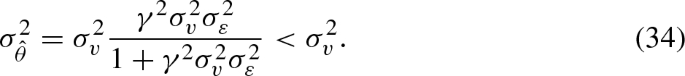
It is also interesting to consider the condition under which agents put more weight on their private information than on prices, i.e., \(\alpha >1-\alpha \) , which requires \(\gamma ^{2}\sigma _{v}^{2}\sigma _{\varepsilon }^{2}>1\). When \(\sigma _{v}^{2}\sigma _{\varepsilon }^{2}\) is small, thus, agents pay little attention to their private signal: this happens when either the variance of the supply is low (and thus aggregate noise is low and prices are more informative), or when private information is very precise (because, as explained above, this enhances the informativeness of prices). An important feature of the Bayesian equilibrium is that \(\alpha \) is not a free parameter but depends instead on the deep structure of the model, as shown by (38).
The limiting results on the optimal use of information just discussed have implications also for traders’ demand. In fact, rewriting (29) as
with \(a=\frac{\alpha }{\gamma \sigma _{{\hat{\theta }}}^{2}}=\left( \gamma \sigma _{v}^{2}\right) ^{-1}\), it can be seen that \(\sigma _{v}^{2}\rightarrow 0\) implies \(s^{i}\rightarrow \infty \): as private information becomes infinitely precise, the demand’s response to deviations of prices from the (increasingly precise) signal grows without bounds. In the limit, the only equilibrium possible is one where prices are equal to the fundamental value.
Note instead that as \(\sigma _{\varepsilon }^{2}\rightarrow 0,\) prices become infinitely precise through the aggregation of private information but individual demands do not depend on the volatility of supply: agents demand the same quantity, irrespective of \(\sigma _{\varepsilon }^{2}\). As the volatility of supply decreases towards zero, in fact, \(\alpha \rightarrow 0\) , which makes agents respond less and less to deviations of their private signal from prices; at the same time, though, the conditional variance of the return on the asset also decreases, which increases the demand of risk averse agents, with the result that the amount demanded is constant with respect to \(\sigma _{\varepsilon }^{2}\).
4 Time-varying fundamental
Results derived in the multi-period setting with \(\sigma _{z}^{2}=0\) follow from the accumulation of information, as conditionally independent signals on a constant fundamental are received sequentially over time. A crucial element for this result is the fact that the fundamental is constant over time. If the fundamental was instead time-varying, agents would need discount past information more heavily, which would affect the precision of their estimates over time and the informational content of prices. To investigate these issues I now consider the general case with \(\sigma _{z}^{2}>0\), so the fundamental changes over time, following a random walk process.
The ensuing system gives rise to a state-space model where (7) represents the state equation and (8) an observation equation. Given such state-space system, the optimal way to track the evolution of \(\theta _{t}\) for agents, if there was no other information available, would be through the use of a Kalman filter on the series \( \{x_{j}^{i}\}_{j=1}^{t}\), which is known to minimize the mean square error of the estimated unknown state when all noise is Gaussian and the model is linear as in this case. In terms of notation, \({\bar{x}}_{t}^{i}\) represents the estimate of the fundamental at time t based on the Kalman filter on exogenous information only; \(\beta _{t}^{-1}\) is the variance of the error of such estimate; and \(k_{t}^{x}\) is the Kalman gain, which governs the way new information is factored into the estimates of the fundamental over time.
The Kalman filter (see, e.g., Elliott et al. (1995)) recursions to compute posterior mean and variance of the fundamental based on exogenous information only are given by
with \({\bar{x}}_{0}^{i}=0\) and \(\beta _{0}=0\) (that is, \({\bar{x}} _{1}^{i}=x_{1}^{i}\), because of a flat prior). It is straightforward to show that (40)–(41) reduce to (11)–(12), with \(k_{t}^{x}=t^{-1}\), if \(\sigma _{z}^{2}=0\).Footnote 8
The Kalman filter estimate can also be rewritten in a non-recursive way, which highlights the relationship between gains and weights, as
with
where \(k_{j}^{x}\) is the Kalman gain given by (42). It can be shown that \(\sum _{j=1}^{t}h_{j}^{t}=1\).Footnote 9
If one assumes that agents use only exogenous private information, then
Substituting into the price equation, with \(\sigma _{{\hat{\theta }} _{t}}^{2}=\beta _{t}^{-1}\), one obtains
with conditional variance
In order to understand the informational content of the Kalman estimate, \( {\hat{\theta }}_{t}^{i}\), and thus of prices, one can solve recursively from (40):
Integrating then over agents and using Eq. (47) for prices
This equation shows how the noise in prices displays both serial correlation and cross correlation with the process noise. Still, this does not preclude to use prices as an additional source of information. Their very use, though, alters the prediction for the fundamental, and thus prices themselves. In particular, current prices would also include past aggregate supply shocks, another source of serial correlation. As before, en equilibrium in the use of information must be found.
To see this point, assume in equilibrium a signal \({\tilde{p}}_{t}\) from prices can be derived, in the form
Writing \(y_{t}^{i}=\left[ x_{t}^{i}\ {\tilde{p}}_{t-1}\right] ^{\prime }\) , with
the Kalman filter estimate for the fundamental could then be represented as
Here \(q_{j}^{t}\) is a \(1\times 2\) vector, to be determined, which gives the relative weight on the two signals, exogenous and endogenous, and depends on current and past Kalman gains. Then prices would be given by
Prices would thus include the whole history of fundamental innovations \(z_{j} \),Footnote 10 and of exogenous supply shocks \(\varepsilon _{j}\) (through \({\tilde{p}}_{j}\)). One, though, can remove the serial correlations due to past price signals by defining \({\tilde{p}}_{t}\) as follows
with
The signal \({\tilde{p}}_{t}\) has thus the form (53), but with all the \(\tau _{j}^{t}=0\) except for \(\tau _{t}^{t}\). In order to find the explicit representation of all coefficients in \({\tilde{p}}_{t}\), one needs to write the Kalman filter parameters \(q_{j}^{t}\) in terms of variances and covariances of state and signals.
As agents cannot observe contemporaneous prices when forming beliefs about the fundamental, their endogenous time\(-t\) signal for \(\theta _{t}\) is represented by \({\tilde{p}}_{t-1}\), which can be rewritten as
with \(\psi _{t-1}^{t-1}=\sum _{j=1}^{t-1}q_{j,1}^{t-1}\), which implies that the coefficient in \({\tilde{p}}_{t-1}\) on \(z_{t-1}\) is \(-1\).
What (56) shows is that it is possible for agents, using only known quantities (past price signals and Kalman gains), to remove the serial correlation in prices that comes from using endogenous signals in the Kalman filter recursion. It is not possible instead to remove the serial correlation and the cross correlation with the state noise that comes from innovations in the fundamental, as these are unobservable to agents.
The remaining noise in the price signal \({\tilde{p}}_{t}\) displays both t-step serial correlation and t-step cross correlation with the process noise, with correlation structures changing over time and increasing in length. Li et al. (2000) shows how to deal with arbitrary correlation structures inside a Kalman filter setting, and I follow their approach in my analysis, adapting it to the present setting. The appropriate Kalman filter recursions are shown in Appendix 6.5. In Appendix 6.6 I then show that this procedure reduces to the one presented in Sect. 3 for \(\sigma _{z}^{2}=0\).
Because of the endogenous correlation structures, the long-run behavior of this modified Kalman filter cannot be analysed analytically. I therefore use numerical simulations to investigate it, and in particular to understand long run weights on public versus private information.
First, note that, from (60), the conditional variance of \( {\tilde{p}}_{t-1}\) can be written as
The question then is whether this conditional variance: i) converges to a positive constant, so that agents keep using both endogenous and exogenous information; ii) converges to zero, so that agents asymptotically use only information from prices; or iii) diverges, so that agents asymptotically use only private signals. This depends on the sum of the squares coefficients on the fundamental innovations \(z_{i}\) in \({\tilde{p}}_{t}\).
I thus implement numerically the algorithm presented in Appendix 6.5, for a wide range of parameterizations for the deep parameters \(\gamma \), \(\sigma _{z}^{2}\), \(\sigma _{\varepsilon }^{2}\), \( \sigma _{v}^{2}\). Numerical simulations show that in all cases:
-
1.
The sum of coefficients on the fundamental innovations in the price signal, \(\frac{\sum _{j=1}^{t-1}\psi _{j}^{t}}{\sum _{j=1}^{t}q_{j,1}^{t}}\), converges over time to a constant. The number of terms increases with t, but their sum remains always finite and converges to a constant.
-
2.
The Kalman gain \(K_{t}\) converges over time to a constant vector: this means that weights on public and private signals converge to positive constants.
-
3.
The posterior variance of the Kalman filter estimate, \(\sigma _{{\hat{\theta }}_{t}}^{2}\), converges also to a constant.
-
3.
Whether the equilibrium weight on the endogenous signal is larger or smaller than that on the exogenous one depends on the relative values of the structural parameters \(\gamma ,\sigma _{z}^{2},\sigma _{\varepsilon }^{2},\sigma _{v}^{2}\). In particular, larger \(\gamma \), \(\sigma _{\varepsilon }^{2}\) and \(\sigma _{z}^{2}\) increase the conditional variance of the price signal, as it can be seen by (61), and thus reduce the Kalman gain on \({\tilde{p}}_{t-1}\) relative to the one on \( x_{t}^{i} \); \(\sigma _{v}^{2}\) has instead the opposite effect, as it affects negatively the precision of the exogenous signal.
In equilibrium agents thus use both private exogenous and public endogenous information with fixed weights, as the precision of both signals converges over time to a constant.
Proposition 2
In the setting presented in Sect. 4, if the information set used by agents is given by \({\mathcal {I}}_{t}^{i}=\left\{ p^{t-1},x^{i,t}\right\} \) and agents use their information efficiently through a Kalman filter, the precision of agents’ beliefs about the fundamental converges over time to a positive constant.
These results show how it is possible for agents to use prices as endogenous signals in case of a time-varying fundamental, and demonstrate that both endogenous and exogenous information are used in equilibrium by agents. The Grossman–Stiglitz paradox thus does not emerge, even asymptotically, when the fundamental changes over time.
4.1 Alternative information sets
It is instructive to compare the above results with the outcome under alternative information sets available to agents. In particular, two information sets seem particularly relevant: the first is when agents can only observe exogenous signals (because, for example, equilibrium prices for past periods when trade did not take place were not announced), that is
and the second is when agents can observe the whole history of prices but only the current exogenous signal (because, for example, individual agents can take part in only one round, but past equilibrium prices are announced), that is
In both cases, the asymptotic behavior of the system can be analysed analytically, as there are no endogenous correlation structures to be accounted for in the signal extraction problem, and so it is possible to gain further insights into results from the previous Section.
In the first case, with \({\mathcal {I}}_{t}^{i}=\left\{ x^{i,t}\right\} \), posterior mean and variances are given by (40)–(42), with \({\hat{\theta }}_{t}^{i}={\bar{x}}_{t}^{i}\) and \(\sigma _{{\hat{\theta }} _{t}}^{2}=\beta _{t}^{-1}\). Prices would then be given by (51):
In terms of the asymptotic variance of the estimation error, this can be found by the limit behavior of the non-linear difference Eq. (41), given by its fixed point, that isFootnote 11
The gain coefficient in the Kalman filter, determining the weighting structure on past signals, would also converge to a constant, with
It can thus be seen that the precision of agents’ estimates about the fundamental would converge to a constant, as the precision of their cumulative signal remains finite over time. This is a well known property of the Kalman filter with a time-invariant state-space and exogenous information.
Remark 1
In the setting presented in Sect. 4, if the information set used by agents is given by \({\mathcal {I}}_{t}^{i}=\left\{ x^{t,i}\right\} \) and agents use their information efficiently through a Kalman filter, the precision of agents’ beliefs about the fundamental converges over time to a positive constant.
In the second case, with \({\mathcal {I}}_{t}^{i}=\left\{ p^{t-1},x_{t}^{i}\right\} \), agents would use past prices and current exogenous information. Assuming that \({\tilde{p}}_{j}\), \(j=1,...,t-1\) is an unbiased signal for \(\theta _{j}\) (to be verified), agents at any time \(t>1\) could use past price signals to construct an estimate for \(\theta _{t-1}\), denoted \({\hat{\theta }}_{t-1}^{p}\) (common for all agents because based only on public information), which in non-recursive form is given by
with weights \(l_{j}^{t}\) depending on the Kalman gains.
Agents can then take \({\hat{\theta }}_{t-1}^{p}\) as their prior and use the current observation \(x_{t}^{i}\) to update their beliefs for \(\theta _{t}\). The ensuing new posterior mean for each agent i, \({\hat{\theta }}_{t}^{i}\), would be
with \({\tilde{k}}_{t}\), the Kalman gain at time t, given by
and posterior variance
with \(\sigma _{{\hat{\theta }}_{t-1}^{p}}^{2}\) given recursively by
and representing the variance of the estimate error from \({\hat{\theta }} _{t-1}^{p}\).
Prices would then be equal to
As the estimate \({\hat{\theta }}_{t-1}^{p}\), given by (67), is common across agents, each agent can construct the endogenous signal
with conditional variance
The price signal \({\tilde{p}}_{t}\) is thus conditionally independent, which confirms the assumption made before and validates the filtering procedure.Footnote 12 Note that here, contrary to the case where past exogenous information is available, the price signal does not include any serial or cross correlation with the process noise, as all correlations induced by the filtering procedure can be removed, since they derive from public and common information. It is the use of past private information that creates additional correlation structures in the public signal, which cannot be removed by agents and need to be accounted for through a modified Kalman filter.
To understand the asymptotic weights on public and private signals, the conditional variance of \({\tilde{p}}_{t}\) must be computed. Using (69) and (70) to compute \( {\tilde{k}}_{t}^{-1}\sigma _{{\hat{\theta }}_{t}}^{2}\) in (74) gives
which leads to \(\sigma _{{\tilde{p}}_{t}}^{2}=\gamma ^{2}\left( \sigma _{v}^{2}\right) ^{2}\sigma _{\varepsilon }^{2}\equiv \sigma _{{\tilde{p}}}^{2}\) , constant.
The variance of the Kalman filter estimate from prices only, \(\sigma _{{\hat{\theta }}_{t-1}^{p}}^{2}\) depends only on its past value, on \(\sigma _{z}^{2}\) and on \(\sigma _{{\tilde{p}}}^{2}\), as shown in (71), and converges over time to a constant.
In terms of the variance of the posterior estimate \({\hat{\theta }}_{t}^{i}\) after the exogenous signal is observed, its limit behavior is given, using (76), by
where, by (69),
To compute \(\lim _{t\rightarrow \infty }\sigma _{{\hat{\theta }}_{t-1}^{p}}^{2}\) one needs to find the limit behavior of the non-linear difference Eq. (71), with \(\sigma _{{\tilde{p}}}^{2}=\gamma ^{2}\left( \sigma _{v}^{2}\right) ^{2}\sigma _{\varepsilon }^{2}\) constant as shown in (75), given by
Putting together (77), (78) and (79) leads to a constant asymptotic variance of the Kalman estimation error
The asymptotic variance of the estimation error, \(\sigma _{{\hat{\theta }} _{t}}^{2}\), thus converges also in this case to a constant, and so does the Kalman gain \({\tilde{k}}_{t}\). As the precision of the posterior remains finite, the conditional variance of prices remains strictly positive and the price signal \({\tilde{p}}_{t}\) from (74) never becomes fully revealing. Agents continue to use both public endogenous and private exogenous information to infer the fundamental value over time, with weights converging to a constant. Again, the precision of their information remains finite over time.
Proposition 3
In the setting presented in Sect. 4, if the information set used by agents is given by \({\mathcal {I}}_{t}^{i}=\left\{ p^{t-1},x_{t}^{i}\right\} \) and agents use their information efficiently through a Kalman filter, the precision of agents’ beliefs about the fundamental converges over time to a positive constant.
Note finally that in the case of a constant fundamental (i.e., \(\sigma _{z}^{2}=0\)), with any of the three information sets considered prices would become asymptotically fully revealing (though at different rates). It was shown in Sect. 3 for \({\mathcal {I}}_{t}^{i}=\left\{ p^{t-1},x^{i,t}\right\} \) and it is trivial to prove the result if \({\mathcal {I}}_{t}^{i}=\left\{ x^{i,t}\right\} \), using (14). If instead \( {\mathcal {I}}_{t}^{i}=\left\{ p^{t-1},x_{t}^{i}\right\} \), this result can be proved using (86), with \(\beta _{t}=\sigma _{v}^{-2}\) (since only the current exogenous signal is now available): \(\lim _{t\rightarrow \infty }\omega _{t}=\infty \), which also implies that \(\lim _{t\rightarrow \infty }\alpha _{t}=0\).
5 Conclusions
This paper has investigated the ability of prices to convey information about the fundamental value of an asset in a setting with sequential signals and Bayesian learners.
It has been noted before (see Vives 1995b) that information accumulation can lead to a dynamic version of the Grossman–Stiglitz paradox, as asymptotically price signals become fully revealing and traders stop using private signals. We have seen here that such result extends to a setting where information accumulates also through private signals, as long as the fundamental value is constant over time. With a constant fundamental, in fact, as time goes on and more signals are received, the precision of both private and public cumulative signals increases without bounds, though at different rates: the precision of public signals grows at a faster rate, so agents over time rely more and more on the endogenous rather than the exogenous information and asymptotically disregard private information altogether.
The fact that asymptotically price signals become fully revealing and traders stop using private ones does not repropose the problem exposed in the famous Grossman–Stiglitz paradox because it is an asymptotic outcome with information accumulation: as agents progressively switch from private to public information, the precision of price signals increases and they reveal more of the fundamental. In the limit, there is no longer any need to acquire further information on the constant fundamental through exogenous signals.
With a time-varying fundamental, instead, the role of prices as a source of information is complicated by the endogenous and time-varying serial and cross correlation structures that emerge. Nevertheless, I have shown how agents can still use prices as a source of information, through a modified Kalman filter with arbitrary correlations. As the precision of the endogenous signal in this case remains finite and converges to a constant, agents keep using both exogenous and endogenous information over time, with relative weights converging to a constant.
The central theme of this paper is the relationship between the informational content of prices and the nature of the underlying fundamental. Only if the fundamental is constant, Bayesian learning implies an increasing precision of agents’ beliefs and asymptotically fully revealing prices. With a changing fundamental, instead, the use of prices as endogenous signals is complicated by the use of past exogenous information. Correlation structures induced by the innovations in the fundamental need to be taken into account in order to extract information from prices: we have seen how this can be done and shown that prices, while still being informative, never become fully revealing.
Notes
Basak and Chabakauri (2010) show that dynamic mean-variance portfolio choices are not dynamically consistent. While this is an important issue, mean-variance behavior is still commonly assumed as it leads to analytically tractable demand functions. In the present setting, as agents effectively solve a series of one-period problems, this issue does not arise.
One could equivalently assume risk averse agents with CARA utility

Maximizing the expected value of \(U(R_{t}^{i})\) is equivalent to maximizing (1), the certainty equivalent, assuming a CARA utility function and normal random returns.
Such conditional variance is common across agents, given the informational assumptions made. In particular, while agents receive heterogeneous private information, the precision of such information is common across agents.
Note that the fundamental can be negative, and so do prices. Such feature can be justified by assuming that there is no free disposal of the risky asset. This simplifies the set up, as it avoids having a truncation in the support of agents’ beliefs.
This will not be true for the case with a time-varying fundamental, where individual signals need to be merged together through a Kalman filter procedure.
The formulation used here, with separate cumulative signals, has the advantage of allowing one to see the evolution of the precision of public and private information separately, and how this affects relative weights.
Note that using (22), with \(\omega _{0}=0\) and \({\bar{p}}_{0}=0\), at time \(t=1\), \(p_{1}\) reduces to (35). While the price is the same, here the precision of agents’ beliefs is higher than in that case at \(t=1\), when it was \(\beta _{1}^{2}=\sigma _{v}^{-2}\), since they can here use current equilibrium prices in their inference. It is in fact straightforward to show that now
The variance of prices is in fact quadratic in \(\sigma _{v}^{2}\): see (36).
With \(\sigma _{z}^{2}=0\), the fundamental is constant, so there is no need to track changes and thus \(k_{t}=t^{-1}\); with \(\sigma _{v}^{2}=0\), instead, the fundamental is perfectly observable and there is no need to filter out the noise, so \(k_{t}=1\).
The estimate \({\bar{x}}_{t}^{i}\) can equivalently be obtained by using generalized least squares on the data \(\left\{ x_{j}^{i}\right\} _{j=1}^{t}\) , with each \(x_{j}^{i}\) representing a signal for \(\theta _{t}\).
These would enter both through the exogenous signals \(x_{j}^{i}\) and the endogenous ones \(p_{j}^{i}\).
Only the positive root is meaningful for a variance.
If one assumes that agents take part in only one round, at each time t agents would need to reconstruct the whole history of \(\left\{ {\tilde{p}} _{j}\right\} _{j=1}^{t-1}\). This can easily be done by computing recursively all past \({\tilde{k}}_{j}\) and \({\hat{\theta }}_{j-1}^{p}\), \(j>1\), using (67) and (69).
Following usual conventions in the Kalman filter literature, \({\hat{\theta }}_{t\shortmid t-1}^{i}\) represents the prediction based on information up to time \(t-1\), and \({\hat{\theta }}_{t\shortmid t}^{i}\) is the posterior mean after time t information has been included. Similarly, \(\sigma _{{\hat{\theta }}_{t|t-1}}^{2}\) is the error variance associated to \({\hat{\theta }}_{t\shortmid t-1}^{i}\) and \(\sigma _{{\hat{\theta }}_{t|t}}^{2}\) the error variance associated with \({\hat{\theta }}_{t\shortmid t}^{i}\). In terms of the notation in the main text, \({\hat{\theta }}_{t}^{i}={\hat{\theta }}_{t\shortmid t}^{i}\) and \(\sigma _{{\hat{\theta }}_{t}}^{2}=\sigma _{{\hat{\theta }}_{t\shortmid t}}^{2}.\)
With \(\Psi _{t-1}=0\) and \(\Omega _{t}=0,\forall t\), this recursion reduces to the standard Kalman filter.
At time \(t=1\),

so \(\phi _{1}^{1}=-1\) and \(\eta _{1}=-\gamma \sigma _{v}^{2}.\)


References
Allen, F., Morris, S., Shin, H.S.: Beauty contests and iterated expectations in asset markets. Rev Financ Stud 19(3), 719–752 (2006)
Amador, M., Weill, P.-O.: Learning from private and public observations of others’ actions. J Econ Theory 147, 910–940 (2012)
Basak, S., Chabakauri, G.: Dynamic mean-variance asset allocation. Rev Financ Stud 23, 2970–3016 (2010)
Branch, W.A., Evans, G.W.: Learning about risk and return: a simple model of bubbles and crashes. Am Econ J: Macroecon 3, 159–191 (2011)
Diamond, D.W., Verrecchia, R.E.: Information aggregation in a noisy rational expectations economy. J Financ Econ 9, 221–235 (1981)
Elliott, R.J., Aggoun, L., Moore, J.B.: Hidden Markov Models: Estimation and Control. Springer-Verlag, New York (1995)
Grossman, S.: On the efficiency of competitive stock markets where traders have diverse information. J Financ 31, 573–585 (1976)
Grossman, S.: Further results on the informational efficiency of competitive stock markets. J Econ Theory 18, 81–101 (1978)
Grossman, S., Stiglitz, J.: On the impossibility of informationally efficient markets. Am Econ Rev 70, 393–408 (1980)
Hellwig, M.F.: On the aggregation of information in competitive markets. J Econ Theory 22, 477–498 (1980)
Jackson, M.: Equilibrium, price formation, and the value of private information. Rev Financ Stud 4, 1–16 (1991)
Kasa, K., Walker, T.B., Whiteman, C.H.: Heterogeneous beliefs and tests of present value models. Rev Econ Stud 81, 1137–1163 (2014)
Kyle, A.S.: Continuous auctions and insider trading. Econometrica 53, 1315–1335 (1985)
Kyle, A.S.: Informed speculation with imperfect competition. Rev Econ Stud 56, 317–356 (1989)
Li, X.R., Han, C., Wang, J.: Discrete-time linear filtering in arbitrary noise. In: Proceedings of the 39th IEEE Conference on Decision and Control 2, pp. 1212–1217 (2000)
Mele, A., Sangiorgi, F.: Uncertainty, information acquisition, and price swings in asset markets. Rev Econ Stud 82, 1533–1567 (2015)
Nimark, K.P.: Dynamic Higher Order Expectations. Working paper, mimeo (2017)
Sargent, T.J.: Equilibrium with signal extraction from endogenous variables. J Econ Dynam Control 15, 245–273 (1991)
Townsend, R.M.: Forecasting the forecasts of others. J Polit Econ 91, 546–588 (1983)
Vives, X.: How fast do rational agents learn? Rev Econ Stud 60, 329–347 (1993)
Vives, X.: Short-term investment and the information efficiency of the market. Rev Financ Stud 8, 125–160 (1995a)
Vives, X.: The speed of information revelation in a financial market mechanism. J Econ Theory 67, 178–204 (1995b)
Vives, X.: On the possibility of informationally efficient markets. J Eur Econ Assoc 12, 1200–1239 (2014)
Author information
Authors and Affiliations
Corresponding author
Ethics declarations
Conflict of interest
The authors declare that they have no conflict of interest.
Additional information
Publisher's Note
Springer Nature remains neutral with regard to jurisdictional claims in published maps and institutional affiliations.
Appendix
Appendix
1.1 Proof of Proposition 1
Proof
The proof consists in deriving the limiting outcomes of the system as \( t\rightarrow \infty \). Using (11), by the law of large numbers
and from (12)
That is, by the law of large numbers, the sample mean converges in probability to the mean of the distribution and its variance goes to zero.
Consider then \(\sigma _{{\hat{\theta }}_{t}}^{2}=\frac{1}{\beta _{t}+\omega _{t-1}}\). Since \(\lim _{t\rightarrow \infty }\beta _{t}=\infty \), and by definition \(\omega _{t}\ge 0\), \(\forall t\), it follows from (20 ) that
and from (25)
This last result also implies, from (16), that
Finally, since
it follows that
Then clearly,
Looking then at prices, starting from (21) and noting results (83) and (88)
In order to compute \({{\,\mathrm{plim}\,}}_{t\rightarrow \infty }{\bar{p}}_{t}\), one can make use of a version of the weak law of large numbers for independent but not identically distributed random variables, which states that given \( \{X_{j}\}\) a sequence of independent but not identically distributed random variables, if \(lim_{t\rightarrow \infty }\frac{1}{t^{2}}Var[ \sum _{j=1}^{t}X_{j}]=0\), then, for any \(\varepsilon >0,\)
First, I define \(X_{j}^{t}=t\frac{\sigma _{{\tilde{p}}_{j}}^{-2}{\tilde{p}}_{j}}{ \sum _{n=1}^{t}\sigma _{{\tilde{p}}_{n}}^{-2}}.\) Then \({\bar{p}}_{t}=\frac{1}{t} \sum _{j=1}^{t}X_{j}^{t}.\) Note that \(E{\bar{p}}_{t}=t^{-1} \sum _{j=1}^{t}EX_{j}^{t}=\frac{t}{t}\sum _{j=1}^{t}\frac{E\sigma _{{\tilde{p}} _{j}}^{-2}{\tilde{p}}_{j}}{\sum _{n=1}^{t}\sigma _{{\tilde{p}}_{n}}^{-2}} =\sum _{j=1}^{t}\frac{\sigma _{{\tilde{p}}_{j}}^{-2}}{\sum _{n=1}^{t}\sigma _{ {\tilde{p}}_{n}}^{-2}}\theta =\theta .\) Thus, in order to prove that \({\bar{p}} _{t}\) converges in probability to \(\theta \), it needs to be shown that \( t^{-2}Var[\sum _{j=1}^{t}X_{j}^{t}]\rightarrow 0.\) Note that, since \( X_{j}^{t} \) are independent over j,
and thus
Note finally that the denominator in the last expression, \( \sum _{n=1}^{t}\sigma _{{\tilde{p}}_{n}}^{-2}\), is equal to \(\omega _{t}\), which, as already established, converges to \(\infty \) as \(t\rightarrow \infty \). This concludes the proof that
\(\square \)
1.2 Normal priors
An assumption used throughout this paper is that of an uninformative prior for agents at time 1, before observing any inforation, which simplifies some of the analysis and derivation of key equations. I show here that this assumption is in fact innocuous for results in this paper.
Using the static setting of Sect. 3.1, if one assumes that Nature draws from a Normal distribution with some constant mean \({\bar{\theta }}\) and standard deviation \(\sigma _{\theta }\), then agents have an informative prior to use in their inference. In this case, then
with
The new price equation would be
with
The conditional variance of prices would thus be given by
Substituting into the previous equation for \(\mu \),
and for \(\alpha \),
One can see that as \(\sigma _{\theta }^{2}\rightarrow \infty \), \(\mu \rightarrow 0\) and \(\alpha \rightarrow \frac{\gamma ^{2}\sigma _{v}^{2}\sigma _{\varepsilon }^{2}}{1+\gamma ^{2}\sigma _{v}^{2}\sigma _{\varepsilon }^{2}}\), thus giving back the framework with uninformative prior.
The important result here is that, as it was the case with an uninformative prior, as \(\sigma _{v}^{2}\rightarrow 0\), \(\alpha \) (and now also \(\mu \)) \( \rightarrow 0\), so agents rely only on prices in forming beliefs about the fundamental. As results with sequential signals and information accumulation build on this feature of the model, by which the precision of public information improves more than proportionally with the precision of the exogenous one, this shows that such results would carry out also in the case of an informative prior. The assumption of an uninformative prior is thus inconsequential for the analysis in this paper.
1.3 Derivation of optimal \(\alpha \) with private and public signals
The optimal linear weight on the two signals, \(\alpha \), can be obtained by solving the problem
with
Minimizing (97) subject to (98) leads to the first order condition
whose solution implies
Given that prices and exogenous signals do not covariate (since the noise in the exogenous signal is averaged out by aggregation), this reduces to
1.4 Derivation of the equilibrium price
Substituting (103) into (32) leads to
and therefore
1.5 Recursive filtering with arbitrary noise
This exposition is taken and adapted from Li et al. (2000). Consider the general system analysed in Sect. 4, represented by
with \(H=[1\) \(1]^{\prime }\), \(y_{t}^{i}=[x_{t}^{i}\) \({\tilde{p}}_{t-1}]^{\prime }\) and \(w_{t}^{i}=[v_{t}^{i}\) \({\tilde{w}}_{t}]\), where \({\tilde{w}}_{t}\) \( \equiv {\tilde{p}}_{t-1}-\theta _{t}\). Process and measurement noise are zero mean but colored, with arbitrary covariance matrices
Moreover, \(\{z\}\) and \(\{w\}\) are arbitrarily correlated with each other, with cross-covariances
The initial state is here uncorrelated with state and measurement noise at any time. Following Theorem 3 in Li et al. (2000), it is possible to write the recursive filter for this system as follows:Footnote 13
-
1.
Initialization: \({\hat{\theta }}_{1\shortmid 1}^{i}=x_{1}^{i};\sigma _{ {\hat{\theta }}_{1\mid 1}}^{2}=\sigma _{v}^{2}.\)
For \(t>1\):
-
2.
Prediction:
$$\begin{aligned} {\hat{\theta }}_{t\shortmid t-1}^{i}= & {} {\hat{\theta }}_{t-1\shortmid t-1}^{i} \end{aligned}$$(107)$$\begin{aligned} \sigma _{{\hat{\theta }}_{t\mid t-1}}^{2}= & {} \sigma _{{\hat{\theta }}_{t-1\mid t-1}}^{2}+Q_{t-1}+2\Psi _{t-1} \end{aligned}$$(108)with
$$\begin{aligned} \Psi _{t-1}=\Psi _{t-1|t-1}^{t-1} \end{aligned}$$(109)and \(\psi _{n|j}^{t-1}\) given by the Kalman filter, for \(n=2,...,t-1\)
$$\begin{aligned} \Psi _{n|n-1}^{t-1}= & {} \Psi _{n-1|n-1}^{t-1}+Q_{n-1,t-1} \end{aligned}$$(110)$$\begin{aligned} \Psi _{n|n}^{t-1}= & {} \Psi _{n|n-1}^{t-1}+K_{n}\left( -C_{t-1,n}^{\prime }-H\Psi _{n|n-1}^{t-1}\right) \end{aligned}$$(111)with initial value \(\psi _{1|1}^{t-1}=0\).
-
3.
Update:
$$\begin{aligned} {\hat{\theta }}_{t\shortmid t}^{i}= & {} {\hat{\theta }}_{t\shortmid t-1}^{i}+K_{t} \left[ y_{t}^{i}-H{\hat{\theta }}_{t\shortmid t-1}^{i}\right] \end{aligned}$$(112)$$\begin{aligned} \sigma _{{\hat{\theta }}_{t\mid t}}^{2}= & {} \sigma _{{\hat{\theta }}_{t\mid t-1}}^{2}-K_{t}S_{t}K_{t}^{\prime } \end{aligned}$$(113)with \(K_{t}\) and \(S_{t}\) given respectively by
$$\begin{aligned} K_{t}= & {} \left( \sigma _{{\hat{\theta }}_{t\mid t-1}}^{2}H_{t}^{\prime }+\Omega _{t}\right) S_{t}^{-1} \end{aligned}$$(114)$$\begin{aligned} S_{t}= & {} H\sigma _{{\hat{\theta }}_{t\mid t-1}}^{2}H^{\prime }+H_{t}\Omega _{t}+\left( H\Omega _{t}\right) ^{\prime }+R_{t} \end{aligned}$$(115)with
$$\begin{aligned} \Omega _{t}=\Omega _{t|t-1}^{t} \end{aligned}$$(116)and \(\Omega _{n|j}^{t}\) given recursively by the Kalman filter, for \( n=2,...,t\) (but the update for \(\Omega _{n|n}^{t}\) is needed and carried out only up to \(n=t-1\))
$$\begin{aligned} \Omega _{n|n-1}^{t}= & {} \Omega _{n-1|n-1}^{t}+C_{n-1,t} \end{aligned}$$(117)$$\begin{aligned} \Omega _{n|n}^{t}= & {} \Omega _{n|n-1}^{t}+K_{n}\left( -R_{nt}-H\Omega _{n|n-1}^{t}\right) \end{aligned}$$(118)with initial value \(\Omega _{1|1}^{t}=0\).
The differences with the standard Kalman filter are given by the terms \(\Psi _{t-1}\) and \(\Omega _{t}\), due to time and cross correlation of state and measurement noises.Footnote 14 The computation of these terms requires two nested filters within the main recursion. First, note that \(Q_{nj}=\sigma _{z}^{2}\) for \(n=j\) and 0 otherwise.
In the context of the present model, the variance covariance matrices required to compute \(\Psi _{t-1}\) and \(\Omega _{t}\) can be derived as follows. Rewriting (60) as
with
one can define all the endogenous serial and cross correlations needed for the recursion. In particular
with
and \(\delta _{jt}\) denoting the Kronecker delta.
Given that \(Q_{n<j,j}=0\) and \(C_{t-1,j}=[0\)\(0]^{\prime },\forall j\), the first nested Kalman filter recursion (110)–(111) reduces to
and given that \(\psi _{1|1}^{t-1}=0\), this implies that \(\Psi _{t-1|t-1}^{t-1}=0,\forall t>1\). This simplification is due to the fact that in this system there is no serial correlation in the state noise, and no cross correlation between the current innovation in the state (\(z_{t-1}\)) and past measurements up to \(y_{t-1}^{i}\). The key term introduced by the endogeneity of prices and due to the serial correlation in the noise in \( {\tilde{p}}_{t}\) and the cross correlation of such noise with the noise in the state, is thus \(\Omega _{t}\), the computation of which requires the computation of the \(\phi _{j}^{t-1}\) and \(\eta _{t-1}\) coefficients in (119), for \(t>1\).Footnote 15 Deriving the equivalence between weights and gains in the Kalman filter gives
Using then (120) and (121), one can derive the required covariance matrices \(R_{j,t}\) and \(C_{j,t}\).
1.6 Kalman filter updating equivalence
I show here that, for \(\sigma _{z}^{2}=0\), the weight put on new information under the Kalman filter recursion is the same as the one in the learning algorithm proposed in Sect. 3.
With \(\sigma _{z}^{2}=0\), the modified Kalman filter algorithm presented in Appendix 6.5 reduces to a standard Kalman filter algorithm, as there is no longer any serial correlation in \({\tilde{p}}_{t}\), nor any cross correlation between \({\tilde{p}}_{t}\) and the (constant) fundamental. The relevant equations are thus simplified to
with
Using the fact that
it is straightforward to compute the weight put at time t on the new signals \(x_{t}^{i}\) and \({\tilde{p}}_{t-1}\), given by the Kalman gain
These are the same weights put on new information under the algorithm proposed in Sect. 3. In fact, using (18), (20) and (11)
so the weight on new private information \(x_{t}^{i}\) is given by \(\sigma _{ {\hat{\theta }}_{t}}^{2}\sigma _{v}^{-2}\). Using the fact that
this implies
which is the same weight on private information implied by the Kalman filter. Using the same steps, it is straightforward to prove the equivalence for the weight put on the price signal.
Rights and permissions
Open Access This article is licensed under a Creative Commons Attribution 4.0 International License, which permits use, sharing, adaptation, distribution and reproduction in any medium or format, as long as you give appropriate credit to the original author(s) and the source, provide a link to the Creative Commons licence, and indicate if changes were made. The images or other third party material in this article are included in the article’s Creative Commons licence, unless indicated otherwise in a credit line to the material. If material is not included in the article’s Creative Commons licence and your intended use is not permitted by statutory regulation or exceeds the permitted use, you will need to obtain permission directly from the copyright holder. To view a copy of this licence, visit http://creativecommons.org/licenses/by/4.0/.
About this article

Cite this article
Berardi, M. Learning from prices: information aggregation and accumulation in an asset market. Ann Finance 17, 45–77 (2021). https://doi.org/10.1007/s10436-020-00378-w
Received:
Accepted:
Published:
Issue Date:
DOI: https://doi.org/10.1007/s10436-020-00378-w