
Abstract
This paper employs mechanism design to examine how imperfect legal enforcement impacts simultaneously the availability of credit for investment and interest rates. The analysis combines limited commitment, which encapsulates the idea that courts are imperfect, and asymmetric information about cash flows, which makes debt contracts optimal. Costly use of courts may be optimal, which differs from most limited commitment models, where punishments are merely threats, never actually applied in optimal arrangements. Paradoxically, liquidation by courts only happens in optimal arrangements when courts are imperfect. Credit constraints emerge, but even credit-constrained individuals do not borrow as much as they can. Consistent with stylized facts, wealthier individuals borrow at lower interest rates and run larger-scale enterprises. The reliability of courts has a positive effect on the scale of projects. However, its effect on interest rates is more subtle and depends on the degree of curvature of the production function.


Notes
The term “ bank spread” is used here to define the difference between lending interest rates and deposit interest rates, as reported by the IMF. See Laeven and Majnoni (2005).
Gennaioli (2013) focuses on the decision process within courts, and frictions that potentially generate enforcement risk. The model in the current paper simply takes some exogenous probability of enforcement failure as a reduced form strategy to consider such frictions.
This feature is typical of costly state verification models (e.g. Townsend 1979), but when randomization is allowed debt contracts are no longer optimal. Krasa and Villamil (2000) show that a combination of costly state verification and renegotiation generate debt contracts even when renegotiation is allowed. Here, debt contracts follow from the fact that cash flows are never observed, and incentive for repayment comes from a discrete threat, liquidation.
Putting it differently, the model economy is a small open economy, so the supply of credit is infinitely elastic.
As reported by Araújo and Rodrigues (2004), microdata from credit markets in Brazil (which is the country with a higher bank spread in the data set used by Laeven and Majnoni 2005) reveal that interest rates are very much dependent on the characteristics of borrowers. In their dataset, bank spreads are considerably higher for small firms and small loans.
Alternative equivalent formulation could characterize as decision variables to be defined in the contracts the discrete choice between default, voluntary liquidation and repayment, \(d\), and the amount of second period transfers \(p,\) and impose an alternative limited commitment constraint that any choice for this decision variable must produce at least the utility of default with zero transfers.
The derivation of these indirect value funcitons is trivial:
$$\begin{aligned} V_{2}^{r}(\theta f(k),p_{r})&= \max \limits _{s_{r}}U(\theta f(k)-p_{r} -s_{r})+\beta U(\theta f(k)+(1+r)s_{r}); \\ V_{2}^{v}(\theta f(k),p_{v})&= \max \limits _{s_{v}}U(\theta f(k)-p_{v} -s_{v})+\beta U((1+r)s_{v});\\ V_{2}^{d1}(\theta f(k),p_{d1})&= \max \limits _{s_{d1}}U(\theta f(k)-p_{d1} -s_{d1})+\beta U((1+r)s_{d1}) \hbox { and}\\ V_{2}^{d2}(\theta f(k),p_{d2})&= \max \limits _{s_{d2}}U(\theta f(k)-p_{d2} -s_{d2})+\beta U(\max \{\theta f(k),ik\}+(1+r)s_{d2}) \end{aligned}$$Setting a value of \(p_{r}\) that is so high that the choice of liquidation or default is always optimal is equivalent to assigning individuals to liquidation or default (that implies liquidation with a positive probability).
This distribution was generated from a histogram of a lognormal distribution with mean 1.1, variance 0.3 and median 1.
Although I found some examples where default did not occur.
To put it differently, the problem is solved with the additional constraint that randomization is not allowed. However, based on numerical exercises, this analysis seems to be at least a good approximation to the solution with randomization allowed. In general as I increase the number of points in the \(\theta \) grid, with its distribution as an approximation of a lognormal, there is randomization for a maximum of 3 values of \(\theta \), between the area in which there is repayment with probability 1 and the area where voluntary liquidation or default are chosen with probability 1. The probability of these few points decreases as the grid becomes finer.
This graph was generated with \(k=1,\, b=0.8,i=0.5,c=0.2,\lambda =0.7,\theta \) has lognormal distribution with \(\mu =1\) and \(\sigma =1\) and \(f(k)=k^{0.5}\).
The interest rates results presented in this section are borrowing interest rates, as defined in (6).
Fig. 8 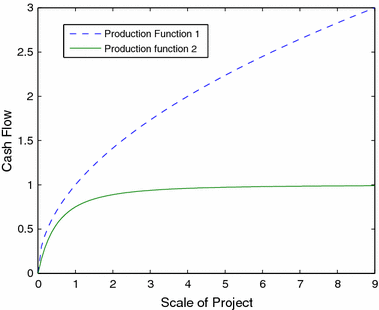
Production functions
Results for different especifications of \(h\) and different values of \(c\) and \(i\) have also been generated and are available from the author upon request. The probability of default and the interest rates increase with the variance of \(\theta \), and decrease with the cost of courts \(c\). Also, the scale of projects tend to be higher as the liquidation value of projects increase. In all specifications, borrowing interest rates are decreasing with wealth and scale is increasing with \(\lambda \).
In the case of different specifications of \(h(\theta )\), the parameters \(\mu \) and \(\sigma \) of the lognormal distribution are chosen so that the expected value of \(\theta \) remains constant.
This prediction is consistent with results presented by Antunes et al. (2014). They construct and calibrate a general equilibrium model with financial and enforcement frictions. When comparing differences in U.S. output per capita to counterfactually high frictions consistent with Brazil, they find that intermediation and enforcement frictions can explain about 20–25 % of the output gap between the two countries.
Note that, from the structure presented in Fig. 1, \(V_{2}^{d1}(y,p)=V_{2}^{v}(y,p+ik)\), and when \(l=1,\, V_{2}^{d2}(y,p)=V_{2}^{v}(y,p)\).

References
Acemoglu, D., Johnson, S., Robinson, J.A.: Institutions as a fundamental cause of long-run growth. Handb. Econ. Growth 1, 385–472 (2005)
Antunes, A., Cavalcanti, T., Villamil, A.: The effects of credit subsidies on development. Forthcoming, Econ. Theory (2014) doi:10.1007/s00199-014-0808-0
Araújo, A., Rodrigues, E.A.: Taxas de Juros Bancárias e Garantias Reais: uma Avaliação Preliminar com Base nos Dados da Nova Central de Risco. Central Bank of Brazil, Mimeo (2004)
Banerjee, A.V., Newman, A.F.: Occupational choice and the process of development. J. Polit. Econ. 101(2), 274–298 (1993)
Costa, A.C.A., De Mello, J.M.: Judicial risk and credit market performance: micro evidence from Brazilian payroll loans. In: Financial Markets Volatility and Performance in Emerging Markets (pp. 155–184). University of Chicago Press (2008)
De Marzo, P.M., Fishman, M.J.: Optimal long-term financial contracting. Rev. Financ. Stud. 20(6), 2079–2128 (2007)
Evans, D.S., Jovanovic, B.: An estimated model of entrepreneurial choice under liquidity constraints. J. Polit. Econ. 97, 808–827 (1989)
Genicot, G., Ray, D.: Group formation in risk-sharing arrangements. Rev. Econ. Stud. 70(1), 87–113 (2003)
Gennaioli, N.: Optimal contracts with enforcement risk. J. Eur. Econ. Assoc. 11.1, 59–82 (2013)
Karlan, D., Zinman, J.: Observing unobservables: identifying information asymmetries with a consumer credit field experiment. Econometrica 77.6, 1993–2008 (2009)
Knack, S., Keefer, P.: Institutions and economic performance: cross-country tests using alternative institutional measures. Econ. Polit. 7.3, 207–227 (1995)
Krasa, S., Villamil, A.: Optimal contracts when enforcement is a decision variable. Econometrica 68, 119–134 (2000)
Krasa, S., Sharma, T., Villamil, A.P.: Bankruptcy and firm finance. Econ. Theory 36.2, 239–266 (2008)
La Porta, R., Lopes-de-Silanes, F., Shleifer, A., Vishny, R.: Law and finance. J. Polit. Econ. 106(6), 1113–1155 (1998)
Laeven, L., Majnoni, G.: Does judicial efficiency lower the cost of credit? J. Bank. Financ. 29.7, 1791–1812 (2005)
Levine, R.: Finance and growth: theory and evidence. Handb. Econ. Growth 1, 865–934 (2005)
Ligon, E., Thomas, J.P., Worrall, T.: Informal insurance arrangements with limited commitment: theory and evidence from village economies. Rev. Econ. Stud. 69.1, 209–244 (2002)
Lloyd-Ellis, H., Bernhardt, D.: Enterprise inequality, and economic development. Rev. Econ. Stud. 67, 147–168 (2000)
Mauro, P.: Corruption and growth. Q. J. Econ. 110(3), 681–712 (1995)
North, D.C.: Structure and Change in Economic History. W. W. Norton & Company (1981)
Townsend, R.M.: Optimal contracts and competitive markets with costly state verification. J. Econ. Theory 21, 1–29 (1979)
Visaria, S.: Legal reform and loan repayment: the microeconomic impact of debt recovery tribunals in India. Am. Econ. J.: Appl. Econ. 1(3), 59–81 (2009)
von Lilienfeld-Toal, U., Mookherjee, D., Visaria, S.: The distributive impact of reforms in credit enforcement: evidence from Indian debt recovery tribunals. Econometrica 80(2), 497–558 (2012)
Author information
Authors and Affiliations
Corresponding author
Additional information
This paper is a revised version of one of the chapters of my thesis undertaken at the University of Chicago.I am very grateful to the members of the committee, Lars Hansen, Roger Myerson and especially chairman Robert Townsend for their useful comments and discussion inputs. I would also like to thank Flavio Cunha, Weerachart Kilenthong, Mario Macis, Ricardo Madeira, Esteban Puentes, Daniel Santos, Sergio Urzua and the participants of seminars at the University of Chicago, the Univerity of California at Santa Barbara, Universitat Pompeu Fabra, PUC-RJ, FGV-RJ, FGV-SP, the University of São Paulo, IBMEC-São Paulo and the University of the Thai Chamber of Commerce for helpful comments. The current version of the paper has greatly benefited from comments made by a reviewer and the editor. I am grateful to CNPq for sponsoring my graduate studies at the University of Chicago. Any errors are mine.
Appendices
Appendix 1: Proofs of the propositions
Proposition 1
Proof
First, it is always possible in an optimal contract to have individuals of each type with a deterministic value of repayments. Indeed, suppose there is randomization in the repayment amount for some type. By assumption (a), there is a nonrandom amount of repayment that could bring the same utility to this type without a lower revenue for the lender. By assumption (b) this would not provide any extra incentives for individuals with higher values of \(\theta \) to misreport their type. By assumption (c), this would also not provide any extra incentive for hidden savings.
Now, suppose that there are different values of repayment for types that repay with certainty \(p_{r1}<p_{r2}<...<p_{rn}.\) (since \({\varTheta }\) is finite, there are a finite number of values). Let \({\varTheta }_{1}\) be the set of values of \(\theta \) that pay \(p_{r1},\) and \({\varTheta }_{2}\) the set of values of \(\theta \) that pay \(p_{r2}\). By truth telling, all elements in \({\varTheta }_{1}\) must be larger than the elements in \({\varTheta }_{2}\). By the same reason, individuals with repayment values larger than \(p_{r2}\) have \(\theta \) lower than those of \({\varTheta }_{1}\) and \({\varTheta }_{2},\) and thus cannot report having a type in \({\varTheta }_{1}\) or \({\varTheta }_{2}\). There is an intermediate level of repayment, \(p_{r}^{\prime }\) between \(p_{r1}\) and \(p_{r2}\) that makes the expected utility conditional on being a type either in \({\varTheta }_{1}\) or in \({\varTheta }_{2}\) unchanged. By condition (d), this fixed value of repayment would not decrease the revenue of the lender. By condition (b), this would also not increase the gain of receiving transfers in the second period. Therefore, it would not provide additional incentives for hidden savings. Extending this procedure to the other levels of repayment we can find a unique value of repayment for all types that repay with probability one.
Note that if (a’) is valid, moving from randomization to a unique payment value for each type that repays with certainty increases the revenue of the lender, and thus it must be the case that each type repays one value with certainty (The extra revenue could be transferred for the higher \(\theta \) individual, increasing ex ante expected utility without generating extra incentives for savings by condition (a)). If (d’) is valid, substituting \(p_{r1}\) and \(p_{r2}\) for a unique value \(p_{r}^{\prime }\) increases the lenders revenue. Thus, it must be the case that types that repay with certainty repay the same amount. \(\square \)
Lemma 2
Proof
Suppose an investor with ex-post shock \(\overline{\theta } \) defaults and chooses \(l=1\). Her utility will be \(\widehat{V}=\lambda V_{2}^{v}(A\overline{\theta }f(k),p_{d1}+ik)+(1-\lambda )V_{2}^{v} (A\overline{\theta }f(k),p_{d2})\).Footnote 18 If the lender offers a value \(p_v\) for voluntary liquidation such that \(V_2^v(A\overline{\theta }f(k),p_v)=\widehat{V}\), borrowers would be willing to voluntarily liquidate. As \(V_2^v\) is concave, it is clear that \(p_v\ge \lambda (p_d1+ik)+(1-\lambda )p_d2\),and thus the revenue of the lender is higher than in the contract with default (note that the cost of default \(c\) will not have to be paid). Furthermore, from assumption (e) investors with \(\theta >\overline{\theta }\) will not have additional incentives to pretend to be of type \(\overline{\theta }\), as the absolute risk aversion for liquidators is nonincreasing with wealth. Also, from (e), additional savings in the first period would not make this new offer more attractive than the previous one: there is no additional incentives to have hidden savings. Thus, the new contract produces the same outcome for all types of investors and increases the amount of resources obtained by the borrower. \(\square \)
Proposition 3
Proof
By Lemma 2, we only have to consider the case with \(l=0\) (no choice of liquidation when courts fail to liquidate). The fact that lower \(c\) does not decrease welfare is easily seen: \(c\) affects only constraint (3), and lower \(c\) relaxes it. Now suppose \(\lambda \) increases from \(\lambda ^{\prime }\) to \(\lambda ^{\prime \prime }\). Let \(C_{1}\) be a contract with default and \(l=0\) that is optimal given \(\lambda ^{\prime }\). I show that there is another contract \(C_{2}\) , that is feasible given \(\lambda ^{\prime \prime }\), such that, when \(\lambda =\lambda ^{\prime \prime }\), the utility of all types under \(C_{2},\)is equal to the utility they have when the contract is \(C_{1}\) and \(\lambda =\lambda ^{\prime }\). The new contract \(C_{2}\) is defined as follows. The values of \(b\) and \(k\) in \(C_{2}\) are equal to their values in \(C_{1}.\) All the probabilities of \((\theta ,p)\) pairs specified in \(C_{1}\) that resulted in no default under \(\lambda ^{\prime }\) are kept unchanged. Suppose that before this change in \(\lambda ,\, C_{1}\) implies that an individual with cash flow \(\overline{\theta }\) has a probability \(\pi \) of defaulting and facing a transfers vector under default \((\overline{p} _{d1},\overline{p}_{d2})\). In the new contract this is substituted by a randomization between two scenarios for individuals with type \(\overline{\theta }\). With a probability \(\pi ^{\prime }=\pi \lambda ^{\prime }/\lambda ^{\prime \prime }\), they are assigned to default and a transfer vector of \((\overline{p}_{d1},\overline{p}_{d2})\). With probability \(\pi ^{\prime \prime }=\pi (1-\lambda ^{\prime }/\lambda ^{\prime \prime }),\, p\) is defined as \(p_{r}=p_{v}=\overline{p}_{d2},\, p_{d1}=p_{d2}=0\). Given the choice of \(l=0\) in the first contract, it is clear that individuals with \(\theta =\overline{\theta }\) will decide for repayment in this last scenario. Also, individuals with \(\theta >\overline{\theta }\) have no additional incentives to pretend to have a type \(\overline{\theta }\). Indeed, since \(p_{d1}=p_{d2}=0\) and \(\overline{p}_{d2}\le 0\), any individual would prefer either voluntary liquidation or repayment to default in this scenario. So, with this new contract, individuals that declare a type \(\overline{\theta }\) have a probability \(\pi (1-\lambda ^{\prime }/\lambda ^{\prime \prime })+(1-\lambda ^{\prime \prime })(\pi \lambda ^{\prime }/\lambda ^{\prime \prime })=\pi \lambda ^{\prime }\) of facing the choice between liquidation or not with transfers \(\overline{p}_{d2}\)and a probability \(\pi (1-\lambda )\) of facing liquidation and seizing of collateral with transfers \(\overline{p}_{d1}\). In terms of utility, the choices available to individuals are unaffected by the change of \(\lambda \) from \(\lambda ^{\prime }\) to \(\lambda ^{\prime \prime }\) and the change of contract from \(C_{1}\) to \(C_{2}\). And the revenue of the lender for these scenarios under \(\lambda ^{\prime \prime }\) is \(\pi (\lambda (ik+p_{d1})+(1-\lambda )p_{d2}-\lambda ^{\prime }/\lambda ^{\prime \prime }c)\), which is larger than \(\pi (\lambda (ik+p_{d1})+(1-\lambda )p_{d2}-c),\) the revenue under \(\lambda \) and \(C_{1}\) for this case. Therefore, the new contract increases welfare \(\square \)
Proposition 5
Proof
Suppose \(\overline{\theta }\) is the maximum possible value of \(\theta \). It must be the case that \(\overline{\theta }f(k)>ik\), otherwise there would be no investment up to the scale \(k.\)However, no other type can pretend to be \(\overline{\theta }\), so any arrangement with default or voluntary liquidation can be replaced by one with the same revenue and higher utility with repayment and therefore no risk of liquidation. Thus, type \(\overline{\theta }\) will be a repayer of some amount \(\overline{p}\). According to the reasoning presented in Proposition 1, all types that repay, repay the same amount. The next step is to show that there is an optimal contract in which, whenever there is voluntary liquidation or default, the utility of the borrower is equal to that of default with zero transfers in the second period. Let us first order the values of \(\theta \) as \(\theta _{1}<\theta _{2}<\theta _{3}<.....\)Starting with the case where \(\theta _{1}<\overline{\theta }_{1}\) (as in statement (b)). Clearly, if \(\theta _{1}\le \overline{\theta }_{1}\)there must be voluntary liquidation with probability 1. Indeed, replacing any event with no liquidation by liquidation with additional transfers of \(ik\) to the borrower would increase the utility of the borrower without changing the revenue of the lender. If \(p_{v}(\theta _{1})\) is higher than \(-(1-\lambda )ik\) the lender would prefer to default and afterwards liquidate by himself. If \(p_{v}(\theta _{1})<-(1-\lambda )ik,\) it is possible to write another contract with liquidation and transfers \(p_{v}^{\prime }(\theta _{1})= \, -(1-\lambda )ik\) and the repayment for those that repay for certain the amount \(\overline{p}\) is reduced by \((p_{v}^{\prime }(\theta _{1})-\, p_{v}(\theta _{1}))\) \((h(\theta _{1})/\Pr (rep)\), where \(\Pr (rep)\) is the probability of the high \(\theta \) types with probability 1. The change in the objective function is \((p_{v}^{\prime }(\theta _{1})- \, p_{v}(\theta _{1})) \, h(\theta _{1})+\Pr (rep)(p_{v}^{\prime }(\theta _{1})- \, p_{v}(\theta _{1})) \, (h(\theta _{1})/\Pr (rep)=0\). So, if the original contract was optimal, the new one is also optimal. We can make such changes successively for \(\theta _{2},\, \theta _{3}\) until we reach the point in which \(\theta _{n}>\overline{\theta }_{1}\). For \(\theta _{n}\), both default or voluntary liquidation are possible. If there is voluntary liquidation, it must be the case that \(p_{v}(\theta _{n})\le -(1-\lambda )\theta _{n}f(k)\), otherwise the borrower would choose default. If \(p_{v}(\theta _{n})<-(1-\lambda )\theta _{n}f(k)\) it is possible to change \(p_{v}(\theta _{n})\) to \(p_{v}^{\prime }(\theta _{n})=-(1-\lambda )\theta _{n}f(k)\). The resulting gain in revenues could be transferred to those high \(\theta ^{\prime }s\) that repay with probability one. As in the case of \(\theta _{1,}\)this would not decrease the expected value of the objective function and would keep revenues constant. Also, it would keep the utility of \(\theta _{n}\) higher than reporting a lower \(\theta .\) And it would not provide extra incentives for misreporting in the contingency of higher values of \(\theta \). If, on the other hand, the solution is default with \(\lambda p_{d1}(\theta _{n})+(1-\lambda )p_{d2}\equiv p_{d}<0\), we could replace \(p_{d}\) by zero and transfer the expected gains from this to the contingency of high \(\theta ^{\prime }s\) with repayment. As in the case of voluntary liquidation, this would keep the contract optimal. Note that with these reformulations the utility under default and voluntary liquidation would be the same. Thus, the key ingredient for determining whether it is optimal to voluntarily liquidate or default is if \(\theta \) is smaller or larger than \(\overline{\theta }_{2}\). In the first case, the revenue from voluntary liquidation is higher, and in the second case, the revenue from default is higher.
We can proceed with similar reformulations for \(\theta _{n+1},\theta _{n+1}\) and so on until \(\overline{\theta }_{3}\) is reached, after which there is repayment and a utility level that is (except for the threshold case \(\overline{\theta }_{3})\) higher than the utility of liquidation with no transfers. \(\square \)
Appendix 2: Numerical solutions
See Figs. 10, 11, 12, 13 and 14.

\(f(k)=k^{0.5}\), baseline case

\(f(k)=k^{0.5}\), baseline case

\(f(k)=(1-(1+k)^{-2})\), baseline case

\(f(k)=(1-(1+k)^{-2})\), baseline case

\(f(k)=(1-(1+k)^{-2})\)
Rights and permissions
About this article

Cite this article
Madeira, G.A. Legal enforcement, default and heterogeneity of project-financing contracts. Ann Finance 10, 569–602 (2014). https://doi.org/10.1007/s10436-014-0256-7
Received:
Accepted:
Published:
Issue Date:
DOI: https://doi.org/10.1007/s10436-014-0256-7