
Abstract
In a satellite navigation system, high-precision prediction of satellite clock bias directly determines the accuracy of navigation, positioning, and time synchronization and is the key to realizing autonomous navigation. To further improve satellite clock bias prediction accuracy, we establish a satellite clock bias prediction model by using long short-term memory (LSTM) that can accurately express the nonlinear characteristics of the navigation satellite clock bias. Outliers in the original clock bias should be preprocessed before using the clock bias for prediction. By analyzing the working principle of the traditional median absolute deviations method, the ambiguity of the mathematical model of that method was improved. Experimental results show that the improved method is better than the traditional method at detecting gross errors. The single difference sequence of the preprocessed satellite clock bias was taken as the research object. First, a quadratic polynomial model was fit to the trend term of the single difference sequence. Second, based on the LSTM neural network model and the basic principles of supervised learning, a supervised learning LSTM network model (SL-LSTM) was proposed that models cyclic and random terms. Finally, the prediction function of the satellite clock bias was realized by extrapolating the model by adding a trend term. We adopt the GPS precision satellite clock bias of International GNSS Service data forecast experiments and apply wavelet neural network (WNN), autoregressive integrated moving average (ARIMA), and quadratic polynomial (QP) models to compare their prediction effects. The average prediction RMSE for 3 h, 6 h, 12 h, 1 d, and 3 d based on the SL-LSTM improved by approximately −21.80, −1.85, 8.57, 2.27, and 40.79%, respectively, compared with the results of the WNN. The average prediction RMSE based on the SL-LSTM improved by approximately 38.23, 65.48, 80.22, 85.18, and 94.51% compared with the ARIMA results. The average prediction RMSE based on the SL-LSTM improved by approximately 82.37, 75.88, 67.24, 45.71, and 58.22% compared with the QP results. Compared with the WNN, the SL-LSTM method has no obvious advantages in the prediction accuracy and stability in short-term prediction but achieves a better long-term prediction accuracy and stability. With an increased prediction duration, the SL-LSTM method is clearly better than the other three methods in terms of the prediction accuracy and stability. The results indicated that the quality of satellite clock bias prediction by the SL-LSTM method is better than that of the above three methods and is more suitable for the middle- and long-term prediction of satellite clock bias.
Introduction
In global navigation satellite system (GNSS) real-time navigation and positioning, the prediction of the satellite clock bias is important for optimizing the clock bias parameters of navigation messages to meet the needs of kinematic precise point positioning and to provide the prior information needed for autonomous navigation using satellites (Huang et al. 2014). Therefore, research on satellite clock bias (SCB) prediction has been the focus of much research. The common models of clock prediction include quadratic polynomial (QP) models (Huang et al. 2011; Wang et al. 2016a, b, c), grey models (GMs) (1,1) (Cui et al. 2005; Liang et al. 2015; Lu et al. 2008), spectrum analysis (SA) models (Zheng et al. 2010; Heo et al. 2010), autoregressive integrated moving average (ARIMA) models (Xu et al. 2009; Zhao et al. 2012), Kalman filtering (KF) (Davis et al. 2012; Huang et al. 2012), and artificial neural network (ANN) models and their corresponding combined models (Lei et al. 2014; Wang et al. 2014; 2016a, b, c; Ai et al. 2016). At present, these models have obvious advantages and disadvantages in clock bias prediction: For example, QP models have simple structures and good timeliness, but the prediction errors will continue to accumulate with increasing prediction duration, making the prediction accuracy and stability decline significantly. The accuracy of the model clock bias prediction of the GM(1,1), SA, and ARIMA models is better than that of the QP models, but the stability of the prediction results is affected by the optimization of key parameters in the models. The prediction accuracy of KF models is greatly affected by the motion characteristics of satellite-borne atomic clocks; the short-term prediction accuracy is higher. When the prediction duration increases, the nonlinear characteristics of the data have a greater impact on the prediction accuracy. In recent years, the application of ANN models in clock bias prediction research has increased, and the prediction accuracy and stability of clock bias have significantly improved. This is because the time–frequency characteristics of satellite-borne atomic clocks are relatively complex and the external environment easily affects atomic clocks, resulting in periodic and random changes in the SCB (Huang et al. 2018). Traditional models have shortcomings in the expression of nonlinear features of clock bias sequences (Xu et al. 2017), which makes it difficult to improve the prediction accuracy further. However, ANNs are typical “data-driven” models that have a good effect on the expression of nonlinear features and have gradually become a research hotspot in the field of clock bias prediction. At present, research on clock bias prediction using ANN technology is growing, but the prediction accuracy still has considerable room for improvement. Based on the above discussion, to obtain a better prediction accuracy, we propose a supervised learning long short-term memory (SL-LSTM) network model based on the QP trend fitting term and the basic principles of a long short-term memory (LSTM) model for the single difference sequences of clock bias. The cyclic and random terms of single difference sequences of clock bias are modeled, and the clock bias prediction function is realized by extrapolating the model by superimposing the trend term. The clock bias prediction results show that the method presented, i.e., the SL-LSTM method, has a better prediction effect than three commonly used models, especially in terms of the high-precision fitting of the cyclic and random terms, which is the key to further improving the prediction accuracy.
We first analyze the characteristics of the original clock bias data and note that the single difference sequence of clock bias is the most suitable for clock bias prediction. An improved median absolute deviation (MAD) (Huang et al. 2021) gross error detection method is adopted to eliminate the gross error in the single difference sequence and complete the preprocessing of clock bias data. Then, we improve the LSTM structure to solve the shortcomings of LSTM models in the prediction of time series data and propose a clock bias prediction model (SL-LSTM) based on the basic principles of LSTM. The advantages of SL-LSTM in high-precision modeling of cyclic and random terms are analyzed with examples. Finally, we illustrate the accuracy and stability of SL-LSTM prediction through two examples, analyze the advantages and disadvantages of this method and note the aspects needing improvement.
Clock bias preprocessing
The single difference sequence of the SCB can effectively express the overall variation trend in the clock bias and can easily identify the abnormal points in the clock bias, providing an important basis for clock bias prediction. Figure 1 shows the precise clock bias of the 5 min sampling interval of the G-13 GPS satellite provided by the International GNSS Service (IGS) center from October 1 to December 14, 2019. The top panel of Fig. 1 shows the clock bias, and the bottom panel shows the single difference sequence. As the figure shows, the clock bias line is smooth. The corresponding single difference sequence exhibits a large number of gross errors because the SCB has more significant bits, and outliers are difficult to quickly identify (Wang et al. 2016a, b, c), whereas the single difference sequence outliers are easier to recognize. Therefore, it is more convenient to preprocess the single difference sequence of the SCB. Additionally, the single difference sequence trend and the periodic and random characteristics are more apparent and more suitable for clock bias prediction.

Comparison of the SCB (top) and single difference sequence (bottom) of G-13
The quality of the SCB directly affects the reliability of the performance analysis results of satellite-borne atomic clocks and the accuracy of the clock bias prediction (Wang et al. 2016a, b, c). Before predicting the clock bias, it is necessary to conduct preprocessing, mainly to eliminate the gross error. For the SCB \(L = \{ l_{1} ,l_{2} ,...,l_{i} \} ,\)\(i = 1,2,...,n\), the single difference sequence corresponding to the SCB is \(\Delta L = \{ \Delta l_{1} ,\Delta l_{2} ,...,\Delta l_{j} \} ,j = 1,2,...,m\), where \(m = n - 1\) and \(\Delta l_{j} = l_{i + 1} - l_{i}\). The most common gross error detection method is the MAD. The mathematical model is:
In (1), \(k\) is the median, \({\text{MAD}} = Median\{ \left| {\Delta l_{j} - k} \right|/0.6745\}\), and the value of the constant \(n\) is determined according to the need. After the gross error is detected, the preprocessing of the clock bias is generally completed by setting the gross error value to 0 or another value. Since the gross error detection method for the clock bias is the main research content, it will not be repeated in the repair of the gross error.
The traditional MAD method is inadequate for gross error detection (Huang et al. 2021). The essence of the MAD method is to determine whether the distance of each \(\Delta l_{j}\) from the median (\(k\)) is beyond the limit. In (1), \(\left| {\Delta l_{j} } \right|\) on the left side represents the absolute value of the single difference sequence. Only if the left side is \(\left| {\Delta l_{j} - k} \right|\) does (1) mathematically mean the distance between \(\Delta l_{j}\) and the median \(k\). Similarly, when the right term is \(n \times {\text{MAD}}\), the mathematical meaning is the threshold distance value to judge whether \(\Delta l_{j}\) is a gross error. Therefore, due to the ambiguity in the mathematical expression of the traditional MAD method, (1) can be modified as:
By adjusting the structure of expression (1), ambiguity can be eliminated in (2).
For most single difference sequences, the trend characteristics are not obvious. The \(k\) value in (2) is constant, which can more accurately express the characteristics of a single difference sequence. When the traditional MAD method is used to deal with data with obvious trend characteristics, gross error detection is not effective. In fact, if the \(k\) value constantly changes with the trend, the adoption of a fixed value will make it difficult for \(\Delta l_{j}\) to deviate from the \(k\) value to detect the gross error through the distance constraint condition. Therefore, based on the basic principle of ridge regression, we propose to generate a single difference sequence trend line consisting of the \(k\) value and obtain the “dynamic MAD” (\({\text{MAD}} = Median\{ \left| {\Delta l_{j} - k} \right|/0.6745\}\)), which can effectively overcome the interference of a partial single difference sequence with obvious trend change characteristics on gross error detection. Ridge regression is a kind of partial estimation regression method, which is essentially an improved least squares estimation method. Using the classical least squares estimation method will cause overfitting, while ridge regression can obtain more reliable fitting results by losing accuracy. We adopted the existing solutions of Huang et al. (2021) by adjusting the MAD mathematical model to eliminate the ambiguity of the structure of the traditional MAD method, using the method of biased estimation (ridge regression), redefining the value of \(k\), and eliminating the influence of the trend. The mathematical model of ridge regression is known as \(\hat{\omega } = (X^{T} X + \lambda I)^{ - 1} X^{T} y\), and the improved MAD model can be obtained by combining (2):
In (3), \(X\) is the time series of the single difference sequence of the clock bias, \(y\) is the series of the single difference sequence of the clock bias, \(I\) is the identity matrix, \(\lambda\) is the regularization coefficient (usually determined by many experiments), and \(\hat{\omega }\) is the regression value.
Figure 2 shows the results of the G-06 satellite using fixed \(k\) value and dynamic \(k\) value gross error detection, and the solid red line is the \(k\) value. The top panel is the result of using a fixed \(k\) value in (1). The single difference sequences of G-06 have significant trend characteristics, while the trend line (solid red line) is significantly different from the single difference sequence. The bottom panel is the result of the dynamic \(k\) value. The trend line (solid red line) is basically consistent with the trend characteristics of the single difference sequence. In addition, there are gross errors in the top panel that have not been eliminated, while the gross errors in the bottom panel have been completely eliminated.

Comparison between the fixed and dynamic values of \(k\) for single difference sequence preprocessing of the G-06 satellite. Top: fixed value of k, (1). Bottom: dynamic value of k, (3)
Figure 3 shows the results of the single difference sequence preprocessing of the G-25 satellite. The top panel shows the data before processing, and there is an obvious gross error. The middle panel shows the results of eliminating the gross error by (1), while the bottom panel shows the results of eliminating the gross error by (3). Under the same parameter conditions, the gross error is not eliminated by (1), while the gross error is eliminated by (3). Therefore, we adopt the improved MAD method for data preprocessing.

Comparison between the traditional MAD method and the improved MAD method for the single difference sequence preprocessing of the G-25 satellite. Top: single difference sequence. Middle: result processed by (1). Bottom: result processed by (3)
Basic principles of LSTM
In recent years, the application of deep learning models to time series data has become increasingly extensive. A deep learning model is a deep neural network model with multiple nonlinear mapping levels, and this type of model can abstract and extract features of the input signal layer by layer and uncover the underlying rules at a deeper level (Lecun et al. 2015). Recurrent neural networks (RNNs) (Greff et al. 2016), as special deep learning models, introduce the concept of time series into the design of the network structures and show stronger adaptability in the analysis of time series data than other methods (Wang et al. 2018). As a variant of RNNs, LSTM effectively solves the problem of gradient disappearance and gradient explosion of RNNs and has good application value. For example, language modeling is related to text language, speech recognition, machine translation, audio and video data analysis (Donahue et al. 2015), image caption modeling (Vinyals et al. 2015), pedestrian trajectory prediction (Hao et al. 2018), and many other fields. The following is a brief introduction to the basic principles of LSTM models.
Hochreiter et al. (1997) first proposed the LSTM model, and these models have unique advantages in time series data modeling. LSTM uses a single cell to store the long-term state of time series data and consists of three gates: an input gate, a forget gate, and an output gate. Information is delivered selectively at each gate. Figure 4 shows a structure diagram of an LSTM network.

Model structure of a traditional LSTM neural network
The input gate determines how much of the model input is saved to the cell state and is implemented with (4) and (5).
The current moment \(x_{t}\) and the previous moment state \(h_{t - 1}\) are used as the input gate, and then, the calculated result is multiplied by the weight matrix to determine the update information through the activation function.
The forget gate determines how much input to the current model is forgotten and then saves the rest to the current cell. The relevant mathematical expressions are:
The forget gate obtains the input information from the current time \(x_{t}\) and the previous time state \(h_{t - 1}\) and then outputs a probability value between 0 and 1. A probability value of 1 means that all of the information is reserved, and a probability value of 0 means that all of the information is abandoned.
The output gate will output a new cell. The relevant mathematical expressions are:
First, the sigmoid layer determines what part of the cell needs to be output. The cell state is then sent to the “tanh” layer, which outputs a probability value between −1 and 1. Finally, the probability value is multiplied by the output of the sigmoid layer.
In the above equation, \(W\) is the weight coefficient matrix, \(b\) is the bias vector, and \(\sigma\) and \(\tanh\) are sigmoid and hyperbolic tangent activation functions, respectively. Furthermore, \(i,f,C,{\text{ and }}o\) are the input gate, the forget gate, the unit state, and the output gate, respectively, and \(*\) is Hadamard multiplication.
Clock bias prediction model of SL-LSTM
Figure 5 shows a flowchart of the clock bias prediction. The single difference sequence of clock bias includes a trend term, a cyclic term, and a random term. The trend term can be accurately fit by a quadratic polynomial, which will not be repeated in this study. The single difference sequence after eliminating the trend term is typical nonlinear time series data. According to the basic principles of LSTM, we propose an SL-LSTM network-based clock bias prediction method that mainly deals with the single difference sequence of the clock bias after elimination of the trend term and finally combines this sequence with the fitting results of the trend term to obtain the predicted value. The following sections present the methods of SL-LSTM model construction and parameter selection.

Pretreatment and SCB prediction procedure
SL-LSTM model construction
The clock bias is the time series data of the finite sample points of a single variable. Due to the superposition of many factors, it is difficult to accurately extract the clock bias characteristics according to the influencing factors. Generally, by studying and analyzing the graphical characteristics of the clock bias, the prediction data of the next moment (time period) are obtained by extrapolation via data modeling. However, it is difficult to describe the nonlinear characteristics of the clock bias accurately, so the prediction accuracy is limited. The single difference sequence of the clock bias has more abstract characteristics, so an LSTM model cannot satisfy complex feature expression needs by modeling the time series data of a single variable. Second, clock bias prediction generally predicts the clock bias value in the future for a period of time, and an LSTM model generally performs a one-step prediction. The above two aspects need to be improved as follows:
-
(1)
For the single-variable problem of clock bias, we translate the clock bias sequence into a multivariable problem by means of equal interval translation;
-
(2)
For the one-step prediction problem, this paper realizes multistep prediction by controlling the spacing and transforms the LSTM's working mode into a supervised learning mode. These two aspects are explained in detail as follows.
In Fig. 6, the data sequence \(X = \{ x_{1} ,x_{2} ,x_{3} ,...,x_{t} \}\) in the upper left is the data of a known single difference sequence of clock bias, the data sequence \(\tilde{X} = \{ x_{t + 1} ,x_{t + 2} ,x_{t + 3} ,...,x_{n} \} ,s = n - t\) at the bottom is the data of a single difference sequence of clock bias to be predicted, and \(s\) is the length of the data sequence \(\tilde{X}\) to be predicted. In this paper, the sequence of single variable \(X\) is as follows:

SL-LSTM training model under the supervised learning mode, constructed by multivariable transformation of the single difference sequence. Then, the training set is updated to generate the prediction model to realize clock bias prediction
-
Step 1: Given that the length of the predicted data sequence \(\tilde{X}\) is \(s\), the translation distance of equal spacing is set to \(s\) and the number of variables is set to \(v\) (determined by many experiments);
-
Step 2: The single-variable sequence \(X\) is divided into \((v + 1)\) partially overlapping isometric sequences by adjusting parameters \(s\) and \(v\). As shown in Fig. 7, by adjusting the initial value and the final value of each sequence, a moving window of fixed length (the red window in Fig. 7) is formed. The single-variable sequence is evenly divided along the positive time axis.
Fig. 7 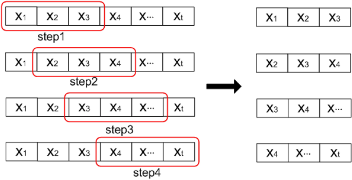
Process of sequence transformation from univariable to multivariable
-
Step 3: The last sequence is taken as the label set, and the first \(v\) sequence is taken as the training set; then:
$$\begin{gathered} S_{T} = \begin{array}{*{20}c} {\{ \{ x_{1} ,x_{2} ,...,x_{t - sv} \}^{T} ,\{ x_{s + 1} ,x_{s + 2} ,...,x_{t - s(v - 1)} \}^{T} } \\ {...,\{ x_{(v - 1)s + 1} ,x_{(v - 1)s + 2} ,...,x_{t - s} \}^{T} \} } \\ \end{array} \hfill \\ L_{T} = \{ x_{vs + 1} ,x_{vs + 2} ,...,x_{t} \}^{T} \hfill \\ \end{gathered}$$(10)where \(S_{T}\) is the training set, \(L_{T}\) is the label set, and the length of both sets is \((t - sv)\), forming the training model (TM) shown in the upper half of Fig. 6. This model can be expressed as:
$${\text{TM}} = F_{lstm} (S_{T} ,L_{T} ,(s,v))$$(11)

In (11), \(F_{lstm}\) represents the calculation method of the LSTM model (4–9), and \((s,v)\) represent constant variables, which are the length of the predicted data and the number of variables, respectively.
The LSTM model is reconstructed into a neural network (SL-LSTM) under a supervised learning mode through the multivariable processing of a single variable. The mathematical model is:
\(\tilde{X}\) represents the target data to be predicted and maintains the continuity of the time series with the single-variable sequence \(X\). In this paper, \(L_{T}\) is added to the end of \(S_{T}\), and the first variable in \(S_{T}\) is removed to form a new sample set \(S_{P}\) to maintain consistency in the number of variables, update the training set, and ensure the partial overlap and continuity of the data between variables.
The prediction model (PM) is shown in the bottom half of Fig. 6. The figure shows that the training set conversion from the TM to the PM is essentially a horizontal substitution between variables (the black arrows shown in Fig. 6). Finally, the TM is used to introduce the new sample set \(S_{P}\) and output the prediction set \(L_{P}\), so the PM can be expressed as:
In the output \(L_{P} = \{ x_{(v + 1)s + 1} ,x_{(v + 1)s + 2} ,...,x_{t} ,x_{t + 1.} ..,x_{n} \}\) of (13), \(\{ x_{(v + 1)s + 1} ,x_{(v + 1)s + 2} ,...,x_{t} \}\) is the fitting of known data, and \(\{ x_{t + 1.} ..,x_{n} \}\) is the prediction of unknown data.
Parameter selection optimization
The method we presented is a model based on the basic principles of LSTM. The reasonable selection of parameters directly affects the accuracy of model prediction. The general practice of setting the hyperparameters of neural network models is to use multiple experiments to obtain the optimal value, which is not repeated. The key parameter we discuss and analyze is the number of variables \(v\). The single-variable sequence is converted into a multivariable sequence for the purpose of expressing the nonlinear characteristics of the single difference sequence of clock bias as accurately as possible. Theoretically, the larger the \(v\) is, the higher the accuracy, but the lower the computational efficiency. Therefore, the selection of the value of \(v\) should consider the tradeoff between accuracy and computational efficiency. The following takes the G-03 satellite as an example for analysis and illustration.
The G-03 satellite data from October 1 to December 14, 2019, has a total of 21,600 sampling points in the 5 min sampling interval of precision clock bias, and the corresponding single difference sequence has 21,599 sampling points. The first 21,099 sampling points are used as training data, and the last 500 sampling points are used as the real values of the predicted data for comparative analysis. To analyze the optimal value of \(v\), we select a value within the interval of \(v \in [3,20]\) to conduct experiments through traversal. For the same hyperparameters, the root-mean-square error (RMSE) of the predicted and true values is calculated for different values of \(v\).
Figure 8 shows a comparison between the predicted data and the real data of the G-03 satellite for \(v = 3,7,14,20\). The solid black line in the figure represents the real data, and the solid red line represents the predicted data. The top-left panel shows the comparison results for \(v = 3\). In the figure, the fluctuation range of the predicted data is small, and the fitting degree of the periodic fluctuations of the real data is low. The top-right panel shows the comparison results for \(v = 7\). The fluctuation amplitude of the predicted data in the figure is significantly larger than that in the top-left panel, but the degree of fitting of the periodic fluctuation characteristics is still low. The bottom-left panel shows the comparison results for \(v = 14\). As shown in this figure, the predicted data exhibit an obvious fluctuation range and a high degree of fitting to the characteristics of the periodic fluctuations, and the fit is basically consistent with the fluctuation trend in the real data. The bottom-right panel shows the comparison results for \(v = 20\). The fluctuation amplitude and the degree of fitting of the periodic fluctuation characteristics of the predicted data shown in the figure are not much different from those shown in the bottom-left panel. This finding shows that the accuracy of the predicted values increases with an increasing \(v\) but decreases when \(v\) reaches a certain critical value.

Prediction results of satellite G-03 by the SL-LSTM model for different numbers of variables (top left: v = 3, top right: v = 7, bottom left: v = 14, and bottom right: v = 20). The solid black line is the G-03 clock difference, and the solid red line is the prediction results
Figure 9 shows the variation rule of the RMSE for the predicted and true values from \(v = 3\) to \(v = 20\). As shown in the figure, with a continuous increase in the value of \(v\), the RMSE continually decreases, indicating that the error between the predicted and real values continually decreases; that is, the accuracy of the predicted values continually improves. However, at \(v = 14\), the convergence trend in the RMSE is obvious, and with further increases in value, the decreasing trend in the RMSE further slows; this finding indicates that at \(v = 14\), the accuracy of the predicted values is close to optimal, and further increases in the value of \(v\) produce limited improvement in the accuracy of the predicted values. Considering the influence of the calculation efficiency, \(v = 14\) was determined to be the best value for the G-03 satellite data. To maintain the same experimental environment, in the following experiments, \(v = 14\) is used as the optimal value for different satellites.

RMSE values of the prediction results as a function of the \(v\) values
Experiments and analysis
The GPS data from October 1 to December 14, 2019, with a 5 min sampling interval precision clock bias provided by the IGS data center were used for experiments. Due to missing data from some satellites, only 21 satellites with good continuity were used for the experiments to ensure data continuity. (3) was used to address the problem of gross errors in the SCB. The experimental platform we used was based on Google's second-generation deep learning framework TensorFlow (1.0), and a rich model library on GitHub was used to build the experimental platform.
Clock bias prediction can generally be divided into short-, medium- and long-term predictions. To further evaluate the quality of SL-LSTM clock bias prediction, we conduct clock bias prediction for 3 h (h), 6 h, 12 h, 1 day (d), and 3 d. The experimental data are divided into training and prediction sets. Table 1 shows the basic situation of the experimental data. The 5 min sampling interval data are adopted, and the corresponding numbers of data points in the five forecasted time length sets are 36 (3 h), 72 (6 h), 144 (12 h), 288 (1 d), and 864 (3 d). Through many experiments, the network training parameters of the SL-LSTM model are determined as follows: the number of input nodes/number of variables (14), batch size (100), and training rounds (4000). To maintain the consistency in the experimental environment, we used the SL-LSTM method in the prediction experiments.
Example 1
Taking satellites G-03 and G-16 as examples, we adopt a wavelet neural network (WNN) with a two-layer feed-forward architecture, and the number of neurons in the hidden layer and the output are 6 and 1, respectively. We also adopted the ARIMA, QP, and SL-LSTM methods to conduct prediction experiments, used the RMSE and mean of the predicted and true values to evaluate the prediction accuracy of the algorithms, and used the absolute value of the difference between the maximum and minimum errors (range) to evaluate the stability of the algorithms.
To comprehensively evaluate the effect of the SL-LSTM method under different prediction time conditions, five time durations of 3 h, 6 h, 12 h, 1 d, and 3 d were predicted. Figure 10 shows the error results between the predicted values of satellites G-03 (top) and G-16 (bottom) and the true values. In the figure, the solid red line represents the prediction results of the SL-LSTM method, the solid purple line represents the prediction results of the WNN method, the solid blue line represents the prediction results of the ARIMA method, and the solid green line represents the prediction results of the QP method. Tables 2, 3, 4 show the calculated RMSE, mean, and range, respectively, of the satellite prediction results for G-03 and G-16.

Comparison of the prediction errors for 3 h (top left), 6 h (top middle), 12 h (top right), 1 d (bottom left), and 3 d (bottom right) for G-03 and G-16 based on the WNN, ARIMA, QP, and SL-LSTM methods
Compared with the other three methods, the SL-LSTM method has no obvious advantages in the prediction results for the G-03 and G-16 satellites for 3 h (Fig. 10 (top left)) of clock bias prediction, and its accuracy and stability are slightly lower than those of the WNN method (Tables 2, 3, 4). The same problem exists in the predictions for 6 h (top center) and 12 h (top right) of clock bias prediction. This finding suggests that the SL-LSTM method does not have obvious advantages over the other three methods for short-term prediction. In particular, the prediction accuracy of the WNN method is superior to that of the SL-LSTM method for the 3 h duration and only slightly lower than that of the SL-LSTM method for the 6 h duration, and the error in the cumulative speed is small. The error in the ARIMA method accumulates quickly with increasing prediction time.
In the clock bias prediction for 1 d and 3 d (Fig. 10 (bottom left and bottom right, respectively)), the accuracy of the SL-LSTM method is obviously better than that of the other three methods, the error divergence degree is low, and the trend is stable; in contrast, the error divergence rates of the other three methods are significantly accelerated. The RMSE (10–11 s) of the SL-LSTM method was 5.2366 under the conditions of a 3 h duration of the G-03 satellite, and the RMSE (10–11 s) was 62.5409 under the conditions of a 3 d duration, which is an increase of 10.94-fold ((62.5409–5.2366)/5.2366 = 10.94). The increase for the G-16 satellite was 5.39-fold. Those values for the WNN method increased by 28.17-fold and 12.27-fold, those for the ARIMA method increased by 606.45-fold and 23.41-fold, and those for the QP method increased by 4.45-fold and 1.2-fold, respectively. Although the error divergence is low, the RMSE is large. Further analysis of the variation in the mean and range values also reflects the above characteristics.
These results suggest that for the G-03 and G-16 satellites, the SL-LSTM long-term prediction accuracy is superior to those of the other three methods. As the prediction time increases, the error accumulation rate is lower than those of the other three methods, and this method embodies good stability. For short-term prediction, compared with the other three methods, our method exhibits no significant advantages, and a more comprehensive evaluation of all the available SCB prediction results is needed.
Example 2
To further comprehensively evaluate the predictive ability of the SL-LSTM method, we deal with all 21 available SCB prediction experiments. The parameter set is consistent with that in example 1. The RMSE and mean of predicted and true values are used to evaluate the prediction accuracy of the algorithm. The absolute value of the difference between the maximum and minimum errors (range) is used to evaluate the stability of the algorithm.
In example 1, from the perspective of the satellites, we analyzed and evaluated the predictive ability of the WNN, ARIMA, QP, and SL-LSTM methods for the G-03 and G-16 satellites under the conditions of 3 h, 6 h, 12 h, 1 d, and 3 d. In example 2, from the perspective of the methods, we analyze and evaluate their predictive ability for the 21 available satellites under the conditions of 3 h, 6 h, 12 h, 1 d and 3 d. Figure 11 presents the clock bias prediction errors for the five durations. For the predicted result statistics, Table 5 shows the \(\overline{RMSE}\), \(\overline{Mean},\) and \(\overline{Range}\) for the 21 available satellite prediction results, representing the average RMSE, average mean, and average range, respectively. The mathematical expressions are:

Comparison of the prediction errors for 3 h (top left), 6 h (top middle), 12 h (top right), 1 d (bottom left), and 3 d (bottom right) for the available satellites based on the WNN, ARIMA, QP, and SL-LSTM methods
In (14) to (16), \(n = 21\). Figure 11 shows the prediction results of the available satellites for 3 h (upper left), 6 h (upper center), 12 h (upper right), 1 d (lower left), and 3 d (lower right) by using the WNN, ARIMA, QP, and SL-LSTM methods. In the top-left panel, the distribution of the QP method's prediction error (solid green line) was relatively scattered, while other methods were relatively concentrated at approximately 0, indicating that the prediction error of the QP method was lower than that of the other methods at a duration of 3 h. With increasing duration, the prediction error of different methods changed substantially. The ARIMA method (solid blue line) diverged faster than the other methods, indicating that the stability was not good. The divergence speed of the WNN method (solid purple line) was slightly higher than that of the SL-LSTM method. From the qualitative analysis, the SL-LSTM method was superior to the other methods in terms of the prediction quality. By combining the statistical analysis of the clock bias prediction results shown in Table 5, it can be seen that the accuracy advantage of the SL-LSTM clock bias prediction is not obvious for short-term prediction, especially the prediction results for 3 h and 6 h. In units of 10–11 s and prediction duration of 3 h, the value for the SL-LSTM method is 32.8861, which is slightly greater than that of the WNN of 27.1457, and significantly smaller than 53.2328 and 186.5904 obtained for the ARIMA and QP, respectively. For the 6 h prediction duration, the value for the SL-LSTM method is 45.7252, which is slightly greater than that for the WNN (44.8904) and significantly smaller than the ARIMA and QP values of 132.4619 and 189.6142, respectively. Similarly, the results of the SL-LSTM method for \(\overline{Mean}\) are basically the same as those for \(\overline{RMSE}\), indicating that the SL-LSTM method has no obvious advantage in short-term prediction accuracy over the WNN, but this method is still better than the ARIMA and QP. The SL-LSTM method also has no obvious advantage in evaluating the \(\overline{Range}\) value, indicating the stability of the predicted results.
With an increase in the prediction time, the accuracy of the SL-LSTM method remains at a high level and is obviously better than those of the other methods. Particularly for the 3 d prediction duration, the \(\overline{RMSE}\) in units of 10–11 s for the SL-LSTM is 159.9000, which is obviously less than 270.0857 achieved for the WNN (270.0857) and significantly less than 2915.6619 and 382.7952 for the ARIMA and QP, respectively. Similarly, the results of the SL-LSTM for \(\overline{Mean}\) are basically consistent with those for \(\overline{RMSE}\), and this method has obvious advantages in evaluating the \(\overline{Range}\) value, which indicates the stability of the predicted results. These results show that the SL-LSTM method has a higher accuracy and stability in long-term prediction than the WNN, ARIMA, and QP methods.
Based on Table 5, it can be seen that, in terms of the precision and stability of the prediction results (RMSE), the proposed SL-LSTM method outperforms the other models in the five prediction durations (3 h, 6 h, 12 h, 1 d, and 3 d) for most GPS satellite clock types. Specifically, compared with the results of the WNN method, the average prediction RMSE of the SL-LSTM method improved by approximately −21.80, −1.85, 8.57, 2.27, and 40.79% compared with the results of the ARIMA method. The average prediction RMSE of the SL-LSTM method improved by approximately 38.23, 65.48, 80.22, 85.18 and 94.51% compared with the results of the QP method, and the average prediction RMSE of the SL-LSTM method improved by approximately 82.37, 75.88, 67.24, 45.71 and 58.22%.
Figure 12 shows the clock bias prediction trend variation, where the horizontal axis is the prediction time length (period), and the vertical ordinate values in panels (a–c) present the \(\overline{RMSE}\), \(\overline{Mean},\) and \(\overline{Range}\) values, respectively. The SL-LSTM method can be used to predict the results of changes in the \(\overline{RMSE}\), \(\overline{Mean},\) and \(\overline{Range}\) values with the prediction time minimum amplitude. The SL-LSTM method has better accuracy and stability than the other three methods, especially compared with the ARIMA method (blue line). There is a small gap between the WNN method (purple line) and the SL-LSTM method, which indicates that the neural network has significant advantages in clock bias prediction, but the accuracy of the WNN predictions increases significantly with a continuous increase in the prediction duration. The prediction accuracy of the QP method is lower than those of the SL-LSTM and WNN methods. In addition, under the same experimental conditions, a 3 d prediction duration is taken as an example. For the WNN method, the whole process takes < 5 min, while the SL-LSTM method takes < 3 min, indicating that the time complexity of the SL-LSTM method is less than that of the WNN method, and the SL-LSTM method is better than the WNN method.

Comparison of the SCB prediction results
Conclusion
Using the single difference sequence of clock bias as the research object and an improved MAD method after eliminating gross error data, we propose a SL-LSTM network model based on an LSTM network and the basic principles of supervised learning. Our model is based on the single difference sequence of cyclic and random feature modeling and realization of the clock bias prediction function. We show that the SL-LSTM method can further improve clock bias prediction accuracy and stability through experimental comparison and analysis. In summary, our method has the following advantages:
-
(1) The prediction errors of traditional clock bias prediction methods represented by the ARIMA and QP methods increase rapidly with an increase in the prediction time, while the SL-LSTM method has a significant advantage in controlling the accumulation of the prediction errors with the prediction time and is more suitable for medium- and long-term prediction.
-
(2) The proposed method has a high degree of reduction in the cyclic and random features of the clock bias, which is the key to further improving the prediction accuracy.
-
(3) An LSTM network is an effective tool for dealing with time series data. Addressing a typical time series data processing problem, we improve an LSTM network to realize the effective application of clock bias prediction and achieve good results, and this work makes a beneficial attempt to further study the problem of clock bias prediction.
There are still some aspects of the method presented in this paper that need further study and improvement:
-
(1) The proposed method needs to be further studied in terms of short-term clock prediction accuracy and stability.
-
(2) The proposed method needs to be studied further for the training method of parameter selection optimization to further enhance the practical value of this method.
Data availability
We thank the IGS Data Center of Wuhan University for providing open source data for this study. The website is http://www.igs.gnsswhu.cn/index.php/Home/DataProduct/igs.html
Abbreviations
- ANN:
-
Artificial neural network
- ARIMA:
-
Autoregressive integrated moving average
- GM:
-
Grey model
- GNSS:
-
Global navigation satellite system
- IGS:
-
International GNSS Service
- KF:
-
Kalman filtering
- LSTM:
-
Long short-term memory
- MAD:
-
Median absolute deviation
- QP:
-
Quadratic polynomial
- RNN:
-
Recurrent neural network
- SA:
-
Spectrum analysis
- SCB:
-
Satellite clock bias
- SL-LSTM:
-
Supervised learning long short-term memory
- WNN:
-
Wavelet neural network
References
Ai QS, Xu TH, Li JJ, Xiong HW (2016) The short-term forecast of BeiDou satellite clock bias based on wavelet neural network. China Satellite navigation conference (CSNC) 2016 proceedings: Volume I, pp 145–154
Cui XQ, Jiao WH (2005) Grey system model for the satellite clock error predicting. Geomat Inf Sci Wuhan Univ 30(5):447–450
Davis J, Bhattarai S, Ziebart M (2012) Development of a Kalman filter based GPS satellite clock time-offset prediction algorithm. European frequency and time forum, proceedings: pp 152–156
Donahue J, Hendricks LA, Rohrbach M, Guadarrama S (2015) Long-term recurrent convolutional networks for visual recognition and description. IEEE Trans Pattern Anal Mach Intell 39(4):677–691
Greff K, Srivastava RK, Koutnik J, Steunebrink BR, Schmidhuber J (2016) LSTM: a search space odyssey. IEEE Trans Neural Netw Learn Syst 28(10):2222–2232
Hao X, Du Q, Reynolds M (2018) SS-LSTM: A hierarchical LSTM model for pedestrian trajectory prediction. 2018 IEEE winter conference on applications of computer vision (WACV), Lake Tahoe, NV, pp. 1186–1194
Heo YJ, Cho J, Heo MB (2010) Improving prediction accuracy of GPS satellite clocks with periodic variation behaviour. Meas Sci Technol 21(7):073001
Hochreiter S, Schmidhuber J (1997) Long short-term memory. Neural Comput 9(8):1735–1780
Huang BH, Yang BH, Li MG, Guo ZK, Mao JY, Wang H (2021) An improved method for MAD gross error detection of clock error. Geomatics and information science of Wuhan University (accepted for publication)
Huang GW, Cui BB, Zhang Q, Fu WJ (2018) Real-time clock offset prediction model with periodic and neural network corrections. J Astronaut 39(1):83–88
Huang G, Yang Y, Zhang Q (2011) Estimate and predict satellite clock error using adaptively robust sequential adjustment with classified adaptive factors based on opening windows. Acta Geodaetica Et Cartographica Sinica 40(1):15–21
Huang G, Zhang Q (2012) Real-time estimation of satellite clock offset using adaptively robust Kalman filter with classified adaptive factors. GPS Solut 16(4):531–539
Huang GW, Zhang Q, Xu GC (2014) Real-time clock offset prediction with an improved model. GPS Solut 18(1):95–104
Lecun Y, Bengio Y, Hinton G (2015) Deep learning. Nature 521(7553):436–444
Lei Y, Zhao DN (2014) The satellite clock bias forecast based on empirical mode decomposition and least squares support vector machines. Acta Astronom Sinica 55(3):216–227
Liang YJ, Ren C, Yang XF, Peng GF, Lan L (2015) Grey model based on first difference in the application of the satellite clock bias prediction. Acta Astronom Sinica 56(3):264–277
Lu XF, Yang ZQ, Jia XL, Cui XQ (2008) Parameter optimization method of gray system theory for the satellite clock error predicating. Geomat Inform Sci Wuhan Univ 33(5):492–495
Wang GC, Liu LT, Xu AG, Su XQ, Liang XH (2014) The application of radial basis function neural network in the GPS satellite clock bias prediction. Acta Geodaetica Et Cartographica Sinica 43(8):803–807
Wang X, Wu J, Liu C, Yang HY, Du YL, Niu WS (2018) Exploring LSTM based recurrent neural network for failure time series prediction. J Beijing Univ Aeronaut Astronaut 44(4):772–784
Wang YP, Lu ZP, Qu YY, Li LY, Wang N (2016a) Improving prediction performance of GPS satellite clock bias based on wavelet neural network. GPS Solut 21(2):1–12
Wang YP, Lu ZP, Sun DS, Wang N (2016b) A new navigation satellite clock bias prediction method based on modified clock-bias quadratic polynomial model. Acta Astronom Sinica 57(1):78–90
Wang YP, Lu ZP, Zhou HT, Wang N, Zhai SF (2016c) Satellite clock bias prediction based on modified single difference data of clock bias. J Geodesy Geodyns 36(12):1073–1077
Xu C, Li B, Liu JL, Wu HB, Hu YH (2017) A modified method for clock error simulation of high precision frequency source. J Astronaut 38(9):998–1004
Xu JY, Zeng AM (2009) Application of ARIMA(0,2, q) model to prediction of satellite clock error. J Geodesy Geodyn 29(5):116–120
Vinyals O, Toshev A, Bengio S, Erhan D (2015) Show and tell: a neural image caption generator. IEEE conference on computer vision and pattern recognition. Piscataway, NJ: IEEE Press: 3156–3164
Zhao L, Lan XQ, Sheng JY (2012) Application of ARIMA model in satellite clock error forecasting. J Water Resour Archit Eng 10(1):135–137
Zheng ZY, Dang YM, Lu XS, Xu WM (2010) Prediction model with periodic item and its application to the prediction of GPS satellite clock bias. Acta Astronom Sinica 51(1):95–102
Acknowledgments
This study has been supported by the National Natural Science Foundation of China (61973328).
Author information
Authors and Affiliations
Corresponding author
Additional information
Publisher's Note
Springer Nature remains neutral with regard to jurisdictional claims in published maps and institutional affiliations.
Rights and permissions
Open Access This article is licensed under a Creative Commons Attribution 4.0 International License, which permits use, sharing, adaptation, distribution and reproduction in any medium or format, as long as you give appropriate credit to the original author(s) and the source, provide a link to the Creative Commons licence, and indicate if changes were made. The images or other third party material in this article are included in the article's Creative Commons licence, unless indicated otherwise in a credit line to the material. If material is not included in the article's Creative Commons licence and your intended use is not permitted by statutory regulation or exceeds the permitted use, you will need to obtain permission directly from the copyright holder. To view a copy of this licence, visit http://creativecommons.org/licenses/by/4.0/.
About this article

Cite this article
Huang, B., Ji, Z., Zhai, R. et al. Clock bias prediction algorithm for navigation satellites based on a supervised learning long short-term memory neural network. GPS Solut 25, 80 (2021). https://doi.org/10.1007/s10291-021-01115-0
Received:
Accepted:
Published:
DOI: https://doi.org/10.1007/s10291-021-01115-0