Parallel and distributed computing for stochastic dual dynamic programming

Abstract

We study different parallelization schemes for the stochastic dual dynamic programming (SDDP) algorithm. We propose a taxonomy for these parallel algorithms, which is based on the concept of parallelizing by scenario and parallelizing by node of the underlying stochastic process. We develop a synchronous and asynchronous version for each configuration. The parallelization strategy in the parallelscenario configuration aims at parallelizing the Monte Carlo sampling procedure in the forward pass of the SDDP algorithm, and thus generates a large number of supporting hyperplanes in parallel. On the other hand, the parallel-node strategy aims at building a single hyperplane of the dynamic programming value function in parallel. The considered algorithms are implemented using Julia and JuMP on a high performance computing cluster. We study the effectiveness of the methods in terms of achieving tight optimality gaps, as well as the scalability properties of the algorithms with respect to an increasing number of CPUs. In particular, we study the effects of the different parallelization strategies on performance when increasing the number of Monte Carlo samples in the forward pass, and demonstrate through numerical experiments that such an increase may be harmful. Our results indicate that a parallel-node strategy presents certain benefits as compared to a parallel-scenario configuration.

1 Introduction

The stochastic dual dynamic programming (SDDP) algorithm, developed by Pereira and Pinto (1991), has emerged as a scalable approximation method for tackling multistage stochastic programming problems. The algorithm is based on building piecewise linear approximations of the value functions of the dynamic programming equations. The algorithm has its origins in hydrothermal scheduling (Pereira and Pinto, 1991; Flach et al., 2010; De Matos et al., 2010; Pinto et al., 2013), although other applications have emerged in recent years, including day-ahead bidding of pumped-hydro storage plants (Löhndorf et al., 2013), natural gas storage valuation (Löhndorf and Wozabal, 2020), dairy farm operations (Dowson et al., 2019), and short-term energy dispatch (Papavasiliou et al., 2017; Kaneda et al., 2018).

Multistage stochastic programming problems are generally computationally intractable and therefore pose serious computational challenges, even for SDDP. For example, SDDP is unable to close the optimality gap for the problem studied in Shapiro et al. (2013), even after several hours of run time. In order to reduce the complexity of the algorithm, different techniques have been proposed in the literature. With an objective of limiting the complexity of the cost-to-go function, cut selection techniques are considered in De Matos et al. (2015); Guigues (2017); Guigues and Bandarra (2019); Löhndorf et al. (2013).

Regularization techniques are studied in Asamov and Powell (2018) in order to accelerate convergence.

The nature of the SDDP algorithm makes it suitable for parallel computing (Pereira and Pinto, 1991). This has led to parallel schemes for SDDP in past research that aim at improving the performance of the algorithm (da Silva and Finardi, 2003; Pinto et al., 2013; Helseth and Braaten, 2015; Dowson and Kapelevich, 2021; Machado et al., 2021).

1.1 Parallelism in large-scale optimization

Parallelism is a crucial attribute for tackling large-scale optimization problems, but is often undermined by synchronization bottlenecks. In power system applications, for instance, parallelism has allowed tackling large-scale day-ahead stochastic unit commitment problems (Papavasiliou et al., 2014). While synchronous parallel computing algorithms require run times in the order of a weeks for certain instances of stochastic unit commitment, asynchronous implementations of Lagrange relaxation have been shown to reduce these run times to a few hours (Aravena and Papavasiliou, 2020). This allows us to hope for an eventual deployment of stochastic operational planning models in actual operations, where run time constraints are critical.

This objective motivates our research on the parallelism attributes of SDDP. Nevertheless, the extant literature on SDDP presents a limited study in this front. The literature provides a narrow set of parallel schemes, which rely on increasing the number of Monte Carlo samples that are used in the forward pass of the algorithm (da Silva and Finardi, 2003; Pinto et al., 2013; Helseth and Braaten, 2015; Dowson and Kapelevich, 2021). The aforementioned literature provides evidence that such schemes are superior relative to a serial approach. The literature, however, does not focus on how different schemes may compare relative to each other.

In Pinto et al. (2013) and da Silva and Finardi (2003) the authors propose a synchronous parallel scheme, according to which subproblems are solved in parallel at every stage. Parallelization is also applied in the backward pass of the algorithm. This introduces a natural synchronization bottleneck at each stage. In Helseth and Braaten (2015) the authors propose a relaxation in the synchronization points of this synchronous parallel scheme. According to the proposed scheme, a worker waits for a subset of subproblems at each stage of the backward pass. The authors provide empirical evidence that demonstrate that their approach achieves performance gains relative to the synchronous setting. However, the analysis is not sufficiently robust, since the authors declare convergence once the lower bound is within the 95% confidence interval of the upper bound. This convergence criterion has been criticized in Shapiro (2011).

In our work, we propose a richer family of parallelizable algorithms for SDDP. Our analysis considers synchronous as well as asynchronous computation. We develop a taxonomy of (i) parallelization by scenario of Monte-Carlo samples in the forward pass of the algorithm, and (ii) parallelization by node of the underlying stochastic process, that encompasses the traditional parallel schemes that are encountered in the literature, and gives rise to new parallel formulations. We present an analysis for the resulting class of algorithms, and compare the relative strengths and weaknesses of the proposed algorithms.

1.2 Limitations of parallelism

Parallelism is often viewed as a one-way procedure, where more processors necessarily imply better performance. The SDDP literature tends to consider an increase in the number of Monte Carlo samples in the forward pass, in order to be able to rely on more processors (da Silva and Finardi, 2003; Pinto et al., 2013; Helseth and Braaten, 2015; Dowson and Kapelevich, 2021). Nevertheless, there is a lack of evidence for assessing the effect of such an increase on the performance of the SDDP algorithm. In our work, we present empirical evidence which indicates that increasing the number of Monte Carlo samples in the forward pass of the SDDP algorithm may in fact undermine performance. This indicates a serious drawback with traditional parallel schemes that have been proposed in the literature, since it indicates that these traditional parallel schemes may not scale well.

1.3 Contributions

Our contribution to the literature on SDDP parallelization is two-fold. First, we enrich the set of available parallel schemes that have been considered in the literature, by considering both synchronous as well as asynchronous computation, and we present a taxonomy that categorises existing and new schemes. Second, we conduct an extensive numerical experiment in order to compare the relative performance of these schemes when the objective is to achieve tight optimality gaps with high confidence. Moreover, our analysis provides empirical evidence that indicates that increasing the number of parallel processors may harm the performance of traditional parallel schemes that have been proposed for SDDP.

The paper is organized as follows. In Sect. 2 we present the notation and formulation of Multistage Stochastic Programs, and we describe the SDDP algorithm. In Sect. 3 we describe our proposed parallelization schemes for SDDP. In Sect. 4 we present numerical case studies which constitute the basis for our empirical observations. Finally, in Sect. 5 we summarize our conclusions and outline future directions of research that are inspired by this work.

2 Stochastic dual dynamic programming (SDDP)

Let us consider a multistage stochastic linear program with T stages, given by

$$ \min_{\substack{ A_{1} x_{1} = b_{1} \\ x_{1} \ge 0 } } c_{1}^{T} x_{1} + {\mathbb{E}}[\min_{\substack{ B_{2} x_{1} + A_{2} x_{2} = b_{2} \\ x_{2} \ge 0 } } c_{2}^{T} x_{2} + {\mathbb{E}}[ \cdots + {\mathbb{E}}[\min_{\substack{ B_{T} x_{T - 1} + A_{T} x_{T} = b_{T} \\ x_{T} \ge 0 } } c_{T}^{T} x_{T} ]]] $$

Here, the vectors c_t,b_t as well as the matrices B_t,A_t form the stochastic data process ξ_t = (c_t,b_t,B_t,A_t). We assume that c₁,b₁,A₁ are deterministic. Let us assume that, at each stage, there are finitely many outcomes Ω_t, and that the data process follows a Markov chain. The dynamic programming equations can be written as

$$ \begin{aligned} & Q_{t} (x_{t - 1} ,\xi_{t} ) = \min_{{x_{t} }} \{ c_{t}^{T} x_{t} + {\mathcal{Q}}_{t + 1} (x_{t} ,\xi_{t} ):B_{t} x_{t - 1} + A_{t} x_{t} = b_{t} ,x_{t} \ge 0\} \\ & {\mathcal{Q}}_{t + 1} (x_{t} ,\xi_{t} ): = {\mathbb{E}}[Q_{t + 1} (x_{t} ,\xi_{t + 1} )|\xi_{t} ] \\ \end{aligned} $$

for t = 2,···,T. There is no associated function ${\mathcal{Q}}_{T + 1}$ in the last stage. Note that, due to the Markov property, the cost-to-go function $Q_{t} (x_{t - 1} ,\xi_{t} )$ and the expected value cost-to-go functions ${\mathcal{Q}}_{t + 1} (x_{t} ,\xi_{t} )$ depend only on ξ_t, and not on the entire history of the data process. Moreover ${\mathcal{Q}}_{t + 1} (x_{t} ,\xi_{t} )$ is a convex function of x_t (Birge and Louveaux, 2011) and can therefore be approximated by a piecewise linear function. The idea of SDDP is to generate approximations $\widehat{{\mathcal{Q}}}_{t + 1} (x_{t} ,\xi_{t} )$ of the expected value cost-to-go functions through supporting hyperplanes H, commonly referred to as cuts. The cost-to-go functions can then be approximated as:

$$ \hat{Q}_{t} (x_{t - 1} ,\xi_{t} ) = \min_{{x_{t} }} \{ c_{t}^{T} x_{t} + \widehat{{\mathcal{Q}}}_{t + 1} (x_{t} ,\xi_{t} ):B_{t} x_{t - 1} + A_{t} x_{t} = b_{t} ,x_{t} \ge 0\} $$

The procedure for generating a cut H is a two-step process that consists of forward and backward passes. During forward passes, we generate trial points. During backward passes, we generate cuts for the expected value cost-to-go functions at the trial points.

• 1. Forward Pass Draw N Monte Carlo scenarios of the realization of uncertainty throughout the entire time horizon of the problem. This yields sequences $\xi_{1}^{n} , \cdots ,\xi_{T}^{n}$, where $\xi_{t}^{n} \in \Omega_{t}$ for n = 1,···,N.

  

This process produces trial points $\hat{x}_{1}^{n} , \cdots ,\hat{x}_{T}^{n}$ for n = 1,···,N.

• 2. Backward Pass

  

This two-step process constitutes an iteration of the algorithm. In Philpott and Guan (2008) it is proven that this procedure converges, meaning that the algorithm converges almost surely after finitely many iterations.

A common and attractive way to represent this process and the underlying structure of the problem graphically, relies on a lattice representation of uncertainty. Figure 1 presents a lattice, where each column represents a time stage of the problem, and where each node represents the possible outcomes at the current time stage. Note that each node of the lattice is associated with an optimization problem, which aims at minimizing the current-period cost plus the cost-to-go function of the given node.

Fig. 1

Lattice representation of uncertainty in SDDP. Each node corresponds to a realization of uncertainty. Nodes grouped in the same column correspond to a given time stage of the problem. Lines connecting nodes represent the probability of transitioning form one node to another. Each node stores an associated subproblem and a value function

Figure 2 presents an SDDP iteration graphically over a lattice. The computational time evolves along the y axis, as indicated by the left-most arrow. The red dashed boxes indicate the work that a CPU is performing over the lattice and the y axis length represents the elapsed computational time for the current task. During a forward pass, a sample path is drawn from the distribution implied by the lattice. This results in selecting the red nodes in the figure, namely nodes 1, 2, and 5. The subproblems associated to these nodes are solved, starting from the first stage to the last one, that is node 1, then node 2, and finally node 5. This process produces trial points $\hat{x}_{1} , \cdots ,\hat{x}_{T}$. Note that the subproblems at each stage are calculated at the trial point that is obtained in the previous time stage. The backward pass procedure moves backward in time, starting from the last stage and moving towards the first stage. At the last stage, the subproblems associated to nodes 7, 6, and 5 are solved at the trial point $\hat{x}_{2}$. The order in which these nodes are solved is not critical. The dual multipliers of these problems are used for computing a cut of the value functions of stage 2 at point $\hat{x}_{2}$. The procedure continues in this manner throughout all stages.

Fig. 2

Graphical representation of the SDDP algorithm on a lattice. The position of the red dashed boxes on the y axis represents the elapsed computational time. The forward pass draws a sample path and produces trial points $\hat{x}_{1} ,\hat{x}_{2}$. During the backward pass, the third stage produces a cut at $\hat{x}_{2}$ for the value functions associated to nodes in stage 2. The second stage generates a cut at $\hat{x}_{1}$ for the value functions associated to nodes in stage 1

3 Parallel schemes for SDDP

We begin this section by presenting parallel strategies for SDDP and then proceed to explain how these strategies can be implemented in a synchronous and asynchronous setting. These schemes span the different strategies that have been proposed in the literature (da Silva and Finardi, 2003; Pinto et al., 2013; Helseth and Braaten, 2015; Dowson and Kapelevich, 2021; Machado et al., 2021) and some new schemes that, to the best of our knowledge, have not yet been considered.

3.1 Parallelizing by scenario and by node

3.1.1 Parallelizing by scenario (PS)

As we demonstrate graphically in panel (a) of Fig. 3, in this approach, each processor generates a cut that supports the expected value cost-to-go functions at different sample points of the state space. The forward and backward steps are executed as follows:

• Forward pass The forward pass consists of N Monte Carlo scenarios. Each processor computes a different scenario, thus producing trial points $x_{1}^{n} , \cdots ,x_{T}^{n}$ in the state space, for n = 1,···,N.

• Backward pass At stage t, the nth processor generates a cut for the expected cost-to-go functions of stage t − 1 at point $x_{t - 1}^{n}$.

Fig. 3

Representation of SDDP parallel schemes. The height of the red and blue dashed boxes represents the elapsed time. a Presents the parallel scenario scheme. At each iteration a cut is built at 2 different points, and each cut is computed by a different CPU. b Presents the parallel node scheme. The grey dashed boxes represent outcomes that belong to the same time stage. At each iteration, a cut is computed at a single point of the state space. The work that is required for computing such a cut is distributed among the available CPUs

The Parallel Scenario approach appears to be the most common parallelization strategy for SDDP in the literature. Different variants have been proposed, ranging from synchronous schemes (da Silva and Finardi, 2003; Pinto et al., 2013) to relaxations in the synchronization points (Helseth and Braaten, 2015), to asynchronous schemes (Dowson and Kapelevich, 2021).

3.1.2 Parallelizing by node (PN)

In panel (b) of Fig. 3 we can observe that, as opposed to the PS strategy, the idea in PN strategies is to use the available processors in order to generate a single cut at a single trial point. The forward and backward steps are executed as follows:

• Forward Pass The main processor computes trial points along a single scenario. This produces a sequence $x_{1} , \cdots x_{T}$. Note that there is no parallelization at this step.

• Backward Pass Moving backwards in time through the lattice, each processor selects a node of the lattice that has not yet been updated and solves the corresponding subproblem.

A competitive implementation for this scheme is unfortunately limited to a shared memory setting. This is due to the fact that, when a CPU commences a task in a distributed memory setting, there is a non-negligible communication startup time involved with receiving the required data for commencing the task. This implies that the task executed by each processor must require significantly more time than this start up time if parallelism is to deliver benefits, otherwise the latency of the network becomes an important factor in slowing down the algorithm. In the PN scheme, at stage t, each processor withdraws a subproblem from the list of |Ω_t| problems and proceeds to solve it. In a distributed memory setting, this solve time is comparable to the startup time of the processor. Thus, the latency of the network becomes problematic.

In Machado et al. (2021) a similar approach is followed, a single scenario is considered and the work required to compute the scenario is distributed among the workers. However, the authors consider a different scheme to distribute the nodes among the processors. They allow processors to be attached to a stage. The processors are then constantly generating cuts for the given stage.

3.2 Synchronous and asynchronous computing

As is commonly the case in parallel computing algorithms (Bertsekas and Tsitsiklis, 1989), the interaction between processors in our proposed schemes can unfold synchronously or asynchronously. In what follows, we propose synchronous and asynchronous schemes for both the parallel scenario (PS) and parallel node (PN) versions of SDDP. This leads to a variety of algorithms, which are summarized in Table 1.

Table 1 SDDP schemes compared in this paper

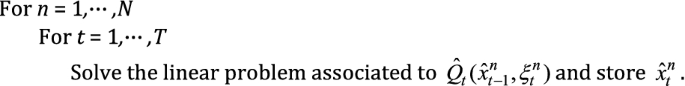
3.2.1 Synchronous parallel scenario (sync PS)

As we discuss in Sect. 3.1.1, in the PS scheme each processor builds a cut. The difference between the synchronous and asynchronous version of the algorithm is how these cuts are exchanged between processors. Given N processors, the forward and backward procedures for the synchronous PS scheme can be described as follows.

• 1. Forward Pass: The n-th processor computes a Monte Carlo scenario, thus obtaining a sequence $\xi_{1}^{n} , \cdots ,\xi_{T}^{n}$, where $\xi_{t}^{n} \in \Omega_{t}$.

  

  At the end of this step, the processors synchronize¹

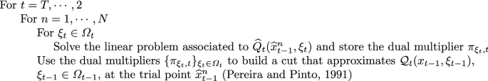
• 2. Backward Pass:

The n-th processor solves:

In panel (a) of Fig. 4 we present the evolution of the algorithm over a lattice. In the forward pass, the processors compute a scenario and synchronize at the end of the forward pass. In the backward pass, at stage 3, both processors compute a cut which is shared in order to approximate the expected value cost to go functions. Because of the synchronization, both processors must wait until receiving the cut of the other processor. If one processor is faster when computing a cut, then it must stay idle until all other processors have computed their cut. Note that, apart from the synchronization at the end of each stage during the backward pass, synchronization also occurs at the end of the backward pass. Consequently, in the next iteration, all processors commence with the same set of cuts.

Fig. 4

Synchronous and asynchronous parallel scenario schemes. The height of the red and blue dashed boxes represents the elapsed time

The synchronous version appears in a number of publications (da Silva and Finardi, 2003; Pinto et al., 2013). In Helseth and Braaten (2015) the authors propose a relaxation in the synchronization points of each stage of the backward pass, whereby a processor waits for a subset of processors. This work discusses empirical evidence that indicate benefits relative to a fully synchronous version.

3.2.2 Asynchronous parallel scenario (async PS)

The difference between Async PS and the synchronous version is that processors do not wait for cuts that have not been computed yet. The algorithm can be described as follows.

• 1. Forward pass: The n-th processor performs the same steps as in the synchronous setting, the difference is that there is no synchronization.

• 2. Backward pass:The n-th processor solves:

  

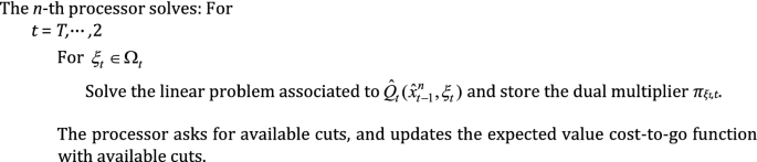
As we can observe in panel (b) of Fig. 4, in the forward pass each processor computes a sample and proceeds immediately to the backward pass. In the backward pass, once a processor computes a cut, this cut is shared with the master process. The processor then asks for available cuts and proceeds without waiting for cuts that have not been computed yet. For instance, at stage 3, the blue processor computes a cut faster than the red processor, sends the cut and asks if the cut provided by the red processor is already available. Since the red processor has not finished its job, the blue processor proceeds to stage 2 without waiting for the cut provided by the red processor. On the other hand, once the red processor finishes stage 3, it will receive the cut provided by the blue processor. A disadvantage of this scheme is that, since every processor operates with a different set of cuts, it is not clear how to estimate an upper bound. In Sect. 4 we discuss how the convergence evolution is measured.

In Dowson and Kapelevich (2021) the authors follow the aforementioned asynchronous strategy, nevertheless no evidence of its benefits are developed in detail.

3.2.3 Synchronous parallel node (sync PN)

In Sect. 3.1.2 we present the PN scheme, according to which different processors are allocated to different nodes of the lattice for a given stage. The synchronous and asynchronous schemes then differ on whether a processor waits for the nodes computed by other processors. The forward and backward passes can be described as follows.

• 1. Forward pass: The main process computes a single Monte Carlo scenario, thus obtaining a sequence $\xi_{1} , \cdots ,\xi_{T}$, where $\xi_{t} \in \Omega_{t}$.

  

Note that there is no parallelization in this step.

• 2. Backward Pass:

  

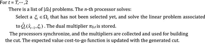
In Fig. 5, panel (a), we present this process graphically over a lattice. Note that, in stage 3, the blue processor solves the subproblem associated with the first node, while the red processor solves the subproblem associated with the second node. The red processor finishes first and proceeds with the third node. Note that, once the blue processor finishes, it must stay idle as there are no more nodes available for that stage. The solution information of all the nodes is then used in order to compute a cut, which is then transmitted to stage 2. Note that, before passing to stage 2, all the subproblems of the third stage must be solved.

Fig. 5

Synchronous and asynchronous parallel node schemes. The height of the red and blue dashed boxes represents the elapsed time. The dashed grey box represents outcomes that belong to the same stage

3.2.4 Asynchronous parallel node (async PN)

In contrast to the synchronous version, in the asynchronous version the processors do not wait for nodes that have not been solved. The procedures in the backward and forward passes can be described as follows.

• 1. Forward Pass: The same process as in the synchronous PN setting is executed. There is no parallelization in this step.

• 2. Backward Pass:

  

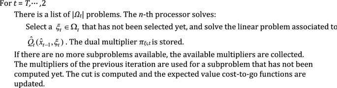
This process is presented graphically in panel (b) of Fig. 5. At stage 3, the blue processor solves the subproblem associated to the first node. When it completes its computation, there are no more subproblems available for that stage, since the red processor has already solved the second node and is now working on the third node. Then the blue processor starts processing the nodes of the second stage. However, in order to compute a cut for stage 2, without having access to the solution information from the subproblem of node 3, the processor uses the subproblem information of node 3 of the cut obtained in the previous iteration. The blue processor is thus able to build a cut, and can start processing the nodes of stage 2.

The following lemma shows that the proposed cuts are valid. The proof can be found in the “Appendix 1”.

Lemma 1

The cuts built in the Async PN scheme are valid cuts.

Following a similar argument as the one presented in Philpott and Guan (2008), we can show that, after a finite number of iterations, no new cuts will be added. The proof can be found in the “Appendix 1”.

Lemma 2

Let ${\mathcal{G}}_{k}^{t,\omega }$ be the set of cuts at stage t, node ω and iteration k. There exists m_t,ω such that $|{\mathcal{G}}_{k}^{t,\omega } | \le m_{t,\omega }$ for all k, 1 ≤ t ≤ T − 1.

It is worth mentioning that as the missing information is not completed using the cuts that are the tightest at the current trial point, as is the case in Philpott and Guan (2008), the convergence might be to a different value. However, as the value function is a lower approximation we can always ensure that the convergence will be an under-estimation. We have also tested the approach of using the cut that maximizes the current trial point, however no considerable difference is observed. In practice, the considered test cases have shown that Async PN presents a convergence behaviour comparable to the one obtained by the other schemes that are implemented in the paper.

As previously said, the authors in Machado et al. (2021) consider a variant in the distribution of the nodes among the processors. Instead of distributing the nodes at each stage, the processors are attached to the nodes of a fixed stage. The authors propose an asynchronous version. The results of the authors vary. On certain instances, such an approach exhibits superior performance relative to a synchronous PS implementation. On other instances, the performance of the proposed method is comparable to a synchronous PS implementation.

4 Case studies

In this section we present results for an inventory control problem and a hydrothermal scheduling problem. The considered case studies aim at present results that correspond to state-of-the-art problem sizes that can be found in the literature. We present problem sizes that correspond to recent SDDP literature in Table 2. Our experimental results can be summarized as follows.

• i Asynchronous computing is not helpful for achieving tight optimality gaps faster. Nevertheless, in certain cases, there is a temporary advantage in the asynchronous PS scheme in early stages of the execution of the algorithm.

• ii The PN scheme performs better than the PS scheme during early stages of the execution of the algorithm.

• iii The PS scheme scales poorly when increasing the number of Monte Carlo samples.

• iv The PN scheme exhibits desirable parallel efficiency properties, nevertheless a competitive implementation is limited to a shared memory setting.

Table 2 Overview of problem sizes in the literature. The problem sizes are ranked according to the year of publication. The dashes indicate that the data was not available in the paper

We proceed by briefly introducing the test cases that we analyze in this work. The models are presented in further detail in the “Appendix 1”.

Inventory control problem We model a stochastic inventory problem with Markovian demand. The objective of the problem is to maximize expected profits by placing optimal order quantities x_tn for products n ∈ N over periods t ∈ H. Demand is satisfied from on-hand inventory v_t−1,n by selling a quantity s_tn of each product. Any excess demand is considered as being lost. We consider a case with 10 products, which is the dimension of the random vector. The problem horizon is equal to 10 stages, with 100 nodes per stage.

Hydrothermal scheduling problem The Brazilian interconnected power system is a multistage stochastic programming problem that has been analyzed extensively in the literature due to its practical relevance (Pereira and Pinto, 1991; Shapiro et al., 2013; Pinto et al., 2013; De Matos et al., 2015; Löhndorf and Shapiro, 2019). The Brazilian power systems comprises, as of 2010, more than 200 power plants. Among these, 141 are hydro units.

The objective of the problem is to determine optimal operation policies for power plants while minimizing operation costs and satisfying demand. Representing the 141 hydro plants as well as their associated inflows results in a high-dimensional dynamic problem. In order to tackle this problem, the literature typically separates it into long-term, medium-term and short-term operational planning. The value functions obtained in long-term operational planning problem are used as input for medium-term planning. The value functions from medium-term planning are then used, in turn, as input for the short-term operational planning problem. The SDDP algorithm is applied in the long-term operational planning problem. The problem is simplified by aggregating reservoirs into equivalent energy reservoirs (Arvanitidits and Rosing, 1970). The literature typically considers 4 energy equivalent reservoirs for this problem instance: North, Northeast, Southeast, South and a Transshipment node. The Transshipment node has no loads or production. The system is presented in Fig. 6.

Fig. 6

Brazilian hydrothermal test case—equivalent reservoirs

The problem aims at satisfying the demand at each node by using the hydro and thermal power of that node, as well as power that is imported from other nodes. However, there is a limit in the power that can flow trough the transmission lines of the electricity network. In the literature, the problem is typically solved for a 60-month planning period. However, in order to represent the continuation of operations at the end of the planning horizon, 60 additional months are considered. This leads to a multi-stage stochastic program in 4 dimensions and 120 stages. We consider a setting with 100 nodes per stage.²

4.1 Experimental results

The computational work is performed on the Lemaitre3 cluster, which is hosted at the Consortium des Equipements de Calcul Intensif (CECI). It comprises 80 compute nodes with two 12-core Intel SkyLake 5118 processors at 2.3 GHz and 95 GB of RAM (3970 MB/core), interconnected with an OmniPath network (OPA-56Gbps). The algorithms are implemented in Julia v0.6 (Bezanson et al., 2017) and JuMP v0.18 (Dunning et al., 2017). The chosen linear programming solver is Gurobi 8.

4.1.1 Synchronous and asynchronous computation

Figure 7 presents the evolution of the optimality gap for all algorithms against run time. The algorithms are run with 20 CPUs. Obtaining a reliable upper bound at each point in time can be very time consuming. Thus, providing a reliable gap evolution can be time consuming as well. Moreover, estimating an upper bound for the Async PS scheme is difficult, as on each CPU there is a policy evolving differently. Therefore, in order to provide a fair comparison between the different schemes, we have pre-calculated a best available lower bound and compared the lower bound evolution of all the algorithms against this best known solution. Concretely, the gap is measured as the relative difference between the lower bound evolution of the algorithm and the “best available lower bound” L that we are able to compute for the problem. What we refer to as the “best available lower bound” L is a lower bound that corresponds to a high-quality policy. The way in which we verify a high-quality policy is by verifying that the relative difference between the upper bound estimate of said policy and L is below 1%. The upper bound estimate for this policy is calculated with a sufficient number of samples so as to ensure a 1% difference between the performance of this policy and L with a confidence of 95%. Once this best lower bound L is calculated, the reported gaps are calculated as follows: (L–L_t) · 100/L, where L_tis the lower bound calculated as each algorithm progresses. More specifically, for the PN schemes and the Sync PS scheme, L_tis the lower bound at the end of iteration t. For the Async PS scheme, each CPU is performing it’s own SDDP run and sharing cuts whenever they are available. Namely, on each CPU the policy is evolving differently. Therefore, L_tcorresponds to the lower bound at the end of iteration t of the fastest CPU.

Fig. 7

Comparison of algorithms. a, b Present the evolution of the optimality gap against time for the inventory test case. c, d Present the evolution of the optimality gap for the hydrothermal problem. a, c Show the gap evolution throughout the entire execution time, with emphasis on presenting the differences when the gap is low. b, d Present a close up at the beginning of the run time, emphasizing the differences between the PS and PN schemes at the early steps of execution

• 1. Parallelizing by Scenario: For the inventory test case, the asynchronous schemes tend to perform better during early iterations, as indicated in panels (a) and (b) of Fig. 7. Instead, for the hydrothermal test case there is not a considerable difference, see panels (c) and (d) of Fig. 7. The difference in the behaviour between both test cases can be explained as follows. As pointed out in De Matos et al. (2015), the expected value cost-to-go function approximations tend to be myopic at early iterations, when the gap is high. This implies that the trial points and the cuts obtained when there is a high gap tend to produce low-quality information. Therefore, the following possibilities can occur:

  • When the algorithm struggles to decrease the gap during early iterations, the synchronous version tends to perform poorly. This is due to the fact that the processors wait for the generation of loose cuts. Instead, an asynchronous version benefits from the fact that the fastest processor is not waiting for these low-quality cuts.

  • On the other hand, when the algorithm manages to reduce the optimality gap during early iterations, the disadvantage of the synchronous version diminishes. This is due to the fact that, since the gap reduces quickly, the value functions are of good quality. Consequently, the synchronous version will wait for useful information.

    The inventory test case corresponds to the former case, whereas the Brazilian hydrothermal test case corresponds to the latter. Panel (a) of Fig. 8 demonstrates that, after 500 scenarios, the gap for the PS methods is above 100% for the inventory test case. Instead, the same number of scenarios analyzed results in a gap below 20% for the hydrothermal test case, as we can observe in panel (c) of Fig. 8. Moreover, as we can observe in panel (b) of Fig. 8, the PS scheme is able to process more scenarios compared to the PN scheme for the inventory test case. Nevertheless, the PS gap is worse, thus supporting the observation that the value functions computed during early steps of the algorithm are poorly approximated.

    Fig. 8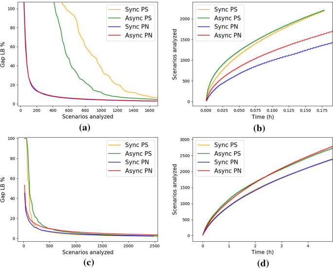

    

    Scenarios analyzed by each method. The scenarios analyzed refers to the number of scenarios visited during the training process for each method. The first row corresponds to the inventory test case, the second row corresponds to the hydrothermal test case. a, c Present the evolution of the optimality gap against the number of scenarios analyzed. b, d Present the number of scenarios analyzed against time

  Despite these observations, we note that there is no significant difference between the synchronous or asynchronous schemes when aiming for tight optimality gaps. This can be observed in Fig. 7. When we target tight gaps, many additional scenarios are required, as we can observe in panels (a) and (c) of Fig. 8. Unfortunately, Async PS is not able to visit many more scenarios than the synchronous counterpart, see panels (b) and (d) of Fig. 8. As a consequence, although Async PS may reduce the optimality gap faster during early iterations, both synchronous and asynchronous schemes achieve similar performance after a significant amount of computation time has elapsed.

• 2. Parallelizing by Node: As seen in panels (b) and (d) of Fig. 8 the asynchronous version is able to process more scenarios as compared to the synchronous counterpart. Nevertheless, the main observation of Fig. 7 is that there is no significant benefit in an asynchronous implementation for parallelizing by node. Both the synchronous and asynchronous parallel node algorithms are attaining comparable performance in terms of gap throughout the entire course of the execution of the algorithms.

In order to evaluate the reproducibility of the results under different runs, 5 repetitions are performed for each method. We report that we observe a similar convergence trend for each repetition. In addition to the experiments shown, an out-of-sample estimation was performed. Every x scenarios used to train the policy, an out-of-sample estimation is done by considering 2000 scenarios not used in the training process. We report the same behaviour already shown in Fig. 7. Concretely, In both test cases the PN schemes tend to perform better at the beginning. For the inventory test case, there is a considerable difference between the Sync PS and Async PS schemes, where the asynchronous version dominates at the beginning.

4.1.2 Parallel node versus parallel scenario

Interestingly, as we can observe in panels (b) and (d) of Fig. 7, the PN strategy is behaving much better than the PS strategy during early iterations. The reason is that, as we discuss previously, the value function approximations tend to be poor in early iterations (De Matos et al., 2015). Thus, at each iteration, the PS version generates several cuts that are loose approximations of the value functions, whereas the PN setting generates a single cut. Nevertheless, if the goal is to obtain tight gaps, the difference is not significant. The reason is that, once value functions of better quality have been obtained by either algorithm, there is a benefit of visiting more than one scenario per iteration. This works in favor of the PS setting.

4.1.3 Scalability of parallel scenario

Panel (a) of Figs. 9, 10 presents the evolution of the PS algorithms when increasing the number of CPUs. Figure 9 corresponds to the inventory test case, and Fig. 10 corresponds to the hydrothermal test case. The target gap for terminating the algorithms is set to 10%. As in the previous experiments, the gap refers to the relative difference between the lower bound and the best available solution. The algorithms present an inherent uncertainty due to the Monte Carlo sampling which is performed in the forward pass. Consequently, the run time itself is random. Therefore, for each CPU count we conduct the experiment 5 times, in order to construct 95% confidence intervals, which are based on Student’s t-distribution. Panels (a) and (b) of Figs. 9 and 10 demonstrate that an initial increase in the number of CPUs results in a notable performance improvement. Nevertheless, there is a point at which this trend is reversed. This is especially true for the inventory test case. We arrive to the same observation when reporting the speedup of the algorithms. Note, in panel (b) of the Figures, that there is a point beyond which the speedup decreases. This is due to the fact that, as more CPUs are introduced, more samples are introduced per iteration. As we have argued, the expected value cost-to-go functions are myopic at early steps. Consequently, more samples tend to introduce information that is not entirely useful for the algorithm, more so in early iterations. This results in a slowdown of the Sync PS algorithm. As the asynchronous version is not waiting for the possibly loose cuts, the effects in the speed up are not as adverse as for the synchronous version. We would also like to point that, as explained by Bertsekas and Tsitsiklis (1989), a synchronous algorithm exhibits a more severe deterioration in scalability when increasing the CPU count, because more problems solved once implies that the slowest one will require more run time. Thus, synchronism affects the algorithm adversely. Note that the problems assignation to the CPUs may affect the performance, showing a closely relation with a job-scheduling problem.

Fig. 9

CPU scalability for the inventory test case

Fig. 10

Hydrothermal test case—CPU scalability

In order to tackle the poor quality of cuts that is produced as a result of the myopic value function that is found at early steps, the cut selection methodology proposed in Löhndorf et al. (2013) is implemented for the Sync PS algorithm. Our choice to focus on the Sync PS algorithm is motivated by the fact that is suffered the most due to the aforementioned effect. This cut selection technique rejects a cut, calculated at point x_t, if the value function is not improved by some > 0 when adding the cut at point x_t. We observe, however, that introducing such a cut selection method has a damping effect: the issue is diminished but is not solved. The cut selection technique helps by not adding some non-useful cuts to the linear programs, nevertheless the computational resources are wasted as several scenarios end up building non-useful cuts. Concretely, resources are wasted by solving linear programs that end up building non-useful cuts.

4.1.4 Parallel node scalability

Panel (a) of Figs. 9, 10 presents the performance when increasing the number of CPUs for the parallel node setting. As in the previous paragraph, the target optimality gap is set to 10% and 95% confidence intervals are presented. Note that the performance of the algorithm improves with additional CPUs. Since the algorithm is building one cut per iteration, as more CPUs are introduced, that single cut is computed faster. This is an important difference as compared to the PS scheme, where the speedup can decrease.

Although this scheme exhibits favorable scalability behavior, it is limited to a shared memory setting. As stated in Sect. 3.1.2 the reason behind this limitation is that the solve time of a subproblem is comparable to the startup cost of a worker in a distributed memory setting. Concretely, after some hundred of iterations the solve time per subproblem for both test cases ranges in a few milliseconds, a time which is comparable to the startup cost which is about 3 ms. Therefore, the latency of the network becomes an issue.

5 Conclusions

In this paper we propose a family of parallel schemes for SDDP. These schemes are differentiated along two dimensions: (i) using parallel processors in order to distribute computation per Monte Carlo sample of the forward pass (per scenario) or per node of the lattice at every stage of the problem (per node); (ii) implementing the exchange of information among processors in a synchronous or asynchronous fashion. We compare the performance of these algorithms in two case studies: (i) an inventory management problem, and (ii) an instance of the Brazilian hydrothermal scheduling problem. The case studies deliver consistent messages, which we summarize below in the form of four conclusions.

(i) Asynchronous computing is not helpful in the studied experiments, when the goal is to achieve a tight optimality gap in a shorter time. Asynchronous schemes, on the other hand, may be beneficial at early stages of the Parallel Scenario strategy. (ii) We have proposed a Parallel Node strategy for SDDP, which performs better at early iterations than the traditional parallel scheme for SDDP. (iii) Parallel schemes that are based on increasing the number of scenarios which are processed during the forward pass, may not scale well with extra CPUs. This is the case for the PS scheme. (iv) The Parallel Node strategy presents desirable CPU scalability properties, but only in a shared memory setting.

We would also like to highlight that synchronous schemes are easier to fully reproduce. While reproducing results may be easier, it still remains difficult. Full reproducibility of a synchronous parallel scheme entails solving node problems and updating cuts in a fixed order. This naturally decreases the benefits of parallel computing, since an idle processor would need to wait for its turn according to the fixed sequence. The reproducibility of asynchronous schemes is considerably more involved, as it would require to pre-define the exact sequence of events and the exact exchange of information between CPUs. This introduces synchronization between CPUs and undermines the purpose of an asynchronous implementation. The implementation and study of full reproducibility is beyond the scope of the present paper.

In our work we have indicated some of the weaknesses in the parallelization of SDDP. On the one hand, we have empirically demonstrated scalability issues with the commonly proposed parallel scheme. On the other hand, we have proposed a new set of parallel schemes, with better scalability properties. However, our proposed algorithms which present better scalability with respect to CPU count are restricted to a shared memory setting. This observation motivates future research into scalable parallel SDDP schemes based on backward dynamic programming. These schemes, which present desirable scalability properties, are closer to the per-node strategy, but are also implementable in distributed memory settings, such as high performance computing clusters.

Appendices

Appendix: Inventory control problem

The inventory control problem can be modeled as a multistage stochastic problem. The uncertainty in the problem is due to stochastic demand, which is assumed to follow a Markov Chain. The cost-to-go function $Q_{t} (v_{t - 1} ,\xi_{t} )$ is computed by solving the following problem:

$$ \begin{aligned} & \max \;\sum\limits_{{n \in {\mathcal{N}}}} P \cdot s_{t,n} - HC \cdot v_{t,n} - PC \cdot x_{t,n} + {\mathcal{Q}}_{t + 1} (v_{t} ,\xi_{t} ) \\ & \;\;\;\;\;\;\;\;\;\;\;\;\;\;\;\;\;\;\;\;\;\;\;\;\;s.t.\;v_{t,n} = v_{t - 1,n} + x_{t,n} - s_{t,n} \quad n \in {\mathcal{N}} \\ & \;\;\;\;\;\;\;\;\;\;\;\;\;\;\;\;\;\;\;\;\;\;\;\;\;s_{t,n} \le v_{t - 1,n} \quad \quad \quad n \in {\mathcal{N}} \\ & \;\;\;\;\;\;\;\;\;\;\;\;\;\;\;\;\;\;\;\;\;\;\;\;\;s_{t,n} \le D_{t,n} (\xi_{t} ) \, \quad n \in {\mathcal{N}} \\ & \;\;\;\;\;\;\;\;\;\;\;\;\;\;\;\;\;\;\;\;\;\;\;\;\;v_{t,n} \le C \, \quad \quad \quad \, \quad n \in {\mathcal{N}} \\ & \;\;\;\;\;\;\;\;\;\;\;\;\;\;\;\;\;\;\;\;\;\;\;\;\;\;v_{t,n} ,s_{t,n} ,x_{t,n} \ge 0\quad \quad \quad n \in {\mathcal{N}} \\ \end{aligned} $$

The variables are given as follows:

• v_t,n: The state variable, which represents the on-hand inventory for product n ∈ N.

• s_t,n: Variable representing the amount of sold items for product n ∈ N.

• x_t,n : Variable representing the ordered quantities for product n ∈ N.

The parameters can be described as follows:

• P: The sales price.

• HC: The inventory holding cost.

• PC: the purchase cost.

• D_t,n: The demand for product n ∈ N.

• C: The inventory capacity.

The problem is set up for 10 products. This is the dimension of the random vector. The time horizon is equal to 10 stages. We consider 100 nodes per stage.

Hydrothermal Scheduling problem

We use a transportation model to approximate the operation of the transmission network. The cost to go function $Q_{t} (v_{t - 1} ,\xi_{t} )$ can then be computed by solving the following problem:

$$ \begin{aligned} & \min \;\sum\limits_{{i \in {\mathcal{G}}}} {M_{i} } \cdot g_{t,i} + {\text{VOLL}}\sum\limits_{{n \in {\mathcal{N}}}} l s_{t,n} + {\mathcal{Q}}_{t + 1} (v_{t} ,\xi_{t} ) \\ & \quad \quad \quad \quad \quad \quad s.t.\;v_{t,n} = v_{t - 1,n} + A_{t,n} (\xi_{t} ) - q_{t,n} - s_{t,n} \, \quad n \quad \in {\mathcal{N}} \\ & \quad \quad \quad \quad \quad \quad \quad q_{t,n} + \sum\limits_{{i \in {\mathcal{G}}}} {g_{t,i} } + \sum\limits_{{i \in {\mathcal{F}}_{n} }} {f_{t,i} } = L_{t,n} \, \quad n \in {\mathcal{N}} \\ & \quad \quad \quad \quad \quad \quad \quad g_{t} \le \overline{G} \\ & \quad \quad \quad \quad \quad \quad \quad v_{t} \le \overline{V} \\ & \quad \quad \quad \quad \quad \quad \quad q_{t} \le \overline{Q} \\ & \quad \quad \quad \quad \quad \quad \quad f_{t} \le \overline{F} \\ & \quad \quad \quad \quad \quad \quad \quad g_{t} ,ls_{t} ,v_{t} ,q_{t} ,s_{t} ,f_{t} \ge 0 \\ \end{aligned} $$

The variables can be described as follows:

• v_t: The state variable vector, which represents the stored energy of the equivalent reservoir.

• q_t,s_t : Decision variables which represent the generated hydro energy and the spillage, respectively.

• ls_tn : Decision variable which represents load shedding.

• g_t: The vector of generated power from thermal plant i ∈ G.

The parameters can be described as follows:

• M_i: The generation cost of thermal plan i ∈ G.

• V OLL: The value of lost load.

• P_i: The hydro generation coefficient of hydro plant i ∈ H.

• A_t: The inflow vector.

• L_t: Load at stage t.

• G,¯ V ,¯ Q,¯ F¯ : Physical upper limits on the variables.

Further details for the Brazilian hydrothermal model, and the description of the data, can be found in Shapiro et al. (2013).

Convergence of the async PN scheme

The proposed strategy to build cuts for the Async PN scheme is a valid strategy, as the following lemma shows.

Lemma 1

The cuts built in the Async PN scheme are valid cuts.

Proof

Let $\hat{x}_{t - 1}^{k}$ be the obtained trial point for stage t − 1 at iteration k. Consider the cut for the cost-to-go function.

$Q_{t} (x_{t - 1} ,\xi_{t} )$, which is given by

$$ Q_{t} (x_{t - 1} ,\xi_{t} ) \ge \alpha_{{\xi_{t} ,t}}^{k} + \beta_{{\xi_{t} ,t}}^{k} \cdot x_{t - 1} $$

(1)

The expected cost-to-go function satisfies

$$ {\mathcal{Q}}_{t} (x_{t - 1} ,\xi_{t - 1} ) = \sum\limits_{{\xi_{t} \in \Omega_{t} }} {Q_{t} } (x_{t - 1} ,\xi_{t} ) \cdot P(\xi_{t} |\xi_{t - 1} ) $$

(2)

Then, a cut for ${\mathcal{Q}}_{t} (x_{t - 1} ,\xi_{t - 1} )$ is given by

$$ {\mathcal{Q}}_{t} (x_{t - 1} ,\xi_{t - 1} ) \ge \sum\limits_{{\xi_{t} \in \Omega_{t} }} {\alpha_{{\xi_{t} ,t}}^{k} } \cdot P(\xi_{t} |\xi_{t - 1} ) + \sum\limits_{{\xi_{t} \in \Omega_{t} }} {\beta_{{\xi_{t} ,t}}^{k} } \cdot P(\xi_{t} |\xi_{t - 1} ) \cdot x_{t - 1} $$

(3)

Let us now build a cut for the expected cost-to-go function at iteration k + 1 using incomplete information. Assume that, at iteration k + 1, we do not have access to the solution information of outcome $\hat{\xi }_{t}$. Note that, as Eq. (1) holds for any x_t−1, and given Eq. (2), we can write

$$ \begin{aligned} & {\mathcal{Q}}_{t} (x_{t - 1} ,\xi_{t - 1} ) \ge \sum\limits_{{\xi_{t} \in \Omega_{t} - \{ \hat{\xi }_{t} \} }} {\alpha_{{\xi_{t} ,t}}^{k + 1} } \cdot P(\xi_{t} |\xi_{t - 1} ) + \alpha_{{\hat{\xi }_{t} ,t}}^{k} \cdot P(\hat{\xi }_{t} |\xi_{t - 1} ) \\ & \quad + [\sum\limits_{{\xi_{t} \in \Omega_{t} - \{ \hat{\xi }_{t} \} }} {\beta_{{\xi_{t} ,t}}^{k + 1} } \cdot P(\xi_{t} |\xi_{t - 1} ) + \beta_{{\hat{\xi }_{t} ,t}}^{k} \cdot P(\hat{\xi }_{t} |\xi_{t - 1} )] \cdot x_{t - 1} \\ \end{aligned} $$

(4)

Note that, in Eq. 4, the missing information, at iteration k + 1, of outcome $\hat{\xi }_{t}$ is completed by using the information of the previous iteration, namely by using the cut coefficients $\alpha_{{\hat{\xi }_{t} ,t}}^{k} ,\beta_{{\hat{\xi }_{t} ,t}}^{k}$ of the previous iteration.

In Philpott and Guan (2008) the authors show that any sequence of cuts will necessarily be finite, in the sense that after a finite number of iterations no new cuts will be computed. Concretely, the following lemma, which is just an adaptation of the proof shown in Philpott and Guan (2008), proves that after a finite number of iterations the algorithm will not produce new cuts.

Lemma 2

Let ${\mathcal{G}}_{k}^{t,\omega }$ be the set of cuts at stage t, node ω and iteration k. There exists m_t,ω such that $|{\mathcal{G}}_{k}^{t,\omega } | \le m_{t,\omega }$ for all k, 1 ≤ t ≤ T − 1.

Proof

Let’s proceed by induction on t. For t = T − 1. Note that as there are no cuts in the last stage, the set of multipliers in the last stage is given by,

$$ \{ \pi |\pi^{T} \cdot A_{T} (\omega ) \le c_{T}^{T} (\omega )\} $$

Thus, there are at most let’s say M_T,ω possibilities for multipliers. Assuming there are N_t nodes for stage t, then it implies that at stage T there are at most $\prod\nolimits_{i = 1}^{{N_{T} }} {M_{{T,\omega_{i} }} }$ combinations of multipliers. As a consequence for any node ω at stage T − 1 there are at most $m_{T - 1,\omega } : = \prod\nolimits_{i = 1}^{{N_{T} }} {M_{{T,\omega_{i} }} }$ possibilities to build a cut. Let’s now assume that for t we have m_t,ω such that $|{\mathcal{G}}_{k}^{t,\omega } | \le m_{t,\omega }$ for all k. We have to show the property holds for t − 1.

Due to the assumption, we know that for node ω in stage t, $|{\mathcal{G}}_{k}^{t,\omega } | \le m_{t,\omega }$, in particular this implies that there exists a $\widehat{k}$ such that ${\mathcal{G}}_{{\hat{k}}}^{t,\omega } = {\mathcal{G}}_{k}^{t,\omega }$ for all k > $\widehat{k}$, and so any cut after iteration $\widehat{k}$ is already in the set of cuts. Then after iteration$\widehat{k}$, the linear program of node ω at stage t won’t have new cuts. As a consequence the set of multipliers for node ω at stage t is finite, say M_t,ω. This implies that at stage t there are $\prod\nolimits_{i = 1}^{{N_{t} }} {M_{{t,\omega_{i} }} }$ possible combinations of multipliers. Therefore, for any node ω at stage t − 1 there will be at most $m_{t - 1,\omega } : = \prod\nolimits_{i = 1}^{{N_{t} }} {M_{{t,\omega_{i} }} }$ possibilities to build a cut, which proves the result.

References

Aravena I, Papavasiliou A (2020) Asynchronous lagrangian scenario decomposition. Mathematical Programming Computation pp 1–50
Arvanitidits NV, Rosing J (1970) Composite representation of a multireservoir hydroelectric power system. IEEE Trans Power Appar Syst 2:319–326
Asamov T, Powell WB (2018) Regularized decomposition of high-dimensional multistage stochastic programs with markov uncertainty. SIAM J Optim 28(1):575–595
Bertsekas DP, Tsitsiklis JN (1989) Parallel and distributed computation: numerical methods, vol 23. Prentice hall Englewood Cliffs, NJ
Bezanson J, Edelman A, Karpinski S, Shah VB (2017) Julia: A fresh approach to numerical computing.
Birge JR, Louveaux F (2011) Introduction to stochastic programming. Springer Science & Business Media
da Silva EL, Finardi EC (2003) Parallel processing applied to the planning of hydrothermal systems. IEEE Trans Parallel Distrib Syst 14(8):721–729
De Matos V, Philpott AB, Finardi EC, Guan Z (2010) Solving long-term hydro-thermal scheduling problems. Technical report, Electric Power Optimization Centre, University of Auckland, Tech. rep.
De Matos VL, Philpott AB, Finardi EC (2015) Improving the performance of stochastic dual dynamic programming. J Comput Appl Math 290:196–208
Dowson O, Kapelevich L (2021) Sddp. jl: a julia package for stochastic dual dynamic programming. INFORMS Journal on Computing 33(1):27–33
Dowson O, Philpott A, Mason A, Downward A (2019) A multi-stage stochastic optimization model of a pastoral dairy farm. Eur J Oper Res 274(3):1077–1089
Dunning I, Huchette J, Lubin M (2017) Jump: A modeling language for mathematical optimization. SIAM Rev 59(2):295–320. https://doi.org/10.1137/15M1020575
Flach B, Barroso L, Pereira M (2010) Long-term optimal allocation of hydro generation for a price-maker company in a competitive market: latest developments and a stochastic dual dynamic programming approach. IET Gener Transm Distrib 4(2):299–314
Guigues V (2017) Dual dynamic programing with cut selection: Convergence proof and numerical experiments. Eur J Oper Res 258(1):47–57
Guigues V, Bandarra M (2019) Single cut and multicut sddp with cut selection for multistage stochastic linear programs: convergence proof and numerical experiments. arXiv preprint arXiv:190206757
Helseth A, Braaten H (2015) Efficient parallelization of the stochastic dual dynamic programming algorithm applied to hydropower scheduling. Energies 8(12):14287–14297
Kaneda T, Scieur D, Cambier L, Henneaux P (2018) Optimal management of storage for offsetting solar power uncertainty using multistage stochastic programming. In: 2018 Power Systems Computation Conference (PSCC), IEEE, pp 1–7
Löhndorf N, Shapiro A (2019) Modeling time-dependent randomness in stochastic dual dynamic programming. Eur J Oper Res 273(2):650–661
Löhndorf N, Wozabal D (2020) Gas storage valuation in incomplete markets. European Journal of Operational Research
Löhndorf N, Wozabal D, Minner S (2013) Optimizing trading decisions for hydro storage systems using approximate dual dynamic programming. Oper Res 61(4):810–823
Machado FD, Diniz AL, Borges CL, Brandão LC (2021) Asynchronous parallel stochastic dual dynamic programming applied to hydrothermal generation planning. Electric Power Systems Research 191:106907
Papavasiliou A, Oren SS, Rountree B (2014) Applying high performance computing to transmissionconstrained stochastic unit commitment for renewable energy integration. IEEE Trans Power Syst 30(3):1109–1120
Papavasiliou A, Mou Y, Cambier L, Scieur D (2017) Application of stochastic dual dynamic programming to the real-time dispatch of storage under renewable supply uncertainty. IEEE Transactions on Sustainable Energy 9(2):547–558
Pereira MV, Pinto LM (1991) Multi-stage stochastic optimization applied to energy planning. Math Program 52(1–3):359–375
Philpott AB, De Matos VL (2012) Dynamic sampling algorithms for multi-stage stochastic programs with risk aversion. Eur J Oper Res 218(2):470–483
Philpott AB, Guan Z (2008) On the convergence of stochastic dual dynamic programming and related methods. Oper Res Lett 36(4):450–455
Philpott AB, de Matos VL, Kapelevich L (2018) Distributionally robust sddp. CMS 15(3–4):431–454
Pinto RJ, Borges CT, Maceira ME (2013) An efficient parallel algorithm for large scale hydrothermal system operation planning. IEEE Trans Power Syst 28(4):4888–4896
Shapiro A (2011) Analysis of stochastic dual dynamic programming method. Eur J Oper Res 209(1):63–72
Shapiro A, Tekaya W, da Costa JP, Soares MP (2013) Risk neutral and risk averse stochastic dual dynamic programming method. Eur J Oper Res 224(2):375–391
Van Ackooij W, de Oliveira W, Song Y (2019) On level regularization with normal solutions in decomposition methods for multistage stochastic programming problems. Comput Optim Appl 74(1):1–42
Acknowledgements
Computational resources have been provided by the Consortium des Equipements de Calcul Intensif (CECI), funded by the Fonds de la Recherche Scientifique de Belgique (F.R.S.-FNRS) under Grant No. 2.5020.11 and by the Walloon Region. The first and second author have been supported financially by the Bauchau family in the context of the Bauchau prize which is administered by UCLouvain. This work was supported in part by the European Commission’s Horizon 2020 Framework Program under grant agreement No 864537 (FEVER Project).
Funding
Université Catholique de Louvain.
Author information
Authors and Affiliations
Corresponding author
Additional information
Publisher's Note
Springer Nature remains neutral with regard to jurisdictional claims in published maps and institutional affiliations.
The original version of this article was revised due to a retrospective Open Access order.