
Abstract
Universities and research institutions have the responsibility to produce science and to provide training to new generations of researchers. In this paper, we propose a model to analyze the determinants of a senior scientist’s decisions about allocating time between these tasks. The results of this decision depend upon the characteristics of the research project, the senior scientist’s concern for training and the expected innate ability of the junior scientist involved. We analyze the role that a regulator can play in defining both the value of scientific projects and the future population of independent scientists.


Notes
1 In the US, the Bay-Dole Act puts incentices on research and transfer and commercialization of university innovations. In the UK, the Research Assesment Exercise (RAE) has an importnat impact on funding. Many countries university founding depends to certain extent on research results (publications, patents, licenses)
2 For example, the ”Patterns and Trends Report 2011 in UK Higher Education” reports that in the UK over the last 10 years (since 2000/01) the (full-time) postgraduate numbers have increased by 73.1 per cent (compared with an increase of 28.5 per cent for full-time undergraduates over the same period).
3 Obviously, an alternative to training one’s own researchers is to attract researchers trained elsewere. While this is an interesting idea, we choose to ignore this topic in this paper.
4 It seems that there can be a mismatch in the perceptions of the supervisor and of doctoral students with respect to accessibility. In a study on the provisions of PhD training in biomedical research PhD programs, virtually all supervisors reported meeting frequently with their students, whereas 1/4 of the students reported problems in accessing their supervisor (Frame and Allen 2002).
5Nerad and Cerny (1999) also survey the perspective on postdoctoral employment in the U.S. and report that there exists a generalized discontent on behalf of postdoctoral researchers. The length of postdoctoral appointments has increased and these appointments are increasingly being seen as ‘holding base’, rather than being an important step in a young researcher’s career.
6 This does not mean that the junior scientist’s innate ability is public information. It is ex-ante unknown by both participants. Even though a student is selected to participate in a graduate programme or in a lab according to a GRE score, and other internal admission criteria of a department, significant uncertainty remains in predicting if a student has the potential to become a successful independent researcher (Lovitts 2005).
7 In our model, we could also discuss the researcher preferences, but this is not the main aspect of the analysis.
8 In Section 4, we endogenize the decision of the senior scientist concerning the time she works. For now, we assume that t is exogenously given.
9 In our model, there is always symmetric information about the junior scientist’s innate ability. Under complete information senior and junior know that his innate ability is \(\hat {a};\) under ignorance they expect it to be \(E(\tilde {a})\).
10 For the senior scientist, training may increase visibility and reputation when the young professional is a productive member. The model also includes the trainer’s inner satisfaction in passing along knowledge.
11 One can also argue that the senior researcher has incentives to devote a minimum amount of time to research so as to produce a valuable knowledge. Valuable projects in the past may improve the possibility of financing for future scientific projects. However, for completeness, the case β>δ t is included in the working paper version of the model: Freitas and Macho-Stadler (2011).
12 Given our assumption β≤δ t we do not have the other extreme case: when the senior scientist’s concern about the junior’s training is high as compared to the time available that she decides only to perform training. This posibility is taken into consideration in a previous version of our model (Freitas-and-Macho-Stadler:2012) where β is not constrained from above.
13 The function v ∗(a) is convex in a and q ∗(a) is linear in a.
14 With perfect information about the junior scientist’s innate ability \(\hat {a} =E(\tilde {a})\), and the ex-post and ex-ante values of the project (resp., the junior capability) are identical.
15 \(x=e_{R}^{\ast }(E(\tilde {a}))\) and \(y=e_{G}^{\ast }(E(\tilde {a}))\) are the optimal decisions of the senior to perform research and training, respectively, based on the expected capability of the junior.
16 Note that this comparison is between the decision of the senior scientist with full information and the decision under ignorance, but none of these decisions may be in accordance with the social optimum. The distortion at the bottom that leads senior scientists to train more juniors under ignorance may be good from a social point of view. The distortion at the top may be a serious concern for the society and may push to be interested in guaranteeing that excellent projects and high-potential junior scientists are better identified. We discuss these issues in Section 5.
Fig. 1 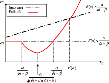
Comparison of the ex-post value of the project under full information \(v^{\ast }(\hat {a})\) and ignorace \( v^{o}(\hat {a},E(a))\)
17 More precisely, for \(E(\tilde {a})\leq \left (\frac {\hat {a}\alpha }{2(\alpha + \hat {a}\beta )}\right )^{\frac {1}{2}}\).
18 If the cost c is smaller that a δ/2 the optimal time goes to infinite. In this case it would be natural to include a maximum time limit T. We will comment on this assumption later, but we will concentrate on the case where c is high for the sake of simplicity.
19 For completeness, let us remark that if c is not constrained from below (i.e., there is a maximum amount of time T that the senior scientist has available), the results will be similar, except for low costs c \(\left (c\leq \frac {a\delta }{2}\right ) \) and/or T small enough \(\left (T<\frac { \left \vert \alpha -a\beta \right \vert }{a\delta }\right ) \). In these cases, the senior chooses to work for all the available time and she allocates all the time T either to research (α>a β) or to training (α<a β) (except if α=a β, case where she is indifferent). Changes in α or in β do not affect the total time allocated to work and only discrete changes may affect to which task this time T is allocated. In these cases, only changes of the time available for these activities may have an effect on the senior scientist’s behavior.
20 In some cases the regulator can also change the time available for these tasks t (for example, by reducing the senior’s involvement in other time-consuming tasks, such as administrative ones).

References
Banal-Estañol A, Macho-Stadler I (2010) Scientific and commercial incentives in R and D: research vs. development. J Econ Manag Strateg 19 (1): 185–221
Cech T, Bond E (2004) Managing your own labScience. Sci 304(5678):1717
Frame I, Allen L (2002) A flexible approach to phd research training. Qual Assur Educ 12 (2): 98–103
Freitas A, Macho-Stadler I (2011) On the joint production of research and training, working paper 531, Barcelona GSE
Golde C (2000) Should I stay or should I go? Student descriptions of the doctoral attrition process. Rev High Educ 23 (2): 199–227
Lacetera N, Zirulia L (2008) Knowledge spillovers, competition, and taste for science in a model of R&D incentive provision. Universita’ di Bologna, Working Paper
Lovitts B E (2001) Leaving the ivory tower: the causes and consequences of departure from doctoral study. Rowman & Littlefield, Lanham, MA
Lovitts B E (2005) Being a good course-taker is not enough: a theoretical perspective on the transition to independent research. Stud High Educ 30 (2): 137–154
Nerad M, Cerny J (1999) Postdoctoral patterns, career advancement, and problems. Sci 285 (5433): 1533–1535
Paglis L, Green S, Bauer T (2006) Does advisor mentoring add value? A longitudinal study of mentoring and doctoral student outcomes. Res High Educ 47 (5): 451–476
Pole C, Sprokkereef A, Burgess, Robert G, Lakin E (1997) Supervision of doctoral students in the natural sciences: expectations and experiences. Assess Eval High Educ 22 (1): 49–63
Puljak L (2006) Career blocker: bad advisors, in http://sciencecareers.sciencemag.org.
Stephan P E, Levin S G (1992) Striking the mother lode in science: the importance of age, place and time. Oxford University Press, New York
Vogel G (1999) A day in the life of a topflight lab. Sci 285: 1531–1532
Walckiers A (2008) Multidimensional contracts with task-specific productivities: an application to universities. Int Tax Public Financ 15: 165–198
Author information
Authors and Affiliations
Corresponding author
Additional information
We thank David Pérez Castrillo and a referee for their comments. We gratefully acknowledge the financial support from the research grants (ECO2009-07616 and ECO2012-31962) and Generalitat de Catalunya (2009SGR-169). The second author is fellow of MOVE.
Appendix :
Appendix :
1.1 Proof of Lemma 1
The program can be rewritten as
The Lagrangian of this program is \(\mathcal {L}=\alpha e_{R}+a\delta \left (t-e_{R}\right ) e_{R}+\beta a\left (t-e_{R}\right ) +\lambda e_{R}+\mu \left (t-e_{R}\right ) \), which FOC is:
Then cases to consider are (1) λ=0, μ=0 and \(e_{R}=\frac {a\delta t+\alpha -\beta a}{ 2a\delta }\), which is a candidate when \(\frac {a\delta t+\alpha -\beta a}{ 2a\delta }\geq 0\) and \(\frac {a\delta t+\alpha -\beta a}{2a\delta }\leq t\), or equivalent, when \(\alpha +a\left (\delta t-\beta \right ) \geq 0\) (which is always the case since δ t≥β≥0) and \(\alpha -a\left (\delta t+\beta \right ) \leq 0\). (2) λ>0, μ=0 and e R =0, which is a candidate when \(\alpha +a\left (\delta t-\beta \right ) \leq 0\) and \(\alpha -a\left (\delta t+\beta \right ) \leq 0\). This case never occurs since δ t≥β≥0. (3) λ=0, μ>0 and e R =t, which asks for \(\alpha -a\left (\delta t+\beta \right ) \geq 0\). Finally, the combination of these cases gives the results presented in the Lemma.
1.2 Proof of Lemma 3
We proceed for simplicity by regions of parameters:
Case 1: α−a β>0
In this case:
Step (i) Let’s first consider the function u(t)=α t. The maximization problem is
The Lagrangian function is \(\mathcal {L}=\alpha t-\frac {c}{2}t^{2}+\lambda (\frac {\alpha -a\beta }{a\delta }-t)+\mu t\). The FOC is
Then the possibilities are (i.1) λ=0 and μ=0, then \(t=\frac { \alpha }{c}\), which is a candidate when \(\frac {\alpha }{c}\leq \frac {\alpha -a\beta }{a\delta }\Longleftrightarrow \frac {a\delta \alpha }{\alpha -a\beta }\leq c\). (ii.2) λ>0 and μ=0, then \(t=\frac {\alpha -a\beta }{ a\delta }\), which is a candidate when \(\alpha -c(\frac {\alpha -a\beta }{ a\delta })>0\), i.e., \(\frac {\alpha }{c}>\frac {\alpha -a\beta }{a\delta } \Longleftrightarrow \frac {a\delta \alpha }{\alpha -a\beta }>c\). (ii.3) λ=0 and μ>0, then t=0, which is a candidate if α<0 which is never the case. Step (ii) Let’s now consider the function \(u(t)=\frac {\left (\alpha +at\delta \right )^{2}-(a\beta )^{2}}{4a\delta }+\frac {2a\beta (a\delta t-\alpha +a\beta )}{4a\delta }\). The maximization problem is
The Lagrangian is \(\mathcal {L}=\frac {\left (\alpha +at\delta \right ) ^{2}-(a\beta )^{2}}{4a\delta }+\frac {2a\beta (a\delta t-\alpha +a\beta )}{ 4a\delta }-\frac {c}{2}t^{2}+\lambda (t-\frac {\alpha -a\beta }{a\delta })\). The FOC is
Then, the possibilities are: (ii.1) λ=0 and \(t=\frac {\alpha +a\beta }{2c-a\delta }\), which is a candidate when \(\frac {\alpha +a\beta }{ 2c-a\delta }>\frac {\alpha -a\beta }{a\delta }\) or, equivalently, when \(\frac { a\delta \alpha }{\alpha -a\beta }\geq c\). (ii.2) λ>0 and \(t=\frac { \alpha -a\beta }{a\delta }\), which asks for \(\frac{a\delta \alpha }{\alpha -a\beta }<c. \), or equivalently \(\frac {a\delta \alpha }{\alpha -a\beta }<c\). Step (iii) Comparing the results from the previews steps, and realizing that the candidate for solution in one of cases is a possible solution in the other case we obtain the result presented in the Lemma.
Case 2: α−a β<0
Here we have:
Step (i) Let’s consider the function u(t)=a β t. The maximization problem is
The Lagrangian function is \(\mathcal {L}=a\beta t-\frac {c}{2}t^{2}+\lambda (\frac {a\beta -\alpha }{a\delta }-t)+\mu t\). The FOC is
Then the possibilities are (i.1) λ=0 and μ=0 which gives \(t= \frac {a\beta }{c}\), which is a candidate when \(\frac {a\beta }{c}\leq \frac { a\beta -\alpha }{a\delta }\Longleftrightarrow \frac {\beta a^{2}\delta }{ a\beta -\alpha }\leq c\). (ii.2) λ>0 and μ=0, and \(t=\frac { a\beta -\alpha }{a\delta }\), which is a candidate when \(\alpha -c\left (\frac {a\beta -\alpha }{a\delta }\right ) >0\), i.e., \(\frac {\alpha }{c}>\frac { a\beta -\alpha }{a\delta }\Longleftrightarrow \frac {\beta a^{2}\delta }{ a\beta -\alpha }>c\). (ii.2) λ=0 and μ>0, and t=0, which is a candidate when a β<0, which is never the case. Step (ii) Let’s now consider the function \(u(t)=\frac {\left (\alpha +at\delta \right )^{2}-(a\beta )^{2}}{4a\delta }+\frac {2a\beta (a\delta t-\alpha +a\beta )}{4a\delta }\). The maximization problem is
The Lagrangian function is \(\mathcal {L}=\frac {\left (\alpha +at\delta \right )^{2}-(a\beta )^{2}}{4a\delta }+\frac {2a\beta (a\delta t-\alpha +a\beta )}{4a\delta }-\frac {c}{2}t^{2}+\lambda (t-\frac {a\beta -\alpha }{ a\delta })\). The FOC is
Then, the possibilities are: (ii.1) λ=0 and \(t=\frac {\alpha +a\beta }{2c-a\delta }\), which is a candidate when \(\frac {\alpha +a\beta }{ 2c-a\delta }>\frac {a\beta -\alpha }{a\delta }\) or, equivalently, when \(\frac { \beta a^{2}\delta }{a\beta -\alpha }>c\). Note that \(\frac {\beta a^{2}\delta }{a\beta -\alpha }<\frac {a\delta }{2}\) (ii.2) λ>0 and \(t=\frac { a\beta -\alpha }{a\delta }\), which asks for \(\frac {\alpha +a\delta (-\frac { \alpha -a\beta }{a\delta })+a\beta }{2}-c(\frac {a\beta -\alpha }{a\delta } )<0\), or equivalently \(\frac {\beta a^{2}\delta }{a\beta -\alpha }<c\). Step (iii). Comparing the results from the previews steps, and realizing that the candidate for solution in one of cases is a possible solution in the other case we obtain the result presented in the Lemma.
Case 3: α−a β=0
In this case:
Then the maximization problem of the senior is:
The Lagrangian function is \(\mathcal {L}=\frac {2t\left (\alpha +\beta a\right ) +a\delta t^{2}}{4}-\frac {c}{2}t^{2}+\lambda t\). The FOC is
Then, the possibilities are: (i) λ=0 and \(t=\frac {\alpha +a\beta }{2c-a\delta }\), which is a candidate when \(\frac {\alpha +a\beta }{ 2c-a\delta }\geq 0\) or, equivalently, when \(c>\frac {a\delta }{2}\). (ii) λ>0 and t=0, which asks for \(\frac {\alpha +a\beta }{2}<0\), which is never the case.
1.3 Proof of Lemma 5
For the case β=0 and δ=1, we consider the candidates that satisfy a 2−(g T+A)a+α g≥0 and a 2−(g T+A)a+α g<0 sequentially and then we provide the solution as function of the parameters.
Step 1: a 2−(g T+A)a+α g≥0
The utility function to be considered is \(u^{\ast }(t)=\alpha \left (T-\frac { a-A}{g}\right ) \).
Depending on the parameters, the values of a such that a 2−(g T+A)a+α g=0 (they only exist if (g T+A)2−4α g≥0) will lie, or not, in the interval where the junior’s ability is defined, \( \left [ A,gT+A\right ] \). When a=A, a 2−(g T+A)a+α g has a positive value if A T≤α, and a negative value otherwise. When a=g T+A, the value for a 2−(g T+A)a+α g is always positive. Hence we can define 3 possible regions to attain a solution: a) when A T≤α and (g T+A)2−4α g≥0; b) when A T≤α and (g T+A)2−4α g<0; and c) when A T>α and (g T+A)2−4α g≥0. The One last case could be A T>α and (g T+A)2−4α g<0, however it is not possible since this would mean that the function never has negative values and, simultaneously, has a negative value when a=A.
Case a) A T≤α and (g T+A)2−4α g≥0
In this case the optimal ability lies in either one of the two following regions: \(A\leq a\leq \frac {gT+A-\sqrt {(gT+A)^{2}-4\alpha g}}{2}\) or \(\frac { gT+A+\sqrt [2]{(gT+A)^{2}-4\alpha g}}{2}\leq a\leq gT+A\). We first formalize the problem with respect to the first region:
The lagrangian is \(\mathcal {L}=\alpha \left (T-\frac {a-A}{g}\right ) +\lambda (a-A)+\mu (\frac {gT+A-\sqrt {(gT+A)^{2}-4\alpha g}}{2}-a)\). The FOC is \(- \frac {\alpha }{g}+\lambda -\mu =0\)
There are two possible cases for the lagrangian multipliers:
1) λ>0, μ=0. a=A is a candidate.
2) λ>0, μ>0. This holds when \(A=\frac {gT+A-\sqrt { (gT+A)^{2}-4\alpha g}}{2}\Leftrightarrow AT=\alpha \) which is a particular case of 1). Hence a=A is again a candidate.
Formalizing the problem with respect to the second region, the FOC is:
One possible case exists for the lagrange multiplier:
1) λ=0, μ>0. In this case, \(a=\frac {gT+A+\sqrt { (gT+A)^{2}-4\alpha g}}{2}\) is a candidate.
Since the utility function is decreasing in a, a=A is a candidate for the optimal ability.
Case b) A T≤α and (g T+A)2−4α g<0
The region to work with is A≤a≤g T+A, since the function always has positive values in this case. Since the utility function of the senior is decreasing in a, a=A is a candidate for the optimal ability.
Case c) A T>α and (g T+A)2−4α g≥0
This is a particular case of case 1.a), where we only consider the second region, hence \(a=\frac {gT+A+\sqrt {(gT+A)^{2}-4\alpha g}}{2}\) is a candidate for the optimal ability.
We now summarize the candidates for step 1:
Step 2: a 2−(g T+A)a+α g≤0
The utility function to be considered in this case is \(u^{\ast }(a,t)=\frac { \left (at+\alpha \right )^{2}}{4a}\).
Following the same logic as in step 1, we have 2 subcases to solve this problem: 2.a) when A T≥α and (g T+A)2−4α g≥0; 2.b) when A T≤α and (g T+A)2−4α g≥0. The other two subcases are impossible, since (g T+A)2−4α g<0 means the function always has positive values. Hence, in this step we take as given that (g T+A)2−4α g≥0.
Case a) A T≥α
There is one region for a to work with: \(A\leq a\leq \frac {gT+A+\sqrt [2]{ (gT+A)^{2}-4\alpha g}}{2}\). The maximization problem is:
The FOC is:
There are 4 possible cases for the lagrange multipliers:
1) λ>0, μ=0. Looking at the FOC, it must be that \(a(T-\frac { 3a-A}{g})-\alpha <0\), that is, \(a\in (\frac {gT+A-\sqrt {(gT+A)^{2}-12\alpha g} }{6},\frac {gT+A+\sqrt {(gT+A)^{2}-12\alpha g}}{6})\), which is the case when a=A.
2) λ=0, μ>0. In this case, \(a=\frac {gT+A+\sqrt [2]{ (gT+A)^{2}-4\alpha g}}{2}\) is a candidate if
\(a\in (\frac {gT+A-\sqrt {(gT+A)^{2}-12\alpha g}}{6},\frac {gT+A+\sqrt [2]{ (gT+A)^{2}-12\alpha g}}{6})\). We check that indeed a belongs to this interval. This holds only if (g T+A)2−12α g≥0.
3) λ=0, μ=0. \(a=\frac {gT+A\pm \sqrt [2]{(gT+A)^{2}-12\alpha g}}{ 6}\) are candidates, provided (g T+A)2−12α g≥0.
4) λ>0, μ>0. This holds when \(A=\frac {gT+A-\sqrt { (gT+A)^{2}-4\alpha g}}{2}\) \(\Leftrightarrow AT=\alpha \). Hence a=A is a candidate again.
The utility function is decreasing from A until \(\frac {gT+A-\sqrt { (gT+A)^{2}-12\alpha g}}{6}\), increasing from then on until \(\frac {gT+A+\sqrt { (gT+A)^{2}-12\alpha g}}{6}\), and decreasing onwards. Hence, when (g T+A)2−12α g≥0\(a=\frac {gT+A+\sqrt {(gT+A)^{2}-12\alpha g}}{6}\) is candidate for the optimal ability and when (g T+A)2−12α g<0, a=A .
Case b) A T≤α
There is one region for a to work with:\(\frac {gT+A-\sqrt { (gT+A)^{2}-4\alpha g}}{2}\leq a\leq \frac {gT+A+\sqrt {(gT+A)^{2}-4\alpha g}}{2 }\). The FOC is the same as in case a), hence the possible cases for the lagrangean multipliers are:
1) λ>0,μ=0. \(a=\frac {gT+A-\sqrt {(gT+A)^{2}-4\alpha g}}{2}\) and it must be that \(a\in (\frac {gT+A-\sqrt {(gT+A)^{2}-12\alpha g}}{6}\),
\(\frac {gT+A+\sqrt {(gT+A)^{2}-12\alpha g}}{6})\). Since \(\frac {gT+A-\sqrt { (gT+A)^{2}-4\alpha g}}{2}<\frac {gT+A-\sqrt {(gT+A)^{2}-12\alpha g}}{6}\), indeed it is a candidate.
2) λ=0,μ>0. \(a=\frac {gT+A+\sqrt {(gT+A)^{2}-4\alpha g}}{2}\) and it must be that \(a\in (\frac {gT+A-\sqrt {(gT+A)^{2}-12\alpha g}}{6}\),
\(\frac {gT+A+\sqrt {(gT+A)^{2}-12\alpha g}}{6})\). It is straightforward to check that a indeed belongs to this interval, so it is a candidate, provided that (g T+A)2−12α g≥0.
3) λ=0,μ=0. In this case, \(a=\frac {gT+A\pm \sqrt { (gT+A)^{2}-12\alpha g}}{6}\) provided that (g T+A)2−12α g≥0.
4) λ>0,μ>0. In this case, \(a=\frac {gT+A}{6}\), which happens when (g T+A)2−12α g=0, a particular case of 3).
Analyzing all the candidates and the behavior of the utility function, \(a= \frac {gT+A+\sqrt {(gT+A)^{2}-12\alpha g}}{6}\) is a candidate for the optimal ability when (g T+A)2−12α g≥0 and \(A=\frac {gT+A-\sqrt { (gT+A)^{2}-4\alpha g}}{2}\) when (g T+A)2−12α g<0.
We now summarize all candidates for case 2:
As function of the parameters, we evaluate and compare the utility of the solutions attained in step 1 and step 2. The final solutions for a ∗ and t ∗ (attained recursively) are:
-
If (g T+A)2−12α g≥0, then \(a^{\ast }=\frac {gT+A+\sqrt { (gT+A)^{2}-12\alpha g}}{6}\) and \(t^{\ast }=\frac {5(gT+A)-\sqrt { (gT+A)^{2}-12\alpha g}}{6g}\)
-
If (g T+A)2−12α g<0, then a ∗=A and t ∗=T.
About this article

Cite this article
Freitas, A., Macho-Stadler, I. On the joint production of research and training. Port Econ J 13, 71–94 (2014). https://doi.org/10.1007/s10258-014-0103-9
Received:
Accepted:
Published:
Issue Date:
DOI: https://doi.org/10.1007/s10258-014-0103-9