Deformation and Hochschild cohomology of coisotropic algebras

Abstract

Coisotropic algebras consist of triples of algebras for which a reduction can be defined and unify in a very algebraic fashion coisotropic reduction in several settings. In this paper, we study the theory of (formal) deformation of coisotropic algebras showing that deformations are governed by suitable coisotropic DGLAs. We define a deformation functor and prove that it commutes with reduction. Finally, we study the obstructions to existence and uniqueness of coisotropic algebras and present some geometric examples.

1 Introduction

Symmetry reduction plays an important role in theoretical classical mechanics and quantum physics, and its various mathematical formulations have been studied extensively during the last half century. Probably the most well-known reduction procedure of this kind is the so-called Marsden–Weinstein reduction [27] of a symplectic manifold, which can also be understood as a special case of coisotropic reduction of a Poisson manifold. This standard construction of Poisson geometry allows to construct a new Poisson manifold out of a given coisotropic submanifold of a Poisson manifold. The main motivation of such reduction schemes comes from Dirac’s idea [16] of quantizing the first-class constraints, which are described by coisotropic submanifolds, and obtaining a quantized version of coisotropic reduction.

Having this motivation in mind, one can choose deformation quantization [1] to formulate quantization of Poisson geometry, where Kontsevich’s seminal paper [24] guarantees the existence of star products in general, see, e.g. [18, 30] for introductory texts on the relevant formality theory and deformation quantization in general. Here the idea is that a classical mechanical system which is implemented by a Poisson manifold can equivalently be described by its Poisson algebra of real-valued functions on it. The quantized system corresponds to a (formal) deformation of the commutative algebra of functions such that the Poisson bracket gets deformed into the commutator of the possibly non-commutative deformed algebra. This procedure relies on a classical principle stating that deformations of mathematical objects are governed by associated differential graded Lie algebras (DGLAs). More precisely, formal deformations of an associative algebra $\mathscr {A}$ in the sense of Gerstenhaber [22] are given by formal Maurer–Cartan elements of the associated Hochschild DGLA $C^\bullet (\mathscr {A})$, where two such deformations are considered to be equivalent if they lie in the same orbit of the action of the canonically associated gauge group. This leads to the moduli space Def of formal deformations. An important tool to understand formal deformations of associative algebras is Hochschild cohomology: the second and third Hochschild cohomology groups contain obstructions to the existence and equivalence of formal deformations.

In the setting of deformation quantization many versions of phase space reduction are available, starting with a BRST approach in [6] and more general coisotropic reduction schemes found in, e.g. [2, 3, 5, 9,10,11,12, 23]. Here reduction is treated in a very algebraic fashion: the vanishing functions on the coisotropic submanifold are deformed into a left ideal of the total algebra of all functions and the reduced algebra is the quotient of the normalizer of this left ideal modulo the ideal itself.

Recently, we introduced a more algebraic approach to reduction in both the quantum and classical setting, see [14]. In particular, we defined the notion of coisotropic algebra $\mathscr {A}$ consisting of a unital associative algebra $\mathscr {A}_\mathrm{tot}$ together with a unital subalgebra $\mathscr {A}_{\mathrm{N}}$ and a two-sided ideal $\mathscr {A}_{0}\subseteq \mathscr {A}_{\mathrm{N}}$. Such coisotropic algebras allow for a simple reduction procedure, with the reduced algebra given by $\mathscr {A}_{\texttt {red}} = \mathscr {A}_{\mathrm {N}}/ \mathscr {A}_{0}$. The eponymous example is given by a Poisson manifold M together with a coisotropic submanifold C. Then , with ${\mathcal {J}}_C$ the ideal of functions vanishing on C and ${\mathcal {B}}_C$ the Poisson normalizer of ${\mathcal {J}}_C$, defines a coisotropic algebra, and its reduced algebra ${\mathcal {B}}_C / {\mathcal {J}}_C$ is isomorphic to the algebra of functions on the reduced manifold $M_{\texttt {red}}$ if the reduced space is actually smooth. It turns out that one has a meaningful tensor product leading to a bicategory of bimodules over coisotropic algebras such that reduction becomes a morphism of bicategories. Moreover, reduction turns out to be compatible with classical limits in a nice and general functorial way. It is important to notice that this notion recovers other examples coming from Poisson geometry, e.g. [17] and non commutative geometry, as [28] and [13].

Motivated by the significance of coisotropic algebras and their classical limit, in this paper we develop the corresponding theory of (formal) deformations. Following the above-mentioned classical principle, we introduce the notion of coisotropic DGLA and we study formal deformations of the corresponding Maurer–Cartan elements. This allows us to define a deformation functor and to prove that the deformation functor commutes with reduction, in the sense that at least an injective natural transformation exists, see Theorem 3.14. Applying these techniques to the case of the coisotropic Hochschild complex of a coisotropic algebra we prove that the existence and uniqueness of formal deformations of coisotropic algebras are obstructed by its associated coisotropic Hochschild cohomology, see Theorem 4.19, Theorem 4.20. Moreover, it is shown that the construction of the coisotropic moduli space of deformations as well as that of the associated Hochschild cohomology are compatible with reduction.

The paper is organized as follows: in Sect. 2 some basic coisotropic versions of classical algebraic structures, such as coisotropic modules, coistropic algebras and coisotropic complexes, are introduced. These notions lead to a definition of a coisotropic DGLA. In Sect. 3 coisotropic DGLAs together with their coisotropic sets of Maurer–Cartan elements, their associated coisotropic gauge groups and the formal deformation of coisotropic Maurer–Cartan elements are considered and the compatibility of these constructions with reduction is examined. In the last Sect. 4 we introduce coisotropic Hochschild cohomology for coisotropic algebras and apply the results of Sect. 3 to the case of the coisotropic Hochschild complex. Finally, some examples of formal deformations of coisotropic algebras from geometry are given.

2 Coisotropic structures

2.1 Preliminaries on coisotropic modules

In the following $\mathbbm {k}$ denotes a fixed commutative unital ring, where we adopt the convention that rings will always be associative. Let us introduce the fundamental notion of a coisotropic $\mathbbm {k}$-module, which is crucial to all further considerations.

Definition 2.1

(Coisotropic $\mathbbm {k}$-modules) Let $\mathbbm {k}$ be a commutative unital ring.

• i.) A triple $\mathscr {E} = (\mathscr {E}_\mathrm{tot}, \mathscr {E}_{\mathrm{N}}, \mathscr {E}_{0})$ of $\mathbbm {k}$-bimodules together with a module homomorphism $\iota _\mathscr {E} :\mathscr {E}_{\mathrm{N}}\longrightarrow \mathscr {E}_\mathrm{tot}$ is called a coisotropic $\mathbbm {k}$-module if $\mathscr {E}_{0}\subseteq \mathscr {E}_{\mathrm{N}}$ is a sub-module.

• ii.) A morphism $\Phi :\mathscr {E} \longrightarrow \mathscr {F}$ of coisotropic $\mathbbm {k}$-modules is a pair $(\Phi _\mathrm{tot}, \Phi _{\mathrm{N}})$ of module homomorphisms $\Phi _\mathrm{tot}:\mathscr {E}_\mathrm{tot}\longrightarrow \mathscr {F}_\mathrm{tot}$ and $\Phi _{\mathrm{N}}:\mathscr {E}_{\mathrm{N}}\longrightarrow \mathscr {F}_{\mathrm{N}}$ such that $\Phi _\mathrm{tot}\circ \iota _\mathscr {E} = \iota _{\mathscr {F}} \circ \Phi _{\mathrm{N}}$ and $\Phi _{\mathrm{N}}(\mathscr {E}_{0}) \subseteq \mathscr {F}_{0}$.

• iii.) The category of coisotropic $\mathbbm {k}$-modules is denoted by and the set of morphisms between coisotropic $\mathbbm {k}$-modules $\mathscr {E}$ and $\mathscr {F}$ is denoted by $\text {Hom}_{\underline{\mathbbm {k}}}(\mathscr {E},\mathscr {F})$.

If the underlying ring is clear we will often just use the term coisotropic module. We will now collect some useful categorical constructions for coisotropic modules. The following statements can be proved by straightforward checks of the categorical properties, see, e.g. [25]. Let $\mathscr {E}$, $\mathscr {F}$ be coisotropic modules and let $\Phi , \Psi :\mathscr {E} \rightarrow \mathscr {F}$ be morphisms of coisotropic modules.

• a) The morphism $\Phi$ is a monomorphism if and only if $\Phi _\mathrm{tot}$ and $\Phi _{\mathrm{N}}$ are injective module homomorphisms.

• b) The morphism $\Phi$ is an epimorphism if and only if $\Phi _\mathrm{tot}$ and $\Phi _{\mathrm{N}}$ are surjective module homomorphisms.

• c) The morphism $\Phi$ is a regular monomorphism if and only if it is a monomorphism with $\Phi _{\mathrm{N}}^{-1}(\mathscr {F}_{0}) = \mathscr {E}_{0}$.

• d) The morphism $\Phi$ is a regular epimorphism if and only if it is an epimorphism with $\Phi _{\mathrm{N}}(\mathscr {E}_{0}) = \mathscr {F}_{0}$. Observe that the monomorphisms (epimorphisms) in $\texttt {C}_{3}{} \texttt {Mod}_{\underline{\mathbbm {k}}}$ do in general not agree with regular monomorphisms (epimorphisms), showing that $\texttt {C}_{3}{} \texttt {Mod}_{\underline{\mathbbm {k}}}$ is not an abelian category, unlike the usual categories of modules. This will cause some complications later on.

• e) The kernel of $\Phi$ is given by the coisotropic module

  $$\begin{aligned} \ker (\Phi ) = \big ( \ker (\Phi _\mathrm{tot}), \; \ker (\Phi _{\mathrm{N}}), \; \ker (\Phi _{\mathrm{N}}) \cap \mathscr {E}_0 \big ) \end{aligned}$$

  (2.1)

  with $\iota _{\ker } :\ker (\Phi _{\mathrm{N}}) \rightarrow \ker (\Phi _\mathrm{tot})$ being the morphism induced by $\iota _{\mathscr {E}}$.

• f) The cokernel of $\Phi$ is given by the coisotropic module

  $$\begin{aligned} \text{ coker }(\Phi ) = \big ( \mathscr {F}_\mathrm {tot}/ \text{ im }(\Phi _\mathrm {tot}), \; \mathscr {F}_{\mathrm {N}}/ \text{ im }(\Phi _{\mathrm {N}}), \; \mathscr {F}_{0}/ \text{ im }(\Phi _{\mathrm {N}}) \big ) \end{aligned}$$

  (2.2)

  with $\iota _{\text {coker}} :\mathscr {F}_{\mathrm{N}}/ \text {im}(\Phi _{\mathrm{N}}) \rightarrow \mathscr {F}_\mathrm{tot}/ \text {im}(\Phi _\mathrm{tot})$ being the morphism induced by $\iota _\mathscr {F}$.

• g) The coisotropic module $\text {im}(\Phi ) := \text {coker}(\ker \Phi )$ is given by

  $$\begin{aligned} \text{ im }(\Phi ) = \big ( \text{ im }(\Phi _\mathrm {tot}), \; \text{ im }(\Phi _{\mathrm {N}}), \; \text{ im }\big (\Phi _{\mathrm {N}}\big |_{\mathscr {E}_{0}}\big ) \big ). \end{aligned}$$

  (2.3)

  It will be called the image of $\Phi$.

• h) The coisotropic module ${\text {regim}}(\Phi ) := \ker (\text {coker}\Phi )$ is given by

  $$\begin{aligned} {\text {regim}}(\Phi ) = \big ( \text {im}(\Phi _\mathrm{tot}), \; \text {im}(\Phi _{\mathrm{N}}), \; \text {im}(\Phi _{\mathrm{N}}) \cap \mathscr {F}_{0}\big ). \end{aligned}$$

  (2.4)

It will be called the regular image of $\Phi$.

In the case of abelian categories, there is a canonical image factorization as $\text {coker}(\ker \Phi ) \simeq \ker (\text {coker}\Phi )$ for every morphism. This is not the case in the non-abelian category $\texttt {C}_{3}{} \texttt {Mod}_{\underline{\mathbbm {k}}}$, leading to two different factorization systems. Using the image every morphism of coisotropic modules can be factorized into a regular epimorphism and a monomorphism while using the regular image allows for a factorization into an epimorphism and a regular monomorphism.

• i) The coequalizer of $\Phi$ and $\Psi$ is given by the coisotropic module

  $$\begin{aligned} {\text {coeq}}(\Phi ,\Psi ) = \big ( {\text {coeq}}(\Phi _\mathrm{tot}, \Psi _\mathrm{tot}), \; {\text {coeq}}(\Phi _{\mathrm{N}}, \Psi _{\mathrm{N}}), \; q_{\mathrm{N}}(\mathscr {F}_{0}) \big ) \end{aligned}$$

  (2.5)

  with $q_{\mathrm{N}}:\mathscr {F}_{\mathrm{N}}\rightarrow {\text {coeq}}(\Phi _{\mathrm{N}}, \Psi _{\mathrm{N}})$ being the coequalizer morphism of $\Phi _{\mathrm{N}}, \Psi _{\mathrm{N}}$ and $\iota _{{\text {coeq}}} :{\text {coeq}}(\Phi _{\mathrm{N}}, \Psi _{\mathrm{N}}) \rightarrow {\text {coeq}}(\Phi _\mathrm{tot}, \Psi _\mathrm{tot})$ being the morphism induced by the morphisms $\Phi _{\mathrm{N}}\circ \iota _\mathscr {F}$ and $\Psi _{\mathrm{N}}\circ \iota _\mathscr {F}$.

• j) Let $\mathscr {E}' \subseteq \mathscr {E}$ be a coisotropic submodule, i.e. $\mathscr {E}'_\mathrm{tot}\subseteq \mathscr {E}_\mathrm{tot}$, $\mathscr {E}'_{\mathrm{N}}\subseteq \mathscr {E}_{\mathrm{N}}$ and $\mathscr {E}'_{0}\subseteq \mathscr {E}_{0}$, and denote by $\text {i} :\mathscr {E}' \rightarrow \mathscr {E}$ the inclusion morphism. The quotient of $\mathscr {E}$ by $\mathscr {E}'$ is then the coequalizer of $\text {i}$ and the zero map. More explicitly, we get

  $$\begin{aligned} \mathscr {E} / \mathscr {E}' = \big ( \mathscr {E}_\mathrm{tot}/ \mathscr {E}'_\mathrm{tot}, \; \mathscr {E}_{\mathrm{N}}/ \mathscr {E}'_{\mathrm{N}}, \; \mathscr {E}_{0}/ \mathscr {E}'_{\mathrm{N}}\big ). \end{aligned}$$

  (2.6)

• k) The coproduct of $\mathscr {E}$ and $\mathscr {F}$ is given by

  $$\begin{aligned} \mathscr {E} \oplus \mathscr {F} = \big ( \mathscr {E}_\mathrm{tot}\oplus \mathscr {F}_\mathrm{tot}, \; \mathscr {E}_{\mathrm{N}}\oplus \mathscr {F}_{\mathrm{N}}, \; \mathscr {E}_{0}\oplus \mathscr {F}_{0}\big ) \end{aligned}$$

  (2.7)

  with $\iota _\oplus = \iota _\mathscr {E} + \iota _\mathscr {F}$. It is called the direct sum of $\mathscr {E}$ and $\mathscr {F}$. It should be clear that also infinite direct sums can be defined this way. Finite direct sums of coisotropic modules can be shown to be biproducts for the category $\texttt {C}_{3}{} \texttt {Mod}_{\underline{\mathbbm {k}}}$. In particular, it is clear that also products exist.

A fundamental notion in this setting is the tensor product of coisotropic modules. This is an additional piece of information and is not fixed solely from the definition of the category $\texttt {C}_{3}{} \texttt {Mod}_{\underline{\mathbbm {k}}}$.

Definition 2.2

(Tensor product) Let $\mathscr {E}, \mathscr {F} \in \texttt {C}_{3}{} \texttt {Mod}_{\underline{\mathbbm {k}}}$ be coisotropic modules. The coisotropic module

$$\begin{aligned} \mathscr {E} \otimes \mathscr {F} = \big ( \mathscr {E}_\mathrm{tot}\otimes \mathscr {F}_\mathrm{tot}, \; \mathscr {E}_{\mathrm{N}}\otimes \mathscr {F}_{\mathrm{N}}, \; \mathscr {E} _{\mathrm{N}}\otimes \mathscr {F}_{0}+ \mathscr {E}_{0}\otimes \mathscr {F}_{\mathrm{N}}\big ) \end{aligned}$$

(2.8)

with $\iota _{\otimes } = \iota _\mathscr {E} \otimes \iota _\mathscr {F}$ is called the tensor product of $\mathscr {E}$ and $\mathscr {F}$.

Remark 2.3

Let $\mathscr {E}, \mathscr {F} \in \texttt {C}_{3}{} \texttt {Mod}_{\underline{\mathbbm {k}}}$ be coisotropic modules.

• i.) The triple $\mathscr {E} \otimes \mathscr {F}$ is indeed a coisotropic $\mathbbm {k}$-module. In particular, $(\mathscr {E} \otimes \mathscr {F})_{0}= \mathscr {E}_{\mathrm{N}}\otimes \mathscr {F}_{0}+ \mathscr {E}_{0}\otimes \mathscr {F}_{\mathrm{N}}$ is the submodule of $\mathscr {E}_{\mathrm{N}}\otimes \mathscr {F}_{\mathrm{N}}$ generated by elements of the form $x \otimes y$ with $x \in \mathscr {E}_{\mathrm{N}}$, $y \in \mathscr {F}_{0}$ or $y \in \mathscr {E}_{0}$, $y \in \mathscr {F}_{\mathrm{N}}$.

• ii.) The reason we did not insist on $\iota$ being injective in Definition 2.1 is that the injectivity of $\iota _{\otimes }$ may be spoiled by torsion effects. Nevertheless, in many examples this will be the case.

This definition of tensor product allows us to construct a functor $\otimes :\texttt {C}_{3}{} \texttt {Mod}_{\underline{\mathbbm {k}}} \times \texttt {C}_{3}{} \texttt {Mod}_{\underline{\mathbbm {k}}} \rightarrow \texttt {C}_{3}{} \texttt {Mod}_{\underline{\mathbbm {k}}}$, which together with the coisotropic module ${\underline{\mathbbm {k}}} = (\mathbbm {k},\mathbbm {k},0)$ as unit object turns $\texttt {C}_{3}{} \texttt {Mod}_{\underline{\mathbbm {k}}}$ into a (weak) monoidal category, see, e.g. [19].

• l) The monoidal category $\texttt {C}_{3}{} \texttt {Mod}_{\underline{\mathbbm {k}}}$ is a symmetric monoidal category with symmetry $\tau :\mathscr {E} \otimes \mathscr {F} \rightarrow \mathscr {F} \otimes \mathscr {E}$ given by $\tau _{\mathrm{tot}/{\mathrm{N}}}(x \otimes y) = y \otimes x$.

• m) The internal Hom of $\mathscr {E}$ and $\mathscr {F}$ is given by the coisotropic module

  $$\begin{aligned} \begin{aligned} \texttt {C}_{3}{} \texttt {Hom}_{\underline{\mathbbm {k}}}(\mathscr {E},\mathscr {F})_\mathrm{tot}&:= \text {Hom}_\mathbbm {k}(\mathscr {E}_\mathrm{tot}, \mathscr {F}_\mathrm{tot}), \\ \texttt {C}_{3}{} \texttt {Hom}_{\underline{\mathbbm {k}}}(\mathscr {E},\mathscr {F})_{\mathrm{N}}&:= \text {Hom}_{\underline{\mathbbm {k}}}(\mathscr {E},\mathscr {F}), \\ \texttt {C}_{3}{} \texttt {Hom}_{\underline{\mathbbm {k}}}(\mathscr {E},\mathscr {F})_{0}&:= \left\{ (\Phi _\mathrm{tot}, \Phi _{\mathrm{N}}) \in \text {Hom}_{\underline{\mathbbm {k}}}(\mathscr {E},\mathscr {F}) \mid \Phi _{\mathrm{N}}(\mathscr {E}_{\mathrm{N}}) \subseteq \mathscr {F}_{0}\right\} , \end{aligned} \end{aligned}$$

  (2.9)

  where $\iota :\text {Hom}_{\underline{\mathbbm {k}}}(\mathscr {E},\mathscr {F}) \rightarrow \text {Hom}_\mathbbm {k}(\mathscr {E}_\mathrm{tot}, \mathscr {F}_\mathrm{tot})$ is the projection onto the first component. We will denote the coisotropic module of endomorphisms by $\texttt {C}_{3}\!\texttt {End}_{{\underline{\mathbbm {k}}}}(\mathscr {E}) := \texttt {C}_{3}{} \texttt {Hom}_{\underline{\mathbbm {k}}}(\mathscr {E},\mathscr {E})$. Similarly, the coisotropic automorphisms are denoted by $\texttt {C}_{3}\!\texttt {Aut}_{{\underline{\mathbbm {k}}}}$. This internal Hom is in fact right adjoint to the tensor product. More precisely, we have $\,\cdot \,\otimes \mathscr {E}$ is left adjoint to $\texttt {C}_{3}{} \texttt {Hom}(\mathscr {E},\,\cdot \,)$, showing that $\texttt {C}_{3}{} \texttt {Mod}_{\underline{\mathbbm {k}}}$ is in fact closed monoidal. From this it follows in particular that for every $x \in \mathscr {E}_{\mathrm{N}}$ and $\Phi :\mathscr {E} \otimes \mathscr {F} \rightarrow \mathscr {G}$ we get a coisotropic coevaluation morphism of modules $\Phi (x, \,\cdot \,) :\mathscr {F} \rightarrow \mathscr {G}$.

Let us stress that $\text {Hom}_{\underline{\mathbbm {k}}}(\mathscr {E}, \mathscr {F})$ only denotes the set of coisotropic morphisms and $\texttt {C}_{3}{} \texttt {Hom}_{\underline{\mathbbm {k}}}(\mathscr {E}, \mathscr {F})$ denotes the full coisotropic module of morphisms. The definition of coisotropic modules allows us to reinterpret several (geometric) reduction procedures in a completely algebraic fashion, as stated in the following straightforward proposition.

Proposition 2.4

(Reduction) Mapping a coisotropic module $\mathscr {E}$ to the quotient $\mathscr {E}_\texttt {red}= \mathscr {E}_{\mathrm{N}}/ \mathscr {E}_{0}$ and morphisms of coisotropic modules to the induced morphisms yields a monoidal functor

$$\begin{aligned} \texttt {red}:\texttt {C}_{3}{} \texttt {Mod}_{\underline{\mathbbm {k}}} \rightarrow \texttt {Mod}_\mathbbm {k}, \end{aligned}$$

(2.10)

where the category $\texttt {Mod}_\mathbbm {k}$ of $\mathbbm {k}$-bimodules is equipped with the usual tensor product.

Remark 2.5

Since the internal Hom $\texttt {C}_{3}{} \texttt {Hom}_{\underline{\mathbbm {k}}}(\mathscr {E},\mathscr {F})$ is a coisotropic module itself we can apply the reduction functor $\texttt {red}$ to it. There is a canonical $\mathbbm {k}$-module morphism from $\texttt {C}_{3}{} \texttt {Hom}_{\underline{\mathbbm {k}}}(\mathscr {E},\mathscr {F})_\texttt {red}$ to $\text {Hom}_\mathbbm {k}(\mathscr {E}_\texttt {red}, \mathscr {F}_\texttt {red})$ given by mapping $[(\Phi _\mathrm{tot},\Phi _{\mathrm{N}})]$ to the map $[\Phi _{\mathrm{N}}]$ induced by $\Phi _{\mathrm{N}}$ on the quotient $\mathscr {E}_\texttt {red}= \mathscr {E}_{\mathrm{N}}/ \mathscr {E}_{0}$. Note that this morphism is injective. Therefore, we can view $\texttt {C}_{3}{} \texttt {Hom}_{\underline{\mathbbm {k}}}(\mathscr {E},\mathscr {F})_\texttt {red}$ as the submodule of $\text {Hom}_\mathbbm {k}(\mathscr {E}_\texttt {red},\mathscr {F}_\texttt {red})$ consisting of morphisms that allow for an extension to the $\text {tot}$-components of $\mathscr {E}$ and $\mathscr {F}$.

2.2 Coisotropic algebras and derivations

Consider again the prototypical example of a coisotropic submanifold $C \hookrightarrow M$ of a given Poisson manifold $(M,\pi )$. Then the coisotropic module , with ${\mathcal {J}}$ being the vanishing ideal of C and ${\mathcal {B}}_C$ being the Poisson normalizer of ${\mathcal {J}}_C$, obviously carries more structure than a mere coisotropic module. In particular, is an associative algebra with a subalgebra and ${\mathcal {J}}_C \subseteq {\mathcal {B}}_C$ a two-sided ideal. This is now captured by the following definition of a coisotropic algebra.

Definition 2.6

(Coisotropic algebra) Let $\mathbbm {k}$ be a commutative unital ring.

• i.) A coisotropic algebra over $\mathbbm {k}$ is a triple $\mathscr {A} = (\mathscr {A}_\mathrm{tot}, \mathscr {A}_{\mathrm{N}}, \mathscr {A}_{0})$ consisting of unital associative algebras $\mathscr {A}_\mathrm{tot}$, $\mathscr {A}_{\mathrm{N}}$ and a two-sided ideal $\mathscr {A}_{0}\subseteq \mathscr {A}_{\mathrm{N}}$ together with a unital algebra homomorphism $\iota :\mathscr {A}_{\mathrm{N}}\rightarrow \mathscr {A}_\mathrm{tot}$.

• ii.) A morphism $\Phi :\mathscr {A} \rightarrow \mathscr {B}$ of coisotropic algebras is given by a pair of unital algebra homomorphisms $\Phi _\mathrm{tot}:\mathscr {A}_\mathrm{tot}\rightarrow \mathscr {B}_\mathrm{tot}$ and $\Phi _{\mathrm{N}}:\mathscr {A}_{\mathrm{N}}\rightarrow \mathscr {B}_{\mathrm{N}}$ such that $\iota _\mathscr {B} \circ \Phi _{\mathrm{N}}= \Phi _\mathrm{tot}\circ \iota _\mathscr {A}$ and $\Phi _{\mathrm{N}}(\mathscr {A}_{0}) \subseteq \mathscr {B}_{0}$.

• iii.) The category of coisotropic $\mathbbm {k}$-algebras is denoted by $\texttt {C}_{3}{} \texttt {Alg}_{\underline{\mathbbm {k}}}$.

Coisotropic algebras can also be understood as internal algebras in the monoidal category $\texttt {C}_{3}{} \texttt {Mod}_{\underline{\mathbbm {k}}}$. Here the particular definition of the tensor product of coisotropic modules, see Definition 2.2, is crucial in order to realize $\mathscr {A}_{0}$ as a two-sided ideal in $\mathscr {A}_{\mathrm{N}}$. Note that the definition of a coisotropic algebra as provided above generalizes the one given in [14] slightly in that we do not assume $\iota :\mathscr {A}_{\mathrm{N}}\rightarrow \mathscr {A}_\mathrm{tot}$ to be injective and $\mathscr {A}_{0}$ needs not to be a left-ideal in $\mathscr {A}_\mathrm{tot}$. Nevertheless, in most of our applications these additional features (requirements in [14]) will be satisfied.

Remark 2.7

Since $\mathscr {A}_{0}\subseteq \mathscr {A}_{\mathrm{N}}$ is a two-sided ideal by definition, we can construct a reduced algebra $\mathscr {A}_\texttt {red}= \mathscr {A}_{\mathrm{N}}/ \mathscr {A}_{0}$ similar to Proposition 2.4. This yields a functor $\texttt {red}:\texttt {C}_{3}{} \texttt {Alg}_{{\underline{\mathbbm {k}}}} \rightarrow \texttt {Alg}_\mathbbm {k}$.

Example 2.8

• i.) Let $C \subseteq M$ be a submanifold and let ${\mathcal {F}}$ be a foliation on C. Then , with the set of functions on M constant along the leaves on C and ${\mathcal {J}}_C$ the vanishing ideal of C, is a coisotropic algebra. As soon as the leaf space $C/{\mathcal {F}}$ carries a canonical manifold structure we have .

• ii.) Let $(M,\pi )$ be a Poisson manifold together with a coisotropic submanifold $C \hookrightarrow M$. Then is a coisotropic algebra and $\mathscr {A}_\texttt {red}\cong {\mathcal {B}}_C / {\mathcal {J}}_C$ turns out to be even a Poisson algebra.

On one hand, from an algebraic point of view, representations are important in the study of algebraic structures. On the other hand, by the famous Serre-Swan theorem, vector bundles over manifolds can equivalently be understood as finitely generated projective modules over the algebra of functions on the manifold. This justifies to take a closer look at modules in our context as well. The following gives a useful notion of (bi-)module over coisotropic algebras:

Definition 2.9

(Bimodules over coisotropic algebras) Let $\mathscr {A}, \mathscr {B} \in \texttt {C}_{3}{} \texttt {Alg}_{\underline{\mathbbm {k}}}$ be coisotropic algebras.

• i.) A triple $\mathscr {E} = (\mathscr {E}_\mathrm{tot}, \mathscr {E}_{\mathrm{N}}, \mathscr {E}_{0})$ consisting of a $(\mathscr {B}_\mathrm{tot}, \mathscr {A}_\mathrm{tot})$-bimodule $\mathscr {E}_\mathrm{tot}$ and $(\mathscr {B}_{\mathrm{N}}, \mathscr {A}_{\mathrm{N}})$-bimodules $\mathscr {E}_{\mathrm{N}}$ and $\mathscr {E}_{0}$ together with a bimodule morphism $\iota _\mathscr {E} :\mathscr {E}_{\mathrm{N}}\longrightarrow \mathscr {E}_\mathrm{tot}$ along the morphisms $\iota _\mathscr {B} :\mathscr {B}_{\mathrm{N}}\rightarrow \mathscr {B}_\mathrm{tot}$ and $\iota _\mathscr {A} :\mathscr {A}_{\mathrm{N}}\rightarrow \mathscr {A}_\mathrm{tot}$ is called a coisotropic $(\mathscr {B},\mathscr {A})$-bimodule if $\mathscr {E}_{0}\subseteq \mathscr {E}_{\mathrm{N}}$ is a sub-bimodule such that

  $$\begin{aligned} \mathscr {B}_{0}\cdot \mathscr {E}_{\mathrm{N}}\subseteq \mathscr {E}_{0}\quad \text {and} \quad \mathscr {E}_{\mathrm{N}}\cdot \mathscr {A}_{0}\subseteq \mathscr {E}_{0}. \end{aligned}$$

  (2.11)

• ii.) A morphism $\Phi :\mathscr {E} \longrightarrow \tilde{\mathscr {E}}$ between coisotropic $(\mathscr {B}, \mathscr {A})$-bimodules is a pair $(\Phi _\mathrm{tot}, \Phi _{\mathrm{N}})$ of a $(\mathscr {B}_\mathrm{tot}, \mathscr {A}_\mathrm{tot})$-bimodule morphism $\Phi _\mathrm{tot}:\mathscr {E}_\mathrm{tot}\longrightarrow \tilde{\mathscr {E}}_\mathrm{tot}$ and a $(\mathscr {B}_{\mathrm{N}},\mathscr {A}_{\mathrm{N}})$-bimodule morphism $\Phi :\mathscr {E}_{\mathrm{N}}\longrightarrow \tilde{\mathscr {E}}_{\mathrm{N}}$ such that $\Phi _\mathrm{tot}\circ \iota _\mathscr {E} = \iota _{\tilde{\mathscr {E}}} \circ \Phi _{\mathrm{N}}$ and $\Phi _{\mathrm{N}}(\mathscr {E}_{0}) \subseteq \tilde{\mathscr {E}}_{0}$.

• iii.) The category of coisotropic $(\mathscr {B}, \mathscr {A})$-bimodules is denoted by $\texttt {C}_{3}{} \texttt {Bimod}(\mathscr {B}, \mathscr {A})$.

Note that a coisotropic $(\mathscr {B},\mathscr {A})$-bimodule $\mathscr {E}$ can also be defined as a coisotropic $\mathbbm {k}$-module together with morphisms $\lambda :\mathscr {B} \otimes \mathscr {E} \rightarrow \mathscr {E}$ and $\rho :\mathscr {E} \otimes \mathscr {A} \rightarrow \mathscr {E}$ of coisotropic modules implementing the module structure. The tensor product of coisotropic $\mathbbm {k}$-modules as defined in Definition 2.2 can be extended to bimodules over coisotropic algebras in the following way.

Lemma 2.10

Let $\mathscr {A}$, $\mathscr {B}$ and $\mathscr {C}$ be coisotropic algebras and let $\mathscr {F} \in \texttt {C}_{3}{} \texttt {Bimod}{(\mathscr {C}, \mathscr {B})}$ as well as $\mathscr {E} \in \texttt {C}_{3}{} \texttt {Bimod}{(\mathscr {B},\mathscr {A})}$ be corresponding bimodules. Then ${{}_{\mathscr {C}}}{\mathscr {F}}{{}_{\mathscr {B}}} \otimes _\mathscr {B} {{}_{\mathscr {B}}}{\mathscr {E}}{{}_{\mathscr {A}}}$ given by the components

$$\begin{aligned} \left( {{}_{\mathscr {C}}}{\mathscr {F}}{{}_{\mathscr {B}}} \otimes _{\mathscr {B}} {{}_{\mathscr {B}}}{\mathscr {E}}{{}_{\mathscr {A}}} \right) _{\mathrm {tot}}&= \mathscr {F}_{\mathrm {tot}} \otimes _{\mathscr {B}_{\mathrm {tot}}} \mathscr {E}_{\mathrm {tot}}, \end{aligned}$$

(2.12)

$$\begin{aligned} \left( {{}_{\mathscr {C}}}{\mathscr {F}}{{}_{\mathscr {B}}} \otimes _{\mathscr {B}} {{}_{\mathscr {B}}}{\mathscr {E}}{{}_{\mathscr {A}}} \right) _{{\mathrm {N}}}&= \mathscr {F}_{{\mathrm {N}}} \otimes _{\mathscr {B}_{{\mathrm {N}}}} \mathscr {E}_{{\mathrm {N}}}, \end{aligned}$$

(2.13)

$$\begin{aligned} \left( {{}_{\mathscr {C}}}{\mathscr {F}}{{}_{\mathscr {B}}} \otimes _{\mathscr {B}} {{}_{\mathscr {B}}}{\mathscr {E}}{{}_{\mathscr {A}}} \right) _{{0}}&= \mathscr {F}_{{\mathrm {N}}} \otimes _{\mathscr {B}_{\mathrm {N}}}\mathscr {E}_{{0}} + \mathscr {F}_{{0}} \otimes _{\mathscr {B}_{\mathrm {N}}}\mathscr {E}_{\mathrm {N}} \end{aligned}$$

(2.14)

with $\iota _{\otimes } = \iota _\mathscr {F} \otimes \iota _\mathscr {E}$ is a $(\mathscr {C}, \mathscr {A})$-bimodule.

Coisotropic $\mathbbm {k}$-modules can be understood as bimodules for the coisotropic algebra ${\underline{\mathbbm {k}}} = \left( \mathbbm {k}, \mathbbm {k}, 0 \right)$, explaining our notation for the category $\texttt {C}_{3}{} \texttt {Mod}_{\underline{\mathbbm {k}}}$ of coisotropic $\mathbbm {k}$-modules.

Example 2.11

Let $\iota :C \hookrightarrow M$ be a submanifold and $D\subseteq TC$ an integrable distribution on C. Let moreover $E_\mathrm{tot}\rightarrow M$ be a vector bundle over M, $E_{\mathrm{N}}\rightarrow M$ a subbundle of $E_\mathrm{tot}$ and $E_{0}\rightarrow C$ a subbundle of the pullback bundle $\iota ^\#E_{\mathrm{N}}$. Moreover, let $\nabla$ be a flat partial D-connection on $\iota ^\#E_{\mathrm{N}}$. Then setting

$$\begin{aligned}&\displaystyle \mathscr {E}_\mathrm{tot}= \Gamma ^{\infty }(E_\mathrm{tot}),&\end{aligned}$$

(2.15)

$$\begin{aligned}&\displaystyle \mathscr {E}_{\mathrm{N}}= \left\{ s \in \Gamma ^{\infty }(E_{\mathrm{N}}) \Bigm | \nabla _X \iota ^\#s = 0 \text { for all } X \in \Gamma ^{\infty }(D) \right\} ,&\end{aligned}$$

(2.16)

$$\begin{aligned}&\displaystyle \text {and } \mathscr {E}_{0}= \left\{ s \in \Gamma ^{\infty }(E_{\mathrm{N}}) \Bigm | \nabla _X \iota ^\#s = 0 \text { for all } X \in \Gamma ^{\infty }(D) \text { and } \iota ^\#s \in \Gamma ^{\infty }(E_{0}) \right\}&\end{aligned}$$

(2.17)

defines a coisotropic $\mathscr {A}$-module $\mathscr {E}$ for as in Example 2.8, i) with ${\mathcal {F}}$ the foliation induced by D. Here $\iota ^\#s$ denotes the restriction of a smooth section $s \in \Gamma ^{\infty }(E_{\mathrm{N}})$ to C. Note that the construction of $\mathscr {E}_{\mathrm{N}}$ strongly depends on the choice of the covariant derivative. Coisotropic modules of this form are important in a coisotropic version of the Serre-Swan theorem, see [15].

Coisotropic algebras together with coisotropic bimodules, their morphisms and their tensor product as above can be arranged in a bicategory structure. Mapping a coisotropic algebra $\mathscr {A}$ to its reduced algebra $\mathscr {A}_\texttt {red}= \mathscr {A}_\mathrm{tot}/ \mathscr {A}_{\mathrm{N}}$ and a coisotropic $(\mathscr {A},\mathscr {B})$-bimodule $\mathscr {E}$ to the $(\mathscr {A}_\texttt {red}, \mathscr {B}_\texttt {red})$-bimodule $\mathscr {E}_\texttt {red}= \mathscr {E}_{\mathrm{N}}/ \mathscr {E}_{0}$ defines a functor of bicategories, see [14].

From a geometric perspective the tangent bundle of a given manifold corresponds to the derivations of the algebra of functions on that manifold by taking sections. In order to give a definition of a derivation of a coisotropic algebra we rephrase the classical definition in an element-independent way.

Definition 2.12

(Derivation) Let $\mathscr {M} \in \texttt {C}_{3}{} \texttt {Bimod}(\mathscr {A},\mathscr {A})$ be an $\mathscr {A}$-bimodule. A derivation with values in $\mathscr {M}$ is a morphism $D :\mathscr {A} \longrightarrow \mathscr {M}$ of coisotropic $\mathbbm {k}$-modules such that

$$\begin{aligned} D \circ \mu _\mathscr {A} = \ell \circ (\text {id}\otimes D) + r \circ (D \otimes \text {id}) \end{aligned}$$

(2.18)

holds, where r and $\ell$ denote the right and left $\mathscr {A}$-multiplications of $\mathscr {M}$, respectively. The set of derivations will be denoted by $\texttt {Der}(\mathscr {A},\mathscr {M})$. If $\mathscr {M} = \mathscr {A}$ we write $\texttt {Der}(\mathscr {A})$.

We can arrange the coisotropic derivations as a coisotropic submodule of the internal homomorphism $\texttt {C}_{3}{} \texttt {Hom}_{\underline{\mathbbm {k}}}(\mathscr {A},\mathscr {M})$ as follows.

Proposition 2.13

Let $\mathscr {M} \in \texttt {C}_{3}{} \texttt {Bimod}(\mathscr {A},\mathscr {A})$ be a coisotropic $\mathscr {A}$-bimodule. Then

$$\begin{aligned} \texttt {C}_{3}\!\texttt {Der}(\mathscr {A},\mathscr {M})_\mathrm{tot}&:= \texttt {Der}(\mathscr {A}_\mathrm{tot}, \mathscr {M}_\mathrm{tot}), \end{aligned}$$

(2.19)

$$\begin{aligned} \texttt {C}_{3}\!\texttt {Der}(\mathscr {A},\mathscr {M})_{\mathrm{N}}&:= \big \{ (D_\mathrm{tot},D_{\mathrm{N}}) \in \text {Hom}_{\underline{\mathbbm {k}}}(\mathscr {A},\mathscr {M}) \; \big | \; D_\mathrm{tot}\in \texttt {Der}(\mathscr {A}_\mathrm{tot},\mathscr {M}_\mathrm{tot}), D_{\mathrm{N}}\in \texttt {Der}(\mathscr {A}_{\mathrm{N}}, \mathscr {M}_{\mathrm{N}}) \big \}, \end{aligned}$$

(2.20)

$$\begin{aligned} \texttt {C}_{3}\!\texttt {Der}(\mathscr {A},\mathscr {M})_{0}&:= \big \{ (D_\mathrm{tot}, D_{\mathrm{N}}) \in \texttt {Der}(\mathscr {A},\mathscr {M})_{\mathrm{N}}\; \big | \; D_{\mathrm{N}}(\mathscr {A}_{\mathrm{N}}) \subseteq \mathscr {M}_{0}\big \} \end{aligned}$$

(2.21)

defines a coisotropic $\mathbbm {k}$-module $\texttt {C}_{3}\!\texttt {Der}(\mathscr {A},\mathscr {M})$.

One needs to be careful with the notation here since $\texttt {Der}(\mathscr {A})$ has different meanings depending whether $\mathscr {A}$ is a coisotropic or a classical algebra. Note also that $\texttt {C}_{3}\!\texttt {Der}(\mathscr {A},\mathscr {M})_{\mathrm{N}}= \texttt {Der}(\mathscr {A},\mathscr {M})$ is just the set of derivations of a coisotropic algebra $\mathscr {A}$ with values in the coisotropic module $\mathscr {M}$ as given in Definition 2.12. The coisotropic $\mathbbm {k}$-module of derivations on $\mathscr {A}$ with values in $\mathscr {A}$ is denoted by $\texttt {C}_{3}\!\texttt {Der}(\mathscr {A})$.

As for usual algebras the derivations turn out to be a bimodule if the algebra is commutative:

Proposition 2.14

($\mathscr {A}$-module of derivations) Let $\mathscr {A} \in \texttt {C}_{3}{} \texttt {Alg}_{\mathbbm {k}}$ be a commutative coisotropic algebra. Then $\texttt {C}_{3}\!\texttt {Der}(\mathscr {A})$ is a coisotropic $\mathscr {A}$-bimodule.

Every $(D_\mathrm{tot}, D_{\mathrm{N}}) \in \texttt {Der}(\mathscr {A})_{\mathrm{N}}$ defines a derivation on $\mathscr {A}_\texttt {red}= \mathscr {A}_{\mathrm{N}}/ \mathscr {A}_{0}$ since the condition $D_{\mathrm{N}}(\mathscr {A}_{0}) \subseteq \mathscr {A}_{0}$ is automatically satisfied. Hence we have a $\mathbbm {k}$-linear map $\texttt {Der}(\mathscr {A})_{\mathrm{N}}\rightarrow \texttt {Der}(\mathscr {A}_\texttt {red})$. The kernel of this linear map is exactly given by $\texttt {C}_{3}\!\texttt {Der}(\mathscr {A})_{0}$, thus there exists an injective module homomorphism

$$\begin{aligned} \texttt {C}_{3}\!\texttt {Der}(\mathscr {A})_\texttt {red}\hookrightarrow \texttt {Der}(\mathscr {A}_\texttt {red}). \end{aligned}$$

(2.22)

This is simply the restriction of the canonical injective morphism $\texttt {C}_{3}{} \texttt {Hom}_{\underline{\mathbbm {k}}}(\mathscr {A},\mathscr {A})_\texttt {red}\rightarrow \text {Hom}_\mathbbm {k}(\mathscr {A}_\texttt {red},\mathscr {A}_\texttt {red})$ from Remark 2.5 to the submodule $\texttt {C}_{3}\!\texttt {Der}(\mathscr {A})$.

Example 2.15

Our notion of a coisotropic algebra generalizes and unifies previous notions used in noncommutative geometry referring to features of the derivations:

• i) A submanifold algebra in the sense of [28] and [13] can equivalently be described as a coisotropic algebra $\mathscr {A}$ with $\mathscr {A}_\mathrm{tot}= \mathscr {A}_{\mathrm{N}}$ such that the canonical module morphism (2.22) is an isomorphism.

• ii) A quotient manifold algebra in the sense of [28] can equivalently be described as a coisotropic algebra $\mathscr {A}$ with $\mathscr {A}_{\mathrm{N}}\subseteq \mathscr {A}_\mathrm{tot}$ a subalgebra and $\mathscr {A}_{0}= 0$ such that $\mathscr {Z}(\mathscr {A}_\texttt {red}) \simeq \mathscr {Z}(\mathscr {A})_\texttt {red}$, $\texttt {Der}(\mathscr {A}_\texttt {red}) \simeq \texttt {C}_{3}\!\texttt {Der}(\mathscr {A})_\texttt {red}$ via (2.22) and $\mathscr {A}_{\mathrm{N}}= \{ a \in \mathscr {A}_\mathrm{tot}\mid \text { for all } (D_\mathrm{tot},D_{\mathrm{N}}) \in \texttt {C}_{3}\!\texttt {Der}(\mathscr {A})_{0}\text { one has } D_\mathrm{tot}(a) = 0 \}$ holds. Here $\mathscr {Z}(\mathscr {A})$ denotes the coisotropic center of the coisotropic algebra $\mathscr {A}$, see Proposition 4.12, i.) for the definition.

We can also define inner derivations by requiring the existence of appropriate elements in each component.

Proposition 2.16

Let $\mathscr {A} \in \texttt {C}_{3}{} \texttt {Alg}_{{\underline{\mathbbm {k}}}}$ be a coisotropic algebra. Then

$$\begin{aligned} \texttt {C}_{3}\!\texttt {InnDer}(\mathscr {A})_\mathrm{tot}&:= \texttt {InnDer}(\mathscr {A}_\mathrm{tot}), \end{aligned}$$

(2.23)

$$\begin{aligned} \texttt {C}_{3}\!\texttt {InnDer}(\mathscr {A})_{\mathrm{N}}&:= \big \{ (D_\mathrm{tot},D_{\mathrm{N}}) \in \texttt {C}_{3}\!\texttt {Der}(\mathscr {A})_{\mathrm{N}}\bigm | \exists a \in \mathscr {A}_{\mathrm{N}}: D_{\mathrm{N}}= [\,\cdot \,, a]_{\mathrm{N}}\text { and } D_\mathrm{tot}= [\,\cdot \,, \iota _\mathscr {A}(a)]_\mathrm{tot}\big \}, \end{aligned}$$

(2.24)

$$\begin{aligned} \texttt {C}_{3}\!\texttt {InnDer}(\mathscr {A})_{0}&:= \big \{ (D_\mathrm{tot},D_{\mathrm{N}}) \in \texttt {C}_{3}\!\texttt {Der}(\mathscr {A})_{0}\bigm | \exists a \in \mathscr {A}_{\mathrm{N}}: D_{\mathrm{N}}= [\,\cdot \,, a]_{\mathrm{N}}\text { and } D_\mathrm{tot}= [\,\cdot \,, \iota _\mathscr {A}(a)]_\mathrm{tot}\big \} \end{aligned}$$

(2.25)

defines a coisotropic $\mathbbm {k}$-module $\texttt {C}_{3}\!\texttt {InnDer}(\mathscr {A})$.

2.3 Coisotropic homological algebra

We collect some definitions and statements about (cochain) complexes of coisotropic modules. Most of this can be done as in every abelian category. But since $\texttt {C}_{3}{} \texttt {Mod}_{\underline{\mathbbm {k}}}$ is not abelian we have to be careful when defining coisotropic cohomology, since we have two different notions of images, see Sect. 2.1g, h.

Definition 2.17

(Graded coisotropic module) Let $\mathbbm {k}$ be a commutative unital ring.

• i.) A (${\mathbb {Z}}$-)graded coisotropic module is a ${\mathbb {Z}}$-indexed family $\{\mathscr {M}^i\}_{i\in {\mathbb {Z}}}$ of coisotropic modules $\mathscr {M}^i \in \texttt {C}_{3}{} \texttt {Mod}_{\underline{\mathbbm {k}}}$.

• ii.) A morphism $\{\mathscr {M}^i\}_{i \in {\mathbb {Z}}} \longrightarrow \{\mathscr {N}^i\}_{i \in {\mathbb {Z}}}$ of graded coisotropic modules is given by a ${\mathbb {Z}}$-indexed family $\{\Phi ^i\}_{i \in {\mathbb {Z}}}$ of morphisms $\Phi ^i :\mathscr {M}^i \longrightarrow \mathscr {N}^i$.

• iii.) We denote the category of graded coisotropic modules by $\texttt {C}_{3}{} \texttt {Mod}_{\underline{\mathbbm {k}}}^\bullet$.

We combine the indexed family of a graded coisotropic module into a single coisotropic module $\mathscr {M}^\bullet = \bigoplus _{i \in {\mathbb {Z}}} \mathscr {M}^i$. Conversely, if a given coisotropic module $\mathscr {M}$ decomposes into a direct sum indexed by ${\mathbb {Z}}$ we write $\mathscr {M}^\bullet$ if we want to emphasize the graded structure. This way, every coisotropic module can be viewed as a graded coisotropic module by placing it at $i=0$ with all other components being trivial.

A more flexible notion of morphism between graded coisotropic modules is given by a morphism of degree k, i.e. a family $\Phi ^i :\mathscr {M}^i \longrightarrow \mathscr {N}^{i+k}$.

We will use the usual tensor product

$$\begin{aligned} \mathscr {M} \otimes \mathscr {N} = \bigoplus _{n \in {\mathbb {Z}}} \Big (\bigoplus _{k + \ell = n} \mathscr {M}^k \otimes \mathscr {N}^\ell \Big ), \end{aligned}$$

(2.26)

and the symmetry with the usual Koszul signs.

Definition 2.18

(Coisotropic complex) Let $\mathbbm {k}$ be a commutative unital ring.

• i.) A coisotropic (cochain) complex is a graded coisotropic module $\mathscr {M}^\bullet$ together with a degree $+1$ map $\delta ^\bullet :\mathscr {M}^\bullet \longrightarrow \mathscr {M}^{\bullet +1}$ such that $\delta \circ \delta = 0$.

• ii.) A morphism of coisotropic complexes is a morphism $\Phi :\mathscr {M}^\bullet \longrightarrow \mathscr {N}^\bullet$ such that $\Phi \circ \delta _\mathscr {M} = \delta _\mathscr {N} \circ \Phi$.

• iii.) The category of coisotropic complexes is denoted by $\texttt {Ch}(\texttt {C}_{3}{} \texttt {Mod}_{\underline{\mathbbm {k}}})$.

Since morphisms of cochain complexes commute with the differential $\delta$, it is easy to see that we obtain a new functor by constructing the cohomology of the coisotropic complex.

Proposition 2.19

(Coisotropic cohomology) Let $\mathscr {M}^\bullet \in \texttt {Ch}(\texttt {C}_{3}{} \texttt {Mod}_{\underline{\mathbbm {k}}})$ be a coisotropic cochain complex with differential $\delta$. The maps

$$\begin{aligned} \mathscr {M}^i \longmapsto \texttt {H}^i(\mathscr {M}, \delta ) = \ker \delta ^i / \text {im}\delta ^{i-1} \end{aligned}$$

(2.27)

for $i \in {\mathbb {Z}}$ define a functor $\texttt {H} :\texttt {Ch}(\texttt {C}_{3}{} \texttt {Mod}_{\underline{\mathbbm {k}}}) \longrightarrow \texttt {C}_{3}{} \texttt {Mod}\,_{\underline{\mathbbm {k}}}^\bullet$.

Remark 2.20

((Regular) image) Note that the coisotropic cohomology is defined by using the image of morphisms of coisotropic modules and not the regular image. However, choosing the regular image instead would not make a difference since the $0$-component of the denominator is not used in the quotient of coisotropic modules, see (2.6). Moreover, note that in general we cannot decide whether $\ker \delta = \text {im}\delta$ by computing cohomology, but we can decide if $\ker \delta = {\text {regim}}\delta$ holds.

Since graded coisotropic modules and coisotropic complexes are given by ${\mathbb {Z}}$-indexed families of coisotropic modules it should be clear that applying the reduction functor in every degree yields functors $\texttt {red}:\texttt {C}_{3}{} \texttt {Mod}_{\underline{\mathbbm {k}}}^\bullet \rightarrow \texttt {Mod}_\mathbbm {k}^\bullet$ and $\texttt {red}:\texttt {Ch}(\texttt {C}_{3}{} \texttt {Mod}_{\underline{\mathbbm {k}}}) \rightarrow \texttt {Ch}(\texttt {Mod}_\mathbbm {k})$. It is now natural to investigate the relation between the cohomology functor and the reduction functor. The following proposition shows that reduction and cohomology functors commute.

Proposition 2.21

(Cohomology commutes with reduction) There exists a natural isomorphism $\eta :\texttt {red}\circ \texttt {H} \Longrightarrow \texttt {H} \circ \texttt {red}$, i.e.

(2.28)

commutes.

Proof

Define $\eta$ for every $\mathscr {M} \in \texttt {Ch}(\texttt {C}_{3}{} \texttt {Mod}_{\underline{\mathbbm {k}}})$ by

$$\begin{aligned} \eta (\mathscr {M}) :\texttt {H}(\mathscr {M})_\texttt {red}\ni \big [[x]_\texttt {H} \big ]_\texttt {red}\mapsto \big [ [x]_\texttt {red}\big ]_\texttt {H} \in \texttt {H}(\mathscr {M}_\texttt {red}). \end{aligned}$$

For $\delta _{\mathrm{N}}^{i-1}y \in \text {im}\delta _{\mathrm{N}}^{i-1}$ we have $[\delta _{\mathrm{N}}^{i-1}y ]_\texttt {red}= \delta _\texttt {red}^{i-1}[y]_\texttt {red}$ and hence $[[\delta _{\mathrm{N}}^{i-1}y]_\texttt {red}]_\texttt {H} = 0$. Moreover, for $[x_0]_\texttt {H} \in \texttt {H}(\mathscr {M})_{0}$ we have $x_0 \in \mathscr {M}^i_{0}$ and hence $[[x_0]_\texttt {red}]_\texttt {H} = 0$. Thus $\eta$ is well-defined. Similarly, it can be shown that the inverse $\eta ^{-1}(\mathscr {M}) :\texttt {H}(\mathscr {M}_\texttt {red}) \longrightarrow \texttt {H}(\mathscr {M})_\texttt {red}$ given by $[[x]_\texttt {red}]_\texttt {H} \mapsto [[x]_\texttt {H}]_\texttt {red}$ is well-defined. Finally, for $\Phi :\mathscr {M}^\bullet \longrightarrow \mathscr {N}^\bullet$ we have

$$\begin{aligned} \Big ( \eta (\mathscr {N}) \circ \big [[\Phi ^i]_\texttt {H}\big ]_\texttt {red}\Big ) \big (\big [[x]_\texttt {H}\big ]_\texttt {red}\big )&= \Big (\eta (\mathscr {N}) \Big ) \big (\big [[\Phi ^i(x)]_\texttt {H}\big ]_\texttt {red}\big ) \\&= \big [[\Phi ^i(x)]_\texttt {red}\big ]_\texttt {H} \\&= \Big ( \big [[\Phi ^i]_\texttt {red}\big ]_\texttt {H} \circ \eta (\mathscr {M}) \Big ) \big (\big [[x]_\texttt {H}\big ]_\texttt {red}\big ), \end{aligned}$$

showing that $\eta$ is indeed a natural isomorphism. $\square$

Remark 2.22

A morphism $\Phi :\mathscr {M}^\bullet \rightarrow \mathscr {N}^\bullet$ of coisotropic cochain complexes is called a quasi-isomorphism if the induced map $\texttt {H}(\Phi )$ is an isomorphism of coisotropic modules. We remark that the reduction functor $\texttt {red}:\texttt {Ch}(\texttt {C}_{3}{} \texttt {Mod}_{\underline{\mathbbm {k}}}) \rightarrow \texttt {Ch}(\texttt {Mod}_\mathbbm {k})$ maps quasi-isomorphisms of coisotropic cochain complexes to quasi-isomorphisms of cochain complexes.

3 Deformations via coisotropic DGLAs

3.1 Coisotropic DGLAs

By a well-known principle of classical deformation theory, a deformation problem is controlled by a certain differential graded Lie algebra, see, e.g. [26]. Thus, the first step to discuss the deformation theory of coisotropic algebras consists in introducing a suitable notion of coisotropic differential graded Lie algebra (DGLA) and a deformation functor in this realm.

Definition 3.1

(Coisotropic differential graded Lie algebra) Let $\mathbbm {k}$ be a commutative unital ring.

• i.) A coisotropic DGLA $\mathfrak {g}$ over $\mathbbm {k}$ is a pair of DGLAs $(\mathfrak {g}_\mathrm{tot}^\bullet , [\,\cdot \,,\,\cdot \,]_\mathrm{tot}, \mathop {}\!\mathrm {d}_\mathrm{tot})$ and $(\mathfrak {g}^\bullet _{\mathrm{N}},[\,\cdot \,,\,\cdot \,]_{\mathrm{N}},\mathop {}\!\mathrm {d}_{\mathrm{N}})$ over $\mathbbm {k}$ together with a degree 0 morphism $\iota _\mathfrak {g} :\mathfrak {g}_{\mathrm{N}}^\bullet \longrightarrow \mathfrak {g}_\mathrm{tot}^\bullet$ of DGLAs and a graded Lie ideal $\mathfrak {g}_{0}^\bullet \subset \mathfrak {g}_{\mathrm{N}}^\bullet$ such that $\mathop {}\!\mathrm {d}_{\mathrm{N}}(\mathfrak {g}_{0}^\bullet ) \subseteq \mathfrak {g}_{0}^{\bullet +1}$.

• ii.) For two coisotropic DGLAs $\mathfrak {g}$ and $\mathfrak {h}$, a morphism $\Phi :\mathfrak {g}^\bullet \longrightarrow \mathfrak {h}^\bullet$ of coisotropic DGLAs is a pair of DGLA morphisms $\Phi _\mathrm{tot}:\mathfrak {g}^\bullet _\mathrm{tot}\rightarrow \mathfrak {h}^\bullet _\mathrm{tot}$ and $\Phi _{\mathrm{N}}:\mathfrak {g}^\bullet _{\mathrm{N}}\rightarrow \mathfrak {h}^\bullet _{\mathrm{N}}$ such that $\Phi _\mathrm{tot}\circ \iota _\mathfrak {g} = \iota _\mathfrak {h} \circ \Phi _{\mathrm{N}}$ and $\Phi _{\mathrm{N}}(\mathfrak {g}^\bullet _{0}) \subseteq \mathfrak {h}^\bullet _{0}$.

• iii.) The category of coisotropic DGLAs will be denoted by $\texttt {C}_{3}{} \texttt {DGLA}$.

Note that a morphism of coisotropic DGLAs can equivalently be understood as a morphism of coisotropic modules such that its components are DGLA morphisms. A coisotropic Lie algebra is a coisotropic DGLA with trivial differential concentrated in degree 0. Similarly a coisotropic graded Lie algebra is a coisotropic DGLA with trivial differential. Two important examples of coisotropic Lie algebras are obtained as follows:

Example 3.2

(Endomorphisms and derivations) Let $\mathbbm {k}$ be a commutative unital ring.

• i) Let $\mathscr {E}$ be a coisotropic $\mathbbm {k}$-module. The internal endomorphisms $\texttt {C}_{3}\!\texttt {End}_{\underline{\mathbbm {k}}}(\mathscr {E})$ are a coisotropic Lie algebra given by the usual commutator $[\,\cdot \,,\,\cdot \,]^{\mathscr {E}_\mathrm{tot}}$ on $\texttt {C}_{3}\!\texttt {End}_{\underline{\mathbbm {k}}}(\mathscr {E})_\mathrm{tot}$ and the pair $([\,\cdot \,, \,\cdot \,]^{\mathscr {E}_\mathrm{tot}}, [\,\cdot \,, \,\cdot \,]^{\mathscr {E}_{\mathrm{N}}})$ on $\texttt {C}_{3}\!\texttt {End}_{\underline{\mathbbm {k}}}(\mathscr {E})_{\mathrm{N}}$.

• ii) Let $\mathscr {A}$ be a coisotropic algebra over $\mathbbm {k}$. It is straightforward to see that $\texttt {C}_{3}\!\texttt {Der}(\mathscr {A})$ is a coisotropic $\mathbbm {k}$-submodule of the coisotropic $\mathbbm {k}$-module $\texttt {C}_{3}\!\texttt {End}_{\underline{\mathbbm {k}}}(\mathscr {A})$. Moreover, $\texttt {C}_{3}\!\texttt {Der}(\mathscr {A})$ is even a coisotropic Lie subalgebra of the coisotropic Lie algebra $\texttt {C}_{3}\!\texttt {End}_{\underline{\mathbbm {k}}}(\mathscr {A})$. All canonical maps like (2.22) are in fact Lie morphisms.

Since every coisotropic DGLA $\mathfrak {g}$ is, in particular, a coisotropic cochain complex we can always construct its corresponding cohomology $\texttt {H}(\mathfrak {g})$. Moreover, every morphism $\Phi :\mathfrak {g}^\bullet \longrightarrow \mathfrak {h}^\bullet$ of coisotropic DGLAs is a morphism of coisotropic cochain complexes and therefore it induces a morphism $\texttt {H}(\Phi ) :\texttt {H}^\bullet (\mathfrak {g}) \longrightarrow \texttt {H}^\bullet (\mathfrak {h})$ on cohomology. Clearly, $\texttt {H}(\mathfrak {g})$ is a coisotropic graded Lie algebra and every induced morphism $\texttt {H}(\Phi )$ is a morphism of coisotropic graded Lie algebras. If $\texttt {H}(\Phi )$ is an isomorphism we call $\Phi$ a coisotropic quasi-isomorphism. From Remark 2.22 it es clear that reduction of coisotropic DGLAs preserves quasi-isomorphisms.

Following the standard way to define a deformation functor for a given DGLA, we aim to define a Maurer–Cartan functor and to introduce a notion of gauge equivalence. In order to define the Maurer–Cartan elements in the coisotropic DGLA we first need an appropriate notion of a coisotropic set:

Definition 3.3

(Coisotropic set)

• i.) A pair of sets $(M_\mathrm{tot}, M_{\mathrm{N}})$ together with a map $\iota _M:M_{\mathrm{N}}\rightarrow M_\mathrm{tot}$ and an equivalence relation $\sim$ on $M_{\mathrm{N}}$ is called a coisotropic set, denoted by $M = (M_\mathrm{tot}, M_{\mathrm{N}}, \sim )$.

• ii.) A morphism $f :M \rightarrow N$ of coisotropic sets M and N is given by a pair of maps $f_\mathrm{tot}:M_\mathrm{tot}\rightarrow N_\mathrm{tot}$ and $f_{\mathrm{N}}:M_{\mathrm{N}}\rightarrow N_{\mathrm{N}}$ such that $\iota _N \circ f_{\mathrm{N}}= f_\mathrm{tot}\circ \iota _M$ and such that $f_{\mathrm{N}}$ is compatible with the equivalence relations, i.e. $f(m) \sim _N f(m')$ for all $m,m' \in M$ with $m \sim _M m'$.

• iii.) The category of coisotropic sets is denoted by $\texttt {C}_{3}{} \texttt {Set}$.

Remark 3.4

Every coisotropic $\mathbbm {k}$-module $\mathscr {E}$, and hence every coisotropic algebra, coisotropic DGLA, etc., has an underlying coisotropic set in the sense that $\mathscr {E}_{\mathrm{N}}$ can be equipped with the equivalence relation induced by the submodule $\mathscr {E}_{0}$. In this sense coisotropic sets form the underlying structure for all the different notions of coisotropic algebraic structures.

Given a coisotropic set we can clearly define a reduced one, as for coisotropic modules, by taking the quotient $M_\texttt {red}= M / \mathord {\sim }$. This also yields a reduction functor $\texttt {red}:\texttt {C}_{3}{} \texttt {Set}\rightarrow \texttt {Set}$.

We can now define the coisotropic set of Maurer–Cartan elements of a coisotropic DGLA. Recall that a Maurer–Cartan element in a DGLA $\mathfrak {g}^\bullet$ is an element $\xi \in \mathfrak {g}^1$ satisfying the Maurer–Cartan equation

$$\begin{aligned} \mathop {}\!\mathrm {d}\xi + \frac{1}{2}[\xi , \xi ] = 0. \end{aligned}$$

(3.1)

While up to here we did not have to make any further assumption about the ring $\mathbbm {k}$ of scalars, from now on we assume $\mathbbm {Q} \subseteq \mathbbm {k}$ in order to have a well-defined Maurer–Cartan equation and gauge action later on. We denote by $\texttt {MC}(\mathfrak {g})$ the set of all Maurer–Cartan elements of a DGLA.

Definition 3.5

(Coisotropic set of Maurer–Cartan elements) Let $\mathfrak {g}$ be a coisotropic DGLA over a commutative unital ring $\mathbbm {k}$. The coisotropic set $\texttt {MC}(\mathfrak {g})$ of Maurer–Cartan elements of $\mathfrak {g}$ is given by

$$\begin{aligned} \texttt {MC}(\mathfrak {g}) = \big ( \texttt {MC}(\mathfrak {g}_\mathrm{tot}), \; \texttt {MC}(\mathfrak {g}_{\mathrm{N}}), \; \sim _{\mathrm{MC}}\big ), \end{aligned}$$

(3.2)

together with $\iota _{\mathrm{MC}}:\texttt {MC}(\mathfrak {g}_{\mathrm{N}}) \longrightarrow \texttt {MC}(\mathfrak {g}_\mathrm{tot})$ given by the map $\iota _\mathfrak {g} :\mathfrak {g}^\bullet _{\mathrm{N}}\longrightarrow \mathfrak {g}^\bullet _\mathrm{tot}$ of $\mathfrak {g}$ and where the relation $\sim _{\mathrm{MC}}$ is defined by

$$\begin{aligned} \xi _1 \sim _{\mathrm{MC}}\xi _2 \iff \xi _1 - \xi _2 \in \mathfrak {g}_{0}^1 \end{aligned}$$

(3.3)

for $\xi _1, \xi _2 \in \texttt {MC}(\mathfrak {g}_{\mathrm{N}})$.

Lemma 3.6

(Maurer–Cartan functor) Mapping coisotropic DGLAs to their coisotropic sets of Maurer–Cartan elements defines a functor

$$\begin{aligned} \texttt {MC}:\texttt {C}_{3}{} \texttt {DGLA}\longrightarrow \texttt {C}_{3}{} \texttt {Set}. \end{aligned}$$

(3.4)

Proof

Every morphism $\Phi :\mathfrak {g} \rightarrow \mathfrak {h}$ of coisotropic DGLAs induces maps $\Phi _\mathrm{tot}:\texttt {MC}(\mathfrak {g}_\mathrm{tot}) \rightarrow \texttt {MC}(\mathfrak {h}_\mathrm{tot})$ and $\Phi _{\mathrm{N}}:\texttt {MC}(\mathfrak {g}_{\mathrm{N}}) \rightarrow \texttt {MC}(\mathfrak {h}_{\mathrm{N}})$. Moreover, since $\Phi _{\mathrm{N}}:\mathfrak {g}_{\mathrm{N}}\rightarrow \mathfrak {h}_{\mathrm{N}}$ preserves the $0$-component its induced map on $\texttt {MC}(\mathfrak {g}_{\mathrm{N}})$ maps equivalent elements to equivalent elements. $\square$

As in the setting of DGLAs, for a given coisotropic DGLA $(\mathfrak {g}, [\,\cdot \,, \,\cdot \,], \mathop {}\!\mathrm {d})$ and a given Maurer–Cartan element $\xi _0 \in \texttt {MC}(\mathfrak {g})_{\mathrm{N}}$ we can always obtain a twisted coisotropic DGLA by $\mathfrak {g}_{\xi _0} = (\mathfrak {g}, [\,\cdot \,,\,\cdot \,], \mathop {}\!\mathrm {d}_{\xi _0})$ with

$$\begin{aligned} \mathop {}\!\mathrm {d}_{\xi _0} := \mathop {}\!\mathrm {d}+ [\xi _0, \,\cdot \,]. \end{aligned}$$

(3.5)

Here we are using the coevaluation morphism as mentioned in Sect. 2.1m).

Note that for any coisotropic DGLA $\mathfrak {g}$ and coisotropic algebra $\mathscr {A}$ the tensor product $\mathfrak {g} \otimes \mathscr {A}$ is again a coisotropic DGLA by the usual construction. For this observe that $\mathfrak {g}_{0}\otimes \mathscr {A}_{\mathrm{N}}+ \mathfrak {g}_{\mathrm{N}}\otimes \mathscr {A}_{0}$ is indeed a Lie ideal in $\mathfrak {g}_{\mathrm{N}}\otimes \mathscr {A}_{\mathrm{N}}$.

Reformulating the equivalence of deformations of a given Maurer–Cartan element in terms of its twisted coisotropic DGLA requires a notion of a coisotropic gauge group. For this reason we first introduce the notion of a coisotropic group:

Definition 3.7

(Coisotropic group)

• i.) A triple of groups ${G} = ({G}_\mathrm{tot}, {G}_{\mathrm{N}}, {G}_{0})$ together with a group homomorphism $\iota _{G} :{G}_{\mathrm{N}}\rightarrow {G}_\mathrm{tot}$ is called a coisotropic group if ${G}_{0}\subseteq {G}_{\mathrm{N}}$ is a normal subgroup.

• ii.) A morphism $\Phi :{G} \rightarrow {H}$ of coisotropic groups G and H is given by a pair of group homomorphisms $\Phi _\mathrm{tot}:{G}_\mathrm{tot}\rightarrow {H}_\mathrm{tot}$ and $\Phi _{\mathrm{N}}:{G}_{\mathrm{N}}\rightarrow {H}_{\mathrm{N}}$ such that $\iota _{H} \circ \Phi _{\mathrm{N}}= \Phi _\mathrm{tot}\circ \iota _{G}$ and $\Phi _{\mathrm{N}}({G}_{0}) \subseteq {H}_{0}$.

• iii.) The category of coisotropic groups is denoted by $\texttt {C}_{3}{} \texttt {Group}$.

Again, we obviously have a reduction functor $\texttt {red}:\texttt {C}_{3}{} \texttt {Group}\rightarrow \texttt {Group}$ given by ${G}_\texttt {red}= {G}_{\mathrm{N}}/ {G}_{0}$. Moreover, there is a forgetful functor $\texttt {C}_{3}{} \texttt {Group}\rightarrow \texttt {C}_{3}{} \texttt {Set}$ by only keeping the underlying sets and the equivalence relation induced by the normal subgroup ${G}_{0}$. It can be shown that the automorphisms of a coisotropic set can be equipped with the structure of a coisotropic group. This leads to the definition of an action of a coisotropic group on a coisotropic set.

Definition 3.8

(Action of coisotropic group) Let G be a coisotropic group and M a coisotropic set. An action of G on M is given by an action $\Phi _\mathrm{tot}:{G}_\mathrm{tot}\times M_\mathrm{tot}\rightarrow M_\mathrm{tot}$ of ${G}_\mathrm{tot}$ on $M_\mathrm{tot}$ and an action $\Phi _{\mathrm{N}}:{G}_{\mathrm{N}}\times M_{\mathrm{N}}\rightarrow M_{\mathrm{N}}$ of ${G}_{\mathrm{N}}$ on $M_{\mathrm{N}}$ such that $\iota _M \circ \Phi _{\mathrm{N}}= \Phi _\mathrm{tot}\circ (\iota _{G} \times \iota _M)$ and $\Phi _g(m) \sim _M m$ for all $g \in {G}_{0}$ and $m \in M_{\mathrm{N}}$.

Example 3.9

(Coisotropic groups and actions)

• i) Every short exact sequence of groups $1 \rightarrow {H} \rightarrow {G} \rightarrow {K} \rightarrow 1$ defines a coisotropic group (K, G, H).

• ii) Let $X = (X_\mathrm{tot}, X_{\mathrm{N}}, \sim )$ a coisotropic set. Let furthermore G be a group acting on $X_\mathrm{tot}$ via $\Phi :{G} \times X_\mathrm{tot}\rightarrow X_\mathrm{tot}$. Then $({G}, {G}_{X_{\mathrm{N}}}, {G}_\sim )$, with ${G}_{X_{\mathrm{N}}}$ the stabilizer subgroup of the subset $X_{\mathrm{N}}$ and ${G}_\sim$ the normal subgroup of ${G}_{X_{\mathrm{N}}}$ consisting of all $g \in {X}_{X_{\mathrm{N}}}$ such that $\Phi _g(p) \sim p$ for all $p \in X_{\mathrm{N}}$, is a coisotropic group. Clearly, $(\Phi ,\Phi \big |{{G}_{X_{\mathrm{N}}}})$ gives a coisotropic action on $(X_\mathrm{tot},X_{\mathrm{N}}, \sim )$.

To define the coisotropic gauge group we either need to assume that the DGLA we are starting with has additional properties, e.g. being nilpotent, or we can use formal power series instead. Since later on we are interested in formal deformation theory, we will choose the latter option. For this let ${\underline{\mathbbm {k}}}\llbracket \lambda \rrbracket = (\mathbbm {k}\llbracket \lambda \rrbracket , \mathbbm {k}\llbracket \lambda \rrbracket ,0)$ denote the coisotropic ring of formal power series in $\mathbbm {k}$.

Then the formal power series $\mathscr {E}\llbracket \lambda \rrbracket$ of any coisotropic $\mathbbm {k}$-module $\mathscr {E}$ form a coisotropic $\mathbbm {k}\llbracket \lambda \rrbracket$-module as follows: we set

$$\begin{aligned} \mathscr {E}\llbracket \lambda \rrbracket = \left( \mathscr {E}_\mathrm{tot}\llbracket \lambda \rrbracket , \mathscr {E}_{\mathrm{N}}\llbracket \lambda \rrbracket , \mathscr {E}_{0}\llbracket \lambda \rrbracket \right) , \end{aligned}$$

(3.6)

and use the canonical $\lambda$-linear extension $\iota _{\mathscr {E}\llbracket \lambda \rrbracket }$ of the previous map $\iota _{\mathscr {E}}:\mathscr {E}_{\mathrm{N}}\longrightarrow \mathscr {E}_\mathrm{tot}$. According to the usual convention, we denote this extension simply by $\iota _{\mathscr {E}}$. Note that in general $\mathscr {E}\llbracket \lambda \rrbracket$ is strictly larger than the tensor product $\mathscr {E} \otimes \mathbbm {k}\llbracket \lambda \rrbracket$: we still need to take a $\lambda$-adic completion. This is the reason that we define $\mathscr {E}\llbracket \lambda \rrbracket$ directly by (3.6).

It is now easy to see that $\mathfrak {g}\llbracket \lambda \rrbracket$ is a coisotropic DGLA for any coisotropic DGLA $\mathfrak {g}$ by $\lambda$-linear extension of all structure maps. Similarly, we can extend coisotropic algebras and their modules.

Note that the gauge action will require to have $\mathbbm {Q} \subseteq \mathbbm {k}$ since we need (formal) exponential series and the (formal) Baker-Campbell-Hausdorff (BCH) series.

Proposition 3.10

Let $\mathfrak {g}$ be a coisotropic Lie algebra. Then $\texttt {G}(\mathfrak {g})= (\lambda \mathfrak {g}_\mathrm{tot}\llbracket \lambda \rrbracket , \lambda \mathfrak {g}_{\mathrm{N}}\llbracket \lambda \rrbracket , \lambda \mathfrak {g}_{0}\llbracket \lambda \rrbracket )$ with multiplication $\bullet$ given by the Baker–Campbell–Hausdorff formula is a coisotropic group.

Proof

The additional prefactor $\lambda$ makes all the BCH series $\lambda$-adically convergent. The well-known group structures on $\mathfrak {g}_\mathrm{tot}\llbracket \lambda \rrbracket$ and $\mathfrak {g}_{\mathrm{N}}\llbracket \lambda \rrbracket$ are given by the BCH formula and we clearly have a group morphism $\mathfrak {g}_{\mathrm{N}}\llbracket \lambda \rrbracket \rightarrow \mathfrak {g}_\mathrm{tot}\llbracket \lambda \rrbracket$. Finally, we need to show that $\lambda \mathfrak {g}_{0}\llbracket \lambda \rrbracket$ is a normal subgroup of $\lambda \mathfrak {g}_{\mathrm{N}}\llbracket \lambda \rrbracket$. For this let $\lambda g \in \lambda \mathfrak {g}_{\mathrm{N}}\llbracket \lambda \rrbracket$ and $\lambda h \in \lambda \mathfrak {g}_{0}\llbracket \lambda \rrbracket$ be given. Since by the BCH formula $\lambda g \bullet \lambda h \bullet (\lambda g)^{-1} = \lambda g_0 + \lambda h_0 - \lambda g_0 + \lambda ^2(\cdots )$, where all higher order terms are given by Lie brackets and $\mathfrak {g}_{0}$ is a Lie ideal in $\mathfrak {g}_{\mathrm{N}}$, we see that $\lambda g \bullet \lambda h \bullet (\lambda g)^{-1} \in \lambda \mathfrak {g}_{0}\llbracket \lambda \rrbracket$. $\square$

By abuse of notation we will write $\texttt {G}(\mathfrak {g}) = \texttt {G}(\mathfrak {g}^0)$ for every coisotropic DGLA $\mathfrak {g}$. With the composition $\bullet$ on $\texttt {G}(\mathfrak {g})$ defined by the Baker–Campbell–Hausdorff formula it is immediately clear that every morphism $\Phi :\mathfrak {g} \rightarrow \mathfrak {h}$ of coisotropic DGLAs induces a morphism $\texttt {G}(\Phi ) :\texttt {G}(\mathfrak {g}) \rightarrow \texttt {G}(\mathfrak {h})$ of the corresponding gauge groups, given by the $\lambda$-linear extension of $\Phi$. In other words, we obtain a functor $\texttt {G} :\texttt {C}_{3}{} \texttt {DGLA}\rightarrow \texttt {C}_{3}{} \texttt {Group}$.

The usual gauge action of the formal group on the (formal) Maurer–Cartan elements can now be extended to a coisotropic DGLA as follows:

Proposition 3.11

(Gauge action) Let $(\mathfrak {g}, [\,\cdot \,,\,\cdot \,], \mathop {}\!\mathrm {d})$ be a coisotropic DGLA. Then the coisotropic group $\texttt {G}(\mathfrak {g})$ acts on the coisotropic set $\texttt {MC}(\lambda \mathfrak {g}\llbracket \lambda \rrbracket )$ by

$$\begin{aligned} \lambda g \mathbin {\triangleright }_\mathrm{tot}\xi := \mathrm {e}^{\lambda \mathrm{ad}_\mathrm{tot}(g)}(\xi ) - \lambda \sum _{k=0}^{\infty } \frac{(\lambda \mathrm{ad}_\mathrm{tot}(g))^k}{(1+k)!}(\mathop {}\!\mathrm {d}_\mathrm{tot}g) \end{aligned}$$

(3.7)

for $\lambda g \in \texttt {G}(\mathfrak {g})_\mathrm{tot}$ and $\xi \in \texttt {MC}(\lambda \mathfrak {g}\llbracket \lambda \rrbracket )_\mathrm{tot}$ as well as

$$\begin{aligned} \lambda g \mathbin {\triangleright }_{\mathrm{N}}\xi := \mathrm {e}^{\lambda \mathrm{ad}_{\mathrm{N}}(g)}(\xi ) - \lambda \sum _{k=0}^{\infty } \frac{(\lambda \mathrm{ad}_{\mathrm{N}}(g))^k}{(1+k)!}(\mathop {}\!\mathrm {d}_{\mathrm{N}}g) \end{aligned}$$

(3.8)

for $\lambda g \in \texttt {G}(\mathfrak {g})_{\mathrm{N}}$ and $\xi \in \texttt {MC}(\lambda \mathfrak {g}\llbracket \lambda \rrbracket )_{\mathrm{N}}$.

Proof

Clearly, $\mathbin {\triangleright }_\mathrm{tot}$ and $\mathbin {\triangleright }_{\mathrm{N}}$ define actions of $\texttt {G}(\mathfrak {g})_\mathrm{tot}$ and $\texttt {G}(\mathfrak {g})_{\mathrm{N}}$ on $\texttt {MC}(\lambda \mathfrak {g}\llbracket \lambda \rrbracket )_\mathrm{tot}$ and $\texttt {MC}(\lambda \mathfrak {g}\llbracket \lambda \rrbracket )_{\mathrm{N}}$, respectively, by classical results, see [18]. Moreover, writing out the exponential series and using the fact that $\mathrm{ad}(g) = [g, \,\cdot \,]$ and $\mathop {}\!\mathrm {d}$ commute with $\iota _\mathfrak {g}$ directly yields

$$\begin{aligned} \iota _\mathfrak {g} \left( \lambda g \mathbin {\triangleright }_{\mathrm{N}}\xi \right)&= \mathrm {e}^{\lambda \mathrm{ad}_\mathrm{tot}(\iota _\mathfrak {g}(g))}(\iota _\mathfrak {g}(\xi )) - \lambda \sum _{k=0}^{\infty } \frac{(\lambda \mathrm{ad}_\mathrm{tot}(\iota _\mathfrak {g}(g)))^k}{(1+k)!} (\mathop {}\!\mathrm {d}_\mathrm{tot}\iota _\mathfrak {g}(g)) \\&= \lambda \iota _\mathfrak {g}(g) \mathbin {\triangleright }_\mathrm{tot}\iota _\mathfrak {g}(\xi ). \end{aligned}$$

Finally, we have for any $\lambda g \in \texttt {G}(\mathfrak {g})_{0}$ and $\xi \in \texttt {MC}(\lambda \mathfrak {g}\llbracket \lambda \rrbracket )_{\mathrm{N}}$

$$\begin{aligned} \mathrm {e}^{\lambda \mathrm{ad}_{\mathrm{N}}(g)}(\xi ) - \xi&= \sum _{k=0}^{\infty } \frac{\lambda ^k}{k!} (\mathrm{ad}_{\mathrm{N}}(g))^k(\xi ) - \lambda \sum _{k=0}^{\infty } \frac{(\lambda \mathrm{ad}_{\mathrm{N}}(g))^k}{(1+k)!}(\mathop {}\!\mathrm {d}_{\mathrm{N}}g) - \xi \\&= \sum _{k=1}^{\infty } \frac{\lambda ^k}{k!} (\mathrm{ad}_{\mathrm{N}}(g))^k (\xi ) - \lambda \sum _{k=0}^{\infty } \frac{(\lambda \mathrm{ad}_{\mathrm{N}}(g))^k}{(1+k)!}(\mathop {}\!\mathrm {d}_{\mathrm{N}}g) \in \lambda \mathfrak {g}_{0}\llbracket \lambda \rrbracket , \end{aligned}$$

since $\mathop {}\!\mathrm {d}_{\mathrm{N}}g \in \mathfrak {g}_{0}\llbracket \lambda \rrbracket$ and $\mathrm{ad}_{\mathrm{N}}(g)(\xi ) \in \mathfrak {g}_{0}\llbracket \lambda \rrbracket$. $\square$

3.2 Deformation functor and reduction

Maurer–Cartan elements are said to be equivalent if they lie in the same orbit of the gauge action. Hence the object of interest for deformation theory is not the set of Maurer–Cartan elements itself but its set of equivalence classes. More precisely let us denote by $\texttt {Def}(\mathfrak {g})$ the pair given by

$$\begin{aligned} \texttt {Def}(\mathfrak {g})_\mathrm{tot}&:= \texttt {MC}(\lambda \mathfrak {g}\llbracket \lambda \rrbracket )_\mathrm{tot}/ \texttt {G}(\mathfrak {g})_\mathrm{tot}\quad \text {and} \end{aligned}$$

(3.9)

$$\begin{aligned} \texttt {Def}(\mathfrak {g})_{\mathrm{N}}&:= \texttt {MC}(\lambda \mathfrak {g}\llbracket \lambda \rrbracket )_{\mathrm{N}}/ \texttt {G}(\mathfrak {g})_{\mathrm{N}}\end{aligned}$$

(3.10)

with an equivalence relation on $\texttt {Def}(\mathfrak {g})_{\mathrm{N}}$ defined by

$$\begin{aligned}{}[\xi _1] \sim [\xi _2] :\Longleftrightarrow \xi _1 \sim _{\mathrm{MC}}\xi _2. \end{aligned}$$

(3.11)

Proposition 3.12

Let $\mathfrak {g}$ be a coisotropic DGLA. Then $\texttt {Def}(\mathfrak {g})$ is a coisotropic set.

Proof

By Proposition 3.11 we know that the action of $\texttt {G}(\mathfrak {g})$ is compatible with $\iota _{\mathrm{MC}}:\texttt {MC}(\lambda \mathfrak {g}\llbracket \lambda \rrbracket )_{\mathrm{N}}\rightarrow \texttt {MC}(\lambda \mathfrak {g}\llbracket \lambda \rrbracket )_\mathrm{tot}$, hence $\iota _{\mathrm{MC}}$ descends to a morphism $\iota _{\mathrm{MC}}:\texttt {Def}(\mathfrak {g})_{\mathrm{N}}\rightarrow \texttt {Def}(\mathfrak {g})_\mathrm{tot}$. To see that (3.11) yields a well-defined equivalence relation suppose that $\lambda g \mathbin {\triangleright }\xi _1$ is another representative of $[\xi _1]$. Then again by Proposition 3.11 we know that $\lambda g \mathbin {\triangleright }\xi _1 - \xi _1 \in \lambda \mathfrak {g}\llbracket \lambda \rrbracket _{0}$ and thus $\lambda g \mathbin {\triangleright }\xi _1 \sim _{\mathrm{MC}}\xi _1$, showing that (3.11) is well-defined. $\square$

We have seen in Lemma 3.6 that morphisms of coisotropic DGLAs induce morphisms between the corresponding coisotropic sets of Maurer–Cartan elements. This is still true after taking the quotient by the coisotropic gauge group.

Proposition 3.13

Mapping coisotropic DGLAs $\mathfrak {g}$ to the quotient set $\texttt {Def}(\mathfrak {g})$ defines a functor

$$\begin{aligned} \texttt {Def}:\texttt {C}_{3}{} \texttt {DGLA}\rightarrow \texttt {C}_{3}{} \texttt {Set}. \end{aligned}$$

(3.12)

Proof

Given a morphism $\Phi :\mathfrak {g} \rightarrow \mathfrak {h}$ of coisotropic DGLAs we get morphisms $\texttt {MC}(\Phi ) :\texttt {MC}(\lambda \mathfrak {g}\llbracket \lambda \rrbracket ) \rightarrow \texttt {MC}(\lambda \mathfrak {h}\llbracket \lambda \rrbracket )$ and $\texttt {G}(\Phi ) :\texttt {G}(\mathfrak {g}) \rightarrow \texttt {G}(\mathfrak {h})$ as shown in Lemma 3.6 and after Proposition 3.10. Then we have

$$\begin{aligned} \texttt {MC}(\Phi ) ( \lambda g \mathbin {\triangleright }_{\mathrm{N}}\xi )&= \Phi _{\mathrm{N}}\left( \mathrm {e}^{\lambda \mathrm{ad}_{\mathrm{N}}(g)}(\xi ) - \lambda \sum _{k=0}^{\infty } \frac{(\lambda \mathrm{ad}_{\mathrm{N}}(g))^k}{(1+k)!}(\mathop {}\!\mathrm {d}_{\mathrm{N}}g) \right) \\&= \mathrm {e}^{\lambda (\mathrm{ad}_{\mathrm{N}}(\Phi _{\mathrm{N}}(g)))}(\Phi _{\mathrm{N}}(\xi )) - \lambda \sum _{k=0}^{\infty } \frac{(\lambda \mathrm{ad}_{\mathrm{N}}(\Phi _{\mathrm{N}}(g)))^k}{(1+k)!} (\mathop {}\!\mathrm {d}_{\mathrm{N}}\Phi _{\mathrm{N}}(g)) \\&= \texttt {G}(\Phi )(\lambda g) \mathbin {\triangleright }\texttt {MC}(\Phi )(\xi ), \end{aligned}$$

and similar for the $\text {tot}$-component, showing that $\texttt {MC}(\Phi )$ is equivariant along $\texttt {G}(\Phi )$ and hence inducing a morphism $\texttt {Def}(\Phi )$ as needed. $\square$

The question arises if the above constructions of the coisotropic set of Maurer–Cartan elements, the coisotropic gauge group and the deformation functor commute with reduction. The next theorem shows that this is partially true, in the sense that at least an injective natural transformation exists.

Theorem 3.14

(Gauge group and reduction) Let $\mathbbm {k}$ be a commutative ring containing $\mathbbm {Q}$.

• i.) There exists an injective natural transformation $\eta :\texttt {red}\circ \texttt {MC}\Longrightarrow \texttt {MC}\circ \texttt {red}$, i.e.

  

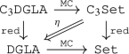  (3.13)

  commutes with $\eta$ injective.

• ii.) There exists a natural isomorphism $\eta :\texttt {red}\circ \texttt {G} \Longrightarrow \texttt {G} \circ \texttt {red}$, i.e.

  

  (3.14)

  commutes with $\eta$ injective.

• iii.) There exists an injective natural transformation $\eta :\texttt {red}\circ \texttt {Def}\Longrightarrow \texttt {Def}\circ \texttt {red}$, i.e.

  

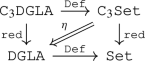  (3.15)

  commutes with $\eta$ injective.

Proof

• i.) In the following we denote by $[\,\cdot \,]_{\mathrm{MC}}$ the equivalence classes of elements in $\texttt {MC}(\mathfrak {g}_{\mathrm{N}})$ and by $[\,\cdot \,]_\mathfrak {g}$ the equivalence classes of elements in $\mathfrak {g}_{\mathrm{N}}$. For any coisotropic DGLA $\mathfrak {g}$ define $\eta _\mathfrak {g} :\texttt {MC}(\mathfrak {g})_\texttt {red}\rightarrow \texttt {MC}(\mathfrak {g}_\texttt {red})$ by $\eta _\mathfrak {g}([\xi ]_{\mathrm{MC}}) = [\xi ]_\mathfrak {g}$. This map is well-defined since $[\xi ]_{\mathrm{MC}}\subseteq [\xi ]_\mathfrak {g}$ and

  $$\begin{aligned} \mathop {}\!\mathrm {d}_\texttt {red}[\xi ]_\mathfrak {g} + \big [ [\xi ]_\mathfrak {g}, [\xi ]_\mathfrak {g} \big ]_\texttt {red}= \big [ \mathop {}\!\mathrm {d}_{\mathrm{N}}\xi + [\xi ,\xi ]_{\mathrm{N}}\big ]_\mathfrak {g} = [0]_\mathfrak {g} \end{aligned}$$

  for every $\xi \in \texttt {MC}(\mathfrak {g}_{\mathrm{N}})$. To show that $\eta _\mathfrak {g}$ is injective let $[\xi _1]_{\mathrm{MC}}, [\xi _2]_{\mathrm{MC}}\in \texttt {MC}(\mathfrak {g})_\texttt {red}$ be given such that $[\xi _1]_\mathfrak {g} = [\xi _2]_\mathfrak {g}$. Then $\xi _2 \in [\xi _1]_\mathfrak {g}$ and hence $\xi _1-\xi _2 \in \mathfrak {g}_{0}^1$. Thus by definition $\xi _1 \sim _{\mathrm{MC}}\xi _2$ and therefore $[\xi _1]_{\mathrm{MC}}= [\xi _2]_{\mathrm{MC}}$. To show naturality of $\eta$ let a morphism $\Phi :\mathfrak {g} \rightarrow \mathfrak {h}$ of coisotropic DGLAs be given. This induces morphisms $\Phi :\texttt {MC}(\mathfrak {g})_\texttt {red}\rightarrow \texttt {MC}(\mathfrak {h})_\texttt {red}$ and $\Phi :\texttt {MC}(\mathfrak {g}_\texttt {red}) \rightarrow \texttt {MC}(\mathfrak {h}_\texttt {red})$ by applying $\Phi _{\mathrm{N}}$ to representatives. Then we have

  $$\begin{aligned} (\eta _\mathfrak {h} \circ \Phi )([\xi ]_{\mathrm{MC}}) = \eta _\mathfrak {h}([\Phi _{\mathrm{N}}(\xi )]_{\mathrm{MC}}) = [\Phi _{\mathrm{N}}(\xi )]_\mathfrak {h} = \Phi ([\xi ]_\mathfrak {g}) = \Phi (\eta _\mathfrak {g}([\xi ]_{\mathrm{MC}})), \end{aligned}$$

  showing that $\eta$ is natural.

• ii.) Then $\eta _\mathfrak {g} :\texttt {G}(\mathfrak {g})_\texttt {red}\rightarrow \texttt {G}(\mathfrak {g}_\texttt {red})$ given by $[\lambda g]_{\texttt {G}}\mapsto \lambda [g]_\mathfrak {g}$, where $[g]_\mathfrak {g}$ denotes the equivalence class of g in $\mathfrak {g}_\texttt {red}$, is well-defined. Indeed, $\eta _\mathfrak {g}$ is just the $\lambda$-linear extension of the obvious identity $\mathfrak {g}_{\mathrm{N}}/ \mathfrak {g}_{0}= \mathfrak {g}_\texttt {red}$. Moreover, $\eta _\mathfrak {g}$ is a group morphism, since $[\,\cdot \,]_\mathfrak {g} :\mathfrak {g}_{\mathrm{N}}\rightarrow \mathfrak {g}_\texttt {red}$ is a morphism of DGLAs and $\bullet$ is given by sums of iterated brackets. Naturality follows directly.

• iii.) Let $\mathfrak {g} \in \texttt {C}_{3}{} \texttt {DGLA}$ be a coisotropic DGLA. Define $\eta _\mathfrak {g} :\texttt {Def}(\mathfrak {g})_\texttt {red}\rightarrow \texttt {Def}(\mathfrak {g}_\texttt {red})$ by $\left[ [\lambda g]_{\texttt {G}} \right] _\texttt {Def}\mapsto \left[ [\lambda g]_{\mathrm{MC}}\right] _{\texttt {G}}$ where $[\,\cdot \,]_{\texttt {G}}$ denotes the equivalence class induced by the action of the gauge group, $[\,\cdot \,]_\texttt {Def}$ denotes the equivalence class given by the equivalence relation on $\texttt {Def}(\mathfrak {g})_{\mathrm{N}}$ and $[\,\cdot \,]_{\mathrm{MC}}$ denotes the equivalence class given by the equivalence relation on $\texttt {MC}(\lambda \mathfrak {g}_\texttt {red}\llbracket \lambda \rrbracket )$. Now suppose that $[\lambda g']_{\texttt {G}}$ is another representative of $[[\lambda g]_{\texttt {G}}]_\texttt {Def}$, hence $\lambda g \sim _{\mathrm{MC}}\lambda g'$ by (3.11) and thus $\eta _\mathfrak {g}$ is well-defined. For the injectivity let $[[\lambda g ]_{\mathrm{MC}}]_{\texttt {G}} = [[\lambda g']_{\mathrm{MC}}]_{\texttt {G}}$ be given. Then $[\lambda g]_{\mathrm{MC}}= \lambda [h] \mathbin {\triangleright }[\lambda g']_{\mathrm{MC}}= [\lambda h \mathbin {\triangleright }_{\mathrm{N}}\lambda g' ]_{\mathrm{MC}}$ for some $[h] \in \mathfrak {g}_\texttt {red}\llbracket \lambda \rrbracket$ and therefore $[[\lambda g]_{\texttt {G}}]_\texttt {Def}= [[\lambda g']_{\texttt {G}}]_\texttt {Def}$. Naturality follows as above.

$\square$

4 Deformation theory of coisotropic algebras

4.1 Deformations of coisotropic algebras

In formal deformation quantization one is interested in algebras of formal power series over a ring $\mathbbm {k}\llbracket \lambda \rrbracket$, e.g. as algebra over ${\mathbb {C}}\llbracket \lambda \rrbracket$ for a Poisson manifold M with star product $\star$. For this reason, we consider deformations of a coisotropic algebra $\mathscr {A}$ with respect to the augmented (coisotropic) ring ${\underline{\mathbbm {k}}}\llbracket \lambda \rrbracket = (\mathbbm {k}\llbracket \lambda \rrbracket ,\mathbbm {k}\llbracket \lambda \rrbracket ,0)$. Given a coisotropic $\mathbbm {k}$-algebra $\mathscr {A} \in \texttt {C}_{3}{} \texttt {Alg}_{\underline{\mathbbm {k}}}$, we can define a formal deformation to be a coisotropic $\mathbbm {k}\llbracket \lambda \rrbracket$-algebra $\mathscr {B}$ together with an isomorphism $\alpha :\text {cl}(\mathscr {B}) \longrightarrow \mathscr {A}$. Here $\text {cl}(\mathscr {B})$ denotes the classical limit as introduced in [14]: The classical limit of a coisotropic $\mathbbm {k}\llbracket \lambda \rrbracket$-algebra $\mathscr {B}$ is the coisotropic $\mathbbm {k}$-algebra defined as $\text {cl}(\mathscr {B}) =\mathscr {B}/\lambda \mathscr {B} = (\mathscr {B}_\mathrm{tot}/\lambda \mathscr {B}_\mathrm{tot}, \mathscr {B}_{\mathrm{N}}/ \lambda \mathscr {B}_{\mathrm{N}}, \mathscr {B}_{0}/ \lambda \mathscr {B}_{\mathrm{N}})$. It is easy to see that this definition agrees with the one from deformation via Artin rings, see, e.g. [26]. Usually, one is interested in more specific deformations, namely those that are, e.g. free $\mathbbm {k}$-modules. This leads us to the following definition:

Definition 4.1

(Deformation of coisotropic algebra) Let $\mathscr {A} \in \texttt {C}_{3}{} \texttt {Alg}_{\underline{\mathbbm {k}}}$ be a coisotropic algebra. A (formal associative) deformation of $\mathscr {A}$ is given by an associative multiplication $\mu :\mathscr {A}\llbracket \lambda \rrbracket \otimes \mathscr {A}\llbracket \lambda \rrbracket \longrightarrow \mathscr {A}\llbracket \lambda \rrbracket$ on $\mathscr {A}\llbracket \lambda \rrbracket$ turning it into a coisotropic $\mathbbm {k}\llbracket \lambda \rrbracket$-algebra such that $\text {cl}(\mathscr {A}\llbracket \lambda \rrbracket ,\mu ) \simeq \mathscr {A}$.

Let us comment on this definition. First recall that we have

$$\begin{aligned} \mathscr {A}\llbracket \lambda \rrbracket = \left( \mathscr {A}_\mathrm{tot}\llbracket \lambda \rrbracket , \mathscr {A}_{\mathrm{N}}\llbracket \lambda \rrbracket , \mathscr {A}_{0}\llbracket \lambda \rrbracket \right) \end{aligned}$$

(4.1)

with the structure map $\iota _{\mathscr {A}\llbracket \lambda \rrbracket } = \iota _{\mathscr {A}}$ being just the $\lambda$-linear extension of the previous map according to (3.6). Then we have two formal associative deformations $\mu _\mathrm{tot}$ and $\mu _{\mathrm{N}}$ for $\mathscr {A}_\mathrm{tot}\llbracket \lambda \rrbracket$ and $\mathscr {A}_{\mathrm{N}}\llbracket \lambda \rrbracket$ of the form $\mu _\mathrm{tot}= (\mu _\mathrm{tot})_0 + \lambda (\mu _\mathrm{tot})_1 + \lambda ^2(\dotsc )$ and $\mu _{\mathrm{N}}= (\mu _{\mathrm{N}})_0 + \lambda (\mu _{\mathrm{N}})_1 + \lambda ^2(\dotsc )$, respectively, such that the undeformed map $\iota _{\mathscr {A}}$ is an algebra homomorphism and such that $\mathscr {A}_{0}\llbracket \lambda \rrbracket$ is a two-sided ideal in $\mathscr {A}_{\mathrm{N}}\llbracket \lambda \rrbracket$ with respect to $\mu _{\mathrm{N}}$. Note that we insist on the $\mathscr {A}_{\mathrm{N}}$ and $\mathscr {A}_{0}$ being the same up to taking formal series. Also the algebra morphism $\iota _{\mathscr {A}}$ is not deformed. There are various approaches to study the deformations of various kinds of algebras and their morphisms, e.g. via derived bracket as in [21] or with operadic approach as in [20]. Nevertheless, our goal is to deform the multiplicative structure of a coisotropic algebra, but not the morphism it contains.

One particular scenario we will be interested in the context of deformation quantization of phase space reduction is the following:

Example 4.2

For convenience, we will assume that $\mathbbm {k}$ is actually a field and not just a ring. Let $\mathscr {A} = (\mathscr {A}_\mathrm{tot}\supseteq \mathscr {A}_{\mathrm{N}}\supseteq \mathscr {A}_{0})$ be a coisotropic triple such that $\mathscr {A}_{0}\subseteq \mathscr {A}_\mathrm{tot}$ is a left ideal and $\mathscr {A}_{\mathrm{N}}\subseteq {\text {N}}(\mathscr {A}_{0})$ is a unital subalgebra of the normalizer of this left ideal. In particular, $\iota _{\mathscr {A}}$ is just the inclusion. Consider now a formal associative deformation $\mu _\mathrm{tot}$ of $\mathscr {A}_\mathrm{tot}$ with the additional property that the formal series $\mathscr {A}_{0}\llbracket \lambda \rrbracket$ are still a left ideal inside $\mathscr {A}_\mathrm{tot}\llbracket \lambda \rrbracket$ with respect to $\mu _\mathrm{tot}$. Moreover, assume that the normalizer ${\pmb {\mathscr {A}}}_{\mathrm{N}}= {\text {N}}_{\mu _\mathrm{tot}}(\mathscr {J}\llbracket \lambda \rrbracket ) \subseteq \mathscr {A}_\mathrm{tot}\llbracket \lambda \rrbracket$ with respect to $\mu _\mathrm{tot}$ satisfies

$$\begin{aligned} \text {cl}({\pmb {\mathscr {A}}}_{\mathrm{N}}) \subseteq \mathscr {A}_{\mathrm{N}}. \end{aligned}$$

(4.2)

This would be automatically true if $\mathscr {A}_{\mathrm{N}}$ coincides with the undeformed normalizer but poses an additional condition otherwise.

It is now easy to check that ${\pmb {\mathscr {A}}}_{\mathrm{N}}\subseteq \mathscr {A}_\mathrm{tot}\llbracket \lambda \rrbracket$ is a closed subspace with respect to the $\lambda$-adic topology. Moreover, if $\lambda a \in {\pmb {\mathscr {A}}}_{\mathrm{N}}$ for some $a \in \mathscr {A}_\mathrm{tot}\llbracket \lambda \rrbracket$ we can conclude $a \in {\pmb {\mathscr {A}}}\llbracket \lambda \rrbracket$. Hence ${\pmb {\mathscr {A}}}_{\mathrm{N}}\subseteq \mathscr {A}\llbracket \lambda \rrbracket$ is a deformation of a subspace in the sense of [6, Def. 30], i.e. we have a subspace $\mathscr {D} \subseteq \mathscr {A}_\mathrm{tot}$ and linear maps $q_r:\mathscr {D} \longrightarrow \mathscr {A}_\mathrm{tot}$ for $r \in {\mathbb {N}}$ such that

$$\begin{aligned} {\pmb {\mathscr {A}}}_{\mathrm{N}}= q (\mathscr {D}\llbracket \lambda \rrbracket ) \end{aligned}$$

(4.3)

where $q = \iota _{\mathscr {D}} + \sum _{r=1}^\infty \lambda ^r q_r$ with $\iota _{\mathscr {D}}$ being the canonical inclusion of the subspace. By our assumption, $\mathscr {D} \subseteq \mathscr {A}_{\mathrm{N}}$ but the inclusion could be proper. Moreover, since by our assumption $\mathscr {A}_{0}\llbracket \lambda \rrbracket \subseteq {\text {N}}(\mathscr {A}_{0}\llbracket \lambda \rrbracket ) = {\pmb {\mathscr {A}}}_{\mathrm{N}}$, we have $\mathscr {A}_{0}\subseteq \mathscr {D}$.

Since we work over a field, we can find a complement $\mathscr {C} \subseteq \mathscr {D}$ such that $\mathscr {A}_{0}\oplus \mathscr {C} = \mathscr {D}$. This allows to redefine the maps $q_r$ to

$$\begin{aligned} q'_r\big |_{\mathscr {C}} = q_r\big |_{\mathscr {C}} \quad \text{ and } \quad q'_r\big |_{\mathscr {A}_{0}} = 0. \end{aligned}$$

(4.4)

The resulting map $q'$ then satisfies $q'(\mathscr {D}\llbracket \lambda \rrbracket ) = {\pmb {\mathscr {A}}}_{\mathrm{N}}$ and $q'\big |_{\mathscr {A}_{0}} = \text{ id}_{\mathscr {A}_{0}}$. We can then use $q'$ to pass to a new deformation $\mu '_\mathrm{tot}$ of $\mathscr {A}_\mathrm{tot}$ with the property that $\mathscr {A}_{0}\llbracket \lambda \rrbracket$ is still a left ideal in $\mathscr {A}_\mathrm{tot}\llbracket \lambda \rrbracket$ with respect to $\mu '_\mathrm{tot}$ and the normalizer of this left ideal is now given by $\mathscr {D}\llbracket \lambda \rrbracket \subseteq \mathscr {A}_\mathrm{tot}\llbracket \lambda \rrbracket$. It follows that $\mu '_\mathrm{tot}$ provides a deformation of the coisotropic triple $(\mathscr {A}_\mathrm{tot}, \mathscr {D}, \mathscr {A}_{0})$ in the sense of Definition 4.1.

Of course, it might happen that $\mathscr {D} \ne \mathscr {A}_{\mathrm{N}}$ and hence this construction will not provide a deformation of the original coisotropic triple, in general. It turns out that this can be controlled as follows: we assume in addition that the deformed normalizer ${\pmb {\mathscr {A}}}_{\mathrm{N}}$ is large enough in the sense that the classical limit

$$\begin{aligned} \text {cl}:{\pmb {\mathscr {A}}}_\texttt {red}= {\pmb {\mathscr {A}}}_{\mathrm{N}}\big / (\mathscr {A}_{0}\llbracket \lambda \rrbracket ) \longrightarrow \mathscr {A}_\texttt {red}= \mathscr {A}_{\mathrm{N}}\big / \mathscr {A}_{0}\end{aligned}$$

(4.5)

between the reduced algebras is surjective. As $\mathbbm {k}$ is a field, this gives us a split $Q:\mathscr {A}_\texttt {red}\longrightarrow {\pmb {\mathscr {A}}}_\texttt {red}$ which we can extend $\lambda$-linearly to

$$\begin{aligned} Q:\mathscr {A}_\texttt {red}\llbracket \lambda \rrbracket \longrightarrow {\pmb {\mathscr {A}}}_\texttt {red}. \end{aligned}$$

(4.6)

It is then easy to see that this is in fact a $\mathbbm {k}\llbracket \lambda \rrbracket$-linear isomorphism. It follows, that in this case we necessarily have

$$\begin{aligned} \mathscr {D} = \mathscr {A}_{\mathrm{N}}. \end{aligned}$$

(4.7)

Thus the previous construction gives indeed a deformation $\mu '_\mathrm{tot}$ of the original coisotropic triple. This seemingly very special situation will turn out to be responsible for one of the main examples from deformation quantization.

4.2 Coisotropic Hochschild cohomology

From now on we assume that $\mathbbm {Q} \subseteq \mathbbm {k}$. Let $\mathscr {M}, \mathscr {N} \in \texttt {C}_{3}{} \texttt {Mod}_{\underline{\mathbbm {k}}}$ be coisotropic modules. We define for any $n \in {\mathbb {N}}$

$$\begin{aligned} \text {C}^n(\mathscr {M}, \mathscr {N}) = \texttt {C}_{3}{} \texttt {Hom}_{\underline{\mathbbm {k}}}(\mathscr {M}^{\otimes n},\mathscr {N}) \end{aligned}$$

(4.8)

with $\texttt {C}_{3}{} \texttt {Hom}_{\underline{\mathbbm {k}}}$ denoting the internal Hom as usual. Recall that

$$\begin{aligned} \text {C}^n(\mathscr {M},\mathscr {N})_\mathrm{tot}&= \text {Hom}_\mathbbm {k}(\mathscr {M}_\mathrm{tot}^{\otimes n}, \mathscr {N}_\mathrm{tot}), \\ \text {C}^n(\mathscr {M},\mathscr {N})_{\mathrm{N}}&= \text {Hom}_{\underline{\mathbbm {k}}}(\mathscr {M}^{\otimes n},\mathscr {N}), \\ \text {C}^n(\mathscr {M},\mathscr {N})_{0}&= \big \{ (f_\mathrm{tot},f_{\mathrm{N}}) \in \text {C}^n(\mathscr {M}^{\otimes n},\mathscr {N}) \; \big | \; f_{\mathrm{N}}(\mathscr {M}^{\otimes n}_{\mathrm{N}}) \subseteq \mathscr {N}_{0}\big \} \end{aligned}$$

with $\iota _n :\text {C}^n(\mathscr {M},\mathscr {N})_{\mathrm{N}}\ni (f_\mathrm{tot},f_{\mathrm{N}}) \mapsto f_\mathrm{tot}\in \text {C}^n(\mathscr {M},\mathscr {N})_\mathrm{tot}$. Note that a morphism $f = (f_\mathrm{tot}, f_{\mathrm{N}}) \in \text {C}^n(\mathscr {M},\mathscr {N})_{\mathrm{N}}$ fulfils $f_{\mathrm{N}}((\mathscr {M}^{\otimes n})_{0}) \subseteq \mathscr {N}_{0}$ where, by definition of the tensor product, we have

$$\begin{aligned} (\mathscr {M}^{\otimes n})_{0}= \sum _{i=1}^{n} \mathscr {M}^{\otimes i-1}_{\mathrm{N}}\otimes \mathscr {M}_{0}\otimes \mathscr {M}_{\mathrm{N}}^{\otimes n-i}. \end{aligned}$$

(4.9)

In other words, $f_{\mathrm{N}}$ maps to $\mathscr {N}_{0}$ if at least one tensor factor comes from $\mathscr {M}_{0}$. This clearly defines a graded coisotropic $\mathbbm {k}$-module $\text {C}^\bullet (\mathscr {M},\mathscr {N})$.

Let us now consider the case $\mathscr {N} = \mathscr {M}$. Then we write $\text {C}^\bullet (\mathscr {M}) = \text {C}^\bullet (\mathscr {M},\mathscr {M})$. We now want to transfer the Gerstenhaber algebra structure of the classical Hochschild complex to $\text {C}^\bullet (\mathscr {M})$. For this denote by $[\,\cdot \,,\,\cdot \,]^{\mathscr {M}_\mathrm{tot}}$ and $[\,\cdot \,,\,\cdot \,]^{\mathscr {M}_{\mathrm{N}}}$ the Gerstenhaber brackets for the modules $\mathscr {M}_\mathrm{tot}$ and $\mathscr {M}_{\mathrm{N}}$, respectively. Then we need to show that $[\,\cdot \,,\,\cdot \,]^{\mathscr {M}_{\mathrm{N}}}$ preserves the $0$-components. This follows directly from the usual formula for the Gerstenhaber bracket, see [22].

Definition 4.3

(Gerstenhaber bracket) Let $\mathscr {M} \in \texttt {C}_{3}{} \texttt {Mod}_{\underline{\mathbbm {k}}}$. Then the morphism $[\,\cdot \,, \,\cdot \,] :\text {C}^\bullet (\mathscr {M}) \otimes \text {C}^\bullet (\mathscr {M}) \rightarrow \text {C}^\bullet (\mathscr {M})$ of coisotropic $\mathbbm {k}$-modules defined by

$$\begin{aligned}{}[\,\cdot \,, \,\cdot \,]_\mathrm{tot}= [\,\cdot \,,\,\cdot \,]^{\mathscr {M}_\mathrm{tot}} \quad \text { and }\quad [\,\cdot \,, \,\cdot \,]_{\mathrm{N}}=\big ([\,\cdot \,,\,\cdot \,]^{\mathscr {M}_\mathrm{tot}}, [\,\cdot \,,\,\cdot \,]^{\mathscr {M}_{\mathrm{N}}}\big ) \end{aligned}$$

(4.10)

is called the coisotropic Gerstenhaber bracket.

Since $[\,\cdot \,, \,\cdot \,]^{\mathscr {M}_\mathrm{tot}}$ and $[\,\cdot \,, \,\cdot \,]^{\mathscr {M}_{\mathrm{N}}}$ induce graded Lie algebra structures on the classical Hochschild complexes of $\mathscr {M}_\mathrm{tot}$ and $\mathscr {M}_{\mathrm{N}}$ it is easy to see that $\text {C}^\bullet (\mathscr {M})$ together with the coisotropic Gerstenhaber bracket $[\,\cdot \,, \,\cdot \,]$ forms a graded coisotropic Lie algebra.

Remark 4.4

The coisotropic Gerstenhaber bracket can also be derived from a coisotropic pre-Lie algebra structure on $\text {C}^\bullet (\mathscr {M})$, which in turn results from a sort of partial composition. These partial compositions can be interpreted as the usual endomorphism operad structure of $\mathscr {M}$ in $\texttt {C}_{3}{} \texttt {Mod}_{\underline{\mathbbm {k}}}$. The theory of operads in the (non-abelian) category $\texttt {C}_{3}{} \texttt {Mod}_{\underline{\mathbbm {k}}}$ will be the subject of a future project.

As in the standard theory of deformation of associative algebras, we can characterize associative multiplications by using the Gerstenhaber bracket.

Lemma 4.5

Let $\mathscr {M} \in \texttt {C}_{3}{} \texttt {Mod}_{\underline{\mathbbm {k}}}$ be a coisotropic module. Then a morphism $\mu :\mathscr {M} \otimes \mathscr {M} \longrightarrow \mathscr {M}$ of coisotropic $\mathbbm {k}$-modules is an associative coisotropic algebra structure on $\mathscr {M}$ if and only if

$$\begin{aligned}{}[\mu , \mu ]_{\mathrm{N}}= 0. \end{aligned}$$

(4.11)

Proof

First, note that a coisotropic morphism $\mu :\mathscr {M} \otimes \mathscr {M} \rightarrow \mathscr {M}$ is an element in $\text {C}^2(\mathscr {M})_{\mathrm{N}}$ and hence consists of a pair $(\mu _\mathrm{tot}, \mu _{\mathrm{N}})$ and $[\,\cdot \,, \,\cdot \,]_{\mathrm{N}}= ([\,\cdot \,, \,\cdot \,]^{\mathscr {M}_\mathrm{tot}}, [\,\cdot \,,\,\cdot \,]^{\mathscr {M}_{\mathrm{N}}})$. From the classical theory for associative algebras we know that $\mu _\mathrm{tot}$ and $\mu _{\mathrm{N}}$ are associative multiplications if and only if $[\mu _\mathrm{tot},\mu _\mathrm{tot}]^{\mathscr {M}_\mathrm{tot}} = 0$ and $[\mu _{\mathrm{N}}, \mu _{\mathrm{N}}]^{\mathscr {M}_{\mathrm{N}}} = 0$ holds. $\square$

Note that (4.11) only involves the ${\text {N}}$-component of the coisotropic Gerstenhaber bracket $[\,\cdot \,, \,\cdot \,]$. Using the coisotropic structure of $\text {C}^2(\mathscr {M})$ we get $\iota _2(\mu ) = \mu _\mathrm{tot}\in \text {C}^2(\mathscr {M})_\mathrm{tot}$, from which directly $[\mu _\mathrm{tot},\mu _\mathrm{tot}]_\mathrm{tot}= 0$ follows.

Let us now move from a module $\mathscr {M}$ to an algebra $(\mathscr {A},\mu )$. Then we can use the multiplication to construct a differential on $\text {C}^\bullet (\mathscr {A})$.

Proposition 4.6

(Coisotropic Hochschild differential) Let $(\mathscr {A}, \mu ) \in \texttt {C}_{3}{} \texttt {Alg}_{\underline{\mathbbm {k}}}$ be a coisotropic algebra. Then the morphism $\delta :\text {C}^\bullet (\mathscr {A}) \rightarrow \text {C}^{\bullet +1}(\mathscr {A})$ of coisotropic $\mathbbm {k}$-modules, defined by its components

$$\begin{aligned} \delta _\mathrm{tot}= -[\,\cdot \,, \mu _\mathrm{tot}]_\mathrm{tot}\quad \text { and } \quad \delta _{\mathrm{N}}= -[\,\cdot \,, \mu ]_{\mathrm{N}}, \end{aligned}$$

(4.12)

is a coisotropic chain map of degree 1 and $\delta ^2 = 0$.

Proof

Since $\mu _\mathrm{tot}$ is an associative multiplication on $\mathscr {A}_\mathrm{tot}$ we know that $\delta _\mathrm{tot}:\text {C}^\bullet (\mathscr {A}_\mathrm{tot}) \longrightarrow \text {C}^{\bullet +1}(\mathscr {A}_\mathrm{tot})$ is a differential. Moreover, it is clear that $\delta _{\mathrm{N}}:\text {C}^\bullet (\mathscr {A})_{\mathrm{N}}\longrightarrow \text {C}^\bullet (\mathscr {A})_{\mathrm{N}}$ is also a differential and it preserves the $0$-component by the definition of $[\,\cdot \,, \,\cdot \,]_{\mathrm{N}}$. Finally, we have for $(\Phi _\mathrm{tot},\Phi _{\mathrm{N}}) \in \text {C}^n(\mathscr {A})_{\mathrm{N}}$ that $(\delta _\mathrm{tot}\circ \iota _n)(\Phi _\mathrm{tot},\Phi _{\mathrm{N}}) = \delta _\mathrm{tot}(\Phi _\mathrm{tot}) = \iota _{n+1}(\delta _{\mathrm{N}}((\Phi _\mathrm{tot},\Phi _{\mathrm{N}})))$ holds, and hence $(\delta _\mathrm{tot},\delta _{\mathrm{N}})$ is a coisotropic morphism. $\square$

Note that $\delta _{\mathrm{N}}$ can be seen as a coevaluation morphism according to Sect. 2.1m). The coisotropic Hochschild differential can be interpreted as twisting the coisotropic DGLA $(\text {C}^\bullet (\mathscr {A}), [\,\cdot \,, \,\cdot \,],0)$ with the Maurer–Cartan element $\mu \in \text {C}^2(\mathscr {A})_{\mathrm{N}}$, but with signs chosen in such a way that it corresponds to the usual Hochschild differential. More explicitly we have the following result.

Corollary 4.7

Let $(\mathscr {A},\mu ) \in \texttt {C}_{3}{} \texttt {Alg}_{\underline{\mathbbm {k}}}$ be a coisotropic algebra. Then the coisotropic Hochschild differential $\delta :\text {C}^\bullet (\mathscr {A}) \longrightarrow \text {C}^{\bullet +1}(\mathscr {A})$ is given by $\delta = (\delta ^{\mathscr {A}_\mathrm{tot}}, (\delta ^{\mathscr {A}_\mathrm{tot}},\delta ^{\mathscr {A}_{\mathrm{N}}}))$, where $\delta ^{\mathscr {A}_\mathrm{tot}}$ and $\delta ^{\mathscr {A}_{\mathrm{N}}}$ denote the Hochschild differentials of the algebras $(\mathscr {A}_\mathrm{tot}, \mu _\mathrm{tot})$ and $(\mathscr {A}_{\mathrm{N}}, \mu _{\mathrm{N}})$, respectively.

From this explicit characterization of the coisotropic Hochschild differential in terms of the classical Hochschild differentials it becomes clear that $(\text {C}^\bullet (\mathscr {A}),[\,\cdot \,,\,\cdot \,],\delta )$ is a coisotropic DGLA.

Definition 4.8

(Coisotropic Hochschild complex) Let $(\mathscr {A},\mu ) \in \texttt {C}_{3}{} \texttt {Alg}_{\underline{\mathbbm {k}}}$ be a coisotropic algebra. The coisotropic DGLA $(\text {C}^\bullet (\mathscr {A}),[\,\cdot \,,\,\cdot \,],\delta )$ is called the coisotropic Hochschild complex of $\mathscr {A}$.

Assigning the (coisotropic) Hochschild complex to a given (coisotropic) algebra is not functorial on all of $\texttt {C}_{3}{} \texttt {Alg}_{\underline{\mathbbm {k}}}$. But if we restrict ourselves to the subcategory $\texttt {C}_{3}{} \texttt {Alg}_{\underline{\mathbbm {k}}}^\times$ of coisotropic algebras with invertible morphisms we get a functor $\text {C}^\bullet :\texttt {C}_{3}{} \texttt {Alg}_{\underline{\mathbbm {k}}}^\times \rightarrow \texttt {C}_{3}{} \texttt {DGLA}$ by mapping each coisotropic algebra to its coisotropic Hochschild complex and every algebra isomorphism $\phi :\mathscr {A} \rightarrow \mathscr {B}$ to $\text {C}^\bullet (\phi ) :\text {C}^\bullet (\mathscr {A}) \rightarrow \text {C}^\bullet (\mathscr {B})$ given by $\text {C}^\bullet (\phi )(f) = \phi \circ f \circ (\phi ^{-1})^{\otimes n}$ for $f \in \text {C}^n(\mathscr {A})_{\mathrm{tot}/{\mathrm{N}}}$. A similar construction clearly also works for usual algebras. We can now show that this functor commutes with reduction up to an injective natural transformation.

Proposition 4.9

(Hochschild complex versus reduction) There exists an injective natural transformation $\eta :\texttt {red}\circ \text {C}^\bullet \Longrightarrow \text {C}^\bullet \circ \texttt {red}$, i.e.

(4.13)

commutes.

Proof

For every coisotropic algebra $\mathscr {A}$ define $\eta _\mathscr {A} :\text {C}^\bullet (\mathscr {A})_\texttt {red}\rightarrow \text {C}^\bullet (\mathscr {A}_\texttt {red})$ by

$$\begin{aligned} \eta _\mathscr {A}([f])([a_1], \dotsc , [a_n]) = \left[ f_{\mathrm{N}}(a_1, \dotsc , a_n) \right] . \end{aligned}$$

for $[f]=[(f_\mathrm{tot},f_{\mathrm{N}})] \in \text {C}^n(\mathscr {A})_\texttt {red}$. First note that $\eta _\mathscr {A}([f]) :\mathscr {A}_\texttt {red}^{\otimes n} \rightarrow \mathscr {A}_\texttt {red}$ is well defined since if $a_i \in \mathscr {A}_0$ for any $i = 1,\dotsc ,n$ we have $f_{\mathrm{N}}(a_1, \dotsc , a_n) \in \mathscr {A}_{0}$ and hence $[f_{\mathrm{N}}(a_1, \dotsc , a_n)] = 0$. Moreover, $\eta _\mathscr {A}$ is well-defined since for $f \in \text {C}^n(\mathscr {A})_{0}$ we have $f_{\mathrm{N}}(a_1, \dotsc , a_n) \in \mathscr {A}_{0}$ and thus $\eta ([f]) = 0$. To see that $\eta$ is indeed a natural transformation we need to show that for every isomorphism $\phi :\mathscr {A} \rightarrow \mathscr {B}$ we have $\eta _\mathscr {B} \circ \text {C}^\bullet (\phi )_\texttt {red}= \text {C}^\bullet ([\phi ]) \circ \eta _\mathscr {A}$. But it is clear after inserting the definitions. Finally, suppose $\eta _\mathscr {A}([f]) = \eta _\mathscr {A}([g])$. This means that $(f_{\mathrm{N}}-g_{\mathrm{N}})(a_1, \dotsc , a_n) \in \mathscr {A}_{0}$ and therefore $[f] = [g]$. Thus $\eta _\mathscr {A}$ is injective. $\square$

Now let us turn to the cohomology of the coisotropic Hochschild complex.

Definition 4.10

(Coisotropic Hochschild cohomology) Let $(\mathscr {A},\mu ) \in \texttt {C}_{3}{} \texttt {Alg}_{\underline{\mathbbm {k}}}$ be a coisotropic algebra. The cohomology $\texttt {HH}^\bullet (\mathscr {A}) = \ker \delta / \text {im}\delta$ of the Hochschild complex $\text {C}^\bullet (A)$ is called the coisotropic Hochschild cohomology of $\mathscr {A}$.

Using the definition of kernel, image and quotient in $\texttt {C}_{3}{} \texttt {Mod}_{\underline{\mathbbm {k}}}$ as given in Sect. 2.1e, g, j we can express the coisotropic Hochschild cohomology more explicitly as follows.

Lemma 4.11

The coisotropic Hochschild cohomology of $\mathscr {A} \in \texttt {C}_{3}{} \texttt {Alg}_{\underline{\mathbbm {k}}}$ is given by

$$\begin{aligned} \texttt {HH}^\bullet (\mathscr {A})_\mathrm {tot}&= \texttt {HH}^\bullet (\mathscr {A}_\mathrm {tot}), \end{aligned}$$

(4.14)

$$\begin{aligned} \texttt {HH}^\bullet (\mathscr {A})_{\mathrm {N}}&= \ker \delta _{\mathrm {N}}/ \text{ im }\delta _{\mathrm {N}}, \text {and} \end{aligned}$$

(4.15)

$$\begin{aligned} \texttt {HH}^\bullet (\mathscr {A})_{0}&= \ker (\delta _{\mathrm {N}}\big |_{{0}}) / \text{ im }\delta _{\mathrm {N}} \end{aligned}$$

(4.16)

with

$$\begin{aligned} \ker \delta _{\mathrm{N}}^{n+1}&= \big \{ (f_\mathrm{tot}, f_{\mathrm{N}}) \in \text {C}^{n+1}(\mathscr {A})_{\mathrm{N}}\; \big | \; \delta ^{\mathscr {A}_\mathrm{tot}} f_\mathrm{tot}= 0 \text { and } \delta ^{\mathscr {A}_{\mathrm{N}}} f_{\mathrm{N}}= 0 \big \} \subseteq \ker \delta _{\mathscr {A}_\mathrm{tot}}^{n+1} \times \ker \delta _{\mathscr {A}_{\mathrm{N}}}^{n+1}, \end{aligned}$$

(4.17)

$$\begin{aligned} \text {im}\delta _{\mathrm{N}}^n&= \big \{ (f_\mathrm{tot}, f_{\mathrm{N}}) \in \text {C}^{n+1}(\mathscr {A})_{\mathrm{N}}\; \big | \; \exists (g_\mathrm{tot}, g_{\mathrm{N}}) \in \text {C}^n(\mathscr {A})_{\mathrm{N}}: \delta ^{\mathscr {A}_\mathrm{tot}}g_\mathrm{tot}= f_\mathrm{tot}\text { and } \delta ^{\mathscr {A}_{\mathrm{N}}}g_{\mathrm{N}}= f_{\mathrm{N}}\big \}, \text {and} \end{aligned}$$

(4.18)

$$\begin{aligned} \ker (\delta ^n_{\mathrm {N}}\big |_{{0}} )&= \big \{ (f_\mathrm {tot}, f_{\mathrm {N}}) \in \text{ C}^{n+1}(\mathscr {A})_{0}\; \big | \; \delta ^{\mathscr {A}_\mathrm {tot}} f_\mathrm {tot}= 0 \text{ and } \delta ^{\mathscr {A}_{\mathrm {N}}} f_{\mathrm {N}}= 0 \big \} \subseteq \ker \delta _{\mathscr {A}_\mathrm {tot}}^n \times \ker \delta _{\mathscr {A}_{\mathrm {N}}}^n. \end{aligned}$$

(4.19)

With this we can compute the zeroth and first coisotropic Hochschild cohomology of a given coisotropic algebra. The following also shows that in low degrees the interpretation of the coisotropic Hochschild cohomology is analogous to that for usual algebras.

Proposition 4.12

Let $\mathscr {A} \in \texttt {C}_{3}{} \texttt {Alg}_{\underline{\mathbbm {k}}}$ be a coisotropic algebra.

• i.) We have

  $$\begin{aligned} \texttt {HH}^0(\mathscr {A})_\mathrm{tot}&= \mathscr {Z}(\mathscr {A}_\mathrm{tot}), \end{aligned}$$

  (4.20)
  $$\begin{aligned} \texttt {HH}^0(\mathscr {A})_{\mathrm{N}}&= \big \{ a \in \mathscr {A}_{\mathrm{N}}\; \big | \; a \in \mathscr {Z}(\mathscr {A}_{\mathrm{N}}) \text { and } \iota _\mathscr {A}(a) \in \mathscr {Z}(\mathscr {A}_\mathrm{tot}) \big \}, \text {and} \end{aligned}$$

  (4.21)
  $$\begin{aligned} \texttt {HH}^0(\mathscr {A})_{0}&= \big \{ a_0 \in \mathscr {A}_{0}\; \big | \; a_0 \in \mathscr {Z}(\mathscr {A}_{\mathrm{N}}) \text { and } \iota _\mathscr {A}(a_0) \in \mathscr {Z}(\mathscr {A}_\mathrm{tot}) \big \}. \end{aligned}$$

  (4.22)

• ii.) We have

  $$\begin{aligned} \texttt {HH}^1(\mathscr {A})_\mathrm{tot}&= \texttt {Der}(\mathscr {A}_\mathrm{tot}) / \texttt {InnDer}(\mathscr {A}_\mathrm{tot}), \end{aligned}$$

  (4.23)
  $$\begin{aligned} \texttt {HH}^1(\mathscr {A})_{\mathrm{N}}&= \texttt {Der}(\mathscr {A})_{\mathrm{N}}/ \big \{ (D_\mathrm{tot}, D_{\mathrm{N}}) \in \texttt {Der}(\mathscr {A})_{\mathrm{N}}\; \big | \; \exists a \in \mathscr {A}_{\mathrm{N}}: D_\mathrm{tot}= [\,\cdot \,, \iota _\mathscr {A}(a)], D_{\mathrm{N}}= [\,\cdot \,, a] \big \}, \text {and} \end{aligned}$$

  (4.24)
  $$\begin{aligned} \texttt {HH}^1(\mathscr {A})_{0}&= \texttt {Der}(\mathscr {A})_{0}/ \big \{ (D_\mathrm{tot}, D_{\mathrm{N}}) \in \texttt {Der}(\mathscr {A})_{\mathrm{N}}\; \big | \; \exists a \in \mathscr {A}_{\mathrm{N}}: D_\mathrm{tot}= [\,\cdot \,, \iota _\mathscr {A}(a)], D_{\mathrm{N}}= [\,\cdot \,, a] \big \}. \end{aligned}$$

  (4.25)

  Hence $\texttt {HH}^1(\mathscr {A}) = \texttt {C}_{3}\!\texttt {Der}(\mathscr {A}) / \texttt {C}_{3}\!\texttt {InnDer}(\mathscr {A})$.

Proof

The first claim is clear by Lemma 4.11 and $\delta _{-1} = 0$. The $\text {tot}$-component of the second part is clear by the classical result for the first Hochschild cohomology of the classical algebra $\mathscr {A}_\mathrm{tot}$. For the ${\text {N}}$-component consider $D = (D_\mathrm{tot},D_{\mathrm{N}}) \in \ker \delta _{\mathrm{N}}^1$. Then $\delta ^{\mathscr {A}_\mathrm{tot}}D_\mathrm{tot}= 0$ and $\delta ^{\mathscr {A}_{\mathrm{N}}}D_{\mathrm{N}}= 0$, hence $D_\mathrm{tot}$ and $D_{\mathrm{N}}$ are derivations and it follows $D \in \texttt {Der}(\mathscr {A})_{\mathrm{N}}$. Similarly, we get $D \in \texttt {Der}(\mathscr {A})_{0}$ for $D \in \ker (\delta _{\mathrm {N}}^1\big |_{{0}})$. Now let $D \in \text {im}\delta _{\mathrm{N}}^0$, then there exists $a :{\underline{\mathbbm {k}}} \rightarrow \mathscr {A}$ with $D_\mathrm{tot}= \delta ^{\mathscr {A}_\mathrm{tot}}a_\mathrm{tot}= [\,\cdot \,, a_\mathrm{tot}]$ and $D_{\mathrm{N}}= \delta ^{\mathscr {A}_{\mathrm{N}}}a_{\mathrm{N}}= [\,\cdot \,, a_{\mathrm{N}}]$. Since $a_\mathrm{tot}= \iota (a_{\mathrm{N}})$ the second part holds. $\square$

Remark 4.13

The center of a coisotropic algebra could now be defined as $\mathscr {Z}(\mathscr {A}) := \texttt {HH}^0(\mathscr {A})$. Similarly, one can define the outer derivations of a coisotropic algebra by $\text {OutDer}(\mathscr {A}) := \texttt {HH}^1(\mathscr {A})$.

Remark 4.14

Using methods from enriched category theory one can define the center of a monoid A internal to a given monoidal category $\mathfrak {C}$ by $[\mathfrak {C}, \mathfrak {C}](\text {id}_A, \text {id}_A)$. Here $[\mathfrak {C},\mathfrak {C}]$ denotes the $\mathfrak {C}$-enriched functor category of endofunctors of $\mathfrak {C}$. Applying this to the monoidal category $\texttt {C}_{3}{} \texttt {Mod}_{\underline{\mathbbm {k}}}$ yields exactly the notion of center of a coisotropic algebra as introduced in Remark 4.13.

Remark 4.15

Combining Proposition 2.21 with Proposition 4.9 immediately shows that there exists an injective natural transformation $\eta :\texttt {red}\circ \texttt {HH}^\bullet \Longrightarrow \texttt {HH}^\bullet \circ \texttt {red}$. In particular, for any coisotropic algebra $\mathscr {A}$ we have

$$\begin{aligned} \texttt {HH}^\bullet (\mathscr {A})_\texttt {red}\subseteq \texttt {HH}^\bullet (\mathscr {A}_\texttt {red}). \end{aligned}$$

(4.26)

Remark 4.16

In this section we defined the coisotropic Hochschild cohomology of coisotropic algebras only with the algebra itself as coefficients. It should be clear that all the above constructions also work for a coisotropic $\mathscr {A}$-bimodule $\mathscr {M}$ by using $\text {C}^\bullet (\mathscr {A},\mathscr {M})$.

4.3 Formal deformations

Throughout this section we will assume that the scalars satisfy $\mathbbm {Q} \subseteq \mathbbm {k}$ in order to make use of the description of deformations by Maurer–Cartan elements.

Let $(\mathscr {A},\mu _0) \in \texttt {C}_{3}{} \texttt {Alg}_{\underline{\mathbbm {k}}}$ be a coisotropic associative $\mathbbm {k}$-algebra. By Definition 4.1 a formal associative deformation $(\mathscr {A}\llbracket \lambda \rrbracket ,\mu )$ is given by an associative multiplication $\mu :\mathscr {A}\llbracket \lambda \rrbracket \otimes \mathscr {A}\llbracket \lambda \rrbracket \longrightarrow \mathscr {A}\llbracket \lambda \rrbracket$ making $\mathscr {A}\llbracket \lambda \rrbracket$ a coisotropic $\mathbbm {k}\llbracket \lambda \rrbracket$-algebra such that $\text {cl}(\mathscr {A},\mu )$ is given by $(\mathscr {A},\mu _0)$, or in other words

$$\begin{aligned} \mu = \mu _0 + \sum _{k=1}^{\infty } \lambda ^k \mu _k \end{aligned}$$

(4.27)

with $\mu _k :\mathscr {A} \otimes \mathscr {A} \rightarrow \mathscr {A}$. Such deformations can now be understood as Maurer–Cartan elements in the coisotropic DGLA $\lambda \text {C}^\bullet (\mathscr {A})\llbracket \lambda \rrbracket$ corresponding to $(\mathscr {A}\llbracket \lambda \rrbracket ,\mu _0)$.

Lemma 4.17

Let $(\mathscr {A},\mu ) \in \texttt {C}_{3}{} \texttt {Alg}_{\underline{\mathbbm {k}}}$ be a coisotropic associative $\mathbbm {k}$-algebra. A multiplication $\mu = \mu _0 + M$, with $M = \sum _{k=1}^{\infty } \lambda ^k \mu _k$ is a formal associative deformation of $\mu _0$ if and only if

$$\begin{aligned} \delta M + \frac{1}{2}[M, M] = 0. \end{aligned}$$

(4.28)

Proof

By Lemma 4.5 we know that we have to check that $[\mu _\mathrm{tot}, \mu _\mathrm{tot}]_{\mathscr {A}_\mathrm{tot}} = 0$ and $[\mu _{\mathrm{N}}, \mu _{\mathrm{N}}]_{\mathscr {A}_{\mathrm{N}}} = 0$. Thus, consider the total component of $\mu$ as $\mu _\mathrm{tot}= (\mu _0)_\mathrm{tot}+ M_\mathrm{tot}$. We have

$$\begin{aligned}{}[\mu _\mathrm{tot}, \mu _\mathrm{tot}] = [(\mu _0)_\mathrm{tot}+ M_\mathrm{tot}, (\mu _0)_\mathrm{tot}+ M_\mathrm{tot}] = 2 \delta M_\mathrm{tot}+ [M_\mathrm{tot}, M_\mathrm{tot}], \end{aligned}$$

where we used the associativity of $(\mu _0)_\mathrm{tot}$ and the graded skew-symmetry of Gerstenhaber bracket. The very same holds for the ${\text {N}}$-component. $\square$

Let us now consider two formal associative deformations $\mu$ and $\mu '$ of $(\mathscr {A},\mu _0)$. We say that they are equivalent if there exists $T = \text {id}+ \lambda (\ldots ) \in \texttt {C}_{3}\!\texttt {Aut}_{{\underline{\mathbbm {k}}}\llbracket \lambda \rrbracket }(\mathscr {A}\llbracket \lambda \rrbracket )$ such that $T \circ \mu = \mu ' \circ (T \otimes T)$, i.e. we have

$$\begin{aligned} T_\mathrm{tot}(\mu _\mathrm{tot}(a,b)) = \mu '_\mathrm{tot}(T_\mathrm{tot}(a), T_\mathrm{tot}(b)) \quad \text {and} \quad T_{\mathrm{N}}(\mu _{\mathrm{N}}(a,b)) = \mu '_{\mathrm{N}}(T_{\mathrm{N}}(a), T_{\mathrm{N}}(b))\nonumber \\ \end{aligned}$$

(4.29)

for $a, b \in \mathscr {A}_{\mathrm{tot}/{\mathrm{N}}}$. Thus, as in the case of associative algebras, there exists a unique $D = \sum _{k=0}^\infty \lambda ^k D_k \in \texttt {C}_{3}{} \texttt {Hom}_{\underline{\mathbbm {k}}}(\mathscr {A}\llbracket \lambda \rrbracket , \mathscr {A}\llbracket \lambda \rrbracket )$ such that $T = \exp (\lambda D)$. This allows us to conclude the following claim.

Lemma 4.18

Two formal associative deformations $\mu$ and $\mu '$ of a coisotropic $\mathbbm {k}$-algebra $(\mathscr {A},\mu _0)$ are equivalent if and only if there exists $D \in \texttt {C}_{3}{} \texttt {Hom}_{\underline{\mathbbm {k}}}(\mathscr {A}\llbracket \lambda \rrbracket , \mathscr {A}\llbracket \lambda \rrbracket )$ such that

$$\begin{aligned} \mathrm {e}^{\lambda \mathrm{ad}(D)}(\mu ) =\mu ', \end{aligned}$$

(4.30)

where $\mathrm{ad}(D) = [D,\,\cdot \,]$ using the coisotropic Gerstenhaber bracket.

Note that (4.30) is equivalent to

$$\begin{aligned} \mathrm {e}^{\lambda \mathrm{ad}_\mathrm{tot}(D_\mathrm{tot})}(\mu _\mathrm{tot})&= \mu '_\mathrm{tot}\end{aligned}$$

(4.31)

$$\begin{aligned} \mathrm {e}^{\lambda \mathrm{ad}_{\mathrm{N}}(D_{\mathrm{N}})}(\mu _{\mathrm{N}})&= \mu '_{\mathrm{N}}. \end{aligned}$$

(4.32)

Summing up the above lemmas we can state the relation between formal deformations and the deformation functor.

Theorem 4.19

(Equivalence classes of deformations) Let $\mathbbm {k}$ be a commutative ring with $\mathbbm {Q} \subseteq \mathbbm {k}$. Let $(\mathscr {A},\mu _0)$ be a coisotropic $\mathbbm {k}$-algebra. Then the set of equivalence classes of formal associative deformations of $\mathscr {A}$ coincides with $\texttt {Def}(\text {C}^\bullet (\mathscr {A}))$, where $\text {C}^\bullet (\mathscr {A})$ is the coisotropic Hochschild DGLA of $\mathscr {A}$.

Proof

By Lemma 4.17 we know that formal associative deformations of $\mu _0$ correspond to Maurer–Cartan elements of $\lambda \text {C}^\bullet (\mathscr {A})\llbracket \lambda \rrbracket$, while by Lemma 4.18 two such deformations are equivalent if and only if they lie in the same $\texttt {G}(\text {C}^\bullet (\mathscr {A}))$-orbit. Hence $\texttt {Def}(\text {C}^\bullet (\mathscr {A}))$ is exactly the set of equivalence classes of formal deformations. $\square$

Finally, we can reformulate the classical theorem about the extension of a deformation up to a given order for coisotropic algebras.

Theorem 4.20

(Obstructions) Let $\mathbbm {k}$ be a commutative ring with $\mathbbm {Q} \subseteq \mathbbm {k}$. Let $(\mathscr {A},\mu _0) \in \texttt {C}_{3}{} \texttt {Alg}_{\underline{\mathbbm {k}}}$ be a coisotropic $\mathbbm {k}$-algebra.

• i.) Furthermore, let $\mu ^{(k)} = \mu _0 + \cdots + \lambda ^k \mu _k \in \text {C}^2(\mathscr {A})_{\mathrm{N}}$ be an associative deformation of $\mu _0$ up to order k. Then

  $$\begin{aligned} R_{k+1} = \left( \frac{1}{2} \sum _{\ell =1}^k \big [ (\mu _\ell )_\mathrm{tot}, (\mu _{k+1-\ell })_\mathrm{tot}\big ]^{\mathscr {A}_\mathrm{tot}}, \frac{1}{2} \sum _{\ell =1}^{k} \big [ (\mu _\ell )_{\mathrm{N}}, (\mu _{k+1-\ell })_{\mathrm{N}}\big ]^{\mathscr {A}_{\mathrm{N}}} \right) \in \text {C}^3(\mathscr {A})_{\mathrm{N}}\nonumber \\ \end{aligned}$$

  (4.33)

  is a coisotropic Hochschild cocycle, i.e. $\delta _{\mathrm{N}}R_{k+1} = 0$. The deformation $\mu ^{(k)}$ can be extended to order $k+1$ if and only if $R_{k+1}= \delta _{\mathrm{N}}\mu _{k+1}$. In this case every such $\mu _{k+1}$ yields an extension $\mu ^{(k+1)} = \mu ^{(k)} + \lambda ^{k+1}\mu _{k+1}$.

• ii.) Let $\mu _1 \in \text {C}^2(\mathscr {A})_{\mathrm{N}}$. Then $\mu = \mu _0 + \lambda \mu _1$ is an associative deformation of $\mu _0$ up to order 1 if and only if $\delta _{\mathrm{N}}\mu _1 = 0$. Moreover, if $\mu '_1$ is another deformation up to order 1 of $\mu _0$ then these two deformations are equivalent up to order 1 if and only if $\mu _1 - \mu '_1$ is exact.

Proof

By the classical deformation theory of associative algebras it is clear that (4.33) is closed since $\delta _{\mathrm{N}}= (\delta ^{\mathscr {A}_\mathrm{tot}},\delta ^{\mathscr {A}_{\mathrm{N}}})$. If $R_{k+1}$ is exact, we know that $\mu ^{(k)}_\mathrm{tot}$ and $\mu ^{(k)}_{\mathrm{N}}$ can be extended via $(\mu _{k+1})_\mathrm{tot}$ and $(\mu _{k+1})_{\mathrm{N}}$, respectively. Thus $\mu _{k+1}$ yields an extension of $\mu ^{(k)}$. On the other hand, if $\mu ^{(k)}$ can be extended, we know that $(R_{k+1})_\mathrm{tot}= \delta ^{\mathscr {A}_\mathrm{tot}} (\mu _{k+1})_\mathrm{tot}$ and $(R_{k+1})_{\mathrm{N}}= \delta ^{\mathscr {A}_{\mathrm{N}}} (\mu _{k+1})_{\mathrm{N}}$. Hence, $R_{k+1} = \delta _{\mathrm{N}}\mu _{k+1}$. For the second part, consider the first part for $k=0$, then $\delta _{\mathrm{N}}\mu _1 = R_1 = 0$ follows directly. By Lemma 4.18 two deformations $\mu = \mu _0 + \mu _1$ and $\mu ' = \mu _0 + \mu '_1$ are equivalent if and only if there exists $D \in \texttt {C}_{3}{} \texttt {Hom}_{\underline{\mathbbm {k}}}(\mathscr {A}\llbracket \lambda \rrbracket ,\mathscr {A}_\llbracket \lambda \rrbracket )$ such that $\mathrm {e}^{\mathrm{ad}(D)}(\mu ) = \mu '$. If we only want to consider deformations up to order 1 we can restrict to the case $D = D_0 \in \texttt {C}_{3}{} \texttt {Hom}_{\underline{\mathbbm {k}}}(\mathscr {A},\mathscr {A})$. Then we get equivalently $\mu + \lambda [D_0,\mu ] = \mu '$. The first-order term then directly yields $\mu '_1 - \mu _1 = - \delta _{\mathrm{N}}D_0$. $\square$

Thus $\texttt {HH}^2(\mathscr {A})$ classifies infinitesimal deformations while $\texttt {HH}^3(\mathscr {A})$ gives the obstructions for extending deformations. The coisotropic module $\texttt {HH}^3(\mathscr {A})$ carries more information than just the obstructions to deformations of the coisotropic algebra $\mathscr {A}$. Since $\texttt {HH}^3(\mathscr {A})_\mathrm{tot}= \texttt {HH}^3(\mathscr {A}_\mathrm{tot})$ it also encodes the obstructions of deformations of the classical algebra $\mathscr {A}_\mathrm{tot}$. Moreover, $\texttt {HH}^3(\mathscr {A})_{0}$ is important for the reduction of $\texttt {HH}^3(\mathscr {A})$ and hence controls which obstructions on $\mathscr {A}$ descend to obstructions on $\mathscr {A}_\texttt {red}$. In particular, we have seen at the end of Sect. 4.2 that $\texttt {HH}^3(\mathscr {A})_\texttt {red}\subseteq \texttt {HH}^3(\mathscr {A}_\texttt {red})$. The components of $\texttt {HH}^2(\mathscr {A})$ ca be interpreted in a similar fashion.

4.4 Example I: BRST reduction

The above definition of a deformation of a coisotropic algebra recovers the following two interesting examples from deformation quantization. Note, however, that both examples should illustrate the concept of a deformation of a coisotropic algebra without actually computing the corresponding Hochschild cohomology. Even in these examples it seems to be a rather difficult task to compute the coisotropic Hochschild cohomology of a manifold M with submanifold C endowed with an integrable distribution on it. We leave this to a future project.

The first example comes from BRST reduction of star products. We recall the situation of [6, 23]. Consider a Poisson manifold M with a strongly Hamiltonian action of a connected Lie group G and momentum map $J:M \longrightarrow \mathfrak {g}^*$, where $\mathfrak {g}$ is the Lie algebra of G. One assumes that the classical level surface $C = J^{-1}(\{0\}) \subseteq M$ is a non-empty (necessarily coisotropic) submanifold by requiring 0 to be a regular value of J. Moreover, we assume that the action of C is proper. Then we have the classical coisotropic triple

(4.34)

where is the vanishing ideal of the constraint surface $C \subseteq M$ and $\mathscr {B}_C$ its Poisson normalizer. Next, we assume to have a star product $\star$ invariant under the action of G which admits a deformation $\varvec{J}$ of J into a quantum momentum map. In the symplectic case such star products always exist since we assume the action of G to be proper, see [29] for a complete classification and further references. In the general Poisson case the situation is less clear.

Out of this a coisotropic ${\mathbb {C}}\llbracket \lambda \rrbracket$-algebra is then constructed, where is the quantum vanishing ideal given by the kernel of the deformed restriction $\varvec{\iota }^* = \iota ^* \circ S$. Here $S = \text {id}+ \sum _{k=1}^{\infty } \lambda ^k S_k$ is a formal power series of differential operators guaranteeing that ${\pmb {\mathscr {J}}}_C$ is indeed a left ideal with respect to $\star$. In fact, S can be chosen to be G-invariant.

We now want to construct a coisotropic algebra which is isomorphic to . For this, note that is invertible, hence we get a star product

$$\begin{aligned} f \star ^S g = S(S^{-1}f \star S^{-1}g) \end{aligned}$$

(4.35)

on . From $\varvec{\iota }^* = \iota ^* \circ S$ directly follows, that S maps ${\pmb {\mathscr {J}}}_C$ to $\mathscr {J}_C\llbracket \lambda \rrbracket$. It is slightly less evident, but follows from the characterization of the normalizer ${\pmb {\mathscr {B}}}_C$ as those functions whose restriction to C are G-invariant, that S maps the normalizer ${\pmb {\mathscr {B}}}_C$ to the normalizer ${\pmb {\mathscr {B}}}^S_C$ of $\mathscr {J}_C\llbracket \lambda \rrbracket$ with respect to $\star ^S$. Finally, we know that $f \in {\pmb {\mathscr {B}}}_C$ if and only if for all $\xi \in \mathfrak {g}$ it holds that $0 = \mathscr {L}_{\xi _C} \varvec{\iota }^* f = \mathscr {L}_{\xi _C} \iota ^*Sf$, where $\mathscr {L}_{\xi _C}$ denotes the Lie derivative in the direction of the fundamental vector field $\xi _C$. Hence $f \in {\pmb {\mathscr {B}}}_C$ if and only if $Sf \in \mathscr {B}_C\llbracket \lambda \rrbracket$. Thus S is an isomorphism of coisotropic triples

(4.36)

In particular, we have a deformation of the classical coisotropic triple in this case, and the coisotropic triple ${\pmb {\mathscr {A}}}$ is isomorphic to it.

4.5 Example II: coisotropic reduction in the symplectic case

While the previous example makes use of a Lie group symmetry, the following relies on a coisotropic submanifold only. However, at the present state, we have to restrict ourselves to a symplectic manifold $(M, \omega )$. Thus let $\iota :C \longrightarrow M$ be a coisotropic submanifold. We assume that the classical reduced phase space $M_\texttt {red}= C \big / \mathord {\sim }$ is smooth with the projection map $\pi :C \longrightarrow M_\texttt {red}$ being a surjective submersion. It follows that there is a unique symplectic form $\omega _\texttt {red}$ on $M_\texttt {red}$ with $\pi ^*\omega _\texttt {red}= \iota ^*\omega$. We follow closely the construction of Bordemann in [2, 3] to construct a deformation of the classical coisotropic triple $\mathscr {A} = (\mathscr {A}_\mathrm{tot}, \mathscr {A}_{\mathrm{N}}, \mathscr {A}_{0})$ given by with the vanishing ideal of C and the Poisson normalizer of $\mathscr {J}_C$ as before.

To this end, one considers the product $M \times M_\texttt {red}^-$ with the symplectic structure $\text {pr}^*_M \omega - \text {pr}_{M_\texttt {red}}^*\omega _\texttt {red}$. Then

$$\begin{aligned} I:C \ni p \; \mapsto \; (\iota (p), \pi (p)) \in M \times M_\texttt {red}\end{aligned}$$

(4.37)

is an embedding of C as a Lagrangian submanifold. By Weinstein’s Lagrangian neighbourhood theorem one has a tubular neighbourhood $U \subseteq M \times M_\texttt {red}$ and an open neighbourhood $V \subseteq T^*C$ of the zero section $\iota _C:C \longrightarrow T^*C$ in the cotangent bundle $\pi _C:T^*C \longrightarrow C$ with a symplectomorphism $\Psi :U \longrightarrow V$, where $T^*C$ is equipped with its canonical symplectic structure, such that $\Psi \circ I = \iota _C$.

In the symplectic case, star products $\star$ are classified by their characteristic or Fedosov class $c(\star )$ in $\text {H}_{\mathrm{dR}}^2(M, \mathbbm {C})\llbracket \lambda \rrbracket$. The assumption of having a smooth reduced phase space allows us now to choose star products $\star$ on M and $\star _\texttt {red}$ on $M_\texttt {red}$ in such a way that $\iota ^*c(\star \big |_{U}) = \pi ^* c(\star _\texttt {red})$. Note that this is a non-trivial condition on the relation between $\star$ and $\star _\texttt {red}$ which, nevertheless, always has solutions. Given such a matching pair we have a star product $\star \otimes \star _\texttt {red}^\mathrm{opp}$ on $M \times M_\texttt {red}^-$ by taking the tensor product of the individual ones. Note that we need to take the opposite star product on the second factor as we also took the negative of $\omega _\texttt {red}$ needed to have a Lagrangian embedding in (4.37). It follows that the characteristic class $c\big ((\star \otimes \star _\texttt {red}^\mathrm {opp})\big |_{U}\big ) = 0$ is trivial.

On the cotangent bundle $T^*C$ the choice of a covariant derivative induces a standard-ordered star product $\star _\mathrm{std}$ together with a left module structure on via the corresponding symbol calculus, see [8]. The characteristic class of $\star _\mathrm{std}$ is known to be trivial, $c(\star _\mathrm{std}) = 0$, see [7]. Hence the pull-back star product $\Psi ^*(\star _{\mathrm {std}}\big |_{V})$ is equivalent to $(\star \otimes \star _\texttt {red}^\mathrm {opp})\big |_{U}$. Hence we find an equivalence transformation between $\Psi ^*(\star _\mathrm{std})$ and $\star \otimes \star _\texttt {red}$ on the tubular neighbourhood U. Using this, we can also pull-back the left module structure to obtain a left module structure on for the algebra . Note that here we even get an extension to all functions since the left module structure with respect to $\star _\mathrm{std}$ coming from the symbol calculus is by differential operators and $\Psi \circ I = \iota _C$. Hence the module structure with respect to $\star \otimes \star _\texttt {red}^\mathrm{opp}$ is by differential operators as well. This ultimately induces a left module structure $\mathbin {\triangleright }$ on with respect to $\star$ and a right module structure $\mathbin {\triangleleft }$ with respect to $\star _\texttt {red}$ such that the two module structures commute: we have a bimodule structure. Moreover, it is easy to see that the module endomorphisms of the left $\star$-module are given by the right multiplications with functions from , i.e.

(4.38)

Moreover, one can construct from the above equivalences a formal series $S = \text {id}+ \sum _{r=1}^\infty \lambda ^r S_r$ of differential operators $S_r$ on M such that the left module structure is given by

$$\begin{aligned} f \mathbin {\triangleright }\psi = \iota ^*(S(f) \star \text {prol}(\psi )), \end{aligned}$$

(4.39)

for and , where is the prolongation coming from the tubular neighbourhood U.

The left module structure is cyclic with cyclic vector . This means that

(4.40)

is a left $\star$-ideal and as left $\star$-modules. Moreover, the normalizer

$$\begin{aligned} {\pmb {\mathscr {B}}}_C = {\text {N}}_\star ({\pmb {\mathscr {J}}}_C) \end{aligned}$$

(4.41)

with respect to $\star$ gives first for general reasons. Then this yields the algebra isomorphism .

Thanks to the explicit formula for $\mathbin {\triangleright }$ we can use the series S to pass to a new equivalent star product $\star '$ such that ${\pmb {\mathscr {J}}}'_C = \mathscr {J}_C\llbracket \lambda \rrbracket$. We see that this brings us precisely in the situation of Example 4.2: The coisotropic algebra ${\pmb {\mathscr {A}}} = ({\pmb {\mathscr {A}}}_\mathrm{tot}, {\pmb {\mathscr {A}}}_{\mathrm{N}}, {\pmb {\mathscr {A}}}_{0})$ with and ${\pmb {\mathscr {A}}}_{\mathrm{N}}= {\pmb {\mathscr {B}}}_C$ as well as ${\pmb {\mathscr {A}}}_{0}= {\pmb {\mathscr {J}}}_C$ is isomorphic to a deformation of the classical coisotropic algebra $\mathscr {A}$ we started with. Note that it might not be directly a deformation of $\mathscr {A}$ as we still might have to untwist first ${\pmb {\mathscr {J}}}_C$ using S and then ${\pmb {\mathscr {B}}}_C$ as in Example 4.2. This way we can give a re-interpretation of Bordemann’s construction in the language of deformations of coisotropic algebras.

4.6 Outlook

When working with coisotropic algebras and related structures it is a recurring theme to investigate the compatibility of a given construction with the reduction functor. We have seen in Theorem 3.14 and Proposition 4.9 that the compatibility with reduction might only be given up to an injective natural transformation, and in general it seems that one cannot expect much more. Nevertheless, it would be rewarding to find special situations in which the deformation functor $\texttt {Def}$ or the construction of the Hochschild complex commute with reduction up to a natural isomorphism.

Given a bimodule over a coisotropic algebra it should be clear that one can define the coisotropic Hochschild complex and its cohomology also with coefficients in the bimodule. This can then be used to formulate also the deformation problem for (bi-)modules.

Having established coisotropic Hochschild cohomology and its importance in deformation theory of coisotropic algebras one would like to be able to actually compute it in certain cases. A first important example known from classical differential geometry is the Hochschild–Kostant–Rosenberg theorem, implementing a bijection between the Hochschild cohomology of the algebra of functions on a manifold and its multivector fields. A coisotropic version of this result for coisotropic algebras of the form , with M a smooth manifold, ${\mathcal {J}}_C$ the vanishing ideal of a submanifold and the functions on M which are constant along a foliation ${\mathcal {F}}$ on C, would be desirable. To achieve this it will be necessary to carry over other notions of differential geometry, like multivector fields etc., to the coisotropic setting. It will be important to consider also geometrically motivated bimodules for the coefficients in such scenarios. The cohomologies computed in [4] should be related to the coisotropic Hochschild cohomology, at least for particular and simple cases of submanifolds and foliations.

References

Bayen, F., Flato, M., Frønsdal, C., Lichnerowicz, A., Sternheimer, D.: Deformation theory and quantization. Ann. Phys. 111, 61–151 (1978)
Bordemann, M.: (Bi)Modules, morphismes et réduction des star-produits’: le cas symplectique, feuilletages et obstructions. Preprint math.QA/0403334 (2004)
Bordemann, M.: (Bi)Modules, morphisms, and reduction of star-products: the symplectic case, foliations, and obstructions. Trav. Math. 16, 9–40 (2005)
Bordemann, M., Ginot, G., Halbout, G., Herbig, H.-C., Waldmann, S.: Formalité \(G_\infty \) adaptee et star-représentations sur des sous-variétés coïsotropes. Preprint math.QA/0504276 (2005), 56 pages. Extended version of the previous preprint math/0309321
Bordemann, M., Herbig, H.-C., Pflaum, M. J.: A homological approach to singular reduction in deformation quantization. In: Chéniot, D., Dutertre, N., Murolo, C., Trotman, D., Pichon, A. (eds.): Singularity theory, 443–461. World Scientific Publishing, Hackensack, 2007. Proceedings of the Singularity School and Conference held in Marseille, January 24–February 25, 2005. Dedicated to Jean-Paul Brasselet on his 60th birthday
Bordemann, M., Herbig, H.-C., Waldmann, S.: BRST Cohomology and phase space reduction in deformation quantization. Commun. Math. Phys. 210, 107–144 (2000)
Bordemann, M., Neumaier, N., Pflaum, M.J., Waldmann, S.: On representations of star product algebras over cotangent spaces on Hermitian line bundles. J. Funct. Anal. 199, 1–47 (2003)
Bordemann, M., Neumaier, N., Waldmann, S.: Homogeneous Fedosov star products on cotangent bundles I: weyl and standard ordering with differential operator representation. Commun. Math. Phys. 198, 363–396 (1998)
Cattaneo, A.S.: On the integration of Poisson manifolds, Lie algebroids, and coisotropic submanifolds. Lett. Math. Phys. 67, 33–48 (2004)
Cattaneo, A.S., Felder, G.: Poisson sigma models and symplectic groupoids. In: Landsman, N.P., Pflaum, M., Schlichenmaier, M. (eds.) Quantization of Singular Symplectic Quotients, pp. 61–93. Birkhäuser, Basel, Boston, Berlin (2001)
Cattaneo, A.S., Felder, G.: Coisotropic submanifolds in Poisson geometry and branes in the Poisson sigma model. Lett. Math. Phys. 69, 157–175 (2004)
Cattaneo, A.S., Felder, G.: Relative formality theorem and quantisation of coisotropic submanifolds. Adv. Math. 208, 521–548 (2007)
D’Andrea, F.: On the notion of noncommutative submanifold. SIGMA Symmetry Integrability Geom. Methods Appl. 16 (2020), Paper No. 050, 21
Dippell, M., Esposito, C., Waldmann, S.: Coisotropic triples, reduction and classical limit. Doc. Math. 24, 1811–1853 (2019)
Dippell, M., Menke, F., Waldmann, S.: A Serre-Swan Theorem for Coisotropic Triples of Algebras. Research in Progress (2020)
Dirac, P.A.M.: Generalized Hamiltonian dynamics. Canad. J. Math. 2, 129–148 (1950)
Esposito, C.: Poisson reduction. In: Kielanowski, P., Bieliavsky, P., Odesskii, A., Schlichenmaier, M., Voronov, T. (eds.): Geometric methods in physics, Trends in Mathematics, 131–142. Birkhäuser/Springer, Cham, 2014. Selected papers from the XXXII Workshop (WGMP) held in Białowieża, June 30–July 6, 2013
Esposito, C.: Formality Theory. From Poisson Structures to Deformation Quantization. Springer, Heidelberg, Berlin (2015)
Etingof, P., Gelaki, S., Nikshych, D., Ostrik, V.: Tensor Categories. American Mathematical Society, New York (2015)
Fregier, Y., Markl, M., Yau, D.: The \(L_\infty \)-deformation complex of diagrams of algebras. N. Y. J. Math. 15, 353–392 (2009)
Fregier, Y., Zambon, M.: Simultaneous deformations of algebras and morphisms via derived brackets. J. Pure Appl. Algebra 219, 5344–5362 (2015)
Gerstenhaber, M.: Cohomology structure of an associative ring. Ann. Math. 78, 267–288 (1963)
Gutt, S., Waldmann, S.: Involutions and representations for reduced quantum algebras. Adv. Math. 224, 2583–2644 (2010)
Kontsevich, M.: Deformation quantization of poisson manifolds. Lett. Math. Phys. 66, 157–216 (2003)
MacLane, S.: Categories for the working mathematician. In: Graduate Texts in Mathematics, vol. 5, 2nd edn. Springer, New York, Berlin (1998)
Manetti, M.: Differential graded lie algebras and formal deformation theory. Proc. Sympos. Pure Math. 80, 785–810 (2009)
Marsden, J., Weinstein, A.: Reduction of symplectic manifolds with symmetry. Rep. Math. Phys. 5, 121–130 (1974)
Masson, T.: Submanifolds and quotient manifolds in noncommutative geometry. J. Math. Phys. 37(5), 2484–2497 (1996)
Reichert, T., Waldmann, S.: Classification of equivariant star products on symplectic manifolds. Lett. Math. Phys. 106, 675–692 (2016)
Waldmann, S.: Poisson-Geometrie und Deformationsquantisierung. Eine Einführung. Springer, Heidelberg, Berlin, New York (2007)
Acknowledgements
It is a pleasure to thank Andreas Kraft for important remarks on this paper.
Open Access
This article is distributed under the terms of the Creative Commons Attribution 4.0 International License (http://creativecommons.org/licenses/by/4.0/), which permits unrestricted use, distribution, and reproduction in any medium, provided you give appropriate credit to the original author(s) and the source, provide a link to the Creative Commons license, and indicate if changes were made.
Funding
Open access funding provided by Università degli Studi di Salerno within the CRUI-CARE Agreement.
Author information
Authors and Affiliations
Corresponding author
Rights and permissions
Open Access This article is licensed under a Creative Commons Attribution 4.0 International License, which permits use, sharing, adaptation, distribution and reproduction in any medium or format, as long as you give appropriate credit to the original author(s) and the source, provide a link to the Creative Commons licence, and indicate if changes were made. The images or other third party material in this article are included in the article’s Creative Commons licence, unless indicated otherwise in a credit line to the material. If material is not included in the article’s Creative Commons licence and your intended use is not permitted by statutory regulation or exceeds the permitted use, you will need to obtain permission directly from the copyright holder. To view a copy of this licence, visit http://creativecommons.org/licenses/by/4.0/.
About this article
Cite this article
Dippell, M., Esposito, C. & Waldmann, S. Deformation and Hochschild cohomology of coisotropic algebras. Annali di Matematica 201, 1295–1323 (2022). https://doi.org/10.1007/s10231-021-01158-7
Received:
Accepted:
Published:
Issue Date:
DOI: https://doi.org/10.1007/s10231-021-01158-7