
Abstract
Identifying barriers of species and characterize their effects on spatial distribution provide essential information to research in landscape genetics. We propose a weighted difference barrier (WDB) method as an alternative to maximum difference barriers (MDB), and to initiate and integrate more spatial modeling and methods into the problem solving process. Overall, WDB provides quick and straightforward improvements to the drawbacks of MDB. WDB integrates more sample location relationships into the barrier construction and reveals potential barriers that would otherwise go undetected. WDB incorporates both within group and between group genetic information, and delineates the barriers as a more complex pattern.
1 Introduction
Understanding of geospatial patterns of genetic variation advances the knowledge of population genetics in addition to statistical and mathematical modeling (Epperson 2003). Landscape genetics is an effective approach for examining the influence landscape and environmental features have on population genetic structures. Although landscape genetics has deep roots in landscape ecology, population genetics, biogeography and phylogeography, it has only recently emerged as a field due to the increasing application of microsatellites (short, repetitive segments of DNA; in contrast to micro satellite, which is a type of mini satellite in remote sensing technology). Two fundamental aspects in landscape genetics are the detection of genetic discontinuities (barriers) and the correlation and explanation of the discontinuities with landscape features. Using genetic data collected by microsatellite markers, GIS and statistical methods have been effective barrier detectors (Guillot et al. 2005; Manel et al. 2003; Manni et al. 2004; Osakabe et al. 2005; Radke 1998). Barrier detection methods include isolated distance barriers (IDB), maximum difference barriers (MDB) and statistical methods.
Detecting barriers or establishing bounded point sets is a critical step in decomposing observations or data points into meaningful objects to assist spatial characterization and pattern recognition. With barriers identified and mapped, patterns of densities, distances, directions and shape can be classified, assisting in hypotheses generation, testing and eventually the explanation of form.
Genetic distance is an important measure for many indices calculated in landscape genetics, and it serves as an important baseline in barrier detection. The relationship between genetic distance and geographic space helps answer questions such as gene flow, population structure, and species distribution forces. Geographic distribution of species is mainly determined by historical accidents. Barriers between species can be versatile geographic features, and are changing over times (Slatkin 1987). In some instances they are the result of species invasion, while at other times barrier patterns may simply map out as the result of species succession. In population genetic models such as island models, it is believed since genetic distance is a metric of how populations organized spatially, that geographic distance and genetic distance are approximate when calculated across a simple landscape (Bowser 1996; Slatkin 1993; Weir 1990).
Genetic distance is also the key to link geospatial approaches to landscape genetics research. There are many methodological discussions of genetic distance, diversity and differentiation (Hamrick and Godt 1990; Hedrick 2005; Weir and Cockerham 1984; Culley et al. 2002; Nei 1973). Monmonier’s 1973 algorithm of MDB has been widely adopted in landscape genetics to detect boundaries (Manni et al. 2002, 2004). The maximum difference is calculated based on genetic distance. MDB connects sample locations with TIN (or Delaunay triangulation), and assigns genetic distances as values of the edges of TIN. MDB initiates the barriers from the largest genetic distance. Barriers computed from MDB always bisect TIN edges and align with boundaries of ordinary planar Voronoi diagrams (the mathematical dual of the TIN).
MDB has been applied to combine geographic and genetic information to identify genetic zones of plant species such as Manchurian ash across north-east China (Hu et al. 2008); of animal species such as land snail in the Western Mediterranean (Guiller et al. 2006), and common vole in northeast Poland (Ratkiewicz and Borkowska 2006); and of aquatic ecosystems such as yellow perch in Québec, Canada (Leclerc et al. 2008), scallops in the USA and Canada, and wild sea beet along the European Atlantic coast (Fievet et al. 2007). MDB is also utilized in human biology, an example exploring surnames in Spain (Boattini et al. 2007).
Successful adaptations of MDB have been used to geographically demonstrate genetic structure in combination with statistical methods such as spatial analysis of molecular variance (Santos et al. 2008; Guiller et al. 2006). In addition, since geographic distance and barriers are crucial considerations in many genetic barrier analyses, GIS, spatial algorithms and models are sought after as the demand for more effective integration of geographic and genetic information increases (Michels et al. 2001).
Although MDB’s principle follows Tobler’s first law of geography (Tobler 1970) which is an appropriate first order ingredient for constructing indices in landscape genetics, we argue genetic barrier delineation should also consider attributive weight (e.g., measures of genetic attributes). We present a weighted difference barrier (WDB) method to improve the identification of discontinuities in landscape genetics.
2 Weighted difference barrier (WDB) method
Barrier delineation of discrete point data is a problem of spatial tessellations. Among the existing barrier detection methods, especially the MDB, there are some limitations that need attention. For example, although MDB is better at finding predefined genetic barriers, it could also lead to division of populations not differentiated genetically (Dupanloup et al. 2002). In addition, MDB only includes TIN-neighbors, two points connected by a TIN edge, in genetic distance consideration. If two sampling locations are not TIN-neighbors, although there might be a barrier between them, the MDB method cannot detect it. Furthermore, the bisection between a pair of sampled locations overlooks the genetic differences between the two samples. For instance, no matter how different those two samples are, the barrier between them is defined as the bisector, which cannot be reasoned genetically or geographically. We propose a weighted difference barrier (WDB) method to mitigate these limitations.
The MDB method uses the ordinary Voronoi to delineate the barriers between sample locations. Our WDB method incorporates a weighted Voronoi to generate the barriers using genetic characteristics, such as gene diversity, as the weight. The weight assignment scheme is based on research results where there is a positive correlation between gene diversity and the size of patch area (Banks et al. 2005; Osakabe et al. 2005), and that gene diversity has insignificant relationships with fragmentation (Banks et al. 2005). At the species level, although the total species diversity is not significantly correlated with any variables of landscape patterns, large forest reserves tend to have relatively infrequent species. Therefore, large patches of natural forests are regarded as one of the important factors in preserving infrequent species (Fukamachi et al. 1996).
Genetic distance considers between group variation, while gene diversity within group variation. Since MDB is restricted with distance only, it likely overlooks the within group variation. In contrast, our WDB incorporates both between group and within group variation. A weighted Voronoi diagram overcomes the major shortcomings of the ordinary Voronoi, and takes both location and attribute information into the consideration while generating the final spatial tessellation of a point set. Although detailed definitions of weighted Voronoi diagrams exist in the computational geometry literature (Aurenhammer and Edelsbrunner 1984; Okabe et al. 2000), we present one here.
Let S be a finite set of points in the Euclidean plane, p and q denote two points in the plane. Let the weights of the two points be w(p) and w(q). Let x be any point in the plane. The Euclidean distance between x and p is d e (x, p), and the weighted distance between x and p is d mw(x, p). Let region(p) denote the dominant region of point p, that is, p’s influence region in S. The following can be defined.
The planar ordinary Voronoi diagram:
The multiplicatively weighted Voronoi diagram (MW-Voronoi):
where \( d_{\rm mw} \left( {x,p} \right) = d_{e} \left( {x,p} \right) /w\left( p \right). \)
Although there are various algorithms to define a weighted Voronoi, such as the additive weights Voronoi,Footnote 1 the compound weighted Voronoi,Footnote 2 or the power weighted VoronoiFootnote 3 (Okabe et al. 2000), we employ the above-mentioned MW-Voronoi to construct the WDB. The essential idea of these generalized Voronoi diagrams (other than ordinary) is to show by incorporating weight, dimension and other considerations into constructing Voronoi diagrams, how different their resultant spatial patterns would be, as well as their spatial and attributive relationships. The MW-Voronoi serves as a vessel to demonstrate this idea of spatial change, and other weighted models are left to be explored in future research.
Genetic information can be obtained from alleles at different loci on a chromosome. At one locus, there are varied alleles. The gene diversity (heterozygosity) for one locus is defined as
where x i is the population frequency of the ith allele at a locus, and m is the number of alleles. From the point of view of population genetics, average gene diversity, or average heterozygosity (H) is simply the average of all hs from all loci.
There are many calculations of genetic distance such as Nei’s genetic distance, Cavalli–Sforza chord measure, and Reynold, Weir and Cockerham’s genetic distance (Nei 1987; Fearnhead 2007; Michels et al. 2001; Nei 1973). We take one of the most frequently used one, standard genetic distance D, defined by Nei (1973, 1987). D is given by
where
x i and y i are the population frequencies of the ith allele at a locus in population X and Y, respectively.
To develop our method, we simulate a set of sample populations and randomly assign their allele frequency values. As a simple scenario, only one locus with 3 alleles is included in the simulation. Gene diversity for each population and genetic distance between populations are calculated based on Eqs. 1–3, and the results are presented in Tables 1 and 2.
Taking the randomly simulated data as an example, the steps to delineate WDB are outlined in the following:
-
(i)
Construct weighted Voronoi polygons. For our sample data, we used MW-Voronoi construction based on pair-wise relationships of Apollonius circles (Aurenhammer and Edelsbrunner 1984; Mu 2004; Okabe et al. 2000). Since each boundary, a line or arc segment, represents a separation between two points, a one-to-many relationship between a genetic distance (of two sampling populations) and the weighted Voronoi polygon boundaries can be built. The “many” part in the one-to-many relationship is due to a geometric property of the weighted Voronoi polygons, that the boundaries between two points might be multi-parts and discontinued (Fig. 1).
Fig. 1 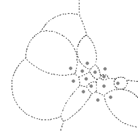
The MW-Voronoi of a set of points
-
(ii)
Calculate genetic distance for all pairs of points that share a weighted Voronoi boundary. Table 2 shows there are 34 out of 91 pairs of genetic distances from the sample data that satisfy the criteria and are highlighted in bold. Join the genetic distance values to the corresponding weighted Voronoi boundaries.
-
(iii)
Initiate the weighted barrier from the weighted Voronoi boundary formed by two points with the largest genetic distance. Figure 2 shows that the largest genetic distance of the sample data, 1.813 (Table 2) is formed by points 4 and 8.
Fig. 2 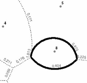
The initialization of WDB from the weighted Voronoi boundary formed by two points (4 and 8) with the largest genetic distance (1.813)
-
(iv)
The weighted barrier is then extended in both directions following the weighted Voronoi boundaries associated with the highest distance. In Fig. 2, 0.972 instead of 0.171, then 0.404 instead of 0.225. The process is continued until it has either formed a closed region around a population, e.g., point 8, or reached the outer limit of the study area. The result is the first level barrier, which bisects the whole space to two regions: the enclosed region surrounds point 8, and the rest of the space.
-
(v)
Depending on the data set, the weighted barrier could be multi-levels. Each upper level barrier bisects the region it belongs to. From each of the bisected regions, the next lower level of weighted barriers are formed following the same criteria as outlined above. Figure 3a shows three levels of WDB barriers formed by the sample data set. For comparison purposes, Fig. 3b shows three levels of MDB barriers formed by the same data set.
Fig. 3 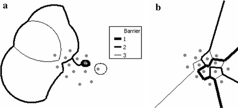
WDB and MDB for the same set of points


3 Testing the WDB method with empirical data
To test the WDB method we use a set of published data of sea scallop collected from 12 locations across coastal areas ranging from Newfoundland, Canada, to New Jersey, USA (Kenchington et al. 2006). At each location, geographic and genetic data are compiled based on measures from six microsatellite loci. This empirical data set includes the geographic longitude and latitude of the locations, pairwise genetic differentiation and the gene diversity (heterozygosity) (Table 1 in p. 1784, Table 3 in p. 1787, and Appendix in p. 1796, Kenchington et al. 2006). The adopted data is summarized in Table 3.
We construct weighted Voronoi polygons for 12 locations using average heterozygosity as weight. As discussed earlier, the use of heterozygosity is only an example to explore the vast potential of incorporating more considerations in constructing weighted instead of ordinary Voronoi polygons. Although there is no direct genetic distance measure provided by this dataset, we take pairwise genetic differentiation (measured by ϑ values) as an indicator of the genetic distance. This approach is supported by previous research in the field, that genetic distance can be estimated as pairwise F ST distancesFootnote 4 for all alleles (Dupanloup et al. 2002), which is equivalent to G ST among populationsFootnote 5 (Nei 1973) and therefore quite similar to Weir and Cockerham’s θ (1984),Footnote 6 only that θ can be negative values (Culley et al. 2002). According to the WDB method, there are a total of 30 pairs of genetic differentiations need to be considered after the construction of the weighted Voronoi polygons. We link those pairwise differentiation values to every weighted Voronoi boundary and begin the barrier detection process starting from the maximum weighted boundary. In Fig. 4, the first three levels of WDB are captured. For the purpose of comparison, the first three levels of MDB are also constructed using Monmonier’s algorithm. We have the following major findings.

MDB and WDB delineation of the sample data
First, there are more shape variations in the WDB boundaries than in the MDB boundaries. Instead of straight lines only and instead of always bisecting two population locations in the MDB, WDB boundaries can be curved and run between two locations based on genetic information such as heterozygosity. For example, the heterozygosity of Georges (Can), 0.701 is smaller than that of Georges (US), 0.793, so the WDB between them is concaved toward the Canadian site showing a relatively smaller and enclosed region. Such a spatial pattern corresponds to the relationship that population with larger gene diversity tends to have larger patch sizes (Banks et al. 2005; Osakabe et al. 2005).
Second, the first barrier of the MDB isolates the site of Georges (US) from others, and the first barrier of the WDB isolates not only that site, but also the Gaspé in the far north. The spatial formation is caused by possible multi-parts and discontinued areas of a weighted Voronoi polygon as described earlier. The pairwise differentiation between the Gaspé and George (US) is 0.006, and average pairwise differentiation between the Gaspé and all other sites except for Georges (US) is 0.022 (Table 3). Therefore, the scallop’s population from the Gaspé is more similar to those from Georges (US) than to the other ten sites, and the WDB method captures this relationship. This WDB delineation matches one of the observations in Kengchington’s (2006) work that “Georges (US) and the Gaspé are significantly differentiated from each other and all other Populations”.
Third, the hierarchy of barriers changes more rapidly in the WDB method. The east [Nfld(TB), Nfld(SP) and PEI) and west (Digby, Annapolis, Wester, Lurcher, Brownis, and Georges (Can)] clusters are formed at the second level of the WDB barrier, and Georges (Can) and Nfld (TB) are distinguished at the third level of the WDB. In contrast, in the MDB, the east and west clusters are not divided until the third level.
4 Discussion
The WDB method calculates genetic distance for weighted Voronoi neighbors as two points separated by a weighted Voronoi polygon boundary, and MDB calculates genetic distance for Voronoi neighbors as two points separated by a Voronoi polygon boundary. By doing so, both within group genetic information (gene diversity), and between group genetic information (genetic distance) are considered. Usually, the number of weighted Voronoi neighbors is larger than the number of Voronoi neighbors, indicating more relationships are being considered. In our sample data, 34 pairs of genetic distance are calculated for WDB and 31 for MDB.
The spatial pattern of the WDB boundaries are often curved and enclosed, while the MDB boundaries are always straight and often opened (Fig. 3a, b). A MDB boundary between two points is a single-part, and a WDB boundary between two points could be multi-parts and disconnected due to geometric properties of weighted Voronoi diagrams (Mu 2004). For instance, in Fig. 5, the two disconnected solid line segments are potential WDB boundaries between points 5 and 12.

Multi-parts of a WDB boundary
Since the Voronoi and TIN are mathematical duals, MDB always run between points that are connected by TIN edges, thus potentially there is a MDB boundary between them. However, WDB is not constrained by this criterion. In Fig. 6, WDB boundary a is formed by points 4 and 12, and such a boundary is not possible for MDB because there is no TIN edge connecting the two points. In our sample data, there are 42 segments of WDB boundaries, 33 of them are between TIN-connected points, and the rest 9 are between non-TIN-connected points.

WDB boundary formed by non-TIN-connected points
Our WDB method tessellates sample points with a weighted Voronoi diagram. Genetic attribute values of each sample point determines the weight, thus the genetic discontinuities between points will not always be the bisection between them. The WDB boundaries are constructed based on weighted Voronoi and can generate hierarchical levels. Segments of WDB boundaries have more variations than those in MDB. They can be multi-parts and disconnected, and can be characterized beyond the straight lines of the MDB and often scribe circular curves.
5 Summary and conclusion
Identifying barriers of species and characterize their effects on spatial distribution provide essential background information to research in landscape ecology, population genetics, biogeography, historical biogeography, and phylogeography. Overall, WDB provides quick and straightforward improvements to the drawbacks of MDB. WDB integrates more sample location relationships into the barrier construction and reveals potential barriers that would otherwise go undetected. WDB incorporates both within group and between group genetic information, and delineates the barriers as a more complex pattern.
Besides the WDB, there are other techniques being explored for boundary delineation that make use of simulated annealing algorithm (Dupanloup et al. 2002), Bayesian criteria or specific distance-decay behaviors (Guillot et al. 2005; Santos et al. 2008; Culley et al. 2002; Guiller et al. 2006; Hull et al. 2008; Manel et al. 2003; Sambridge 1998). We argue the method introduced here is an alternative approach, and a beginning in initiating and integrating more spatial modeling and methods into the problem solving process. This raises an interesting discussion on whether gene diversity only should be applied to assign weights to each population site. Further research will explore other weighted attributes and test the method on data with genetic distances collected from microsatellite markers. Furthermore, embedded within a GIS environment, we explore the correlation of genetic discontinuities detected based on our weighted method and landscape features.
New spatial algorithms that decompose observations or data points into meaningful objects, presents us with a variety of ideas for delineating barriers. The WDB defines a more appropriate model and logically should map more realistic barriers. These new benchmarks can prove quite useful in characterizing spatial patterns and can lead to more enlightened hypotheses or at the very least, help us ask more intelligent questions. Built upon this additional understanding of geospatial genetic variations, future research should be extended to not only the static forms, but also dynamic processes of landscape genetics.
Notes
The additively weighted Voronoi diagram (AW-Voronoi): d aw(x, p) = d e (x, p) − w(p), and region(p) = {x|d aw(x, p) ≤ d aw(x, q), q in S}.
The compoundly weighted Voronoi diagram (CW-Voronoi): Let w1(p) be the multiplicative weight of point p, and let w2(p) be the additive weight of point p. The compoundly weighted Voronoi diagram is actually a combination of MW-Voronoi and AW-Voronoi, where d cw(x, p) = d e (x, p)/w1(p) − w2(p), and region(p) = {x|d cw(x, p) ≤ d cw(x, q), q in S}.
The power diagram (PW-Voronoi): d pw(x, p) = d 2 e (x, p) − w(p), and region(p) = {x|d pw(x, p) ≤ d pw(x, q), q in S} (Okabe et al. 2000).
F ST is the reduction in diversity (heterozygosity) expected with random mating at one level of population hierarchy relative to another more inclusive level. F ST = (H T − H S )/H T , where H T is the genetic diversity within the total population, and H S is the mean of all subpopulation diversity (Wright 1951).
Weir and Cockerham’s θ is the unbiased estimator of F ST that corrects for error associated with incomplete sampling of a population. \( \hat{\theta} = a/(a + b + c), \) where a = the variance between population, b = the variance between individuals within populations, c = the variance between gametes within individuals (Weir and Cockerham 1984).
References
Aurenhammer F, Edelsbrunner H (1984) An optimal algorithm for constructing the weighted Voronoi diagram in the plane. Pattern Recognit 17(2):251–257. doi:10.1016/0031-3203(84)90064-5
Banks SC, Finlayson GR, Lawson SJ, Lindenmayer DB, Paetkau D, Ward SJ, Taylor AC (2005) The effects of habitat fragmentation due to forestry plantation establishment on the demography and genetic variation of a marsupial carnivore, Antechinus agilis. Biol Conserv 122(4):581–597. doi:10.1016/j.biocon.2004.09.013
Boattini A, Villegas MJB, Pettener D (2007) Genetic structure of La Cabrera, Spain, from surnames and migration matrices. Hum Biol 79(6):649–666
Bowser G (1996) Integrating ecological tools with remotely sensed data: modeling animal dispersal on complex landscapes. In: Paper read at third international conference/workshop on integrating GIS and environmental modeling, 21–26 January, Santa Fe, NM
Culley TM, Wallace LE, Gengler-Nowak KM, Crawford DJ (2002) A comparison of two methods of calculating GST, a genetic measure of population differentiation. Am J Bot 89(3):460–465. doi:10.3732/ajb.89.3.460
Dupanloup I, Schneider S, Excoffier L (2002) A simulated annealing approach to define the genetic structure of populations. Mol Ecol 11(12):2571–2581. doi:10.1046/j.1365-294X.2002.01650.x
Epperson BK (2003) Geographical genetics. Princeton University Press, Princeton
Fearnhead P (2007) On the choice of genetic distance in spatial-genetic studies. Genetics 177(1):427–434. doi:10.1534/genetics.107.072538
Fievet V, Touzet P, Arnaud JF, Cuguen J (2007) Spatial analysis of nuclear and cytoplasmic DNA diversity in wild sea beet (Beta vulgaris ssp. maritima) populations: do marine currents shape the genetic structure? Mol Ecol 16(9):1847–1864. doi:10.1111/j.1365-294X.2006.03208.x
Fukamachi K, Iida S, Nakashizuka T (1996) Landscape patterns and plant species diversity of forest reserves in the Kanto region, Japan. Vegetatio 124(1):107–114. doi:10.1007/BF00045149
Guiller A, Bellido A, Coutelle A, Madec L (2006) Spatial genetic pattern in the land mollusc Helix aspersa inferred from a ‘centre-based clustering’ procedure. Genet Res 88(1):27–44. doi:10.1017/S0016672306008305
Guillot G, Estoup A, Mortier F, Cosson JF (2005) A spatial statistical model for landscape genetics. Genetics 170(3):1261–1280. doi:10.1534/genetics.104.033803
Hamrick JL, Godt MJW (1990) Allozyme diversity in plant species. In: Brown AHD (ed) Plant population genetics, breeding and genetic resources.. Sinauer Associates, Sunderland, pp 43–63
Hedrick PW (2005) A standardized genetic differentiation measure. Evolution Int J Org Evolution 59(8):1633–1638
Hu LJ, Uchiyama K, Shen HL, Saito Y, Tsuda Y, Ide Y (2008) Nuclear DNA microsatellites reveal genetic variation but a lack of phylogeographical structure in an endangered species, Fraxinus mandshurica, across north-east China. Ann Bot (Lond) 102(2):195–205. doi:10.1093/aob/mcn074
Hull JM, Hull AC, Sacks BN, Smith JP, Ernest HB (2008) Landscape characteristics influence morphological and genetic differentiation in a widespread raptor (Buteo jamaicensis). Mol Ecol 17(3):810–824
Kenchington EL, Patwary MU, Zouros E, Bird CJ (2006) Genetic differentiation in relation to marine landscape in a broadcast-spawning bivalve mollusc (Placopecten magellanicus). Mol Ecol 15(7):1781–1796. doi:10.1111/j.1365-294X.2006.02915.x
Leclerc E, Mailhot Y, Mingelbier M, Bernatchez L (2008) The landscape genetics of yellow perch (Perca flavescens) in a large fluvial ecosystem. Mol Ecol 17(7):1702–1717. doi:10.1111/j.1365-294X.2008.03710.x
Manel S, Schwartz MK, Luikart G, Taberlet P (2003) Landscape genetics: combining landscape ecology and population genetics. Trends Ecol Evol 18(4):189. doi:10.1016/S0169-5347(03)00008-9
Manni F, Leonardi P, Barakat A, Rouba H, Heyer E, Klintschar M, McElreavey K, Quintana-Murci L (2002) Y-chromosome analysis in Egypt suggests a genetic regional continuity in northeastern Africa. Hum Biol 74(5):645–658. doi:10.1353/hub.2002.0054
Manni F, Guerard E, Heyer E (2004) Geographic patterns of (genetic, morphologic, linguistic) variation: how barriers can be detected by using Monmonier’s algorithm. Hum Biol 76(2):173–190. doi:10.1353/hub.2004.0034
Michels E, Cottenie K, Neys L, De Gelas K, Coppin P, De Meester L (2001) Geographical and genetic distances among zooplankton populations in a set of interconnected ponds: a plea for using GIS modelling of the effective geographical distance. Mol Ecol 10(8):1929–1938. doi:10.1046/j.1365-294X.2001.01340.x
Mu L (2004) Polygon characterization with the multiplicatively weighted Voronoi diagram. Prof Geogr 56(2):223–239
Nei M (1973) Analysis of gene diversity in subdivided populations. Proc Natl Acad Sci USA 70:3321–3323. doi:10.1073/pnas.70.12.3321
Nei M (1987) Molecular evolutionary genetics. Columbia University Press, New York
Okabe A, Boots B, Sugihara K, Chiu SN (2000) Spatial tessellations, concepts and applications of Voronoi diagrams. Wiley, New York
Osakabe M, Goka K, Toda S, Shintaku T, Amano H (2005) Significance of habitat type for the genetic population structure of Panonychus citri (Acari: Tetranychidae). Exp Appl Acarol 36(1–2):25–40. doi:10.1007/s10493-005-1672-1
Radke JD (1998) Boundary generators for the 21st Century, a proximity based classification method. In: 50th anniversary proceedings. Department of City and Regional Planning, University of California, Berkeley
Ratkiewicz M, Borkowska A (2006) Genetic structure is influenced by environmental barriers: empirical evidence from the common vole Microtus arvalis populations. Acta Theriol (Warsz) 51(4):337–344
Sambridge M (1998) Exploring multidimensional landscapes without a map. Inverse Probl 14(3):427–440. doi:10.1088/0266-5611/14/3/005
Santos C, Abade A, Lima M (2008) Testing hierarchical levels of population sub-structuring: the Azores Islands (Portugal) as a case study. J Biosoc Sci 40(4):607–621. doi:10.1017/S0021932007002477
Slatkin M (1987) Gene flow and the geographic structure of natural-populations. Science 236(4803):787–792. doi:10.1126/science.3576198
Slatkin M (1993) Isolation by distance in equilibrium and nonequilibrium populations. Evolution Int J Org Evolution 47(1):264–279. doi:10.2307/2410134
Tobler WR (1970) Computer movie simulating urban growth in Detroit region. Econ Geogr 46(2):234–240. doi:10.2307/143141
Weir BS (1990) Genetic data analysis: methods for discrete population genetic data. Sinauer Associates, Sunderland
Weir BS, Cockerham CC (1984) Estimating F-statistics for the analysis of population structure. Evolution Int J Org Evolution 38(6):1358–1370. doi:10.2307/2408641
Wright S (1951) The genetical structure of populations. Ann Eugen 15:323–354
Open Access
This article is distributed under the terms of the Creative Commons Attribution Noncommercial License which permits any noncommercial use, distribution, and reproduction in any medium, provided the original author(s) and source are credited.
Author information
Authors and Affiliations
Corresponding author
Rights and permissions
Open Access This is an open access article distributed under the terms of the Creative Commons Attribution Noncommercial License (https://creativecommons.org/licenses/by-nc/2.0), which permits any noncommercial use, distribution, and reproduction in any medium, provided the original author(s) and source are credited.
About this article
Cite this article
Mu, L., Radke, J. A weighted difference barrier method in landscape genetics. J Geogr Syst 11, 141–154 (2009). https://doi.org/10.1007/s10109-009-0079-7
Received:
Accepted:
Published:
Issue Date:
DOI: https://doi.org/10.1007/s10109-009-0079-7