
Abstract
Embedded real-time systems generate state sequences where time elapses between state changes. Ensuring that such systems adhere to a provided specification of admissible or desired behavior is essential. Formal model-based testing is often a suitable cost-effective approach. We introduce an extended version of the formalism of symbolic graphs, which encompasses types as well as attributes, for representing states of dynamic systems. Relying on this extension of symbolic graphs, we present a novel formalism of timed graph transformation systems (TGTSs) that supports the model-based development of dynamic real-time systems at an abstract level where possible state changes and delays are specified by graph transformation rules. We then introduce an extended form of the metric temporal graph logic (MTGL) with increased expressiveness to improve the applicability of MTGL for the specification of timed graph sequences generated by a TGTS. Based on the metric temporal operators of MTGL and its built-in graph binding mechanics, we express properties on the structure and attributes of graphs as well as on the occurrence of graphs over time that are related by their inner structure. We provide formal support for checking whether a single generated timed graph sequence adheres to a provided MTGL specification. Relying on this logical foundation, we develop a testing framework for TGTSs that are specified using MTGL. Lastly, we apply this testing framework to a running example by using our prototypical implementation in the tool AutoGraph.
1 Introduction
Software has become an intrinsic part of parallel embedded real-time systems, which need to realize increasingly advanced functionality with complex coordination behavior. The technical challenges for developing such embedded real-time systems with a high degree of parallelism, data dependencies, and timing constraints that must adhere to a given specification are manifold [25, 26, 37]. Moreover, formal verification of models of such complex systems is often infeasible since (a) fully automatic approaches fall short due to undecidability problems or the state-space explosion problem, whereas (b) manual verification approaches require additional expertise and an excessive amount of resources. Formal model-based testing approaches aim at providing a well-balanced tradeoff between the computational costs and the resulting degree of confidence in a broad spectrum of domains [18, 20, 35, 57].
Graph transformation with its visual notation is well-suited for modeling and developing complex dynamic systems where states can be represented by graphs [29]. For instance, rule-based graph transformation supports the modeling of distribution in decentralized systems, modifications of connectivity as in dynamically established collaborations, computations on values and subgraphs, as well as permits a reconfiguration of systems at runtime with powerful mechanisms for controlling rule applicability [67]. However, the expressiveness of graph transformation systems prevents fully automatic analysis due to undecidability in general. Moreover, the emerging behavior may be highly influenced by complex dependencies between rules of the transformation system, which results in a difficult and error-prone modeling phase.
To improve support for the described setting, we introduce a testing approach for timed graph transformation systems (TGTSs) (see Sect. 9 for a comparison with other TGTS formalisms). Well-established metric temporal logics such as MTL [60] relying on atomic propositions are insufficient for the specification of TGTSs when more complex metric temporal properties are to be expressed. In particular, we aim at expressing properties where graphs occurring at different points in time are to be related by their inner structure. Examples of such properties refer to substructures that are monitored over a period of time or check for the existence of nodes or edges with certain attribute values. To express such properties, we build upon graph logics [43, 78] where bindings for subgraphs is a first-class citizen.
As a technical prerequisite to the modeling and testing of TGTSs, we extend the notion of symbolic graphs [71, 73, 74, 82] by adding so-called global variables. Attribute values used in these symbolic graphs are restricted using attribute conditions of an attribute logic. We then define a basic graph logic BGL that is an adaptation of the logic of (nested) graph conditions on symbolic graphs from [82]. The logic BGL additionally permits quantification over potential attribute values using the introduced global variables as in first-order logic and improves applicability by means of a novel operator for managing context in logical conditions. Once again relying on the notion of global variables, we then obtain a suitable notion of graph transformation for symbolic graphs based on [71, 74], which also extends to the case of TGTSs. Furthermore, we develop a graph logic GL, which extends the basic graph logic BGL with a special operator, which can be employed to concisely state properties by simultaneously managing context and stating conditions on attribute values. Building upon our previous work in [38, 81] where we first introduced the metric temporal graph logic (MTGL), we now employ the two novel metric temporal operators  (called \(delta{\text {-}}{}lock \)) and \(\boxdot \) (called \(delta{\text {-}}{}release \)). Compared to [38, 81], these operators additionally permit to express properties on the steps in the past e.g. involving the since operator known from MTL and handle binding of graph elements and attribute values at a more fundamental level. In more detail, we permit that graph elements that have been matched may be removed in the future and that they have not necessarily existed in the past, that the creation and deletion of graph elements can be specified rather than only their (non)existence, and that attribute values from different graphs are compared. Finally, also for the until and since operators (which are special cases of the delta-lock operator), we introduce the delta-release operator. Using this operator, we additionally permit to check properties also in the reverse direction in the timed graph sequence. For example, when using the until operator, we allow for the case that the condition that is to be invariantly satisfied depends on how the property that is to be satisfied at a specified timepoint in the future is satisfied.

Overview of our approach
A general overview of our approach is visualized in Fig. 1. We develop support for checking the satisfaction of a timed graph sequence obtained from a TGTS w.r.t. a formal specification given in the form of (a set of) conditions from MTGL. To this end, we verify encodings of higher-level operators such as delta-lock and delta-release into lower-level operators for iterated graph pattern matching. On the foundation of these theoretical results, we provide a formal testing approach for TGTSs by employing standard methods for generating diverse timed graph sequences from TGTSs using randomization to resolve nondeterminism. In particular, we provide (a) encodings for translating a condition \(\psi \) from MTGL into a condition \(\phi \) of BGL and (b) a folding operation for translating a finite timed graph sequence \(\pi \) into a single graph G preserving all information. We then verify that \(\pi \) satisfies \(\psi \) if and only if G satisfies \(\phi \), which allows for an efficient check of MTGL satisfaction for finite timed graph sequences by reducing this problem to the satisfaction checking problem. All these steps are supported by our prototypical implementation in the tool AutoGraph.
In order to demonstrate our approach, we make use of a running example. Specifically, we consider a model of a real-time operating system in which tasks are executed to produce results and consider the following metric temporal properties.
Example 1
(Properties for Running Example) We consider three properties in our running example, which are formalized using MTGL in Fig. 28.
-
\(\mathbf {P_{1}}\): Each task that is spawned in a system is eventually completed and thereby removed from the system within at most 10000 time units and produces a unique result with a value of \( ok \) and an id that equals the id of the task.
-
\(\mathbf {P_{2}}\): Each new result is obtained from a task with the same id that was spawned at most 10000 time units before and that was present since then.
-
\(\mathbf {P_{3}}\): Every task in a system runs at least once every 1000 time units until it terminates.
We now summarize our main contributions: (a) the integration of global variables in symbolic graphs as the formalism underlying the subsequent developments, (b) the definition of a suitable notion of (timed) graph transformation for symbolic graphs with adequate descriptive expressiveness, (c) the extensions of existing graph logics by introducing restriction and delta-based operators for improving the applicability by allowing to discard parts of matches using contexts, (d) the extension/adaptation of MTGL from [38, 81] described above that permits to express more complex metric temporal properties, and (e) the prototypical implementation of all notions and constructions relevant to our formal testing approach in the tool AutoGraph.
In the future, we envision to improve upon the following aspects of the introduced approach: (a) its effectiveness, by considering suitable additional operators, (b) its efficiency, by applying incremental pattern matching techniques for the generation of timed graph sequences from the TGTS at hand as well as for checking the satisfaction of conditions of MTGL, and (c) its applicability, by developing new means for presenting violations and for filtering definite and potential violations.
The remainder of this paper is organized as follows. In Sect. 2, we introduce the attribute logic AL (which relies on algebraic specifications as explained in more detail in “Appendix A”) which corresponds to attribute logics’ implementations in SMT solvers. Based on this attribute logic AL, we present our extension of symbolic graphs with global variables in Sect. 3 where attribute conditions are used to restrict attribute values occurring in the symbolic graphs. In Sect. 4, we present the basic graph logic BGL with a novel restriction operator. BGL conditions are then used as application conditions of (timed) graph transformation systems introduced in Sect. 5 where we also define the generation of (timed) graph sequences. As an intermediate step, we extend the graph logic BGL resulting in the graph logic GL by integrating a novel delta-based operator, which allows to preserve attribute values across the restriction and extension of matches, in Sect. 6. We then present MTGL in Sect. 7 with the novel metric temporal operators delta-lock and delta-release. The application to the formal testing scenario and details of our prototypical implementation in the tool AutoGraph are discussed in Sect. 8. Finally, Sect. 9 discusses related work and Sect. 10 concludes the paper with a summary and remarks on future work.
Also note the glossary on page 73 covering most symbols introduced throughout the paper.
2 Attribute logic AL
We provide an informal introduction of the attribute logic AL, which is used in the remainder of this paper to specify attribute values in symbolic graphs. In this section, we present the most relevant notations and refer to “Appendix A” for a detailed presentation. The logic AL is the finitary first-order many-sorted logic with equality as supported by standard SMT solvers such as Z3 [68]. Such solvers are shipped with support for sorts such as \(\mathsf {bool}\), \(\mathsf {int}\), \(\mathsf {real}\), and \(\mathsf {string}\) and standard operations on these sorts. For the remainder of this paper, we assume that the attribute conditions (ACs) of AL that are used can be handled by such SMT solvers. In particular, in our prototypical implementation discussed later on in Sect. 8, we rely on Z3 to simplify ACs, check satisfaction of ACs, and check satisfiability of ACs. As checking satisfiability is undecidable for AL, our implementation is ready to report ACs to the user for which Z3 is unable to return a result.
The set of all ACs containing free variables from a set \(X\subseteq \mathcal {X} \) is denoted \(\mathcal {S}^{{\textsf {AC} }} _{X} \) based on a universe \(\mathcal {X} \) of all variables. For example, the AC \(\gamma =\exists \{x\}.\;x\le y+2 \) is an AC over the variable set \(\{y\}\) because y is the only free variable of \(\gamma \). We denote the union of all supported datatypes containing all values by \(\mathcal {V} \). The satisfaction of an AC \(\gamma \) by a variable valuation  is denoted \(\alpha \models _{\mathsf {AC}} \gamma \). Also, if there is such a variable valuation, \(\gamma \) is satisfiable denoted by \({\textsf {sat} }_{\exists } (\gamma ) \). Moreover, if \(\gamma \) is satisfied by each variable valuation, \(\gamma \) is tautological denoted by \({\textsf {sat} }_{\forall } (\gamma ) \). For example, the AC \(\gamma \) from above is tautological because, for each choice of a value for y (given by a variable valuation \(\alpha \)), there is a suitable choice of a value for x as well. Hence, \(\gamma \) can be simplified to the AC \(\top \).
3 Symbolic graphs
(Typed) symbolic graphs have been introduced in [71, 73, 74] in the context of graph transformation on these graphs. Symbolic graphs contain two sets of nodes and edges as usual for graphs but also two further sets of node attributes and edge attributes as in E-Graphs [29] where each node attribute and each edge attribute is connected to a node and an edge, respectively. In E-Graphs, these node attributes and edge attributes are connected to values. In symbolic graphs, node attributes and edge attributes are connected to variables and an AC is used to restrict the possible values for these variables. Note that node and edge attributes have a unique value in attributed graphs based on E-Graphs leading to a unique valuation for node and edge attributes but an AC of a symbolic graph can be satisfied by zero, one, or more different variable valuations.
We adapt the notion of symbolic graphs from [71, 74, 82] as follows. Firstly, we use a single finite AC (see Definition 54 for a formal introduction of ACs) for each symbolic graph instead of a possibly infinite set of ACsFootnote 1 to ensure that the AC of a pullback object can always be constructed.Footnote 2 Secondly, we denote in the following those graph variables as local variables that may be connected to node and edge attributes. Furthermore, we include additional graph variables, called global variables, into a symbolic graph that are disjoint to the local variables. As indicated in Sect. 1 already, these global variables play an important role for our notion of graph transformation for symbolic graphs in Sect. 5 and MTGL in Sect. 7. Global variables are mapped by graph morphisms not necessarily to global variables of the target graph of the morphism. They may also be instantiated to a single value as in a variable valuation.

The plain symbolic graph G with the global variable \(x_4\) and local variables \(x_1\), \(x_2\), \(x_3\) (top left), the symbolic type graph \( TG \) (top right), the typing morphism  (dashed arrows), and the use of the simplified notation (bottom) for G, \( TG \), and \(\tau \). Note that the sorts of variables are only depicted in our simplified notation. The ACs \({G}{.}{{\textsf {ac} }} \) and \({ TG }{.}{{\textsf {ac} }} \) are depicted separately from the graph structure at the bottom in each case. The AC \({G}{.}{{\textsf {ac} }} \) can be satisfied by three different variable valuations. We often use the AC \(\bot \) in symbolic type graphs to ensure that the AC implication in Definition 2 is never violated

Plain symbolic graphs \(G_1\) and \(G_2\) (solid arrows) and the plain symbolic graph morphism  with its components (dashed arrows)
Incorporating global graph variables, we first introduce the notion of plain symbolic graphs for the untyped case.Footnote 3 See Fig. 2 (top left) for an example of a plain symbolic graph G.
Definition 1
(Plain Symbolic Graphs) A tuple \(G=({G}{.}{{\textsf {N} }}, {G}{.}{{\textsf {E} }}, {G}{.}{{\textsf {NA} }}, {G}{.}{{\textsf {EA} }}, {G}{.}{{\textsf {XL} }}, {G}{.}{{\textsf {XG} }}, {G}{.}{{\textsf {Var} }}, {G}{.}{{\textsf {ac} }}, {G{.}{\textsf {s} }_{\textsf {E} }}, {G{.}{\textsf {t} }_{\textsf {E} }}, {G{.}{\textsf {s} }_{\textsf {NA} }}, {G{.}{\textsf {t} }_{\textsf {NA} }}, {G{.}{\textsf {s} }_{\textsf {EA} }}, {G{.}{\textsf {t} }_{\textsf {EA} }})\) is a plain symbolic graph (see Fig. 3 for a visualization), if the sets
-
\({G}{.}{{\textsf {N} }}\) of nodes,
-
\({G}{.}{{\textsf {E} }}\) of edges,
-
\({G}{.}{{\textsf {NA} }}\) of node attributes,
-
\({G}{.}{{\textsf {EA} }}\) of edge attributes,
-
\({G}{.}{{\textsf {XL} }} \subseteq \mathcal {X} \) of local variables, and
-
\({G}{.}{{\textsf {XG} }} \subseteq \mathcal {X} \) of global variables,
are pairwise disjoint,
-
\({G}{.}{{\textsf {Var} }} =({G}{.}{{\textsf {XL} }} \cup {G}{.}{{\textsf {XG} }},{\textsf {type} }_{})\) contains the local and global variables where the function \({\textsf {type} }_{} \) assigns a sort to each variable,Footnote 4
-
\({G}{.}{{\textsf {ac} }} \in \mathcal {S}^{{\textsf {AC} }} _{{G}{.}{{\textsf {XL} }} \cup {G}{.}{{\textsf {XG} }}} \) is an AC defined over the local and global variables, and
-
 ,
, -
 ,
, -
 ,
, -
 ,
, -
 , and
, and -

 ,
, ,
, ,
, ,
, , and
, and
are source and the target functions for edges, node attributes, and edge attributes.
Moreover, we define the following abbreviations.
-
\({G}{.}{{\textsf {X} }} ={G}{.}{{\textsf {XL} }} \cup {G}{.}{{\textsf {XG} }} \) is the set of local and global variables of a plain symbolic graph.
-
\({G}{.}{{\textsf {X} }}{\mathcal {V}} ={G}{.}{{\textsf {X} }} \cup \mathcal {V} \) is the set of local variables, global variables, and values of a plain symbolic graph.
Morphisms between plain symbolic graphs are given by maps between the corresponding sets of elements except for the global variables, which are mapped to the union of global variables and values of the target graph. Intuitively, plain symbolic graph morphisms may restrict/refine the ACs from the source graph to the target graph. This means that plain symbolic graph morphisms must not permit additional variable valuations satisfying the ACs, i.e., each variable valuation that satisfies the AC of the target graph must also satisfy the AC of the source graph where its variables are substituted according to the morphism. This is formally stated as \({\textsf {sat} }_{\forall } ({G_2}{.}{{\textsf {ac} }} \rightarrow {f}{.}{{\textsf {X} }} ({G_1}{.}{{\textsf {ac} }})) \) in the definition below. For example, a morphism  where \({G_1}{.}{{\textsf {ac} }} =(x\ge 2)\) and \({G_2}{.}{{\textsf {ac} }} =(\bar{x}= 4)\) may map x to \(\bar{x}\) using the mapping \({f}{.}{{\textsf {X} }} \). A visualization of the required compatibility with the source and target functions for edges, node attributes, and edge attributes is given in Fig. 3.
Definition 2
(Plain Symbolic Graph Morphisms) A tuple \(f=({f}{.}{{\textsf {N} }}, {f}{.}{{\textsf {E} }}, {f}{.}{{\textsf {NA} }}, {f}{.}{{\textsf {EA} }}, {f}{.}{{\textsf {XL} }}, {f}{.}{{\textsf {XG} }})\) is a plain symbolic graph morphism from graph \(G_1\) to graph \(G_2\), written  , if \(G_1\) and \(G_2\) are plain symbolic graphs,
-
 ,
, -
 ,
, -
 ,
, -
 ,
, -
 , and
, and -

 ,
, ,
, ,
, ,
, , and
, and
are maps between graph components such that compatibility with source and target functions holds, i.e.,
-
\({f}{.}{{\textsf {N} }} \circ {G_1{.}{\textsf {s} }_{\textsf {E} }}={G_2{.}{\textsf {s} }_{\textsf {E} }}\circ {f}{.}{{\textsf {E} }} \),
-
\({f}{.}{{\textsf {N} }} \circ {G_1{.}{\textsf {t} }_{\textsf {E} }}={G_2{.}{\textsf {t} }_{\textsf {E} }}\circ {f}{.}{{\textsf {E} }} \),
-
\({f}{.}{{\textsf {N} }} \circ {G_1{.}{\textsf {s} }_{\textsf {NA} }}={G_2{.}{\textsf {s} }_{\textsf {NA} }}\circ {f}{.}{{\textsf {NA} }} \),
-
\({f}{.}{{\textsf {XL} }} \circ {G_1{.}{\textsf {t} }_{\textsf {NA} }}={G_2{.}{\textsf {t} }_{\textsf {NA} }}\circ {f}{.}{{\textsf {NA} }} \),
-
\({f}{.}{{\textsf {E} }} \circ {G_1{.}{\textsf {s} }_{\textsf {EA} }}={G_2{.}{\textsf {s} }_{\textsf {EA} }}\circ {f}{.}{{\textsf {EA} }} \), and
-
\({f}{.}{{\textsf {XL} }} \circ {G_1{.}{\textsf {t} }_{\textsf {EA} }}={G_2{.}{\textsf {t} }_{\textsf {EA} }} \circ {f}{.}{{\textsf {EA} }} \),
and it holds that
-
\({f}{.}{{\textsf {XL} }} \) and \({f}{.}{{\textsf {XG} }} \) respect the sorts of the variablesFootnote 5 and
-
\(G_2\) has a more restrictive AC compared to \(G_1\), i.e., \({\textsf {sat} }_{\forall } ( {G_2}{.}{{\textsf {ac} }} \rightarrow {f}{.}{{\textsf {X} }} ({G_1}{.}{{\textsf {ac} }}) ) \).
Moreover, we define the following abbreviations.
-
Map of local and global variablesFootnote 6:
 with \({f}{.}{{\textsf {X} }} ={f}{.}{{\textsf {XL} }} \cup {f}{.}{{\textsf {XG} }} \)
 -
Map of local and global variables extended by identity map on values:

with \({f}{.}{{\textsf {X} }}_{\mathcal {V}} ={f}{.}{{\textsf {XL} }} \cup {f}{.}{{\textsf {XG} }} \cup {\textsf {id} } (\mathcal {V}) \)
-
Map of global variables that are mapped to values:
 where A is some subset of \({G_1}{.}{{\textsf {XG} }} \)
with \({f}{.}{{\textsf {X} }}_{\textsf {GM} } ={f}{.}{{\textsf {XG} }} \cap ({G_1}{.}{{\textsf {XG} }} \times \mathcal {V})\)
-
Map of local variables and of global variables when no global variables are mapped to values:
If \({f}{.}{{\textsf {X} }}_{\textsf {GM} } =\varnothing \), then

with \({f}{.}{{\textsf {X} }}_{\textsf {P} } ={f}{.}{{\textsf {X} }} \cap ({G_1}{.}{{\textsf {X} }} \times {G_2}{.}{{\textsf {X} }})\)
 with
with 
 where A is some subset of
The binary composition of two plain symbolic graph morphisms is defined as usual for all components except for the global variables. For global variables we extend the second map \({f_2}{.}{{\textsf {XG} }} \) by the identity function on values that then preserves the values that are generated by the first map \({f_1}{.}{{\textsf {XG} }} \).
Definition 3
(Binary Composition of Plain Symbolic Graph Morphisms) If  and
and  are plain symbolic graph morphisms, then
  with \(f_3=({f_3}{.}{{\textsf {N} }}, {f_3}{.}{{\textsf {E} }}, {f_3}{.}{{\textsf {NA} }}, {f_3}{.}{{\textsf {EA} }}, {f_3}{.}{{\textsf {XL} }}, {f_3}{.}{{\textsf {XG} }})\) where
-
\({f_3}{.}{{\textsf {N} }} ={f_2}{.}{{\textsf {N} }} \circ {f_1}{.}{{\textsf {N} }} \),
-
\({f_3}{.}{{\textsf {E} }} ={f_2}{.}{{\textsf {E} }} \circ {f_1}{.}{{\textsf {E} }} \),
-
\({f_3}{.}{{\textsf {NA} }} ={f_2}{.}{{\textsf {NA} }} \circ {f_1}{.}{{\textsf {NA} }} \),
-
\({f_3}{.}{{\textsf {EA} }} ={f_2}{.}{{\textsf {EA} }} \circ {f_1}{.}{{\textsf {EA} }} \),
-
\({f_3}{.}{{\textsf {XL} }} ={f_2}{.}{{\textsf {XL} }} \circ {f_1}{.}{{\textsf {XL} }} \), and
-
\({f_3}{.}{{\textsf {XG} }} =({f_2}{.}{{\textsf {XG} }} \cup {\textsf {id} } (\mathcal {V}))\circ {f_1}{.}{{\textsf {XG} }} \)
is the composition of plain symbolic graph morphisms \(f_2\) and \(f_1\), written \(f_3=f_2\circ _{{\textsf {p} }}f_1\).
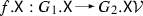
The typing of plain symbolic graphs is formalized using an additional plain symbolic graph morphism \(\tau \) that has a plain symbolic graph G as a source, a symbolic type graph \( TG \) as a target, and does not map any global variables of G to values (see Fig. 2 for an example of a typed symbolic graph, a symbolic type graph, a typing morphism, and the simplified notation for typed symbolic graphs that we use in the remainder of this paper).
Definition 4
(Typed Symbolic Graphs) If G and \( TG \) are plain symbolic graphs,  is a plain symbolic graph morphism, and \(\tau \) does not map any global variables of G to values (i.e., \({\tau }{.}{{\textsf {X} }}_{\textsf {GM} } =\varnothing \)), then \((G,\tau )\) is a typed symbolic graph over a symbolic type graph \( TG \), written \((G,\tau )\in \mathbf {Graphs}_{ TG } \) or simply \((G,\tau )\in \mathbf {Graphs} \) when the type graph is clear from the context.
Morphisms between typed symbolic graphs are then assumed to preserve the typing for all graph elements except for global variables that are mapped to values (recall that the plain symbolic graph morphism ensures already that global variables cannot be matched to values of a different sort).
Definition 5
(Typed Symbolic Graph Morphisms) If  and
and  are two typed symbolic graphs,
  is a plain symbolic graph morphism, and f is compatible with the typing morphisms \(\tau _1\) and \(\tau _2\):
-
\({\tau _1}{.}{{\textsf {N} }} ={\tau _2}{.}{{\textsf {N} }} \circ {f}{.}{{\textsf {N} }} \),
-
\({\tau _1}{.}{{\textsf {E} }} ={\tau _2}{.}{{\textsf {E} }} \circ {f}{.}{{\textsf {E} }} \),
-
\({\tau _1}{.}{{\textsf {NA} }} ={\tau _2}{.}{{\textsf {NA} }} \circ {f}{.}{{\textsf {NA} }} \),
-
\({\tau _1}{.}{{\textsf {EA} }} ={\tau _2}{.}{{\textsf {EA} }} \circ {f}{.}{{\textsf {EA} }} \),
-
\({\tau _1}{.}{{\textsf {XL} }} ={\tau _2}{.}{{\textsf {XL} }} \circ {f}{.}{{\textsf {XL} }} \), and
-
for every \(x\in {G_1}{.}{{\textsf {XG} }} \) and \(y\in {G_2}{.}{{\textsf {XG} }} \) s.t. \({f}{.}{{\textsf {XG} }} (x)=y\) it holds that \({\tau _1}{.}{{\textsf {XG} }} (x)={\tau _2}{.}{{\textsf {XG} }} (y)\),
then f is a typed symbolic graph morphism from \((G_1,\tau _1)\) to \((G_2,\tau _2)\), written  .
.
We define the binary composition of typed symbolic graph morphisms along the lines of the binary composition of plain symbolic graph morphisms.
Definition 6
(Binary Composition of Typed Symbolic Graph Morphisms) If  ,
,  , and
, and  are typed symbolic graph morphisms, and \(f_3=f_2\circ _{{\textsf {p} }}f_1\) is the composition of plain symbolic graph morphisms \(f_2\) and \(f_1\), then \(f_3\) is the composition of typed symbolic graph morphisms \(f_2\) and \(f_1\), written \(f_3=f_2\circ f_1\).
To ease presentation, we handle typing of symbolic graphs and symbolic graph morphisms implicitly, assume a fixed type graph, focus on symbolic graphs that are finite (i.e., symbolic graphs with a finite AC and finite sets of nodes, edges, node attributes, edge attributes, local variables, and global variables) unless stated otherwise, and refer in the following to typed symbolic graphs as symbolic graphs or simply graphs and to typed symbolic graph morphisms as morphisms. See also “Appendix C” for additional definitions and results.
We define two special kinds of morphisms. An inclusion morphism  has only inclusions as components (see Definition 61). An identity morphism
  has only identities as components (see Definition 62).
We state in the following theorem that graphs and morphisms, as introduced here, together with composition and identity morphisms determine a category.
Theorem 1
(Category \(\mathbf {SymbGraphs} \)) If \( Ob \) is the class of graphs from Definition 4, \( Mor (A,B)\) is the set of morphisms of type  from Definition 5, \(\circ \) is the binary composition of morphisms from Definition 6, and \({\textsf {id} } (A) \) is the unique identity morphism, then \(\mathbf {SymbGraphs} =( Ob , Mor ,\circ ,{\textsf {id} })\) is a category.
See page 58 for the proof of this theorem.
As the next step, we discuss several further notions and constructions for the category \(\mathbf {SymbGraphs} \).
The unique empty graph is denoted by \(\varvec{\varnothing } \), contains no graph elements, and has the trivial AC \({\varvec{\varnothing }}{.}{{\textsf {ac} }} =\top \). The empty graph \(\varvec{\varnothing } \) is initial in \(\mathbf {SymbGraphs}\) (see Lemma 3) but other graphs with no graph elements and a tautological AC are initial as well (see Lemma 2) as they are isomorphic to \(\varvec{\varnothing } \). We denote the unique initial morphism of type  by \({\textsf {i} } (G) \).
Partially injective morphisms are used as match morphisms later (see also [33, Definition 7.3, p. 173] where almost injective morphisms have been introduced to be able to map variables noninjectively to values in an otherwise injective match). These morphisms have only injective components except for the component of global variables where they are permitted to map distinct global variables to the same value.
Definition 7
(Partially Injective Morphisms) If  is a morphism with \(f=({f}{.}{{\textsf {N} }},{f}{.}{{\textsf {E} }},{f}{.}{{\textsf {NA} }},{f}{.}{{\textsf {EA} }},{f}{.}{{\textsf {XL} }},{f}{.}{{\textsf {XG} }})\), \({f}{.}{{\textsf {N} }} \), \({f}{.}{{\textsf {E} }} \), \({f}{.}{{\textsf {NA} }} \), \({f}{.}{{\textsf {EA} }} \), and \({f}{.}{{\textsf {XL} }} \) are injective, and for all \(x\in {A}{.}{{\textsf {XG} }} \) and \(y\in {A}{.}{{\textsf {XG} }} \) it holds that \({f}{.}{{\textsf {XG} }} (x)={f}{.}{{\textsf {XG} }} (y)\notin \mathcal {V} \) implies \(x=y\), then f is a partially injective morphism, written
  or \(f\in \mathcal {P} \).
A monomorphism  in \(\mathbf {SymbGraphs}\) (also denoted by \({\textsf {mono} }(f)\) or \(f\in \mathcal {M} \)) is injective on all components and maps no global variables to a value (see Lemma 4). Obviously, every monomorphism is a partially injective morphism as well but not vice versa. An epimorphism
  in \(\mathbf {SymbGraphs}\) (also denoted by \({\textsf {epi} }(f)\) or \(f\in \mathcal {E} \)) is surjective on all components except for the global variables where \({f}{.}{{\textsf {XG} }} \) must map to all global variables of the target graph (see Lemma 5). An isomorphism
  of \(\mathbf {SymbGraphs}\) (also denoted by \({\textsf {isom} }(f)\)) is a monomorphism, an epimorphism, and source and target graphs must have equivalent ACs w.r.t. the mapping of their variables (see Lemma 6).
A cospanFootnote 7 is jointly epimorphic in \(\mathbf {SymbGraphs}\) (denoted by \((f_1,f_2)\in \mathcal {E}' \)) when each graph element (i.e., excluding the set of values \(\mathcal {V} \)) of K is mapped to by \(f_1\) or \(f_2\) (see Lemma 7).
The further categorical notions and constructions in \(\mathbf {SymbGraphs}\) of coproducts describing the disjoint union of two graphs (see Lemma 13), pushouts describing the union of two graphs (see Lemma 9), pullbacks describing the intersection of two graphs (see Lemma 12), \(\mathcal {E} \text {-}\mathcal {P} \) -factorizations describing a decomposition of morphisms (see Lemma 8), and \(\mathcal {E}' \text {-}\mathcal {P} \) -pair-factorizations describing a decomposition of a cospan (see Lemma 15) are covered in “Appendix C”.
An AC inclusion morphism has only identities as components and has a source graph with the trivial AC \(\top \). Hence, every graph G induces an AC inclusion morphism of type  by obtaining \(\bar{G}\) from G by setting the AC of G to \(\top \).
Definition 8
(AC Inclusion Morphisms) If  is a morphism with \(f{=}({f}{.}{{\textsf {N} }},{f}{.}{{\textsf {E} }},{f}{.}{{\textsf {NA} }},{f}{.}{{\textsf {EA} }},\) \({f}{.}{{\textsf {XL} }}, {f}{.}{{\textsf {XG} }})\), \({f}{.}{{\textsf {N} }} \), \({f}{.}{{\textsf {E} }} \), \({f}{.}{{\textsf {NA} }} \), \({f}{.}{{\textsf {EA} }} \), \({f}{.}{{\textsf {XL} }} \), and \({f}{.}{{\textsf {XG} }} \) are identities, and \({\bar{G}}{.}{{\textsf {ac} }} =\top \), then f is the AC inclusion morphism for G, written \(f={\textsf {acInc} } (G) \).
Graphs in which each variable is restricted by an AC to a unique value are called grounded graphs and correspond straightforwardly to E-Graphs.
Definition 9
(Grounded Graphs) If \(G\in \mathbf {Graphs} \) is a graph and a unique variable valuation satisfies \({G}{.}{{\textsf {ac} }} \) (i.e.,  ), then G is a grounded graph, written \({\textsf {grounded} } (G) \).
In fact, each graph G induces a class of such grounded graphs \(G'\), which are obtained by a possible renaming of the graph elements and by restricting the AC of G such that the AC of \(G'\) is satisfied by a unique variable valuation. The renaming of the graph elements is given by a partially injective morphism  that is an epimorphism (to ensure that e.g. no additional vertices are added) but no isomorphism in general.
Definition 10
(Induced Grounded Graphs) If \(G\in \mathbf {Graphs} \) is a graph, then  is the class of all grounded graphs induced by G.
The notion of induced grounded graphs determines the semantics of a graph. Hence, graphs that induce an empty set of grounded graphs (i.e., graphs with an unsatisfiable AC) should be avoided and can be understood to be faulty.
Later in Sects. 4 and 6, we make use of the following operation \({\textsf {overlap} }\), which we adapt from [43] to symbolic graphs with global variables. The operation \({\textsf {overlap} }\) (see Fig. 4) computes a set of pairs of jointly epimorphic monomorphisms that are generated from a given spanFootnote 8 (f, m) of two monomorphisms. Each cospan \((m',f')\) in the returned set ensures that the square consisting of f, m, \(m'\), and \(f'\) commutes and that the common target graph K of \(m'\) and \(f'\) is minimal in the sense that all its elements are mapped to by either \(m'\) or \(f'\). Moreover, we require that the AC of K must be constructed in a way that restricts the variables in K only in the least way possible to be compatible with the two given morphisms f and m.Footnote 9 Note that one of the constructed cospans is the pushout of (f, m): the graph K constructed in that case is minimal due to the universal property of a pushout stating that the pushout object K can be compatibly matched (possibly noninjectively) into every other overlapping graph \(\bar{K}\) as constructed by the operation \({\textsf {overlap} }\). Note that for later applications, we define the result of the operation \({\textsf {overlap} }\) to be a finite set S of cospans by characterizing first all suitable cospans \(S'\) and by then obtaining S as a finite representation of \(S'\) up to isomorphism. Note that in actual implementations, computing S and obtaining \(S'\) from S go hand in hand.
Definition 11
(Operation \({\textsf {overlap} }\) ) If
-
A, B, and C are graphs,
-
 and
and  are monomorphisms,
 -
 are jointly epimorphic monomorphisms,
 -
\(m'\circ f=f'\circ m\), and
-
\({\textsf {sat} }_{\forall } ( {K}{.}{{\textsf {ac} }} \leftrightarrow ( {m'}{.}{{\textsf {X} }} ({B}{.}{{\textsf {ac} }}) \wedge {f'}{.}{{\textsf {X} }} ({C}{.}{{\textsf {ac} }}) ) ) \),
 and
and  are monomorphisms,
 are jointly epimorphic monomorphisms,
then \((m',f')\in S'\) where \(S'\) is a set of cospans.
Moreover, if S is a uniquely defined representation of \(S'\) up to isomorphism,Footnote 10 then \({\textsf {overlap} } (f,m) =S\).

Visualization for the operation \({\textsf {overlap} }\)
4 Basic graph logic
Graph logics are used to specify different kinds of graphs in terms of their graph elements (for symbolic graphs these are nodes, edges, and their attributes). In the past, graph conditions (for labeled graphs) with attribute conditions but without nesting were introduced in [72] and were extended with operators from propositional logic in [70]. Moreover, graph conditions without attribute conditions but with nesting were introduced in [43] for various categories such as labeled graphs (based on a general definition of a weak adhesive HLR category \((C,\mathcal {M})\) with an \(\mathcal {M}\)-initial object). An integration of these two approaches that supports nesting as well as attribute conditions using symbolic graphs was presented in [82].
We now continue this line of research by extending the graph logic presented in [82] to obtain the basic graph logic BGL, which supports symbolic graphs, with the novel integration of global variables and a restriction operator. Note that BGL uses the first-order logic expressive logic AL for specifying attribute values. Moreover, when the type graph does not contain variables, BGL subsumes the logic of nested graph conditions from [43], which is as expressive as first-order logic on graphs [23] as shown in [43, 78]. However, we believe that BGL has an increased expressiveness compared to the logic from [82] since the integration of global variables can be understood as a lifting of the existential quantification of ACs to the graph level, which is unavailable for the first-order logic on graphs.Footnote 11 Also, the integration of the restriction operator enhances applicability of the logic by increasing its descriptive expressiveness.
4.1 Graph conditions and satisfaction relation
The basic graph conditions (BGCs) of BGL feature the two propositional connectives \(\wedge \) (called \(conjunction \)) and \(\lnot \) (called \(negation \)) as well as the additional operators \(\exists \) (called \(exists \)) and \(\nu \) (called \(restrict \)) for extending and restricting matches into a symbolic graph (called host graph), respectively.
The \(exists \) operator requires an extension of a given match into the host graph by matching further graph elements (such as nodes and edges) or by describing attribute values of already matched variables more precisely. Hence, the \(exists \) operator extends a context that is given by the match.
The novel \(restrict \) operator allows to select a submatch of a given match, which matches fewer elements but matches these elements in the same way as the given match. Hence, the \(restrict \) operator shrinks a context that is given by the match.
The operators of BGL can be combined freely in BGCs with the requirement that \(exists \) and \(restrict \) operators must build upon the symbolic graph that represents the given context as usual. Technically, the operator \(exists \) describes the extension of a finite context graph H to a finite context graph \(H'\) via a monomorphism  and the \(restrict \) operator describes the restriction of a finite context graph H to a finite context graph \(H'\) via a monomorphism
  .
.
Definition 12
(Basic Graph Conditions (BGCs)) If \(H\in \mathbf {Graphs} \) is a graph, then \(\bar{\phi }\in \mathcal {S}^{\mathsf {BGC}} _{H} \) is a basic graph condition (BGC) over H, if one of the following items applies.
-
\(\bar{\phi }=\wedge S \) and \(S\mathrel {\subseteq _{\mathsf {fin}}} \mathcal {S}^{\mathsf {BGC}} _{H} \).
-
\(\bar{\phi }=\lnot \phi \) and \(\phi \in \mathcal {S}^{\mathsf {BGC}} _{H} \).
-
 and \(\phi \in \mathcal {S}^{\mathsf {BGC}} _{H'} \).
 -
 and \(\phi \in \mathcal {S}^{\mathsf {BGC}} _{H'} \).
 and
and  and
and Moreover, we define the following abbreviations.
-
true: \(\top =\wedge \varnothing \)
-
false: \(\bot =\lnot \top \)
-
disjunction: \(\vee S =\lnot (\wedge \{\lnot \phi \mid \phi \in S\}) \)
-
universal quantification: \(\forall (f,\phi ) =\lnot \exists (f,\lnot \phi ) \)

An example for BGC satisfaction with nesting and negation. a The BGC \(\phi \), which formalizes the property “Each node \(a{\text {:A}}\) has an edge \(e_1{\text {:eAB}}\) to a node \(b{\text {:B}}\) without self-loop \(e_2{\text {:eBB}}\).” b The host graph G, which satisfies \(\phi \) from a because every of two possible extensions of the empty match \({\textsf {i} } (G) \) (\(m_1=\{a\mapsto a_0\}\) and \(m_2=\{a\mapsto a_1\}\)) can be further extended to matches (\(m_1'=\{a\mapsto a_0,e_1\mapsto e_1,b\mapsto b_0\}\) and \(m_2'=\{a\mapsto a_1,e_1\mapsto e_2,b\mapsto b_0\}\)). Moreover, each of these two matches \(m_1'\) and \(m_2'\) then cannot be extended to also match a self-loop on \(b_0\)

An example for BGC satisfaction with global variables and ACs. a The BGC \(\phi \) stating “There is a node \(a{\text {:A}}\) connected via some \(e{\text {:eAB}}\) to a node \(b{\text {:B}}\) with an \(\text {id} \) attribute of some \(x\in \mathbf {N} \) and for every \(y\in \mathbf {N} \) smaller or equal x, the node a has an edge \(e'{\text {:eAC}}\) to a node \(c{\text {:C}}\) with \(\text {id} \) attribute of y.” b The host graph G, which satisfies \(\phi \) from a because the empty match \({\textsf {i} } (G) \) can be extended to a match (\(m_0=\{a\mapsto a_0,x\mapsto 2\}\)) that can be further extended to a match (\(m_1=\{a\mapsto a_0,x\mapsto 2,e\mapsto e_3,b\mapsto b_0\}\)) where \(b_0\) has an \(\text {id} \) attribute value equal to \(2=m_1(x)\). Moreover, each extension of \(m_0\) that maps y to some integer between 0 and 2 (e.g. \(m_2=\{a\mapsto a_0,x\mapsto 2,e\mapsto e_3,y\mapsto 0\}\)) can be extended to a match (e.g. \(m_3=\{a\mapsto a_0,x\mapsto 2,e\mapsto e_3,y\mapsto 0,e'\mapsto e_0,c\mapsto c_0\}\)) where \(c_0\) has an \(\text {id} \) attribute value equal to 0. Similar extensions can be found when using 1 and 2 as possible values for y

An example for BGC satisfaction with restriction as well as encoding of the restrict operator. a The BGC \(\phi \), which formalizes the property “There is a node \(a{\text {:A}}\) that has an edge \(e{\text {:eAB}}\) to a node \(b{\text {:B}}\) such that when selecting only the node a as a context, the node a has an edge \(e_1{\text {:eAB}}\) to a node \(b{\text {:B}}\) that has a self-loop \(e_2{\text {:eBB}}\).” b The host graph G, which satisfies \(\phi \) from a because the empty match \({\textsf {i} } (G) \) can be extended to a match (\(m=\{a\mapsto a_1,e\mapsto e_0,b\mapsto b_0\}\)) that can be restricted to a match (\(m'=\{a\mapsto a_1\}\)) that can again be extended to a match (\(m''=\{a\mapsto a_1,e\mapsto e_1,b\mapsto b_1,e_2\mapsto e_2\}\)). Note that if the empty match \({\textsf {i} } (G) \) is extended to the match (\(\bar{m}=\{a\mapsto a_0,e\mapsto e_3,b\mapsto b_0\}\)), this match can be restricted to the match (\(\bar{m}'=\{a\mapsto a_0\}\)) but then there is no further suitable extension of this match. c The encoding of \(\phi \) from a without restrict operator
In BGCs in our examples, for improved readability, we only use inclusions  and employ the notation introduced below for their visualization.
Notation 1
(Morphisms in BGCs ) For a BGC  , we visualize f by (a) all graph elements that are in \(H'-H\), (b) all graph elements that are connected to elements in \(H'-H\), (c) the set \(S_2-S_1\) of BGCs, if \({H}{.}{{\textsf {ac} }} =\wedge S_1 \) and \({H'}{.}{{\textsf {ac} }} =\wedge S_2 \), or otherwise the AC \({H'}{.}{{\textsf {ac} }} \), if it is not \(\top \), and (d) the set \({H'}{.}{{\textsf {XG} }}-{H}{.}{{\textsf {XG} }} \) of global variables, if it is not empty.
For a BGC  , we visualize f by (a) all graph elements that are in \(H'\), (b) the AC \({H'}{.}{{\textsf {ac} }} \), if it is not \(\top \), and (c) the set \({H'}{.}{{\textsf {XG} }} \) of global variables, if it is not empty.
See Fig. 5 for an example of a BGC demonstrating the use of nesting and BGL operators not making use of attributes, Fig. 6 for an example of a BGC focusing on the attribute part in combination with the usage of the novel global variables, and Fig. 7 for an example of a BGC making use of the novel restrict operator.
The satisfaction relation for BGL is given below in the form of an inductive definition that relies on the inductive definition of BGCs. The definition follows [43, 82] for the operators \(conjunction \), \(negation \), and \(exists \). However, it also defines the satisfaction for the additional restrict operator and relies on partially injective morphisms that are allowed to map global variables to values. For the case when checking a graph against a BGC, the satisfaction relation is defined using the initial morphism  and BGCs over the empty graph \(\varvec{\varnothing } \). This case depends on the satisfaction relation where a partially injective morphism
  , which represents a match of the current context graph H into the host graph G, is checked against a BGC over the graph H. For conjunction and negation, the satisfaction relation is defined as expected. For satisfaction of the BGC
  , the definition requires an extension of the match m (as in [43, 82]) in the form of a match
  that satisfies the subcondition \(\phi \) and that is consistent with f in the sense of the commutation condition \(m'\circ f=m\). This condition means (if f is an inclusion) that \(m'\) is defined as m for all elements in H and that \(m'\) has additional mappings for the elements that are in \(H'\) but not in H. This commutation condition also guarantees that the global variables in H/\(H'\) that are mapped by m/\(m'\) to values in \(\mathcal {V} \) are evaluated to these values throughout the satisfaction check for the entire subcondition \(\phi \). Finally, the satisfaction relation requires for the BGC
  that the restricted match
  satisfies the subcondition \(\phi \). Note that the satisfaction check for the exists operator may not succeed when there is no suitable extension match \(m'\) but that the restrict operator always succeeds in restricting the given match m to the match \(m\circ f\).
Definition 13
(Satisfaction of BGCs) If \(\bar{\phi }\in \mathcal {S}^{\mathsf {BGC}} _{H} \) is a BGC and  is a partially injective morphism, then \(m\models _{\mathsf {BGC}} \bar{\phi } \), if one of the following items applies.
-
\(\bar{\phi }=\wedge S \) and \(\forall \phi \in S.\;m\models _{\mathsf {BGC}} \phi \).
-
\(\bar{\phi }=\lnot \phi \) and \(m\not \models _{\mathsf {BGC}} \phi \).
-
 and there is
  s.t. \(m=m'\circ f\) and \(m'\models _{\mathsf {BGC}} \phi \).
 -
 and \(m\circ f\models _{\mathsf {BGC}} \phi \).
 and there is
  s.t.
s.t.  and
and Also, if \(\bar{\phi }\in \mathcal {S}^{\mathsf {BGC}} _{\varvec{\varnothing }} \) and \({\textsf {i} } (G) \models _{\mathsf {BGC}} \bar{\phi } \), then \(G\models _{\mathsf {BGC}} \bar{\phi } \).
See Fig. 5, Fig. 6, and Fig. 7 for examples of satisfaction checks for BGCs. Moreover, a discussion on the inherent problems of BGL satisfaction checking and an operationalization of it is given in “Appendix B.”
4.2 Operation \({\textsf {shift} }\) and encoding of restrict
We adapt and extend the operation \({\textsf {shift} }\) from [32, pp. 15-16] and [82, Def. 17, p. 716] to our setting of symbolic graphs with global variables and the additional restrict operator.Footnote 12 Intuitively, the operation \({\textsf {shift} }\) describes the propagation of a BGC over a morphism (which we assume to be a monomorphism here) preserving the semantics w.r.t. the satisfaction relation. The operation is commonly used as in [32] for propagating BGCs that restrict rule applicability in the context of graph transformation.Footnote 13
Definition 14
(Operation \({\textsf {shift} }\) ) If \(\bar{\phi }\in \mathcal {S}^{\mathsf {BGC}} _{H} \), \(\bar{\phi }'\in \mathcal {S}^{\mathsf {BGC}} _{G} \) are BGCs and  is a monomorphism, then \({\textsf {shift} } (m,\bar{\phi }) =\bar{\phi }'\), if one of the following items applies.
-
\(\bar{\phi }=\wedge S \) and \(\bar{\phi }'=\wedge \{{\textsf {shift} } (m,\phi ) \mid \phi \in S\} \).
-
\(\bar{\phi }=\lnot \phi \) and \(\bar{\phi }'=\lnot {\textsf {shift} } (m,\phi ) \).
-
 and
and\(\bar{\phi }'{=}\vee \{\exists (f',{\textsf {shift} } (m',\phi )) \mid (m',f'){\in }{\textsf {overlap} } (f,m) \} \).
-
 and \(\bar{\phi }'=\nu (m\circ f,\phi ) \).
 and
and and
and In the following, we also adapt the standard soundness result for the \({\textsf {shift} }\) operation from [32, pp. 15-17] to our setting (see Fig. 8 for a visualization).
Theorem 2
(Soundness of \({\textsf {shift} }\) ) If  is a monomorphism,
  is a partially injective morphism and \(\phi \in \mathcal {S}^{\mathsf {BGC}} _{H} \) is a BGC, then \(m_2\circ m_1\models _{\mathsf {BGC}} \phi \) iff \(m_2\models _{\mathsf {BGC}} {\textsf {shift} } (m_1,\phi ) \).
See page 68 for the proof of this theorem.

Visualization for the soundness of \({\textsf {shift} }\)
We now provide the operation \({\textsf {enc} }_{\nu }\), which encodes the restrict operator using the other operators of BGL. This operation thereby shows that the novel restrict operator increases the descriptive expressiveness but not the expressiveness of the logic. Also, procedures for satisfaction checking must then not be developed for the entire logic but only for the fragment not using the restrict operator. The encoding relies on the operation \({\textsf {shift} }\) to replace instances of restrict operators. See Fig. 7 for an example of the application of the operation \({\textsf {enc} }_{\nu }\) .
As already motivated for the definition of the \({\textsf {shift} }\) operation above, the two perspectives of shifting a BGC forwards over a monomorphism  and describing the condition BGC in the context restricted by f are symmetric.
Definition 15
(Operation \({\textsf {enc} }_{\nu }\) ) If \(\bar{\phi }\) and \(\bar{\phi }'\) are BGCs from \(\mathcal {S}^{\mathsf {BGC}} _{H} \), then \({\textsf {enc} }_{\nu } (\bar{\phi }) =\bar{\phi }'\), if one of the following items applies.
-
\(\bar{\phi }=\wedge S \) and \(\bar{\phi }'=\wedge \{{\textsf {enc} }_{\nu } (\phi ) \mid \phi \in S\} \).
-
\(\bar{\phi }=\lnot \phi \) and \(\bar{\phi }'=\lnot {\textsf {enc} }_{\nu } (\phi ) \).
-
 and \(\bar{\phi }'=\exists (f,{\textsf {enc} }_{\nu } (\phi )) \).
 -
 and \(\bar{\phi }'={\textsf {shift} } (f,\phi ) \).
 and
and  and
and We now state the correctness of this encoding.
Theorem 3
(Soundness of \({\textsf {enc} }_{\nu }\)) If \(\phi \in \mathcal {S}^{\mathsf {BGC}} _{H} \) is a BGC and  is a partially injective morphism, then \(m\models _{\mathsf {BGC}} \phi \) iff \(m\models _{\mathsf {BGC}} {\textsf {enc} }_{\nu } (\phi ) \).
See page 70 for the proof of this theorem.
The encoding operation \({\textsf {enc} }_{\nu }\) is also sound for graphs as a direct consequence of Theorem 3.
Corollary 1
(Soundness of \({\textsf {enc} }_{\nu }\) for Graphs) If \(\phi \in \mathcal {S}^{\mathsf {BGC}} _{\varvec{\varnothing }} \) is a BGC and \(G\in \mathbf {Graphs} \) is a graph, then \(G\models _{\mathsf {BGC}} \phi \) iff \(G\models _{\mathsf {BGC}} {\textsf {enc} }_{\nu } (\phi ) \).
See page 70 for the proof of this corollary.
Note that the encoding operation \({\textsf {enc} }_{\nu }\) may increase the size of a BGC drastically because the replacement condition is based on the set of graph overlappings computed by \({\textsf {shift} }\) via \({\textsf {overlap} }\) that grows exponentially with its inputs. We conclude that the operator restrict increases the descriptive expressiveness as it allows to state certain properties more concisely. The operation \({\textsf {enc} }_{\nu }\) is supported by our prototypical implementation in AutoGraph.
5 Graph transformation
The foundations of graph transformation following the double pushout (DPO) approach were developed decades ago and were extended to the attributed case later on. On the technical side, several existing tools including Agg [83], Groove [41], and Henshin [34] support attribute modifications.
We introduce in Subsect. 5.1 a custom notion of attributed graph transformation for symbolic graphs with global variables satisfying the following requirements, which is also supported by our prototypical implementation in AutoGraph.
-
\(\mathbf {R_{1}}\): The step relation can be implemented according to their formal definition without ad-hoc optimizations.Footnote 14
-
\(\mathbf {R_{2}}\): The transformation steps are specified using a finite set of finite rules (having finite application conditions) to ensure the practical applicability of an implementation.
-
\(\mathbf {R_{3}}\): The step relation is symmetric to allow for analysis approaches where graph transformation rules are applied backwards.Footnote 15
-
\(\mathbf {R_{4}}\): Rules may specify the nondeterministic choice of values for variables from a restricted set of values (as motivated by our running example presented in detail later on in Example 2).
-
\(\mathbf {R_{5}}\): The step relation does not accumulate junk elements in the graphs under transformation (which could (a) hamper the efficiency of an implementation when computing graph matchings and when checking the ACs of graphs for satisfiability and (b) prevent graphs to be isomorphic during state space generation resulting in intractably large or even infinite state spaces).Footnote 16
Before introducing our approach to graph transformation in detail, we discuss two prominent earlier approaches.Footnote 17
Firstly, in [29, 33], an attributed graph is given by an E-Graph and a data algebra (for a fixed data signature) where node and edge attributes of the E-Graph are connected to elements of the carrier sets of the data algebra. Viable graph transformation steps are then specified using transformation rules where the E-Graphs in the transformation rules employ the term algebra and, hence, (node/edge) attributes are given by terms with variables. An application of a transformation rule then entails the assignment of the variables of the term algebra to elements of the data algebra of the graph to be transformed. However, in [29, 33], transformation rules cannot express that variables x and y may only be mapped when \(x=0\vee y=0\vee x=y\) is satisfied (cf. [71, Example 4, p. 21]) and we conjecture that an infinite application condition is required to restrict the assignment of the two variables in the required way. Hence, this approach does not simultaneously satisfy requirements R2 and R4.
Secondly, step relations for attributed graph transformation based on symbolic graphs (without global variables) have been introduced in [71, 73, 74] still following the DPO approach. A symbolic graph (without global variables) can be understood as an E-Graph where (node/edge) attributes are connected to a variable (as data elements) and where the values of these variables are then restricted by an additional (set of) constraints, which are given by first-order logic conditions defined over the terms of a term algebra using the variables of the E-Graph as free variables.Footnote 18 This technique to specify attribute modifications has the advantage that conditional rule applications based on an AC \(x=0\vee y=0\vee x=y\) are directly specified in the AC of the transformation rule. However, there are some drawbacks w.r.t. the requirements above.
The requirement R3 is not satisfied because the step relations defined in [71, 73, 74] are not symmetric. Moreover, the requirement R5 is not satisfied since variables cannot be removed in this approach in transformation steps: The underlying limitation is that (local) variables would have to be removed from the AC of the graph under modification as well, which is not possible in a way that is compatible with the DPO approach (see Fig. 9 for an example of such a variable removal). This leads to an undesirable accumulation of variables since typical attribute modifications (such as increasing an attribute by one) are therefore implemented by adding a fresh variable that is then connected to a given attribute disconnecting the former variable.Footnote 19 Lastly, the requirement R4 is not satisfied since the AC used in transformation rules is by the pushout construction simply added as a constraint to the AC of the resulting graph but no single value is selected.Footnote 20

Variable removal problem in [74]. In symbolic graphs without global variables there is no pushout complement for the two morphisms \(\ell \) and m given above because there is no suitable AC \(\gamma \). The given square would be a pushout only if \({m}{.}{{\textsf {X} }} (x\ge 0)\wedge {\ell '}{.}{{\textsf {X} }} (\gamma ) \) would be equivalent to \(y= 4 \) but since y has been removed via \(\ell '\), it is impossible for \(\gamma \) to restrict y suitably
The subsequently introduced notion of attributed graph transformation satisfies the requirements R1–R5 from above suitably employing global variables. We then describe in Subsect. 5.2 and Subsect. 5.3 how this formalism can be used to cover also timed graph transformation systemsFootnote 21 using rules that increase the current global time in terms of a variable that is contained in the graph under transformation. Moreover, we provide an example of a timed graph transformation system, in which we delete variables and also make use of the nondeterministic generation of single valued attributes/variables.
5.1 Rules and steps for graph transformation
We adopt the DPO approach as in [29] where rules \(\rho \) consist of two monomorphisms  and
and  . These two monomorphisms describe the removal and addition of graph elements (for symbolic graphs, such elements are nodes, edges, node attributes, edge attributes, local variables, and global variables). On the one hand, all graph elements in L that \({\rho }{.}{{\textsf {del} }} \) does not map to are to be deleted. On the other hand, all graph elements in R that \({\rho }{.}{{\textsf {add} }} \) does not map to are to be added. To permit the DPO-based removal of variables (see explanations above and Fig. 9 for the comparison with [74]), we require that L, K, and R have an AC of \(\top \). To specify attribute modifications, a rule contains two maps
  and
and  as well as an AC \({\rho }{.}{{\textsf {ac} }} \) on the set V. This set V contains unprimed and primed variables given by the variables originating from L and R. The correspondence between these two kinds of variables in V (i.e., between an unprimed x and its primed counterpart \(x'\)) is given viaFootnote 22\({{\rho }{.}{{\textsf {del} }}}{.}{{\textsf {X} }}_{\textsf {P} } \) and \({{\rho }{.}{{\textsf {add} }}}{.}{{\textsf {X} }}_{\textsf {P} } \). Moreover, we require that V is the coproduct (i.e., the disjoint union) of the two sets of variables via \({\rho }{.}{{\textsf {lX} }} \) and \({\rho }{.}{{\textsf {rX} }} \), written
  , which means that each variable in V can be associated unambiguously with a variable either in L or in R. Finally, we use BGCs \({\rho }{.}{{\textsf {lC} }} \) and \({\rho }{.}{{\textsf {rC} }} \) as application conditions on L and R, which further restrict rule application in Definition 18. See Fig. 11a for a visualization of the components of a rule.
Definition 16
(Rules) A tuple \(\rho =({\rho }{.}{{\textsf {del} }},{\rho }{.}{{\textsf {add} }},{\rho }{.}{{\textsf {lX} }},{\rho }{.}{{\textsf {rX} }},{\rho }{.}{{\textsf {ac} }},{\rho }{.}{{\textsf {lC} }},{\rho }{.}{{\textsf {rC} }})\) is a rule, written \(\rho \in \mathcal {S}^{\mathsf {rules}} \), if
-
L, K, and R are graphs,
-
 ,
, -
 are monomorphisms,
 -
 is a coproduct,
 -
\({\rho }{.}{{\textsf {ac} }} \in \mathcal {S}^{{\textsf {AC} }} _{V} \) is an AC,
-
\({\rho }{.}{{\textsf {lC} }} \in \mathcal {S}^{\mathsf {BGC}} _{L} \),
-
\({\rho }{.}{{\textsf {rC} }} \in \mathcal {S}^{\mathsf {BGC}} _{R} \) are BGCs, and
-
\({L}{.}{{\textsf {ac} }} ={K}{.}{{\textsf {ac} }} ={R}{.}{{\textsf {ac} }} =\top \).
 ,
, are monomorphisms,
 is a coproduct,
Moreover, we define the following abbreviations.
-
\({\rho }{.}{{\textsf {lG} }} =L\) is the left-hand side graph of the rule \(\rho \).
-
\({\rho }{.}{{\textsf {rG} }} =R\) is the right-hand side graph of the rule \(\rho \).

A rule \(\rho \) and step from G to H using \(\rho \). a The rule \(\rho \), which (a) removes the edge \(e_1\), the edge \(e_2\), and the node b with its \(\text {id}\) attribute and local variable y, (b) adds the node c with a new \(\text {id}\) attribute and new local variable \(z'\) and the edge \(e_3\), (c) instantiates the global variable w to a value between 0 and 100, (d) checks that x is at least 4, increases the value of x by 1, and sets \(z'\) to the value of y increased by w. b The graph part of a step using the rule from a (see c for the AC part). c The AC part of a step using the rule from a (see b for the graph part). The global variables w and \(w'\) are instantiated to 5 using \(m_1\) and \(m_2\), the variable namespace X is constructed, \(v_0\) and \(v_1\) are equated in \(\gamma _{ eq }\) because \(v_0\) is preserved to \(v_1\) but not matched, \(\sigma _{ VX }({\rho }{.}{{\textsf {ac} }})\) moves \({\rho }{.}{{\textsf {ac} }} \) to X also replacing w and \(w'\) by 5, G and H have disjoint sets of variables simplifying the construction of X and the application of \({\textsf {rev} } (k_2) \), and simplification using AC equivalence results in a small AC for \({H}{.}{{\textsf {ac} }} \)

See Fig. 10a for an example of a rule with nontrivial graph modification, removal of variables, and variable modifications. In Fig. 10a, we use a notation for rules introduced below.
Notation 2
(Rules) In visualizations as in Fig. 10a, we depict the two morphisms  and
and  . We do not provide \({\rho }{.}{{\textsf {lX} }} \) and \({\rho }{.}{{\textsf {rX} }} \) because we visualize only rules where L and R have disjoint sets of variables already. For simplicity, we use unprimed variable names in L and K (e.g. the variable x in L and K in Fig. 10a) and primed variables in R (e.g. the variable \(x'\) in R in Fig. 10a). The AC \({\rho }{.}{{\textsf {ac} }} \) of \(\rho \) is depicted below the span \(({\rho }{.}{{\textsf {del} }},{\rho }{.}{{\textsf {add} }})\). If not explicitly depicted, both application conditions \({\rho }{.}{{\textsf {lC} }} \) and \({\rho }{.}{{\textsf {rC} }} \) are \(\top \).
The following definition introduces the special case of the identity rule for later use. It is to be applicable to any graph (with a satisfiable AC) and does not change the graph when being applied.
Definition 17
(Identity Rules) If \(\rho \in \mathcal {S}^{\mathsf {rules}} \) is a rule, \({\rho }{.}{{\textsf {del} }} ={\rho }{.}{{\textsf {add} }} ={\textsf {id} } (\varvec{\varnothing }) \), \({\rho }{.}{{\textsf {ac} }} =\top \), and \({\rho }{.}{{\textsf {lC} }} ={\rho }{.}{{\textsf {rC} }} =\top \), then \(\rho \) is the identity rule, written \(\rho ={\textsf {id} } \).
In the following, we introduce transformation steps for symbolic graphs based on the notion of a rule from above (see Definition 18 for the formal definition and Fig. 11b, Fig. 11c for accompanying visualizations).
In our definition, we follow [74] and permit graph transformation steps only between graphs G and H that have both satisfiable ACs since graphs with unsatisfiable ACs do not represent any grounded graphs (cf. Definition 10). However, in comparison to the approaches in [29, 74], we decompose the graph transformation step into a transformation stage for the graph part and a transformation stage for the AC part. This decomposition of the graph transformation step into two stages is achieved by pruning the AC of the graph G leading to a restricted graph \(\bar{G}\).
In the first transformation stage, we apply the DPO step as usual on \(\bar{G}\), the given rule \(\rho \), and using the match  that is obtained by restricting the match
  from G to \(\bar{G}\) via the AC inclusion morphism \({\textsf {acInc} } (G)\). The graph \(\bar{H}\) obtained by application of this DPO step is then extended to a graph H by adding an AC to \(\bar{H}\) as discussed subsequently. Note that the graphs \(\bar{G}\), D, and \(\bar{H}\) have the AC \(\top \) due to this construction and that the pushout complement D exists uniquely according to Lemma 10 from Appendix C since we require that only the morphism d but not \(b_1\) can map global variables to values. Also, as usual for DPO-based transformation, we check whether the match \(m_1\) and the comatch
  (obtained by extending the restricted comatch
  from \(\bar{H}\) to H via the AC inclusion morphism \({\textsf {acInc} } (H)\)) satisfy the left and the right application conditions \({\rho }{.}{{\textsf {lC} }} \) and \({\rho }{.}{{\textsf {rC} }} \), respectively.
In the second transformation stage, we focus on the variables and ACs involved.Footnote 23 The resulting AC \({H}{.}{{\textsf {ac} }} \) is constructed in the following six actions (corresponding to the six subitems of item (2) in the following definition) by suitably combining \({G}{.}{{\textsf {ac} }} \) with \({\rho }{.}{{\textsf {ac} }} \). To this extent, we ensure that global variables mentioned in \({\rho }{.}{{\textsf {ac} }} \) are replaced if they are matched to values in the match/comatch and that variables that are not matched preserve their assigned values.
-
(1)
We construct the coproduct
 of \({G}{.}{{\textsf {X} }} \) and \({H}{.}{{\textsf {X} }} \) to obtain a variable namespace where variables from G and H are not identified. We then construct
  and
and  by adding the identity map \({\textsf {id} } (\mathcal {V}) \) to \(\bar{k}_1\) and \(\bar{k}_2\).Footnote 24
 -
(2)
The coproduct \({\amalg } ({\rho }{.}{{\textsf {lX} }},{\rho }{.}{{\textsf {rX} }}) \) (from the rule \(\rho \)) induces (via its universal property) the map
 when X is chosen as a comparison object with the two maps
  and
and  .
. -
(3)
We construct an AC \(\gamma _{ eq }\) over the variable namespace set X ensuring that all variables that are not matched by \(c_1\) (given by the set \({D}{.}{{\textsf {X} }}-{d}{.}{{\textsf {X} }} ({K}{.}{{\textsf {X} }})\)) have an equal value in G and H. For this purpose, we rename the variables in that set using the two functions
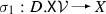 and
and  given by \(\sigma _1=k_1\,\circ \,{{\textsf {acInc} } (G)}{.}{{\textsf {X} }}_{\mathcal {V}} \,\circ \, {b_1}{.}{{\textsf {X} }}_{\mathcal {V}} \) and \(\sigma _2=k_2\circ {{\textsf {acInc} } (H)}{.}{{\textsf {X} }}_{\mathcal {V}} \circ {b_2}{.}{{\textsf {X} }}_{\mathcal {V}} \).
 -
(4)
We move the ACs \({\rho }{.}{{\textsf {ac} }} \) and \({G}{.}{{\textsf {ac} }} \) to the variable namespace set X by applying \(\sigma _{ VX }\) and \(k_1\). We then construct the AC \(\gamma \) over X as the conjunction of the three ACs that we constructed for the variables in X.
-
(5)
To obtain the AC for the graph H from \(\gamma \), we first hide the unprimed variables that originate from G using existential quantification. The resulting AC \(\exists k_1({G}{.}{{\textsf {X} }}).\;\gamma \) has free variables that are contained in X and that originate from H. We revert the (injective) function \(k_2\) to obtain the partial function \({\textsf {rev} } (k_2) \), which is defined on the free variables of \(\exists k_1({G}{.}{{\textsf {X} }}).\;\gamma \). We then obtain the AC \({\textsf {rev} } (k_2) (\exists k_1({G}{.}{{\textsf {X} }}).\;\gamma )\) as an AC over the variables of H. Note that when G and H share variables (i.e., \({G}{.}{{\textsf {X} }} \cap {H}{.}{{\textsf {X} }} \ne \varnothing \)), this last step may involve an implicit renaming (\(\alpha \)-conversionFootnote 25) of bound variables. Finally, we allow for a simplification of the obtained AC up to equivalence to ensure that our step relation defines resulting graphs up to isomorphism as usual. Also, applying equivalence here allows for the simplification of the AC, which may result in an AC where the added existential quantification is then removed.
-
(6)
To ensure that the resulting graph H describes a nonempty set of grounded graphs, we check whether the AC of H computed before is satisfiable. This requirement also guarantees that the part of \({\rho }{.}{{\textsf {ac} }}\) that is supposed to restrict rule applicability by referring to variables in G is properly checked.
 of
of  and
and  by adding the identity map
  when X is chosen as a comparison object with the two maps
  and
and  .
. and
and  given by
 These two stages for transforming the graph part and the AC part are formally defined in the items (1) and (2) of the definition below. See Fig. 11b and Fig. 11c for accompanying visualizations.
Definition 18
(Steps) If
-
(1)
-
\({\textsf {sat} }_{\exists } ({G}{.}{{\textsf {ac} }}) \),
-
\(\rho \in \mathcal {S}^{\mathsf {rules}} \) is a rule,
-
 ,
,\(m_1\models _{\mathsf {BGC}} {\rho }{.}{{\textsf {lC} }} \),
-
 ,
,\({\textsf {acInc} } (G) \circ c_1=m_1\),
-
 ,
, ,
, ,
, -
 ,
, ,
,\((c_2,b_2)~\text {is a pushout of}~({\rho }{.}{{\textsf {add} }},d) \),
-
 ,
,\({\textsf {acInc} } (H) \circ c_2=m_2\),
-
\(m_2\models _{\mathsf {BGC}} {\rho }{.}{{\textsf {rC} }} \),
-
-
(2)
-
 ,
, ,
, ,
, -
 is obtained by using the universal property of the coproduct \({\amalg } ({\rho }{.}{{\textsf {lX} }},{\rho }{.}{{\textsf {rX} }}) \),
 -
\(\gamma _{ eq }=\wedge \{\sigma _1(x)= \sigma _2(x) \mid x\in {D}{.}{{\textsf {X} }}-{d}{.}{{\textsf {X} }} ({K}{.}{{\textsf {X} }})\} \)
where \(\sigma _1=k_1\circ {{\textsf {acInc} } (G)}{.}{{\textsf {X} }}_{\mathcal {V}} \circ {b_1}{.}{{\textsf {X} }}_{\mathcal {V}} \)
\(\quad \,\hbox {and}\,\, \sigma _2=k_2\circ {{\textsf {acInc} } (H)}{.}{{\textsf {X} }}_{\mathcal {V}} \circ {b_2}{.}{{\textsf {X} }}_{\mathcal {V}} \),
-
\(\gamma = \wedge \{ \sigma _{ VX }({\rho }{.}{{\textsf {ac} }}), k_1({G}{.}{{\textsf {ac} }}), \gamma _{ eq } \} \) is an AC,
-
\({\textsf {sat} }_{\forall } ( {H}{.}{{\textsf {ac} }} \leftrightarrow {\textsf {rev} } (k_2) (\exists k_1({G}{.}{{\textsf {X} }}) .\; \gamma ) ) \), and
-
\({\textsf {sat} }_{\exists } ({H}{.}{{\textsf {ac} }}) \),
-
 ,
, ,
, ,
, ,
, ,
, ,
, ,
, ,
, ,
, ,
, ,
, is obtained by using the universal property of the coproduct
 then  is the step transforming the graph G into the graph H using the step label \(\varsigma = ( {\varsigma }{.}{{\textsf {rule} }}, {\varsigma }{.}{{\textsf {match} }}, {\varsigma }{.}{{\textsf {comatch} }}, {\varsigma }{.}{{\textsf {del} }}, {\varsigma }{.}{{\textsf {add} }})\in \mathcal {S}^{\mathsf {steps}} \) satisfying \({\varsigma }{.}{{\textsf {rule} }} =\rho \), \({\varsigma }{.}{{\textsf {match} }} =m_1\), \({\varsigma }{.}{{\textsf {comatch} }} =m_2\), \({\varsigma }{.}{{\textsf {del} }} ={\textsf {acInc} } (G) \circ b_1\), and \({\varsigma }{.}{{\textsf {add} }} ={\textsf {acInc} } (G) \circ b_1\).
The definition of steps above covers the general case as visualized in Fig. 11b. Note that the resulting diagram is no DPO diagram since e.g. \({L}{.}{{\textsf {ac} }} ={D}{.}{{\textsf {ac} }} =\top \) would require that \({G}{.}{{\textsf {ac} }} =\top \) as well. In our tool-based implementation, we can simplify the construction of \({H}{.}{{\textsf {ac} }} \) because we (a) do not change the name of variables that are not matched by \(c_1\), (b) use fresh names for preserved variables, and (c) use fresh names for created variables. In this case, we can assume that \(\gamma _{ eq }=\top \) and that \(k_1\) and \({\textsf {rev} } (k_2) \) do not need to be applied. For an example of a simple transformation step, consider Fig. 10b and Fig. 10c for the graph part and the AC part.
5.2 (Timed) graph transformation sequences
We now define graph transformation sequences that can be obtained by performing a finite or an infinite number of steps using rules. However, we only provide the underlying data structure of graph sequences in the definition below and do not yet connect the notions of steps and graph sequences at this point. Such a graph sequence is defined as a mapping of indices from the set B to spans of morphisms where adjacent spans must have a common graph as end point and start point, i.e., the graph \(G_1\) is such a common start and end point of the two spans  and
and  in Fig. 25a on page 32).

The type graph \( TG \) and the initial graph \(G_0\) for the timed graph transformation system from Example 2. a The type graph \( TG \) for our running example where the attributes cts and dts are used later on by the operation \({\textsf {Fold} }\). Intuitively, tasks run on a system and the execution of a task leads to the corresponding computed result at the system. We assume that there is a unique system on which up to limit-many further tasks may be spawned. Execution of a task requires a duration of type :dur that is nondeterministically generated when the task is spawned. Results contain an attribute value and are associated to the task from which they originate via their attribute id. When the system has a loop of type :active, it is in the scheduling mode where it assigns a loop of type :slot to each of the tasks. A unique attribute time of a system connected is used to represent the current global time. Free variables of type :x are used in rules to nondeterministically select values for the id and dur attributes. b The initial graph \(G_0\) containing an empty system without tasks and results. The current global time is given by the attribute time of the system, which is set to the initial value of 0
Definition 19
(Graph Sequences) If \(G_0\in \mathbf {Graphs} \) is a graph, \(n\in \mathbf {N} \cup \{\infty \}\) is a length, and \(B=\{k\in \mathbf {N} \mid k<n\}\) is the set of indices from 0 to \(n-1\) (note that B is empty for \(n=0\)), then  is a graph sequence of length n over \(G_0\), written \(\pi \in \Pi _{G_0} \), and \({\textsf {length} }(\pi ) =n\), if both items apply.Footnote 26
-
\(0\in B\) and
 imply that \(G=G_0\).
 -
 .
.
 imply that
  .
.Moreover, we define the following abbreviations and operations.
-
\(\Pi ^{\mathsf {fin}}_{G_0} =\{\pi \in \Pi _{G_0} \mid {\textsf {length} }(\pi ) \ne \infty \}\) is the class of all finite graph sequences over \(G_0\).
-
If \(\pi \in \Pi ^{\mathsf {fin}}_{G_0} \) is a finite graph sequence over \(G_0\) and \({\textsf {length} }(\pi ) =0\), then \(\pi \) is empty, written \(\pi =\lambda \) (for the empty word \(\lambda \)).
-
If \(\pi \in \Pi ^{\mathsf {fin}}_{G_0} \) is a finite graph sequence over \(G_0\), \({\textsf {length} }(\pi ) =n\), H is a graph, \(k\le n\), (\(k=0\) implies \(G_0=H\)), and (\(k>0\) implies
 ), then \(\pi \) starts with \(G_0\) and ends with H after k steps, written \(\pi ^{\mathsf {G}}(k) =H\).
 -
If \(\pi \in \Pi ^{\mathsf {fin}}_{G_0} \) is a finite graph sequence over \(G_0\), \({\textsf {length} }(\pi ) =n\), and \(\pi ^{\mathsf {G}}(n) =H\), then \(\pi \) starts with \(G_0\) and ends with H, written \(\pi \in \Pi ^{\mathsf {fin}}_{G_0,H} \).
-
If \(\pi \in \Pi ^{\mathsf {fin}}_{G_0,H} \) is a finite graph sequence starting with \(G_0\) and ending with H, \({\textsf {length} }(\pi ) =n\), and \(\pi '=\{(n-(k+1),(r,\ell ))\mid (k,(\ell ,r))\in \pi \}\in \Pi ^{\mathsf {fin}}_{H,G_0} \) is the finite graph sequence starting with H and ending with \(G_0\) obtained from \(\pi \), then \(\pi '\) is the reversal of \(\pi \), written \({\textsf {rev} }(\pi ) =\pi '\).
 ), then
Rules for the timed graph transformation system from Example 2 (the remaining rules are given in Fig. 14). a The rule \(\rho _{ SpawnTask }\) for adding a task to a system with a loop of type :slot indicating that the task has the permission to run immediately. The global variable w is used in the AC of the rule to choose an integer for the id attribute of the task from the interval \([0,5]\). The application condition of the rule requires that no task with the chosen id is already attached to the system. The global variable \(v'\) is used in the AC of the rule to choose an integer from the interval \([1,10]\), which is then multiplied by 100, for the dur attribute of the task. Note that the execution of tasks requires much more time compared to the other operations of the system. Also, the AC of the rule states that one time unit elapses when this rule is applied and that the limit attribute of the system is decremented from a value strictly greater than 0. Note that this rule does not check that there is no left-over result for the id that is chosen for the new task. We will detect this as a violation by our testing approach later on. b The rule \(\rho _{ StepTask }\) reduces the remaining duration of a task that is connected to a system by 100. The loop of type \({\text {:slot}}\) on the task is required to run the task. This loop exists because the system assigned a slot to the task in the past and is then removed by rule application. The application condition of the rule requires that the system has no loop of type \({\text {:active}}\), which means that the system is not in the scheduling mode. Moreover, the AC of the rule states that 100 time units elapse when this rule is applied. c The rule \(\rho _{ StepTaskEnd }\) removes a task from a system, when its execution has finished (indicated by the remaining duration of 100 that is reduced to 0 by rule application), and adds a result with the same id attribute to the system. The computed result stores a value that is always \( ok \) for simplicity. The loop of the type \({\text {:slot}}\) on the task is required for the task to run and to terminate. The application condition of the rule requires that the system has no loop of type \({\text {:active}}\), which means that the system is not in the scheduling mode. Moreover, the AC of the rule states that 100 time units elapse when this rule is applied

Rules for the timed graph transformation system from Example 2 (the remaining rules are given in Fig. 13). a The rule \(\rho _{ ConsumeResult }\) removes a result, which was previously computed, from a system. The delivery of the result to the user is not explicitly modeled in this rule. The AC of the rule states that one time unit elapses when this rule is applied. b The rule \(\rho _{ StartScheduling }\) initiates the scheduling mode for a system with at least one task by adding a loop of type :active to the system. The application condition ensures that no task (also not the task T of the left-hand side graph) has a remaining loop of type :slot that renders that task eligible to run and that the system is not already active. The AC of the rule states that one time unit elapses when this rule is applied. c The rule \(\rho _{ Schedule }\) adds a loop of type :slot to a task that is connected to a system in scheduling mode. The application condition ensures that the task has not yet an assigned loop of type :slot. The AC of the rule states that one time unit elapses when this rule is applied. d The rule \(\rho _{ StopScheduling }\) terminates the scheduling mode for the system by removing the loop of type :active. The application condition ensures that there is no task without a loop of type :slot. The AC of the rule states that one time unit elapses when this rule is applied

A TGS and its GH for the timed graph transformation system from Example 2. a A TGS \(\pi \) in which two results with the same id attribute are generated. b The GH obtained from folding the TGS from a
In the following, we introduce timed graph sequences (TGSs) where each step consumes a positive amount of time. To operate on a TGS, we obtain the total time that has passed up to some point in the TGS by retrieving the total time from graphs in the TGS. For this purpose, we assume that the total time is stored in the graphs of the TGS e.g. in variables that are restricted by the ACs of the graphs. The total time stored in such a variable must then be increased in each graph transformation step by including such an increase in each rule of the timed graph transformation system. Note that graphs cannot occur more than once in a TGS because time must strictly increase but, apart from the stored total time, graphs may very well coincide as usual.Footnote 27 In the definition below, we abstract from a particular encoding for the total time and assume a partial function \( time \) that returns a strictly increasing sequence of total timepoints from  (the set of all real numbers greater or equal to 0), which diverges for infinite TGSs when being applied to the graphs in a TGS.
Definition 20
(Timed Graph Sequences (TGSs)) If
-
\(\pi \in \Pi _{G_0} \) is a graph sequence over \(G_0\),
-
 is a partial function,
 -
\( time (G_0) =0\),
-
\(\forall k<{\textsf {length} }(\pi ).\; time (\pi ^{\mathsf {G}}(k)) \ne {\textsf {undef} } \),
-
\(\forall 0<k<{\textsf {length} }(\pi ). \; time (\pi ^{\mathsf {G}}(k-1)) < time (\pi ^{\mathsf {G}}(k)) \), and
-
if \({\textsf {length} }(\pi ) =\infty \), then
 ,
,
 is a partial function,
 ,
,then \(\pi \) is a timed graph sequence (TGS) over \(G_0\) w.r.t. the partial function \( time \), written \(\pi \in \Pi ^{ time }_{G_0} \).
Moreover, we define the following abbreviations and operations.
-
\(\Pi ^{\mathsf {fin}, time }_{G_0} =\Pi ^{\mathsf {fin}}_{G_0} \cap \Pi ^{ time }_{G_0} \) is the set of all finite TGSs that start in \(G_0\).
-
\(\Pi ^{\mathsf {fin}, time }_{G_0,H} =\Pi ^{\mathsf {fin}, time }_{G_0} \cap \Pi _{G_0,H} \) is the set of all finite TGSs that start in \(G_0\) and end in H.
-
If \(\pi \in \Pi ^{\mathsf {fin}, time }_{G_0,H} \) is a finite TGS that starts in \(G_0\) and ends in H and \( time (H) =t\), then t is the duration of \(\pi \), written \({\textsf {dur} }(\pi ) =t\).
-
If \(\pi \in \Pi ^{ time }_{G_0} \) is a TGS starting in \(G_0\),
 is a total timepoint, \({\textsf {length} }(\pi ) =n\), \(k=\min \{k<n\mid time (\pi ^{\mathsf {G}}(k)) \ge t\} \cup \{n-1\mid n\ne \infty \}\), and \(\pi ^{\mathsf {G}}(k) =H\), then \(\pi \) is in the graph H at the total timepoint t and index k w.r.t. the partial function \( time \), written \(\pi ^{\mathsf {T}}(t) =H\) or \(\pi ^{\mathsf {T}}(t) =k\).
 -
If \(\pi \) and \(\pi '\) are TGSs from \(\Pi ^{ time }_{G_0} \), \(t_1\) and \(t_2\) are total timepoints from
 , \(t_1\le t_2\), \(\pi ^{\mathsf {T}}(t_1) =k_1\), \(\pi ^{\mathsf {T}}(t_2) =k_2\), and \(\pi '=\{(k,x)\mid (k+k_1,x)\in \pi ,k+k_1\le k_2\}\), then \(\pi '\) is the TGS contained in \(\pi \) between the total timepoints \(t_1\) and \(t_2\) w.r.t. the partial function \( time \), written \(\pi ^{\mathsf {T}}(\{t_1,t_2\}) =\pi '\).
 is a total timepoint,
  ,
, Consider Fig. 15a where the partial function \( time \) can be defined to extract the value of the \(\text {time} \) attribute of the node S. Hence, the total time would be increased by 1, 100, 1, and 100 in the depicted spans.
5.3 (Timed) graph transformation systems
We now connect the notion of steps introduced in Definition 18 with the notion of (timed) graph sequences from above by means of (timed) graph transformation systems that generate (timed) graph sequences.
Graph transformation systems, which contain a finite set of finite rules R and a finite initial graph G, are introduced in the following definition.
Definition 21
(Graph Transformation Systems) If R is a finite set of finite rules from \(\mathcal {S}^{\mathsf {rules}} \) and \(G\in \mathbf {Graphs} \) is a finite graph, then \( S =(R,G)\) is a graph transformation system, written \( S \in \mathcal {S}^{\mathsf {gts}} \).
The graph sequences that can be derived from the initial graph of a graph transformation system are those graph sequences in which each span of morphisms can be justified by a step using one of the rules in R of the graph transformation system.
Definition 22
(Semantics of Graph Transformation Systems) If
-
\( S =(R,G)\in \mathcal {S}^{\mathsf {gts}} \) is a graph transformation system,
-
\(\pi \in \Pi _{G} \) is a graph sequence over G, and
-
for every \(k<{\textsf {length} }(\pi ) \) there is some step label \(\varsigma \in \mathcal {S}^{\mathsf {steps}} \) s.t.
 is a step,
  is a span of morphisms, and \({\varsigma }{.}{{\textsf {rule} }} \in R\) is a rule,
 is a step,
  is a span of morphisms, and
 then \(\pi \) is a graph sequence of S, written \(\pi \in \mathcal {S}^{\mathsf {gts\cdot s}}_{S} \).
Similarly to graph transformation systems, timed graph transformation systems contain a finite set of finite rules R and a finite initial graph G. As an additional component, timed graph transformation systems contain a partial function \( time \) for extracting the current global time from the derived graphs.
Definition 23
(Timed Graph Transformation Systems) If R is a finite set of finite rules from \(\mathcal {S}^{\mathsf {rules}} \), \(G\in \mathbf {Graphs} \) is a finite graph, and  is a partial function, then \( S =(R,G, time )\) is a timed graph transformation system, written \( S \in \mathcal {S}^{\mathsf {tgts}}_{ time } \).
The timed graph sequences of timed graph transformation systems are constructed as for graph transformation systems above. Recall that the partial function \( time \) is only used for postprocessing of already derived TGSs.
Definition 24
(Semantics of Timed Graph Transformation Systems) If \( S =(R,G, time )\in \mathcal {S}^{\mathsf {tgts}}_{ time } \) is a timed graph transformation system \(\pi \in \mathcal {S}^{\mathsf {gts\cdot s}}_{(R,G)} \) is a graph sequence of the graph transformation system (R, G), and \(\pi \in \Pi ^{ time }_{G} \), then \(\pi \) is a TGS of S, written \(\pi \in \mathcal {S}^{\mathsf {tgts\cdot s}}_{S} \).
With these definitions in place, we now present an example of a timed graph transformation system that is used in Sect. 7 and Sect. 8 later on.
Example 2
(Running Example of a Timed Graph Transformation System for Task Execution and Scheduling) For this example of a timed graph transformation system, we use the type graph \( TG \) from Fig. 12a, the initial graph \(G_0\) from Fig. 12b, and the rules from Fig. 13 and Fig. 14. In this example, we slightly adapt our visual notation for rules. We use the same unprimed variable names (such as x) in the graphs L, K, and R when the AC of the rule requires that the variable remains unchanged (in the sense of \(x'= x \) for \(x'\in {R}{.}{{\textsf {X} }} \)), instead of distinguishing between unprimed and primed variables as stated in Notation 2. The partial function \( time \) is defined to extract the value of the local variable \(x_{ tp }\) connected to the unique time attribute of the unique system contained in each derived graph. The value of this local variable \(x_{ tp }\) is increased by each rule application. See Fig. 15a for an example of a TGS generated from this timed graph transformation system. In this TGS two tasks with the same id are executed sequentially leading to duplicate result nodes because the result node of the first task is not consumed before the second task is finished (see also Fig. 34 on page 47 where the presence of such a result node with the same id is excluded in the application condition).
6 Graph logic
We now extend the basic graph logic BGL from Sect. 4 with the novel operator \(\Delta \) (called delta) that relies on so-called restriction-extension patterns to obtain the graph logic GL. The notions of restriction-extension patterns and rules from Definition 16 are technically identical but the two morphisms \({\rho }{.}{{\textsf {del} }} \) and \({\rho }{.}{{\textsf {add} }} \) are referred to by \({\rho }{.}{{\textsf {res} }} \) and \({\rho }{.}{{\textsf {ext} }} \) instead.
Definition 25
(Restriction-Extension Pattern) A tuple \(\rho =({\rho }{.}{{\textsf {res} }},{\rho }{.}{{\textsf {ext} }},{\rho }{.}{{\textsf {lX} }},{\rho }{.}{{\textsf {rX} }},{\rho }{.}{{\textsf {ac} }},{\rho }{.}{{\textsf {lC} }},{\rho }{.}{{\textsf {rC} }})\) is a restriction-extension pattern, written \(\rho \in \mathcal {S}^{\mathsf {REP}} \), if
-
L, K, and R are graphs,
-
 ,
, -
 are monomorphisms,
 -
 is a coproduct,
 -
\({\rho }{.}{{\textsf {ac} }} \in \mathcal {S}^{{\textsf {AC} }} _{V} \) is an AC,
-
\({\rho }{.}{{\textsf {lC} }} \in \mathcal {S}^{\mathsf {BGC}} _{L} \),
-
\({\rho }{.}{{\textsf {rC} }} \in \mathcal {S}^{\mathsf {BGC}} _{R} \) are BGCs,Footnote 28 and
-
\({L}{.}{{\textsf {ac} }} ={K}{.}{{\textsf {ac} }} ={R}{.}{{\textsf {ac} }} =\top \).
 ,
, are monomorphisms,
 is a coproduct,
Moreover, we define the following abbreviations.
-
\({\rho }{.}{{\textsf {lG} }} =L\) is the left-hand side graph of the restriction-extension pattern \(\rho \).
-
\({\rho }{.}{{\textsf {rG} }} =R\) is the right-hand side graph of the restriction-extension pattern \(\rho \).
The delta operator of GL combines restriction and extension as in the restrict and exists operators of BGL. While the delta operator does not increase the expressiveness, as shown by encoding the delta operator later on using BGL operators only, it certainly increases the descriptive expressiveness of GL compared to BGL because properties can be stated using exponentially smaller conditions when using the delta operator. Note that the operator restrict has been added to BGL for the same reason of improving its applicability by allowing for more concise conditions. In particular, the delta operator permits to first restrict a current match and then to extend the restricted match in a way such that attribute values from before the restriction can be used to specify the extension. The similar coupling of removal and addition is also a major benefit of span-based DPO graph transformation, which allows to add graph elements and to specify the AC of the resulting graph on the basis of the context established by the removal of graph elements.
Definition 26
(Graph Conditions (GCs)) If \(H\in \mathbf {Graphs} \) is a graph, then \(\bar{\phi }\in \mathcal {S}^{\mathsf {GC}} _{H} \) is a graph condition (GC) over H, if one of the following items applies.
- \(\bullet \):
-
\(\bar{\phi }=\wedge S \) and \(S\mathrel {\subseteq _{\mathsf {fin}}} \mathcal {S}^{\mathsf {GC}} _{H} \).
- \(\bullet \):
-
\(\bar{\phi }=\lnot \phi \) and \(\phi \in \mathcal {S}^{\mathsf {GC}} _{H} \).
- \(\bullet \):
-
 and \(\phi \in \mathcal {S}^{\mathsf {GC}} _{H'} \).
 - \(\bullet \):
-
 and \(\phi \in \mathcal {S}^{\mathsf {GC}} _{H'} \).
 - \(\bullet \):
-
\(\bar{\phi }=\Delta ^{}(\rho ,\phi ) \),
 and
and  and
and - \(\bullet \):
-
\(\rho \in \mathcal {S}^{\mathsf {REP}} \) is a restriction-extension pattern,
- \(\bullet \):
-
\({\rho }{.}{{\textsf {lG} }} =H\),
- \(\bullet \):
-
\({\rho }{.}{{\textsf {rG} }} =H'\), and
- \(\bullet \):
-
\(\phi \in \mathcal {S}^{\mathsf {GC}} _{H'} \) is a GC over \(H'\).
Moreover, we define the following abbreviations.
-
true: \(\top =\wedge \varnothing \)
-
false: \(\bot =\lnot \top \)
-
disjunction: \(\vee S =\lnot (\wedge \{\lnot \phi \mid \phi \in S\}) \)
-
universal quantification: \(\forall (f,\phi ) =\lnot \exists (f,\lnot \phi ) \)
-
delta-forall: \(\Delta ^{\mathsf {A}}(\rho ,\phi ) =\lnot (\Delta ^{}(\rho ,\lnot \phi )) \)
-
delta-existsFootnote 29: \(\Delta ^{\mathsf {E}}(\rho ,\phi ) =\Delta ^{}(\rho ,\phi ) \)
See Fig. 16a for an example of a GC where we employ the following notation for restriction-extension patterns occurring in GCs.
Notation 3
(Restriction–Extension Patterns in GCs) We adapt our notation for BGCs from Notation 1 as follows. For the delta operator, we depict a GC \(\bar{\phi }=\Delta ^{}(\rho ,\phi ) \) in three compartments separated by vertical lines assuming that \({\rho }{.}{{\textsf {res} }} \) and \({\rho }{.}{{\textsf {ext} }} \) are inclusion morphisms. We depict the morphism \({\rho }{.}{{\textsf {res} }} \), by employing the notation for monomorphisms used in a restrict operator, in the first compartment. We depict the morphism \({\rho }{.}{{\textsf {ext} }} \), by employing the notation for monomorphisms used in an exists operator, in the second compartment. Lastly, we depict \({\rho }{.}{{\textsf {ac} }}\) in the third compartment. If \({\rho }{.}{{\textsf {res} }} \) or \({\rho }{.}{{\textsf {ext} }} \) is an identity morphism, we denote this by \({\textsf {id} } \). If \({\rho }{.}{{\textsf {res} }} \) is an initial morphism from the empty graph, we denote this by \(\varvec{\varnothing } \). If \({\rho }{.}{{\textsf {res} }} \) or \({\rho }{.}{{\textsf {ext} }} \) is not an inclusion morphism or one of the application conditions \({\rho }{.}{{\textsf {lC} }}\) or \({\rho }{.}{{\textsf {rC} }}\) is not \(\top \), we use our more general notation for rules from Notation 2.
The definition of the satisfaction relation of GL follows the definition of the satisfaction relation of BGL when the GC uses the conjunction, negation, exists, or restrict operators. For the additional operator delta, we proceed as for restrict and exists to obtain for a given match  a resulting match
  . We then check in addition whether the AC \({\rho }{.}{{\textsf {ac} }}\) is satisfied by the host graph once it is translated using m and \(m'\) to the namespace given by the variables of the graph. See Fig. 16c where we give an example for checking GC satisfaction.
Definition 27
(Satisfaction of GCs) If \(\bar{\phi }\in \mathcal {S}^{\mathsf {GC}} _{H} \) is a GC and  is a partially injective morphism, then \(m\models _{\mathsf {GC}} \bar{\phi } \), if one of the following items applies.
- \(\bullet \):
-
\(\bar{\phi }=\wedge S \) and \(\forall \phi \in S.\;m\models _{\mathsf {GC}} \phi \).
- \(\bullet \):
-
\(\bar{\phi }=\lnot \phi \) and \(m\not \models _{\mathsf {GC}} \phi \).
- \(\bullet \):
-
 and there is
  s.t. \(m=m'\circ f\) and \(m'\models _{\mathsf {GC}} \phi \).
 - \(\bullet \):
-
 and \(m\circ f\models _{\mathsf {GC}} \phi \).
 - \(\bullet \):
-
\(\bar{\phi }=\Delta ^{}(\rho ,\phi ) \) and there is some
 s.t.
s.t.
 and there is
  s.t.
s.t.  and
and  s.t.
s.t.- \(\bullet \):
-
\(m\circ {\rho }{.}{{\textsf {res} }} =m'\circ {\rho }{.}{{\textsf {ext} }} \),
- \(\bullet \):
-
\(m\models _{\mathsf {BGC}} {\rho }{.}{{\textsf {lC} }} \),
- \(\bullet \):
-
\(m'\models _{\mathsf {BGC}} {\rho }{.}{{\textsf {rC} }} \),
- \(\bullet \):
-
 maps to the set V of variables over which \({\rho }{.}{{\textsf {ac} }} \) is defined,
 - \(\bullet \):
-
 is the unique mapping induced by the universal property of the coproduct of the restriction-extension pattern where we use the two maps \({m}{.}{{\textsf {X} }} \) and \({m'}{.}{{\textsf {X} }} \) leading to the set \({G}{.}{{\textsf {X} }} \cup \mathcal {V} \) for comparison,
 - \(\bullet \):
-
\({\textsf {sat} }_{\forall } ({G}{.}{{\textsf {ac} }} \rightarrow \sigma _{ VG }({\rho }{.}{{\textsf {ac} }})) \), and
- \(\bullet \):
-
\(m'\models _{\mathsf {GC}} \phi \).
 maps to the set V of variables over which
  is the unique mapping induced by the universal property of the coproduct of the restriction-extension pattern where we use the two maps
 Also, if \(\bar{\phi }\in \mathcal {S}^{\mathsf {GC}} _{\varvec{\varnothing }} \) and \({\textsf {i} } (G) \models _{\mathsf {GC}} \bar{\phi } \), then \(G\models _{\mathsf {GC}} \bar{\phi } \).

Example of a GC, GC satisfaction, and the operation \({\textsf {enc} }_{\Delta }\). a A GC  where
where  ,
,  , and \({\rho }{.}{{\textsf {ac} }} =\wedge \{ x= 0, 2\le y, z'= y+ 1 \} \) (cf. c for a visualization of the contained morphisms \(f_0\), \(f_1\), and \(f_2\)). This GC formalizes the property “There are connected nodes \(a{\text {:A}}\) and \(b{\text {:B}}\) with id attributes such that, when restricting the match to the node a only, there is also a node \(c{\text {:C}}\) with an id attribute connected to the node a. Also, the id attributes of a, b and c must satisfy the given AC.” b A graph G satisfying the GC \(\phi \) from b. c For checking the satisfaction of the GC \(\phi \) from a by the graph G from b, we use the initial morphism \(m_0={\textsf {i} } (G) \), extend that morphism according to \(f_0\) to the match \(m_1\), restrict and then extend \(m_1\) to the match \(m_2\) and then trivially observe that \(m_2\) satisfies the remaining subcondition \(\top \). Moreover, we verify that \({G}{.}{{\textsf {ac} }} =\wedge \{\bar{x}= 0,\bar{y}= 4,\bar{z}= 5 \} \) always implies the translated AC of the evolution pattern \(\wedge \{\bar{x}= 0,2\le \bar{y},\bar{z}= \bar{y}+ 1 \} \). d The BGC obtained from the GC \(\phi \) given in a using the operation \({\textsf {enc} }_{\Delta }\) from Definition 28
Note that the graph H in Definition 26 above must have the AC \(\top \) for the delta operator according to the definition of restriction-extension patterns above. Hence, the delta operator must be combined with the other operators exists and restrict with care. That is,  can only be a valid GC when \({\rho }{.}{{\textsf {res} }} \) has the codomain H and \({H}{.}{{\textsf {ac} }} =\top \).
We now introduce an encoding operation \({\textsf {enc} }_{\Delta }\) for the translation of GCs into equivalent BGCs to show that BGL is as expressive as GL (the reverse direction holds trivially because all BGCs are GCs and the satisfaction relations of BGL and GL agree on the BGL operators). Note that this encoding operation results, as for the encoding of the restrict operator in Definition 15, in an exponential blowup of the size of the condition at hand due to the usage of the operation \({\textsf {overlap} }\) from Definition 11.
The encoding of the delta operator is similar to the equivalence of span-based and cospan-based DPO transformations as follows. In the cospan-based DPO approach [30], rules are given by cospans instead of spans as in the more common span-based DPO approach in [29]. Both approaches are equivalent [30] because equivalent span rules and cospan rules are constructed from each other using the pullback and pushout of the cospan rules and span rules, respectively. Intuitively, cospan rules  describe the addition of graph elements using \(\ell \) and then the removal of graph elements using r, which is the reverse interpretation compared to span rules. That is, the order of addition and removal of graph elements is swapped between the two approaches. See Fig. 17 for an example of the pushout/pullback-based conversion between span rules and cospan rules that are equivalent w.r.t. DPO transformation.
Similarly, when applying our operation \({\textsf {enc} }_{\Delta }\) defined below to a GC \(\bar{\phi }=\Delta ^{}(\rho ,\phi ) \), we want to exchange the restriction \({\rho }{.}{{\textsf {res} }} \) and the extension \({\rho }{.}{{\textsf {ext} }} \) to be able to use first the operator exists and then the operator restrict afterwards. The described exchange is needed because when the restrict operator is used first, we lose information about values of variables that are dropped from the match. This information would then be missing when extending the match afterwards using the exists operator. For the GC \(\bar{\phi }=\Delta ^{}(\rho ,\phi ) \), we have the span \(({\rho }{.}{{\textsf {res} }},{\rho }{.}{{\textsf {ext} }})\) given but construct all overlappings \(K'\) (see Fig. 18) instead of only computing the pushout of \(({\rho }{.}{{\textsf {res} }},{\rho }{.}{{\textsf {ext} }})\), which is one of these overlappings. All constructed overlappings are needed because the GC satisfaction relation permits that graph elements that were removed from the match according to \({\rho }{.}{{\textsf {res} }}\) are rematched for \({\rho }{.}{{\textsf {ext} }}\) afterward. In comparison, deleted and then created graph elements are assumed to be different by default in DPO graph transformation. See Fig. 17 for an example where all overlappings are created for a span rule. An example for \({\textsf {enc} }_{\Delta }\) for the case without ACs is given in Fig. 19.
In addition to the described exchange of restriction and extension of matches, we also adapt the AC of the given rule \(\rho \) by renaming the variables appropriately. Since \(\rho \) is a restriction-extension pattern (see Fig. 18 for a visualization), we know that  is a coproduct, which implies that we obtain a unique variable substitution \(\sigma \) from V to the set of variables \({K'}{.}{{\textsf {X} }} \) of the overlapping graph \(K'\) constructed before (as in the satisfaction relation for GL). We then obtain the graph \(K''\) from the overlapping graph \(K'\) by assigning the AC of the restriction-extension pattern to it after applying the variable substitution \(\sigma \). For the following definition of the operation \({\textsf {enc} }_{\Delta }\), see Fig. 18 for an accompanying visualization, see Fig. 16d for an application to the already considered GC from Fig. 16a with one overlapping and ACs, and see Fig. 19 for an application to a GC without ACs relying on the two overlappings given in Fig. 17a.

Construction of overlappings for the operation \({\textsf {enc} }_{\Delta }\) and relationship between span-based DPO steps and cospan-based DPO steps. a A span \(({\rho }{.}{{\textsf {res} }},{\rho }{.}{{\textsf {ext} }})\) and the overlappings \((f_1,f_2)\) and \((g_1,g_2)\) computed by the operation \({\textsf {overlap} } ({\rho }{.}{{\textsf {res} }},{\rho }{.}{{\textsf {ext} }}) \) from Definition 11 such that \((g_1,g_2)\) is the pushout of \(({\rho }{.}{{\textsf {res} }},{\rho }{.}{{\textsf {ext} }})\) and \(({\rho }{.}{{\textsf {res} }},{\rho }{.}{{\textsf {ext} }})\) is the pullback of \((g_1,g_2)\). b A DPO transformation step using the rule span \(({\rho }{.}{{\textsf {res} }},{\rho }{.}{{\textsf {ext} }})\) from a where \(a_1\) is removed before \(a_2\) and \(e_2\) are added. c A DPO transformation step using the cospan rule \((g_1,g_2)\) from a where \(a_2\) and \(e_2\) are added before \(a_1\) is removed
Definition 28
(Operation \({\textsf {enc} }_{\Delta }\) ) If \(\bar{\phi }\in \mathcal {S}^{\mathsf {GC}} _{H} \) is a GC over H and \(\bar{\phi }'\in \mathcal {S}^{\mathsf {BGC}} _{H} \) is a BGC over H, then \({\textsf {enc} }_{\Delta } (\bar{\phi }) =\bar{\phi }'\), if one of the following items applies.
- \(\bullet \):
-
\(\bar{\phi }=\wedge S \) and \(\bar{\phi }'=\wedge \{{\textsf {enc} }_{\Delta } (\phi ) \mid \phi \in S\} \).
- \(\bullet \):
-
\(\bar{\phi }=\lnot \phi \) and \(\bar{\phi }'=\lnot {\textsf {enc} }_{\Delta } (\phi ) \).
- \(\bullet \):
-
 and \(\bar{\phi }'=\exists (f,{\textsf {enc} }_{\Delta } (\phi )) \).
 - \(\bullet \):
-
 and \(\bar{\phi }'=\nu (f,{\textsf {enc} }_{\Delta } (\phi )) \).
 - \(\bullet \):
-
\(\bar{\phi }=\Delta ^{}(\rho ,\phi ) \),
the set S used below contains all cospans of the form
 that satisfy the following items:
 - \(\bullet \):
-
for the graph part:
- \(\bullet \):
-
 ,
, - \(\bullet \):
-
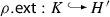 are monomorphisms,
 - \(\bullet \):
-
 is an overlapping,
- \(\bullet \):
-
for the AC part:
- \(\bullet \):
-
 ,
, - \(\bullet \):
-
 are maps identifying the variables in the coproduct V,
 - \(\bullet \):
-
 is the unique mapping induced by the universal property of the coproduct of the restriction-extension pattern where \((\ell ',r')\) are used for comparison,
 - \(\bullet \):
-
 is an AC inclusion morphism, and
 - \(\bullet \):
-
\({K''}{.}{{\textsf {ac} }} =\sigma ({\rho }{.}{{\textsf {ac} }})\) and
 for the application conditions \({\rho }{.}{{\textsf {lC} }} \) and \({\rho }{.}{{\textsf {rC} }} \).Footnote 30
 and
and  and
and  that satisfy the following items:
  ,
, are monomorphisms,
 is an overlapping,
 ,
, are maps identifying the variables in the coproduct V,
 is the unique mapping induced by the universal property of the coproduct of the restriction-extension pattern where
  is an AC inclusion morphism, and
 for the application conditions
Visualization for Definition 28
We now state that the translation of GCs into BGCs is sound w.r.t. the corresponding satisfaction relations.
Theorem 4
(Soundness of \({\textsf {enc} }_{\Delta }\)) If \(\phi \in \mathcal {S}^{\mathsf {GC}} _{H} \) is a GC and  is a partially injective morphism, then \(m\models _{\mathsf {GC}} \phi \) iff \(m\models _{\mathsf {BGC}} {\textsf {enc} }_{\Delta } (\phi ) \).
See page 70 for the proof of this theorem.
The encoding operation \({\textsf {enc} }_{\Delta }\) is also sound for graphs as a direct consequence of Theorem 4.
Corollary 2
(Soundness of \({\textsf {enc} }_{\Delta }\) for Graphs) If \(\phi \in \mathcal {S}^{\mathsf {GC}} _{\varvec{\varnothing }} \) is a GC and \(G\in \mathbf {Graphs} \) is a graph, then \(G\models _{\mathsf {GC}} \phi \) iff \(G\models _{\mathsf {BGC}} {\textsf {enc} }_{\Delta } (\phi ) \).
See page 72 for the proof of this corollary.
We conclude from this corollary that the operation \({\textsf {enc} }_{\Delta }\) can be used to translate the GC satisfaction problem into a BGC satisfaction problem. The operation \({\textsf {enc} }_{\Delta }\) is supported by our prototypical implementation in AutoGraph. Recall that satisfaction checking for the resulting BGC is also supported as well in AutoGraph by means of the encoding operation \({\textsf {enc} }_{\nu }\) (see Sect. 4) and \({\textsf {check} }_{\textsf {BGC} }\) (see “Appendix B”).
7 Metric temporal graph logic
We extend the graph logic GL for specifying graphs from before to the metric temporal graph logic MTGL for specifying TGSs. The integration of graph pattern matching from GL using the delta operator and the additional metric temporal operators allows for the formalization of more advanced metric temporal properties compared to [38, 81].
As a main concept, we first introduce an operation for propagating a given match (also called binding) of a graph into a given TGS at one timepoint to a graph in that sequence at another timepoint. This propagation is limited by evolution patterns used in conditions of MTGL for specifying modifications carried out in subsequences of the TGS at hand. Such a propagation of a match entails its partial preservation, its extension, and its restriction over several timed spans where values matched at the start and end of such a subsequence can be compared. We discuss this propagation operation in Subsect. 7.1. Afterwards in Subsect. 7.2, we introduce the syntax and semantics of MTGL relying on this operation for match propagation.
In Subsect. 7.3, we then introduce operations for folding a given TGS into a single graph called graph with history, which contains all the information represented by the TGS regarding the modifications given by timed spans and their total timepoints. Finally, in Subsect. 7.4, we introduce an encoding operation for translating a condition of MTGL into a condition of GL. Combining the folding of TGSs and the encoding of conditions of MTGL, we translate thereby the satisfaction problem into a GL satisfaction problem, which can be tackled more easily.

Example for the operation \({\textsf {enc} }_{\Delta }\) based on the overlapping computation from Fig. 17. a The GC \(\phi \) based on the span \(({\rho }{.}{{\textsf {res} }},{\rho }{.}{{\textsf {ext} }})\) from Fig. 17a. b The BGC \(\phi '\) obtained from the GC \(\phi \) given in a using the operation \({\textsf {enc} }_{\Delta }\) from Definition 28 incorporating the two overlappings given in Fig. 17a. Note that in the second line, we are using the monomorphisms \(f_1\) and \(f_2\) from Fig. 17a, which are no inclusion morphisms
7.1 Propagation of matches over timed graph sequences
To introduce the propagation of matches over TGSs, we first introduce the operation admissible-comatches. This operation takes a graph transformation span  ,Footnote 31 a match
  , and a (so-called) evolution pattern \(\theta \) with left- and right-hand side graphs L and R as inputs and then checks whether the changes given by the graph transformation span \((\ell ,r)\) are permitted by the evolution pattern \(\theta \) and returns a set of corresponding matches
  . In particular, the operation \({\textsf {admissible-comatches}}\) restricts the given match \(m_1\) according to the evolution pattern \(\theta \) (similarly to the BGC operator restrict), checks whether at least the deletions specified in the evolution pattern \(\theta \) are performed, checks whether at least the additions specified in the evolution pattern \(\theta \) are performed, and determines an extended match \(m_2\) according to the evolution pattern \(\theta \) (similarly to the BGC operator exists). That is, an evolution pattern describes that certain elements of the given match are not relevant, describes that certain elements must have been deleted and added, and that certain elements must be matchable.
This idea is similar to the concept of covariance and contravariance in programming languages. For example, an abstract function  (e.g. contained in a Java interface) can be implemented by a concrete function
  (e.g. in a class implementing the interface) when \(f'\) permits at least the elements of A (i.e., \(A\subseteq A'\)) and when \(f'\) returns at most the elements of B (i.e., \(B'\subseteq B\)). In comparison, we require, informally speaking, that the actual deletions of the graph transformation span \((\ell ,r)\) are contained in the deletions specified in the evolution pattern \(\theta \) and that the additions specified in the evolution pattern \(\theta \) are contained in the actual additions of the graph transformation span \((\ell ,r)\).
Moreover, double pullback (DPB) graph transformation steps [46,47,48,49] permit deletions and additions beyond the deletions and additions carried out for a rule when applying a DPO graph transformation step. We compare our formalization and DPB-based graph transformation after Definition 30.
We now introduce evolution patterns before presenting the operation admissible-comatches afterwards in more detail. Evolution patterns contain, compared to rules from Definition 16, two additional monomorphisms \({\theta }{.}{{\textsf {res} }} \) and \({\theta }{.}{{\textsf {ext} }} \) that are used at the begin and the end of the diagram constructed by the operation admissible-comatches to restrict the given match (as for the operator restrict from BGL) and to extend the resulting comatch (as for the operator exists from BGL). For a visualization of the components of an evolution pattern, see Fig. 20.

Visualization for Definition 29

Example of the construction of an admissible comatch. The monomorphism \(b_1\) deletes in addition to the node b and the edge \(e_4\) (their removal is specified in \({\theta }{.}{{\textsf {del} }} \)) also the two self-loops \(e_2\) and \(e_1\) from the nodes a and c, respectively. The monomorphism \(b_2\) adds in addition to the node \(c_2\) and the edge \(e_3\) (their addition is specified in \({\theta }{.}{{\textsf {add} }} \)) also the self-loop \(e_1\) at the node a. The loop \(e_2\) matched by \(m_1\) is unmatched (as specified in \({\theta }{.}{{\textsf {res} }} \)) before it is deleted and the created loop \(e_2\) is rematched by \(m_2\) (as specified in \({\theta }{.}{{\textsf {ext} }} \))
Definition 29
(Evolution Patterns) A tuple \(\theta {=}({\theta }{.}{{\textsf {res} }},{\theta }{.}{{\textsf {del} }},{\theta }{.}{{\textsf {add} }},{\theta }{.}{{\textsf {ext} }},{\theta }{.}{{\textsf {lX} }},{\theta }{.}{{\textsf {rX} }},{\theta }{.}{{\textsf {ac} }},{\theta }{.}{{\textsf {lC} }},{\theta }{.}{{\textsf {rC} }})\) is an evolution pattern, written \(\theta \in \mathcal {S}^{\mathsf {EP}} \), if
-
\(L_1\), \(L_2\), K, \(R_2\), and \(R_1\) are graphs,
-
 ,
, -
 ,
, -
 ,
, -
 are monomorphisms,
 -
 is a coproduct,
 -
\({\theta }{.}{{\textsf {ac} }} \in \mathcal {S}^{{\textsf {AC} }} _{V} \) is an AC,
-
\({\theta }{.}{{\textsf {lC} }} \in \mathcal {S}^{\mathsf {BGC}} _{L_1} \),
-
\({\theta }{.}{{\textsf {rC} }} \in \mathcal {S}^{\mathsf {BGC}} _{R_1} \) are BGCs,Footnote 32 and
-
\({L_1}{.}{{\textsf {ac} }} ={L_2}{.}{{\textsf {ac} }} ={K}{.}{{\textsf {ac} }} ={R_2}{.}{{\textsf {ac} }} ={R_1}{.}{{\textsf {ac} }} =\top \).
 ,
, ,
, ,
, are monomorphisms,
 is a coproduct,
Moreover, we define the following abbreviations.
-
\({\theta }{.}{{\textsf {lG} }} =L_1\) is the left-hand side graph of \(\theta \).
-
\({\theta }{.}{{\textsf {rG} }} =R_1\) is the right-hand side graph of \(\theta \).
For concrete examples of evolution patterns, we employ the following notation as used in the top row of Fig. 21.
Notation 4
(Evolution Patterns) We adapt the notation for rules from Notation 2 to a notation for evolution patterns as follows. We depict the morphisms  ,
,  ,
,  , and
, and  of the evolution pattern. We do not provide \({\theta }{.}{{\textsf {lX} }} \) and \({\theta }{.}{{\textsf {rX} }} \) because we visualize only evolution patterns where \(L_1\) and \(R_1\) have disjoint sets of variables already. For simplicity, we use unprimed variable names in \(L_1\), \(L_2\), and K and primed variables in \(R_2\) and \(R_1\). The AC \({\theta }{.}{{\textsf {ac} }} \) is depicted below the four morphisms. If not explicitly given, both application conditions \({\theta }{.}{{\textsf {lC} }} \) and \({\theta }{.}{{\textsf {rC} }} \) are \(\top \).
We now introduce the operation admissible-comatches, which obtains the resulting set of comatches by constructing a diagram for each of them. Each of these diagrams is an adaptation of the diagram required for graph transformation steps from Definition 18. For this purpose, we assume a given graph transformation span  , a given evolution pattern \(\theta \), and a given match
  . See Fig. 21 for an example where only the presented diagram is constructed resulting in a single comatch \(m_2\).
In the first stage (focusing on the graph part; see Fig. 22 for a visualization), we construct a diagram with four squares that are related to the four components \({\theta }{.}{{\textsf {res} }} \), \({\theta }{.}{{\textsf {del} }} \), \({\theta }{.}{{\textsf {add} }} \), and \({\theta }{.}{{\textsf {ext} }} \) of the evolution pattern \(\theta \). The first square describes the match restriction based on \({\theta }{.}{{\textsf {res} }} \). The second and third squares describe the checks whether at least the deletions and additions specified by \({\theta }{.}{{\textsf {del} }} \) and \({\theta }{.}{{\textsf {add} }} \) have been performed in the given graph transformation span. The fourth square describes the extension to a match according to \({\theta }{.}{{\textsf {ext} }} \). The permission to delete and add elements beyond what is specified in \({\theta }{.}{{\textsf {del} }} \) and \({\theta }{.}{{\textsf {add} }} \) is implemented in the second and third square by checking whether the minimal changes (computed using pushout complement and pushout) can be embedded into the given graph transformation span (cf. the triangles \(a_1\circ d_2=b_1\) and \(e_2\circ a_2=b_2\) in Fig. 22).
In the second stage (focusing on attributes; see Fig. 23 for a visualization), we check whether the attribute values have changed from G to H in a way compatible with the AC \({\theta }{.}{{\textsf {ac} }} \) of the given evolution pattern \(\theta \). To this end, we construct for the diagram that was constructed in the first stage a common variable namespace for G and H as for the notion of steps and then check whether \({\theta }{.}{{\textsf {ac} }} \) is implied by the ACs of G and H.
We now describe the first stage for constructing such diagrams in more detail. The numbered items are also referred to in the formal definition below.
-
(1)
As for steps, the graph G is restricted to obtain \(\bar{G}\) using the AC inclusion morphism \({\textsf {acInc} } (G) \).
-
(2)
The match
 is obtained as the restriction of the match
  w.r.t.
  and \({\textsf {acInc} } (G) \).
 -
(3)
The pushout complement of
 and \(c_1\) is constructed leading to the graph A and morphisms
  and
and  .
. -
(4)
To check that
 deletes at least the elements that have to be deleted according to \({\theta }{.}{{\textsf {del} }} \), we check whether D is contained in A using a monomorphism
  that must be compatible with \(a_1\) and \(b_1\).
 -
(5)
The morphism \(d_1\) constructed before is restricted to a morphism
 w.r.t. the restriction \(d_2\).
 -
(6)
The pushout of the two morphisms
 and d is constructed leading to the graph B and morphisms
  and
and  .
. -
(7)
To check that
 adds at least the elements that have to be added according to \({\theta }{.}{{\textsf {add} }} \), we check whether B is contained in \(\bar{H}\) using a monomorphism
  that must be compatible with \(a_2\) and \(b_2\).
 -
(8)
The restricted comatch
 is then obtained by composition of \(e_1\) and \(e_2\).
 -
(9)
As for steps, the graph \(\bar{H}\) is the restriction of the graph H obtained using the AC inclusion morphism \({\textsf {acInc} } (H) \).
-
(10)
Finally,
 is a resulting comatch that is a suitable extension of the restricted comatch \(c_2\) w.r.t.
  and \({\textsf {acInc} } (H) \).
 is obtained as the restriction of the match
  w.r.t.
  and
and  and
and  and
and  .
. deletes at least the elements that have to be deleted according to
  that must be compatible with
  w.r.t. the restriction
  and d is constructed leading to the graph B and morphisms
  and
and  .
. adds at least the elements that have to be added according to
  that must be compatible with
  is then obtained by composition of
  is a resulting comatch that is a suitable extension of the restricted comatch
  and
and Note that the pushout complement may not exist and that \(m_2\) is not guaranteed to exist or to be unique. Hence, we may obtain zero or more than one diagram in general.
We now formalize these explanations to construct admissible comatches \(m_2\) in the following definition. See Fig. 22 and Fig. 23 for accompanying visualizations.
Definition 30
(Admissible Comatches) If
-
(1)
-
\(\theta \in \mathcal {S}^{\mathsf {EP}} \) is an evolution pattern,
-
 ,
,\(m_1\models _{\mathsf {BGC}} {\theta }{.}{{\textsf {lC} }} \),
-
 ,
,\({\textsf {acInc} } (G) \circ c_1=m_1\circ {\theta }{.}{{\textsf {res} }} \),(items (1)+(2))
-
 ,
, ,
,\((c_1,a_1)\) is a pushout of \(({\theta }{.}{{\textsf {del} }},d_1)\),(item (3))
-
 ,
,\(a_1\circ d_2=b_1\),(item (4))
-
 ,
,\(d_2\circ d=d_1\),(item (5))
-
 ,
, ,
,\((e_1,a_2)\) is a pushout of \(({\theta }{.}{{\textsf {add} }},d)\),(item (6))
-
 ,
,\(e_2\circ a_2=b_2\),(item (7))
-
 ,
,\(e_2\circ e_1=c_2\),(item (8))
-
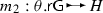 ,
,\({\textsf {acInc} } (H) \circ c_2=m_2\circ {\theta }{.}{{\textsf {ext} }} \),(items (9)+(10))
-
\(m_2\models _{\mathsf {BGC}} {\theta }{.}{{\textsf {rC} }} \),
-
-
(2)
-
 ,
, ,
, ,
, -
 is obtained by using the universal property of the coproduct \({\amalg } ({\theta }{.}{{\textsf {lX} }},{\theta }{.}{{\textsf {rX} }}) \),
 -
\(\gamma = k_1({G}{.}{{\textsf {ac} }})\wedge k_2({H}{.}{{\textsf {ac} }}) \rightarrow \sigma _{ VX }({\theta }{.}{{\textsf {ac} }}) \) is an AC, and
-
\({\textsf {sat} }_{\forall } (\gamma ) \),
-
 ,
, ,
, ,
, ,
, ,
, ,
, ,
, ,
, ,
, ,
, ,
, ,
, ,
, ,
, is obtained by using the universal property of the coproduct
 then  is an admissible comatch for the graph transformation span \(({\textsf {acInc} } (G) \circ b_1,{\textsf {acInc} } (H) \circ b_2)\), the match morphism \(m_1\), and the evolution pattern \(\theta \), written \(m_2\,\,{\in }\,\,{\textsf {admissible-comatches}}\,\, {(({\textsf {acInc} } (G) \,\,{\circ }\,\,b_1,\, {\textsf {acInc} } (H)}\,{\circ } b_2), {m_1},{\theta })\).

Visualization for Definition 30 (graph part)

Visualization for Definition 30 (AC part)
Note that, using the DPB approach mentioned above, we could alternatively construct  such that \(({\theta }{.}{{\textsf {del} }},d)\) is a pullback of \((c_1,b_1)\) and by constructing
  such that \(({\theta }{.}{{\textsf {add} }},d)\) is a pullback of \((c_2,b_2)\). A similar correspondence between DPO and DPB graph transformation has been presented e.g. in [48] where additional deletions are applied before the pushout complement is constructed. However, we believe that the definition above (albeit being more verbose) explains the construction of d and \(c_2\) more clearly by relying on the standard constructions for pushout complements and pushouts (the alternative DPB-based formalization requires the construction of pullback complements and pullbacks for the special case when three of the four morphisms are given already) and by presenting the additional deletions and additions using the two triangles explicitly.
We use this definition of admissible cospans below to propagate a match over the spans of a finite graph sequence for a given evolution pattern and a match of the left-hand side graph of the evolution pattern into the first graph of the given sequence. For this purpose, we now define the derived span of a graph sequence using the iterated pullback construction (cf. [31, Definition 4.1, p. 44]). This construction allows to contract a given finite graph sequence into a graph sequence of length one by forgetting about all interior steps of the sequence but preserving the relationship between elements of the first and the last graph of that sequence.Footnote 33 See Fig. 24 and Fig. 25a for a general visualization and an exemplary computation of a derived span.
Definition 31
(Derived Spans) If \(\pi \in \Pi ^{\mathsf {fin}}_{G_0,H} \) is a finite graph sequence that starts in \(G_0\) and that ends in H, then  , if one of the following items applies.
-
\({\textsf {length} }(\pi ) =0\) and \((\ell ,r)=({\textsf {id} } (G_0),{\textsf {id} } (G_0))\).
-
\({\textsf {length} }(\pi ) =1\) and \((\ell ,r)=\pi (0)\).
-
\({\textsf {length} }(\pi ) =2\), \(\pi (0)=(\ell _0,r_0)\), \(\pi (1)=(\ell _1,r_1)\), \((r_0',\ell _1')~\text {is a pullback of}~(r_0,\ell _1) \), and \((\ell ,r)=(\ell _0\circ r_0',r_1\circ \ell _1')\).
-
\({\textsf {length} }(\pi ) >2\) and \((\ell ,r)= {\textsf {derivedSpan} }(\{(0,{\textsf {derivedSpan} }(\{(0,\pi (0)),(1,\pi (1))\})), (1,{\textsf {derivedSpan} }(\{(n,x)\mid (n+2,x)\in \pi \}))\})\).

Visualization for Definition 31

A computation of a derived span from a graph sequence and the propagation of a match across the derived span. a We compute the derived span \((\ell _0\circ r_0',r_1\circ \ell _1')\) of a graph sequence of length 2. The construction of the pullback object X ensures that additional details about the interior graph \(G_1\) are lost. In particular, the temporary existence of the nodes c and \(a'\) (including their attributes and variables) together with the AC of \(G_1\) are lost. The returned derived span only contains information on the preservation of the node a (with its attribute and variable) across the graph sequence. b The derived span (bottom) from a (here given by \(({\textsf {acInc} } (G_0) \circ b_1,{\textsf {acInc} } (G_2) \circ b_2)=(\ell _0\circ r_0',r_1\circ \ell _1')\)) results in an admissible comatch using the operation admissible-comatches (we omit some of the details related to the graph part of the constructed diagram here for brevity) because the ACs of the graphs \(G_0\) and \(G_2\) imply the AC of the graph in the rule (top). That is, \(\wedge \{x_0= 0,x_1= 1,x'_0= 4,x'_2= 6,x'_4= 4 \} \) implies \(\wedge \{0\le x_0,x_0+4\le x_0',x_4'= x_0' \} \) as required where \(m_1\) maps \(y_0\) to \(x_0\) and \(m_2\) maps \(y_0'\) to \(x_0'\) and \(y_1'\) to \(x_4'\)
We now define the propagation of a match over a finite graph sequence for a given evolution pattern by obtaining the admissible comatches for the derived span computed for the given graph sequence. See Fig. 25b for an example of a match propagation over the derived span from Fig. 25a.
Definition 32
(Propagated Matches) If
-
\(\pi \in \Pi ^{\mathsf {fin}}_{G_0,H} \) is a finite graph sequence that starts in \(G_0\) and that ends in H,
-
\({\textsf {derivedSpan} }(\pi ) =(\ell ,r)\) is the derived span of \(\pi \),
-
\(\theta \in \mathcal {S}^{\mathsf {EP}} \) is an evolution pattern,
-
 is a match of the left-hand side graph of the evolution pattern \(\theta \) into the starting graph \(G_0\) of \(\pi \),
 -
 is a match of the right-hand side graph of the evolution pattern \(\theta \) into the ending graph H of \(\pi \), and
 -
\(m_2\in {\textsf {admissible-comatches}}{((\ell ,r)},{m_1},{\theta })\),
 is a match of the left-hand side graph of the evolution pattern
  is a match of the right-hand side graph of the evolution pattern
 then \(m_2\) is a match resulting from propagating the match \(m_1\) over \(\pi \) w.r.t. \(\theta \), written \(m_2\in {\textsf {PM} } (\pi ,m_1,\theta ) \).
Note that the definition of a propagated match can be used also in the reverse direction by reversing the rule and the graph sequence beforehand.
We now extend the propagation of matches to the case where a match is to be propagated over a subsequence of a TGS identified by two total timepoints. That is, given a TGS \(\pi \) that contains the TGS \(\pi '\) between two provided timepoints \(t_1\) and \(t_2\) where \(\pi '\) starts with graph G and ends with graph H, we want to propagate a match of L into G over the timed spans of \(\pi '\) into a match of a graph R into H. Reusing the match propagation defined above based on evolution patterns, this propagation may result in an empty set of matches when matched elements are deleted by the timed spans between \(t_1\) and \(t_2\). This time-based propagation operation is crucial for MTGL where we want to check e.g. whether a matched element also existed earlier (for the case when \(t_2<t_1\)) or exists later (for the case of \(t_2>t_1\)) in the given TGS \(\pi \). For the semantics of MTGL later on, we not only check for the existence of a suitable propagated match but also obtain the resulting matches of R into the graph in \(\pi \) at timepoint \(t_2\) to evaluate further conditions based on these resulting matches.
Definition 33
(Time-Based Propagated Matches) If
-
\(\pi \) and \(\pi '\) are TGSs from \(\Pi ^{ time }_{G_0} \),
-
\(\theta \in \mathcal {S}^{\mathsf {EP}} \) is an evolution pattern,
-
\({\theta }{.}{{\textsf {lG} }} =L\),
-
\({\theta }{.}{{\textsf {rG} }} =R\),
-
\(t_1\) and \(t_2\) are total timepoints from
 ,
, -
if \(t_1\le t_2\), then \(\pi '=\pi ^{\mathsf {T}}(\{t_1,t_2\}) \),
-
if \(t_1>t_2\), then \(\pi '={\textsf {rev} }(\pi ^{\mathsf {T}}(\{t_1, t_2\})) \),
-
 ,
, -
 are monomorphisms, and
 -
\(m_2\in {\textsf {PM} } (\pi ',m_1,\theta ) \) is a propagated match,
 ,
, ,
, are monomorphisms, and
then \(m_2\) is a time-based propagated match for \(m_1\) from \(t_1\) to \(t_2\) in \(\pi \) w.r.t. \(\theta \), written \(m_2\in {\textsf {PM} } (\pi ,t_1,t_2,m_1,\theta ) \).
Consider again Fig. 25a where the partial function \( time \) extracts the current time from the \(\text {id} \) attribute of node a. Then, Fig. 25b provides an example of a time-based propagation of the match \(m_1\) to the match \(m_2\) from the timepoint \(t_1=0\) (for the graph \(G_0\)) to the timepoint \(t_2=4\) (for the graph \(G_2\)).
7.2 Syntax and semantics of MTGL
We introduce the metric temporal graph logic (MTGL) with its syntax and semantics after a brief introduction of design choices.
Propositional temporal logics such as the linear temporal logic (LTL) can be defined on the foundation of labeled transition systems (S, R, L) containing a set of states S, a binary step relation \(R\subseteq S\times S\), and a labeling function  assigning a set of atomic propositions to each state. The conditions of such temporal logics then express properties that are to be satisfied by a given path of that labeled transition system. In particular, LTL allows to express (a) state properties based on elements of \( AP \) and propositional operators such as negation and conjunction as well as temporal operators to express (b) sequence properties based on the next operator stating that an LTL condition is satisfied in the next state and the until operator stating that an LTL property \(\phi _2\) is satisfied at some later state in the given path and that all states visited in between satisfy another LTL property \(\phi _1\). Further operators such as eventually and globally can be derived from the given operators.
Other temporal logics feature (a) operators that refer to earlier states using the operators previous and since (corresponding to the next and until operators), (b) metric temporal operators such as the metric-until operator that are then equipped with an interval describing the relative time at which the condition \(\phi _2\) has to be satisfied in the future,Footnote 34 and (c) combinations of (a) and (b) such as in the metric temporal logic (MTL) [60].
The use of atomic propositions in propositional temporal logics limits their expressiveness on the one hand but allows in some cases for the development of model checking approaches on the other hand [8]. In contrast, nonpropositional temporal logics do not make use of atomic propositions and may be defined on the more general Kripke frames where the labeling function of labeled transition systems is omitted. The goal of these logics is to express properties that cannot be expressed in propositional (metric) (temporal) logics. Such additional properties then refer to the content of states, which are given in our context by graphs in a TGS. For example, a particular element of such a graph may be tracked across multiple states. Other examples of nonpropositional (metric) temporal logics have been discussed e.g. in [9] (\(\mu \mathcal {G}2\): a combination of the \(\mu \)-calculus and second-order graph logic for labeled graphs) and [13] (metric temporal first-order logic (MFOTL): a combination of first-order logic using relations to store information and MTL).
We now introduce MTGL as a nonpropositional metric temporal logic where graphs are handled as first-class citizens meaning that conditions of MTGL directly contain graphs and graph morphisms as in BGL and GL instead of using encodings as in \(\mu \mathcal {G}2\) and MFOTL.
MTGL supports the two metric temporal operators \({\textsf {U} } \) (called until) and \({\textsf {S} } \) (called since) mentioned above. These two operators are, however, derived operators in our logic because we cover both of them using the operator  (called delta-lock). That is, delta-lock can be parameterized to behave like until or since. The nonpropositional character of MTGL is given by the use of matches of graphs from conditions of MTGL into the graphs of the TGS at hand. These matches are then propagated (as introduced in the previous subsection) over spans of the TGS allowing to express (using evolution patterns) conditions on how matched parts change over time. In particular, matches into graphs of the TGS are propagated forwards/backwards in the TGS for the until /since operator.
Moreover, MTGL supports the operator \(\boxdot \) (called delta-release), which is used in combination with delta-lock. For example, the special case of the until operator requires a propagation of a match m into a graph G of the TGS forwards resulting in a match \(m'\) but this forwards propagation alone only transfers information forwards. With delta-release, we allow to express statements that result in an additional backward propagation of \(m'\) into a match \(m''\) into the original graph G. The additional propagation of match \(m'\) allows to express statements at graph G based on graph elements and attributes matched by \(m'\).
Compared to [38, 81], we now additionally support conditions referring to the past but also handle the central capabilities of MTGL (binding of graph elements and comparison of attribute values) at a more fundamental level using evolution patterns and the delta-release operator, which leads to an increased expressiveness.
In MTGL, we specify sets of timepoints using ACs in the form of duration specifications, which have a single free variable \(\tau \in \mathcal {X} \) of sort \(\mathsf {real} \). The semantics of a duration specification \(\gamma \) is given by the set of all reals that satisfy \(\gamma \). For example, the interval \(I=[2,4)\) can be represented using \(\gamma =(2\le \tau )\wedge (\tau < 4) \) for which \({\textsf {sem} }(\gamma ) =I\). Moreover, for shifting of a duration specification, we formalize the statement \(\bar{x}\in {\textsf {sem} }(\gamma ) +\bar{y}\) where \(\bar{x}\) and \(\bar{y}\) are reals from \(\mathbf {R} \) using ACs. For this purpose, we represent \(\bar{x}\) and \(\bar{y}\) by variables x and y of sort \(\mathsf {real} \) and define an AC on these two variables. The resulting AC \(\gamma '\) then restricts x and y analogously to the statement \(\bar{x}\in {\textsf {sem} }(\gamma ) +\bar{y}\) above. For example, \(\bar{x}\in [2,4)+\bar{y}\) is represented using the AC \(\gamma =\exists \tau .\;x=\tau + y \wedge (2\le \tau )\wedge (\tau < 4) \).
Definition 34
(Duration Specification) If \(\tau \in \mathcal {X} \) is a variable, \({\textsf {sort} }_{} (\tau ) =\mathsf {real} \), and \(\gamma \in \mathcal {S}^{{\textsf {AC} }} _{\{\tau \}} \) is an AC that has only \(\tau \) as a free variable, then \(\gamma \) is a duration specification, written \(\gamma \in \mathcal {S}^{{\textsf {AC} }} _{{\textsf {DS} }(\tau )} \) or \(\gamma \in \mathcal {S}^{{\textsf {AC} }} _{{\textsf {DS} }} \).
Moreover, we define the following abbreviations.
-
induced semantics:
\({\textsf {sem} }(\gamma ) =\{x\in \mathbf {R} \mid \{\tau \mapsto x\}\models _{\mathsf {AC}} \gamma \}\) where \(\{\tau \mapsto x\}\) denotes the variable valuation that maps \(\tau \) to x.
-
shifting of a duration specification:
If x and y are variables from \(\mathcal {X} \),
then \({\textsf {shift} }_{\textsf {DS} } (\gamma ,x,y) =( \exists \tau .\;x=\tau + y \wedge \gamma )\in \mathcal {S}^{{\textsf {AC} }} _{\{x,y\}} \).
Note that many other metric temporal logics already impose the restriction that sets of timepoints must be specified by means of certain kinds of intervals. These logics thereby describe already on the syntax-level restrictions under which model checking of their conditions is decidable (see [19] for a survey on the expressiveness and algorithmic results for several metric temporal logics).
In the following, we introduce the metric temporal graph conditions (MTGCs) on a more detailed level. Firstly, MTGL supports the two propositional operators \(conjunction \) and \(negation \) as for GL and BGL and, secondly, the two metric temporal operators  (called \(delta{\text {-}}{}lock \)) and \(\boxdot \) (called \(delta{\text {-}}{}release \)). The \(delta{\text {-}}{}lock \) operator
  is an extension of the \(delta \) operator of GL. In addition to its right-hand side argument \((\theta _2,\psi _2)\) it has a left-hand side argument \((\theta _1,\psi _1)\) and a duration specification \(\gamma \) describing a delay \(\delta \in {\textsf {sem} }(\gamma ) \) as usual. For the special cases of the until and since operators, \((\theta _2,\psi _2)\) is checked at timepoint \(t+\delta \) and \((\theta _1,\psi _1)\) is checked for the timepoints between t and \(t+\delta \) (where \(\delta \ge 0\) corresponds to the case of until and \(\delta \le 0\) corresponds to the case of since). Moreover, the search restriction specifier \(\kappa \) is employed to further restrict the timepoints and matches used for satisfying \((\theta _2,\psi _2)\). In particular (see Fig. 26 for an example illustrating the differences between the search restriction specifiers), (a) \(\kappa =\mathsf {E} \) (called exists-match) imposes no further restriction and permits that any match compatible with the duration specification is used (for the duration specification \(\tau =0\) local state properties are stated and the duration specification \(\top \) allows to match elements at any timepoint in the TGS), (b) \(\kappa =\mathsf {N} \) (called new-match) imposes the restriction that \((\theta _2,\psi _2)\) could not be satisfied at some earlier (later) timepoint compared to \(t+\delta \) for \(\delta \ge 0\) (\(\delta <0\)) using the same binding (this search restriction specifier is used in our running example to determine the earliest time at which a result is added to be able to compare this earliest time with the imposed deadline), and (c) \(\kappa =\mathsf {C} \) (called closest-match) imposes the restriction that \((\theta _2,\psi _2)\) could not be satisfied at some timepoint \(t+\delta '\) that is closer to t than \(t+\delta \) by any binding (this search restriction specifier is motivated by the use of the state prophecy and state history operators from [77] that are able to focus on the next/previous match).

A TGS and three MTGCs exemplifying the usage of the search restriction specifier \(\kappa \) in MTGCs. a A TGS of length 3 where two nodes of type :A are created in addition to the node \(a_1\) in the initial graph. Note that we use a global variable \(x_{ tp }\) for encoding the current global time in this TGS. b The MTGC \(\psi _1\), which is satisfied by the TGS given in a because of any of the three nodes of type \({\text {:A}}\). With the duration specification \(\tau \ge 1 \) none of the three nodes is excluded since each of them exists at e.g. global time 2. c The MTGC \(\psi _2\), which is satisfied by the TGS given in a because of the nodes \(a_2\) and \(a_3\). With the duration specification \(\tau \ge 1 \) only the node \(a_1\) is excluded but \(a_2\) can be matched at time 1 and did not exist before and \(a_3\) can be matched at time 2 and did not exist before. d The MTGC \(\psi _3\), which is satisfied by the TGS given in a because of the node \(a_2\). With the duration specification \(\tau \ge 1 \) only the node \(a_1\) is excluded. The two other nodes \(a_2\) and \(a_3\) could be matched but the matching of \(a_3\) is prevented by the search restriction specifier because \(a_2\) can be matched and is closer to the initial checking time 0
A limitation of the \(delta{\text {-}}{}lock \) operator is that the satisfaction checks required for this operator (i.e., the check of \((\theta _1,\psi _1)\) for all timepoints between t and \(t+\delta \) and the check of \((\theta _2,\psi _2)\) at timepoint \(t+\delta \)) are executed in isolation from each other. This means that desired commonalities between these satisfaction checks in terms of matched graph elements and values of matched attributes require additional techniques.
Firstly, as demonstrated by the following example, the current context graph H at timepoint t determines a common part to be used in all these satisfaction checks.

A TGS and two MTGCs for Example 3 and Example 4. a A TGS of length 3 where different nodes of type :B are used in the first two graphs. Note that we use a global variable \(x_{ tp }\) for encoding the current global time in this TGS. b The MTGC \(\psi _1\), which formalizes the property “At the current timepoint, there is a node \(c{\text {:C}}\) (lines 1–3) that will be connected to a node of type :A with an id attribute of 1 within at most 120 time units (line 5) and until then, there is always a node of type :B with an id attribute of 1 connected to the node c (line 4)” from Example 3. The MTGC \(\psi _1\) is given in simplified notation in c and is satisfied by the TGS given in a. c The MTGC \(\psi _1\) from b in simplified notation. d The MTGC \(\psi _2\), which formalizes the property “There is a node \(c{\text {:C}}\) that is connected to a node \(a{\text {:A}}\) with an id attribute within at most 120 time units (lines 1–3) and until then, there is always a node \(b{\text {:B}}\) with an id attribute equal to the id attribute of the node a and the node b is connected to the node c (line 4)” from Example 4. The MTGC \(\psi _2\) is given in simplified notation in e and is satisfied by the TGS given in a. e The MTGC \(\psi _2\) from d in simplified notation
Example 3
(Forward Perspective of Binding and Values) Consider the following property.
-
Property: At the current timepoint, there is a node \(c{\text {:C}}\) that will be connected to a node of type :A with an id attribute of 1 within at most 120 time units and until then, there is always a node of type :B with an id attribute of 1 connected to the node c.
This property is an example where the binding of the node \(c{\text {:C}}\) is preserved forwards from the initial timepoint \(t=0\) over the TGS and is used in all satisfaction checks.
Secondly, we demonstrate in the following example a problem for sharing certain bindings among satisfaction checks at different timepoints. This problem is resolved subsequently using the additional MTGL operator delta-release. In the example, graph elements and values of attributes that are additionally matched at timepoint \(t+\delta \) by \((\theta _2,\psi _2)\) are not available when checking \((\theta _1,\psi _1)\) at the timepoints between t and \(t+\delta \).
Example 4
(Backward Perspective of Binding and Values) Consider the following property.
-
Property: There is a node \(c{\text {:C}}\) that is connected to a node \(a{\text {:A}}\) with an id attribute within at most 120 time units and until then, there is always a node \(b{\text {:B}}\) with an id attribute equal to the id attribute of the node a and the node b is connected to the node c.
This property is an example where the binding of the node \(c{\text {:C}}\) and the value of the id attribute of the node \(a{\text {:A}}\) is preserved backwards from the timepoint \(t+\delta \) toward the initial timepoint \(t=0\) over the TGS and is used in all satisfaction checks.
To specify properties as in the latter example, we employ the \(delta{\text {-}}{}release \) operator \(\boxdot (\theta ,\psi ) \), which has no counterpart in logics such as MTL without binding capabilities. The operator \(delta{\text {-}}{}release \) is used to specify, similarly to the left-hand side argument \((\theta _1,\psi _1)\) of the \(delta{\text {-}}{}lock \) operator, a property \((\theta ,\psi )\) that has to be satisfied in the obtained interval between t and \(t+\delta \). While the left-hand side argument \((\theta _1,\psi _1)\) of the \(delta{\text {-}}{}lock \) operator is checked for the TGS in the interval from the current time point t to the timepoint \(t+\delta \), the argument of the \(delta{\text {-}}{}release \) operator is checked in the reverse direction starting with a context graph established at the timepoint \(t+\delta \).
The two cases of forward and backward usage of contexts, as in the two examples above, are now covered as follows. Firstly, the left-hand side condition of the \(delta{\text {-}}{}lock \) operator is required when the condition that is to be checked in the interval depends on the binding that is obtained at the timepoint t as in Example 3. Secondly, the \(delta{\text {-}}{}release \) operator is required when the condition that is to be checked in the interval depends on the binding that is used to satisfy the right-hand side condition at the timepoint \(t+\delta \) of the \(delta{\text {-}}{}lock \) operator as in Example 4.
We now introduce the syntax of MTGL by formally defining its MTGCs.
Definition 35
(Metric Temporal Graph Conditions (MTGCs)) If \(H\in \mathbf {Graphs} \) is a graph and \(n\in \mathbf {N} \), then \(\bar{\psi }\) is a metric temporal graph condition (MTGC) over H of depth n, written \(\bar{\psi }\in {\mathcal {S}}_{n, {H}}^{\mathsf {MTGC}}\), if one of the following items applies.
- \(\bullet \):
-
\(\bar{\psi }=\wedge S \) and \(S\mathrel {\subseteq _{\mathsf {fin}}} {\mathcal {S}}_{n, {H}}^{\mathsf {MTGC}}\).
- \(\bullet \):
-
\(\bar{\psi }=\lnot \psi \) and \(\psi \in {\mathcal {S}}_{n, {H}}^{\mathsf {MTGC}}\).
- \(\bullet \):
-
 ,
, - \(\bullet \):
-
\(\theta _1\in \mathcal {S}^{\mathsf {EP}} \) is an evolution pattern with the left-hand side graph \({\theta _1}{.}{{\textsf {lG} }} =H\) and the right-hand side graph \({\theta _1}{.}{{\textsf {rG} }} =H_1'\),
- \(\bullet \):
-
\(\psi _1\in {\mathcal {S}}_{n, {H_1'}}^{\mathsf {MTGC}}\) is an MTGC over \(H_1'\) of the same depth n,
- \(\bullet \):
-
\(\gamma \in \mathcal {S}^{{\textsf {AC} }} _{{\textsf {DS} }} \) is a duration specification,
- \(\bullet \):
-
\(\kappa \in \{\mathsf {E},\mathsf {N},\mathsf {C} \}\) is a search restriction specifier,
- \(\bullet \):
-
\(\theta _2\in \mathcal {S}^{\mathsf {EP}} \) is an evolution pattern with the left-hand side graph \({\theta _2}{.}{{\textsf {lG} }} =H\) and the right-hand side graph \({\theta _2}{.}{{\textsf {rG} }} =H_2'\), and
- \(\bullet \):
-
\(\psi _2\in {\mathcal {S}}_{n+1, {H_2'}}^{\mathsf {MTGC}}\) is an MTGC over \(H_2'\) with increased depth \(n+1\).
- \(\bullet \):
-
\(\bar{\psi }=\boxdot (\theta ,\psi ) \),
- \(\bullet \):
-
\(n>0\) indicates at least one enclosing delta-lock operator to which \(\bar{\psi }\) refers to,
- \(\bullet \):
-
\(\theta \in \mathcal {S}^{\mathsf {EP}} \) is an evolution pattern with the left-hand side graph \({\theta }{.}{{\textsf {lG} }} =H\) and the right-hand side graph \({\theta }{.}{{\textsf {rG} }} =H'\), and
- \(\bullet \):
-
\(\psi \in {\mathcal {S}}_{n-1, {H'}}^{\mathsf {MTGC}}\) is an MTGC over \(H'\) with decreased depth \(n-1\).
 ,
, Moreover, we define the following abbreviations.
-
\({\mathcal {S}}_{H}^{\mathsf {MTGC}}={\mathcal {S}}_{0, H}^{\mathsf {MTGC}}\) contains the MTGCs of depth 0.
-
true: \(\top =\wedge \varnothing \).
-
false: \(\bot =\lnot \top \).
-
disjunction: \(\vee S =\lnot (\wedge \{\lnot \psi \mid \psi \in S\}) \).
Note that in the definition above, we only permit occurrences of the \(delta{\text {-}}{}release \) operator in the right-hand side argument of the \(delta{\text {-}}{}lock \) operator. Moreover, we use a depth parameter \(n\in \mathbf {N} \) for the number of open \(delta{\text {-}}{}lock \) calls to ensure that the number of \(delta{\text {-}}{}release \) calls does not exceed the number of \(delta{\text {-}}{}lock \) calls (i.e., to ensure that each instance of the \(delta{\text {-}}{}release \) operator has an enclosing instance of the \(delta{\text {-}}{}lock \) operator). The use of this depth parameter guarantees in the semantics of MTGL (as explained in more detail below) that whenever an instance of the \(delta{\text {-}}{}release \) operator is checked, a timepoint specifying the origin of a previous instance of the \(delta{\text {-}}{}lock \) operator is available.
The formalization of the properties from Example 3 and Example 4 is given in Fig. 27b and Fig. 27d, respectively, where we use the notation introduced subsequently.
Notation 5
(Evolution Patterns in MTGCs) We adapt our notation for GCs from Notation 3 as follows. For the delta-lock and delta-release operators, we depict the evolution patterns in five compartments separated by vertical lines assuming that \({\theta }{.}{{\textsf {res} }} \), \({\theta }{.}{{\textsf {del} }} \), \({\theta }{.}{{\textsf {add} }} \), and \({\theta }{.}{{\textsf {ext} }} \) are inclusion morphisms. We depict the morphisms \({\theta }{.}{{\textsf {res} }} \) and \({\theta }{.}{{\textsf {del} }} \), by employing the notation for monomorphisms used in a restrict operator, in the first and second compartment, respectively. We depict the morphisms \({\theta }{.}{{\textsf {add} }} \) and \({\theta }{.}{{\textsf {ext} }} \), by employing the notation for monomorphisms used in an exists operator, in the third and fourth compartment, respectively. Lastly, we depict \({\theta }{.}{{\textsf {ac} }}\) in the firth compartment. If one of the monomorphisms is an identity morphism, we denote this by \({\textsf {id} } \). If \({\theta }{.}{{\textsf {res} }} \) or \({\theta }{.}{{\textsf {del} }} \) is an initial morphism from the empty graph, we denote this by \(\varvec{\varnothing } \). If one of the monomorphisms is not an inclusion morphism or one of the application conditions \({\theta }{.}{{\textsf {lC} }}\) or \({\theta }{.}{{\textsf {rC} }}\) is not \(\top \), we use our more general notation for evolution patterns from Notation 4.

Formalization of the three metric temporal properties from Example 1 as MTGCs. a The MTGC \(\psi _1\), which formalizes the property “Each task that is spawned in a system is eventually completed and thereby removed from the system within at most 10000 time units and produces a unique result with a value of \( ok \) and an id that equals the id of the task.” b The MTGC \(\psi _2\), which formalizes the property “Each new result is obtained from a task with the same id that was spawned at most 10000 time units before and that was present since then.” c The MTGC \(\psi _3\), which formalizes the property “Every task in a system runs at least once every 1000 time units until it terminates”
Since some of the arguments of the delta-lock and delta-release operators are trivial in concrete MTGCs, we provide abbreviations for such cases in Table 1 introducing further derived operators leading to a simplified notation for MTGCs as used in Fig. 27c and Fig. 27e. That is, these additional derived operators should increase applicability of our logic by allowing for more concise MTGCs and by using more intuitive operators such as since and until. Note that the argument \((\varvec{\varnothing } \mid {\textsf {id} } \mid {\textsf {id} } \mid {\textsf {id} } \mid \top ,\top )\), which is used in some left-hand sides of delta-lock operators in the table, does not impose any limitations to be checked for satisfaction. Hence, this argument can be understood to be neutral because it restricts the match to the empty graph, does not require deletions, does not require additions, does not require additional matchings, does not impose restrictions using the trivial AC \(\top \), and the MTGC \(\top \) does not require further properties to be satisfied.
-
restrict:

Restriction of the current match according to the monomorphism f. Note that there is no dual operator because the restriction is unique. Moreover, we only permit the search restriction specifier \(\kappa =\mathsf {E} \) for this operator because the restriction is always possible.
-
deletion:
Deletion of matched graph elements according to the monomorphism f. Note that there is no dual operator because the deletion is unique.
-
exists-addition:

Addition and matching of further graph elements according to the monomorphism f.
-
forall-addition:

The operator that is dual to the exists-addition operator considering all additions.
-
exists:

Extension of the current match according to the monomorphism f.
-
forall:

The operator that is dual to the exists operator considering all extensions.
-
until: \((\theta _1,\psi _1)\mathrel {{\textsf {U} } ^{\kappa }_{\gamma }}(\theta _2,\psi _2) \)
The standard until operator known from other metric temporal logics such as MTL. The operator requires in addition that the duration specification describes only positive delays \(\delta \).
-
eventually: \(\lozenge ^{\kappa }_{\gamma }(\theta ,\psi ) \)
The standard eventually operator known from other metric temporal logics such as MTL. It is a simple case of the until operator with a neutral left-hand side argument.
-
globally: \(\square ^{\kappa }_{\gamma }(\theta ,\psi ) \)
The operator that is dual to the eventually operator considering all future timepoints that are compatible with \(\gamma \).
-
since: \((\theta _1,\psi _1)\mathrel {{\textsf {S} } ^{\kappa }_{\gamma }}(\theta _2,\psi _2) \)
The standard since operator known from other metric temporal logics such as MTL. The operator requires in addition that the duration specification describes only negative delays \(\delta \).
-
once: \(\blacklozenge ^{\kappa }_{\gamma }(\theta ,\psi ) \)
Similar operator to eventually for the past. It is a simple case of the since operator with a neutral left-hand side argument.
-
historically: \(\blacksquare ^{\kappa }_{\gamma }(\theta ,\psi ) \)
Similar operator to globally for the past. The operator that is dual to the once operator considering all past timepoints that are compatible with \(\gamma \).
-
forall-matches: \(\kappa =\mathsf {A} \)
The additional search restriction specifier \(\mathsf {A} \) (called \(forall{\text {-}}{}matches \)) results in a dual operator compared to the search restriction specifier \(\mathsf {E} \).


Note that we permit that the search restriction specifier \(\kappa \) and the duration specification \(\gamma \) are omitted when \(\kappa =\mathsf {E} \) and \(\gamma =(\tau = 0)\), respectively. Based on the abbreviations from above, we provide the MTGCs from Fig. 27b and Fig. 27d in simplified notation in Fig. 27c and Fig. 27e, respectively. Also, for our running example, we provide in Fig. 28 a formalization of the properties \(\mathbf {P_{1}}\), \(\mathbf {P_{2}}\), and \(\mathbf {P_{3}}\) introduced in Example 1.
We now define the inductive satisfaction relation of MTGL for MTGCs and TGSs.
-
As a special case, the satisfaction relation is defined for an MTGC \(\bar{\psi }\) over the empty graph of depth 0, a TGS \(\pi \in \Pi ^{ time }_{G} \), the empty word \(\lambda \) of timepoints used for the delta-release operator, the initial checking time \( time (G) =0\), and the initial match \(m={\textsf {i} } (G) \) representing an empty binding.
-
For the general case, the satisfaction relation is defined for an MTGC \(\bar{\psi }\) over a graph H of depth n, a TGS \(\pi \in \Pi ^{ time }_{G} \), a word \( ts \) of n timepoints from
 , a current checking time
  , and a match
  representing the current binding. Hence, timepoints may not exceed the duration of the TGS in both cases.
 , a current checking time
  , and a match
  representing the current binding. Hence, timepoints may not exceed the duration of the TGS in both cases.
The depth n of \(\bar{\psi }\) must be equal to the length of \( ts \) to ensure that each occurring delta-release operator has a corresponding timepoint in \( ts \), which specifies the origin of a previous instance of the \(delta{\text {-}}{}lock \) operator. In the following definition of the satisfaction relation, we heavily rely on the operation \({\textsf {PM} } \) for time-based propagation of matches from Definition 33 to change the target of the current match m from \(\pi ^{\mathsf {T}}(t) \) to graphs at later/earlier timepoints \(\pi ^{\mathsf {T}}(t+\delta ) \). In particular, \({\textsf {PM} } (\pi ,t,t+\delta ,m,\theta ) \) comprises the matches obtained from propagating the match m from timepoint t to timepoint \(t+\delta \) in \(\pi \) w.r.t. \(\theta \). Recall that this set can have zero, one, or more elements in general.
The satisfaction relation of MTGL is defined as the satisfaction relation of GL for the operators conjunction and negation and also covers the two additional operators delta-lock and delta-release.
Definition 36
(Satisfaction of MTGCs) If \(\pi \in \Pi ^{ time }_{G} \) is a TGS,  is a word of n timepoints,
  is a timepoint,
  is a partially injective monomorphism, and \(\bar{\psi }\in {\mathcal {S}}_{n ,H}^{\mathsf {MTGC}}\) is an MTGC over H of depth n, then \((\pi , ts ,t,m)\models _{\text {MTGC}} \bar{\psi } \), if one of the following items applies.
- \(\bullet \):
-
\(\bar{\psi }=\wedge S \) and \(\forall \psi \in S.\;(\pi , ts ,t,m)\models _{\text {MTGC}} \psi \).
- \(\bullet \):
-
\(\bar{\psi }=\lnot \psi \) and \((\pi , ts ,t,m)\not \models _{\text {MTGC}} \psi \).
- \(\bullet \):
-
 and there are \(\delta \in {\textsf {sem} }(\gamma ) \) andFootnote 35\(\tilde{m}\in {\textsf {PM} } (\pi ,t,t+\delta ,m,\theta _2) \) s.t.
 - \(\bullet \):
-
\((\pi , ts \cdot t,t+\delta ,\tilde{m})\models _{\text {MTGC}} \psi _2 \),Footnote 36
- \(\bullet \):
-
if \(\kappa =\mathsf {N} \),
I is an intervalFootnote 37 over
 ,
,\(I=[0,t+\delta )\) if \(\delta \ge 0\),
and \(I=(t+\delta ,\infty )\) if \(\delta <0\),
then each

satisfies \({\textsf {PM} } (\pi ,t+\delta ,t',\tilde{m},{\textsf {id} }) =\varnothing \),Footnote 38
- \(\bullet \):
-
if \(\kappa =\mathsf {C} \),
then each \(\delta '\in ((\delta ,0]\cup [0,\delta ))\cap {\textsf {sem} }(\gamma ) \)
satisfies \({\textsf {PM} } (\pi ,t,t+\delta ',m,\theta _2) =\varnothing \),Footnote 39 and
- \(\bullet \):
-
for each \(\delta '\in (\delta ,0]\cup [0,\delta )\)
there is \(\tilde{m}\in {\textsf {PM} } (\pi ,t,t+\delta ',m,\theta _1) \)
s.t. \((\pi , ts ,t+\delta ',\tilde{m})\models _{\text {MTGC}} \psi _1 \).Footnote 40
- \(\bullet \):
-
\(\bar{\psi }=\boxdot (\theta ,\psi ) \), \( ts = ts' \cdot t'\), and
for each \(t''\in [t',t)\cup (t,t']\)
there is \(\tilde{m}\in {\textsf {PM} } (\pi ,t,t'',m,\theta ) \)
s.t. \((\pi , ts ',t'',\tilde{m})\models _{\text {MTGC}} \psi \).Footnote 41
 and there are
  ,
,
Also, if \(\bar{\psi }\in {\mathcal {S}}_{\varvec{\varnothing }}^{\mathsf {MTGC}}\) and \((\pi ,\lambda ,0,{\textsf {i} } (G))\models _{\text {MTGC}} \bar{\psi } \), then \(\pi \models _{\text {MTGC}} \bar{\psi } \).

An example of a TGS and an MTGC for comparing point-based and interval-based semantics. a The TGS \(\pi \), which is parameterized with a duration \(\delta \ge 0\). b The MTGC \(\psi \), which formalizes the property “In at most 4 time units there is some node \(a{\text {:A}}\) such that in at most 4 time units there is some node of type :B connected to a”
For our running example, see Fig. 15 for a TGS \(\pi \), which does not satisfy the MTGC \(\psi _1\) from Fig. 28a. The TGS \(\pi \) does not satisfy \(\psi _1\) because, for the node \(T_2\) of type :Task created at the timepoint 102 with \(\text {id}\) attribute 1, there is not eventually a unique node R of type \({\text {:Result}}\) with \(\text {id}\) attribute 1 and \(\text {value} \) attribute \( ok \). Indeed, the node \(R_2\) is the only node of type \({\text {:Result}}\) that is created in the described timepoint interval with the \(\text {id}\) attribute 1 of the node \(T_2\) and \(\text {value} \) attribute \( ok \) but there is the additional node \(R_1\) of type \({\text {:Result}}\) with the \(\text {id}\) attribute 1, which invalidates uniqueness. Basically, the absence of such nodes of type \({\text {:Result}}\) generated from previous tasks is not ensured using an application condition in the rule \(\rho _{ SpawnTask }\) in Fig. 13a. The error occurs when an old result is not yet removed using the rule \(\rho _{ ConsumeResult }\) and is more likely in real systems when the set of admissible \(\text {id}\) attributes is smallFootnote 42 or when they are chosen in a deterministic order.
Metric temporal logics vary not only in their selection of operators (such as until and since) and the underlying data structures for states (such as graphs, relations, and sets of atomic proposition) but also in their interpretation of how continuous time is related to discrete steps. In [75] two basic alternative kinds of semantics are discussed. On the one hand, point-based semantics such as in MFOTL [13] (also see [4, 5, 51, 53, 54, 84]) quantify for the metric temporal operators over the countable set of timepoints in a dense-time interval that are associated to the events that alter the state, which means that, effectively, only discrete steps are considered that are associated with a continuous variable representing the current global time. On the other hand, interval-based semantics such as in MTGL (also see [3, 6, 52, 77]) quantify for the metric temporal operators over all timepoints in the entire dense-time interval. As argued in [75], a common reason for using the point-based semantics is that MTL satisfiability is decidable for the point-based semantics but not for the interval-based semantics. However, while deciding MTGL satisfiability is generally also of interest to exclude unsatisfiable MTGC -based specifications, it is not our focus as of now.
By means of the example in Fig. 29, we now discuss the general difference between point-based and interval-based semantics. The TGS \(\pi \) from Fig. 29a satisfies the MTGC \(\psi \) from Fig. 29b when \(\delta \le 6\) because the node of type :A can be matched at global time 4, which permits to wait for the required node of type \({\text {:B}}\) for 4 further time units until global time 8. In comparison, when the corresponding TGS and the corresponding condition in MFOTL are considered, it turns out that \(\delta \le 4\) is required for satisfaction because the point-based semantics of MFOTL can only jump to the global time 2 for matching the node of type :A. Hence, as also mentioned in [75], point-based semantics takes the perspective of specifying events whereas interval-based semantics takes the perspective of specifying states.
7.3 Folding of timed graph sequences
We now introduce the operation \({\textsf {Fold} }^{\textsf {tgs} } \) for translating TGSs that contain only grounded graphs (where each variable has a unique value) into a single graph, which is called graph with history (GH). This GH contains for each node and edge occurring in the TGS the total timepoint when it was created and, if it was deleted, the total timepoint when it was deleted. To capture these total timepoints, we use additional \(\text {cts} \) (creation timestamp) and \(\text {dts} \) (deletion timestamp) attributes of sort \(\mathsf {real} \).Footnote 43 See Fig. 12a where we have added such attributes in the type graph already for our running example. Furthermore, for our running example, we obtain the GH in Fig. 15b from the TGS given in Fig. 15a. Note that, in comparison to the notion of a derived span (see Definition 31), which drops all interior information contained in a graph sequence or a TGS, we now want to collect all this interior information into the resulting GH.
Definition 37
(Graphs with History (GHs)) If
-
\( TG \) is a type graph where all nodes and edges have attributes \(\text {cts} \) and \(\text {dts} \) of sort \(\mathsf {real} \),
-
\(G_H\in \mathbf {Graphs} \) is a graph typed over \( TG \),
-
each node and edge in \(G_H\) has unique attributes \(\text {cts} =x\) and \(\text {dts} =y\) satisfying \(0\le x \) (since the global time is assumed to start at 0) and \(y=-1 \) or \(x< y \) (since graph elements are either not yet deleted or are deleted after they have been created),
-
for each edge e in \(G_H\), the value of the \(\text {cts} \) attributes of the source and the target nodes of e is less or equal than the \(\text {cts} \) attribute of e,
-
for each edge e in \(G_H\), the value of the \(\text {dts} \) attributes of the source and the target nodes of e is greater or equal than the \(\text {dts} \) attribute of e,
then \(G_H\) is a graph with history (GH).
To fold a finite TGS, we first obtain a GH from the first graph of a TGS.
Definition 38
(Operation \({\textsf {Fold} }^{\textsf {1st} }\)) If \(G\in \mathbf {Graphs} \) is a graph and  is an inclusion morphism obtained by
-
adding the attribute \(\text {cts} =0\) to all nodes in G,
-
adding the attribute \(\text {dts} =-1\) to all nodes in G,
-
adding the attribute \(\text {cts} =0\) to all edges in G, and
-
adding the attribute \(\text {dts} =-1\) to all edges in G,
then  is the graph-folding of the graph G into the GH \(G'\), written \({\textsf {Fold} }^{\textsf {1st} } (G) =m\).
Note that the inclusion morphism  identifies the elements of the graph G in its GH \(G'\).
We now define the operation that folds a single span  for a given monomorphism
  into a monomorphism
  where \(G'\) and \(H'\) are GHs of G and H, respectively. The resulting monomorphism \(m'\) is obtained as follows. For nodes and edges freshly added by r, we add \(\text {cts}\) attributes set to the current global time (extracted from H) and add \(\text {dts}\) attributes initially set to \(-1\) (denoting that these elements have not yet been deleted). Moreover, for nodes and edges freshly deleted by \(\ell \), we add \(\text {dts}\) attributes set to the current global time (extracted from H) and remove the \(\text {dts} =-1\) attributes previously included. Note that the following definition does not depend on the syntactic representation of the ACs of graphs (which we want to handle up to equivalence). Instead, we wrap ACs of graphs in additional quantification and conjunction and silently assume that such ACs of graphs are simplified as in our exemplary application in Fig. 15. See Fig. 30 for an accompanying visualization.
Definition 39
(Operation \({\textsf {Fold} }^{\textsf {span} }\)) If
-
 is a monomorphism,
 -
 is a span,
 -
\(N_2={m}{.}{{\textsf {N} }} ({G}{.}{{\textsf {N} }}-{\ell }{.}{{\textsf {N} }} ({D}{.}{{\textsf {N} }}))\) contains the nodes that are removed by \(\ell \),
-
\(E_2={m}{.}{{\textsf {E} }} ({G}{.}{{\textsf {E} }}-{\ell }{.}{{\textsf {E} }} ({D}{.}{{\textsf {E} }}))\) contains the edges that are removed by \(\ell \),
-
\(D'\) is obtained from \(G'\) resulting in some monomorphism
 and an inclusion
  satisfying \(m\circ \ell =b_1\circ d\) by
 -
(1)
setting the set of variables V to be empty,
-
(2)
removing the \(\text {dts} =-1\) attributes from nodes and edges in \(N_2\) and \(E_2\) while adding the local variables that are connected to these attributes to V, and
-
(3)
setting \({D'}{.}{{\textsf {ac} }} \) to \(\exists V.\;{G'}{.}{{\textsf {ac} }} \) to adapt the AC according to the removal of the variables in V,
-
(1)
-
 that adds the elements freshly added by r to \(D'\) resulting in the graph X,
 -
\( time (H) =t\) is the current global time of H,
-
\(N_1={\bar{m}}{.}{{\textsf {N} }} ({H}{.}{{\textsf {N} }}-{r}{.}{{\textsf {N} }} ({D}{.}{{\textsf {N} }}))\) contains the nodes that are added by r,
-
\(E_1={\bar{m}}{.}{{\textsf {E} }} ({H}{.}{{\textsf {E} }}-{r}{.}{{\textsf {E} }} ({D}{.}{{\textsf {E} }}))\) contains the edges that are added by r,
-
\(H'\) is obtained from X resulting in some monomorphisms
 and
and  satisfying \(m'=b_3\circ \bar{m}\) by
 -
(1)
setting the set of ACs S to be empty,
-
(2)
adding the attributes \(\text {cts} =t\) and \(\text {dts} =-1\) with fresh local variables to all nodes and edges in \(N_1\) and \(E_1\) while inserting the used ACs into S,
-
(3)
adding the attribute \(\text {dts} =t\) with a fresh local variable to all nodes and edges in \(b_2(N_2)\) and \(b_2(E_2)\) while inserting the used ACs into S, and
-
(4)
setting \({H'}{.}{{\textsf {ac} }} \) to some AC that is equivalent to \({X}{.}{{\textsf {ac} }} \wedge (\wedge S) \),
-
(1)
 is a monomorphism,
 is a span,
 and an inclusion
  satisfying
  that adds the elements freshly added by r to
  and
and  satisfying
 then  is the span-folding of the span \((\ell ,r)\) w.r.t. the monomorphism
  into the GH \(H'\), written \({\textsf {Fold} }^{\textsf {span} } (m,(\ell ,r)) =m'\).

Visualization for Definition 39
Finally, we define the iterated folding of an entire finite TGS using the operations \({\textsf {Fold} }^{\textsf {1st} }\) and \({\textsf {Fold} }^{\textsf {span} }\).
Definition 40
(Operation \({\textsf {Fold} }^{\textsf {tgs} }\)) If \(\pi \in \Pi ^{\mathsf {fin}, time }_{G,H} \) is a finite TGS starting in G and ending in H, and  ,
,  are monomorphisms, then \(m'\) is the tgs-folding of \(\pi \) w.r.t. the monomorphism m, written \({\textsf {Fold} }^{\textsf {tgs} } (m,\pi ) =m'\), if one of the following items applies.
-
\({\textsf {length} }(\pi ) =0\) and \(m'=m\).
-
\({\textsf {length} }(\pi ) >0\) and \(m'={\textsf {Fold} }^{\textsf {tgs} } ({\textsf {Fold} }^{\textsf {span} } (m,\pi (0)), \{(k,x)\mid (k+1,x)\in \pi \})\).
Also, if \({\textsf {Fold} }^{\textsf {tgs} } ({\textsf {Fold} }^{\textsf {1st} } (G),\pi ) =m'\), then \(m'\) is the tgs-folding of \(\pi \), written \({\textsf {Fold} }^{\textsf {tgs} } (\pi ) =m'\).
Since the operation \({\textsf {Fold} }^{\textsf {span} }\) above also constructs a span  from the GH \(G'\) to the GH \(H'\), we can observe that the incremental folding executed by \({\textsf {Fold} }^{\textsf {tgs} } \) straightforwardly results in the construction of a TGS \(\pi '\) of GHs where the ith GH in \(\pi '\) corresponds to the folding of the prefix of \(\pi \) of length i.
See Fig. 15b for an example of a GH that is obtained from the TGS given in Fig. 15a using \({\textsf {Fold} }^{\textsf {tgs} }\).
It is important to point out that timepoints of attribute modifications are not directly recorded in the GH by the folding operations introduced here. As a consequence, attributes that are referred to by MTGCs and that may be changed in a given TGS often need to be contained in separate nodes to be able to track their values over time when using our encoding-based approach presented in the next subsection. The reason for this is that deleted node and edge attributes remain in the GH and that only the last value of an attribute is stored in the GH. This is particularly helpful for the current global time that may be recorded in an attribute that is matched and preserved in each step (cf. our running example where the \(\text {time} \) attribute of the system node is changed when applying a rule from Fig. 13 or Fig. 14). In our running example, we change the attribute \(\text {limit} \) of systems when spawning new tasks but we do not refer to this attribute in the MTGCs in Fig. 26. However, we change the attribute \(\text {dur} \) of tasks and refer to this attribute in the MTGC \(\psi _3\) in Fig. 26d. Hence, in our tool-based evaluation, we use the adapted type graph from Fig. 31 where the attribute \(\text {dur} \) of a task is stored in an additional node for which \(\text {cts} \) and \(\text {dts} \) attributes are then added by the folding operations presented above. The adaption of a given type graph to store node and edge attribute is always possible but we omit its formal handling here since also the rules of the (timed) graph transformation system as well as the MTGCs would need to be adapted to such a changed type graph as well on a technical level.

The adapted type graph \( TG '\) containing an additional node storing the attribute \(\text {dur} \) for tasks

Encoding of the MTGC from Fig. 28a using 
7.4 Encoding of MTGL in GL
The problem of satisfaction checking for metric temporal logics is far more difficult than for temporal logics because the intervals during which elements are alive (i.e., during which atomic proposition are satisfied) must be checked w.r.t. the intervals provided in the condition. Moreover, this problem is especially difficult when operators such as until or since are nested. This observation is also true for the case for MTGL where a procedure for checking the satisfaction of a given MTGC by a TGS is difficult for nested delta-lock operators. To obtain an effective and suitably efficient procedure for MTGL satisfaction checking, we now continue by presenting an encoding in the form of the operation  , which translates MTGCs into GCs.Footnote 44 In the context of our general approach (cf. Fig. 1), we define
  such that it is compatible with the operation \({\textsf {Fold} }^{\textsf {tgs} }\) from Definition 40. To this end, we provide support for MTGL satisfaction checking via the two operations \({\textsf {Fold} }^{\textsf {tgs} }\) and
  that simplify the satisfaction checking problem to the setting of GL for which we can then employ tool support or apply the further encodings \({\textsf {enc} }_{\Delta }\) and \({\textsf {enc} }_{\nu }\) if desired. That is, instead of checking satisfaction for a given MTGC \(\psi \) and a given TGS \(\pi \), we check whether the GH obtained from \(\pi \) using \({\textsf {Fold} }^{\textsf {tgs} }\) satisfies the GC \(\phi \) obtained by applying
  to \(\psi \). For our running example, we have applied the operation \({\textsf {Fold} }^{\textsf {tgs} }\) to the TGS given in Fig. 15a to obtain the GH from Fig. 15b.
The operation  relies on the fact that the GH obtained from folding a TGS contains for each node/edge occurring in the TGS so far the timepoints of creation and (if it was deleted) deletion using additional \(\text {cts}\) and \(\text {dts}\) attributes. We subsequently refer to the variables that are connected to the \(\text {cts}\) and \(\text {dts}\) attributes of a node/edge \(\alpha \) using \(x_{c,\alpha }\) and \(x_{d,\alpha }\), respectively. For our running example, the type graph \( TG \) containing such \(\text {cts}\) and \(\text {dts}\) attributes is given in Fig. 12a.
The GC that is obtained using the operation  from an MTGC encodes the checks for MTGL operators according to the semantics of MTGL from Definition 36 using additional global variables for quantifying over observation timepoints. Moreover, additional ACs that refer to the \(\text {cts}\) and \(\text {dts}\) attributes are used to ensure that all additionally matched elements have been created and not yet deleted w.r.t. a timepoint or, alternatively, that elements that are no longer matched have been deleted before a timepoint when this is required.
We now introduce four minor operations used in the operation  later on.
The operation \({\textsf {alive} }\) returns for a graph H an AC. The graph H is part of the GC obtained below using  for a given MTGC and the AC obtained using \({\textsf {alive} }\) is then part of the AC of H. The purpose of the generated AC is that when the operation \({\textsf {Fold} }^{\textsf {tgs} }\) generates a GH for a given TGS \(\pi \), then H can only be matched to graph elements of that GH for a given global time represented by a variable x when each matched graph element exists in the graph of \(\pi \) at the global time stored in x. That is, the AC ensures that all of the matched nodes/edges have been created before the timepoint given by x and that none of them has been deleted before the timepoint given by x.
Definition 41
(Operation \({\textsf {alive} }\)) If H is a graph where \(x_{c,\alpha }\) and \(x_{d,\alpha }\) denote the local variables connected to the \(\text {cts}\) and \(\text {dts}\) attribute of a node/edge \(\alpha \in {H}{.}{{\textsf {N} }} \cup {H}{.}{{\textsf {E} }} \) of H and x is a global variable of sort \(\mathsf {real}\) contained in H, then \({{\textsf {alive} }(x,H)} = \wedge \{x_{c,\alpha }\le x \wedge (x_{d,\alpha }=-1 \vee x< x_{d,\alpha } ) \mid \alpha \in {H}{.}{{\textsf {N} }} \cup {H}{.}{{\textsf {E} }} \} \).
The operation \({\textsf {earliest} }\) is used in a similar way for a graph H and returns also an AC to be used in H. The difference is that the AC generated by \({\textsf {earliest} }\) ensures that none of the matched graph elements existed before the global time given by the variable x. That is, one of the matched graph elements called \(\alpha \) must have been created at the timepoint given by x and none of the other graph elements \(\beta \) must have been created after that timepoint. This AC thereby ensures that the graph H could not have been matched to the same elements at an earlier timepoint because the graph element \(\alpha \) could not have been matched earlier. The AC generated by \({\textsf {earliest} }\) in this way is used in  when encoding an MTGC using the search restriction specifier new-match.
Definition 42
(Operation \({\textsf {earliest} }\)) If H is a graph where \(x_{c,\alpha }\) and \(x_{d,\alpha }\) denote the local variables connected to the \(\text {cts}\) and \(\text {dts}\) attribute of a node/edge \(\alpha \in {H}{.}{{\textsf {N} }} \cup {H}{.}{{\textsf {E} }} \) of H and x is a global variable of sort \(\mathsf {real}\) contained in H, then \({{\textsf {earliest} }(x,H)} =\vee \{\wedge (\{x_{c,\alpha }=x\}\cup \{x\ge x_{c,\beta } \mid \beta \in S-\{\alpha \}\}) \mid \alpha \in {H}{.}{{\textsf {N} }} \cup {H}{.}{{\textsf {E} }} \} \).
For our running example, see Fig. 32 for the GC that results from applying the operation  , which is introduced in the following, to the MTGC from Fig. 28a where we make use of ACs including the operations \({\textsf {alive} }\) and \({\textsf {earliest} }\). Note that, to simplify notation, we also apply \({\textsf {alive} }\) and \({\textsf {earliest} }\) by just providing a set of graph elements instead of an entire graph.
The operation \({\textsf {ruleAdd} }\) creates a restriction-extension pattern by adding a set of global variables V, by adding a further global variable x, and by requiring the satisfaction of an AC \(\gamma \). Also, the restriction-extension pattern additionally subsumes a given context graph H and its AC states that the variables in V remain unchanged. Restriction-extension patterns constructed using \({\textsf {ruleAdd} }\) are used to quantify over the additional global variable x that represents an observation timepoint in the satisfaction relation of MTGL (see Definition 36).
Definition 43
(Operation \({\textsf {ruleAdd} }\) ) If
-
\(H\in \mathbf {Graphs} \) is a graph,
-
\(V\cup \{x\}\subseteq \mathcal {X} \) are variables,
-
\(\gamma \in \mathcal {S}^{{\textsf {AC} }} _{V\cup \{x\}\cup {H}{.}{{\textsf {X} }}} \) is an AC,
-
\(\bar{H}\) is derived from H by
setting \({\bar{H}}{.}{{\textsf {XG} }} ={H}{.}{{\textsf {XG} }} \cup V\),
-
\(\bar{H}'\) is derived from \(\bar{H}\) by
setting \({\bar{H}'}{.}{{\textsf {XG} }} ={\bar{H}}{.}{{\textsf {XG} }} \cup \{x\}\),
-
\(\rho \in \mathcal {S}^{\mathsf {REP}} \) is a restriction-extension pattern,
-
\({\rho }{.}{{\textsf {res} }} ={\textsf {id} } (\bar{H}) \),
-
\({\rho }{.}{{\textsf {ext} }} ={\textsf {inc} } (\bar{H},\bar{H}') \),
-
\({\rho }{.}{{\textsf {ac} }} =\wedge (\{\gamma \}\cup \{{\theta }{.}{{\textsf {lX} }} (y)= {\theta }{.}{{\textsf {rX} }} (y) \mid y\in V\}) \), and
-
\({\rho }{.}{{\textsf {lC} }} ={\rho }{.}{{\textsf {rC} }} =\top \) are application conditions,
then \({\textsf {ruleAdd} } (H,V,x,\gamma ) =\rho \).
For our running example, the application of the operation \({\textsf {ruleAdd} }\) results in the restriction-extension patterns used in lines 2 and 4 of the GC from Fig. 32. The restriction-extension pattern used in line 2 in this resulting GC states that (due to the negation in the beginning of the line) the subcondition should be satisfied for every value of the additional global variable \(x_1\) that satisfies the AC \(x_0\le x_1 \). Herein, the global variable \(x_0\) represents the current observation timepoint given by the variable t in Definition 36. Moreover, the AC \(x_0\le x_1 \) represents the statement that the new observation timepoint (called \(t'\) in Definition 36) must be one of the values described by the duration specification used in the MTGC, which is \([0,\infty )\) in this case. The restriction-extension pattern in line 4 of Fig. 32 states that there is a timepoint represented by \(x_2\) at most 10000 time units in the future measured from the previous observation timepoint represented by \(x_1\).
The operation \({\textsf {ruleExt} }\) takes an evolution pattern \(\theta \) and generates a restriction-extension pattern \(\rho \) from it by adding the variables contained in a set V as global variables.Footnote 45 Moreover, the AC of the resulting restriction-extension pattern additionally requires the satisfaction of a given AC \(\gamma \) and that the variables in V remain unchanged. Finally, the components \({\rho }{.}{{\textsf {res} }} \) and \({\rho }{.}{{\textsf {ext} }} \) are obtained by composing \({\theta }{.}{{\textsf {del} }} \) and \({\theta }{.}{{\textsf {res} }} \) for \({\rho }{.}{{\textsf {res} }} \) and by composing \({\theta }{.}{{\textsf {add} }} \) and \({\theta }{.}{{\textsf {ext} }} \) for \({\rho }{.}{{\textsf {ext} }} \) where we note that the checks regarding the addition and deletion of graph elements is covered by the ACs generated in  .
.
Definition 44
(Operation \({\textsf {ruleExt} }\) ) If
- \(\bullet \):
-
\(\theta \in \mathcal {S}^{\mathsf {EP}} \) is an evolution pattern,
- \(\bullet \):
-
\(\rho \in \mathcal {S}^{\mathsf {REP}} \) is a restriction-extension pattern,
- \(\bullet \):
-
\({\theta }{.}{{\textsf {lG} }} =H\) is the left-hand side graph of \(\theta \),
- \(\bullet \):
-
\({\theta }{.}{{\textsf {rG} }} =H'\) is the right-hand side graph of \(\theta \),
- \(\bullet \):
-
\(V\subseteq \mathcal {X} \) are variables,
- \(\bullet \):
-
\(\gamma \in \mathcal {S}^{{\textsf {AC} }} _{V\cup {H'}{.}{{\textsf {X} }}} \) is an AC, and
- \(\bullet \):
-
\(\rho \) is derived from \(\theta \) by
- \(\bullet \):
-
adding V to the sets of global variables in each of the contained graphs,
- \(\bullet \):
-
by setting \({\rho }{.}{{\textsf {ac} }} = \wedge (\{{\theta }{.}{{\textsf {ac} }},\gamma \} \cup \{{\theta }{.}{{\textsf {lX} }} (y)= {\theta }{.}{{\textsf {rX} }} (y) \mid y\in V\}) \),
- \(\bullet \):
-
by setting \({\rho }{.}{{\textsf {res} }} ={\theta }{.}{{\textsf {res} }} \circ {\theta }{.}{{\textsf {del} }} \), and
- \(\bullet \):
-
by setting \({\rho }{.}{{\textsf {ext} }} ={\theta }{.}{{\textsf {add} }} \circ {\theta }{.}{{\textsf {ext} }} \),
then \({\textsf {ruleExt} } (\theta ,V,\gamma ) =\rho \).
For our running example, the application of the operation \({\textsf {ruleExt} }\) results in the restriction-extension patterns used in lines 3, 5, and 7 of the GC from Fig. 32 by adapting the three evolution patterns used in the MTGC from Fig. 28a.
We now introduce the operation  , which proceeds by first creating a restriction-extension pattern to existentially quantify a global variable \(x_0\) denoting the initial current observation timepoint with an initial value of 0. We then apply the inductive operation
  , which is parameterized by (a) a word of global variables representing the return addresses for the delta-release operator (which is initially empty), (b) a global variable \( x_{outer} \) representing the timepoint t in the satisfaction relation (which is initially \(x_0\)), and (c) a set of global variables V that occur in a particular part of the resulting GC (which is initially \(\{x_0\}\)).
Definition 45
(Operation
 ) If \(\psi \in {\mathcal {S}}_{0, \varvec{\varnothing }}^{\mathsf {MTGC}}\) is an MTGC to be encoded using
  , \(\rho ={\textsf {ruleAdd} } (\varvec{\varnothing },\varnothing ,x_0,x_0=0) \) is a restriction-extension pattern adding the variable \(x_0\) representing the initial observation timepoint 0 to the empty graph, and
  is the encoding of \(\psi \) relative to \(x_0\), then
  is the encoding of \(\psi \) where
  , if one of the following items applies.
- \(\bullet \):
-
conjunction:
-
\(\psi =\wedge S \) and
-
 .
.
 .
.- \(\bullet \):
-
negation:
- \(\bullet \):
-
\(\psi =\lnot \bar{\psi } \) and
- \(\bullet \):
-
 .
.
 .
.- \(\bullet \):
-
delta-lock:
- \(\bullet \):
-
input metric temporal graph condition \(\psi \):
- \(\bullet \):
-
 ,
, - \(\bullet \):
-
\({\theta _1}{.}{{\textsf {lG} }} ={\theta _2}{.}{{\textsf {lG} }} =H\),
- \(\bullet \):
-
\({\theta _1}{.}{{\textsf {rG} }} =H_1'\),
- \(\bullet \):
-
\({\theta _2}{.}{{\textsf {rG} }} =H_2'\),
 ,
,- \(\bullet \):
-
restriction-extension pattern \(\rho _2'\):
- \(\bullet \):
-
\(x_2\notin V\),
- \(\bullet \):
-
\(\rho _2'={\textsf {ruleAdd} } (H,V,x_2,{\textsf {shift} }_{\textsf {DS} } (\gamma ,x_2, x_{outer} )) \),
- \(\bullet \):
-
restriction-extension pattern \(\rho _2''\):
- \(\bullet \):
-
\(\gamma _2''={{\textsf {alive} }(x_2,H_2')} \wedge (\mathsf {if~} \kappa =\mathsf {N} \mathsf {~then~} {{\textsf {earliest} }(x_2,H_2')} \mathsf {~else~} \top ), \)
- \(\bullet \):
-
\(\rho _2''={\textsf {ruleExt} } (\theta _2,V\cup \{x_2\},\gamma _2'') \),
- \(\bullet \):
-
graph condition \(\phi _2\):
- \(\bullet \):
-
 ,
,
 ,
,- \(\bullet \):
-
restriction-extension pattern \(\rho _1'\):
- \(\bullet \):
-
\(x_1\notin V\),
- \(\bullet \):
-
\(\gamma _1= x_2< x_1 \wedge x_1\le x_{outer} \),
- \(\bullet \):
-
\(\gamma _2= x_{outer} \le x_1 \wedge x_1< x_2 \),
- \(\bullet \):
-
\(\rho _1'={\textsf {ruleAdd} } (H,V\cup \{x_2\},x_1,\gamma _1\vee \gamma _2) \),
- \(\bullet \):
-
restriction-extension pattern \(\rho _1''\):
- \(\bullet \):
-
\(\rho _1''={\textsf {ruleExt} } (\theta _1,V\cup \{x_2,x_1\},{{\textsf {alive} }(x_1,H_1')}) \),
- \(\bullet \):
-
graph condition \(\phi _1\):
- \(\bullet \):
-
 ,
,
 ,
,- \(\bullet \):
-
restriction-extension pattern \(\bar{\rho }_2'\):
- \(\bullet \):
-
\(\bar{x}_2\notin V\),
- \(\bullet \):
-
\(\bar{\gamma }_1= x_2< \bar{x}_2 \wedge \bar{x}_2\le x_{outer} \),
- \(\bullet \):
-
\(\bar{\gamma }_2= x_{outer} \le \bar{x}_2 \wedge \bar{x}_2< x_2 \),
- \(\bullet \):
-
\(\bar{\gamma }_3= (\bar{\gamma }_1\vee \bar{\gamma }_2) \wedge {\textsf {shift} }_{\textsf {DS} } (\gamma ,\bar{x}_2, x_{outer} ) \),
- \(\bullet \):
-
\(\bar{\rho }_2'={\textsf {ruleAdd} } (H,V\cup \{x_2\},\bar{x}_2,\bar{\gamma }_3) \),
- \(\bullet \):
-
restriction-extension pattern \(\bar{\rho }_2''\):
- \(\bullet \):
-
\(\bar{\rho }_2''={\textsf {ruleExt} } (\theta _2,V\cup \{x_2,\bar{x}_2\},{{\textsf {alive} }(\bar{x}_2,H_2')}) \),
- \(\bullet \):
-
graph condition \(\bar{\phi }_2\):
- \(\bullet \):
-
 , and
, and
 , and
, and- \(\bullet \):
-
output graph condition \(\phi \):
- \(\bullet \):
-
\(\phi = \Delta ^{\mathsf {E}}(\rho _2', \Delta ^{\mathsf {E}}(\rho _2'',\phi _2) \wedge \Delta ^{\mathsf {A}}(\rho _1',\Delta ^{\mathsf {E}}(\rho _1'',\phi _1)) \wedge \bar{\phi }_2 ) \).
- \(\bullet \):
-
delta-release:
- \(\bullet \):
-
input metric temporal graph condition \(\psi \):
- \(\bullet \):
-
\(\psi =\boxdot (\bar{\theta },\bar{\psi }) \),
- \(\bullet \):
-
\({\bar{\theta }}{.}{{\textsf {lG} }} =H\),
- \(\bullet \):
-
\({\bar{\theta }}{.}{{\textsf {rG} }} =H'\),
- \(\bullet \):
-
\( xs = xs' \cdot x_{last} \),
- \(\bullet \):
-
restriction-extension pattern \(\bar{\rho }'\):
- \(\bullet \):
-
\(x\notin V\),
- \(\bullet \):
-
\(\gamma _1= x_{last} \le x \wedge x< x_{outer} \),
- \(\bullet \):
-
\(\gamma _2= x_{outer} < x \wedge x\le x_{last} \),
- \(\bullet \):
-
\(\bar{\rho }'={\textsf {ruleAdd} } (H,V,x,\gamma _1\vee \gamma _2) \),
- \(\bullet \):
-
restriction-extension pattern \(\bar{\rho }''\):
- \(\bullet \):
-
\(\bar{\rho }''={\textsf {ruleExt} } (\bar{\theta },V\cup \{x\},{{\textsf {alive} }(x,H')}) \),
- \(\bullet \):
-
graph condition \(\bar{\phi }\):
- \(\bullet \):
-
 , and
, and
 , and
, and- \(\bullet \):
-
output graph condition \(\phi \):
- \(\bullet \):
-
\(\phi = \Delta ^{\mathsf {A}}(\bar{\rho }', \Delta ^{\mathsf {E}}(\bar{\rho }'',\bar{\phi }) ) \).
For our running example, see again Fig. 32 for the encoding of the MTGC from Fig. 28a using  . Note that all usages of the delta-lock operator in the given MTGC have a trivial left-hand side argument. Hence, when applying the operation
  , we observe that the GC \(\Delta ^{\mathsf {A}}(\theta _1',\Delta ^{\mathsf {E}}(\theta _1'',\phi _1)) \) is trivially satisfied because \(\phi _1\) is equivalent to \(\top \). To simplify the presentation, we have omitted these additional trivial subconditions in Fig. 32. Also note that the two negation operators in lines 2 and 4 originate from the universal quantification in the given MTGC.
We now state the soundness of the encoding operation  defined above.
Theorem 5
(Soundness of  ) If \(\pi \in \Pi ^{\mathsf {fin}, time }_{G,H} \) is a finite TGS starting in G and ending in H,
  is the GH obtained from folding \(\pi \), \(\psi \in {\mathcal {S}}_{0, \varvec{\varnothing }}^{\mathsf {MTGC}}\) is an MTGC, and
  is the GC obtained from encoding \(\psi \), then \(\pi \models _{\text {MTGC}} \psi \) iff \(H'\models _{\mathsf {GC}} \phi \).
See page 72 for the proof of this theorem.
We conclude from this theorem that the two operations \({\textsf {Fold} }^{\textsf {tgs} }\) and  can be used together to translate the MTGC satisfaction problem into a GC satisfaction problem. Moreover, we can apply \({\textsf {enc} }_{\Delta }\) (see Corollary 2) and \({\textsf {enc} }_{\nu }\) (see Corollary 1) to translate the GC satisfaction checking problem into a BGC satisfaction checking problem. The operations
  , \({\textsf {enc} }_{\Delta }\), and \({\textsf {enc} }_{\nu }\) as well as BGC satisfaction checking (see Corollary 3) are supported by our prototypical implementation in AutoGraph.
8 Application to formal testing
We now introduce a formal testing approach for the formalism of timed graph transformation systemsFootnote 46 introduced in Sect. 5.
As motivated in Sect. 1, timed graph transformation systems are highly expressive, which makes them a good fit for the modeling of behavior in a diverse range of contexts. However, the expressiveness (and the fact that several rules may be applied nondeterministically also using different matches for a selected rule) comes with the burden that the validity of a timed graph transformation systems (i.e., that the actual behavior of the timed graph transformation system corresponds to the intended behavior) is often not as obvious as desirable. Formal specifications may then be used to describe intended behavior (i.e., describing scenarios that should be realizable in terms of TGSs) as well as unintended behavior (i.e., describing when a TGS is not part of the intended behavior). We introduced MTGL in Sect. 7 for the specification of intended/unintended behavior. In particular, we have formalized three properties in Fig. 28 that describe unintended behavior.
Also, as discussed in Sect. 1, a full analysis of every behavior is difficult to achieve when an infinite (or intractably large) number of graphs can be reached using the rules of a given timed graph transformation system. Hence, as a comparably low-cost procedure, we now discuss, on the foundation of the theoretical results presented in the previous section and following the general approach depicted in Fig. 1, a procedure for the model-based testing of a given TGTS w.r.t. a formal specification given by (a set) of MTGCs. The testing procedure is supported by our novel prototypical implementation in the tool AutoGraph and visualized in Fig. 33. It is intended to improve available support for the modeling of systems when using timed graph transformation systems. The steps of the testing procedure are as follows.

An overview of the testing procedure

The rule \(\rho _{ SpawnTaskRepaired }\) obtained from repairing the rule \(\rho _{ SpawnTask }\) from Fig. 13a
-
The inputs of the procedure:
The first input given by the node marked a is the type graph that is used for all graphs and logical conditions throughout the test. Also, the second input given by the node marked b is the TGTS S under test with its rule set R, the initial graph \(G_0\), and the operation \( time \) for extracting the current global time from a graph. Finally, the third input given by the node marked c is the MTGC \(\psi \) that is used as a specification of expected behavior.
-
Step 1 (Encode the input MTGC to BGC):
We apply the encoding operations from the previous sections to the provided MTGC in an offline fashion to obtain the resulting BGC \(\phi \) given by the node marked 1. The used encoding operations are
 from Definition 45 to encode an MTGC into a GC, \({\textsf {enc} }_{\Delta } \) from Definition 28 to encode a GC into a BGC, and \({\textsf {enc} }_{\nu } \) from Definition 15 to remove restrict operators from the BGC.
 -
Step 2 (Fold the initial graph):
As a corresponding step to the applied encoding from step 1, we fold the initial graph from the provided TGTS into a graph with history given by the node marked 2 using the operation \({\textsf {Fold} }^{\textsf {1st} }\) from Definition 38. The resulting graph with history is represented by a monomorphism
 in the visualization (for \(i=0\)), which has the initial graph \(G_0\) as a source graph and the first graph with history \( GH _0\) as a target graph.
 -
Step 3 (Check satisfaction for TGS given by GH):
We check in the node marked 3 whether the current graph with history represented by
 satisfies the encoded MTGC \(\psi \) in the form of the BGC \(\phi \). To ease the presentation of the testing procedure, we abstract here from additional information that may be stored, adapted, and reused in subsequent checks by techniques employed for incremental satisfaction checking. These incremental satisfaction checking techniques aim at reducing the computational cost for checking such that the computation cost depends in the average case on the size of the last change of the graph with history but not of the graph with history. An example is given by satisfaction trees [80] that record all morphisms used in the satisfaction check for reuse after the host graph has been adapted.
When the current graph with history \( GH _i\) does not satisfy the BGC, we collect the monomorphism m in a set of violations V in the node marked d.
Independently from the outcome of the performed satisfaction check, we also use the monomorphism m for the subsequent analysis and pass it to the next step for this purpose.
-
Step 4 (Extend the TGS):
In the step generation engine, which is given by the node marked 4, we adapt the graph \(G_i\) from the monomorphism
 (recall that this monomorphism represents how the current graph \(G_i\) is contained in the graph with history \( GH _i\)). Technically, we generate a (possibly empty) sequence of spans
  according to the graph transformation steps introduced in Definition 18 and forward these spans then to the node marked 5.
However, this step is complicated by the fact that the step relation of (timed) graph transformation systems is usually not deterministic because (a) several rules may be applicable, (b) each of these rules may be applicable using multiple matches, and (c) different values may be generated by steps using the same rule and match (using global variables that must be matched to values as in the rule from Fig. 13a). The last of these points about attribute values also pertains to the increase of time: in our running example, time is increased by 1 time unit or 100 time units in each rule but, in general, rules may increment time only restricted to certain values from
 as in other formalisms such as timed automata.
For a complete analysis procedure, we generate all these steps and forward each of these steps to the node marked 5 resulting in a breadth-first-search generation and testing of the state space. However, for completeness, we require that each graph visited has only a sufficiently small number of successor graphs reachable by steps (i.e., we have the general assumption that the step relation is at least finitely branching).
When a complete analysis is not desired (e.g. when fewer but longer TGS are to be considered instead of more and shorter TGSs) or when the rules of the TGTS result in too many successor graphs, we (a) apply standard techniques for selecting a subset of the steps w.r.t. the graph modifications using randomizationFootnote 47 and (b) resort to a sampling approach that selects a suitable small and finite set of attribute modifications (including the advancement of time).Footnote 48 Such approaches based on randomization are already used for various probabilistic, timed, probabilistic timed, and stochastic graph transformation systems [15, 39, 42, 50, 61, 69] where nondeterminism is partially resolved using randomization already.
-
Step 5 (Fold the derived step into GH):
We adapt the current graph with history \( GH _i\) represented by the monomorphism
 to a step given by a span
  using the operation \({\textsf {Fold} }^{\textsf {span} } \) from Definition 39 in the node marked 5. This operation adapts the graph with history \( GH _i\) contained in the monomorphism
  resulting in a monomorphism of type
  . This latter monomorphism is then forwarded to the node marked 1 and is then used afterwards in step 3 where the testing procedure continues.
 -
The outputs of the procedure: The set V of violations contained in the node marked d is returned to the user. As future work, we aim at improving the degree of information contained in a violation to improve usability of the testing procedure. To this end, we intend to reuse satisfaction trees [80] also mentioned above in the context of incrementally checking the BGC \(\phi \). However, this approach requires the adaptation of satisfaction trees to the category of symbolic graphs with global variables introduced in Sect. 3. The additional degree of information would precisely characterize the parts of the BGC that are satisfied and those that are not satisfied describing the nature of the violation and its origin (i.e., the earliest step in the TGS that led to the violation) in more detail.
 from Definition
  in the visualization (for
  satisfies the encoded MTGC
  (recall that this monomorphism represents how the current graph
  according to the graph transformation steps introduced in Definition
  as in other formalisms such as timed automata.
 to a step given by a span
  using the operation
  resulting in a monomorphism of type
  . This latter monomorphism is then forwarded to the node marked 1 and is then used afterwards in step 3 where the testing procedure continues.
For tool support, we developed a prototypical implementation of the outlined testing approach for TGTS using specifications given by MTGCs in the tool AutoGraph. This novel implementation covers the parsing of TGTSs (see Subsect. 5.1), the generation of TGSs from a TGTS (see Sect. 5.2), the incremental folding of TGSs to GHs, the parsing of MTGCs with evolution patterns (see Subsect. 7.1 and Subsect. 7.2), the encoding operation  (see Sect. 7), the encoding operation \({\textsf {enc} }_{\Delta } \) (see Sect. 6), the encoding operation \({\textsf {enc} }_{\nu } \) (see Sect. 4), and the satisfaction checking procedure for BGCs for the case with global variables (see “Appendix B”).
AutoGraph uses the SMT solver Z3 for checking satisfiability of ACs and Z3 always determined a definite result when applying our implementation on the running example. Moreover, AutoGraph uses Z3 to simplify the AC of graphs obtained from graph transformation to speed up the generation of subsequent steps. As of now, we are satisfied with the capabilities of Z3 and, hence, we do not plan to integrate further SMT solvers, which could impose additional costs when these SMT solvers do not provide Java interfaces as available for Z3.
In the future, we intend to provide an integration with state of the art techniques for incremental graph pattern matching [11, 16, 17, 21, 40, 55, 80] to further improve efficiency of our model-based testing approach for scenarios with large graphs and many graph transformation steps.
We now consider the application of the testing procedure introduced above to our running example using our prototypical implementation in the tool AutoGraph,Footnote 49 for which we introduced the following parts throughout the paper.
-
Example 2 on page 22 introduced the TGTS where its type graph, initial graph, and rules are given in Fig. 12, Fig. 13, and Fig. 14.
-
Fig. 15a on page 21 contains a TGS for that TGTS and Fig. 15b on page 21 contains the folding of this TGS into a graph with history.
-
Example 1 on page 2 introduced the informal specification for this running example in the form of three properties that are assumed to be satisfied. These three properties are later presented in Fig. 28 on page 38 in the form of MTGCs. In particular, the first property \(\mathbf {P}_{\mathbf{1}}\) formalized in Fig. 28a was later also reduced to a GC in Fig. 32.
For the purpose of demonstrating the testing procedure, we assume that the step generation engine produced the TGS step by step and that only the MTGC from Fig. 28a is considered. The satisfaction check then returns the following violations for the incrementally considered graphs with history.
-
Violation 1 obtained after step 1: No suitable result node is (yet) found for node \(T_1\) in the graph with history.
-
Violation 2 obtained after step 3: No suitable result node is (yet) found for node \(T_2\) in the graph with history.
-
Violation 3 obtained after step 4: Each result node that can be found is not unique.
Observe that the violations 1 and 2 are resolved by the subsequent steps that produce the result node that is required according to the MTGC. The violation 3 is a definite violation of a safety property and cannot be resolved by any further continuation of the TGS. Note that the limit attribute of the system node ensures that eventually no tasks are running on the system, which allows to distinguish between the later resolved violations 1 and 2 and the violation 3 that indicates an undesirable behavior. See [81] for our recent approach to distinguish between these kinds of violations by providing more insights to the user using two kinds of violations.
When inspecting the rules of the TGTS, we realize that the rule \(\rho _{ SpawnTask }\) from Fig. 13a needs to be modified such that the id that is used for the task to be created is also not in use by some result attached to the system. The repaired rule \(\rho _{ SpawnTaskRepaired }\) is given Fig. 34. This test-driven repair of the TGTS from the running example concludes our demonstration of the testing procedure.
9 Related work
The testing of real-time systems against specifications on the basis of temporal logics is an active field of research for over three decades. A standard approach for extending temporal logics to the real-time setting is to replace the temporal operators such as until and since [52] with time-constrained versions. Prominent examples are MTL [60] and the MetricIntervalTL [52]. Timed temporal logics vary by relying on timed sequences over a dense- or discrete-time domain and by assuming that the system is observed at every instant in time (interval-based) or whether there is only (possibly finitely many) number of observations resulting from change events (point-based) [75]. These aspects influence the applicability of the logic [14] and impact decidability (a complete overview is beyond the scope of this paper, cf. [3, 6, 19, 52, 75, 77] but also see our discussion at the end of Subsect. 7.2).
Our approach for formal testing of TGTS defined over the dense-time domain with respect to a formal specification considers timed graph sequences generated by the TGTS and checks them w.r.t. the specification using an interval-based semantics. The specification is given in this testing approach in the form of a (set of) conditions of MTGL, which has the following distinctive features.
-
Graph Based: The use of MTGL enables the direct specification of properties based on graphs occurring in a timed graph sequence without the need for additional encodings.
-
Temporal Operators: The operators of MTGL can be used to express temporal conditions about the past and future graphs relative to a given timepoint in a timed graph sequence.
-
Metric Restrictions: The operators of MTGL for specifying temporal operators are also equipped with ACs for specifying timepoints at which a condition is to be satisfied.
-
Use of Bindings: The operators and the semantics of MTGL employ graph bindings to express how a certain previously matched subgraph evolves over a fragment of the timed graph sequence.
-
Formalization: The syntax and semantics of MTGL as well as the steps of the testing approach are given by formal definitions and are supported by the required theorems.
Based on these features, we now discuss and compare existing work that also pertains to the specification and analysis of complex metric temporal properties to be satisfied by dynamic timed systems. A concise overview of the considered related work, the covered features, and the availability of tool support is shown in Table 2, where a feature is marked as partially supported when the work in question does not fully support the distinctive features of MTGL as described above, e.g. when a work that allows for temporal specifications does not adopt the typical past/future perspective of metric temporal logics such as MTL. In the following, when a feature is partially supported, we provide further details while discussing the work in question.
In the interest of brevity, we first restrict our considerations to related work that allows for the specification of the temporal behavior of a graph-based system.
In [56], the Computation Tree Logic (CTL) [22] is employed for the specification of graph transformation systems (GTSs) where tool-support in the form of the tool Groove [36, 41] is used to generate the finite state space of the GTS at hand. However, CTL relies on atomic proposition and therefore does not support binding as in MTGL. Instead, some form of graph conditions must be used to assign atomic propositions to graphs. In comparison, CTL as a branching-time logic can express properties beyond the linear-time properties definable using MTGL and it was later extended into the metric temporal logic TCTL [1].
In [27], as an extension of the earlier work [15] also pertaining to time, invariants expressed using a restricted kind of graph conditions are verified for a GTS with a possibly infinite state space. In [76], the validity of given pre-/postconditions given in the form of nested graph conditions is verified using the tool Enforce for a graph program that controls the order of rule applications of a GTS. In [10, 59], temporal properties for GTS with infinite state space are checked using the tool Augur2. However, these approaches make use of temporal specifications in which metric aspects cannot be expressed and in which temporal aspects do not refer to bindings of graph elements. Also note that they do not adopt the perspective of past/future that is common in metric temporal logics.
In [66, 67], the satisfaction of graph-based probabilistic timed CTL properties is checked where the tool Henshin [7, 34] is used to generate the finite state space of a GTS and where the tool Prism [62] is used to model-check translations of the given properties. This approach does neither support binding nor properties that refer to the past, as with the other tools based on CTL. Also note that Prism has limited support for PTCTL in terms of the kind of properties that can be verified.
We now continue with related approaches not considering graphs as first-class citizens but which are applicable to graph-based systems using suitable encodings (hence the partial support for graphs in Table 2) and where, moreover, bindings of subgraphs can be used in the specifications.
To begin with, in [9] a nonmetric temporal logic has been introduced. An encoding operation is then defined for a fragment of that logic returning Petri net formulas, which are then checked against a Petri net representation of a graph transformation system over labeled graphs. This encoding-based approach is thereby similar to our encoding-based approach for MTGL from Subsect. 7.4. Limitations of this Petri net-based approach are that (a) the graphs must be encoded using first- or second-order logical formulas, (b) time and attributes are not handled, (c) the graph transformation rules may not merge/delete nodes and may not preserve matched edges, and (d) only future temporal operators are included. However, the presented approach also employs a notion of bindings to track graph elements over graph transformation steps and supports the analysis of the entire state space, whereas we focus on single TGS.
In general, we note that the field of runtime monitoring (RM), also known as oracle-based testing [65], is also concerned with testing by checking sequences of states/events against a temporal specification. In contrast to our approach presented here for the testing of TGTS, RM as a field of research abstracts from the problem of generating sequences. In RM, properties are often specified using temporal logics, automata with quantification, and rule-based systems [12]. In general, the various RM techniques are difficult to compare as mentioned in [45] because of different application domains of RM have specific requirements regarding expressiveness, efficiency, and usability.
In [13], the metric temporal logic (MTL) was extended with binding capabilities to the metric first-order temporal logic (MFOTL) for application in the context of RM. MFOTL, which is supported by the tool MonPoly, assumes that the state of a system is represented by a set of relations, which are then adapted according to the event stream. MFOTL supports bindings referring to parts of the relations and has support for stating conditions on both future and past using operators with metric bounds. Also, the representation of states using relations in MFOTL permits the encoding of graphs-based states and properties. However, such encodings should be formally verified as in this paper and automatically performed since manual encoding is error-prone resulting in much bigger and more complex conditions of MFOTL. In comparison to MTGL with its interval-based semantics, the semantics of MFOTL is point-based which leads to different interpretations of the same dense-time executions, as exemplified at the end of Subsect. 7.2. MonPoly partially supports MFOTL since it imposes syntactic limitations on admissible conditions.
In [44], the quantified temporal logic (QTL) is introduced, which supports bindings and state representation similarly to MFOTL. However, as of now, it supports only properties referring to the past, does not support metric bounds in its temporal operators, and has a point-based semantics as MFOTL.
In [58], a visual, informal notation for the specification of temporal properties involving metric aspects and graph bindings was introduced. However, the notation lacks a formalization and the developed tool support is no longer available.
Finally, compared to our previous work on MTGL in [38, 81], we have considerably extended the expressiveness of MTGL by introducing operators for expressing properties on the past and that handle the binding of subgraphs as well as attribute value comparisons at a deeper level.
In conclusion, as depicted in Table 2, existing approaches with a formal semantics provide no or only partial support for metric aspects, bindings, or the concise statement of conditions by means of native graph support.
Thereby, our graph-based logic MTGL for graph-based systems complements existing approaches since (a) it eases usability in graph-based contexts similarly to the usage of GCs that are favored over first-order logic in these contexts, (b) it enables further developments and combinations with other graph-based techniques such as those in [82], and, (c) as to be shown by future tool-based evaluations, it can be expected that domain-specific tools for checking MTGL conditions are more efficient compared to general-purpose tools such as shown analogously for GCs in [76].
As related work for the formalism of TGTS, we consider, besides our discussion of lazy graph transformation [71, 73, 74] from Sect. 5, [15, 39, 67, 69] where timed behavior is defined on top of graph transformation systems using timed automata concepts such as clocks, guards, invariants, and clock resets. As a consequence, these approaches are able to provide translations into (probabilistic) timed automata (when their state spaces are finite) that can be checked using techniques relying on symbolic, zone-based representations for clock values [24, 63, 64]. However, for the testing approach presented here, we are not forced to implement such a restrictive specification of the advancement of time.
10 Conclusion
To improve available support for model-based development of a wide variety of systems that must adhere to a given specification, we introduced a test-based approach for the modeling formalism of timed graph transformation systems (TGTSs). These TGTSs have sufficient expressive power to cover many timed dynamic systems of interest with varying traits that complicate analysis such as a high degree of parallelism, data dependencies, and timing constraints. Fully automatic analysis techniques cannot be developed for Turing complete modeling formalisms such as TGTSs and, hence, formal testing of such systems becomes an attractive alternative approach to increase confidence in a particular model for cases in which manual or semi-automatic verification is not feasible at acceptable costs.
The formal testing approach for TGTSs introduced here is based on the specification formalism of the metric temporal graph logic (MTGL) that we considerably extended here for that purpose. This logic is already in its current increment well-suited for expressing a wide variety of properties on timed graph sequences (TGSs) as generated by TGTSs. In particular, (a) it relies on graph binding techniques to relate subgraphs and attribute values occurring at different points in time in a TGS, (b) permits to reason about the (non)existence as well as addition and deletion of graph elements, and (c) has support for controlling the subgraphs that are used when considering the continuous satisfaction of conditions over time in both directions (future and past). The capability to express properties based on the binding of subgraphs allows to express more advanced properties compared to other metric temporal logics relying on atomic propositions alone.
The provided testing approach is implemented in AutoGraph and applied to a running example of a TGTS and a formal specification given in the form of three conditions of MTGL.
To improve efficiency of our prototypical implementation of the presented testing approach, we (a) will incorporate current developments for incremental and localized satisfaction checking of graph conditions to improve performance and (b) envision operations for offline simplification of the graph conditions to be checked during testing. Moreover, to improve effectiveness, we (a) intend to adapt the fundamental notion of TGSs to permit steps that do not advance time and (b) will extend MTGL to a branching time logic to specify and analyze generated timed state spaces. Finally, to improve applicability, we (a) intend to represent violations of the specification using more details and to filter those violations that cannot be resolved by steps occurring in later steps of the TGS at hand and (b) develop further metric temporal operators for MTGL that are desirable for the specification of properties such as aggregation operations for values occurring in the TGS. Lastly, we will compare our implementation with other formal analysis tools available regarding semantics, efficiency, and expressiveness of modeling and specification formalisms.
Notes
The use of finite ACs has implications for symbolic graph G with an infinite set of variables: (a) it is not possible to state an AC describing a single satisfying valuation only (in comparison, attributed graphs based on E-Graphs [29] may assign a different value to each attribute even for graphs with infinitely many attributes) and (b) it is not possible to state that precisely one of the variables has a value of 0 and all other variables have a value of 1 (in comparison, this property can also not be expressed using the attribute constraints from [82] where only a top-level conjunction could be infinite). While more expressive attribute logics could be used in principle, we are in general only concerned with finite symbolic graphs and the provided tool support in AutoGraph also only supports finite symbolic graphs.
Note that in the following, we refer to the component Y of a tuple X using the notation X.Y.
Variable systems like \({G}{.}{{\textsf {Var} }} \) are introduced in Definition 47 where the signature \(\Sigma \) of the assumed algebraic specification is used.
That is, \({\textsf {sort} }_{\Sigma ,{G_1}{.}{{\textsf {Var} }}} = {\textsf {sort} }_{\Sigma ,{G_2}{.}{{\textsf {Var} }}} \circ {f}{.}{{\textsf {X} }} \) where \({f}{.}{{\textsf {X} }} \) contains the mapping of f for local and global variables and where \({\textsf {sort} }_{\Sigma , Var } \) maps values (technically given by terms as described in “Appendix A”) and variables to their sorts as defined in Definition 48.
Technically, \({f}{.}{{\textsf {X} }} \) gives rise to a variable substitution as in Definition 49, which can be used to substitute variables in ACs.
Cospans are pairs of morphisms with a common codomain (target graph).
Spans are pairs of morphisms with a common domain (source graph).
The construction of the AC in the operation \({\textsf {overlap} }\) as a conjunction of the two mapped ACs is identical to the construction of the AC of a pushout object in \(\mathbf {SymbGraphs}\).
Here
 and
and  are isomorphic iff there is an isomorphism
  s.t. \(m''=k\circ m'\) and \(f''=k\circ f'\). Then, for each \(x\in S'\) there is a unique representant \(y\in S\) that is isomorphic to x and every element \(x\in S\) is also in \(S'\).
We conjecture that the BGC from Fig. 6a cannot be stated without global variables.
Note that the modification of the definition is also necessary because we adapted the construction of overlappings used for the exists operator in the \({\textsf {overlap} }\) operation to symbolic graphs with global variables.
In fact, \({\textsf {shift} }\) is used to move a BGC defined over the empty graph (called a constraint) over an initial morphism
 resulting in a BGC defined over R (called application condition) where R is the right-hand side graph of some graph transformation rule.
Firstly, the formal definitions should serve as a documentation of the behavior of the implementation. Secondly, the results established at the formal level should apply to the behavior of the implementation. Thirdly, subsequent integration of further techniques may turn out to be incompatible with earlier ad-hoc optimizations.
For example, the static analysis technique of k-induction as used in [79] computes graph transformation sequences backwards and requires a suitable definition of the well-known operation left to obtain a weakest precondition for a given step and postcondition. In this approach, rules are applied backwards by applying the reversal of a rule as usual.
Note that requirement R1 rules out the option of removing elements that are presumed to be junk elements in an implementation in an ad-hoc manner.
Since transformation steps in our approach are only defined using the DPO approach for the graph part, various theoretical results are not immediately available for our notion of steps.
Note that once the DPO step is completed in this approach, the AC of the resulting graph must be checked for satisfiability to rule out resulting graphs not describing any grounded graphs, when application conditions are not used.
Note that an ad-hoc optimization in an implementation that removes presumably irrelevant variables would not be able to restore the information on the possible values of such variables when needed e.g. when a rule attempts to match one of these removed variables or when a rule is to be applied backwards.
Nondeterministic selection could be implemented using an infinite number of rules for each acceptable value violating requirement R2.
Note that \({{\rho }{.}{{\textsf {del} }}}{.}{{\textsf {X} }}_{\textsf {P} } \) and \({{\rho }{.}{{\textsf {add} }}}{.}{{\textsf {X} }}_{\textsf {P} } \) are well-defined because of \({{\rho }{.}{{\textsf {del} }}}{.}{{\textsf {X} }}_{\textsf {GM} } ={{\rho }{.}{{\textsf {add} }}}{.}{{\textsf {X} }}_{\textsf {GM} } =\varnothing \) as they are monomorphisms.
Recall that, for a graph N, \({N}{.}{{\textsf {X} }} \) is the union of global and local variables of N and \({N}{.}{{\textsf {X} }}{\mathcal {V}} \) is the union of global and local variables of N together with the values \(\mathcal {V}\). Moreover, for a morphism
 , \({f}{.}{{\textsf {X} }}_{\textsf {P} } \) is the union of the mappings of global and local variables of N to those in \(N'\) for the case that no global variables of N are mapped to values in \(\mathcal {V}\). Finally, \({f}{.}{{\textsf {X} }}_{\mathcal {V}} \) is the union of the mappings of global and local variables of f together with the identity map on values \(\mathcal {V}\).
Alternatively, we could construct \((k_1,k_2)\) as the pushout of the inclusions from \(\mathcal {V} \) into \({G}{.}{{\textsf {X} }}{\mathcal {V}} \) and \({H}{.}{{\textsf {X} }}{\mathcal {V}} \).
For example, if the substitution \(\{x\mapsto y\}\) is to be applied to the AC \(\exists \{y\}.\;x= y \wedge y= 2 \) where the bound variable y is also in the image of the substitution, the AC is first adjusted to \(\exists \{\bar{y}\}.\;x= \bar{y} \wedge \bar{y}= 2 \) for some fresh variable \(\bar{y}\) before the substitution is applied resulting in the AC \(\exists \{\bar{y}\}.\;y= \bar{y} \wedge \bar{y}= 2 \).
Note that there is an empty graph sequence \(\pi \) of length 0 for each graph \(G_0\) and that we implicitly assume that this graph \(G_0\) can be obtained uniquely whenever such an empty graph sequence is provided.
See Sect. 9 for a comparison with related work on timed graph transformation system formalizations using concepts from timed automata such as clocks, guards, invariants, and clock resets, which are employed to develop model checking support based on finite state space representations.
The BGCs \({\rho }{.}{{\textsf {lC} }} \) and \({\rho }{.}{{\textsf {rC} }} \) are condition that must be satisfied by match morphisms in the satisfaction relation later on.
Added for symmetry with the delta-forall abbreviation.
The operation \({\textsf {enc} }_{\Delta }\) does not need to be applied to the application conditions \({\rho }{.}{{\textsf {lC} }} \) and \({\rho }{.}{{\textsf {rC} }} \) because they are already BGCs by definition.
Basically, the operation admissible-comatches does not depend on the fact that the span was obtained using graph transformation but we apply admissible-comatches only on such spans.
As in Definition 16, the BGCs \({\theta }{.}{{\textsf {lC} }} \) and \({\theta }{.}{{\textsf {rC} }} \) represent application conditions that are used to restrict matches and comatches in the definition of admissible cospans later on.
The derived span defined below is the limit of the diagram containing all objects and morphisms from the graph sequence. While this limit exists even for infinite graph sequences, we only construct the derived spans for finite graph sequences in the remainder.
For metric temporal operators, steps in the labeled transition system are equipped with a duration using a step relation
 .
.\(\tilde{m}\) is a match obtained from propagating m from t to \(t+\delta \).
\(\tilde{m}\) satisfies \(\psi _2\) where the former timepoint t has been appended as a return address to \( ts \).
I describes the timepoints to which the match \(\tilde{m}\) may not be propagatable for the case of \(\kappa =\mathsf {N} \).
\(\tilde{m}\) cannot be propagated in the direction of t, which means that \(\tilde{m}\) is obtained using a shortest possible part of \(\pi \).
No timepoint described by \(\gamma \) that is closer to t than \(t+\delta \) (in the future or past direction) permits the propagation of m.
The left-hand side argument is continuously satisfied in the derived interval between t and \(t+\delta \).
The return address timepoint \(t'\) is obtained as the last element of the word \( ts \) representing all return addresses and the MTGC \(\psi \) is continuously satisfied for all timepoints between the current timepoint t and the return address timepoint \(t'\).
The birthday problem indicates that a surprisingly large number of possible \(\text {id}\) values is required to result in a small probability for the case that two randomly chosen \(\text {id}\) values are identical.
The total timepoints of additions and removals of attributes and their values can be encoded by moving attributes into separate nodes, for which their \(\text {cts} \) and \(\text {dts} \) attributes then encode the relevant timepoints as discussed at the end of this subsection.
This encoding extends the reduction operation from [38, Def. 10, p. 292] by covering our more complex operators.
To simplify our presentation, we omit the addition of \(\text {cts}\) and \(\text {dts}\) attributes to all nodes and edges in \({\textsf {ruleExt} }\) .
Note that if temporal orderings but not the duration of steps plays an important role in a given context, time may be advanced by one time unit in each step still preserving information on the ordering of graph modifications.
In our prototypical implementation, we group rules and assign weights to each of these groups. The probability that one of these groups is chosen is then given by the ratio of the groups weight divided by the weight of all groups. We then use one step generated by any rule in that group with an equal probability. For our running example, we assume that task execution is more likely than spawning of a task, which is more likely than the consumption of results.
In our prototypical implementation, we allow for an additional annotation of rules for global variables to be instantiated by explaining how these values are to be determined using the randomization capabilities of Java.
The runtime of AutoGraph for the presented example is sufficiently small. In particular, checking the GH against the GC obtained from encoding the given MTGC requires a negligible amount of time compared to the time required for step generation. Hence, we believe that incorporating incremental pattern matching techniques would not result in a noticeable improvement for the presented example but this should be drastically different for cases where longer TGSs are generated.
We assume that \(\mathcal {X}\) contains sufficiently many variables permitting the selection of further fresh variables when needed.
We abbreviate \(A\subseteq B\) for a finite set A by \(A\mathrel {\subseteq _{\mathsf {fin}}} B\).
If
 is a partial function and g does not map \(x\in A\) (i.e., \(\forall y\in B.\;(x,y)\not \in g\)), we write \(g(x)={\textsf {undef} } \).
On the one hand, a graph morphism \(f:G_1G_2\) is a partial-substitution morphism when it maps every global variable of the source graph to a global variable of the target graph (and not to a value). On the other hand, a partial-substitution morphism
 is a graph morphisms when it maps every global variable of the source graph to a global variable of the target graph (\({f}{.}{{\textsf {XG} }} \) is total) and \(G_2.\textsf {ac} \rightarrow f.X(G_1.\textsf {ac})\) is a tautology.
That is, \({\textsf {sort} }_{\Sigma ,{G_1}{.}{{\textsf {Var} }}} ={\textsf {sort} }_{\Sigma , {G_2}{.}{{\textsf {Var} }}} \circ {f}{.}{{\textsf {XL} }} \) and for all \(x\in {G_1}{.}{{\textsf {XG} }} \) with \({f}{.}{{\textsf {XL} }} (x)\ne {\textsf {undef} } \) holds that \({\textsf {sort} }_{\Sigma ,{G_1}{.}{{\textsf {Var} }}} (x)=({\textsf {sort} }_{\Sigma , {G_2}{.}{{\textsf {Var} }}} \circ {f}{.}{{\textsf {XG} }})(x)\) where \({\textsf {sort} }_{\Sigma , Var } \) maps terms and variables to their sorts from \(\Sigma \) as defined in Definition 48.
We omit here a formal definition for translating BGCs into equivalent BGCs that only use inclusions.
 and
and  are isomorphic iff there is an isomorphism
  s.t.
s.t.  resulting in a BGC defined over R (called application condition) where R is the right-hand side graph of some graph transformation rule.
 ,
,  .
. is a partial function and g does not map
  is a graph morphisms when it maps every global variable of the source graph to a global variable of the target graph (
References
Alur, R., Courcoubetis, C., Dill, D.L.: Model-checking for real-time systems. In: Proceedings of the Fifth Annual Symposium on Logic in Computer Science (LICS ’90), Philadelphia, Pennsylvania, USA, June 4–7, 1990, pp. 414–425. IEEE Computer Society (1990). https://doi.org/10.1109/LICS.1990.113766
Alur, R., Dill, D.L.: The theory of timed automata. In: de Bakker, J.W., Huizing, C., de Roever, W.P., Rozenberg, G. (eds.) Real-Time: Theory in Practice, REX Workshop, Mook, The Netherlands, June 3–7, 1991, Proceedings, Lecture Notes in Computer Science, vol. 600, pp. 45–73. Springer (1991). https://doi.org/10.1007/BFb0031987
Alur, R., Feder, T., Henzinger, T.A.: The benefits of relaxing punctuality. In: Logrippo, L. (ed.) Proceedings of the Tenth Annual ACM Symposium on Principles of Distributed Computing, Montreal, Quebec, Canada, August 19–21, 1991, pp. 139–152. ACM (1991). https://doi.org/10.1145/112600.112613
Alur, R., Henzinger, T.A.: Real-time logics: complexity and expressiveness. Inf. Comput. 104(1), 35–77 (1993). https://doi.org/10.1006/inco.1993.1025
Alur, R., Henzinger, T.A.: A really temporal logic. J. ACM 41(1), 181–204 (1994). https://doi.org/10.1145/174644.174651
Alur, R., Feder, T., Henzinger, T.A.: The benefits of relaxing punctuality. J. ACM 43(1), 116–146 (1996). https://doi.org/10.1145/227595.227602
Arendt, T., Biermann, E., Jurack, S., Krause, C., Taentzer, G.: Henshin: Advanced concepts and tools for in-place EMF model transformations. In: Petriu, D.C., Rouquette, N., Haugen, Ø. (eds.) Model Driven Engineering Languages and Systems—13th International Conference, MODELS 2010, Oslo, Norway, October 3–8, 2010, Proceedings, Part I, Lecture Notes in Computer Science, vol. 6394, pp. 121–135. Springer (2010). https://doi.org/10.1007/978-3-642-16145-2_9
Baier, C., Katoen, J.P.: Principles of Model Checking (Representation and Mind Series). MIT Press, Cambridge (2008)
Baldan, P., Corradini, A., König, B., Lluch-Lafuente, A.: A temporal graph logic for verification of graph transformation systems. In: Fiadeiro, J.L., Schobbens, P. (eds.) Recent Trends in Algebraic Development Techniques, 18th International Workshop, WADT 2006, La Roche en Ardenne, Belgium, June 1–3, 2006, Revised Selected Papers, Lecture Notes in Computer Science, vol. 4409, pp. 1–20. Springer (2006). https://doi.org/10.1007/978-3-540-71998-4_1
Baldan, P., Corradini, A., König, B.: A framework for the verification of infinite-state graph transformation systems. Inf. Comput. 206(7), 869–907 (2008)
Barkowsky, M., Giese, H.: Hybrid search plan generation for generalized graph pattern matching. In: Guerra, E., Orejas, F. (eds.) Graph Transformation—12th International Conference, ICGT 2019, Held as Part of STAF 2019, Eindhoven, The Netherlands, July 15–16, 2019, Proceedings, Lecture Notes in Computer Science, vol. 11629, pp. 212–229. Springer (2019). https://doi.org/10.1007/978-3-030-23611-3_13
Bartocci, E., Deshmukh, J.V., Donzé, A., Fainekos, G.E., Maler, O., Nickovic, D., Sankaranarayanan, S.: Specification-based monitoring of cyber-physical systems: A survey on theory, tools and applications. In: Bartocci, E., Falcone, Y. (eds.): Lectures on Runtime Verification- Introductory and Advanced Topics. Lecture Notes in Computer Science, vol. 10457. Springer, New York (2018). pp. 135–175. https://doi.org/10.1007/978-3-319-75632-5_5
Basin, D.A., Klaedtke, F., Müller, S., Zalinescu, E.: Monitoring metric first-order temporal properties. J. ACM 62(2), 15:1–15:45 (2015). https://doi.org/10.1145/2699444
Basin, D.A., Klaedtke, F., Zalinescu, E.: Algorithms for monitoring real-time properties. Acta Inf. 55(4), 309–338 (2018). https://doi.org/10.1007/s00236-017-0295-4
Becker, B., Giese, H.: On safe service-oriented real-time coordination for autonomous vehicles. In: 11th IEEE International Symposium on Object-Oriented Real-Time Distributed Computing (ISORC 2008), 5–7 May 2008, Orlando, Florida, USA, pp. 203–210. IEEE Computer Society (2008). https://doi.org/10.1109/ISORC.2008.13
Beyhl, T., Blouin, D., Giese, H., Lambers, L.: On the operationalization of graph queries with generalized discrimination networks. In: Echahed, R., Minas, M. (eds.) Graph Transformation—9th International Conference, ICGT 2016, in Memory of Hartmut Ehrig, Held as Part of STAF 2016, Vienna, Austria, July 5–6, 2016, Proceedings, Lecture Notes in Computer Science, vol. 9761, pp. 170–186. Springer (2016). https://doi.org/10.1007/978-3-319-40530-8_11
Bi, F., Chang, L., Lin, X., Qin, L., Zhang, W.: Efficient subgraph matching by postponing cartesian products. In: Özcan, F., Koutrika, G., Madden, S. (eds.) Proceedings of the: International Conference on Management of Data, SIGMOD Conference 2016, San Francisco, CA, USA, June 26–July 01, 2016, pp. 1199–1214. ACM (2016). https://doi.org/10.1145/2882903.2915236
Bohnenkamp, H.C., Belinfante, A.: Timed testing with torx. In: Fitzgerald, J.S., Hayes, I.J., Tarlecki, A. (eds.) FM 2005: Formal Methods, International Symposium of Formal Methods Europe, Newcastle, UK, July 18–22, 2005, Proceedings, Lecture Notes in Computer Science, vol. 3582, pp. 173–188. Springer (2005). https://doi.org/10.1007/11526841_13
Bouyer, P., Laroussinie, F., Markey, N., Ouaknine, J., Worrell, J.: Timed temporal logics. In: Aceto, L., Bacci, G., Bacci, G., Ingólfsdóttir, A., Legay, A., Mardare, R. (eds.) Models, Algorithms, Logics and Tools—Essays Dedicated to Kim Guldstrand Larsen on the Occasion of His 60th Birthday, Lecture Notes in Computer Science, vol. 10460, pp. 211–230. Springer (2017). https://doi.org/10.1007/978-3-319-63121-9_11
Bozga, M., David, A., Hartmanns, A., Hermanns, H., Larsen, K.G., Legay, A., Tretmans, J.: State-of-the-art tools and techniques for quantitative modeling and analysis of embedded systems. In: Rosenstiel, W., Thiele, L. (eds.) 2012 Design, Automation & Test in Europe Conference & Exhibition, DATE 2012, Dresden, Germany, March 12–16, 2012, pp. 370–375. IEEE (2012). https://doi.org/10.1109/DATE.2012.6176499
Búr, M., Ujhelyi, Z., Horváth, Á., Varró, D.: Local search-based pattern matching features in emf-incquery. In: Parisi-Presicce, F., Westfechtel, B. (eds.) Graph Transformation—8th International Conference, ICGT 2015, Held as Part of STAF 2015, L’Aquila, Italy, July 21–23, 2015. Proceedings of the Lecture Notes in Computer Science, vol. 9151, pp. 275–282. Springer (2015). https://doi.org/10.1007/978-3-319-21145-9_18
Clarke, E.M., Emerson, E.A., Sistla, A.P.: Automatic verification of finite-state concurrent systems using temporal logic specifications. ACM Trans. Program. Lang. Syst. 8(2), 244–263 (1986). https://doi.org/10.1145/5397.5399
Courcelle, B.: The expression of graph properties and graph transformations in monadic second-order logic. In: Rozenberg, G. (ed.) Handbook of Graph Grammars and Computing by Graph Transformations, Volume 1: Foundations, pp. 313–400. World Scientific, Singapore (1997)
Daws, C., Olivero, A., Tripakis, S., Yovine, S.: The tool KRONOS. In: Alur, R., Henzinger, T.A., Sontag, E.D. (eds.) Hybrid Systems III: Verification and Control, Proceedings of the DIMACS/SYCON Workshop on Verification and Control of Hybrid Systems, October 22–25, 1995, Ruttgers University, New Brunswick, NJ, USA, Lecture Notes in Computer Science, vol. 1066, pp. 208–219. Springer (1995). https://doi.org/10.1007/BFb0020947
de Lemos, R., Garlan, D., Ghezzi, C., Giese, H. (eds.): Software Engineering for Self-Adaptive Systems III. Assurances—International Seminar, Dagstuhl Castle, Germany, December 15–19, 2013, Revised Selected and Invited Papers, Lecture Notes in Computer Science, vol. 9640. Springer (2017). https://doi.org/10.1007/978-3-319-74183-3
de Lemos, R., Giese, H., Müller, H.A., Shaw, M. (eds.): Software Engineering for Self-Adaptive Systems II—International Seminar, Dagstuhl Castle, Germany, October 24–29, 2010 Revised Selected and Invited Papers, Lecture Notes in Computer Science, vol. 7475. Springer (2013). https://doi.org/10.1007/978-3-642-35813-5
Dyck, J., Giese, H.: k-inductive invariant checking for graph transformation systems. In: de Lara, J., Plump, D. (eds.): Graph Transformation—10th International Conference, ICGT 2017, Held as Part of STAF 2017, Marburg, Germany, July 18–19, 2017, Proceedings of the Lecture Notes in Computer Science, vol. 10373. Springer (2017), pp. 142–158. https://doi.org/10.1007/978-3-319-61470-0_9
Ehrig, H., Mahr, B.: Fundamentals of Algebraic Specification 1: Equations und Initial Semantics, EATCS Monographs on Theoretical Computer Science, vol. 6. Springer, New York (1985). https://doi.org/10.1007/978-3-642-69962-7
Ehrig, H., Ehrig, K., Prange, U., Taentzer, G.: Fundamentals of Algebraic Graph Transformation. Springer, New York (2006)
Ehrig, H., Hermann, F., Prange, U.: Cospan DPO approach: an alternative for DPO graph transformations. Bull. EATCS 98, 139–149 (2009)
Ehrig, H., Golas, U., Habel, A., Lambers, L., Orejas, F.: \(\cal{M}\)-adhesive transformation systems with nested application conditions. Part 2: embedding, critical pairs and local confluence. Fundam. Inf. 118(1–2), 35–63 (2012). https://doi.org/10.3233/FI-2012-705
Ehrig, H., Golas, U., Habel, A., Lambers, L., Orejas, F.: \(\cal{M}\)-adhesive transformation systems with nested application conditions. Part 1: parallelism, concurrency and amalgamation. Math. Struct. Comput. Sci. (2014). https://doi.org/10.1017/S0960129512000357
Ehrig, H., Ermel, C., Golas, U., Hermann, F.: Graph and Model Transformation-General Framework and Applications. Monographs in Theoretical Computer Science. An EATCS Series. Springer, New York (2015). https://doi.org/10.1007/978-3-662-47980-3
EMF Henshin. http://www.eclipse.org/modeling/emft/henshin (2013)
Gerhold, M., Stoelinga, M.: Model-based testing of probabilistic systems. Form. Asp. Comput. 30(1), 77–106 (2018). https://doi.org/10.1007/s00165-017-0440-4
Ghamarian, A.H., de Mol, M., Rensink, A., Zambon, E., Zimakova, M.: Modelling and analysis using GROOVE. STTT 14(1), 15–40 (2012). https://doi.org/10.1007/s10009-011-0186-x
Giese, H., Lambers, L., Becker, B., Hildebrandt, S., Neumann, S., Vogel, T., Wätzoldt, S.: Graph transformations for mde, adaptation, and models at runtime. In: Bernardo, M., Cortellessa, V., Pierantonio, A. (eds.) Formal Methods for Model-Driven Engineering—12th International School on Formal Methods for the Design of Computer, Communication, and Software Systems, SFM 2012, Bertinoro, Italy, June 18–23, 2012. Advanced Lectures, Lecture Notes in Computer Science, vol. 7320, pp. 137–191. Springer (2012). https://doi.org/10.1007/978-3-642-30982-3_5
Giese, H., Maximova, M., Sakizloglou, L., Schneider, S.: Metric temporal graph logic over typed attributed graphs. In: Hähnle, R., van der Aalst,W.M.P. (eds.): Fundamental Approaches to Software Engineering—22nd International Conference, FASE 2019, Held as Part of the European Joint Conferences on Theory and Practice of Software, ETAPS 2019, Prague, Czech Republic, April 6–11, 2019, Proceedings of the Lecture Notes in Computer Science, vol. 11424. Springer (2019). pp. 282–298. https://doi.org/10.1007/978-3-030-16722-6_16
Giese, H.: Modeling and verification of cooperative self-adaptive mechatronic systems. In: Kordon, F., Sztipanovits, J. (eds.) Reliable Systems on Unreliable Networked Platforms—12th Monterey Workshop 2005, Laguna Beach, CA, USA, September 22–24, 2005. Revised Selected Papers, Lecture Notes in Computer Science, vol. 4322, pp. 258–280. Springer (2005). https://doi.org/10.1007/978-3-540-71156-8_14
Giese, H., Hildebrandt, S., Seibel, A.: Improved flexibility and scalability by interpreting story diagrams. ECEASST (2009). https://doi.org/10.14279/tuj.eceasst.18.268
Graphs for Object-Oriented Verification (GROOVE). http://groove.cs.utwente.nl (2011)
Gyapay, S., Varró, D., Heckel, R.: Graph transformation with time. Fundam. Inf. 58(1), 1–22 (2003)
Habel, A., Pennemann, K.: Correctness of high-level transformation systems relative to nested conditions. Math. Struct. Comput. Sci. 19(2), 245–296 (2009). https://doi.org/10.1017/S0960129508007202
Havelund, K., Peled, D.: Efficient runtime verification of first-order temporal properties. In: Gallardo, M., Merino, P. (eds.) Model Checking Software—25th International Symposium, SPIN 2018, Malaga, Spain, June 20–22, 2018, Proceedings of the Lecture Notes in Computer Science, vol. 10869, pp. 26–47. Springer (2018). https://doi.org/10.1007/978-3-319-94111-0_2
Havelund, K., Reger, G., Thoma, D., Zalinescu, E.: Monitoring events that carry data. In: Bartocci, E., Falcone, Y. (eds.): Lectures on Runtime Verification - Introductory and Advanced Topics. Lecture Notes in Computer Science, vol. 10457. Springer, New York (2018). pp. 61–102. https://doi.org/10.1007/978-3-319-75632-5_3
Heckel, R.: Open graph transformation systems: a new approach to the compositional modelling of concurrent and reactive systems. Ph.D. thesis, Technical University of Berlin, Germany (1998). http://d-nb.info/95713598X
Heckel, R., Engels, G., Ehrig, H., Taentzer, G.: A view-based approach to system modeling based on open graph transformation systems. In: Ehrig, H., Engels, G., Kreowski, H.J., Rozenberg, G. (eds.) Handbook of Graph Grammars and Computing by Graph Transformation Volume 2: Applications, Languages and Tools, pp. 639–668. World Scientific, Singapore (1999). https://doi.org/10.1142/9789812815149_0016
Heckel, R., Ehrig, H., Wolter, U., Corradini, A.: Double-pullback transitions and coalgebraic loose semantics for graph transformation systems. Appl. Categ. Struct. 9(1), 83–110 (2001). https://doi.org/10.1023/A:1008734426504
Heckel, R., Llabrés, M., Ehrig, H., Orejas, F.: Concurrency and loose semantics of open graph transformation systems. Math. Struct. Comput. Sci. 12(4), 349–376 (2002). https://doi.org/10.1017/S0960129501003553
Heckel, R., Lajios, G., Menge, S.: Stochastic graph transformation systems. Fundam. Inf. 74(1), 63–84 (2006)
Henzinger, T.A., Manna, Z., Pnueli, A.: What good are digital clocks? In: Kuich, W. (ed.) Automata, Languages and Programming, 19th International Colloquium, ICALP92, Vienna, Austria, July 13–17, 1992, Proceedings of the Lecture Notes in Computer Science, vol. 623, pp. 545–558. Springer (1992). https://doi.org/10.1007/3-540-55719-9_103
Henzinger, T.A., Raskin, J., Schobbens, P.: The regular real-time languages. In: Larsen, K.G., Skyum, S., Winskel, G. (eds.) Automata, Languages and Programming, 25th International Colloquium, ICALP’98, Aalborg, Denmark, July 13–17, 1998, Proceedings of the Lecture Notes in Computer Science, vol. 1443, pp. 580–591. Springer (1998). https://doi.org/10.1007/BFb0055086
Henzinger, T.A.: It’s about time: Real-time logics reviewed. In: Sangiorgi, D.,. de Simone, R. (eds.) CONCUR ’98: Concurrency Theory, 9th International Conference, Nice, France, September 8–11, 1998, Proceedings of the Lecture Notes in Computer Science, vol. 1466, pp. 439–454. Springer (1998). https://doi.org/10.1007/BFb0055640
Henzinger, T.A.: The temporal specification and verification of real-time systems. Ph.D. thesis, Standford University, USA (1991)
Horváth, Á., Varró, G., Varró, D.: Generic search plans for matching advanced graph patterns. ECEASST (2007). https://doi.org/10.14279/tuj.eceasst.6.49
Jakumeit, E., Buchwald, S., Wagelaar, D., Dan, L., Hegedüs, Á., Herrmannsdörfer, M., Horn, T., Kalnina, E., Krause, C., Lano, K., Lepper, M., Rensink, A., Rose, L.M., Wätzoldt, S., Mazanek, S.: A survey and comparison of transformation tools based on the transformation tool contest. Sci. Comput. Program. 85, 41–99 (2014). https://doi.org/10.1016/j.scico.2013.10.009
Kang, E., Mu, D., Huang, L.: Probabilistic verification of timing constraints in automotive systems using UPPAAL-SMC. In: Furia, C.A., Winter, K. (eds.) Integrated Formal Methods—14th International Conference, IFM 2018, Maynooth, Ireland, September 5–7, 2018, Proceedings of the Lecture Notes in Computer Science, vol. 11023, pp. 236–254. Springer (2018). https://doi.org/10.1007/978-3-319-98938-9_14
Klein, F., Giese, H.: Joint structural and temporal property specification using timed story scenario diagrams. In: Dwyer, M.B., Lopes, A. (eds.) Fundamental Approaches to Software Engineering, 10th International Conference, FASE 2007, Held as Part of the Joint European Conferences, on Theory and Practice of Software, ETAPS 2007, Braga, Portugal, March 24–April 1, 2007, Proceedings of the Lecture Notes in Computer Science, vol. 4422, pp. 185–199. Springer (2007). https://doi.org/10.1007/978-3-540-71289-3_16
König, B., Kozioura, V.: Augur 2–A new version of a tool for the analysis of graph transformation systems. ENTCS 211, 201–210 (2008). https://doi.org/10.1016/j.entcs.2008.04.042
Koymans, R.: Specifying real-time properties with metric temporal logic. Real Time Syst. 2(4), 255–299 (1990). https://doi.org/10.1007/BF01995674
Krause, C., Giese, H.: Probabilistic graph transformation systems. In: Ehrig, H., Engels, G., Kreowski, H., Rozenberg, G. (eds.) Graph Transformations—6th International Conference, ICGT 2012, Bremen, Germany, September 24–29, 2012. Proceedings of the Lecture Notes in Computer Science, vol. 7562, pp. 311–325. Springer (2012). https://doi.org/10.1007/978-3-642-33654-6_21
Kwiatkowska, M.Z., Norman, G., Parker, D.: PRISM 4.0: verification of probabilistic real-time systems. In: Gopalakrishnan, G., Qadeer, S. (eds.) Computer Aided Verification—23rd International Conference, CAV 2011, Snowbird, UT, USA, July 14–20, 2011. Proceedings of the Lecture Notes in Computer Science, vol. 6806, pp. 585–591. Springer (2011). https://doi.org/10.1007/978-3-642-22110-1_47
Kwiatkowska, M.Z., Norman, G., Sproston, J., Wang, F.: Symbolic model checking for probabilistic timed automata. In: Lakhnech, Y., Yovine, S. (eds.) Formal Techniques, Modelling and Analysis of Timed and Fault-Tolerant Systems, Joint International Conferences on Formal Modelling and Analysis of Timed Systems, FORMATS 2004 and Formal Techniques in Real-Time and Fault-Tolerant Systems, FTRTFT 2004, Grenoble, France, September 22-24, 2004, Proceedings of the Lecture Notes in Computer Science, vol. 3253, pp. 293–308. Springer (2004). https://doi.org/10.1007/978-3-540-30206-3_21
Kwiatkowska, M.Z., Norman, G., Sproston, J., Wang, F.: Symbolic model checking for probabilistic timed automata. Inf. Comput. 205(7), 1027–1077 (2007). https://doi.org/10.1016/j.ic.2007.01.004
Leucker, M., Schallhart, C.: A brief account of runtime verification. J. Log. Algebr. Program. 78(5), 293–303 (2009). https://doi.org/10.1016/j.jlap.2008.08.004
Maximova, M., Giese, H., Krause, C.: Probabilistic timed graph transformation systems. In: de Lara, J., Plump, D. (eds.): Graph Transformation—10th International Conference, ICGT 2017, Held as Part of STAF 2017, Marburg, Germany, July 18–19, 2017, Proceedings of the Lecture Notes in Computer Science, vol. 10373. Springer (2017) pp. 159–175. https://doi.org/10.1007/978-3-319-61470-0_10
Maximova, M., Giese, H., Krause, C.: Probabilistic timed graph transformation systems. J. Log. Algebr. Meth. Program. 101, 110–131 (2018). https://doi.org/10.1016/j.jlamp.2018.09.003
Microsoft Corporation: Z3. https://github.com/Z3Prover/z3
Neumann, S.: Modellierung und Verifikation zeitbehafteter Graphtransformationssysteme mittels Groove. Master’s thesis, University of Paderborn (2007)
Orejas, F., Ehrig, H., Prange, U.: A logic of graph constraints. In: Fiadeiro, J.L., Inverardi, P. (eds.) Fundamental Approaches to Software Engineering, 11th International Conference, FASE 2008, Held as Part of the Joint European Conferences on Theory and Practice of Software, ETAPS 2008, Budapest, Hungary, March 29–April 6, 2008. Proceedings of the Lecture Notes in Computer Science, vol. 4961, pp. 179–198. Springer (2008). https://doi.org/10.1007/978-3-540-78743-3_14
Orejas, F., Lambers, L.: Symbolic attributed graphs for attributed graph transformation. ECEASST 30 (2010). http://journal.ub.tu-berlin.de/index.php/eceasst/article/view/405
Orejas, F.: Attributed graph constraints. In: Ehrig, H., Heckel, R., Rozenberg, G., Taentzer, G. (eds.) Graph Transformations, 4th International Conference, ICGT 2008, Leicester, United Kingdom, September 7–13, 2008. Proceedings of the Lecture Notes in Computer Science, vol. 5214, pp. 274–288. Springer (2008). https://doi.org/10.1007/978-3-540-87405-8_19
Orejas, F.: Symbolic graphs for attributed graph constraints. J. Symb. Comput. 46(3), 294–315 (2011). https://doi.org/10.1016/j.jsc.2010.09.009
Orejas, F., Lambers, L.: Lazy graph transformation. Fundam. Inf. 118(1–2), 65–96 (2012). https://doi.org/10.3233/FI-2012-706
Ouaknine, J., Worrell, J.: On the decidability of metric temporal logic. In: Proceedings of the 20th IEEE Symposium on Logic in Computer Science (LICS 2005), 26–29 June 2005, Chicago, IL, USA, pp. 188–197. IEEE Computer Society (2005). https://doi.org/10.1109/LICS.2005.33
Pennemann, K.: Development of correct graph transformation systems. Ph.D. thesis, University of Oldenburg, Germany (2009). http://oops.uni-oldenburg.de/884/
Raskin, J., Schobbens, P.: State clock logic: a decidable real-time logic. In: Maler, O. (ed.) Hybrid and Real-Time Systems, International Workshop. HART’97, Grenoble, France, March 26–28, 1997, Proceedings of the Lecture Notes in Computer Science, vol. 1201, pp. 33–47. Springer (1997). https://doi.org/10.1007/BFb0014711
Rensink, A.: Representing first-order logic using graphs. In: Ehrig, H., Engels, G., Parisi-Presicce, F., Rozenberg, G. (eds.) Graph Transformations, Second International Conference, ICGT 2004, Rome, Italy, September 28–October 2, 2004, Proceedings of the Lecture Notes in Computer Science, vol. 3256, pp. 319–335. Springer (2004). https://doi.org/10.1007/978-3-540-30203-2_23
Schneider, S., Dyck, J., Giese, H.: Formal verification of invariants for attributed graph transformation systems based on nested attributed graph conditions. In: Gadducci, F., Kehrer, T. (eds.) Graph Transformation—13th International Conference, ICGT 2020, Held as Part of STAF 2020, Bergen, Norway, June 25–26, 2020, Proceedings of the Lecture Notes in Computer Science, vol. 12150, pp. 257–275. Springer (2020). https://doi.org/10.1007/978-3-030-51372-6_15
Schneider, S., Lambers, L., Orejas, F.: A logic-based incremental approach to graph repair. In: Hähnle, R., van der Aalst,W.M.P. (eds.): Fundamental Approaches to Software Engineering—22nd International Conference, FASE 2019, Held as Part of the European Joint Conferences on Theory and Practice of Software, ETAPS 2019, Prague, Czech Republic, April 6–11, 2019, Proceedings of the Lecture Notes in Computer Science, vol. 11424. Springer (2019). pp. 151–167. https://doi.org/10.1007/978-3-030-16722-6_9
Schneider, S., Sakizloglou, L., Maximova, M., Giese, H.: Optimistic and pessimistic on-the-fly analysis for metric temporal graph logic. In: Gadducci, F., Kehrer, T. (eds.) Graph Transformation—13th International Conference, ICGT 2020, Held as Part of STAF 2020, Bergen, Norway, June 25–26, 2020, Proceedings of the Lecture Notes in Computer Science, vol. 12150, pp. 276–294. Springer (2020). https://doi.org/10.1007/978-3-030-51372-6_16
Schneider, S., Lambers, L., Orejas, F.: Automated reasoning for attributed graph properties. STTT 20(6), 705–737 (2018). https://doi.org/10.1007/s10009-018-0496-3
The Attributed Graph Grammar System (AGG). http://www.user.tu-berlin.de/o.runge/agg/ (2017)
Wilke, T.: Specifying timed state sequences in powerful decidable logics and timed automata. In: Langmaack, H., de Roever, W.P., Vytopil, J. (eds.) Formal Techniques in Real-Time and Fault-Tolerant Systems, Third International Symposium Organized Jointly with the Working Group Provably Correct Systems—ProCoS, Lübeck, Germany, September 19–23, Proceedings of the Lecture Notes in Computer Science, vol. 863, pp. 694–715. Springer (1994). https://doi.org/10.1007/3-540-58468-4_191
Acknowledgements
We would like to express our great appreciation for the insightful comments made by the anonymous reviewers, which helped to improve our contribution considerably.
Funding
Open Access funding provided by Projekt DEAL.
Author information
Authors and Affiliations
Corresponding author
Additional information
Publisher's Note
Springer Nature remains neutral with regard to jurisdictional claims in published maps and institutional affiliations.
Appendices
A Details for attribute logic AL
We provide a self-contained introduction of algebraic specifications in Subsect. A.1 along the lines of [28] and then present our attribute logic AL based on attribute conditions (ACs) and the satisfaction relation in Subsect. A.2.
1.1 A.1 Algebraic specifications
Firstly, we introduce signatures that determine terms, which are used to represent data and to specify attribute values in symbolic graphs in Sect. 3. Secondly, we introduce algebraic specifications containing equations, which are used to rewrite terms as in functional programming.
A signature consists of a finite set of sorts S and a finite set of operation symbols O. Operation symbols are equipped with a list of input sorts and a unique output sort. Operation symbols with an empty list of input sorts are called constants.
Definition 46
(Signatures) If S and O are finite sets of sorts and operation symbols, respectively, and  is a typing function, then \(\Sigma =(S,O,{\textsf {type} }_{O})\) is a signature, written \(\Sigma \in \mathcal {S}^{{\textsf {sigs} }}_{} \).
An example of a signature is given in Fig. 35a. This signature contains the sort \(\mathsf {bool} \), the constants \(\top \) and \(\bot \), and the further operation symbols \(\lnot \) and \(\wedge \).

Examples for term rewriting based on algebraic specifications. a The signature \(\Sigma = (S,O, \mathsf{type}_{O})\) for boolean expressions. b The variable system \(\textit{Var} = (X, {\mathsf{type}}_X)\) for the signature from a. c A variable substitution \(\sigma \in \) Sub\(_{\Sigma ,\textit{Var},\textit{Var}}\) and its single application to a term \(t_0\) for the signature from a and the variable system from b. d The equations \(\textit{EQ}\) of the algebraic specification \(\textit{SP} =\) (\(\Sigma ,{ Var},\textit{EQ}\)) for the signature from a and the variable system from b. e A rewriting of the term t\(_1\) based on the Equation 3 from d. f A rewriting of the term t\(_2\) based on the Equation 3, Equation 4, and Equation 1 from d that is not possible using \(\equiv \) because the shape of the term t\(_2\) does not correspond to any of the terms occurring in any of the equations from d. g A term \(t_3\) that is satisfied by the variable substitution from c w.r.t. the equations from d
To specify terms, which may contain variables, we now introduce variable systems for a given signature. The variables of the variable system belong to a certain sort and must be distinguishable from the operation symbols (in particular from the constants) of the signature to prevent confusion when operating on terms later on. In the following, we assume that all variables of such variable systems are contained in a universe \(\mathcal {X}\) of all variables.Footnote 50
Definition 47
(Variable Systems) If \(\Sigma =(S,O,{\textsf {type} }_{O})\in \mathcal {S}^{{\textsf {sigs} }}_{} \) is a signature, \(X\subseteq \mathcal {X} \) is a set of variables, which is disjoint from O (i.e., \(X\cap O=\varnothing \)), and  is a typing function for variables in X, then \( Var =(X,{\textsf {type} }_{X})\) is a variable system for \(\Sigma \), written \( Var \in \mathcal {S}^{{\textsf {vars} }}_{\Sigma } \).
For the signature from Fig. 35a, we provide an example of a variable system containing two variables \(b_1\) and \(b_2\) of sort \(\mathsf {bool} \) in Fig. 35b.
We specify attribute values using terms that are constructed over a signature and a variable system. We construct terms inductively where variables and constants determine the base case and where further operation symbols are used to obtain deeper nested terms. The resulting terms are well typed in the sense that they respect the sorts (including the arity) declared for variables, constants, and further operation symbols.
Definition 48
(Terms) If \(\Sigma =(S,O,{\textsf {type} }_{O})\in \mathcal {S}^{{\textsf {sigs} }}_{} \) is a signature, \( Var =(X,{\textsf {type} }_{X})\in \mathcal {S}^{{\textsf {vars} }}_{\Sigma } \) is a variable system, and \(s\in S\) is a sort, then t is a term of sort s over \(\Sigma \) and \( Var \), written \(t\in \mathcal {S}^{{\textsf {terms} }}_{\Sigma {,s}}{( Var )} \) , if one of the following items applies.
-
\(t\in X\) is a variable of sort s (i.e., \({\textsf {type} }_{X} (t)=s\)).
-
\(t\in O\) is a constant of sort s (i.e., \({\textsf {type} }_{O} (t)=(\lambda ,s)\) for the empty word \(\lambda \)).
-
\(t=f(t_1,\dots ,t_n)\) for \(n>0\) and an operation symbol \(f\in O\) with typing \({\textsf {type} }_{O} (f)=(s_1\ldots s_n,s)\) s.t. \(\forall 1\le i\le n.\; t_i\in \mathcal {S}^{{\textsf {terms} }}_{\Sigma {,s_i}}{( Var )} \).
Moreover, we define the following abbreviations.
-
\(\mathcal {S}^{{\textsf {terms} }}_{\Sigma {,\star }}{( Var )} =\bigcup \{\mathcal {S}^{{\textsf {terms} }}_{\Sigma {,s}}{( Var )} \mid s\in S\}\) is the set of all terms with variables of arbitrary sort over the signature \(\Sigma \) and the variable system \( Var \).
-
 assigns each term t its sort s (i.e., \( {\textsf {sort} }_{\Sigma , Var } =\{(t,s)\mid t\in \mathcal {S}^{{\textsf {terms} }}_{\Sigma {,s}}{( Var )} \}\)).
 -
\({{\mathcal {S}^{{\textsf {terms} }}_{\Sigma {,\star }}}}=\mathcal {S}^{{\textsf {terms} }}_{\Sigma {,\star }}{((\varnothing ,\varnothing ))} \) is the set of all terms without variables of arbitrary sort over the signature \(\Sigma \).
 assigns each term t its sort s (i.e.,
 For the signature given in Fig. 35a and the variable system given in Fig. 35b, \(b_1\wedge b_2 \) is a term with variables from \(\mathcal {S}^{{\textsf {terms} }}_{\Sigma {,\star }}{( Var )} \) and \(\top \wedge \bot \) is a term without variables from \({{\mathcal {S}^{{\textsf {terms} }}_{\Sigma {,\star }}}}\).
Note that we commonly use infix notation for improved readability and brackets only when necessary.
Variable substitutions are regularly employed for the modification of terms such as in instantiations, simplifications, and equivalence proofs. A variable substitution determines for each variable x (possibly occurring in a term t) a replacement term (of equal sort) to be inserted in t for each occurrence of the variable x.
Definition 49
(Variable Substitutions) If \(\Sigma \in \mathcal {S}^{{\textsf {sigs} }}_{} \) is a signature, \( Var _1=(X_1,{\textsf {type} }_{X_1})\in \mathcal {S}^{{\textsf {vars} }}_{\Sigma } \) and \( Var _2=(X_2,{\textsf {type} }_{X_2})\in \mathcal {S}^{{\textsf {vars} }}_{\Sigma } \) are variable systems for \(\Sigma \), and  is a function substituting a variable from \(X_1\) by a term over \( Var _2\) s.t. the sort compatibility holds (i.e., \(\forall x\in X_1.\; {\textsf {sort} }_{\Sigma , Var _1} (x) ={\textsf {sort} }_{\Sigma , Var _2} (\sigma (x)) \)), then \(\sigma \) is a variable substitution for \( Var _1\) by a term over \( Var _2\), written \(\sigma \in {\textsf {Sub} }_{\Sigma , Var _1, Var _2} \).
Moreover, to substitute the variables occurring in a term, we implicitly extend the variable substitution \(\sigma \) to a function of type  as in [28], which inductively substitutes all occurrences of a variable \(x\in X_1\) in a given term by the replacement \(\sigma (x)\).
We provide an example for the implicitly extended variable substitution and its application in Fig. 35c where both variable systems used for the substitution are identical.
To define the semantics of terms introduced above, we use algebraic specifications. An algebraic specification contains a signature, a variable system, and a finite set of term equations. The equations are of the form \((\ell ,r)\) (usually written \(\ell =r\)) where \(\ell \) and r are terms of an equal sort. The equations introduce the semantics of terms by defining which terms are to be considered equivalent (e.g. \(\top \wedge \bot =\bot \)). Often, these equations are applied from left to right to simplify terms using rewriting as in functional programming. This means that the variables of the variable system from the algebraic specification contain variables as formal parameters, which are substituted by terms over another variable system (containing variables taken from a graph later on in Sect. 3) when applying an equation.
Definition 50
(Algebraic Specifications) If \(\Sigma =(S,O,{\textsf {type} }_{O})\in \mathcal {S}^{{\textsf {sigs} }}_{} \) is a signature, \( Var =(X,{\textsf {type} }_{X})\in \mathcal {S}^{{\textsf {vars} }}_{\Sigma } \) is a variable system for \(\Sigma \), andFootnote 51\( EQ \) is a finite set of term equations from \(\{(t_1,t_2)\in \mathcal {S}^{{\textsf {terms} }}_{\Sigma {,s}}{( Var )} \times \mathcal {S}^{{\textsf {terms} }}_{\Sigma {,s}}{( Var )} \mid s\in S\}\), then \( SP =(\Sigma , Var , EQ )\) is an (algebraic) specification for \(\Sigma \) and \( Var \), written \( SP \in \mathcal {S}^{{\textsf {specs} }}_{\Sigma , Var } \).
For an example of equations of an algebraic specification, see Fig. 35d. The given equations can be used to rewrite terms without variables but containing the operation symbols \(\wedge \) and \(\lnot \) into the equivalent terms not containing these operation symbols (i.e., into the terms \(\top \) and \(\bot \)).
The equations of a specification already determine certain terms to be equivalent. Besides closure operations for obtaining this equivalence, a term \(t_1\) can be rewritten into an equivalent term \(t_2\) by use of an equation \((\ell ,r)\) of the specification at hand by replacing \(t_1=\sigma (\ell )\) by \(t_2=\sigma (r)\) using a variable substitution \(\sigma \) that fixes the variables occurring in the equation.
Definition 51
(Equivalence of Terms) If \( SP =(\Sigma , Var _1, EQ )\in \mathcal {S}^{{\textsf {specs} }}_{\Sigma , Var _1} \) is an algebraic specification, \( Var _2{=}(X_2,{\textsf {type} }_{X_2})\in \mathcal {S}^{{\textsf {vars} }}_{\Sigma } \) is a variable system, and \(\{t_1,t_2\}\subseteq \mathcal {S}^{{\textsf {terms} }}_{\Sigma {,s}}{( Var _2)} \) are terms, then \(t_1\) and \(t_2\) are equivalent, written \(t_1\equiv t_2\), if one of the following items applies.
-
reflexivity: \(t_1=t_2\).
-
symmetry: \(t_2\equiv t_1\).
-
transitivity: there is a term \(t\in \mathcal {S}^{{\textsf {terms} }}_{\Sigma {,s}}{( Var _2)} \) s.t. \(t_1\equiv t\) and \(t\equiv t_2\).
-
equation instantiation: there are an equation \((\ell ,r) \in EQ \) and a variable substitution \(\sigma \in {\textsf {Sub} }_{\Sigma , Var _1, Var _2} \) s.t. \(t_1=\sigma (\ell )\) and \(t_2=\sigma (r)\).


The example in Fig. 35e demonstrates the use of this equivalence for term rewriting.
To also be able to simplify terms when subterms have to be simplified first, we extend the equivalence to a congruence \(\cong \) w.r.t. the operation symbols from the signature by allowing applications of equations to subterms.
Definition 52
(Congruence of Terms) If \(\Sigma =(S,O,{\textsf {type} }_{O}) \in \mathcal {S}^{{\textsf {sigs} }}_{} \) is a signature, \( SP =(\Sigma , Var _1, EQ )\in \mathcal {S}^{{\textsf {specs} }}_{\Sigma , Var _1} \) is an algebraic specification, \( Var _2=(X_2,{\textsf {type} }_{X_2})\in \mathcal {S}^{{\textsf {vars} }}_{\Sigma } \) is a variable system, and \(\{t_1,t_2\}\subseteq \mathcal {S}^{{\textsf {terms} }}_{\Sigma {,s}}{( Var _2)} \) are terms, then \(t_1\) and \(t_2\) are congruent, written \(t_1\cong t_2\), if one of the following items applies.
-
\(t_1 \equiv t_2\).
-
\(t_1=f(t^1_1,\dots ,t^n_1)\) and \(t_2=f(t^1_2,\dots ,t^n_2)\) for \(f\in O\) and \(\forall 1\le i\le n.\; t^i_1 \cong t^i_2\).
The example in Fig. 35f demonstrates the use of this congruence for term rewriting.
In the remainder of this paper, we assume that the signature of the used algebraic specification includes the sort \(\mathsf {bool} \) because the terms of this sort are essential for the attribute conditions defined in Subsect. A.2. For the terms of sort \(\mathsf {bool} \), we now define that they are satisfied by a variable substitution when their replacement under that variable substitution is congruent to the Boolean constant \(\top \).
Definition 53
(Satisfaction of Boolean Terms) If \( SP \in \mathcal {S}^{{\textsf {specs} }}_{\Sigma , Var _1} \) is an algebraic specification for \(\Sigma \) and \( Var _1\), \( Var _2=(X_2,{\textsf {type} }_{X_2})\in \mathcal {S}^{{\textsf {vars} }}_{\Sigma } \) is a variable system, t is a term in \(\mathcal {S}^{{\textsf {terms} }}_{\Sigma {,\mathsf {bool}}}{( Var _2)} \), \(\sigma \in {\textsf {Sub} }_{\Sigma , Var _2, Var _2} \) is a variable substitution, and \(\sigma (t)\cong \top \), then \(\sigma \models _{\mathsf {SP}} t \).
The example in Fig. 35g demonstrates the use of the introduced satisfaction relation.
1.2 A.2 Attribute logic
We now introduce the attribute logic AL, which is a finitary first-order many-sorted logic with equality defined using the terms from an algebraic specification. We use AL with attribute conditions (ACs) in the form of terms such as \(\exists x.\;x\le y+2 \) assuming a fixed algebraic specification \( SP \in \mathcal {S}^{{\textsf {specs} }}_{\Sigma , Var } \) throughout the paper. The satisfaction of Boolean terms induced by the algebraic specification \( SP \) is used for terms that are constructed over variable systems varying between symbolic graphs as explained later on.
We define the set of all ACs using finite conjunction, negation, quantification, and all terms of sort \(\mathsf {bool} \) over a given variable system \( Var _2\). Note that \( Var _2\) usually differs from the variable system \( Var _1\) used for the algebraic specification; initially \( Var _2\) contains variables contained in a graph in Sect. 3 and, moreover, using existential quantification in the following definition, \( Var _2\) is extended with additional variables. Also note that only the signature of the algebraic specification \( SP \) is used in the following definition as we only define the syntactical elements of AL.
Definition 54
(Attribute Conditions (ACs)) If \( SP \in \mathcal {S}^{{\textsf {specs} }}_{\Sigma , Var _1} \) is an algebraic specification for \(\Sigma \) and \( Var _1\) and \( Var _2=(X_2,{\textsf {type} }_{X_2})\in \mathcal {S}^{{\textsf {vars} }}_{\Sigma } \) is a variable system, then \(\bar{\gamma }\) is an attribute condition (AC) over \( Var _2\), written \(\bar{\gamma }\in \mathcal {S}^{{\textsf {AC} }} _{ Var _2} \), if one of the following items applies.
-
\(\bar{\gamma }\in \mathcal {S}^{{\textsf {terms} }}_{\Sigma {,\mathsf {bool}}}{( Var _2)} \).
-
\(\bar{\gamma }=\wedge S \) and \(S\mathrel {\subseteq _{\mathsf {fin}}} \mathcal {S}^{{\textsf {AC} }} _{ Var _2} \).
-
\(\bar{\gamma }=\lnot \gamma \) and \(\gamma \in \mathcal {S}^{{\textsf {AC} }} _{ Var _2} \).
-
\(\bar{\gamma }=\exists Y.\;\gamma \), Y is finite, \( Var _3=(X_3,{\textsf {type} }_{X_3})\in \mathcal {S}^{{\textsf {vars} }}_{\Sigma } \), \(X_3=Y\cup X_2\), \({\textsf {type} }_{X_2-Y} \subseteq {\textsf {type} }_{X_3} \), and \(\gamma \in \mathcal {S}^{{\textsf {AC} }} _{ Var _3} \).
Moreover, we define the following abbreviations.
-
true: \(\top =\wedge \varnothing \).
-
false: \(\bot =\lnot \top \).
-
disjunction: \(\vee S =\lnot (\wedge \{\lnot \gamma \mid \gamma \in S\}) \).
-
implication: \(\gamma _1\rightarrow \gamma _2 =\lnot \gamma _1 \vee \gamma _2 \).
-
universal quantification: \(\forall Y.\;\gamma =\lnot \exists Y.\;\lnot \gamma \).
When the typing of variables by \({\textsf {type} }_{X} \) in a variable system \( Var =(X,{\textsf {type} }_{X})\) is clear from the context, we write \(\mathcal {S}^{{\textsf {AC} }} _{X} \) instead of \(\mathcal {S}^{{\textsf {AC} }} _{ Var } \) in the following. Note that for the case of \(\exists Y.\;\gamma \), we assume that each variable in Y is equipped with a unique sort that is then picked up by \({\textsf {type} }_{X_3} \). However, we avoid such annotations in the following where the sort of the variables in Y is clear from the context.
As the next step, we define the free variables of an AC to be the set of variables that occur in the AC without being quantified. According to our explanations above, these free variables must all be contained in the variable system \( Var _2\).
Definition 55
(Free Variables of ACs) If \( SP \in \mathcal {S}^{{\textsf {specs} }}_{\Sigma , Var _1} \) is an algebraic specification, \( Var _2\in \mathcal {S}^{{\textsf {vars} }}_{\Sigma } \) is a variable system, \(\gamma \in \mathcal {S}^{{\textsf {AC} }} _{ Var _2} \) is an AC, and V is the intersection of all sets of variables Z for which some variable system \( Var '=(Z,{\textsf {type} }_{Z})\) from \(\mathcal {S}^{{\textsf {vars} }}_{\Sigma } \) satisfies \(\gamma \in \mathcal {S}^{{\textsf {AC} }} _{ Var '} \), then \({\textsf {fv} } (\gamma ) =V\) is the set of free variables of \(\gamma \).
Subsequently, we make use of values that are given by all terms without variables over a signature.
Definition 56
(Values of a Signature) If \(\Sigma \in \mathcal {S}^{{\textsf {sigs} }}_{} \) is a signature and \(t\in {{\mathcal {S}^{{\textsf {terms} }}_{\Sigma {,\star }}}}\) is a term, then t is a value of the signature \(\Sigma \), written \(t\in \mathcal {V} _\Sigma \) or \(t\in \mathcal {V} \) when \(\Sigma \) is clear from the context.
We now define variable valuations, which are variable substitutions that replace all variables by terms without variables.
Definition 57
(Variable Valuations) If \(\Sigma \in \mathcal {S}^{{\textsf {sigs} }}_{} \) is a signature, and \( Var =(X,{\textsf {type} }_{X})\in \mathcal {S}^{{\textsf {vars} }}_{\Sigma } \) is a variable system, then  (which is a variable substitution in \({\textsf {Sub} }_{\Sigma , Var ,(\varnothing ,\varnothing )} \)) is a variable valuation, written \(\alpha \in {\textsf {Val} }_{\Sigma , Var } \).
Finally, an AC is satisfied by a variable valuation in the expected way based on the satisfaction of Boolean terms under substitutions from Definition 53.
Definition 58
(Satisfaction of ACs) If \( SP \in \mathcal {S}^{{\textsf {specs} }}_{\Sigma , Var _1} \) is an algebraic specification for \(\Sigma \) and \( Var _1\), \( Var _2=(X_2,{\textsf {type} }_{X_2})\in \mathcal {S}^{{\textsf {vars} }}_{\Sigma } \) is a variable system, \(\bar{\gamma }\in \mathcal {S}^{{\textsf {AC} }} _{ Var _2} \) is an AC, and \(\bar{\alpha }\in {\textsf {Val} }_{\Sigma , Var _2} \) is a variable valuation, then \(\bar{\alpha }\models _{\mathsf {AC}} \bar{\gamma } \), if one of the following items applies.
-
\(\bar{\gamma }\in \mathcal {S}^{{\textsf {terms} }}_{\Sigma {,\mathsf {bool}}}{( Var _2)} \) and \(\bar{\alpha }\models _{\mathsf {SP}} \bar{\gamma } \).
-
\(\bar{\gamma }=\wedge S \) and \(\forall \gamma \in S.\;\bar{\alpha }\models _{\mathsf {AC}} \gamma \).
-
\(\bar{\gamma }=\lnot \gamma \) and \(\bar{\alpha }\not \models _{\mathsf {AC}} \gamma \).
-
\(\bar{\gamma }=\exists Y.\;\gamma \) and there are \( Var _3=(X_3,{\textsf {type} }_{X_3})\in \mathcal {S}^{{\textsf {vars} }}_{\Sigma } \) and \(\alpha \in {\textsf {Val} }_{\Sigma , Var _3} \) s.t. \(X_3=Y\cup X_2\), \({\textsf {type} }_{X_2-Y} \subseteq {\textsf {type} }_{X_3} \), \(\forall x\in X_2-Y.\;\alpha (x)=\bar{\alpha }(x)\), and \(\alpha \models _{\mathsf {AC}} \gamma \).
Moreover, we define the following abbreviations.
-
tautology: \({\textsf {sat} }_{\forall } (\gamma ) \) iff \(\forall \alpha .\;\alpha \models _{\mathsf {AC}} \gamma \)
-
satisfiability: \({\textsf {sat} }_{\exists } (\gamma ) \) iff \(\exists \alpha .\;\alpha \models _{\mathsf {AC}} \gamma \)
In the definition above, for satisfaction of ACs containing existential quantification, we extend the given valuation \(\bar{\alpha }\) for variables in \(X_2\) to a variable valuation \(\alpha \) on the set of variables \(X_3\) that contains \(X_2\) and the additionally quantified variables Y. On the one hand, this extended variable valuation \(\alpha \) is ensured to map all variables from \(X_2\) in the same way as \(\bar{\alpha }\) unless they are also in Y. On the other hand, \(\alpha \) maps all variables Y to some possibly new value. Note that we silently assume here that the variable system \( Var _3\) is the same variable system used in Definition 54 where the existential quantification is defined syntactically, which ensures that the same types are assigned to the variables in Y.
In our implementation in the tool AutoGraph, we obtain tool support for AL for simplifying ACs according to \(\cong \), for checking satisfaction of ACs under substitutions, and for checking satisfiability of ACs by employing the SMT solver Z3 [68]. As these problems are undecidable for most underlying algebraic specifications, we report ACs to the user for which Z3 is unable to return a result.
Note that standard SMT solvers such as Z3 are shipped with a built-in algebraic specification comprising data types (such as \(\mathsf {bool}\), \(\mathsf {int}\), \(\mathsf {real}\), and \(\mathsf {string}\)), operations, and equations. Subsequently, we make use of these datatypes in our examples and hence use Booleans from \(\mathbf {B} \), integers from \(\mathbf {Z} \), reals from \(\mathbf {R} \), and strings directly instead of using their representations via terms without variables. Thereby, we adopt the perspective of employing the initial algebra semantics from [28] for the given algebraic specification where operations on these datatypes are performed as characterized by the equations of the specification. For improved applicability, we intend to allow users of our tool AutoGraph to extend the built-in algebraic specification of Z3 or to use a custom algebraic specification by providing custom equations that are then forwarded to Z3.
B Operationalization of the satisfaction check for the basic graph logic BGL

An example for an operational check of BGC satisfaction (continuation from Fig. 6). a The BGC \(\phi \) stating “There is a node a:A connected via some e:eAB to a node b:B with an id attribute of some \(x \in \mathbf{N} \) and for every \(y \in \mathbf{N} \) smaller or equal x, the node a has an edge \(\textit{e}'\):eAC to a node c:C with id attribute of y.” b The host graph \(\textit{G}\), which satisfies \(\phi \) from a because the empty match i(G) can be extended to a match \((m_{0}=\{a \mapsto a_0, x\mapsto 2\})\) that can be further extended to a match (\(m_1= \{a \mapsto a_0, x \mapsto 2, e \mapsto e_3, b \mapsto b_0\}\)) where \(b_0\) has an id attribute value equal to \(2 = m_1(x)\). Moreover, each extension of \(m_{0}\) that maps y to some integer between 0 and 2 (e.g. \(m_2 = \{a \mapsto a_0, x \mapsto 2, e \mapsto e_3, y \mapsto 0\}\)) can be extended to a match (e.g. \(m_3 = \{a \mapsto a_0, x \mapsto 2, e \mapsto e_3, y \mapsto 0, e' \mapsto e_0, c\mapsto c_0\}\)) where \(c_0\) has an id attribute value equal to 0. Similar extensions can be found when using 1 and 2 as possible values for y. c The operational satisfaction check (see Definition 60) for the BGC \(\phi \) from a returns the AC \({\gamma }\!=\) check\(_\mathsf{{BGC}}(\text {i}(G), \phi )\) (by using the also defined abbreviations \(P, M, E_3, A\), and \(E_2\)). \(\gamma \) is satisfiable (see also \(\mathbf{d} \)) as expected from b. d The AC \( {\,\gamma }\) from c is equivalent to the simplified AC \({\bar{\gamma }}\) where the also defined abbreviations P, M, and A are used. We argue that \(\bar{\gamma }\) is satisfiable. Let \(x = 2\). Firstly, \(P(0\le 2)\) holds because \(0\le 2\) holds. Secondly, \(P(\{0 \le 2, k_3 = 2\})\) holds because \(0\le 2\) holds and because \(k_3 = 2\) is in G.ac. Thirdly, A holds as follows. We choose a value for y. The premise \(P(\{0 \le y, y \le 2\})\) holds only for \(y\in \{0, 1, 2\}\). The conclusion holds because (for brevity, we only consider the case for \(y = 0\)) \(M(k_0)\) holds because \(P(\{0\le 0, 0\le 2, k_0=0\})\) holds because \(k_0 = 0\) is in G.ac
Finding a match  into a given graph G according to the satisfaction relation of BGL is NP-complete but the development of static and dynamic heuristics for matching graphs is an active field of research [11, 16, 17, 21, 40, 55, 80]. However, the check that the implication \({G}{.}{{\textsf {ac} }} \rightarrow {m}{.}{{\textsf {X} }} ({H}{.}{{\textsf {ac} }}) \) is a tautology as required for symbolic graph morphisms requires the use of an SMT solver such as Z3, which incurs additional costs especially when \({G}{.}{{\textsf {ac} }} \) is large. This additional check can be handled rather efficiently in three special cases.
Firstly, when G is a grounded graph (see Definition 9) there is a unique variable substitution  satisfying \(\sigma \models _{\mathsf {AC}} {G}{.}{{\textsf {ac} }} \) such that the implication condition for the morphism m can be simplified to \({\textsf {sat} }_{\forall } (\sigma ({m}{.}{{\textsf {X} }} ({H}{.}{{\textsf {ac} }}))) \). Secondly, when \({G}{.}{{\textsf {ac} }} \) is known to be satisfiable and is of the form \(\wedge S \) where each AC in S states a condition over a small set of variables, then there is a unique smallest subset \(S'\subseteq S\) of the ACs such that \(S'\) and \(S-S'\) are defined using disjoint variables (formally \({\textsf {fv} } (\wedge S') \,\cap \,{\textsf {fv} } (\wedge (S-S')) =\varnothing \)) and every variable that is relevant to the implication check is not contained in the subset \(S-S'\) (formally \({\textsf {fv} } ({m}{.}{{\textsf {X} }} ({H}{.}{{\textsf {ac} }})) \cap {\textsf {fv} } (\wedge (S-S')) =\varnothing \)). Note that the subset \(S'\subseteq S\) conforms then to a corresponding smallest subset \(X'\subseteq {\textsf {fv} } (\wedge S) \) of the contained free variables. Based on this subset \(S'\), the implication check can be replaced by \({\textsf {sat} }_{\forall } (\wedge S' \rightarrow {m}{.}{{\textsf {X} }} ({H}{.}{{\textsf {ac} }})) \), which can be assumed to be checked faster by an SMT solver when \(\wedge S' \) is considerably smaller compared to \(\wedge S \). Thirdly, when \({G}{.}{{\textsf {ac} }} \) and \({m}{.}{{\textsf {X} }} ({H}{.}{{\textsf {ac} }})\) are of the form \(\wedge S_1 \) and \(\wedge S_2 \), respectively, the implication check can be replaced by checking whether \({\textsf {sat} }_{\forall } (\wedge S_1 \rightarrow \wedge (S_2-S_1) ) \), which is trivial when \(\wedge (S_2-S_1) =\wedge \varnothing =\top \). However, these three presented heuristics require suitable data structures and their maintenance to limit the additional computational overhead.
However, checking the satisfaction relation of BGL is more complex when global variables are used in a given BGC. To handle this case, we make use so-called partial-substitution morphisms. A partial-substitution morphism  may not map global variables to values (i.e., \({f}{.}{{\textsf {X} }}_{\textsf {GM} } =\varnothing \)), only the map on global variables \({f}{.}{{\textsf {XG} }} \) may be partial,Footnote 52 and no implication of the corresponding ACs has to be checked. We employ such partial-substitution morphisms below for the case when the mapping of global variables to values is not yet known entirely and where the implication check of the ACs is considered separatelyFootnote 53
Definition 59
(Partial-Substitution Morphisms) If \(G_1\) and \(G_2\) are graphs,
-
 ,
, -
 ,
, -
 ,
, -
 ,
, -
 , and
, and -

 ,
, ,
, ,
, ,
, , and
, and
are maps between graph components such that compatibility with source and target functions holds, i.e.,
-
\({f}{.}{{\textsf {N} }} \circ {G_1{.}{\textsf {s} }_{\textsf {E} }}={G_2{.}{\textsf {s} }_{\textsf {E} }} \circ {f}{.}{{\textsf {E} }} \),
-
\({f}{.}{{\textsf {N} }} \circ {G_1{.}{\textsf {t} }_{\textsf {E} }}= {G_2{.}{\textsf {t} }_{\textsf {E} }} \circ {f}{.}{{\textsf {E} }} \),
-
\({f}{.}{{\textsf {N} }} \circ {G_1{.}{\textsf {s} }_{\textsf {NA} }} ={G_2{.}{\textsf {s} }_{\textsf {NA} }} \circ {f}{.}{{\textsf {NA} }} \),
-
\({f}{.}{{\textsf {XL} }} \circ {G_1{.}{\textsf {t} }_{\textsf {NA} }}= {G_2{.}{\textsf {t} }_{\textsf {NA} }}\circ {f}{.}{{\textsf {NA} }} \),
-
\({f}{.}{{\textsf {E} }} \circ {G_1{.}{\textsf {s} }_{\textsf {EA} }}={G_2{.}{\textsf {s} }_{\textsf {EA} }} \circ {f}{.}{{\textsf {EA} }} \),
-
\({f}{.}{{\textsf {XL} }} \circ {G_1{.}{\textsf {t} }_{\textsf {EA} }}= {G_2{.}{\textsf {t} }_{\textsf {EA} }}\circ {f}{.}{{\textsf {EA} }} \),
and it holds that
-
\({f}{.}{{\textsf {X} }}_{\textsf {GM} } =\varnothing \) and
-
\({f}{.}{{\textsf {XL} }} \) and \({f}{.}{{\textsf {XG} }} \) respect the sorts of the variables,Footnote 54
then \(f=({f}{.}{{\textsf {N} }}, {f}{.}{{\textsf {E} }}, {f}{.}{{\textsf {NA} }}, {f}{.}{{\textsf {EA} }}, {f}{.}{{\textsf {XL} }}, {f}{.}{{\textsf {XG} }})\) is a partial-substitution morphism from \(G_1\) to \(G_2\), written  .
.
Moreover, we implicitly assume for partial-substitution morphisms the same abbreviations as in Definition 2 as well as a corresponding operation for the binary composition \(g\circ f\) of a partial-substitution morphism  and a monomorphism
  . Also, if all maps of f are injective, we write
  .
.
We now describe our approach of implementing the satisfaction check for BGL in our prototypical implementation in AutoGraph. In particular, we discuss how the use global variables in the given BGC results in a technical problem for checking BGL satisfaction and how this problem is resolved.
Recall that for the BGC  and a match
  , a match extension
  must determine matchings for all global variables of \(H'\) that have not been matched by m already (up to the renaming by f). These matchings may also be of the form where such global variables are mapped to values in \(\mathcal {V}\). On the one hand, there are usually infinitely many possible values in \(\mathcal {V}\) that are compatible w.r.t. the type/sort of the global variable at hand. On the other hand, the matching of global variables to values must be compatible with the ACs that appear at later stages of the satisfaction checking procedure for \(\phi \).
For example, consider Fig. 36 where the global variable x must be mapped to 2 to make sure that the subsequent satisfaction check succeeds when the node \(b{\text {:B}}\) is mapped to the node \(b_0{\text {:B}}\) in G. However, when \(a{\text {:A}}\) is mapped to \(a_0{\text {:A}}\), there is not yet enough information on how to map x. Hence, in an implementation, we would need to delay the mapping of the global variable x to a point in the satisfaction check at which enough information is available. In this example, we have this information when we map the node \(b{\text {:B}}\) to the node \(b_0{\text {:B}}\) implying that the local variable k is mapped to the local variable \(k_3\), which in turn implies that \(x=2\) because \(x=k\), \(k=k_3\), and \(k_3=2\).
However, this approach of delaying the mapping of global variables in the satisfaction check has the following drawback that needs to be compensated. Considering again Fig. 36, it is important that the mapping of x to 2, obtained in the first subcondition of the conjunction, must be transferred to the satisfaction check of the second subcondition of the conjunction because x also appears in the ACs of that subcondition. This means that the determined restrictions of variables must be propagated not only to subconditions but also upward in the nesting hierarchy and to parallel subconditions in conjunctions.
We now define an operational satisfaction check that inductively descends in the BGC determining in the case of the exists operator all global -variable partial-substitution matches  and, when ascending, collects the ACs to be satisfied for the global variables in a single AC \(\gamma \). This resulting AC \(\gamma \) then describes whether the BGC at hand can be satisfied by extending the global -variable partial-substitution matches to (total) matches as required by the satisfaction relation for BGCs. To ease our presentation, we avoid additional variable renamings along the way implicitly assuming that all monomorphisms in \(\bar{\phi }\) are inclusionsFootnote 55 and that variables occurring in \(\bar{\phi }\) are disjoint from those occurring in G.
Technically, in the case of the exists operator, we consider all global -variable partial-substitution matches  , which let the triangle \(m=m'\circ f\) commute. Since any of these matches \(m'\) may be sufficient for proving the satisfaction of the BGC at hand, we construct \(\gamma \) as a disjunction, which is satisfied when at least one of these matches \(m'\) can be completed to a total match morphism according to the satisfaction relation of BGL. To check whether such a match
  can be completed to a total match
  that also lets the triangle commute, we (a) construct the AC \(\forall {G}{.}{{\textsf {X} }}.\;{G}{.}{{\textsf {ac} }} \rightarrow {m'}{.}{{\textsf {X} }} ({H'}{.}{{\textsf {ac} }}) \) that must be satisfied such that the well-formed total match \(\bar{m}'\) exists and (b) construct inductively the AC \({\textsf {check} }_{\textsf {BGC} } (m',\phi ) \) for the subcondition that must be satisfied to ensure that the triangle commutes also for \(\bar{m}'\). Since the exists operator now also refers to the variable valuations to be considered for the additional global variables that are not mapped to global variables in the host graph, we need to quantify these variables accordingly. That is, we must quantify over the set \(S=\{x\in {H'}{.}{{\textsf {XG} }}-{H}{.}{{\textsf {XG} }} \mid {m'}{.}{{\textsf {XG} }} (x)={\textsf {undef} } \}\) of additional global variables that are not mapped to global variables. Ultimately, a BGC defined for the empty context graph is satisfied by a graph G, when the resulting AC \(\gamma \) is satisfiable.
Definition 60
(Operation \({\textsf {check} }_{\textsf {BGC} }\) ) If \(\bar{\phi }\in \mathcal {S}^{\mathsf {BGC}} _{H} \) is a BGC,  is a partial-substitution morphism, and \(\gamma \in \mathcal {S}^{{\textsf {AC} }} _{\{x\mid {m}{.}{{\textsf {XG} }} (x)={\textsf {undef} } \}} \) is an AC over the global variables where m is not yet defined, then \({\textsf {check} }_{\textsf {BGC} } (m,\bar{\phi }) =\gamma \), if one of the following items applies.
-
\(\bar{\phi }=\wedge S \) and \(\gamma =\wedge \{{\textsf {check} }_{\textsf {BGC} } (m,\phi ) \mid \phi \in S\} \).
-
\(\bar{\phi }=\lnot \phi \) and \(\gamma =\lnot {\textsf {check} }_{\textsf {BGC} } (m,\phi ) \).
-
 and
and  .
. -
 and \(\gamma ={\textsf {check} }_{\textsf {BGC} } (m\circ f,\phi ) \).
 and
and  .
. and
and Note that the existential quantification operator of AL, which was not included in [82], is required here for checking the satisfaction when graphs in the BGC to be checked have global variables. See Fig. 36 for an example of an AC obtained using \({\textsf {check} }_{\textsf {BGC} }\).
We now state that the operational procedure for checking satisfaction from above is sound w.r.t. the satisfaction relation given in Definition 13. In the following theorem, the subcondition \(\forall {G}{.}{{\textsf {X} }}.\;{G}{.}{{\textsf {ac} }} \rightarrow {m}{.}{{\textsf {X} }} ({H}{.}{{\textsf {ac} }}) \) is used to check whether the given partial-substitution morphism m also conforms to the variable substitution found for \({\textsf {check} }_{\textsf {BGC} } (m,\phi ) \).
Theorem 6
(Soundness of \({\textsf {check} }_{\textsf {BGC} }\) ) If \(\phi \in \mathcal {S}^{\mathsf {BGC}} _{H} \) is a BGC, \(G\in \mathbf {Graphs} \) is a graph, then there is a partial-substitution morphism  such that \({\textsf {sat} }_{\exists } ( ( \forall {G}{.}{{\textsf {X} }} .\; {G}{.}{{\textsf {ac} }} \rightarrow {m}{.}{{\textsf {X} }} ({H}{.}{{\textsf {ac} }}) ) \wedge {\textsf {check} }_{\textsf {BGC} } (m,\phi ) ) \) iff there is a partially injective morphism
  such that \({m'}\) \(\models _{\mathsf {BGC}}\) \( {\phi } \).
See page 70 for the proof of this theorem.
When applying this theorem to BGCs over the empty graph, we obtain the following corollary as a special case, which is of particular relevance as BGCs over the empty graph play an important role later on. Note that the used initial morphism is a partial-substitution morphism but also a morphism because the empty graph has no global variables.
Corollary 3
(Soundness of \({\textsf {check} }_{\textsf {BGC} }\) for Graphs) If \(\phi \in \mathcal {S}^{\mathsf {BGC}} _{\varvec{\varnothing }} \) is a BGC and \(G\in \mathbf {Graphs} \) is a graph, then \({\textsf {sat} }_{\exists } ({\textsf {check} }_{\textsf {BGC} } ({\textsf {i} } (G),\phi )) \) iff \(G\models _{\mathsf {BGC}} \phi \).
See page 70 for the proof of this corollary.
We have implemented the presented operationalization of BGC satisfaction checking based on the operation \({\textsf {check} }_{\textsf {BGC} }\) in AutoGraph.
C Proofs for the category of symbolic graphs
We now provide further formal definitions, results, and proofs for the category of symbolic graphs.
Definition 61
(Inclusion Morphisms) If  is a morphism with \(f=({f}{.}{{\textsf {N} }},{f}{.}{{\textsf {E} }},{f}{.}{{\textsf {NA} }}, {f}{.}{{\textsf {EA} }},{f}{.}{{\textsf {XL} }}, {f}{.}{{\textsf {XG} }})\) and \({f}{.}{{\textsf {N} }} \), \({f}{.}{{\textsf {E} }} \), \({f}{.}{{\textsf {NA} }} \), \({f}{.}{{\textsf {EA} }} \), \({f}{.}{{\textsf {XL} }} \), \({f}{.}{{\textsf {XG} }} \) are inclusions, then f is the inclusion morphism between the graphs G and H, written \(f={\textsf {inc} } (G,H) \).
Definition 62
(Identity Morphisms) If G is a graph from \(\mathbf {Graphs} \) and \(f={\textsf {inc} } (G,G) \) is the inclusion morphism from G to G, then f is the identity morphism on G, written \(f={\textsf {id} } (G) \).
Lemma 1
(Compatibility of Tautology and Substitution) If \(\gamma _1\) and \(\gamma _2\) are ACs, \({\textsf {sat} }_{\forall } (\gamma _1\rightarrow \gamma _2) \), and g is a morphism, then \({\textsf {sat} }_{\forall } ({g}{.}{{\textsf {X} }} (\gamma _1)\rightarrow {g}{.}{{\textsf {X} }} (\gamma _2)) \).
Proof
The map \({g}{.}{{\textsf {X} }} \) can be extracted from the AC and composed with the satisfying variable substitution in the required way.
-
We have to show: \({\textsf {sat} }_{\forall } ({g}{.}{{\textsf {X} }} (\gamma _1)\rightarrow {g}{.}{{\textsf {X} }} (\gamma _2)) \).
This means that: \(\forall \alpha .\;\alpha \models _{\mathsf {AC}} {g}{.}{{\textsf {X} }} (\gamma _1)\rightarrow {g}{.}{{\textsf {X} }} (\gamma _2) \).
-
By assumption, we have: \({\textsf {sat} }_{\forall } (\gamma _1\rightarrow \gamma _2) \).
This means that: \(\forall \alpha .\;\alpha \models _{\mathsf {AC}} \gamma _1\rightarrow \gamma _2 \).
-
Fix variable valuation \(\alpha \).
-
We have to show: \(\alpha \models _{\mathsf {AC}} {g}{.}{{\textsf {X} }} (\gamma _1)\rightarrow {g}{.}{{\textsf {X} }} (\gamma _2) \).
-
It suffices to show: \(\alpha \circ {g}{.}{{\textsf {X} }} \models _{\mathsf {AC}} \gamma _1\rightarrow \gamma _2 \).
-
Satisfied using the assumption above. \(\square \)
Proof
(Theorem 1, p. 7: Category \(\mathbf {SymbGraphs} \)) We show the well-definedness of composition of morphisms and the satisfaction of the abstract requirements stated for categories. The proof mainly refers to the component of global variables for which composition involves the addition of the identity mapping for values. Also, the composition of morphisms must result in well-defined morphisms satisfying the implication on their ACs.
- \(\bullet \):
-
We have to show:
 and
and  implies
Trivial for the components that are constructed componentwise.
- \(\bullet \):
-
We have to show:

By Definition 3\({(g\circ f)}{.}{{\textsf {XG} }} = ({g}{.}{{\textsf {XG} }} \cup {\textsf {id} } (\mathcal {V}))\circ {f}{.}{{\textsf {XG} }} \).
Fix \(x\in {A}{.}{{\textsf {XG} }} \).
- \(\bullet \):
-
Case 1/2: \({f}{.}{{\textsf {XG} }} (x)=y\in {B}{.}{{\textsf {XG} }} \)
\({(g\circ f)}{.}{{\textsf {XG} }} (x) =({g}{.}{{\textsf {XG} }} \cup {\textsf {id} } (\mathcal {V}))(y) ={g}{.}{{\textsf {XG} }} (y)\in {C}{.}{{\textsf {XG} }} \cup \mathcal {V} \)
- \(\bullet \):
-
Case 2/2: \({f}{.}{{\textsf {XG} }} (x)=y\in \mathcal {V} \)
\({(g\circ f)}{.}{{\textsf {XG} }} (x) =({g}{.}{{\textsf {XG} }} \cup {\textsf {id} } (\mathcal {V}))(y) ={\textsf {id} } (\mathcal {V}) (y)\in \mathcal {V} \)
- \(\bullet \):
-
We have to show: \({\textsf {sat} }_{\forall } ({C}{.}{{\textsf {ac} }} \rightarrow {(g\circ f)}{.}{{\textsf {X} }} ({A}{.}{{\textsf {ac} }})) \)
By assumption we have ➊: \({\textsf {sat} }_{\forall } ({B}{.}{{\textsf {ac} }} \rightarrow {f}{.}{{\textsf {X} }} ({A}{.}{{\textsf {ac} }})) \)
By assumption we have ➋: \({\textsf {sat} }_{\forall } ({C}{.}{{\textsf {ac} }} \rightarrow {g}{.}{{\textsf {X} }} ({B}{.}{{\textsf {ac} }})) \)
We first show that ➌: \((({g}{.}{{\textsf {X} }} \cup {\textsf {id} } (\mathcal {V}))\circ {f}{.}{{\textsf {X} }})= {(g\circ f)}{.}{{\textsf {X} }} \)
- \(\bullet \):
-
Case 1/3: \(x\in {A}{.}{{\textsf {XG} }} \) and \({f}{.}{{\textsf {XG} }} (x)=y\in {B}{.}{{\textsf {XG} }} \)
$$\begin{aligned}&\qquad \quad (({g}{.}{{\textsf {X} }} \cup {\textsf {id} } (\mathcal {V}))\circ {f}{.}{{\textsf {X} }})(x)\\&\quad =({g}{.}{{\textsf {X} }} \cup {\textsf {id} } (\mathcal {V}))({f}{.}{{\textsf {X} }} (x))\\&\quad =({g}{.}{{\textsf {XL} }} \cup {g}{.}{{\textsf {XG} }} \, \cup \\&\quad \qquad {\textsf {id} } (\mathcal {V}))(({f}{.}{{\textsf {XL} }} \cup {f}{.}{{\textsf {XG} }})(x))\\&\quad =({g}{.}{{\textsf {XL} }} \cup {g}{.}{{\textsf {XG} }} \cup {\textsf {id} } (\mathcal {V}))({f}{.}{{\textsf {XG} }} (x))\\&\quad =({g}{.}{{\textsf {XL} }} \cup {g}{.}{{\textsf {XG} }} \cup {\textsf {id} } (\mathcal {V}))(y)\\&\quad =({g}{.}{{\textsf {XG} }})(y)\\&\quad =({g}{.}{{\textsf {XG} }} \cup {\textsf {id} } (\mathcal {V}))(y)\\&\quad =({g}{.}{{\textsf {XG} }} \cup {\textsf {id} } (\mathcal {V}))({f}{.}{{\textsf {XG} }} (x))\\&\quad =(({g}{.}{{\textsf {XG} }} \cup {\textsf {id} } (\mathcal {V}))\circ {f}{.}{{\textsf {XG} }})(x)\\&\quad =({(g\circ f)}{.}{{\textsf {XL} }} \cup {(g\circ f)}{.}{{\textsf {XG} }})(x)\\&\quad ={(g\circ f)}{.}{{\textsf {X} }} (x) \end{aligned}$$ - \(\bullet \):
-
Case 2/3: \(x\in {A}{.}{{\textsf {XG} }} \) and \({f}{.}{{\textsf {XG} }} (x)=y\in \mathcal {V} \)
$$\begin{aligned}&\qquad \quad (({g}{.}{{\textsf {X} }} \cup {\textsf {id} } (\mathcal {V}))\circ {f}{.}{{\textsf {X} }})(x)\\&\quad =({g}{.}{{\textsf {X} }} \cup {\textsf {id} } (\mathcal {V}))({f}{.}{{\textsf {X} }} (x))\\&\quad = ({g}{.}{{\textsf {XL} }} \cup {g}{.}{{\textsf {XG} }} \, \cup \\&\qquad \;\, {\textsf {id} } (\mathcal {V}))(({f}{.}{{\textsf {XL} }} \cup {f}{.}{{\textsf {XG} }})(x))\\&\quad = ({g}{.}{{\textsf {XL} }} \cup {g}{.}{{\textsf {XG} }} \cup {\textsf {id} } (\mathcal {V}))({f}{.}{{\textsf {XG} }} (x))\\&\quad = ({g}{.}{{\textsf {XL} }} \cup {g}{.}{{\textsf {XG} }} \cup {\textsf {id} } (\mathcal {V}))(y)\\&\quad = {\textsf {id} } (\mathcal {V}) (y)\\&\quad = ({g}{.}{{\textsf {XG} }} \cup {\textsf {id} } (\mathcal {V}))(y)\\&\quad = ({g}{.}{{\textsf {XG} }} \cup {\textsf {id} } (\mathcal {V})) ({f}{.}{{\textsf {XG} }} (x))\\&\quad = (({g}{.}{{\textsf {XG} }} \cup {\textsf {id} } (\mathcal {V})) \circ {f}{.}{{\textsf {XG} }})(x)\\&\quad = ({(g\circ f)}{.}{{\textsf {XL} }} \cup {(g\circ f)}{.}{{\textsf {XG} }})(x)\\&\quad = {(g\circ f)}{.}{{\textsf {X} }} (x) \end{aligned}$$ - \(\bullet \):
-
Case 3/3: \(x\in {A}{.}{{\textsf {XL} }} \) and \({f}{.}{{\textsf {XG} }} (x)=y\in {B}{.}{{\textsf {XG} }} \cup \mathcal {V} \)
$$\begin{aligned}&\qquad \quad (({g}{.}{{\textsf {X} }} \cup {\textsf {id} } (\mathcal {V}))\circ {f}{.}{{\textsf {X} }})(x)\\&\quad =({g}{.}{{\textsf {X} }} \cup {\textsf {id} } (\mathcal {V}))({f}{.}{{\textsf {X} }} (x))\\&\quad = ({g}{.}{{\textsf {XL} }} \cup {g}{.}{{\textsf {XG} }} \;\cup \\&\qquad \;\, {\textsf {id} } (\mathcal {V}))(({f}{.}{{\textsf {XL} }} \cup {f}{.}{{\textsf {XG} }}) (x))\\&\quad = ({g}{.}{{\textsf {XL} }} \cup {g}{.}{{\textsf {XG} }} \cup {\textsf {id} } (\mathcal {V}))({f}{.}{{\textsf {XL} }} (x))\\&\quad = ({g}{.}{{\textsf {XL} }} \cup {g}{.}{{\textsf {XG} }} \cup {\textsf {id} } (\mathcal {V}))(y)\\&\quad = {g}{.}{{\textsf {XL} }} (y)\\&\quad = {g}{.}{{\textsf {XL} }} ({f}{.}{{\textsf {XL} }} (x))\\&\quad = ({g}{.}{{\textsf {XL} }} \circ {f}{.}{{\textsf {XL} }})(x)\\&\quad = ({(g\circ f)}{.}{{\textsf {XL} }} \cup {(g\circ f)}{.}{{\textsf {XG} }})(x)\\&\quad = {(g\circ f)}{.}{{\textsf {X} }} (x) \end{aligned}$$
We now show the property from above.

In the step using ➊, we also use Lemma 1.
- \(\bullet \):
-
We have to show:

We only show: \({\textsf {sat} }_{\forall } ({A}{.}{{\textsf {ac} }} \rightarrow {{\textsf {id} } (A)}{.}{{\textsf {X} }} ({A}{.}{{\textsf {ac} }})) \)
This holds because \({{\textsf {id} } (A)}{.}{{\textsf {XG} }} \) is an inclusion.
- \(\bullet \):
-
We have to show:
 ,
,  , and
, and  implies \((h\circ g)\circ f=h\circ (g\circ f)\)
Holds trivially for the components \({f}{.}{{\textsf {N} }}\), \({f}{.}{{\textsf {E} }}\), \({f}{.}{{\textsf {NA} }}\), \({f}{.}{{\textsf {EA} }}\), and \({f}{.}{{\textsf {XL} }}\) due to the componentwise composition.
We only show: \({((h\circ g)\circ f)}{.}{{\textsf {XG} }} ={(h\circ (g\circ f))}{.}{{\textsf {XG} }} \).
- \(\bullet \):
-
Case 1/2: \(x\in {A}{.}{{\textsf {XG} }} \) and \({f}{.}{{\textsf {XG} }} (x)=y\in {B}{.}{{\textsf {XG} }} \)
$$\begin{aligned}&\qquad \quad {((h\circ g)\circ f)}{.}{{\textsf {XG} }} (x)\\&\quad =({(h\circ g)}{.}{{\textsf {XG} }} \cup {\textsf {id} } (\mathcal {V}))({f}{.}{{\textsf {XG} }} (x))\\&\quad = ({(h\circ g)}{.}{{\textsf {XG} }} \cup {\textsf {id} } (\mathcal {V}))(y)\\&\quad = {(h\circ g)}{.}{{\textsf {XG} }} (y)\\&\quad = ({h}{.}{{\textsf {XG} }} \cup {\textsf {id} } (\mathcal {V}))({g}{.}{{\textsf {XG} }} (y))\\&\quad = ({h}{.}{{\textsf {XG} }} \cup {\textsf {id} } (\mathcal {V}))(({g}{.}{{\textsf {XG} }} \cup {\textsf {id} } (\mathcal {V}))(y))\\&\quad = ({h}{.}{{\textsf {XG} }} \cup {\textsf {id} } (\mathcal {V}))(({g}{.}{{\textsf {XG} }} \cup {\textsf {id} } (\mathcal {V}))({f}{.}{{\textsf {XG} }} (x)))\\&\quad = ({h}{.}{{\textsf {XG} }} \cup {\textsf {id} } (\mathcal {V}))({(g\circ f)}{.}{{\textsf {XG} }} (x))\\&\quad = {(h\circ (g\circ f))}{.}{{\textsf {XG} }} (x) \end{aligned}$$ - \(\bullet \):
-
Case 2/2: \(x\in {A}{.}{{\textsf {XG} }} \) and \({f}{.}{{\textsf {XG} }} (x)=y\in \mathcal {V} \)
$$\begin{aligned}&\qquad \quad {((h\circ g)\circ f)}{.}{{\textsf {XG} }} (x)\\&\quad = ({(h\circ g)}{.}{{\textsf {XG} }} \cup {\textsf {id} } (\mathcal {V}))({f}{.}{{\textsf {XG} }} (x))\\&\quad = ({(h\circ g)}{.}{{\textsf {XG} }} \cup {\textsf {id} } (\mathcal {V}))(y)\\&\quad = {\textsf {id} } (\mathcal {V}) (y)\\&\quad = {\textsf {id} } (\mathcal {V}) ({\textsf {id} } (\mathcal {V}) (y))\\&\quad = ({h}{.}{{\textsf {XG} }} \cup {\textsf {id} } (\mathcal {V}))({\textsf {id} } (\mathcal {V}) (y))\\&\quad = ({h}{.}{{\textsf {XG} }} \cup {\textsf {id} } (\mathcal {V}))(({g}{.}{{\textsf {XG} }} \cup {\textsf {id} } (\mathcal {V}))(y))\\&\quad = ({h}{.}{{\textsf {XG} }} \cup {\textsf {id} } (\mathcal {V}))(({g}{.}{{\textsf {XG} }} \cup {\textsf {id} } (\mathcal {V}))({f}{.}{{\textsf {XG} }} (x)))\\&\quad = ({h}{.}{{\textsf {XG} }} \cup {\textsf {id} } (\mathcal {V}))({(g\circ f)}{.}{{\textsf {XG} }} (x))\\&\quad = {(h\circ (g\circ f))}{.}{{\textsf {XG} }} (x) \end{aligned}$$
- \(\bullet \):
-
We have to show:
 implies \(f\circ {\textsf {id} } (A) =f\) Holds trivially for the components \({f}{.}{{\textsf {N} }}\), \({f}{.}{{\textsf {E} }}\), \({f}{.}{{\textsf {NA} }}\), \({f}{.}{{\textsf {EA} }}\), and \({f}{.}{{\textsf {XL} }}\) due to the componentwise composition. We only show: \({(f\circ {\textsf {id} } (A))}{.}{{\textsf {XG} }} ={f}{.}{{\textsf {XG} }} \)$$\begin{aligned}&\qquad \quad {(f\circ {\textsf {id} } (A))}{.}{{\textsf {XG} }} (x)\\&\quad = ({f}{.}{{\textsf {XG} }} \cup {\textsf {id} } (\mathcal {V}))({\textsf {inc} } ({A}{.}{{\textsf {XG} }},{A}{.}{{\textsf {XG} }} \cup \mathcal {V}) (x))\\&\quad = ({f}{.}{{\textsf {XG} }} \cup {\textsf {id} } (\mathcal {V}))(x)\\&\quad = {f}{.}{{\textsf {XG} }} (x) \end{aligned}$$
 - \(\bullet \):
-
We have to show:
 implies \({\textsf {id} } (B) \circ f=f\)
Holds trivially for the components \({f}{.}{{\textsf {N} }}\), \({f}{.}{{\textsf {E} }}\), \({f}{.}{{\textsf {NA} }}\), \({f}{.}{{\textsf {EA} }}\), and \({f}{.}{{\textsf {XL} }}\) due to the componentwise composition.
We only show: \({{\textsf {id} } (B) \circ f}{.}{{\textsf {XG} }} ={f}{.}{{\textsf {XG} }} \)
- \(\bullet \):
-
Case 1/2: \(x\in {A}{.}{{\textsf {XG} }} \) and \({f}{.}{{\textsf {XG} }} (x)=y\in {B}{.}{{\textsf {XG} }} \)
$$\begin{aligned}&\qquad \quad {({\textsf {id} } (B) \circ f)}{.}{{\textsf {XG} }} (x)\\&\quad =({{\textsf {id} } (B)}{.}{{\textsf {XG} }} \cup {\textsf {id} } (\mathcal {V})) ({f}{.}{{\textsf {XG} }} (x))\\&\quad = ({{\textsf {id} } (B)}{.}{{\textsf {XG} }} \cup {\textsf {id} } (\mathcal {V}))(y)\\&\quad = {\textsf {inc} } ({B}{.}{{\textsf {XG} }},{B}{.}{{\textsf {XG} }} \cup \mathcal {V}) (y)\\&\quad = y\\&\quad = {f}{.}{{\textsf {XG} }} (x) \end{aligned}$$ - \(\bullet \):
-
Case 2/2: \(x\in {A}{.}{{\textsf {XG} }} \) and \({f}{.}{{\textsf {XG} }} (x)=y\in \mathcal {V} \)
$$\begin{aligned}&\qquad \quad {({\textsf {id} } (B) \circ f)}{.}{{\textsf {XG} }} (x)\\&\quad =({{\textsf {id} } (B)}{.}{{\textsf {XG} }} \cup {\textsf {id} } (\mathcal {V}))({f}{.}{{\textsf {XG} }} (x))\\&\quad = ({{\textsf {id} } (B)}{.}{{\textsf {XG} }} \cup {\textsf {id} } (\mathcal {V}))(y)\\&\quad = {\textsf {id} } (\mathcal {V}) (y)\\&\quad = y\\&\quad = {f}{.}{{\textsf {XG} }} (x) \end{aligned}$$
 and
and  implies


 ,
,  , and
, and  implies
  implies
  implies
 \(\square \)
Definition 63
(The Empty Graph) If \(G\in \mathbf {Graphs} \) is a graph, all components of G are empty, and \({G}{.}{{\textsf {ac} }} =\top \), then G is the empty graph, written \(G=\varvec{\varnothing } \).
Lemma 2
(Characterization of Initial Objects) If \(G\in \mathbf {Graphs} \) is a graph, then G is an initial object iff \({G}{.}{{\textsf {N} }} ={G}{.}{{\textsf {E} }} ={G}{.}{{\textsf {NA} }} ={G}{.}{{\textsf {EA} }} ={G}{.}{{\textsf {XL} }} ={G}{.}{{\textsf {XG} }} =\varnothing \) and \({G}{.}{{\textsf {ac} }} \) is a tautology.
Proof
-
Direction 1/2: Assume that G is as mentioned.
Fix \(H\in \mathbf {Graphs} \).
We construct the unique
 s.t. all of its functions are inclusions.
f satisfies \({\textsf {sat} }_{\forall } ({H}{.}{{\textsf {ac} }} \rightarrow {f}{.}{{\textsf {X} }} ({G}{.}{{\textsf {ac} }})) \) because \({\textsf {sat} }_{\forall } ({f}{.}{{\textsf {X} }} ({G}{.}{{\textsf {ac} }})) \) because (\({G}{.}{{\textsf {X} }} =\varnothing \) means that no substitution occurs anyway) \({\textsf {sat} }_{\forall } ({G}{.}{{\textsf {ac} }}) \) (by assumption).
-
Direction 2/2: Assume that G is initial.
We have to show that G is as mentioned.
This is trivial for all components except for the constraints.
Assume that \(\alpha \not \models _{\mathsf {AC}} {G}{.}{{\textsf {ac} }} \) for a contradiction.
There is no morphism
 because the implication that needs to be satisfied for such a morphism \({\textsf {sat} }_{\forall } ({\varvec{\varnothing }}{.}{{\textsf {ac} }} \rightarrow {f}{.}{{\textsf {X} }} ({G}{.}{{\textsf {ac} }})) \) would not be satisfied (\({\textsf {sat} }_{\forall } ({\varvec{\varnothing }}{.}{{\textsf {ac} }}) \) holds but the conclusion does not hold for \(\alpha \)). \(\square \)
 s.t. all of its functions are inclusions.
 because the implication that needs to be satisfied for such a morphism
 Lemma 3
(The Empty Graph is Initial) The empty graph \(\varvec{\varnothing } \) is initial.
Proof
We only need to show that \({\textsf {sat} }_{\forall } (\varnothing )\), which is trivial.\(\square \)
Lemma 4
(Characterization of Monomorphisms) If  is a morphism with \(f=({f}{.}{{\textsf {N} }},{f}{.}{{\textsf {E} }},{f}{.}{{\textsf {NA} }},{f}{.}{{\textsf {EA} }},{f}{.}{{\textsf {XL} }},{f}{.}{{\textsf {XG} }})\), then f is a monomorphism, written
  or \({\textsf {mono} }(f)\), iff \({f}{.}{{\textsf {N} }} \), \({f}{.}{{\textsf {E} }} \), \({f}{.}{{\textsf {NA} }} \), \({f}{.}{{\textsf {EA} }} \), \({f}{.}{{\textsf {XL} }} \), and \({f}{.}{{\textsf {XG} }} \) are injective and f does not map to global variables (i.e., \({f}{.}{{\textsf {XG} }} ({A}{.}{{\textsf {XG} }})\subseteq {B}{.}{{\textsf {XG} }} \)).
Proof
The proof that the requirements result in monomorphisms is dominated by the cases for checking whether the other two morphisms g and h map global variables to values. Also, the fact that monomorphisms must be injective on all components and may not map to global variables is verified by counterexamples.
- \(\bullet \):
-
Direction 1/2: Assume that f is as mentioned.
Fix
 and
and  s.t. \(f\circ g=f\circ h\).
We have to show \(g=h\).
This holds for the components \({f}{.}{{\textsf {N} }} \), \({f}{.}{{\textsf {E} }} \), \({f}{.}{{\textsf {NA} }} \), \({f}{.}{{\textsf {EA} }} \), and \({f}{.}{{\textsf {XL} }} \) as they are injective.
We now consider the case of \({f}{.}{{\textsf {XG} }} \).
Fix \(x\in {C}{.}{{\textsf {XG} }} \).
- \(\bullet \):
-
Case 1/4: \({g}{.}{{\textsf {XG} }} (x)=y_1\in \mathcal {V} \) and \({h}{.}{{\textsf {XG} }} (x)=y_2\in \mathcal {V} \):

- \(\bullet \):
-
Case 2/4: \({g}{.}{{\textsf {XG} }} (x)=y_1\in {A}{.}{{\textsf {XG} }} \) and \({h}{.}{{\textsf {XG} }} (x)=y_2\in \mathcal {V} \): (here we use that \({f}{.}{{\textsf {XG} }} \) does not map to values)

- \(\bullet \):
-
Case 3/4: \({g}{.}{{\textsf {XG} }} (x)=y_1\in \mathcal {V} \) and \({h}{.}{{\textsf {XG} }} (x)=y_2\in {A}{.}{{\textsf {XG} }} \): analogous to the previous case
- \(\bullet \):
-
Case 4/4: \({g}{.}{{\textsf {XG} }} (x)=y_1\in {A}{.}{{\textsf {XG} }} \) and \({h}{.}{{\textsf {XG} }} (x)=y_2\in {A}{.}{{\textsf {XG} }} \): (here we use that \({f}{.}{{\textsf {XG} }} \) is injective)

- \(\bullet \):
-
Direction 2/2: Assume that f is a mono.
We have to show that f is as mentioned.
This is trivial for the components of nodes, edges, node attributes, edge attributes, and local variables (see Case 1/2 below for the basic idea).
We now consider the case for the component of global variables.
By contradiction.
- \(\bullet \):
-
Case 1/2: \({f}{.}{{\textsf {XG} }} \) is not injective and maps no global variables to values:
Fix \(x\in {A}{.}{{\textsf {XG} }} \) and \(y\in {A}{.}{{\textsf {XG} }} \).
Assume that \({f}{.}{{\textsf {XG} }} (x)={f}{.}{{\textsf {XG} }} (y)\notin \mathcal {V} \) and \(x\ne y\).
We have to show that f is not a mono.
We construct
 and
and  s.t. \(f\circ g=f\circ h\) and \(g\ne h\).
Construct C to be like A with an additional global variable \(\bar{y}\).
Let \({g}{.}{{\textsf {XG} }} (z)=\mathsf {if~}z=\bar{y}\mathsf {~then~}x\mathsf {~else~}z\) and \({h}{.}{{\textsf {XG} }} (z)=\mathsf {if~}z=\bar{y}\mathsf {~then~}y\mathsf {~else~}z\).
Also, we define that g and h are identities on all other components.
Obviously, \(g\ne h\) because \({g}{.}{{\textsf {XG} }} \ne {h}{.}{{\textsf {XG} }} \).
But \(f\circ g=f\circ h\) holds as follows.
Fix \(v\in {C}{.}{{\textsf {XG} }} \).
- \(\bullet \):
-
Case 1/2: \(v=\bar{y}\):
$$\begin{aligned}&\qquad \quad {(f\circ g)}{.}{{\textsf {XG} }} (v)\\&\quad = ({f}{.}{{\textsf {XG} }} \cup {\textsf {id} } (\mathcal {V}))({g}{.}{{\textsf {XG} }} (v))\\&\quad = ({f}{.}{{\textsf {XG} }} \cup {\textsf {id} } (\mathcal {V}))(\mathsf {if~}v=\bar{y}\mathsf {~then~}x\mathsf {~else~}v)\\&\quad = ({f}{.}{{\textsf {XG} }} \cup {\textsf {id} } (\mathcal {V}))(x)\\&\quad = {f}{.}{{\textsf {XG} }} (x)\\&\quad = {f}{.}{{\textsf {XG} }} (y)\\&\quad = ({f}{.}{{\textsf {XG} }} \cup {\textsf {id} } (\mathcal {V}))(y)\\&\quad = ({f}{.}{{\textsf {XG} }} \cup {\textsf {id} } (\mathcal {V}))(\mathsf {if~}v=\bar{y}\mathsf {~then~}y\mathsf {~else~}v)\\&\quad = ({f}{.}{{\textsf {XG} }} \cup {\textsf {id} } (\mathcal {V}))({h}{.}{{\textsf {XG} }} (v))\\&\quad = {(f\circ h)}{.}{{\textsf {XG} }} (v) \end{aligned}$$ - \(\bullet \):
-
Case 2/2: \(v\ne \bar{y}\):
$$\begin{aligned}&\qquad \quad {(f\circ g)}{.}{{\textsf {XG} }} (v)\\&\quad = ({f}{.}{{\textsf {XG} }} \cup {\textsf {id} } (\mathcal {V}))({g}{.}{{\textsf {XG} }} (v))\\&\quad = ({f}{.}{{\textsf {XG} }} \cup {\textsf {id} } (\mathcal {V}))(\mathsf {if~}v=\bar{y}\mathsf {~then~}x\mathsf {~else~}v)\\&\quad = ({f}{.}{{\textsf {XG} }} \cup {\textsf {id} } (\mathcal {V}))(v)\\&\quad = ({f}{.}{{\textsf {XG} }} \cup {\textsf {id} } (\mathcal {V}))(v)\\&\quad = ({f}{.}{{\textsf {XG} }} \cup {\textsf {id} } (\mathcal {V}))(\mathsf {if~}v=\bar{y}\mathsf {~then~}y\mathsf {~else~}v)\\&\quad = ({f}{.}{{\textsf {XG} }} \cup {\textsf {id} } (\mathcal {V}))({h}{.}{{\textsf {XG} }} (v))\\&\quad = {(f\circ h)}{.}{{\textsf {XG} }} (v) \end{aligned}$$
- \(\bullet \):
-
Case 2/2: \({f}{.}{{\textsf {XG} }} \) maps a variable to a value:
Fix \(x\in {A}{.}{{\textsf {XG} }} \).
Assume that \({f}{.}{{\textsf {XG} }} (x)=w\in \mathcal {V} \).
We have to show that f is not a mono.
We construct
 and
and  s.t. \(f\circ g=f\circ h\) and \(g\ne h\).
Construct C to be equal to A.
Let \({g}{.}{{\textsf {XG} }} (z)=z\) and \({h}{.}{{\textsf {XG} }} (z)=\mathsf {if~}z=x\mathsf {~then~}w\mathsf {~else~}z\).
Also, we define that g and h are identities on all other components.
Obviously, \(g\ne h\) because \({g}{.}{{\textsf {XG} }} \ne {h}{.}{{\textsf {XG} }} \).
But \(f\circ g=f\circ h\) holds as follows.
Fix \(v\in {C}{.}{{\textsf {XG} }} \).
- \(\bullet \):
-
Case 1/2: \(v=x\):
$$\begin{aligned}&\qquad \quad {(f\circ g)}{.}{{\textsf {XG} }} (v)\\&\quad = ({f}{.}{{\textsf {XG} }} \cup {\textsf {id} } (\mathcal {V}))({g}{.}{{\textsf {XG} }} (v))\\&\quad = ({f}{.}{{\textsf {XG} }} \cup {\textsf {id} } (\mathcal {V}))(v)\\&\quad = {f}{.}{{\textsf {XG} }} (x)\\&\quad =w \\&\quad = {\textsf {id} } (\mathcal {V}) (w)\\&\quad = ({f}{.}{{\textsf {XG} }} \cup {\textsf {id} } (\mathcal {V}))(w)\\&\quad = ({f}{.}{{\textsf {XG} }} \cup {\textsf {id} } (\mathcal {V}))(\mathsf {if~}v=x\mathsf {~then~}w\mathsf {~else~}v)\\&\quad = ({f}{.}{{\textsf {XG} }} \cup {\textsf {id} } (\mathcal {V}))({h}{.}{{\textsf {XG} }} (v))\\&\quad = {(f\circ h)}{.}{{\textsf {XG} }} (v) \end{aligned}$$ - \(\bullet \):
-
Case 2/2: \(v\ne w\):
$$\begin{aligned}&\qquad \quad {(f\circ g)}{.}{{\textsf {XG} }} (v)\\&\quad = ({f}{.}{{\textsf {XG} }} \cup {\textsf {id} } (\mathcal {V}))({g}{.}{{\textsf {XG} }} (v))\\&\quad = ({f}{.}{{\textsf {XG} }} \cup {\textsf {id} } (\mathcal {V}))(v)\\&\quad = {f}{.}{{\textsf {XG} }} (v)\\&\quad = ({f}{.}{{\textsf {XG} }} \cup {\textsf {id} } (\mathcal {V}))(v)\\&\quad = ({f}{.}{{\textsf {XG} }} \cup {\textsf {id} } (\mathcal {V}))(\mathsf {if~}v=x\mathsf {~then~}w\mathsf {~else~}v)\\&\quad = ({f}{.}{{\textsf {XG} }} \cup {\textsf {id} } (\mathcal {V}))({h}{.}{{\textsf {XG} }} (v))\\&\quad = {(f\circ h)}{.}{{\textsf {XG} }} (v) \end{aligned}$$
 and
and  s.t.
s.t. 


 and
and  s.t.
s.t.  and
and  s.t.
s.t. \(\square \)
Lemma 5
(Characterization of Epimorphisms) If  is a morphism with \(f=({f}{.}{{\textsf {N} }},{f}{.}{{\textsf {E} }},{f}{.}{{\textsf {NA} }},{f}{.}{{\textsf {EA} }},{f}{.}{{\textsf {XL} }},{f}{.}{{\textsf {XG} }})\), then f is an epimorphism, written
  or \({\textsf {epi} }(f)\), iff \({f}{.}{{\textsf {N} }} \), \({f}{.}{{\textsf {E} }} \), \({f}{.}{{\textsf {NA} }} \), \({f}{.}{{\textsf {EA} }} \), and \({f}{.}{{\textsf {XL} }} \) are surjective and f maps to all global variables of B (i.e., \({B}{.}{{\textsf {XG} }} \subseteq {f}{.}{{\textsf {XG} }} ({A}{.}{{\textsf {XG} }})\)).
Proof
The proof that the requirements result in epimorphisms follows straightforwardly from the characterization. Also, the fact that epimorphisms must be surjective also on global variables is verified using a counterexample.
- \(\bullet \):
-
Direction 1/2: Assume that f is as mentioned.
Fix
 and
and  s.t. \(g\circ f=h\circ f\).
We have to show \(g=h\).
This holds trivially for all components as they are surjective except for the global variables.
We now consider the case of \({f}{.}{{\textsf {XG} }} \).
Fix \(x\in {B}{.}{{\textsf {XG} }} \).
Then \(x\in {f}{.}{{\textsf {XG} }} ({A}{.}{{\textsf {XG} }})\) by assumption.
Fix \(y\in {A}{.}{{\textsf {XG} }} \) s.t. \({f}{.}{{\textsf {XG} }} (y)=x\).

- \(\bullet \):
-
Direction 2/2: Assume that f is an epi.
We have to show that f is as mentioned.
This is trivial for the components of nodes, edges, node attributes, edge attributes, and local variables (similar to the following component for global variables).
We now consider the case for the component of global variables.
By contradiction.
Fix \(x\in {B}{.}{{\textsf {XG} }} \) s.t. \(x\notin {f}{.}{{\textsf {XG} }} ({A}{.}{{\textsf {XG} }})\).
We have to show that f is not an epi.
We construct
 and
and  s.t. \(g\circ f=h\circ f\) and \(g\ne h\).
Construct C to be like B with an additional global variable \(\bar{y}\).
Let \({g}{.}{{\textsf {XG} }} (z)=z\) and \({h}{.}{{\textsf {XG} }} (z)=\mathsf {if~}z=x\mathsf {~then~}\bar{y}\mathsf {~else~}z\).
Also, we define that g and h are identities on all other components.
Obviously, \(g\ne h\) because \({g}{.}{{\textsf {XG} }} \ne {h}{.}{{\textsf {XG} }} \).
But \(g\circ f=h\circ f\) holds as follows.
Fix \(v\in {A}{.}{{\textsf {XG} }} \).
- \(\bullet \):
-
Case 1/3: \({f}{.}{{\textsf {XG} }} (v)=y\in \mathcal {V} \)
$$\begin{aligned}&\qquad \quad {(g\circ f)}{.}{{\textsf {XG} }} (v)\\&\quad = ({g}{.}{{\textsf {XG} }} \cup {\textsf {id} } (\mathcal {V}))({f}{.}{{\textsf {XG} }} (v))\\&\quad = ({g}{.}{{\textsf {XG} }} \cup {\textsf {id} } (\mathcal {V}))(y)\\&\quad = {\textsf {id} } (\mathcal {V}) (y)\\&\quad = ({h}{.}{{\textsf {XG} }} \cup {\textsf {id} } (\mathcal {V}))(y)\\&\quad = ({h}{.}{{\textsf {XG} }} \cup {\textsf {id} } (\mathcal {V}))({f}{.}{{\textsf {XG} }} (v))\\&\quad = {(h\circ f)}{.}{{\textsf {XG} }} (v) \end{aligned}$$ - \(\bullet \):
-
Case 2/3: \({f}{.}{{\textsf {XG} }} (v)=y\in {B}{.}{{\textsf {XG} }} \), \(y\ne x\)
$$\begin{aligned}&\qquad \quad {(g\circ f)}{.}{{\textsf {XG} }} (v)\\&\quad = ({g}{.}{{\textsf {XG} }} \cup {\textsf {id} } (\mathcal {V}))({f}{.}{{\textsf {XG} }} (v))\\&\quad = ({g}{.}{{\textsf {XG} }} \cup {\textsf {id} } (\mathcal {V}))(y)\\&\quad = {g}{.}{{\textsf {XG} }} (y)\\&\quad = y\\&\quad = \mathsf {if~}y=x\mathsf {~then~}\bar{y}\mathsf {~else~}y\\&\quad = {h}{.}{{\textsf {XG} }} (y)\\&\quad = ({h}{.}{{\textsf {XG} }} \cup {\textsf {id} } (\mathcal {V}))(y)\\&\quad = ({h}{.}{{\textsf {XG} }} \cup {\textsf {id} } (\mathcal {V}))({f}{.}{{\textsf {XG} }} (v))\\&\quad = {(h\circ f)}{.}{{\textsf {XG} }} (v) \end{aligned}$$ - \(\bullet \):
-
Case 3/3: \({f}{.}{{\textsf {XG} }} (v)=y\in {B}{.}{{\textsf {XG} }} \), \(y=x\)
Contradiction to the fact that x is not reached by \({f}{.}{{\textsf {XG} }} \). \(\square \)
 and
and  s.t.
s.t. 
 and
and  s.t.
s.t. Lemma 6
(Characterization of Isomorphisms) If  is a morphism, then f is an isomorphism, written
  or \({\textsf {isom} }(f)\), iff \({\textsf {mono} }(f)\), \({\textsf {epi} }(f)\), and \({\textsf {sat} }_{\forall } ({f}{.}{{\textsf {X} }} ({A}{.}{{\textsf {ac} }})\leftrightarrow {B}{.}{{\textsf {ac} }} ) \).
Proof
Since f is a monomorphisms and epimorphism, we know that each of its components (except for the global variables) is a bijection. Moreover, on the global variables it is a bijection when restricting the codomain to the set of global variables of B. Hence, we are able to construct the required reversal morphism that is, when being composed, neutralizes f from both sides as required to ensure that f is an isomorphism. Note that the reversal leads to a morphism only when the implication is also satisfied in the resulting reversed direction. For this purpose, it is required that the ACs of both graphs are equivalent w.r.t. the renaming given by f.\(\square \)
Lemma 7
(Characterization of Pairs of Jointly Epimorphic Morphisms) If  and
and  are morphisms, then \((f^1,f^2)\) are jointly epimorphic, written \((f^1,f^2)\in \mathcal {E}' \), iff \(f^1\) and \(f^2\) are componentwise jointly epimorphic except for the maps on global variables \({f^1}{.}{{\textsf {XG} }} \) and \({f^2}{.}{{\textsf {XG} }} \), for which it holds that \({K}{.}{{\textsf {XG} }} \subseteq ({f^1}{.}{{\textsf {XG} }} ({A}{.}{{\textsf {XG} }})\cup {f^2}{.}{{\textsf {XG} }} ({B}{.}{{\textsf {XG} }}))\).
Proof
The proof that the requirements result in jointly epimorphic morphisms follows straightforwardly from the characterization. The fact that jointly epimorphic morphisms must be jointly surjective also on global variables is proven using a counterexample.
- \(\bullet \):
-
Direction 1/2: Assume that \(f^1\) and \(f^2\) are as mentioned.
Fix
 and
and  .
.Assume: \((g\circ f^1=h\circ f^1,g\circ f^2=h\circ f^2)\)
We have to show: \(g=h\).
This holds trivially for all components except for the global variables.
Fix \(x\in {K}{.}{{\textsf {XG} }} \).
By assumption there are two cases.
- \(\bullet \):
-
Case 1/2: \(x\in {f^1}{.}{{\textsf {XG} }} ({A}{.}{{\textsf {XG} }})\): Fix \(y\in {A}{.}{{\textsf {XG} }} \) s.t. \({f^1}{.}{{\textsf {XG} }} (y)=x\).

- \(\bullet \):
-
Case 2/2: \(x\in {f^2}{.}{{\textsf {XG} }} ({B}{.}{{\textsf {XG} }})\): analogous to the previous case
- \(\bullet \):
-
Direction 2/2: Assume
 .
.We have to show that \(f^1\) and \(f^2\) are as mentioned.
This is trivial for the components of nodes, edges, node attributes, edge attributes and local variables (similar to the following component for global variables).
We now consider the case for the component of global variables.
By contradiction.
Assume that \({f^1}{.}{{\textsf {XG} }} \) and \({f^2}{.}{{\textsf {XG} }} \) are not as mentioned.
We construct
 and
and  s.t. \((g\circ f^1=h\circ f^1,g\circ f^2=h\circ f^2)\) and \(g\ne h\).
Let \(x\in {K}{.}{{\textsf {XG} }} \) s.t. \(x\notin ({f^1}{.}{{\textsf {XG} }} ({A}{.}{{\textsf {XG} }})\cup {f^2}{.}{{\textsf {XG} }} ({B}{.}{{\textsf {XG} }}))\). Construct K to be like C.
Define \({g}{.}{{\textsf {XG} }} (y)=y\) and \({h}{.}{{\textsf {XG} }} (y)=\mathsf {if~}y=x\mathsf {~then~}r(x)\mathsf {~else~}y\) where \(r(x)\ne x\).
Also, we define that g and h are identities on all other components.
Thus \(g\ne h\) because \({g}{.}{{\textsf {XG} }} (x)\ne {h}{.}{{\textsf {XG} }} (x)\).
Also, \(g\circ f^1=h\circ f^1\) and \(g\circ f^2=h\circ f^2\) because the difference is not detected by \(f^1\) and \(f^2\).\(\square \)
 and
and  .
.
 .
. and
and  s.t.
s.t. In the following lemma, we check that an \(\mathcal {E} \text {-}\mathcal {P} \) -factorization of a morphism  can be constructed by taking the image of f resulting in graph K and by letting e and m be the restriction of f to the epimorphism
  and the partially injective morphism
  .
.
Lemma 8
(Construction of \(\mathcal {E} \text {-}\mathcal {P} \) -Factorizations) If 
 is a morphism and
  is a choice function satisfying \(X\cap {B}{.}{{\textsf {XG} }} =\varnothing \), then we can construct a graph K, an epimorphism
  , and a partially injective morphism
  s.t.
s.t.
-
\({e}{.}{{\textsf {X} }}_{\textsf {GM} } =\varnothing \),
-
\(\forall x,y\in {A}{.}{{\textsf {XG} }}.\; {f}{.}{{\textsf {XG} }} (x)\in \mathcal {V} \rightarrow {e}{.}{{\textsf {XG} }} (x)={e}{.}{{\textsf {XG} }} (y)\rightarrow x=y \) (global variables that are matched by f to values are not identified prematurely in e),
-
\(f=m\circ e\), and
-
\({\textsf {sat} }_{\forall } ({K}{.}{{\textsf {ac} }} \leftrightarrow {e}{.}{{\textsf {X} }} ({A}{.}{{\textsf {ac} }}))) \).
In this case, we call (e, m) an \(\mathcal {E} \text {-}\mathcal {P} \) -factorization of f.
Proof
We construct K, e, and m as follows.
-
For each morphism component i except for global variables, we define \(K_i=f_i(A_i)\), \(e_i(x)=f_i(x)\), and \(m_i(x)=x\).
-
For the component of global variables, we define:
\({K}{.}{{\textsf {XG} }} =({f}{.}{{\textsf {XG} }} ({A}{.}{{\textsf {XG} }})-\mathcal {V})\cup \{{p}{.}{{\textsf {XG} }} (x)\mid {f}{.}{{\textsf {XG} }} (x)\in \mathcal {V} \}\),
\({e}{.}{{\textsf {XG} }} (x)={f}{.}{{\textsf {XG} }} (x)\) if \({f}{.}{{\textsf {XG} }} (x)\notin \mathcal {V} \),
\({e}{.}{{\textsf {XG} }} (x)={p}{.}{{\textsf {XG} }} (x)\) if \({f}{.}{{\textsf {XG} }} (x)\in \mathcal {V} \),
\({m}{.}{{\textsf {XG} }} (x)=x\) if \(x\in {B}{.}{{\textsf {XG} }} \), and
\({m}{.}{{\textsf {XG} }} (x)={f}{.}{{\textsf {XG} }} (y)\) if \(x\not \in {B}{.}{{\textsf {XG} }} \) and \(x={p}{.}{{\textsf {XG} }} (y)\).
-
For the AC of K, we define:
\({K}{.}{{\textsf {ac} }} ={e}{.}{{\textsf {X} }} ({A}{.}{{\textsf {ac} }})\).
We now verify the conditions to be satisfied by this construction.
- \(\bullet \):
-
We have to show that
 :
:This is trivial for all components except for the global variables. We consider the component of global variables.
Fix \(x\in {K}{.}{{\textsf {XG} }} \).
- \(\bullet \):
-
Case 1/2: \(x\in {f}{.}{{\textsf {XG} }} ({A}{.}{{\textsf {XG} }})-\mathcal {V} \):
Obviously, \({e}{.}{{\textsf {XG} }} (x)=x\).
- \(\bullet \):
-
Case 2/2: \(x\in \{{p}{.}{{\textsf {XG} }} (x)\mid {f}{.}{{\textsf {XG} }} (x)\in \mathcal {V} \}\): Fix y s.t. \(x={p}{.}{{\textsf {XG} }} (y)\) and \({f}{.}{{\textsf {XG} }} (y)\in \mathcal {V}.\)
Obviously, \({e}{.}{{\textsf {XG} }} (y)=x\).
Also note that the AC implication holds for e because
\({e}{.}{{\textsf {X} }} ({A}{.}{{\textsf {ac} }})\rightarrow {e}{.}{{\textsf {X} }} ({A}{.}{{\textsf {ac} }}) \) is a tautology.
- \(\bullet \):
-
We have to show that \({e}{.}{{\textsf {X} }}_{\textsf {GM} } =\varnothing \):
This is trivial from the definition of e.
- \(\bullet \):
-
We have to show that
 :
:This is trivial for all components except for the global variables.
For the global variables, we observe that \({m}{.}{{\textsf {XG} }} \) is a union of two disjoint maps.
The first of them is an inclusion, and the second of them only maps to values.
Hence, the condition required for \({m}{.}{{\textsf {XG} }} \) is satisfied.
Also note that the AC implication holds for m because
\({B}{.}{{\textsf {ac} }} \rightarrow {m}{.}{{\textsf {X} }} ({K}{.}{{\textsf {ac} }}) \) is a tautology because
\({B}{.}{{\textsf {ac} }} \rightarrow {m}{.}{{\textsf {X} }} ({e}{.}{{\textsf {X} }} ({A}{.}{{\textsf {ac} }})) \) is a tautology because (from the commutation in the following item)
\({B}{.}{{\textsf {ac} }} \rightarrow {f}{.}{{\textsf {X} }} ({A}{.}{{\textsf {ac} }}) \) is a tautology because f is a morphism.
- \(\bullet \):
-
We have to show that \(f=m\circ e\):
This is trivial for all components except for the global variables.
We consider the case of the global variables.
Fix \(x\in {A}{.}{{\textsf {XG} }} \).
- \(\bullet \):
-
Case 1/2: \({f}{.}{{\textsf {XG} }} (x)=y\in \mathcal {V} \)
$$\begin{aligned}&\quad \quad \,\,\, {(m\circ e)}{.}{{\textsf {XG} }} (x)\\&\quad = ({m}{.}{{\textsf {XG} }} \cup {\textsf {id} } (\mathcal {V}))({e}{.}{{\textsf {XG} }} (x))\\&\quad = ({m}{.}{{\textsf {XG} }} \cup {\textsf {id} } (\mathcal {V}))({p}{.}{{\textsf {XG} }} (x))\\&\quad = {m}{.}{{\textsf {XG} }} ({p}{.}{{\textsf {XG} }} (x))\\&\quad = y\\&\quad = {f}{.}{{\textsf {XG} }} (x) \end{aligned}$$ - \(\bullet \):
-
Case 2/2: \({f}{.}{{\textsf {XG} }} (x)=y\in {B}{.}{{\textsf {XG} }} \)
$$\begin{aligned}&\quad \quad \,\,\, {(m\circ e)}{.}{{\textsf {XG} }} (x)\\&\quad = ({m}{.}{{\textsf {XG} }} \cup {\textsf {id} } (\mathcal {V}))({e}{.}{{\textsf {XG} }} (x))\\&\quad = ({m}{.}{{\textsf {XG} }} \cup {\textsf {id} } (\mathcal {V}))(y)\\&\quad = {m}{.}{{\textsf {XG} }} (y)\\&\quad = y\\&\quad = {f}{.}{{\textsf {XG} }} (x) \end{aligned}$$
- \(\bullet \):
-
Also, the morphism e does not identify global variables that are then mapped to values from \(\mathcal {V}\) by m by construction. Note that e uses a different alternative variable whenever a variable is matched to a value by f.\(\square \)
 :
: :
:Pushouts only exist, when every global variable in the interface is not evaluated to different values by both morphisms (i.e., \(\forall x\in {A}{.}{{\textsf {XG} }}.\;{f^1}{.}{{\textsf {XG} }} (x) \in \mathcal {V} \wedge {f^2}{.}{{\textsf {XG} }} (x)\in \mathcal {V} \rightarrow {f^1}{.}{{\textsf {XG} }} (x)={f^2}{.}{{\textsf {XG} }} (x) \)). We use pushouts in the step relation in Definition 18, the operation admissible-comatches in Definition 30, and the operation \({\textsf {Fold} }^{\textsf {span} }\) in Definition 39. In all these places it is sufficient to construct the pushout (complement) for a partially injective morphism (used for matches) and a monomorphism (used in e.g. rules). Hence, the condition about compatible matching of global variables to values is always satisfied in our applications.
Lemma 9
(Construction of Pushouts) If  and
and  are morphisms satisfying \(\forall x\in {A}{.}{{\textsf {XG} }}.{f^1}{.}{{\textsf {XG} }} (x) \in \mathcal {V} \wedge {f^2}{.}{{\textsf {XG} }} (x)\in \mathcal {V} \rightarrow {f^1}{.}{{\textsf {XG} }} (x)= {f^2}{.}{{\textsf {XG} }} (x) \), then we can construct a graph K and morphisms
  and
and  s.t.
s.t.
-
\((g^1,g^2)\) is a pushout of \((f^1,f^2)\) and
-
\({\textsf {sat} }_{\forall } ({K}{.}{{\textsf {ac} }} \leftrightarrow {g^1}{.}{{\textsf {X} }} ({B}{.}{{\textsf {ac} }})\wedge {g^2}{.}{{\textsf {X} }} ({C}{.}{{\textsf {ac} }}) ) \).
Proof
The componentwise construction yields the required result for the all components except for the component of the global variables and the AC of the resulting graph. For the global variable component, we construct a pushout by extending that component with identity mappings on \(\mathcal {V}\). However, if a variable is mapped to distinct values by the two morphisms of the span, this pushout does not exist. For the AC, we follow the pushout construction from [71, 73, 74] to obtain the least restrictive resulting AC. The AC is least restrictive because it ensures that the two morphisms satisfy the required implication check but does not impose additional restrictions.
-
For each morphism component i except for global variables, we define \((g^1_i,g^2_i)\) to be the pushout of \((f^1_i,f^2_i)\).
-
For the morphism component of global variables:
We define
 as the pushout of \(({f^1}{.}{{\textsf {XG} }} \cup {\textsf {id} } (\mathcal {V}),{f^2}{.}{{\textsf {XG} }} \cup {\textsf {id} } (\mathcal {V}))\).
We then define \({g^1}{.}{{\textsf {XG} }} =h^1\cap ({B}{.}{{\textsf {XG} }} \times V)\), \({g^2}{.}{{\textsf {XG} }} =h^2\cap ({C}{.}{{\textsf {XG} }} \times V)\), and \({K}{.}{{\textsf {XG} }} =(V-\mathcal {V})\).
-
For the AC of K, we define:
\({K}{.}{{\textsf {ac} }} ={g^1}{.}{{\textsf {X} }} ({B}{.}{{\textsf {ac} }})\wedge {g^2}{.}{{\textsf {X} }} ({C}{.}{{\textsf {ac} }}) \).
 as the pushout of
 The condition on the AC is trivially satisfied by construction. We now verify that the construction yields a pushout.
- \(\bullet \):
-
\(g^1\) and \(g^2\) clearly satisfy the AC implication requirement because \({K}{.}{{\textsf {ac} }} \) always implies \({g^1}{.}{{\textsf {X} }} ({B}{.}{{\textsf {ac} }})\) as well as \({g^2}{.}{{\textsf {X} }} ({C}{.}{{\textsf {ac} }})\).
- \(\bullet \):
-
We have to show equality of \(g^1\circ f^1\) and \(g^2\circ f^2\):
This is trivial for all components except for the global variables.
We now show for the component of global variables: \({g^1}{.}{{\textsf {XG} }} \circ {f^1}{.}{{\textsf {XG} }} = {g^2}{.}{{\textsf {XG} }} \circ {f^2}{.}{{\textsf {XG} }} \).
The maps \(h^1\) and \(h^2\) are constructed as pushouts, which can be constructed because global variables cannot be matched to two different values by \(f^1\) and \(f^2\) by assumption.
We have \(h^1\circ ({f^1}{.}{{\textsf {XG} }} \cup {\textsf {id} } (\mathcal {V})) =h^2\circ ({f^2}{.}{{\textsf {XG} }} \cup {\textsf {id} } (\mathcal {V}))\) due to the pushout.
Then, \({g^1}{.}{{\textsf {XG} }} \circ {f^1}{.}{{\textsf {XG} }} = {g^2}{.}{{\textsf {XG} }} \circ {f^2}{.}{{\textsf {XG} }} \) is included in this equation.
- \(\bullet \):
-
We have to show the universal property:
Let \(g^1\) and \(g^2\) be constructed as described.
Fix
 and
and  satisfying \(j^1\circ f^1=j^2\circ f^2\).
We have to show that there is a unique morphism
 s.t. \(m\circ g^1=j^1\) and \(m\circ g^2=j^2\).
 - \(\bullet \):
-
Existence of m:
We construct all components except for the component of global variables by using the universal property of the pushout constructed for that component.
For the component of global variables, we use \({j^1}{.}{{\textsf {XG} }} \cup {\textsf {id} } (\mathcal {V}) \) and \({j^2}{.}{{\textsf {XG} }} \cup {\textsf {id} } (\mathcal {V}) \) leading to the comparison object \({X}{.}{{\textsf {XG} }} \cup \mathcal {V} \) and obtain using the universal property for that component a unique function
 such that the two triangles commute on the global variables component. We then construct the morphism component
  . Also, the commutation of the triangles still holds under the restriction since the omitted identity mapping on global variables is automatically added in the composition.
The morphism m is well-defined as follows.
Source and target compatibilities are satisfied as for the corresponding proof for E-Graphs.
The AC implication \({\textsf {sat} }_{\forall } ({X}{.}{{\textsf {ac} }} \rightarrow ({m}{.}{{\textsf {X} }} ({K}{.}{{\textsf {ac} }})) \) is satisfied as follows.
From \(g^1\) and \(g^2\), we have \({\textsf {sat} }_{\forall } ({K}{.}{{\textsf {ac} }} \rightarrow ({g^1}{.}{{\textsf {X} }} ({B}{.}{{\textsf {ac} }})) \) and \({\textsf {sat} }_{\forall } ({K}{.}{{\textsf {ac} }} \rightarrow ({g^2}{.}{{\textsf {X} }} ({C}{.}{{\textsf {ac} }})) \).
From \(j^1\) and \(j^2\), we have \({\textsf {sat} }_{\forall } ({X}{.}{{\textsf {ac} }} \rightarrow ({j^1}{.}{{\textsf {X} }} ({B}{.}{{\textsf {ac} }})) \) and \({\textsf {sat} }_{\forall } ({X}{.}{{\textsf {ac} }} \rightarrow ({j^2}{.}{{\textsf {X} }} ({C}{.}{{\textsf {ac} }})) \).
From K, we have \({K}{.}{{\textsf {ac} }} ={g^1}{.}{{\textsf {X} }} ({B}{.}{{\textsf {ac} }})\wedge {g^2}{.}{{\textsf {X} }} ({C}{.}{{\textsf {ac} }}) \).
From the commuting triangles, we have \({(m\circ g^1)}{.}{{\textsf {X} }} ={j^1}{.}{{\textsf {X} }} \) and \({(m\circ g^2)}{.}{{\textsf {X} }} ={j^2}{.}{{\textsf {X} }} \).
\({X}{.}{{\textsf {ac} }} \) implies \({j^1}{.}{{\textsf {X} }} ({B}{.}{{\textsf {ac} }})\) and \({j^2}{.}{{\textsf {X} }} ({C}{.}{{\textsf {ac} }})\), which implies \({(m\circ g^1)}{.}{{\textsf {X} }} ({B}{.}{{\textsf {ac} }})\) and \({(m\circ g^2)}{.}{{\textsf {X} }} ({C}{.}{{\textsf {ac} }})\), which implies \({m}{.}{{\textsf {X} }} ({K}{.}{{\textsf {ac} }})\), which was to be shown.
- \(\bullet \):
-
Uniqueness of m:
Let us assume another morphism \(m'\) also resulting the commuting triangles \(m'\circ g^1=h^1\) and \(m'\circ g^2=h^2\).
As in the corresponding proof for E-Graphs, m and \(m'\) coincide on all components except for the global variables by the uniqueness of the induced morphisms by the universal properties of the pushouts used for these components.
For the component of global variables, we observe that \(g^1\) and \(g^2\) are jointly epimorphic on the global variables of K. Hence, the map f (from above) is uniquely defined for all elements to be mapped. Hence, m and \(m'\) must also be equally defined on the global variables of K.\(\square \)
 and
and  satisfying
  s.t.
s.t.  such that the two triangles commute on the global variables component. We then construct the morphism component
  . Also, the commutation of the triangles still holds under the restriction since the omitted identity mapping on global variables is automatically added in the composition.
For our step relation in Definition 18, we now ensure that the pushout complements constructed are unique up to isomorphism. In fact, we believe that pushout complements can be constructed uniquely for (general) morphisms when deciding which of the two morphisms to be constructed is supposed to be map global variables to values according to the two given morphisms. However, to simplify our considerations here, we only consider the setting relevant for the step relation where also ACs of graphs are trivial.
Lemma 10
(Construction of Pushout Complements) If  and
and  are morphisms, and \({A}{.}{{\textsf {ac} }} \equiv {B}{.}{{\textsf {ac} }} \equiv {K}{.}{{\textsf {ac} }} \equiv \top \), then we can uniquely (up to isomorphism) construct a graph C and morphisms
  and
and  s.t. \((g^1,g^2)\) is a pushout of \((f^1,f^2)\) also satisfying \({C}{.}{{\textsf {ac} }} \equiv \top \).
Proof
The componentwise construction yields the required result for the all components except for the component of the global variables and the AC of the resulting graph. For the global variable component, we construct a pushout complement as follows. When a global variable is mapped to a variable in \({g^1}{.}{{\textsf {XG} }} \), we ensure that \({f^2}{.}{{\textsf {XG} }} \) covers this mapping while \({g^2}{.}{{\textsf {X} }}_{\textsf {GM} } \) equals \(\varnothing \) stating that it maps all global variables to global variables.
-
For each morphism component i except for global variables, we define \((f^2_i,g^2_i)\) as the pushout complement of \((f^1_i,g^1_i)\).
-
For the morphism component of global variables:
Consider some \(x\in {A}{.}{{\textsf {XG} }} \) and let \(\bar{x}={g^1}{.}{{\textsf {XG} }} ({f^1}{.}{{\textsf {XG} }} (x))\). If \(\bar{x}\in {K}{.}{{\textsf {XG} }} \), then \({f^2}{.}{{\textsf {XG} }} (x)=\bar{x}\) and \({g^2}{.}{{\textsf {XG} }} (\bar{x})=\bar{x}\) and, otherwise, \({f^2}{.}{{\textsf {XG} }} (x)=\bar{x}\).
The two morphisms \(f^2\) and \(g^2\) satisfy the implication on the ACs since the AC of each graph involved is equivalent to \(\top \). Note also that this construction coincides with the pushout construction from Lemma 9 for each component and it therefore also yields a pushout. Moreover, the provided construction of the pushout complement is unique for all components except for the component of the global variables. For this component, given the limitations on the two morphisms to be constructed, the mapping to values cannot be delayed to \(g^2\). Hence, with the required commutation, each pushout complement candidate has to map the elements as in \(f^2\) and \(g^2\). Lastly, each other pushout complement candidate may then only contain additional elements, which are forbidden by the given graph K.\(\square \)
We now state that monomorphisms are closed under pushouts, i.e., if for a given pushout one of the span morphisms is a monomorphisms then the morphism on the opposite side is a monomorphism as well (see [29, Remark 4.10, p. 86]).
Lemma 11
(Closedness of Monomorphisms under Pushouts) If \((g^1,g^2)\) is a pushout of \((f^1,f^2)\) and \(f^1\) is a monomorphism, then \(g^2\) is a monomorphism.
Proof
Satisfied due to componentwise construction of pushouts in the category Sets. Intuitively, the morphism \(g^2\) implements the mappings according to \(f^1\). Since \(f^1\) does not map global variables to values and does not identify elements, this is also not possible/needed for \(g^2\).\(\square \)
We require the construction of pullbacks for derived spans in Definition 31 where the given cospan contains two monomorphisms.
Lemma 12
(Construction of Pullbacks) If  and
and  are monomorphisms, then we can construct a graph K and monomorphisms
  and
and  s.t. \((g^1,g^2)\) is a pullback of \((f^1,f^2)\).
Proof
The componentwise construction yields the required result for the all components except for the component of the global variables and the AC of the resulting graph. For the global variable component, we construct a pullback by extending that component with identity mappings on \(\mathcal {V}\). For the AC, we follow the pullback construction from [71, 73, 74] to obtain the maximally restrictive resulting AC. The AC is maximally restrictive because it just ensures that the two morphisms satisfy the required implication check.
-
For each morphism component i except for global variables, we define \((g^1_i,g^2_i)\) to be the pullback of \((f^1_i,f^2_i)\).
-
For the morphism component of global variables:
We define
 as the pullback of \(({f^1}{.}{{\textsf {XG} }} \cup {\textsf {id} } (\mathcal {V}),{f^2}{.}{{\textsf {XG} }} \cup {\textsf {id} } (\mathcal {V}))\).
We then define the two morphism components \({g^1}{.}{{\textsf {XG} }} =h^1\cap ((V-\mathcal {V})\times ({B}{.}{{\textsf {XG} }} \cup \mathcal {V}))\), \({g^2}{.}{{\textsf {XG} }} =h^2\cap ((V-\mathcal {V})\times ({C}{.}{{\textsf {XG} }} \cup \mathcal {V}))\), and the set of global variables of K \({K}{.}{{\textsf {XG} }} =(V-\mathcal {V})\).
Note that \(f^1\) and \(f^2\) do not map global variables to values as they are monomorphisms and, hence, the pullback is constructed here in a slightly technical form to ensure that the resulting two mappings have the proper type.
-
For the AC of K, we define:
\(Q=(({B}{.}{{\textsf {X} }}-{g^1}{.}{{\textsf {X} }} ({K}{.}{{\textsf {X} }})) \cup ({C}{.}{{\textsf {X} }}-{g^2}{.}{{\textsf {X} }} ({K}{.}{{\textsf {X} }})))\) to be the set of variables of B and C that are not mapped to and \({K}{.}{{\textsf {ac} }} =\exists Q .\; {\textsf {rev} } ({g^1}{.}{{\textsf {X} }}) ({B}{.}{{\textsf {ac} }}) \vee {\textsf {rev} } ({g^2}{.}{{\textsf {X} }}) ({C}{.}{{\textsf {ac} }}) \).
Note that \(g^1\) and \(g^2\) do not map to values since \(f^1\) and \(f^2\) do not map to values (since they are monomorphisms). Moreover, \(g^1\) and \(g^2\) are even monomorphisms as a consequence of this. Hence, \({g^1}{.}{{\textsf {X} }} \) and \({g^2}{.}{{\textsf {X} }} \) lead to partial functions \({\textsf {rev} } ({g^1}{.}{{\textsf {X} }}) \) and \({\textsf {rev} } ({g^2}{.}{{\textsf {X} }}) \) when being reversed. Also, for simplicity, we assume that no replacement takes place on variables that are not mapped by \({\textsf {rev} } ({g^1}{.}{{\textsf {X} }}) \) and \({\textsf {rev} } ({g^2}{.}{{\textsf {X} }}) \) and that these variables (i.e., the variables in Q) are different from those contained in K (by construction of the pullbacks) to ensure that the correct set of variables is quantified.
 as the pullback of
 We now verify that the construction yields a pullback.
- \(\bullet \):
-
\(g^1\) and \(g^2\) satisfy the AC implication requirement because (similarly for \(g^2\)) \({B}{.}{{\textsf {ac} }} \) always implies \({g^1}{.}{{\textsf {X} }} ({K}{.}{{\textsf {ac} }})\), which is equivalent to \(\exists Q .\; {B}{.}{{\textsf {ac} }} \vee {g^1}{.}{{\textsf {X} }} ({\textsf {rev} } ({g^2}{.}{{\textsf {X} }}) ({C}{.}{{\textsf {ac} }})) )\).
- \(\bullet \):
-
We have to show commutation of \(f^1\circ g^1=f^2\circ g^2\):
This is trivial for all components except for the global variables.
We now show for the component of global variables: \({f^1}{.}{{\textsf {XG} }} \circ {g^1}{.}{{\textsf {XG} }} = {f^2}{.}{{\textsf {XG} }} \circ {g^2}{.}{{\textsf {XG} }} \).
We have that \(h^1\) and \(h^2\) are constructed as pullbacks.
We have \(({f^1}{.}{{\textsf {XG} }} \cup {\textsf {id} } (\mathcal {V}))\circ h^1=({f^2}{.}{{\textsf {XG} }} \cup {\textsf {id} } (\mathcal {V}))\circ h^2\) due to the pullback.
Then, \({f^1}{.}{{\textsf {XG} }} \circ {g^1}{.}{{\textsf {XG} }} = {f^2}{.}{{\textsf {XG} }} \circ {g^2}{.}{{\textsf {XG} }} \) is included in this equation.
- \(\bullet \):
-
We have to show the universal property:
Let \(g^1\) and \(g^2\) be constructed as described.
Fix
 and
and  satisfying \(f^1\circ j^1=f^2\circ j^2\).
We have to show that there is a unique morphism
 s.t. \(g^1\circ m=j^1\) and \(g^2\circ m=j^2\).
 - \(\bullet \):
-
Existence of m:
We construct all components except for the component of global variables by using the universal property of the pullback constructed for that component.
For the component of global variables, we use \({j^1}{.}{{\textsf {XG} }} \cup {\textsf {id} } (\mathcal {V}) \) and \({j^2}{.}{{\textsf {XG} }} \cup {\textsf {id} } (\mathcal {V}) \) starting in the comparison object \({X}{.}{{\textsf {XG} }} \cup \mathcal {V} \) and obtain using the universal property for that component a unique function
 such that the two triangles commute on the global variables component. We then construct the morphism component
  . Also, the commutation of the triangles still holds under the restriction since the omitted identity mapping on global variables is automatically added in the composition.
The morphism m is well-defined as follows.
Source and target compatibilities are satisfied as for the corresponding proof for E-Graphs.
The AC implication \({\textsf {sat} }_{\forall } ({K}{.}{{\textsf {ac} }} \rightarrow ({m}{.}{{\textsf {X} }} ({X}{.}{{\textsf {ac} }})) \) is satisfied as follows.
From \(g^1\) and \(g^2\), we have \({\textsf {sat} }_{\forall } ({B}{.}{{\textsf {ac} }} \rightarrow ({g^1}{.}{{\textsf {X} }} ({K}{.}{{\textsf {ac} }})) \) and \({\textsf {sat} }_{\forall } ({C}{.}{{\textsf {ac} }} \rightarrow ({g^2}{.}{{\textsf {X} }} ({K}{.}{{\textsf {ac} }})) \).
From \(j^1\) and \(j^2\), we have \({\textsf {sat} }_{\forall } ({B}{.}{{\textsf {ac} }} \rightarrow ({j^1}{.}{{\textsf {X} }} ({X}{.}{{\textsf {ac} }})) \) and \({\textsf {sat} }_{\forall } ({C}{.}{{\textsf {ac} }} \rightarrow ({j^2}{.}{{\textsf {X} }} ({X}{.}{{\textsf {ac} }})) \).
From K, we have
\({K}{.}{{\textsf {ac} }} =\exists Q .\; {\textsf {rev} } ({g^1}{.}{{\textsf {X} }}) ({B}{.}{{\textsf {ac} }}) \vee {\textsf {rev} } ({g^2}{.}{{\textsf {X} }}) ({C}{.}{{\textsf {ac} }}) \) using \(Q=(({B}{.}{{\textsf {X} }}-{g^1}{.}{{\textsf {X} }} ({K}{.}{{\textsf {X} }})) \cup ({C}{.}{{\textsf {X} }}-{g^2}{.}{{\textsf {X} }} ({K}{.}{{\textsf {X} }})))\).
From the commuting triangles, we have \({(g^1\circ m)}{.}{{\textsf {X} }} ={j^1}{.}{{\textsf {X} }} \) and \({(g^2\circ m)}{.}{{\textsf {X} }} ={j^2}{.}{{\textsf {X} }} \).
Fix some variable valuation \(\sigma \) satisfying \({K}{.}{{\textsf {ac} }} \).
We consider the case that \(\sigma \) satisfies
\(\exists {B}{.}{{\textsf {X} }}-{g^1}{.}{{\textsf {X} }} ({K}{.}{{\textsf {X} }}).\;{\textsf {rev} } ({g^1}{.}{{\textsf {X} }}) ({B}{.}{{\textsf {ac} }}) \).
Hence, there is some \(\sigma _1\) subsuming \(\sigma \) satisfying
\({\textsf {rev} } ({g^1}{.}{{\textsf {X} }}) ({B}{.}{{\textsf {ac} }})\).
Hence, \(\sigma _1\circ {g^1}{.}{{\textsf {X} }} \) satisfies \({B}{.}{{\textsf {ac} }} \).
Hence, \(\sigma _1\circ {g^1}{.}{{\textsf {X} }} \) satisfies \({j^1}{.}{{\textsf {X} }} ({X}{.}{{\textsf {ac} }})\).
Hence, \(\sigma _1\) satisfies \({\textsf {rev} } ({g^1}{.}{{\textsf {X} }}) ({j^1}{.}{{\textsf {X} }} ({X}{.}{{\textsf {ac} }}))\).
Hence, \(\sigma _1\) satisfies \({m}{.}{{\textsf {X} }} ({X}{.}{{\textsf {ac} }})\).
Hence, \(\sigma \) satisfies \({m}{.}{{\textsf {X} }} ({X}{.}{{\textsf {ac} }})\).
If \(\sigma \) satisfies \(\exists {C}{.}{{\textsf {X} }}-{g^2}{.}{{\textsf {X} }} ({K}{.}{{\textsf {X} }}).\;{\textsf {rev} } ({g^2}{.}{{\textsf {X} }}) ({B}{.}{{\textsf {ac} }}) \), we obtain a similar proof.
- \(\bullet \):
-
Uniqueness of m:
Let’s assume another morphism \(m'\) also resulting the commuting triangles \(g^1\circ m'=h^1\) and \(g^2\circ m'=h^2\).
As in the corresponding proof for E-Graphs, m and \(m'\) coincide on all components except for the global variables by the uniqueness of the induced morphisms by the universal properties of the pullbacks used for these components.
For the component of global variables, we observe that \(g^1\) and \(g^2\) are monomorphisms not mapping global variables of K to values. Hence, the map f (from above) is uniquely defined for all variables that are mapped to variables in K. When f maps a variable to a value, the same has to happen in \(j^1\) and \(j^2\) for that variable for commutation. Moreover, this value is then uniquely selected for f as well based on \(j^1\) and \(j^2\) since \(g^1\) and \(g^2\) do not map variables to values. Hence, m and \(m'\) must also be equally defined on the global variables of K. \(\square \)
 and
and  satisfying
  s.t.
s.t.  such that the two triangles commute on the global variables component. We then construct the morphism component
  . Also, the commutation of the triangles still holds under the restriction since the omitted identity mapping on global variables is automatically added in the composition.
Lemma 13
(Construction of Coproducts) Coproducts in \(\mathbf {SymbGraphs}\) are constructed from the initial object \(\varvec{\varnothing } \) and pushouts.
Proof
Follows directly from Lemma 3 and Lemma 9. Let A and B be two objects and let  be the pushout of \(({\textsf {i} } (A),{\textsf {i} } (B))\). Then
  is also the coproduct of A and B as follows. Let
  fix a comparison object Y. Then there is some
  s.t. \(m_2'=i\circ m_2\) and \(m_1'=i\circ m_1\) by the universal property of the pushout since \(m_1'\circ {\textsf {i} } (A) =m_2'\circ {\textsf {i} } (B) \) due to initiality. Hence,
  satisfies the universal property of the coproduct. \(\square \)
Lemma 14
(Monomorphisms in Coproducts) If \((g^1,g^2)\) is a coproduct, then \(g^1\) and \(g^2\) are monomorphisms.
Proof
Follows directly from Lemma 11 and Lemma 13 because initial morphisms are monomorphisms as well.\(\square \)
We now consider a construction that is related to the \(\mathcal {E}' \text {-}\mathcal {M} \) -pair-factorization. However, for the proof of Theorem 2, we need to use a pushout rather than a coproduct that is usually used.
Lemma 15
(Construction of \(\mathcal {E}' \text {-}\mathcal {P} \) -Pair-Factorizations) If  ,
,  ,
,  ,
,  are morphisms satisfying \(f_1\circ g_1=f_2\circ g_2\), then we can construct
  ,
,  , and
, and  s.t.
s.t.
-
\((e_1,e_2)\in \mathcal {E}' \),
-
\(f_1=m\circ e_1\),
-
\(f_2=m\circ e_2\),
-
\(e_1\circ g_1=e_2\circ g_2\), and
-
\({\textsf {sat} }_{\forall } ({K}{.}{{\textsf {ac} }} \leftrightarrow ({e_1}{.}{{\textsf {X} }} ({B}{.}{{\textsf {ac} }})\wedge {e_2}{.}{{\textsf {X} }} ({C}{.}{{\textsf {ac} }}))) \).
In this case, we call \((e_1,e_2,m)\) an \(\mathcal {E}' \text {-}\mathcal {P} \) -pair-factorization for \((g_1,g_2)\) and \((f_1,f_2)\).

Proof
\(\mathcal {E}' \text {-}\mathcal {P} \) -pair-factorizations in the category \(\mathbf {SymbGraphs}\) are constructed from \(\mathcal {E} \text {-}\mathcal {P} \) -factorizations and pushouts. This follows directly from Lemma 8 and Lemma 9 along the lines of [29, Remark 5.26, p. 122].
Let  be the pushout of \((g_1,g_2)\).
From Lemma 11, we know that \(p_1\) and \(p_2\) are monomorphisms.
Then D is a comparison object for the pushout.
Hence there is  s.t. \(f_1=i\circ p_1\) and \(f_2=i\circ p_2\).
Let (e, m) be the \(\mathcal {E} \text {-}\mathcal {P} \) -factorization of i.
Hence e is an epimorphism, \({e}{.}{{\textsf {X} }}_{\textsf {GM} } =\varnothing \), m is a partially injective morphism, and \(m\circ e=i\).
Then define \(e_1=e\circ p_1\) and \(e_2=e\circ p_2\).
-
\(f_1=m\circ e_1\) because \(f_1=m\circ e\circ p_1\) because \(i\circ p_1=m\circ e\circ p_1\) because \(i=m\circ e\) (for \(f_2\) and \(e_2\) analogously).
-
Note that \({\textsf {sat} }_{\forall } ({X}{.}{{\textsf {ac} }} \leftrightarrow ({p_1}{.}{{\textsf {X} }} ({B}{.}{{\textsf {ac} }})\wedge {p_2}{.}{{\textsf {X} }} ({C}{.}{{\textsf {ac} }}))) \) because from Lemma 9 and \({\textsf {sat} }_{\forall } ({K}{.}{{\textsf {ac} }} \leftrightarrow {e}{.}{{\textsf {X} }} ({X}{.}{{\textsf {ac} }})) \) from Lemma 8.
Then, \({K}{.}{{\textsf {ac} }} \) is equivalent to \({e}{.}{{\textsf {X} }} ({X}{.}{{\textsf {ac} }})\), which is equivalent to \({e}{.}{{\textsf {X} }} ({p_1}{.}{{\textsf {X} }} ({B}{.}{{\textsf {ac} }})\wedge {p_2}{.}{{\textsf {X} }} ({C}{.}{{\textsf {ac} }}))\), which is equivalent to \({(e\circ p_1)}{.}{{\textsf {X} }} ({B}{.}{{\textsf {ac} }})\wedge {(e\circ p_2)}{.}{{\textsf {X} }} ({C}{.}{{\textsf {ac} }}) \), which is equivalent to \({e_1}{.}{{\textsf {X} }} ({B}{.}{{\textsf {ac} }})\wedge {e_2}{.}{{\textsf {X} }} ({C}{.}{{\textsf {ac} }}) \).
Hence, we conclude \({\textsf {sat} }_{\forall } ({K}{.}{{\textsf {ac} }} \leftrightarrow ({e_1}{.}{{\textsf {X} }} ({B}{.}{{\textsf {ac} }})\wedge {e_2}{.}{{\textsf {X} }} ({C}{.}{{\textsf {ac} }}))) \).
-
(The case for \(e_2\) is analogously) Since e and \(p_1\) do not map global variables to values (\(p_1\) is even a monomorphism), we know that this is also the case for \(e_1\).
\(e_1\) is injective on all components except for the global variables by the decomposition property (\(f_1=m\circ e\) and \(f_1\) and m are injective on these components).
For the component of global variables, assume that \(e_1\) maps the distinct global variables x and y to a global variable, i.e., \({e_1}{.}{{\textsf {XG} }} (x)={e_1}{.}{{\textsf {XG} }} (y)\notin \mathcal {V} \) and \(x\ne y\).
Then \({(e\circ p_1)}{.}{{\textsf {XG} }} (x)={(e\circ p_1)}{.}{{\textsf {XG} }} (y)\) and (since \(p_1\) is a monomorphism) \({e}{.}{{\textsf {XG} }} (\bar{x})={e}{.}{{\textsf {XG} }} (\bar{y})\) for distinct global variables \(\bar{x}\) and \(\bar{y}\). This means that m must map the resulting global variable (e does not map to values) to a global variable (due to Lemma 8). Hence, \({f_1}{.}{{\textsf {XG} }} \) must map x and y also to a common global variable, which is not the case since \(f_1\) is partially injective.
Hence, \(e_1\) and \(e_2\) are monomorphisms (partially injective and do not map global variables to values).

\(\square \)
D Additional proofs
We now give proofs for the advanced concepts covered in this paper, which are building upon symbolic graphs.
Proof
(Theorem 2, p. 11: Soundness of \({\textsf {shift} }\) ) We repeat the proof from [32, pp. 16-17] in our notation for monos and partially injective morphisms.
By induction on \(\phi \).
- \(\bullet \):
-
\(\phi =\lnot \phi ' \) (➊):
Fix
 and
and  .
. 
- \(\bullet \):
-
\(\phi =\wedge S \) (➊):
Fix
 and
and  .
. 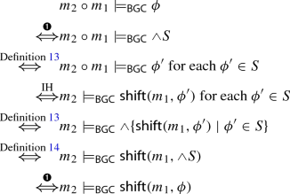
- \(\bullet \):
-
 (➊):
(➊):Fix
 and
and  .
. - \(\bullet \):
-
(Direction 1/2)
Assume: \(m_2\models _{\mathsf {BGC}} {\textsf {shift} } (m_1,\phi ) \) (➋).
We need to show: \(m_2\circ m_1\models _{\mathsf {BGC}} \phi \)


- \(\bullet \):
-
(Direction 2/2) Assume: \(m_2\circ m_1\models _{\mathsf {BGC}} \phi \) (➋). We need to show: \(m_2\models _{\mathsf {BGC}} {\textsf {shift} } (m_1,\phi ) \)


- \(\bullet \):
-
 (➊): Fix
  and
and  .
. 
 and
and  .
. 
 and
and  .
. 
 (➊):
(➊): and
and  .
. 


 (➊): Fix
  and
and  .
. 
\(\square \)
Proof
(Theorem 3, p. 12: Soundness of \({\textsf {enc} }_{\nu }\)) By induction on \(\phi \) and using that \(m\models _{\mathsf {BGC}} {\textsf {shift} } (f,\phi ) \) iff \(m\circ f\models _{\mathsf {BGC}} \phi \) due to Theorem 2. \(\square \)
Proof
(Corollary 1, p. 12: Soundness of \({\textsf {enc} }_{\nu }\) for Graphs) Follows directly from Theorem 3.\(\square \)
Proof
(Theorem 6, p. 58: Soundness of the Operational Satisfaction Check) We show the following stronger property that explains the construction of \(m'\) from m and \(\sigma \) and vice versa of m and \(\sigma \) from \(m'\).

Hence, the partially injective morphism m used for the satisfaction invariantly describes a suitable variable substitution \(\sigma \) that can be used to satisfy the AC returned by \({\textsf {check} }_{\textsf {BGC} } \).
Note that ➊ guarantees that \(m'\) is well-defined and vice versa that the \(\sigma \) obtained from \(m'\) satisfies ➊.
Hence, we only have to show ➋ iff ➌.
By induction on \(\bar{\phi }\).
-
\(\bar{\phi }=\wedge S \):

-
\(\bar{\phi }=\lnot \phi \):

-
 :
: 
-
 :
: 


 :
: 
 :
: 
Proof
(Corollary 3, p. 58: Soundness of the Operational Satisfaction Check for Graphs) Follows directly from Theorem 6.\(\square \)
Proof
(Theorem 4, p. 25: Soundness of \({\textsf {enc} }_{\Delta }\)) By induction on the structure of \(\bar{\phi }\). The proof is trivial for the cases of conjunction, negation, and restriction as these operators are syntactically and semantically preserved. We therefore only consider the case of the \(\Delta \) operator.
Note that in both directions, we basically use the same diagram. On the one hand, when the GC is satisfied, there are jointly epimorphic morphisms constructed using the operation \({\textsf {overlap} }\) that determine a minimal object \(K'\) that can be embedded into the host graph G. On the other hand, each such overlapping can be used to prove that the BGC resulting from encoding is satisfied when the given GC was satisfied.
- \(\bullet \):
-
(Direction 1/2) Assume that \(\bar{\phi }\in \mathcal {S}^{\mathsf {GC}} _{H} \), \(\bar{\phi }=\Delta ^{}(\rho ,\phi ) \),
 ,
,  , and
, and  , and \(m\models _{\mathsf {GC}} \bar{\phi } \).
We have to show that \(m\models _{\mathsf {BGC}} {\textsf {enc} }_{\Delta } (\bar{\phi }) \).
By definition of the GL satisfaction relation we have that there is some
 s.t.
s.t. - \(\bullet \):
-
\(m\circ {\rho }{.}{{\textsf {res} }} =m'\circ {\rho }{.}{{\textsf {ext} }} \),
- \(\bullet \):
-
\(m\models _{\mathsf {BGC}} {\rho }{.}{{\textsf {lC} }} \),
- \(\bullet \):
-
\(m'\models _{\mathsf {BGC}} {\rho }{.}{{\textsf {rC} }} \),
- \(\bullet \):
-
 maps to the set V of variables over which \({\rho }{.}{{\textsf {ac} }} \) is defined,
 - \(\bullet \):
-
 is the unique mapping induced by the universal property of the coproduct of the restriction-extension pattern where \(({m}{.}{{\textsf {X} }},{m'}{.}{{\textsf {X} }})\) are used for comparison,
 - \(\bullet \):
-
\({\textsf {sat} }_{\forall } ({G}{.}{{\textsf {ac} }} \rightarrow \sigma _{ VG }({\rho }{.}{{\textsf {ac} }})) \), and
- \(\bullet \):
-
\(m'\models _{\mathsf {GC}} \phi \).
It is sufficient to show that there is some \((\bar{r},\bar{\ell })\in S\) such that \(m\models _{\mathsf {BGC}} {\rho }{.}{{\textsf {lC} }} \wedge \exists (\bar{\ell },\nu (\bar{r}, {\textsf {enc} }_{\Delta } (\phi ) \wedge {\rho }{.}{{\textsf {rC} }} )) \) where \((\bar{\ell },\bar{r})\in S\), if
- \(\bullet \):
-
 ,
, - \(\bullet \):
-
 ,
, - \(\bullet \):
-
 ,
, - \(\bullet \):
-
 ,
, - \(\bullet \):
-
 ,
, - \(\bullet \):
-
 ,
, - \(\bullet \):
-
 ,
, - \(\bullet \):
-
\(\sigma \circ {\rho }{.}{{\textsf {lX} }} ={\ell '}{.}{{\textsf {X} }}_{\textsf {P} } \),
- \(\bullet \):
-
\(\sigma \circ {\rho }{.}{{\textsf {rX} }} ={r'}{.}{{\textsf {X} }}_{\textsf {P} } \),
- \(\bullet \):
-
\({K''}{.}{{\textsf {ac} }} =\sigma ({\rho }{.}{{\textsf {ac} }} {})\), and
- \(\bullet \):
-
\((\bar{\ell },\bar{r})=(i\circ \ell ',i\circ r')\).
We have the span as in Fig. 18. We can construct \((\ell ',r',\bar{m})\) using \({\textsf {overlap} } \) as an \(\mathcal {E}' \text {-}\mathcal {P} \) -pair-factorization of \((m,m')\). Hence \(m=\bar{m}\circ \ell '\) and \(m'=\bar{m}\circ r'\). We now construct \(K''\) as required via \(i={\textsf {acInc} } (K'') \) and \({K''}{.}{{\textsf {ac} }} =\sigma ({\rho }{.}{{\textsf {ac} }} {})\). We are then able to decompose \(\bar{m}\) into i and h where h maps elements according to \(\bar{m}\) (i.e., \(\bar{m}=h\circ i\)).
Also, h satisfies the AC implication \({\textsf {sat} }_{\forall } ({G}{.}{{\textsf {ac} }} \rightarrow {h}{.}{{\textsf {X} }} ({K''}{.}{{\textsf {ac} }})) \)
because \({\textsf {sat} }_{\forall } ({G}{.}{{\textsf {ac} }} \rightarrow {h}{.}{{\textsf {X} }} (\sigma ({\rho }{.}{{\textsf {ac} }} {}))) \)
because \({\textsf {sat} }_{\forall } ({G}{.}{{\textsf {ac} }} \rightarrow \sigma _{ VG }({\rho }{.}{{\textsf {ac} }})) \) (from above)
and because \({h}{.}{{\textsf {X} }} \circ \sigma =\sigma _{ VG }\) due to the universal property of the coproduct.
Also note that \(m=h\circ i\circ \ell '\) and \(m'=h\circ i\circ r'\).
Also, m satisfies \({\rho }{.}{{\textsf {lC} }} \) as assumed.
Then, m satisfies \(\exists (\bar{\ell },\nu (\bar{r}, {\textsf {enc} }_{\Delta } (\phi ) \wedge {\rho }{.}{{\textsf {rC} }} )) \) because
\(\bar{m}=h\circ i\) satisfies \(\nu (\bar{r}, {\textsf {enc} }_{\Delta } (\phi ) \wedge {\rho }{.}{{\textsf {rC} }} ) \) because
\(m'\) satisfies \( {\textsf {enc} }_{\Delta } (\phi ) \wedge {\rho }{.}{{\textsf {rC} }} \) by assumption.

- \(\bullet \):
-
(Direction 2/2) Assume that \(\bar{\phi }\in \mathcal {S}^{\mathsf {GC}} _{H} \), \(\bar{\phi }=\Delta ^{}(\rho ,\phi ) \),
 ,
,  , and
, and  , and there is such a morphism pair \((\bar{\ell },\bar{r})\) such that
\(m\models _{\mathsf {BGC}} {\rho }{.}{{\textsf {lC} }} \wedge \exists (\bar{\ell },\nu (\bar{r}, {\textsf {enc} }_{\Delta } (\phi ) \wedge {\rho }{.}{{\textsf {rC} }} )) \) and
- \(\bullet \):
-
 ,
, - \(\bullet \):
-
 ,
, - \(\bullet \):
-
 ,
, - \(\bullet \):
-
 ,
, - \(\bullet \):
-
 ,
, - \(\bullet \):
-
 ,
, - \(\bullet \):
-
 ,
, - \(\bullet \):
-
\(\sigma \circ {\rho }{.}{{\textsf {lX} }} ={\ell '}{.}{{\textsf {X} }}_{\textsf {P} } \),
- \(\bullet \):
-
\(\sigma \circ {\rho }{.}{{\textsf {rX} }} ={r'}{.}{{\textsf {X} }}_{\textsf {P} } \),
- \(\bullet \):
-
\({K''}{.}{{\textsf {ac} }} =\sigma ({\rho }{.}{{\textsf {ac} }} {})\), and
- \(\bullet \):
-
\((\bar{\ell },\bar{r})=(i\circ \ell ',i\circ r')\).
We have to show \(m\models _{\mathsf {GC}} \bar{\phi } \).
We have that \(m\models _{\mathsf {BGC}} {\rho }{.}{{\textsf {lC} }} \) and that there is some
 with \(h\circ \bar{\ell }=h\circ i\circ \ell '=m\) and \(h\models _{\mathsf {BGC}} \nu (\bar{r}, {\textsf {enc} }_{\Delta } (\phi ) \wedge {\rho }{.}{{\textsf {rC} }} ) \).
Hence, \(h\circ \bar{r}\models _{\mathsf {BGC}} {\textsf {enc} }_{\Delta } (\phi ) \wedge {\rho }{.}{{\textsf {rC} }} \).
Hence, \(h\circ \bar{r}\models _{\mathsf {BGC}} {\textsf {enc} }_{\Delta } (\phi ) \) and \(h\circ \bar{r}\models _{\mathsf {BGC}} {\rho }{.}{{\textsf {rC} }} \).
By definition of the GL satisfaction relation we have to show that there is some
 s.t.
s.t. - \(\bullet \):
-
\(m\circ {\rho }{.}{{\textsf {res} }} =m'\circ {\rho }{.}{{\textsf {ext} }} \),
- \(\bullet \):
-
\(m\models _{\mathsf {BGC}} {\rho }{.}{{\textsf {lC} }} \),
- \(\bullet \):
-
\(m'\models _{\mathsf {BGC}} {\rho }{.}{{\textsf {rC} }} \),
- \(\bullet \):
-
 maps to the set V of variables over which \({\rho }{.}{{\textsf {ac} }} \) is defined,
 - \(\bullet \):
-
 is the unique mapping induced by the universal property of the coproduct of the restriction-extension pattern where \(({m}{.}{{\textsf {X} }},{m'}{.}{{\textsf {X} }})\) are used for comparison,
 - \(\bullet \):
-
\({\textsf {sat} }_{\forall } ({G}{.}{{\textsf {ac} }} \rightarrow \sigma _{ VG }({\rho }{.}{{\textsf {ac} }})) \), and
- \(\bullet \):
-
\(m'\models _{\mathsf {GC}} \phi \).
We choose \(m'\) to be \(h\circ i\circ r'\), which is equal to \(h\circ \bar{r}\).
We have that \(m\circ {\rho }{.}{{\textsf {res} }} =h\circ i\circ \ell '\circ {\rho }{.}{{\textsf {res} }} =h\circ i\circ r'\circ {\rho }{.}{{\textsf {ext} }} =m'\circ {\rho }{.}{{\textsf {ext} }} \) using \(m=h\circ i\circ \ell '\) and \(\ell '\circ {\rho }{.}{{\textsf {res} }} =r'\circ {\rho }{.}{{\textsf {ext} }} \) (due to the use of \({\textsf {overlap} }\)), and our selection of \(m'\).
\(m\models _{\mathsf {BGC}} {\rho }{.}{{\textsf {lC} }} \) is satisfied as obtained before.
\(m'\models _{\mathsf {BGC}} {\rho }{.}{{\textsf {rC} }} \) is satisfied because \(h\circ i\circ r'\models _{\mathsf {BGC}} {\rho }{.}{{\textsf {rC} }} \) is satisfied as obtained before with \(\bar{r}=i\circ r'\).
\({\rho }{.}{{\textsf {lX} }} \) can be constructed as described.
\({\textsf {sat} }_{\forall } ({G}{.}{{\textsf {ac} }} \rightarrow \sigma _{ VG }({\rho }{.}{{\textsf {ac} }})) \) because \({\textsf {sat} }_{\forall } ({G}{.}{{\textsf {ac} }} \rightarrow {h}{.}{{\textsf {X} }} (\sigma ({\rho }{.}{{\textsf {ac} }} {}))) \) because \({\textsf {sat} }_{\forall } ({G}{.}{{\textsf {ac} }} \rightarrow {h}{.}{{\textsf {X} }} ({K''}{.}{{\textsf {ac} }})) \) because h is a morphism and because \({h}{.}{{\textsf {X} }} \circ \sigma =\sigma _{ VG }\) due to the universal property of the coproduct. \(\square \)

 ,
,  , and
, and  , and
, and  s.t.
s.t.  maps to the set V of variables over which
  is the unique mapping induced by the universal property of the coproduct of the restriction-extension pattern where
  ,
, ,
, ,
, ,
, ,
, ,
, ,
,
 ,
,  , and
, and  , and there is such a morphism pair
  ,
, ,
, ,
, ,
, ,
, ,
, ,
, with
with  s.t.
s.t.  maps to the set V of variables over which
  is the unique mapping induced by the universal property of the coproduct of the restriction-extension pattern where
Proof
(Corollary 2, p. 25: Soundness of \({\textsf {enc} }_{\Delta }\) for Graphs) Trivially from Theorem 4.\(\square \)
Proof
(Theorem 5, p. 45: Soundness of  ) The proof proceeds by induction on the structure of the MTGC that is translated where the cases of conjunction and negation are trivial and omitted here. Hence, we only consider the operations delta-lock and delta-release. However, to avoid an overly technical presentation, we focus on each of the items in the reduction individually.
- \(\bullet \):
-
delta-lock:
- \(\bullet \):
-
input metric temporal graph condition \(\psi \):
- \(\bullet \):
-
 ,
, - \(\bullet \):
-
\({\theta _1}{.}{{\textsf {lG} }} ={\theta _2}{.}{{\textsf {lG} }} =H\),
- \(\bullet \):
-
\({\theta _1}{.}{{\textsf {rG} }} =H_1'\),
- \(\bullet \):
-
\({\theta _2}{.}{{\textsf {rG} }} =H_2'\),
- \(\bullet \):
-
consistency rule \(\theta _2'\):
- \(\bullet \):
-
\(x_2\notin V\),
The check ensures that the variable \(x_2\) is not confused with the other variables introduced before.
- \(\bullet \):
-
\(\theta _2'={\textsf {ruleAdd} } (H,V,x_2,{\textsf {shift} }_{\textsf {DS} } (\gamma ,x_2, x_{outer} )) \),
The created rule checks for the existence of a timepoint given by \(x_2\) in the duration specification \(\gamma \) relative to the previous variable \( x_{outer} \).
- \(\bullet \):
-
evolution pattern \(\theta _2''\):
- \(\bullet \):
-
\(\gamma _2''={\textsf {alive} }({{x_2}, {H_2'}})\)
\(\wedge \,\,{(\mathsf {if~} \kappa =\mathsf {N} \mathsf {~then~}}{{ {{\textsf {earliest} }(x_2,H_2')} }\,\,{\text {else}}\,\,{ \top } ) }\),
The AC checks whether the elements matched for \(H_2'\) are alive w.r.t. the chosen timepoint \(x_2\). For the case of \(\kappa =\mathsf {N} \) it also checks whether one of the graph elements in \(H_2'\) is just created at timepoint \(x_2\).
- \(\bullet \):
-
\(\theta _2''={\textsf {ruleExt} } (\theta _2,V\cup \{x_2\},\gamma _2'') \),
The rule \(\theta _2\) is extended to also check for the stated AC \(\gamma _2''\).
- \(\bullet \):
-
graph condition \(\phi _2\):
- \(\bullet \):
-
 ,
,We apply the encoding inductively.
- \(\bullet \):
-
evolution pattern \(\theta _1'\):
- \(\bullet \):
-
\(x_1\notin V\),
The check ensures that the variable \(x_2\) is not confused with the other variables introduced before.
- \(\bullet \):
-
\(\gamma _1= x_2< x_1 \wedge x_1\le x_{outer} \),
Hence, we check for the condition \(\delta '\in (\delta ,0]\) from the satisfaction relation.
- \(\bullet \):
-
\(\gamma _2= x_{outer} \le x_1 \wedge x_1< x_2 \),
Hence, we check for the condition \(\delta '\in [0,\delta )\) from the satisfaction relation.
- \(\bullet \):
-
\(\theta _1'={\textsf {ruleAdd} } (H,V\cup \{x_2\},x_1,\gamma _1\vee \gamma _2) \),
The created rule checks for the existence of a timepoint given by \(x_1\) that satisfies one of the two ACs \(\gamma _1\) and \(\gamma _2\) from above. Hence, we check for the condition \(\delta '\in (\delta ,0]\cup [0,\delta )\) from the satisfaction relation.
- \(\bullet \):
-
evolution pattern \(\theta _1''\):
- \(\bullet \):
-
\(\theta _1''={\textsf {ruleExt} } (\theta _1,V \cup \{x_2,x_1\},{{\textsf {alive} }(x_1,H_1')}) \),
The rule \(\theta _1\) is extended to also check for whether the graph elements matched for \(H_1'\) are all alive for the timepoint given by \(x_1\).
- \(\bullet \):
-
graph condition \(\phi _1\):
- \(\bullet \):
-
 ,
,We apply the encoding inductively.
- \(\bullet \):
-
evolution pattern \(\bar{\theta }_2'\):
- \(\bullet \):
-
\(\bar{x}_2\notin V\),
The check ensures that the variable \(x_2\) is not confused with the other variables introduced before.
- \(\bullet \):
-
\(\bar{\gamma }_1= x_2< \bar{x}_2 \wedge \bar{x}_2\le x_{outer} \),
Hence, we check for the condition \(\delta '\in (\delta ,0]\) from the satisfaction relation.
- \(\bullet \):
-
\(\bar{\gamma }_2= x_{outer} \le \bar{x}_2 \wedge \bar{x}_2< x_2 \),
Hence, we check for the condition \(\delta '\in [0,\delta )\) from the satisfaction relation.
- \(\bullet \):
-
\(\bar{\gamma }_3= (\bar{\gamma }_1\vee \bar{\gamma }_2) \wedge {\textsf {shift} }_{\textsf {DS} } (\gamma ,\bar{x}_2, x_{outer} ) \),
Hence, we check for the condition \(\delta '\in ((\delta ,0]\cup [0,\delta )) \cap {\textsf {sem} }(\gamma ) \) from the satisfaction relation.
- \(\bullet \):
-
\(\bar{\theta }_2'={\textsf {ruleAdd} } (H,V\cup \{x_2\},\bar{x}_2,\bar{\gamma }_3) \),
The created rule checks for the existence of a timepoint given by \(\bar{x}_2\) that satisfies the AC \(\bar{\gamma }_3\).
- \(\bullet \):
-
evolution pattern \(\bar{\theta }_2''\):
- \(\bullet \):
-
\(\bar{\theta }_2''={\textsf {ruleExt} } (\theta _2,V \cup \{x_2,\bar{x}_2\},{{\textsf {alive} }(\bar{x}_2,H_2')}) \),
The rule \(\theta _2\) is extended to also check for whether the graph elements matched for \(H_2'\) are all alive for the timepoint given by \(\bar{x}_2\).
- \(\bullet \):
-
graph condition \(\bar{\phi }_2\):
- \(\bullet \):
-
\(\bar{\phi }_2= \mathsf {if~}\kappa =\mathsf {C} \mathsf {~then~} \Delta ^{\mathsf {A}}(\bar{\theta }_2',\lnot \Delta ^{\mathsf {E}}(\bar{\theta }_2'',\top ) ) \mathsf {~else~}{ \top }\),
The check that no timepoints described by \(\gamma \) are closer to t (given by \( x_{outer} \)) than \(\delta \) (given by \(x_2\)) (in the future or past direction) permits the same match.
- \(\bullet \):
-
output graph condition \(\phi \):
 ,
, ,
, ,
,- \(\bullet \):
-
\(\phi = \Delta ^{\mathsf {E}}(\theta _2', \Delta ^{\mathsf {E}}(\theta _2'',\phi _2) \wedge \Delta ^{\mathsf {A}}(\theta _1',\Delta ^{\mathsf {E}}(\theta _1'',\phi _1)) \wedge \bar{\phi }_2 ) \).
The check that there is a timepoint \(\theta _2'\) such that the right-hand side argument \(\Delta ^{\mathsf {E}}(\theta _2'',\phi _2) \) is satisfied and such that for all timepoints in \(\theta _1'\) the left-hand side argument \(\Delta ^{\mathsf {E}}(\theta _1'',\phi _1) \) is satisfied.
- \(\bullet \):
-
delta-release:
- \(\bullet \):
-
input metric temporal graph condition \(\psi \):
- \(\bullet \):
-
\(\psi =\boxdot (\bar{\theta },\bar{\psi }) \),
- \(\bullet \):
-
\({\bar{\theta }}{.}{{\textsf {lG} }} =H\),
- \(\bullet \):
-
\({\bar{\theta }}{.}{{\textsf {rG} }} =H'\),
- \(\bullet \):
-
\( xs = xs' \cdot x_{last} \),
- \(\bullet \):
-
consistency rule \(\bar{\theta }'\):
- \(\bullet \):
-
\(x\notin V\),
The check ensures that the variable \(x_2\) is not confused with the other variables introduced before.
- \(\bullet \):
-
\(\gamma _1= x_{last} \le x \wedge x< x_{outer} \),
Hence, we check for \([t',t)\) from the satisfaction relation.
- \(\bullet \):
-
\(\gamma _2= x_{outer} < x \wedge x\le x_{last} \),
Hence, we check for \((t,t']\) from the satisfaction relation.
- \(\bullet \):
-
\(\bar{\theta }'={\textsf {ruleAdd} } (H,V,x,\gamma _1\vee \gamma _2) \),
The created rule checks for the existence of a timepoint given by x that satisfies one of the two ACs \(\gamma _1\) and \(\gamma _2\). Hence, we check for \([t',t)\cup (t,t']\) from the satisfaction relation.
- \(\bullet \):
-
consistency rule \(\bar{\theta }''\):
- \(\bullet \):
-
\(\bar{\theta }''={\textsf {ruleExt} } (\bar{\theta },V\cup \{x\},{{\textsf {alive} }(x,H')}) \),
The rule \(\bar{\theta }\) is extended to also check for whether the graph elements matched for \(H'\) are all alive for the timepoint given by x.
- \(\bullet \):
-
graph condition \(\bar{\phi }\):
- \(\bullet \):
-
 ,
,We apply the encoding inductively.
 ,
,- \(\bullet \):
-
output graph condition \(\phi \):
- \(\bullet \):
-
\(\phi = \Delta ^{\mathsf {A}}(\bar{\theta }', \Delta ^{\mathsf {E}}(\bar{\theta }'',\bar{\phi })) \).
The check that for all timepoints in between the current timepoint and the former timepoint \(\bar{\theta }'\), the translated subcondition \(\Delta ^{\mathsf {E}}(\bar{\theta }'',\bar{\phi }) \) is satisfied.
This relationship between the satisfaction relation of MTGL and the translated GC demonstrates the corresponding encoding of timepoints using additional global variables that are quantified and restricted according to the quantifiers and intervals specified in the satisfaction relation of MTGL.\(\square \)
E Glossary
Section 2 (p. 4): Attribute Logic AL
Further entries regarding AL are listed below in “Appendix A”.
-
\(\mathcal {S}^{{\textsf {AC} }} _{ Var } \) , all attribute conditions (ACs)
-
\(\mathcal {V} \), all values
-
\(\alpha \models _{\mathsf {AC}} \gamma \), satisfaction of ACs
-
\({\textsf {sat} }_{\forall } (\gamma ) \), tautological AC
-
\({\textsf {sat} }_{\exists } (\gamma ) \), satisfiable AC
Section 3 (p. 4): Symbolic Graphs
-
\({f}{.}{{\textsf {X} }} \), mapping of all variables, Definition 2, p. 6
-
\({f}{.}{{\textsf {X} }}_{\mathcal {V}} \), mapping of all variables and values, Definition 2, p. 6
-
\({f}{.}{{\textsf {X} }}_{\textsf {GM} } \), mapping of variables to values, Definition 2, p. 6
-
\({f}{.}{{\textsf {X} }}_{\textsf {P} } \), mapping of variables when \({f}{.}{{\textsf {X} }}_{\textsf {GM} } =\varnothing \), Definition 2, p. 6
-
\(\mathbf {Graphs} \), all (finite) graphs typed over \( TG \), Definition 4, p. 7
-
 , a graph morphism, Definition 5, p. 7
 -
 , inclusion morphism, below of Definition 6, p. 7
 -
 , identity morphism, below of Definition 6, p. 7
 -
\(\varvec{\varnothing } \), the empty graph, below of Theorem. 1, p. 7
-
 , initial morphism, above of Definition 7, p. 7
 -
 , a monomorphism, below of Definition 7, p. 7
 -
\(\mathcal {M} \), all monomorphisms, below of Definition 7, p. 7
-
 , an epimorphism, below of Definition 7, p. 8
 -
\(\mathcal {E} \), all epimorphisms, below of Definition 7, p. 8
-
 , an isomorphism, below of Definition 7, p. 8
 -
\(\mathcal {E}' \), all pairs of jointly epimorphic morphisms, below of Definition 7, p. 8
-
 , an AC inclusion morphism Definition 8, p. 8
 -
 , a partially injective morphism, Definition 7, p. 7
 -
\(\mathcal {P} \), all partially injective morphisms, Definition 7, p. 7
-
\({\textsf {grounded} } (G) \), the grounded graph predicate, Definition 9, p. 8
-
\({\textsf {induced-grounded} } (G) \), all grounded graphs that are induced by G, Definition 10, p. 8
-
\({\textsf {overlap} } (f,m) \), operation for graph overlapping, Definition 11, p. 8
-
 , a global -,variable partial-, substitution morphism, Definition 59, p. 55
 , a graph morphism, Definition
  , inclusion morphism, below of Definition
  , identity morphism, below of Definition
  , initial morphism, above of Definition
  , a monomorphism, below of Definition
  , an epimorphism, below of Definition
  , an isomorphism, below of Definition
  , an AC inclusion morphism Definition
  , a partially injective morphism, Definition
  , a global -,variable partial-, substitution morphism, Definition
 Section 4 (p. 9): Basic Graph Logic
-
\(\mathcal {S}^{\mathsf {BGC}} _{H} \), all basic graph conditions (BGCs) \(\phi \) over H, Definition 12, p. 9
-
\(m\models _{\mathsf {BGC}} \phi \), satisfaction relation for BGL w.r.t. a morphism, Definition 13, p. 10
-
\(G\models _{\mathsf {BGC}} \phi \), satisfaction relation for BGL w.r.t. a graph, Definition 13, p. 10
-
\({\textsf {shift} } \), operation for shifting a BGC over a monomorphism, Definition 14, p. 11
-
\({\textsf {enc} }_{\nu } \), operation for encoding the BGL operator restrict using \({\textsf {shift} } \), Definition 15, p. 12
-
\({\textsf {check} }_{\textsf {BGC} } \), operation for checking the satisfaction of BGCs w.r.t. morphisms, Definition 60, p. 58
Section 5 (p. 12): Graph Transformation
-
\(\mathcal {S}^{\mathsf {rules}} \), all finite rules \(\rho \), Definition 16, p. 14
-
\({\textsf {id} } \), an identity rule, Definition 17, p. 14
-
 , a graph transformation step, Definition 18, p. 17
 -
\(\mathcal {S}^{\mathsf {steps}} \), all step labels \(\varsigma \), Definition 18, p. 17
-
\(\Pi _{G} \), all graph sequences \(\pi \) starting in graph G, Definition 19, p. 17
-
\({\textsf {length} }(\pi ) \), the length of the graph sequence \(\pi \), Definition 19, p. 17
-
\(\Pi ^{\mathsf {fin}}_{G} \), all finite graph sequences that are starting in graph G, Definition 19, p. 17
-
\(\pi ^{\mathsf {G}}(k) \), the graph in the graph sequence \(\pi \) at index k, Definition 19, p. 17
-
\(\Pi ^{\mathsf {fin}}_{G,H} \), all graph sequences that are starting in graph G and ending in graph H, Definition 19, p. 17
-
\({\textsf {rev} }(\pi ) \), the reversal of a graph sequence, Definition 19, p. 17
-
\( time \), a function mapping a graph to a global time, Definition 20, p. 18
-
\(\Pi ^{ time }_{G} \), all timed graph sequences (TGSs) \(\pi \) that are starting in graph G, Definition 20, p. 18
-
\(\Pi ^{\mathsf {fin}, time }_{G} \), all finite TGSs that are starting in graph G, Definition 20, p. 18
-
\({\textsf {dur} }(\pi ) \), the duration of a TGS in time units, Definition 20, p. 18
-
\(\pi ^{\mathsf {T}}(t) \), the graph in the TGS \(\pi \) at timepoint t, Definition 20, p. 18
-
\(\pi ^{\mathsf {T}}(\{t_1,t_2\}) \), the TGS contained in \(\pi \) between the timepoints \(t_1\) and \(t_2\), Definition 20, p. 18
-
\(\mathcal {S}^{\mathsf {gts}} \), all graph transformation systems S, Definition 21, p. 18
-
\(\mathcal {S}^{\mathsf {gts\cdot s}}_{S} \), all graph sequences generated by a graph transformation system S, Definition 22, p. 22
-
\(\mathcal {S}^{\mathsf {tgts}}_{ time } \), all timed graph transformation systems S, Definition 23, p. 22
-
\(\mathcal {S}^{\mathsf {tgts\cdot s}}_{S} \), all TGSs generated by a timed graph transformation system S, Definition 24, p. 22
 , a graph transformation step, Definition
 Section 6 (p. 22): Graph Logic
-
\(\mathcal {S}^{\mathsf {REP}} \), all finite restriction-extension patterns \(\rho \), Definition 25, p. 22
-
\(\mathcal {S}^{\mathsf {GC}} _{H} \), all graph conditions (GCs) \(\phi \) over H, Definition 26, p. 23
-
\(m\models _{\mathsf {GC}} \phi \), satisfaction relation for GL w.r.t. a morphism, Definition 27, p. 23
-
\(G\models _{\mathsf {GC}} \phi \), satisfaction relation for GL w.r.t. a graph, Definition 27, p. 23
-
\({\textsf {enc} }_{\Delta } \), operation for encoding the GL operator delta , Definition 28, p. 25
Section 7 (p. 25): Metric Temporal Graph Logic
-
\(\mathcal {S}^{\mathsf {EP}} \), all finite evolution patterns \(\theta \), Definition 29, p. 27
-
\({\textsf {admissible-comatches}}{((\ell ,r)},{m},{\theta })\), operation for deriving the set of all admissible comatches for a span, a match, and an evolution pattern, Definition 30, p. 30
-
\({\textsf {derivedSpan} }(\pi ) \), the derived span of a finite graph sequence, Definition 31, p. 30
-
\({\textsf {PM} } (\pi ,m,\theta ) \), the propagation of a match m over a TGS for an evolution pattern, Definition 32, p. 30
-
\({\textsf {PM} } (\pi ,t_1,t_2,m,\theta ) \), the propagation of a match m between two timepoints in a TGS for an evolution pattern, Definition 33, p. 32
-
\(\mathcal {S}^{{\textsf {AC} }} _{{\textsf {DS} }(\tau )} \), all duration specifications \(\gamma \) over a variable \(\tau \), Definition 34, p. 34
-
\({\textsf {sem} }(\gamma ) \), the induced semantics of a duration specification: a set of timepoints, Definition 34, p. 34
-
\({\textsf {shift} }_{\textsf {DS} } (\gamma ,x,y) \), operation for shifting a duration specification to some timepoint, Definition 34, p. 34
-
\({\mathcal {S}}_{n, H}^{\mathsf {MTGC}}\), all metric temporal graph conditions (MTGCs) \(\psi \) over a graph H with n return timepoints, Definition 35, p. 35
-
\((\pi , ts ,t,m)\models _{\text {MTGC}} \psi \), satisfaction relation for MTGL w.r.t. a TGS, a list of timepoints, a timepoint, and a morphism, Definition 36, p. 39
-
\(\pi \models _{\text {MTGC}} \psi \), satisfaction relation for MTGL w.r.t. a TGS , Definition 36, p. 39
-
\(\text {GH} \), a graph with history, Definition 37, p. 40
-
\({\textsf {Fold} }^{\textsf {1st} } \), operation for obtaining the GH for the first graph of a TGS , Definition 38, p. 41
-
\({\textsf {Fold} }^{\textsf {span} } \), operation for updating a GH according to a span, Definition 39, p. 41
-
\({\textsf {Fold} }^{\textsf {tgs} } \), operation for incrementally folding an entire finite TGS , Definition 40, p. 41
-
\({{\textsf {alive} }} \), operation for constructing an AC that requires that all graph elements are alive at a certain timepoint, Definition 41, p. 43
-
\({{\textsf {earliest} }} \), operation for constructing an AC that requires that at least one graph element has the given largest creation timepoint, Definition 42, p. 43
-
\({\textsf {ruleAdd} } \), operation for constructing an evolution pattern for quantifying over an additional global variable, Definition 43, p. 43
-
\({\textsf {ruleExt} } \), operation for extending a given evolution pattern to subsume additional elements, Definition 44, p. 44
-
 , operation for encoding the MTGL operators delta-lock and delta-release , Definition 45, p. 44
 , operation for encoding the MTGL operators delta-lock and delta-release , Definition
 Appendix A (p. 51): Details for Attribute Logic AL
-
\(\mathcal {S}^{{\textsf {sigs} }}_{} \), all signatures, Definition 46, p. 52
-
\(\mathcal {S}^{{\textsf {vars} }}_{\Sigma } \), all variable systems, Definition 47, p. 52
-
\(\mathcal {S}^{{\textsf {terms} }}_{\Sigma {,s}}{( Var )} \), all terms, Definition 48, p. 52
-
\({\textsf {Sub} }_{\Sigma , Var _1, Var _2} \), all variable substitutions, Definition 49, p. 53
-
\(\mathcal {S}^{{\textsf {specs} }}_{\Sigma , Var } \), all algebraic specifications, Definition 50, p. 53
-
\(\equiv \), equivalence of terms, Definition 51, p. 53
-
\(\cong \), congruence of terms, Definition 52, p. 53
-
\(\sigma \models _{\mathsf {SP}} t \), satisfaction of Boolean terms, Definition 53, p. 54
-
\(\mathcal {S}^{{\textsf {AC} }} _{ Var } \), all attribute conditions (ACs), Definition 54, p. 54
-
\({\textsf {fv} } (\gamma ) \), free variables of ACs , Definition 55, p. 54
-
\(\mathcal {V} \), all values of a signature, Definition 56, p. 54
-
\({\textsf {Val} }_{\Sigma , Var } \), all variable valuations, Definition 57, p. 54
-
\(\alpha \models _{\mathsf {AC}} \gamma \), satisfaction of ACs , Definition 58, p. 54
-
\({\textsf {sat} }_{\forall } (\gamma ) \), tautological AC , Definition 58, p. 54
-
\({\textsf {sat} }_{\exists } (\gamma ) \), satisfiable AC , Definition 58, p. 54
Rights and permissions
Open Access This article is licensed under a Creative Commons Attribution 4.0 International License, which permits use, sharing, adaptation, distribution and reproduction in any medium or format, as long as you give appropriate credit to the original author(s) and the source, provide a link to the Creative Commons licence, and indicate if changes were made. The images or other third party material in this article are included in the article’s Creative Commons licence, unless indicated otherwise in a credit line to the material. If material is not included in the article’s Creative Commons licence and your intended use is not permitted by statutory regulation or exceeds the permitted use, you will need to obtain permission directly from the copyright holder. To view a copy of this licence, visit http://creativecommons.org/licenses/by/4.0/.
About this article

Cite this article
Schneider, S., Maximova, M., Sakizloglou, L. et al. Formal testing of timed graph transformation systems using metric temporal graph logic. Int J Softw Tools Technol Transfer 23, 411–488 (2021). https://doi.org/10.1007/s10009-020-00585-w
Published:
Issue Date:
DOI: https://doi.org/10.1007/s10009-020-00585-w