
Abstract
To help users get familiar with large RDF graphs, RDF summarization techniques can be used. In this work, we study quotient summaries of RDF graphs, that is: graph summaries derived from a notion of equivalence among RDF graph nodes. We make the following contributions: (i) four novel summaries which are often small and easy-to-comprehend, in the style of E–R diagrams; (ii) efficient (amortized linear-time) algorithms for computing these summaries either from scratch, or incrementally, reflecting additions to the graph; (iii) the first formal study of the interplay between RDF graph saturation in the presence of an RDFS ontology, and summarization; we provide a sufficient condition for a highly efficient shortcut method to build the quotient summary of a graph without saturating it; (iv) formal results establishing the shortcut conditions for some of our summaries and others from the literature; (v) experimental validations of our claim within a tool available online.


Notes
An equivalence relation \(\equiv \) is a binary relation that is reflexive, i.e., \(x \equiv x\), symmetric, i.e., \(x\equiv y\)\(\Rightarrow \)\(y\equiv x\), and transitive, i.e., \(x\equiv y\) and \(y\equiv z\) implies \(x \equiv z\) for any x, y, z.
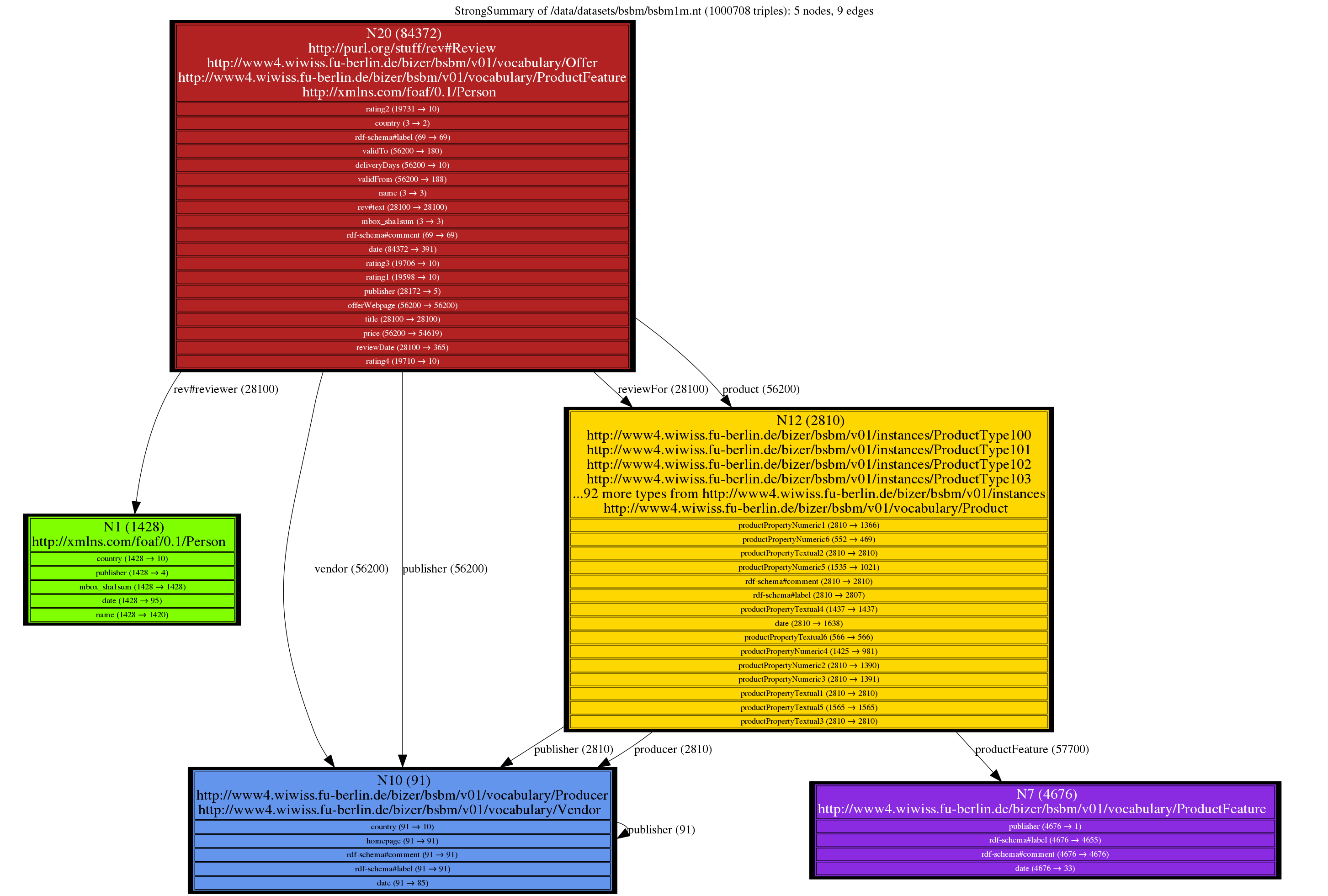
One example among many: the \(\texttt {W}\) summary of a BSBM 1M graph has just one node, whereas the \(\texttt {S}\) summary has 5 and is quite informative (https://rdfquotient.inria.fr/files/2019/11/bsbm1m_s_split_and_fold_leaves.png).
While we consider the ontology very important, our goal is to bring the much more numerous data and type (non-ontology) triples to a visually comprehensible size through summarization. When present, the ontology may help visualize the data; the ontology itself may be summarized, etc.
We exclude a few “standard” root types, such as \(\text {rdfs}\):\(\text {Resource}\) in RDF Schema or \(\text {OWL}\):\(\text {Thing}\), from the supertype hierarchy, as these would not bring useful information to summary users.
Our equivalence relations are defined based on the triples of a given graph \(\texttt {G}\), thus when summarization starts, we do not know whether any two nodes are equivalent; the full equivalence relation is known only after inspecting all \(\texttt {G}\) triples.
In details, for the graphs in Table 4, we omitted: 1008, 4028, 13352, 16020, 19, 1, 5, 246, 246, 246, 171, resp. 108 triples
Note that in the particular case of triples connecting untyped nodes, the algorithms coincide.
References
Abiteboul, S., Hull, R., Vianu, V.: Foundations of Databases. Addison-Wesley, Boston (1995)
Aluç, G., Hartig, O., Özsu, M.T., Daudjee, K.: Diversified stress testing of RDF data management systems. In: ISWC, pp. 197–212 (2014)
Bizer, C., Schultz, A.: The Berlin SPARQL benchmark. Int. J. Semantic Web Inf. Syst. 5(2), 1–24 (2009)
Bohannon, P., Freire, J., Roy, P., Siméon, J.: From XML schema to relations: a cost-based approach to XML storage. In: ICDE (2002)
Campinas, S., Delbru, R., Tummarello, G.: Efficiency and precision trade-offs in graph summary algorithms. In: IDEAS (2013)
Čebirić, Š., Goasdoué, F., Guzewicz, P., Manolescu, I.: Compact summaries of rich heterogeneous graphs. In: Research Report RR-8920, INRIA and U. Rennes 1 (2018). https://hal.inria.fr/hal-01325900v6. See also previous version (v5)
Cebiric, S., Goasdoué, F., Kondylakis, H., Kotzinos, D., Manolescu, I., Troullinou, G., Zneika, M.: Summarizing semantic graphs: a survey. VLDB J 28, 295–327 (2018)
Čebirić, Š., Goasdoué, F., Manolescu, I.: A framework for efficient representative summarization of RDF graphs. In: ISWC (poster) (2017)
Chen, C., Lin, C.X., Fredrikson, M., Christodorescu, M., Yan, X., Han, J.: Mining graph patterns efficiently via randomized summaries. PVLDB 2(1), 742–753 (2009)
Chen, Q., Lim, A., Ong, K.W.: \(D(K)\)-index: An adaptive structural summary for graph-structured data. In: SIGMOD (2003)
Consens, M.P., Miller, R.J., Rizzolo, F., Vaisman, A.A.: Exploring XML web collections with DescribeX. TWEB 4(3), 1–46 (2010)
Deutsch, A., Fernández, M.F., Suciu, D.: Storing semistructured data with STORED. In: SIGMOD (1999)
Fan, W., Li, J., Wang, X., Wu, Y.: Query preserving graph compression. In: SIGMOD (2012)
Galil, Z., Italiano, G.F.: Data structures and algorithms for disjoint set union problems. ACM Comput. Surv. 23(3), 319–344 (1991)
Goasdoué, F., Guzewicz, P., Manolescu, I.: Incremental structural summarization of RDF graphs. In: EDBT. Lisbon (2019). https://hal.inria.fr/hal-01978784
Goasdoué, F., Manolescu, I., Roatiş, A.: Efficient query answering against dynamic RDF databases. In: EDBT (2013)
Goldman, R., Widom, J.: Dataguides: Enabling query formulation and optimization in semistructured databases. In: VLDB (1997)
Gubichev, A., Neumann, T.: Exploiting the query structure for efficient join ordering in SPARQL queries. In: EDBT, pp. 439–450 (2014)
Guo, Y., Pan, Z., Heflin, J.: LUBM: a benchmark for OWL knowledge base systems. J. Web Semant. 3(2–3), 158–182 (2005)
Gurajada, S., Seufert, S., Miliaraki, I., Theobald, M.: Using graph summarization for join-ahead pruning in a distributed RDF engine. In: SWIM Workshop (2014)
Henzinger, M.R., Henzinger, T.A., Kopke, P.W.: Computing simulations on finite and infinite graphs. In: FOCS (1995)
Kaushik, R., Bohannon, P., Naughton, J.F., Korth, H.F.: Covering indexes for branching path queries. In: SIGMOD (2002)
Kaushik, R., Shenoy, P., Bohannon, P., Gudes, E.: Exploiting local similarity for indexing paths in graph-structured data. In: ICDE (2002)
Khan, K., Nawaz, W., Lee, Y.: Set-based approximate approach for lossless graph summarization. Computing 97(12), 1185–1207 (2015)
Khatchadourian, S., Consens, M.P.: ExpLOD: summary-based exploration of interlinking and RDF usage in the linked open data cloud. In: ESWC (2010)
Khatchadourian, S., Consens, M.P.: Constructing bisimulation summaries on a multi-core graph processing framework. In: GRADES Workshop (2015)
Le, W., Li, F., Kementsietsidis, A., Duan, S.: Scalable keyword search on large RDF data. IEEE TKDE 26(11), 2774–2788 (2014)
LeFevre, K., Terzi, E.: GraSS: graph structure summarization. In: SDM (2010)
Liu, Y., Safavi, T., Dighe, A., Koutra, D.: Graph summarization methods and applications: a survey. ACM Comput. Surv. 51(3), 1–34 (2018)
Milo, T., Suciu, D.: Index structures for path expressions. In: ICDT (1999)
Navlakha, S., Rastogi, R., Shrivastava, N.: Graph summarization with bounded error. In: SIGMOD (2008)
Neumann, T., Moerkotte, G.: Characteristic sets: Accurate cardinality estimation for RDF queries with multiple joins. In: ICDE (2011)
Principe, R.A.A., Spahiu, B., Palmonari, M., Rula, A., Paoli, F.D., Maurino, A.: ABSTAT 1.0: Compute, manage and share semantic profiles of RDF knowledge graphs. In: ESWC (2018)
Rudolf, M., Paradies, M., Bornhövd, C., Lehner, W.: SynopSys: large graph analytics in the SAP HANA database through summarization. In: GRADES (2013)
Schätzle, A., Neu, A., Lausen, G., Przyjaciel-Zablocki, M.: Large-scale bisimulation of RDF graphs. In: SWIM Workshop (2013)
Tian, Y., Hankins, R.A., Patel, J.M.: Efficient aggregation for graph summarization. In: SIGMOD. ACM (2008)
Tran, T., Ladwig, G., Rudolph, S.: Managing structured and semistructured RDF data using structure indexes. IEEE TKDE 25(9), 2076–2089 (2013)
W3C: Resource description framework. http://www.w3.org/RDF/
Zhao, P., Yu, J.X., Yu, P.S.: Graph indexing: Tree + delta>= graph. In: VLDB (2007)
Zneika, M., Vodislav, D., Kotzinos, D.: Quality metrics for RDF graph summarization. Semant. Web 10, 555–584 (2018)
Acknowledgements
Šejla Čebirić has contributed to discussions on early versions of this work.
Author information
Authors and Affiliations
Corresponding author
Additional information
Publisher's Note
Springer Nature remains neutral with regard to jurisdictional claims in published maps and institutional affiliations.
Appendices
Appendix
We include here the proofs of all the statements made in the paper. The main ones are for the general shortcut Theorems 1 and 2, the \(\texttt {W}\) and \(\texttt {S}\) shortcuts (Theorems 3 and 4), and the correctness of our incremental algorithms (Propositions 5 and 6). The other serve as ingredients for these main proofs.
Appendix A: Proof of Proposition 1
Proof
First, note that any two weak summary nodes \(n_1, n_2\) cannot be targets of the same data property. Indeed, if such a data property \(\texttt {p}\) existed, let TC be the target clique it belongs to. By the definition of the weak summary, \(n_1\) corresponds to a set of (disjoint) target cliques \(STC_1\), which includes TC, and a set of disjoint source cliques \(SSC_1\). Similarly, \(n_2\) corresponds to a set of (disjoint) target cliques \(STC_2\), which includes TC, and a set of disjoint source cliques \(SSC_2\). The presence of TC in \(STC_1\) and \(STC_2\) contradicts the fact that different equivalence classes of \(\texttt {G}\) nodes correspond to disjoint sets of target cliques. The same holds for the sets of properties of which weak summary nodes are sources. Thus, any data property has at most one source and at most one target in \(\texttt {G}_{/\texttt {W}}\). Further, by the definition of the summary as a quotient, every data property present in \(\texttt {G}\) also appears in the summary. Thus, there is exactly one \(\texttt {p}\)-labeled edge in \(\texttt {G}_{/\texttt {W}}\) for every data property in \(\texttt {G}\).
Appendix B: Proof of Proposition 2
Proof
If two \(\texttt {G}_{/\texttt {S}}\) distinct nodes had the same source and the same target clique, they would be strongly equivalent. This cannot be the case in a quotient summary obtained through \(\equiv _\texttt {S}\), since by definition, such a summary has one node for each \(\equiv _\texttt {S}\) equivalence class. Thus, any two distinct \(\texttt {G}_{/\texttt {S}}\) have distinct source cliques and/or distinct target cliques.
Now, let m be a \(\texttt {G}_{/\texttt {S}}\) node, and \(S_m=f_\texttt {S}^{-1}(m)\) be the set of all \(\texttt {G}\) nodes represented by m. By the definition of a quotient summary, m must be the target (resp. the source) of an edge carrying each of the labels on the edges entering (resp. going out of) any node \(n\in S_m\). Thus, m is source of all the properties in the source clique shared by the nodes in \(S_m\), and is target of all the properties in the target clique shared by the nodes in \(S_m\). Thus, m has the source and target clique of any node from \(S_m\); this concludes our proof. \(\square \)
Appendix C: Proof of Theorem 1
Proof
We first show that an homomorphism can be established from the node sets of \(\texttt {G}^\infty \) to that of \((\texttt {G}_{/\equiv })^\infty \).
Observe that RDF saturation with RDFS constraints only adds edges between graph nodes, but does not add nodes. Thus, a node n is in \(\texttt {G}^\infty \) iff n is in \(\texttt {G}\). Further, by the definition of our quotient-based summaries, n is in \(\texttt {G}\) iff \(f_{\equiv }(n)\) is in \(\texttt {G}_{/\equiv }\). Finally, again by the definition of saturation, \(f_{\equiv }(n)\) is in \(\texttt {G}_{/\equiv }\) iff \(f_{\equiv }(n)\) is in \((\texttt {G}_{/\equiv })^\infty \).
Therefore, every \(\texttt {G}^\infty \) node n maps the \(f_{\equiv }(n)\)\((\texttt {G}_{/\equiv })^\infty \) node (*).
Next, we show that there is a one-to-one mapping between \(\texttt {G}^\infty \) edges and those of \((\texttt {G}_{/\equiv })^\infty \).
If \(n_1 \ p \ n_2\) is an edge in \(\texttt {G}^\infty \), at least one of the following two situations holds:
-
\(n_1 \ p \ n_2\) is an edge in \(\texttt {G}\). This holds iff \(f_{\equiv }(n_1) \ p \ f_{\equiv }(n_2)\) is an edge in \(\texttt {G}_{/\equiv }\), by definition of an RDF summary. Finally, if \(f_{\equiv }(n_1) \ p \ f_{\equiv }(n_2)\) is an edge in \(\texttt {G}_{/\equiv }\), then \(f_{\equiv }(n_1) \ p \ f_{\equiv }(n_2)\) is also an edge in \((\texttt {G}_{/\equiv })^\infty \).
-
\(n_1 \ p' \ n_2\) is an edge in \(\texttt {G}\), and \(p' \ sc \ p\) belongs to schema triples of the saturated graph, thus \(n_1 \ p \ n_2\) is produced by saturation in \(\texttt {G}^\infty \). In this case, we show similarly to the preceding item that \(f_{\equiv }(n_1) \ p' \ f_{\equiv }(n_2)\) is an edge in \((\texttt {G}_{/\equiv })^\infty \); hence, \(f_{\equiv }(n_1) \ p \ f_{\equiv }(n_2)\) is also an edge added to \((\texttt {G}_{/\equiv })^\infty \) by saturation, since \((\texttt {G}_{/\equiv })^\infty \) and \(\texttt {G}^\infty \) have the same (saturated) schema triples (Sect. 5).
If \(n_1 \ \text {type} \ c\) is an edge in \(\texttt {G}^\infty \), at least one of the following two situations holds:
-
\(n_1 \ \text {type} \ c\) is an edge in \(\texttt {G}\). This holds iff \(f_{\equiv }(n_1) \ \text {type} \ c\) is an edge in \(\texttt {G}_{/\equiv }\), by definition of an RDF summary (recall that \(f_{\equiv }(c)=c\) for classes). Finally, if \(f_{\equiv }(n_1) \ \text {type} \ c\) is an edge in \(\texttt {G}_{/\equiv }\), then \(f_{\equiv }(n_1) \ \text {type} \ c\) is also an edge in \((\texttt {G}_{/\equiv })^\infty \).
-
\(n_1 \ p \ n_2\) is an edge in \(\texttt {G}\) and \(p \ \text {domain} \ c\) (or \(p \ \text {range} \ c\)) belongs to schema triples of the saturated graph, thus \(n_1 \ \text {type} \ c\) is produced by saturation in \(\texttt {G}^\infty \). In this case, we show similarly as above that \(f_{\equiv }(n_1) \ p \ f_{\equiv }(n_2)\) is an edge in \((\texttt {G}_{/\equiv })^\infty \); hence, \(f_{\equiv }(n_1) \ \text {type} \ c\) is also an edge added to \((\texttt {G}_{/\equiv })^\infty \) by saturation, since \((\texttt {G}_{/\equiv })^\infty \) and \(\texttt {G}^\infty \) have the same (saturated) schema triples (Sect. 5).
Therefore, every \(\texttt {G}^\infty \) edge \(n_1 \ p \ n_2\) (resp. \(n_1 \ \text {type} \ c\)) maps into the \((\texttt {G}_{/\equiv })^\infty \) edge \(f_{\equiv }(n_1) \ p \ f_{\equiv }(n_2)\) (resp. \(f_{\equiv }(n_1) \ \text {type} \ c\)) (**).
From (*) and (**), it follows that f is an homomorphism from \(\texttt {G}^\infty \) to \((\texttt {G}_{/\equiv })^\infty \).
Appendix D: Proof of Theorem 2
Proof
We start by introducing some notations (see Fig. 18). Let \(f_1\) be the representation function from \(\texttt {G}^\infty \) into \((\texttt {G}^\infty )_{/\equiv }\), and \(f_2\) be the representation function from \((\texttt {G}_{/\equiv })^\infty \) into \(((\texttt {G}_{/\equiv })^\infty )_{/\equiv }\).
Let the function \(\varphi \) be a function from the \((\texttt {G}^\infty )_{/\equiv }\) nodes to the \(((\texttt {G}_{/\equiv })^\infty )_{/\equiv }\) nodes defined as: \(\varphi (f_1(n))=f_2(f(n))\) for n any \(\texttt {G}^\infty \) node.
Suppose that for every pair \((n_1,n_2)\) of \(\texttt {G}\) nodes, \(n_1 \equiv n_2\) in \(\texttt {G}^\infty \) iff \(f(n_1) \equiv f(n_2)\) in \((\texttt {G}_{/\equiv })^\infty \) holds. Let us show that this condition suffices to ensure \((\texttt {G}^\infty )_{/\equiv } \equiv ((\texttt {G}_{/\equiv })^\infty )_{/\equiv }\) holds, i.e., the \(\varphi \) function defines an isomorphism from \((\texttt {G}^\infty )_{/\equiv }\) to \(((\texttt {G}_{/\equiv })^\infty )_{/\equiv }\).
First, let us show that \(\varphi \) is a bijection from all the \((\texttt {G}^\infty )_{/\equiv }\) nodes to all the \(((\texttt {G}_{/\equiv })^\infty )_{/\equiv }\) nodes. Since for every pair \(n_1,n_2\) of \(\texttt {G}^\infty \) nodes, \(n_1 \equiv n_2\) iff \(f(n_1) \equiv f(n_2)\) in \((\texttt {G}_{/\equiv })^\infty \), it follows that \((\texttt {G}^\infty )_{/\equiv }\) and \(((\texttt {G}_{/\equiv })^\infty )_{/\equiv }\) have the same number of nodes (*).
Further, a given node n in \((\texttt {G}^\infty )_{/\equiv }\) represents a set of equivalent nodes \(n_1,\ldots ,n_k\) from \(\texttt {G}^\infty \). By hypothesis, \(n_1 \equiv \cdots \equiv n_k\) in \(\texttt {G}^\infty \) iff \(f(n_1) \equiv \cdots \equiv f(n_k)\) in \(\texttt {G}_{/\equiv }^\infty \) holds. Hence, every node \(n=f_1(n_1)=\cdots =f_1(n_k)\) of \((\texttt {G}^\infty )_{/\equiv }\) maps to a distinct node \(n'=f_2(f(n_1))=\cdots =f_2(f(n_k))\) in \(((\texttt {G}_{/\equiv })^\infty )_{/\equiv }\) (**).

Diagram illustrating Theorem 2
Similarly, a given node \(n'\) in \(((\texttt {G}_{/\equiv })^\infty )_{/\equiv }\) represents a set of equivalent nodes \(n'_1=f(n_1),\ldots ,n'_k=f(n_k)\) in \((\texttt {G}_{/\equiv })^\infty \). By hypothesis, \(f(n_1) \equiv \cdots \equiv f(n_k)\) in \(\texttt {G}_{/\equiv }^\infty \) iff \(n_1 \equiv \cdots \equiv n_k\) in \(\texttt {G}^\infty \) holds. Hence, every node \(n'=f_2(f(n_1))=\cdots =f_2(f(n_k))\) in \(((\texttt {G}_{/\equiv })^\infty )_{/\equiv }\) maps to a distinct node \(n=f_1(n_1)=\cdots =f_1(n_k)\) of \((\texttt {G}^\infty )_{/\equiv }\) (***).
From (*), (**), and (***), it follows that \(\varphi \) is a bijective function from all the \((\texttt {G}^\infty )_{/\equiv }\) nodes to all the \(((\texttt {G}_{/\equiv })^\infty )_{/\equiv }\) nodes.
Now, let us show that \(\varphi \) defines an isomorphism from \((\texttt {G}^\infty )_{/\equiv }\) to \(((\texttt {G}_{/\equiv })^\infty )_{/\equiv }\).
For every edge \(n'_1 \ p \ n'_2\) in \((\texttt {G}^\infty )_{/\equiv }\), by definition of an RDF summary, there exists an edge \(n_1 \ p \ n_2\) in \(\texttt {G}^\infty \) such that \(n'_1 \ p \ n'_2=f_1(n_1) \ p \ f_1(n_2)\). Figure 18 illustrates the discussion. Further, if \(n_1 \ p \ n_2\) is in \(\texttt {G}^\infty \), then \(f(n_1) \ p \ f(n_2)\) is in \((\texttt {G}_{/\equiv })^\infty \) (Theorem 1); hence, \(f_2(f(n_1)) \ p \ f_2(f(n_2))\) is in \(((\texttt {G}_{/\equiv })^\infty )_{/\equiv }\). Therefore,
-
since for every \(f_1(n_1) \ p \ f_1(n_2)\) edge in \((\texttt {G}^\infty )_{/\equiv }\), there is an edge \(f_2(f(n_1)) \ p \ f_2(f(n_2))\) in \(((\texttt {G}_{/\equiv })^\infty )_{/\equiv }\), and
-
since \(\varphi (f_1(n))=f_2(f(n))\), for n any \(\texttt {G}^\infty \) node, is a bijective function from all \((\texttt {G}^\infty )_{/\equiv }\) nodes to all \(((\texttt {G}_{/\equiv })^\infty )_{/\equiv }\) nodes,
-
it follows that \(((\texttt {G}_{/\equiv })^\infty )_{/\equiv }\) contains the image of all \((\texttt {G}^\infty )_{/\equiv }\)\(f_1(n_1) \ p \ f_1(n_2)\) triples through \(\varphi \) (*).
Now, for every edge \(n_1'' \ p \ n_2''\) in \(((\texttt {G}_{/\equiv })^\infty )_{/\equiv }\), by definition of an RDF summary, there exists an edge \(n_1' \ p \ n_2'\) in \((\texttt {G}_{/\equiv })^\infty \) such that \(n_1'' \ p \ n_2''=f_2(n_1') \ p \ f_2(n_2')\). Hence, by Theorem 1, there exists an edge \(n_1 \ p \ n_2\) in \(\texttt {G}^\infty \) such that \(n_1' \ p \ n_2'=f(n_1) \ p \ f(n_2)\). Moreover, since \(n_1 \ p \ n_2\) is in \(\texttt {G}^\infty \), \(f_1(n_1) \ p \ f_1(n_2)\) is in \((\texttt {G}^\infty )_{/\equiv }\). Therefore, since for every \(f_2(f(n_1)) \ p \ f_2(f(n_2))\) edge in \(((\texttt {G}_{/\equiv })^\infty )_{/\equiv }\), there is an edge \(f_1(n_1) \ p \ f_1(n_2)\) in \((\texttt {G}^\infty )_{/\equiv }\), and since \(\varphi (f_1(n))=f_2(f(n))\), for n any \(\texttt {G}^\infty \) node, is a bijective function from all \((\texttt {G}^\infty )_{/\equiv }\) nodes to all \(((\texttt {G}_{/\equiv })^\infty )_{/\equiv }\) nodes, \((\texttt {G}^\infty )_{/\equiv }\) contains the image of all \(((\texttt {G}_{/\equiv })^\infty )_{/\equiv }\)\(n_1'' \ p \ n_2''\) triples through \(\varphi ^{-1}\) (**).
Similarly, for every edge \(n'_1 \ \text {type} \ c\) in \((\texttt {G}^\infty )_{/\equiv }\), by definition of an RDF summary, there exists an edge \(n_1 \ \text {type} \ c\) in \(\texttt {G}^\infty \) such that \(n'_1 \ \text {type} \ c=f_1(n_1) \ \text {type} \ c\). Further, if \(n_1 \ \text {type} \ c\) is in \(\texttt {G}^\infty \), then \(f(n_1) \ \text {type} \ c\) is in \((\texttt {G}_{/\equiv })^\infty \) (Theorem 1); hence, \(f_2(f(n_1)) \ \text {type} \ c\) is in \(((\texttt {G}_{/\equiv })^\infty )_{/\equiv }\). Therefore,
-
since for every \(f_1(n_1) \ \text {type} \ c\) edge in \((\texttt {G}^\infty )_{/\equiv }\), there is an edge \(f_2(f(n_1)) \ \text {type} \ c\) in \(((\texttt {G}_{/\equiv })^\infty )_{/\equiv }\), and
-
since \(\varphi (f_1(n))=f_2(f(n))\), for n any \(\texttt {G}^\infty \) node, is a bijective function from all \((\texttt {G}^\infty )_{/\equiv }\) nodes to all \(((\texttt {G}_{/\equiv })^\infty )_{/\equiv }\) nodes,
-
it follows that \(((\texttt {G}_{/\equiv })^\infty )_{/\equiv }\) contains the image of all \((\texttt {G}^\infty )_{/\equiv }\)\(f_1(n_1) \ \text {type} \ c\) triples through \(\varphi \) (*’).
Now, for every edge \(n_1'' \ \text {type} \ c\) in \(((\texttt {G}_{/\equiv })^\infty )_{/\equiv }\), by definition of an RDF summary, there exists an edge \(n_1' \ \text {type} \ c\) in \((\texttt {G}_{/\equiv })^\infty \) such that \(n_1'' \ \text {type} \ c=f_2(n_1') \ \text {type} \ c\). Hence, by Theorem 1, there exists an edge \(n_1 \ \text {type} \ c\) in \(\texttt {G}^\infty \) such that \(n_1' \ \text {type} \ c=f(n_1) \ \text {type} \ c\). Moreover, since \(n_1 \ \text {type} \ c\) is in \(\texttt {G}^\infty \), \(f_1(n_1) \ \text {type} \ c\) is in \((\texttt {G}^\infty )_{/\equiv }\). Therefore, since for every \(f_2(f(n_1)) \ \text {type} \ c\) edge in \(((\texttt {G}_{/\equiv })^\infty )_{/\equiv }\), there is an edge \(f_1(n_1) \ \text {type} \ c\) in \((\texttt {G}^\infty )_{/\equiv }\), and since \(\varphi (f_1(n))=f_2(f(n))\), for n any \(\texttt {G}^\infty \) node, is a bijective function from all \((\texttt {G}^\infty )_{/\equiv }\) nodes to all \(((\texttt {G}_{/\equiv })^\infty )_{/\equiv }\) nodes, \((\texttt {G}^\infty )_{/\equiv }\) contains the image of all \(((\texttt {G}_{/\equiv })^\infty )_{/\equiv }\)\(n_1'' \ \text {type} \ c\) triples through \(\varphi ^{-1}\) (**’).
From (*) and (**), and, (*’) and (**’), it follows that \(\varphi \) defines an isomorphism from \((\texttt {G}^\infty )_{/\equiv }\) to \(((\texttt {G}_{/\equiv })^\infty )_{/\equiv }\).
Appendix E: Saturation and property cliques
The next Lemma describes the relationships between a clique C of \(\texttt {G}\), its saturated version \(C^+\), and the cliques of \(\texttt {G}^\infty \):
Lemma 3
(Saturation vs. property cliques) Let C, \(C_1\), \(C_2\) be non-empty source (or target) cliques of \(\texttt {G}\).
-
1.
There exists exactly one source (resp. target) clique \(C^\infty \) of \(\texttt {G}^\infty \) such that \(C\subseteq C^\infty \).
-
2.
If \(C_1^+ \cap C_2^+ \ne \emptyset \), then all the properties in \(C_1\) and \(C_2\) are in the same \(\texttt {G}^\infty \) clique \(C^\infty \).
-
3.
Any non-empty source (or target) clique \(C^\infty \) is a union of the form \(C_1^+ \cup \cdots \cup C_k^+\) for some \(k\ge 1\), where each \(C_i\) is a non-empty source (resp. target) clique of \(\texttt {G}\), and for any \(C_i,C_j\) where \(1 \le i, j \le k\) with \(i \ne j\), there exist some cliques \(D_1=C_i,\ldots ,D_{n}=C_j\) in the set \(\{C_1,\ldots ,C_k\}\) such that:
$$\begin{aligned} D_{1}^+\cap D_{2}^+ \ne \emptyset ,\quad \ldots ,\, D_{n-1}^+\cap D_{n}^+ \ne \emptyset \end{aligned}$$ -
4.
Let \(\texttt {p}_1,\texttt {p}_2\) be two data properties in \(\texttt {G}\), whose source (or target) cliques are \(C_1\) and \(C_2\).
Properties \(\texttt {p}_1,\texttt {p}_2\) are in the same source (resp. target) clique \(C^\infty \) of \(\texttt {G}^\infty \) if and only if there exist k non-empty source (resp. target) cliques of \(\texttt {G}\), \(k\ge 0\), denoted \(D_1,\ldots ,D_k\) such that:
$$\begin{aligned}&C_1^+ \cap D_1^+ \ne \emptyset ,\quad D_1^+ \cap D_2^+ \ne \emptyset , \ldots , D_{k-1}^+\\&\quad \cap D_k^+ \ne \emptyset , D_k^+ \cap C_2^+ \ne \emptyset . \end{aligned}$$
Proof
We prove the lemma only for source cliques; the proof for the target cliques is very similar.
-
1.
Any resource \(r\in \texttt {G}\) having two data properties also has them in \(\texttt {G}^\infty \); thus, any data properties in the same source clique in \(\texttt {G}\) are also in the same source clique in \(\texttt {G}^\infty \). The unicity of \(C^\infty \) is ensured by the fact that the source cliques of \(\texttt {G}^\infty \) are by definition disjoint.
-
2.
\(C_1^+\) and \(C_2^+\) intersect on property \(\texttt {p}\) iff there exist some \(\texttt {p}_1\in C_1\) and \(\texttt {p}_2\in C_2\) which are specializations of the same \(\texttt {p}\) (one, but not both, may also be \(\texttt {p}\) itself). Independently, we know that there exist \(r_1,r_2\in \texttt {G}\) such that \(r_1\) has \(\texttt {p}_1\) and \(r_2\) has \(\texttt {p}_2\); in \(\texttt {G}^\infty \), \(r_1\) has \(\texttt {p}_1\) and \(\texttt {p}\), thus these two properties are in the same \(\texttt {G}^\infty \) clique. Similarly, \(r_2\) has \(\texttt {p}_2\) and \(\texttt {p}\), which ensures that \(\texttt {p}\) is also in the same \(\texttt {G}^\infty \) source clique.
-
3.
Let \(\{\texttt {p}_1,\ldots ,\texttt {p}_k\}\) be the data properties that appear both in \(\texttt {G}\) and in \(C^\infty \); it follows from the saturation rules and the definition of cliques, that \(k>0\). For \(1 \le i \le k\), let \(C_i\) be the \(\texttt {G}\) source clique comprising \(\texttt {p}_i\). Applying lemma point 1., \(C_i\subseteq C^\infty \) for each \(1\le i \le k\). Further, it is easy to see that \(C_i^+ \subseteq C^\infty \), since any property that saturation adds to \(C_i^+\) is also added by saturation to \(C^\infty \). Thus, \(\bigcup _{1\le i \le k} C_i^+ \subseteq C^\infty \).
Let us now show that \(C^\infty \subseteq \bigcup _{1\le i \le k} C_i^+\). Let \(\texttt {p}\in C^\infty \) be a data property, then there exists a resource r having \(\texttt {p}\) in \(\texttt {G}^\infty \). Then, in \(\texttt {G}\), r has a property \(\texttt {p}'\) which is either \(\texttt {p}\), or is such that \(\texttt {p}' \ \text {sp} \ \texttt {p}\) in \(\texttt {G}^\infty \). Then, in \(\texttt {G}^\infty \), r has both \(\texttt {p}\) and \(\texttt {p}'\), which entails that \(\texttt {p}'\in C^\infty \). Therefore, \(\texttt {p}'\) is a data property occurring both in \(C^\infty \) and in \(\texttt {G}\); therefore, \(\texttt {p}'\) is one of the properties \(\texttt {p}_i\), for some \(1 \le i \le k\), that is, \(\texttt {p}'\in C_i\), and accordingly, \(\texttt {p}\in C_i^+\) due to \(\texttt {p}' \ \text {sp} \ \texttt {p}\).
Thus, any data property \(\texttt {p}\in C^\infty \) is part of some \(C_i^+\).
We must still show that the saturated cliques intersect. If \(k=1\) the statement is trivially true. Suppose \(k\ge 2\) and the statement is false. Let \({{\mathcal {C}}}\) denote the set \(\{C_1,\ldots ,C_m\}\); the cliques in \({{\mathcal {C}}}\) are pairwise disjoint by definition. Let \({{\mathcal {I}}}\subseteq {{\mathcal {C}}}\) be a maximal subset of \({{\mathcal {C}}}\) cliques such that the saturations of \({{\mathcal {I}}}\) cliques all intersect (directly or indirectly). Let \({{\mathcal {J}}}={{\mathcal {C}}}\setminus {{\mathcal {I}}}\) be the complement of \({{\mathcal {I}}}\); if the last part of 4. is false, \({{\mathcal {J}}}\) is not empty. We denote \({{\mathcal {I}}}^+\), respectively \({{\mathcal {J}}}^+\), the set of the saturated cliques from \({{\mathcal {I}}}\), resp. \({{\mathcal {J}}}\).
No data property \(\texttt {p}_i\) from \({{\mathcal {I}}}^+\) can be source-related in \(\texttt {G}^\infty \) to any data property \(\texttt {p}_j\) from \({{\mathcal {J}}}^+\). This is because source-relatedness requires a resource r having in \(\texttt {G}^\infty \) both \(\texttt {p}_i\) and a property \(\texttt {p}\) source-related to \(\texttt {p}_j\). If such a property \(\texttt {p}\) existed, it would belong both to \({{\mathcal {I}}}^+\) (since \(\texttt {p}\) has a common source with \(\texttt {p}_i\)) and to \({{\mathcal {J}}}^+\) (since \(\texttt {p}\) is source-related to \(\texttt {p}_j\)); or, \({{\mathcal {I}}}^+\) and \({{\mathcal {J}}}^+\) have no property in common.
The lack of source-relatedness in \(\texttt {G}^\infty \) between \(\texttt {p}_i\) and \(\texttt {p}_j\) chosen as above contradicts the hypothesis that they are part of the same source clique of \(\texttt {G}^\infty \), namely \(C^\infty \).
-
4.
The statement follows quite directly as a consequence of the previous one, concluding our proof.
Appendix F: Proof of Lemma 1
Proof
We prove the lemma for target-related properties.
“Only if”: If data properties are target-related in \((\texttt {G}_{/\texttt {W}})^\infty \), then they belong to the same target clique \(TC_\texttt {W}^\infty \) in \((\texttt {G}_{/\texttt {W}})^\infty \).
By Lemma 3, point 3, it follows that \(TC_\texttt {W}^\infty \) is the union of the saturations of a set of \(\texttt {G}_{/\texttt {W}}\) cliques \((TC_\texttt {W}^1)^+,\)\((TC_\texttt {W}^2)^+, \ldots , (TC_\texttt {W}^{m})^+\). Then:
-
For every \(1\le j \le m\):
-
\(TC_\texttt {W}^j\) is the target clique of a \(\texttt {G}_{/\texttt {W}}\) node \(n^j\);
-
\(n^j\) represents a set of weakly equivalent \(\texttt {G}\) resources,
which are targets only of properties in \(TC_\texttt {W}^j\). Thus, the properties in \(TC_\texttt {W}^j\) are target-related in \(\texttt {G}\).
-
Thus, in \(\texttt {G}^\infty \), also, the properties in \(TC_\texttt {W}^j\) are target-related.
-
From this and the definition of a saturated graph and of a saturated target clique, it follows that the properties from \((TC_\texttt {W}^j)^+\) are target-related in \(\texttt {G}^\infty \).
-
-
Further, still by Lemma 3, point 4, each \((TC_\texttt {W}^j)^+\) intersects at least another \((TC_\texttt {W}^{l})^+\) for \(1\le l \ne j < m\), thus the target properties in all the \((TC_\texttt {W}^j)^+\) for \(1 \le j \le m\), and in particular \(\texttt {p}\), are target-related to each other in \(\texttt {G}^\infty \). Thus, \(\texttt {p}\) is target-related in \(\texttt {G}^\infty \) to all properties from \(TC_\texttt {W}^\infty \).
“If”: if data properties are target-related in \(\texttt {G}^\infty \), then they belong to the same target clique \(TC^\infty \) in \(\texttt {G}^\infty \). Let \(n_1,\ldots ,n_k\) be the set of all \(\texttt {G}\) resources which are values of some properties in \(TC^\infty \). By definition of an RDF summary and Theorem 1, each summary representative \(f(n_i)\) of \(n_i\), for \(1 \le i \le k\), is at least the object of the same properties as \(n_i\); hence, all the properties of \(TC^\infty \) in \(\texttt {G}^\infty \) are target-related in \((\texttt {G}_{/\texttt {W}})^\infty \).
Appendix G: Proof of Proposition 3
Proof
Recall from Lemma 3 that:
for some \(\texttt {G}_{/\texttt {W}}\) source cliques \(SC_\texttt {W}^1,\ldots ,SC_\texttt {W}^m\) and target cliques \(TC_\texttt {W}^1,\ldots ,TC_\texttt {W}^n\).
Lemma 1 ensures that the data properties in \((SC_\texttt {W}^1)^+ \cup \cdots \cup (SC_\texttt {W}^m)^+\) are related in \(\texttt {G}^\infty \), and those of \((TC_\texttt {W}^1)^+ \cup \cdots \cup (TC_\texttt {W}^n)^+\) are related in \(\texttt {G}^\infty \).
Moreover, \(n_\texttt {W}\) was created in \(\texttt {G}_{/\texttt {W}}\) from a set of weakly equivalent \(\texttt {G}\) nodes having as source clique one among \(SC_\texttt {W}^1, \ldots , SC_\texttt {W}^m\) and as target clique one among \(TC_\texttt {W}^1, \ldots , TC_\texttt {W}^n\). In \(\texttt {G}^\infty \), these nodes connect the data properties of \(SC_\texttt {W}^\infty \) with those of \(TC_\texttt {W}^\infty \).
Appendix H: Proof of Theorem 3
Proof
We show that \(\texttt {W}\) summaries enjoy the sufficient condition for completeness stated in Theorem 2, i.e., given two nodes \(n_1,n_2\) in \(\texttt {G}^\infty \), f the representation homomorphism corresponding to the weak equivalence relation \(\equiv _\texttt {W}\), and \(f(n_1)\), \(f(n_2)\) the images of \(n_1,n_2\) in \((\texttt {G}_{/\texttt {W}})^\infty \) through f (recall Theorem 1), it holds that: \(n_1\equiv _\texttt {W}n_2\) in \(\texttt {G}^\infty \) iff \(f(n_1) \equiv _\texttt {W}f(n_2)\) in \((\texttt {G}_{/\texttt {W}})^\infty \).
“Only if”: \(n_1\equiv _\texttt {W}n_2\) in \(\texttt {G}^\infty \) iff they are connected by an alternating chain of source and target cliques of \(\texttt {G}^\infty \) (as shown in Fig. 19); to reuse that figure for the current proof, let us use \(n_{2k}\) to denote the \(n_2\) of the current lemma statement. Note that \(\texttt {G}^\infty \) only adds triples not nodes, thus all the nodes shown in the figure also exist in \(\texttt {G}\). Now, let us consider the \(\texttt {G}_{/\texttt {W}}\) nodes \(f(n_1), f(n_2), \ldots , f(n_{2k})\) obtained by applying the representation function f on \(n_1,\ldots ,n_{2k}\). By Theorem 1, f is also a homomorphism from \(\texttt {G}^\infty \) to \((\texttt {G}_{/\texttt {W}})^\infty \); therefore, any incoming (outgoing) edge into (from) a node \(n_j\) of \(\texttt {G}^\infty \) is also incoming (resp. outgoing) into (from) the respective node \(f(n_j)\) of \((\texttt {G}_{/\texttt {W}})^\infty \). As a consequence, we can reproduce the alternating clique structure into \((\texttt {G}_{/\texttt {W}})^\infty \), which suffices to make \(f(n_1)\) and \(f(n_{2k})\) weakly equivalent in \((\texttt {G}_{/\texttt {W}})^\infty \).

Sketch for the sufficient condition for the weak summary to enjoy the shortcut property
“If”: \(f(n_1)\equiv _\texttt {W}f(n_2)\) in \((\texttt {G}_{/\texttt {W}})^\infty \) iff they are connected by an alternating chain of source and target cliques in \((\texttt {G}_{/\texttt {W}})^\infty \). Assume w.l.o.g. that the chain is as shown in Fig. 19, that is, of the form:
-
\(f(n_1)\) shares a target clique \(TC_{\texttt {W},1}^\infty \) with \(r_1\)
-
\(r_1(TC_{\texttt {W},1}^\infty ,SC_{\texttt {W},1}^\infty )\)
-
\(r_2(TC_{\texttt {W},2}^\infty ,SC_{\texttt {W},1}^\infty ), \ldots \),
-
\(r_{2m+1}(TC_{\texttt {W},m-1}^\infty , SC_{\texttt {W},m}^\infty )\), and \(f(n_2)\) has the source clique \(SC_{\texttt {W},m}^\infty \)
The alternating chain starts with a target clique and ends with a source clique (of course three other combinations are possible). In the chain, each resource is either:
-
\(r_{2i+1}(TC_{\texttt {W}, i+1}^\infty , SC_{\texttt {W}, i+1}^\infty )\) or
-
\(r_{2i+2}(TC_{\texttt {W},i+2}^\infty , SC_{\texttt {W}, i+1}^\infty )\)
for some \(0\le i < m\). Every \(r_{2i+1}\) and \(r_{2i+2}\) resource is a node from \((\texttt {G}_{/_\texttt {W}})^\infty \), thus a node from \(\texttt {G}_{/\texttt {W}}\) (because saturating \(\texttt {G}_{/\texttt {W}}\) does not create nodes). For a given \(r_j\), let \(R_j\) be the set of weakly equivalent \(\texttt {G}\) resources from which \(r_j\) was created; all resources in \(R_j\) are by definition weakly equivalent in \(\texttt {G}\), and this also holds in \(\texttt {G}^\infty \).
By Proposition 3, \(TC_{\texttt {W},1}^\infty \) is also a target clique of \(\texttt {G}^\infty \), and it must be the target clique of \(n_1\) in \(\texttt {G}^\infty \) (because of the f homomorphism from \(\texttt {G}^\infty \) into \((\texttt {G}_{/\texttt {W}})^\infty \) ensured by Theorem 1). Similarly, \(SC_{\texttt {W},m}^\infty \) must be a source clique in \(\texttt {G}^\infty \) and in particular the source clique of \(n_2\).
In \(\texttt {G}^\infty \), \(n_1\) shares its target clique \(TC_{\texttt {W},1}^\infty \) with the nodes in \(R_1\), thus \(n_1\) is weakly equivalent to any node from \(R_1\).
Further, by Proposition 3, if the node \(r_1\) has the target clique \(TC_{\texttt {W},1}^\infty \) and the source clique \(SC_{\texttt {W},1}^\infty \) in \((\texttt {G}_{/\texttt {W}})^\infty \), then the \(\texttt {G}^\infty \) node whose target clique is \(TC_{\texttt {W},1}^\infty \) must also have the source clique \(SC_{\texttt {W},1}^\infty \) in \(\texttt {G}^\infty \). (Proposition 3 also ensures that a node in \(\texttt {G}^\infty \) has \(SC_{\texttt {W},1}^\infty \) as its source clique.)
If the alternating chain is long enough to comprise \(r_2\) (that is: if the chain does not degenerate in a single node), that corresponds to the set \(R_2\) of \(\texttt {G}\) nodes which, in \(\texttt {G}^\infty \), have the source clique \(SC_{\texttt {W},1}^\infty \); therefore, they are weakly equivalent to all nodes from \(R_1\) which have the same source clique. Thus, \(n_1\) is weakly equivalent in \(\texttt {G}^\infty \) to the nodes from \(R_1\) and \(R_2\).
The above reasoning can be applied on each edge in the alternating chain, extending weak equivalence from \(n_1\) through all the \(R_j\) sets until \(n_2\). \(\square \)
Appendix I: Proof of Lemma 2
Proof
“If”: if data properties are target-related in \(\texttt {G}^\infty \), then they belong to the same target clique \(TC^\infty \) in \(\texttt {G}^\infty \). Let \(n_1,\ldots ,n_k\) be the set of all \(\texttt {G}\) resources which are values of some properties in \(TC^\infty \). By definition of an RDF summary and Theorem 1, each image \(f_\texttt {S}(n_i)\) of \(n_i\), for \(1 \le i \le k\) is at least the object of the same properties as \(n_i\); hence, all the properties of \(TC^\infty \) in \(\texttt {G}^\infty \) are target-related in \((\texttt {G}_{/\texttt {S}})^\infty \).
“Only If”: if two data properties \(p_1\) and \(p_2\) are target-related in \((\texttt {G}_{/\texttt {S}})^\infty \), then they belong to the same target clique \(TC^{\texttt {S},\infty }\), in which they are at distance \(n \ge 0\), i.e., they are target-related because of a set \(\bigcup _{i=0}^n \{r_{i+1}\}\) of nodes which all have the target clique \(TC^{\texttt {S},\infty }\). In \(\texttt {G}_{/\texttt {S}}\), each such \(r_{i+1}\) has a target clique \(TC_i^\texttt {S}\subseteq TC^{\texttt {S},\infty }\), moreover each \(r_{i+1}\) results from a set of \(\texttt {G}\) nodes \(n^j_{i+1}, j \ge 1\), which by definition of a strong RDF summary, have all the source clique \(TC_i^\texttt {S}\). Hence, every such \(n^j_{i+1}\) node has target clique \(TC^{\texttt {S},\infty }\) in \(\texttt {G}^\infty \) (since \(\texttt {G}\) and \(\texttt {G}_{/\texttt {S}}\) have the same schema), in which \(p_1\) and \(p_2\) are target related. \(\square \)
Appendix J: Proof of Proposition 4
Proof
Recall from Lemma 3 that:
for some \(\texttt {S}_\texttt {G}\) source cliques \(SC_\texttt {S}^1,\ldots ,SC_\texttt {S}^m\) and target cliques \(TC_\texttt {S}^1, \ldots ,TC_\texttt {S}^n\).
Lemma 2 ensures that the data properties in \((SC_\texttt {S}^1)^+ \cup \cdots \cup (SC_\texttt {S}^m)^+\) are related in \(\texttt {G}^\infty \), and those of \((TC_\texttt {S}^1)^+ \cup \cdots \cup (TC_\texttt {S}^n)^+\) are related in \(\texttt {G}^\infty \).
Moreover, \(n_\texttt {S}\) was created in \(\texttt {S}_\texttt {G}\) from a set of strongly equivalent \(\texttt {G}\) nodes all sharing a source clique \(SC_\texttt {S}^i\), for \(1\le i \le m\), and all sharing a target clique \(TC_\texttt {S}^j\), for some \(1\le j \le n\). Thus, in \(\texttt {G}^\infty \), these nodes connect the data properties of \(SC_\texttt {S}^\infty \) with those of \(TC_\texttt {S}^\infty \).
Appendix K: Proof of Theorem 4
Proof
“Only if” follows directly from Theorem 1.
To prove “if,” note that \(f(n_1) \equiv _\texttt {S}f(n_2)\) in \((\texttt {S}_\texttt {G})^\infty \) iff they have the same source clique \(SC_\texttt {S}^\infty \) and the same target clique \(TC_\texttt {S}^\infty \) in \((\texttt {S}_\texttt {G})^\infty \). By Proposition 4, \(TC_\texttt {S}^\infty \) is also a target clique of \(\texttt {G}^\infty \), and it must be the target clique of \(n_1\) and \(n_2\) in \(\texttt {G}^\infty \) (because of the f homomorphism from \(\texttt {G}^\infty \) into \((\texttt {S}_\texttt {G})^\infty \) ensured by Theorem 1). Similarly, \(SC_\texttt {S}^\infty \) is a source clique in \(\texttt {G}^\infty \), and in particular the source clique of \(n_1\) and \(n_2\).
Thus, \(n_1\equiv _\texttt {S}n_2\) in \(\texttt {G}^\infty \). \(\square \)
Appendix L: Proof of Theorem 7
Proof
We first prove the claim for \(\equiv _{\texttt {fw}}\).
We show this result using the sufficient condition stated in Theorem 2. That is, \(n_1 \equiv _{{\texttt {fw}}} n_2\) in \(\texttt {G}^\infty \) holds iff \(f(n_1) \equiv _{{\texttt {fw}}} f(n_2)\) in \((\texttt {G}_{{/\texttt {fw}}})^\infty \) holds.
This holds for class nodes and for property nodes since, by definition, they are only equivalent to themselves through some RDF node equivalence relation.
Now, consider two data nodes \(n_1,n_2\) in \(\texttt {G}^\infty \) such that \(n_1 \equiv _{{\texttt {fw}}} n_2\) in \(\texttt {G}^\infty \), and let us show that \(f(n_1) \equiv _{{\texttt {fw}}} f(n_2)\) in \((\texttt {G}_{/\texttt {fw}})^\infty \).
If \(n_1 \equiv _{\texttt {fw}} n_2\) holds in \(\texttt {G}^\infty \), then for every triple \(n_1 \ \texttt {p} \ m_1\) there exists a triple \(n_2 \ \texttt {p} \ m_2\) such that \(m_1 \equiv _{\texttt {fw}} m_2\) holds, and conversely for every triple \(n_2 \ \texttt {p} \ m_2\) there exists a triple \(n_1 \ \texttt {p} \ m_1\) such that \(m_1 \equiv _{\texttt {fw}} m_2\) holds.
Let \(\mathcal {P}_{n_1,n_2 \rightarrow m_1,m_2}^\infty \) be the set of outgoing properties from \(n_1\) to \(m_1\) and from \(n_2\) to \(m_2\) in \(\texttt {G}^\infty \).
In \(\texttt {G}\), the set of outgoing properties from \(n_1\) to \(m_1\), denoted \(\mathcal {P}_{n_1 \rightarrow m_1}\) is a subset of \(\mathcal {P}_{n_1,n_2 \rightarrow m_1,m_2}^\infty \), since by definition the saturation of a graph only adds edges; similarly, in \(\texttt {G}\), the set of outgoing properties from \(n_2\) to \(m_2\), denoted \(\mathcal {P}_{n_2 \rightarrow m_2}\) is a subset of \(\mathcal {P}_{n_1,n_2 \rightarrow m_1,m_2}^\infty \), which may be different from \(\mathcal {P}_{n_1 \rightarrow m_1}\).
By definition of a \(\equiv _{\texttt {fw}}\)-summary, the set of outgoing properties from \(f(n_1)\) to \(f(m_1)\) in \(\texttt {G}_{/{\texttt {fw}}}\) is exactly \(\mathcal {P}_{n_1 \rightarrow m_1}\) and similarly the set of outgoing properties from \(f(n_2)\) to \(f(m_2)\) in \(\texttt {G}_{/{\texttt {fw}}}\) is exactly \(\mathcal {P}_{n_2 \rightarrow m_2}\).
Since \(\texttt {G}\) and \(\texttt {G}_{/{\texttt {fw}}}\) have the same schema (Sect. 5), it follows that in \((\texttt {G}_{/{\texttt {fw}}})^\infty \), the set of outgoing properties from \(f(n_1)\) to \(f(m_1)\), and from \(f(n_2)\) to \(f(m_2)\), is exactly \(\mathcal {P}_{n_1,n_2 \rightarrow m_1,m_2}^\infty \) (data edges can only be added through subProperty constraints).
Since the above holds for any pair of data nodes \(n_1,n_2\) such that \(n_1 \equiv _{\texttt {fw}} n_2\) in \(\texttt {G}^\infty \), and for any of their \(\texttt {G}^\infty \) outgoing edges \(n_1 \ \texttt {p} \ m_1\) and \(n_2 \ \texttt {p} \ m_2\); hence, \(f(n_1) \equiv _{\texttt {fw}} f(n_2)\) in \((\texttt {G}_{/{\texttt {fw}}})^\infty \) holds.
Now, consider two data nodes \(f(n_1),f(n_2)\) in \((\texttt {G}_{/{\texttt {fw}}})^\infty \) such that \(f(n_1) \equiv _{\texttt {fw}} f(n_2)\) in \((\texttt {G}_{/{\texttt {fw}}})^\infty \) and let us show that \(n_1 \equiv _{\texttt {fw}} n_2\) holds in \(\texttt {G}^\infty \).
If \(f(n_1) \equiv _{\texttt {fw}} f(n_2)\) holds in \((\texttt {G}_{/{\texttt {fw}}})^\infty \), then for every triple \(f(n_1) \ \texttt {p} \ f(m_1)\) there exists a triple \(f(n_2) \ \texttt {p} \ f(m_2)\) such that \(f(m_1) \equiv _{\texttt {fw}} f(m_2)\) holds, and conversely for every triple \(f(n_2) \ \texttt {p} \ f(m_2)\) there exists a triple \(f(n_1) \ \texttt {p} \ f(m_1)\) such that \(f(m_1) \equiv _{\texttt {fw}} f(m_2)\) holds.
Let \(\mathcal {P}_{f(n_1),f(n_2) \rightarrow f(m_1),f(m_2)}^\infty \) be the set of outgoing properties from \(f(n_1)\) to \(f(m_1)\) and from \(f(n_2)\) to \(f(m_2)\) in \((\texttt {G}_{/{\texttt {fw}}})^\infty \).
In \(\texttt {G}_{/{\texttt {fw}}}\), the set of outgoing properties from \(f(n_1)\) to \(f(m_1)\), denoted \(\mathcal {P}_{f(n_1) \rightarrow f(m_1)}\) is a subset of \(\mathcal {P}_{fn_1),f(n_2) \rightarrow f(m_1),f(m_2)}^\infty \), since by definition the saturation of a graph only adds edges; similarly, in \(\texttt {G}_{/{\texttt {fw}}}\), the set of outgoing properties from \(f(n_2)\) to \(f(m_2)\), denoted \(\mathcal {P}_{f(n_2) \rightarrow f(m_2)}\) is a subset of \(\mathcal {P}_{f(n_1),f(n_2) \rightarrow f(m_1),f(m_2)}^\infty \), which may be different from \(\mathcal {P}_{f(n_1) \rightarrow f(m_1)}\).
By definition of a \(\equiv _{\texttt {fw}}\)-summary, the set of outgoing properties from \(n_1\) to \(m_1\) in \(\texttt {G}\) is exactly \(\mathcal {P}_{f(n_1) \rightarrow f(m_1)}\) and similarly the set of outgoing properties from \(n_2\) to \(m_2\) in \(\texttt {G}\) is exactly \(\mathcal {P}_{f(n_2) \rightarrow f(m_2)}\).
Since \(\texttt {G}\) and \(\texttt {G}_{/{\texttt {fw}}}\) have the same schema (Sect. 5), it follows that in \(\texttt {G}^\infty \), the set of outgoing properties from \(n_1\) to \(m_1\), and from \(n_2\) to \(m_2\), is exactly \(\mathcal {P}_{f(n_1),f(n_2) \rightarrow f(m_1),f(m_2)}^\infty \) (data edges can only be added through subProperty constraints).
Since the above holds for any pair of data nodes \(f(n_1),f(n_2)\) such that \(f(n_1) \equiv _{\texttt {fw}} f(n_2)\) in \((\texttt {G}_{/{\texttt {fw}}})^\infty \), and for any of their \((\texttt {G}_{/{\texttt {fw}}})^\infty \) outgoing edges \(f(n_1) \ \texttt {p} \ f(m_1)\) and \(f(n_2) \ \texttt {p} \ f(m_2)\); hence, \(n_1 \equiv _{\texttt {fw}} n_2\) in \(\texttt {G}^\infty \) holds.
The proof for \(\equiv _{\texttt {bw}}\) directly derives from the above one by considering incoming edges instead of outgoing ones; the proof for \(\equiv _{\texttt {fb}}\) then derives from those of \(\equiv _{\texttt {fw}}\) and \(\equiv _{\texttt {bw}}\) by considering both incoming and outgoing edges. \(\square \)
Appendix M: Proof of Proposition 5
Proof
All our algorithms (global or incremental) start by identifying the class and property nodes: this is done retrieving all the subjects and objects from schema triples, and also all the objects of type triples. As previously stated, triple stores routinely support such retrieval efficiently. Our algorithms start by representing these special schema nodes exactly by themselves, and copying in the summary all the schema triples. This exploits the observation made in Sect. 5 (\(\texttt {G}\) and \(\texttt {G}_{/\equiv }\) have the same schema triples).
Below, we show the correctness of incremental \(\texttt {W}\)and \(\texttt {S}\)summarization on data triples. The proof of Proposition 6 (below) extends this also to type triples.
The correctness of incremental \(\texttt {W}\)summarization on data triples follows from the fact that Algorithm increm-\(\texttt {W}\) preserves a set of invariants. Let \(\texttt {G}_k\) be the first k triples of \(\texttt {G}\), in the order in which they are traversed by the algorithm. For any \(1\le k\le |\texttt {G}|\), after applying increm-\(\texttt {W}\) on k data triples, the following invariants are preserved:
-
1.
The source and target \(src_\texttt {p}\) and \(trg_\texttt {p}\) of any property \(\texttt {p}\) present in these k triples are known.
-
2.
For any summarized triple \(\texttt {s} \ \texttt {p} \ \texttt {o}\), we have \(f_\texttt {W}(\texttt {s})=src_\texttt {p}\) and \(f_\texttt {W}(\texttt {o})=trg_\texttt {p}\); further, the summary contains the edge \(f_\texttt {W}(\texttt {s}) \ \texttt {p} \ f_\texttt {W}(\texttt {o})\).
The preservation of these invariants is shown by considering all the cases which may occur for a given summarized triple \(\texttt {s} \ \texttt {p} \ \texttt {o}\): the subject \(\texttt {s}\) may have already been seen (in which case this triple may lead to a fusion), or not (in which case we create the new representative of \(\texttt {s}\)), and similarly for \(\texttt {o}\). For \(\texttt {p}\) there are also two cases (depending on whether we had already encountered it or not, we may create \(src_\texttt {p}\) and \(trg_\texttt {p}\), or just fuse them with pre-existing representatives of \(\texttt {s}\) and \(\texttt {o}\)). There are 8 cases overall. The replacements and fusions detailed in Algorithm 3 guarantee these invariants.
While, for simplicity of presentation, Algorithm increm-\(\texttt {W}\) considers the possible fusions due to \(\texttt {s}\) and \(\texttt {o}\) separately, in reality, given that they may impact the same node(s) (e.g., if \(f_\texttt {W}(\texttt {s})=f_\texttt {W}(\texttt {o})\)), all the replacements are first computed, then reconciled into a list of summary node substitutions, applied in all the data structures. For instance, suppose we need to replace summary node 3 with 1 because of a fusion on the subject side, and also summary node 5 with 3 because of a fusion on the object side. In this case, the algorithm will replace 5 and 3 directly with 1. If the replacements were applied sequentially, e.g., first 3 with 1, the second replacement would leave 3 (not 1) instead of 5, which would be an error.
Similarly, the correctness of incremental \(\texttt {S}\)summarization on data triples follows from the fact that Algorithm increm-\(\texttt {S}\) preserves the following invariants after having been called on k successive data triples, with \(1\le k \le |\texttt {G}|\):
-
1.
The source and target clique \(sc(\texttt {p})\) and \(tc(\texttt {p})\) of any property \(\texttt {p}\) present in these k triples are known, and they contain \(\texttt {p}\).
-
2.
For any summarized triple \(\texttt {s} \ \texttt {p} \ \texttt {o}\), we have \(f_\texttt {S}(\texttt {s})=sc(\texttt {p})\) and \(f_\texttt {S}(\texttt {o})=tc(\texttt {p})\); further, the summary contains the edge \(f_\texttt {S}(\texttt {s}) \ \texttt {p} \ f_\texttt {S}(\texttt {o})\).
-
3.
For any source clique sc and target clique tc of a node n appearing in the summarized triple, the summary contains exactly one node.
-
4.
For any summary node m, the count \(m_\sharp \) is exactly the cardinality of the set \(\{n\in \texttt {G}\,|\, f_\texttt {S}(n)=m\}\).
-
5.
For any summary edge \(m\xrightarrow {\texttt {p}}m'\), the count \(e_\sharp \) is exactly the cardinality of the set \(\{n\xrightarrow {\texttt {p}}n' \) edge of \(\texttt {G}\, \Vert \, f_\texttt {S}(n)=m\) and \(f_\texttt {S}(n')=m'\}\).
-
6.
For any (subject, property) combination occurring in the summarized triples, the count \((\texttt {s}\texttt {p})_\sharp \) is exactly the number of times this occurred in the triples. Similarly, for any (property, object) combination appearing in the summarized triples, the count \((\texttt {p}\texttt {o})_\sharp \) is exactly the number of times it appeared.
Like for increm-\(\texttt {W}\), there are eight cases depending on whether \(\texttt {s}\), \(\texttt {p}\) and \(\texttt {o}\) have been previously seen. Further, in the four cases where \(\texttt {s}\) has been seen, we may need to split \(\texttt {s}\)’s representative, or not, and similarly for \(\texttt {o}\); thus, the six cases original cases where at least one of them had been seen lead to 12 cases (to which we add the remaining two, where neither \(\texttt {s}\) nor \(\texttt {o}\) had been seen), for a total of 14 cases.
Items 4, 5 and 6 are ensured during: the addition of an edge to the summary (this sets \(e_\sharp \) to 1 or increases it); the assignment of representatives to nodes (this sets \(m_\sharp \) to 1 or increments it); the edge repartition during split (this subtracts from one edges \(e_\sharp \) exactly the count that it adds to another new edge); and node replacements (which, when replacing u with v, either carry \(u_\sharp \) into \(v_\sharp \), if v did not exist in the summary previously, or add \(u_\sharp \) to \(v_\sharp \) if it did). Together, 4, 5, and 6 ensure the correctness of the split algorithm (explained in Sect. 2).
The previous items are ensured by the creation of summary nodes (at most one exists at any time for a given source and target clique), fusing cliques (this guarantees each property is in the right clique, and remove cliques input to the fusion), and replacing / fusing summary nodes, as well as from the correctness of the split procedure. \(\square \)
Appendix N: Proof of Proposition 6
Proof
First, recall that \(\texttt {T}\texttt {W}\) and \(\texttt {T}\texttt {S}\) summarization start with the type triples, which means all type nodes are detected and represented according to their class sets, before the data triples are summarized. This entails that among the cases which occur for \(\texttt {W}\) and \(\texttt {S}\) summarization (8, respectively, 14, see discussion in the proof of Proposition 5), those in which the subject, respectively, the object was already represented are further divided in two, depending on whether the subject, respectively, object was a typed node.
This shows that incremental \(\texttt {T}\texttt {W}\)summarization handles a superset of the cases handled by the \(\texttt {W}\)one, and similarly for \(\texttt {T}\texttt {S}\) and \(\texttt {T}\texttt {S}\). Thus, increm-\(\texttt {T}\texttt {W}\), respectively, increm-\(\texttt {T}\texttt {S}\) preserve all the invariants of increm-\(\texttt {W}\), respectively, increm-\(\texttt {S}\),Footnote 9 with some additions, which we highlight in italics below.
Additions of \(\texttt {T}\texttt {W}\)summarization w.r.t. \(\texttt {W}\):
-
1.
The source and target \(src_\texttt {p}\) and \(trg_\texttt {p}\) of any property \(\texttt {p}\) present with an untyped source, respectively, an untyped target in the summarized triples are known.
-
2.
For any summarized triple \(\texttt {s} \ \texttt {p} \ \texttt {o}\), we have \(f_\texttt {W}(\texttt {s})=src_\texttt {p}\)if \(\texttt {s}\)is untyped and \(f_\texttt {W}(\texttt {o})=trg_\texttt {p}\)if \(\texttt {o}\)is untyped; further, the summary contains the edge \(f_\texttt {W}(\texttt {s}) \ \texttt {p} \ f_\texttt {W}(\texttt {o})\).
Additions of \(\texttt {T}\texttt {S}\)summarization w.r.t. \(\texttt {S}\):
-
1.
The source and target clique \(sc(\texttt {p})\) and \(tc(\texttt {p})\) of any property \(\texttt {p}\) present in these k triples with an untyped source, respectively, with an untyped target are known, and they contain \(\texttt {p}\).
-
2.
For any summarized triple \(\texttt {s} \ \texttt {p} \ \texttt {o}\), we have \(f_\texttt {S}(\texttt {s})=sc(\texttt {p})\)if \(\texttt {s}\)is untyped, and \(f_\texttt {S}(\texttt {o})=tc(\texttt {p})\)if \(\texttt {o}\)is untyped; further, the summary contains the edge \(f_\texttt {S}(\texttt {s}) \ \texttt {p} \ f_\texttt {S}(\texttt {o})\).
Further, they also preserve:
-
7.
The summary contains one node for each set of classes belonging to some resource in the input.
-
8.
For any node n with a non empty class set, \(f_{\texttt {T}\texttt {W}}(n)\) (respectively, \(f_{\texttt {T}\texttt {S}}(n)\)) is the node corresponding to the class set of n.
These invariants are ensured by the way in which we collect all class sets during the initial traversal of type triples (common to the \(\texttt {T}\texttt {W}\) and \(\texttt {T}\texttt {S}\) algorithms). Further, during the \(\texttt {T}\texttt {W}\) and \(\texttt {T}\texttt {S}\) summarization, as said in Sect. 7.3, the representatives of typed nodes never fuse, and never split.
The 6 invariants from the proof of Prop. 5 ensure the correct summarization of data triples when \(\texttt {s}\) and \(\texttt {o}\) are untyped. Together with the two above, they also ensure the correct summarization of triples having a typed \(\texttt {s}\) and/or \(\texttt {o}\). \(\square \)
Rights and permissions
About this article

Cite this article
Goasdoué, F., Guzewicz, P. & Manolescu, I. RDF graph summarization for first-sight structure discovery. The VLDB Journal 29, 1191–1218 (2020). https://doi.org/10.1007/s00778-020-00611-y
Received:
Revised:
Accepted:
Published:
Issue Date:
DOI: https://doi.org/10.1007/s00778-020-00611-y