
Abstract
Results achieved by the authors in the course of research activity on continuum mechanics and electrodynamics (CME) during the past twenty years are illustrated, revised and discussed. Adoption of a geometric approach leads to renewal of concepts and methods of classical CME and to formulation in Euclid (3+1)D ambient spacetime wherein innovation, clarity and depth of a geometric treatment naturally emerge. The dissemination of novel concepts and methods in CME is not delayable, with critical revisitation of problematic notions, analyses and results still currently on the scene. Material frame indifference, equilibrium in a reference configuration, extremality principles in Dynamics, finite elasticity, chain decomposition of finite strain in elasto-thermo-plasticity, variance of electro-magnetic induction laws under frame changes, action on electric charges moving in a magnetic field, are under the spotlight of innovation and advancement. Fostering basic knowledge of Differential Geometry and application of geometric notions and methods contribute effective tools in formulating meaningful rules, amending misstatements and dimming debates based on vague affirmations.
1 Incipit by the first author
The list of references at the end of the paper is rather unusual. In fact, by my explicit choice as first author, the list includes a collection of articles published by me with collaborators active over time [1,2,3,4,5,6,7,8,9,10,11,12,13,14,15,16,17,18,19,20,21,22,23,24,25,26,27,28,29,30,31,32,33,34,35,36,37,38,39,40,41,42,43,44,45,46,47,48,49,50,51,52,53,54,55,56,57,58,59,60,61,62,63,64,65,66,67,68,69,70,71,72,73].
Also included is a collection of selected papers [74] authored by my twin brother Manfredi Romano (1941–1989), professor of Structural Mechanics at University of Catania in Eastern Sicily, with a preface written by Gaetano Fichera (1922–1996) internationally renowned mathematician born in Acireale (near Catania) and professor of Mathematical Analysis at Rome University La Sapienza.
Unavoidable references are foundational writings by Galileo Galilei [75, 76], Isaac Newton [77], Gottfried Wilhelm von Leibniz [78], Jean-Baptiste Le Ronde d’Alembert [79] and Leonhard Euler [80, 81] on the Mechanics side.
Papers by James Clerk-Maxwell [82,83,84], Hendrik Antoon Lorentz [85], Albert Einstein [86], the monograph Raum, Zeit, Materie [87] by Hermann Weyl and the book Gravitation [88] by Charles Misner, Kip Stephen Thorne and John Archibald Wheeler, play a similar role on the Electromagnetics side.
Duly referenced are moreover the writings which more directly inspired, even critically, my research activity in Nonlinear Continuum Mechanics. In the list there are included encyclopaedic articles in Handbuck der Physik, The Classical Field Theories by Clifford Ambrose Truesdell III, with Richard Toupin [89] and The Non-Linear Field Theories of Mechanics with Walter Noll [90], the article The Linear Theory of Elasticity, and the books An Introduction to Continuum Mechanics and Topics in Finite Elasticity by Morton E. Gurtin [91,92,93], the monographs on Existence in Elasticity by Gaetano Fichera [94, 95], the books Mathematical Methods of Classical Mechanics by Vladimir Igorevich Arnol’d [96], Foundation of Mechanics by Ralph Abraham & Jerrold E. Marsden [97, 98], and Manifolds, Tensor Analysis with Applications by R. Abraham, J.E. Marsden, Tudor Ratiu [99], Mathematical Foundations of Elasticity by Thomas J.R. Hughes, J.E. Marsden [100], and a recent paper by Paolo Podio-Guidugli [101].
A rather comprehensive historical account on continuum mechanics has been contributed by Gérard A. Maugin in [102]. The treatise on Electrodynamics of Continua I-II by Ahmed Cemal Eringen and G.A. Maugin [103, 104] and the Foundations of Classical Electrodynamics by Friedrich Wilhelm Hehl and Yuri Obukhov [105] are likewise to be quoted, although not especially relevant to our contribution. These treatments are in fact all based on the notion of Lorentz force, here critically addressed due to conflict with Galilei’s principle of relativity, as explained in § 18.
A personal mention is due to Raffaele Barretta (born 1980) coauthor of this mémoire, former student of mine, engineer, PhD, researcher, associate, now professor of Structural Mechanics at University of Naples Federico II.
Presently Raffaele is sitting on my chair in what was my temporary room for many years (I’ve never put a name tag on the door there, but maybe it might have been labeled my room for several good reasons). I apologise for having stolen this incipit for my own purposes but I am certain that he will be so kind to forgive me.
Over the years I have become more and more convinced that the subject of continuum mechanics is of inspiration for Differential Geometry and a rich field of application for geometric intuitions, ideas and methods of analysis.
Even more, researching in continuum mechanics without a basic knowledge of Differential Geometry may result in a staggering walk without a clear view.
I have to recall here the incipit of the address “Space and Time” delivered by Hermann Minkowski at 80th Assembly of German Natural Scientists and Physicians (Cologne, 21 September 1908) [106]:
“ The views of space and time which I wish to lay before you space by itself, and time by itself, are doomed to fade away into mere shadows, and only a kind of union of the two will preserve an independent reality.”
Although this incipit by Minkowski was conceived in dealing with Special Relativity, it is equally effective in addressing Classical continuum mechanics and Electrodynamics.
In first years of the present millennium, I managed to convince the young engineer Raffaele Barretta of the same truth, beginning the brainwashing from previous inappropriate treatments and even wrong conclusions scattered throughout the literature of that epoch and still surviving today.
Gradually, Raffaele and I came to understanding, appreciate and eventually sharing the meaning of the well-known inscription above the doorway of Plato’s Academy in Athens (387 B.C.):
“Let no man ignorant of Geometry enter here”.
In the sequel we will give effective examples of the validity of this seemingly excluding admonition. Today, the epigraph could be taken as a vigorous invitation to scholars in CME to deepen their own knowledge of basic Differential Geometry.
This effort leads to appreciate the beautiful tools so available for describing and managing foundational topics in Continuum Mechanics and Electrodynamics under the comfortable umbrella provided by Differential Geometry, a theoretical construct capable of avoiding the damages of a flood of unsustainable statements.
A difficulty to get acquainted with the powerful mathematical construction of Differential Geometry, or at least with its fundamentals, was – and still is – the unavailability of institutional courses on this matter, propaedeutic to Continuum Mechanics and Electrodynamics, neither at undergraduate nor at higher levels.
The ones provided by Mathematics and Theoretical Physics Departments are often too demanding to be appealing for students in Engineering. Most of them are indeed oriented to treatments of General Relativity.
A main effort was therefore made by me to distill a reasonable and organised corpus of geometrical notions and methods useful and readable for researchers in Nonlinear continuum mechanics and electrodynamics [56].
Well, it’s now time to be engaged with the task of revisiting and describing, with an effective and synthetic style, the achievements of this long research activity and presenting further improvements and results.
2 Introduction
The main contents of this communication are preceded by basic notions and results of Differential Geometry in section § 3 dealing with manifolds, flows and parallel transport and relevant derivatives, integration and orientation, auxiliary geometric results, and the extrusion formula.
The core of the paper, in the sections from § 4 to § 19 is devoted to a careful description of observations, comments and results concerning the following items.
In Continuum Mechanics: Trajectory and motion, Frame changes, Covariance of spacetime velocity and acceleration, Material and Spatial vector bundles, Euler stretching, Natural stress, Continuum Dynamics, Equilibrium in reference shapes, Action principles and Momentum extremality, Rate Elasticity and Elastic States, Finite Thermo-Elasto-Plasticity.
In Electrodynamics: Spacetime electromagnetic induction in empty space and in material trajectories, challenges to Lorentz force rule.
Brief concluding remarks are outlined in § 20.
The guiding idea in our contributions is the geometric paradigm that qualifies material fields on one side and spacetime or spatial fields on the other side. The former located and living in the trajectory \(k\)D submanifold (\(\,k=1,2,3,4\,\)), while the latter located on the trajectory \(k\)D submanifold but living in the 4D time-bundle of events or in the time-vertical 3D subbundle.
Material fields are deputed to enter in material constitutive relations, while spacetime or spatial fields, such as velocity, acceleration, virtual velocity and force fields are the variables describing dynamical phenomena.
In literature on CME, formal treatments of non-relativistic spacetime involving a metric have been occasionally adopted, with evident issues on physical dimensions [89, 91, §11].
The approach to CME illustrated in the sequel starts from anew and, in our intention, from more physically based definitions and rules. The powerful tools of differential geometry provide a fundamental help in this direction to clarify the mathematical basis underlying the complex theory of CME.
No potato-like drawings or similar naïve description of bodies, nor reference shapes are needed. A material particle is not a point-shaped element of a potato avatar, but rather a 1D trajectory drawn in the events space by body motion.
A change of frame is just a correspondence (differentiable and invertible) of the 4D spacetime manifold of events onto itself (an automorphism of its tangent bundle), as recalled in § 6. Effects of a frame change have to be described in terms of this correspondence and of its differential. Therefore frame change cannot be involved in a principle of material frame indifference, to be fulfilled in formulating constitutive relations [66]. These clarifications bring also in evidence unfeasibility of equilibrium investigations on reference shapes, in contrast to an unfounded but widely held opinion in literature [89, 92], as discussed in [71] and in § 8 below.
On the Electrodynamics side, an awesome effective, even if hermetic, description of electro-magnetic induction phenomena is feasible in terms of spacetime forms, as closedness conditions which in a star-shaped universe are equivalent to exactness of the spacetime forms, see Volterra Theorem 1.
The space-time split and the correspondence between spacetime exterior derivative and their spatial counterpart opens the way to solder the usual engineer representation of the involved phenomena in terms of electro-magnetic vector fields, with the more abstract but extremely powerful mathematical tool of differential forms in spacetime and of their representant spatial forms.
In this respect, a main contribution brougth about in § –§ 19 consists of abandoning the unphysical Lorentz force, still ubiquitous in the pertinent literature, and of extending the spacetime treatment to include in a direct manner electromagnetic induction phenomena in material bodies.
3 Manifolds and tensors
3.1 Tensoriality
A \(\,\Re \)-multilinear map, whose arguments and value are vector fields based on a differentiable manifold \(\,\mathcal {M}\,\), is tensorial if its vectorial value at any point \(\,\textbf{m}\in \mathcal {M}\,\) depends only on the value of the argument vector fields at that point.
A criterion for tensoriality is expressed by the identity [107]:
for any \(\,\textbf{v}_k:\mathcal {M}\mapsto {T\mathcal {M}}\,\) with \(\,k=1,\ldots n\,\) and any smooth scalar field \(\,f:\mathcal {M}\mapsto \Re \,\).
3.2 Flow and Parallel transport
On a smooth manifold \(\,\mathcal {M}\,\) integration of a nowhere vanishing vector field \(\,\textbf{v}:\mathcal {M}\mapsto {T\mathcal {M}}\,\) defines a regular flow \(\,\textbf{F}\textbf{l}^{\textbf{v}}_{\lambda }:\mathcal {M}\mapsto \mathcal {M}\,\) such that \(\,\partial _{\lambda =0}\, \textbf{F}\textbf{l}^{\textbf{v}}_{\lambda }=\textbf{v}\,\).
The push of a vector field \(\,\textbf{u}:\mathcal {M}\mapsto {T\mathcal {M}}\,\) along this flow is defined by means of the tangent functor, at any point \(\,\textbf{x}\in \mathcal {M}\,\), as:
The pull-back is the inverse correspondence \(\,\textbf{F}\textbf{l}^{\textbf{v}}_{\lambda }{\downarrow }\textbf{u}=\textbf{F}\textbf{l}^{\textbf{v}}_{-\lambda }{\uparrow }\textbf{u}\,\).
In a manifold \(\,\mathcal {M}\,\) with a connection \(\,\nabla \,\), along any curve \(\,\textbf{c}:\Re \mapsto \mathcal {M}\,\), to each parameter increment \(\,\lambda \in \Re \,\) there corresponds a forward parallel transport \(\,(\textbf{c}_\lambda {\Uparrow }\textbf{u}_\textbf{x})_{\textbf{c}_\lambda (\textbf{x})}\,\) of any vector \(\,\textbf{u}_\textbf{x}\in T_\textbf{x}\mathcal {M}\,\) and a backward transport \(\,\textbf{c}_\lambda {\Downarrow }=\textbf{c}_{-\lambda }{\Uparrow }\,\).
Push and parallel transport of tensor fields are define by invariance of their scalar values [107, 108].
Lie (convective) derivatives \(\,\mathcal {L}_\textbf{v}\,\) and parallel (covariant) derivatives \(\,\nabla _\textbf{v}\,\) of a tensor field \(\,\textbf{s}\,\) on \(\,\mathcal {M}\,\) are respectively defined by:
The parallel derivative \(\,\nabla _\textbf{v}\,\) is tensorial in the vector field \(\,\textbf{v}:\mathcal {M}\mapsto T\mathcal {M}\,\) while the Lie derivative \(\,\mathcal {L}_\textbf{v}\,\) is not, being dependent on the associated local flow.
For any smooth scalar field \(\,f:\mathcal {M}\mapsto {\textsc {Fun}}({T\mathcal {M}})\,\)Footnote 1
the Lie bracket of two vector fields \(\,\textbf{u},\textbf{v}:\mathcal {M}\mapsto T\mathcal {M}\,\) is defined as the commutator [72, 107, 109]:
Here the symbol \(\,\textbf{u}f:\mathcal {M}\mapsto {\textsc {Fun}}({T\mathcal {M}})\,\) denotes the derivative of the scalar field \(\,f:\mathcal {M}\mapsto {\textsc {Fun}}({T\mathcal {M}})\,\) along the vector field \(\,\textbf{u}:\mathcal {M}\mapsto T\mathcal {M}\,\).
Torsion and curvature are vector-valued forms tensorial in all argumentsFootnote 2:
Definition 1
The second covariant derivative of a vector field \(\,\textbf{s}:\mathcal {M}\mapsto {T\mathcal {M}}\,\) is the \(\,{T\mathcal {M}}\)-vector valued tensor fieldFootnote 3:
given by:
Tensoriality in \(\,\textbf{u},\textbf{v}:\mathcal {M}\mapsto T\mathcal {M}\,\) follows from the criterion in Eq. (1).
Recalling the expressions of the torsion and curvature forms in Eq. (5), the lack of symmetry of the second covariant derivative of a vector field \(\,\textbf{s}:\mathcal {M}\mapsto {T\mathcal {M}}\,\) is given by:
This expression is tensorial in \(\,\textbf{v},\textbf{u}:\mathcal {M}\mapsto {T\mathcal {M}}\,\) and vanishes when the connection is symmetric \(\mathbb {T}=\textbf{0}\) and flat \(\mathbb {R}=\textbf{0}\).
3.3 Inner and outer orientation
In a compact manifold \(\,\mathcal {M}\,\), with \(\,\dim (\mathcal {M})=m\,\), a \(k\)-covector with \(\,k\le m\,\), based at a point \(\,\textbf{x}\in \mathcal {M}\,\), is an alternating \(k\)-linear real-valued function on the tangent space \(\,T_\textbf{x}\mathcal {M}\,\). All \(k\)-covectors with \(\,k>m\,\) vanish.
A \(k\)-form (a straight form) \(\,\varvec{\Omega }\,\) is a smooth field of \(k\)-covectors on \(\,\mathcal {M}\,\).
A inner orientation \(\,Or(\textbf{x})\,\) of \(\,T_\textbf{x}\mathcal {M}\,\) is an equivalence class of permutations of basis vectors of \(\,T_\textbf{x}\mathcal {M}\,\) having the same parity.
A volume form \(\,\mu \,\) on \(\,\mathcal {M}\,\) is a \(m\)-form nowhere vanishing on \(\,\mathcal {M}\,\). A manifold \(\,\mathcal {M}\,\) is orientable if there exists a volume form \(\,\mu \,\) on it. The pair \(\,\{\mathcal {M}\,,\mu \}\,\) is called a volume manifold [99].
An outer orientation of a submanifold \(\,\mathcal {S}\subseteq \mathcal {M}\,\) at \(\,\textbf{x}\in \mathcal {S}\,\) is an orientation of a linear space complementary to the tangent space \(\,T_\textbf{x}\mathcal {S}\,\).
An orientation \(\,Or(\textbf{x})\,\) of \(\,T_\textbf{x}\mathcal {M}\,\) entails a correspondence between inner and outer orientations at \(\,\textbf{x}\in \mathcal {S}\,\).
To this end it suffices to build up an adapted basis for \(\,T_\textbf{x}\mathcal {M}\,\) made of a list composed of a basis of the tangent space \(\,T_\textbf{x}\mathcal {S}\,\) appended to a basis of a linear complementary space.
At each \(\,\textbf{x}\in \mathcal {S}\,\) we may consider a pair \(\,\{\varvec{\Omega }\,,Or\}_\textbf{x}\,\) made of a \(k\)-covector \(\,\varvec{\Omega }(\textbf{x})\,\) and an orientation \(\,Or(\textbf{x})\,\) of \(\,T_\textbf{x}\mathcal {M}\,\).
A twisted covector \(\,{\hat{\varvec{\Omega }}},\) at \(\,\textbf{x}\in \mathcal {M}\,\) is the equivalence class \(\{ \{\varvec{\Omega }\,,Or\} \,, \{-\varvec{\Omega }\,,-Or\} \}\). According to Alain Bossavit [110, 1.5 "Orientation"] this definition can be traced back to [111] cf. [112, 113].
Manifold may well be non-orientable, as in fact are the impressive examples given by August Möbius strip and Felix Klein bottle.
Conversely, manifolds of finite dimensionality can always be outer oriented with respect to themselves, the outer orientation being \(\,+1\,\) or \(\,-1\,\), viz. the singular orientations of the 0D complementary linear space.
-
A straight \(\,k\)-form \(\,\varvec{\Omega }\,\) may be integrated over an inner oriented \(\,k\)-manifold \(\,\mathcal {M}\,\). The integral, inductive limit of a Bernhard Riemann sum, is denoted by:
$$\begin{aligned} {\langle }\hspace{1.00006pt}\varvec{\Omega },\mathcal {M}\hspace{1.00006pt}{\rangle }\equiv \int _{\mathcal {M}}^{}\varvec{\Omega }. \end{aligned}$$(9) -
A twisted \(\,k\)-form \(\,{\hat{\varvec{\Omega }}}=\{ \{\varvec{\Omega }\,,Or\} \,, \{-\varvec{\Omega }\,,-Or\} \}\,\) can be integrated over a outer oriented \(\,k\)-manifold \(\,\mathcal {M}\,\). When \(\,\mathcal {M}\,\) is inner oriented according to its own outer orientation induced by \(\,Or\,\), we have [110]:
$$\begin{aligned} \int _{\mathcal {M}}^{}\hat{\varvec{\Omega }}:=\int _{\mathcal {M}}^{}\varvec{\Omega }. \end{aligned}$$(10) -
A twisted \(\,k\)-form \(\,{\hat{\varvec{\Omega }}},\) can be integrated over a \(\,k\)-manifold \(\,\mathcal {M}\,\) which is outer oriented with respect to itself.
Indeed, taking the outer orientation \(\,+1\,\) or \(\,-1\,\), the induced inner orientation will respectively be \(\,Or\,\) or \(\,-Or\,\). The integral will then be:
$$\begin{aligned} \int _{\mathcal {M}}^{}\hat{\varvec{\Omega }}:=\pm \int _{\mathcal {M}}^{}\varvec{\Omega } \end{aligned}$$(11)with the sign depending on the outer orientation of \(\,\mathcal {M}\,\) [110].
It is to be noted a straight form can be identified with the twisted of a corresponding twisted form:
Volterra’s integral formula defining the exterior derivative \(\,\texttt{d}\,\), refers to inner oriented manifold \(\,{\mathcal {C}}\,\) with boundary \(\,\partial {\mathcal {C}}\,\) having matching inner orientation:
The exterior derivative of a twisted \(\,k\)-form \(\,{\hat{\varvec{\Omega }}}=\{ \{\varvec{\Omega }\,,Or\} \,, \{-\varvec{\Omega }\,,-Or\} \}\,\) is naturally introduced by choosing a representative of \(\,{\hat{\varvec{\Omega }}},\), say \(\,\{\varvec{\Omega }\,,Or\}\,\). Then we set:
Volterra’s integral formula still holds true for outer oriented manifold \(\,{\mathcal {C}}\,\) with boundary \(\,\partial {\mathcal {C}}\,\) having matching outer orientation:
In summary, straight/twisted differential \(\,k\)-forms are respectively linear functionals which map inner/outer oriented \(\,k\)-manifolds to real numbers by means of integration. To simplify, we shall therefore adopt the labelling inner/outer both for straight/twisted \(\,k\)-forms and for inner/outer oriented \(\,k\)-manifolds.
3.4 Integral transforms
Later on, some basic results concerning convective and exterior derivatives and integral transforms associated with a flow will play a basic role.
3.4.1 Jacobi, transport and exterior derivative
Of primary importance is the formula, due to Carl Gustav Jacob Jacobi, concerning the evaluation of the integral of a \(k\)-form \(\,\varvec{\Omega }\,\) over a \(k\)D compact domain \(\,{\mathcal {C}}\subset \mathcal {M},\) dragged by a flow \(\,\varvec{\varphi }_\lambda =\textbf{F}\textbf{l}^{{\textbf{V}_{\varvec{\varphi }}}}_{\lambda }:\mathcal {M}\mapsto \mathcal {M}\,\) associated with a vector field \(\,{\textbf{V}_{\varvec{\varphi }}}:=\partial _{\lambda =0}\,\varvec{\varphi }_\lambda :\mathcal {M}\mapsto {T\mathcal {M}}\,\) in the manifold \(\,\mathcal {M}\,\):
The rate expression of Jacobi Eq. (16) yields the transport formulaFootnote 4
According to Hans Samelson [115], the exterior derivative \(\,\texttt{d}\,\) of a smooth form \(\,\varvec{\Omega }\,\) of order \(\,(k-1)\) over a smooth manifold \(\,{\mathcal {C}}\,\) of geometric dimension \(\,k\,\) was first conceived by Vito Volterra via duality with the boundary operator \(\,\partial \,\), as extension of the fundamental theorem of calculus [116, 117]:
Duality in Eq. (18) and the geometric property \(\,\partial \partial =\textbf{0}\,\) (null chain) entail the analogous idempotency \(\,\texttt{d}\texttt{d}=\textbf{0}\,\) (null form).
The formulae Eqs. (17) and (18) enter in the extrusion formula to provide the expression of the Lie derivative of a differential form in terms of exterior derivatives.
3.5 Extrusion formula
A \(k\)D submanifold \(\,{\mathcal {C}}\,\) of a \(m\)D manifold \(\,\mathcal {M}\,\), dragged by the flow \(\,\varvec{\varphi }_\lambda =\textbf{F}\textbf{l}^{{\textbf{V}_{\varvec{\varphi }}}}_{\lambda }\,\) associated with a tangent vector field \(\,{\textbf{V}_{\varvec{\varphi }}}:\mathcal {M}\mapsto {T\mathcal {M}}\,\), generates in the interval \(\,[0,\alpha ]\,\) of the real parameter \(\,\lambda \,\) an extruded \(\,(k+1)\)D flow tube \(\,\mathcal {T}({\mathcal {C}},\varvec{\varphi }_\alpha )\,\).
The boundary chain of tube \(\,\mathcal {T}({\mathcal {C}},\varvec{\varphi }_\alpha )\,\) is expressed by the geometric extrusion formulaFootnote 5
The orientations induced in the boundary chain are depicted in Table 1 for the singular case \(\,\dim {\mathcal {C}}=1\,\) and for \(\,\dim {\mathcal {C}}=2\,\):
A theorem due to Guido Fubini [118] and Leonida Tonelli [119] gives the basic decomposition rule for double integrals.
For the integral over the \(k\)D lateral mantle \(\,\mathcal {T}(\partial {\mathcal {C}}\,,\varvec{\varphi }_\alpha )\,\) generated by the boundary \(\,\partial {\mathcal {C}}\,\) of \(\,{\mathcal {C}}\,\) and for a \(k\)-form \(\,\varvec{\Omega }\in \Lambda ^{k}({T\mathcal {M}})\,\), the rule writes:
with the corresponding rate expression:
Integrating on \(\,\varvec{\varphi }_\alpha ({\mathcal {C}})\,\) a \(k\)-form \(\,\varvec{\Omega }\,\), the geometric extrusion formula Eq. (19) yields the integral extrusion formula:
The integral over the tube-boundary \(\,\partial \mathcal {T}({\mathcal {C}},\varvec{\varphi }_\alpha )\,\) is transformed by Volterra formula Eq. (18) to get:
Taking the derivative \(\,\partial _{\alpha =0}\,\,\), the second integral in Eq. (22) vanishes and the Fubini-Tonelli formula Eq. (21) can be applied to the remaining two integrals, to get the integral extrusion rate formula:
Hence, applying Volterra formula Eq. (18) to the last integral at the r.h.s., and the transport formula Eq. (17) to the integral at the l.h.s., we get:
Localising, Eq. (25) yields the differential extrusion rate formulaFootnote 6
which provides the expression of the Lie derivative of a form \(\,\varvec{\Omega }\,\), along the flow \(\,\varvec{\varphi }_\lambda =\textbf{F}\textbf{l}^{{\textbf{V}_{\varvec{\varphi }}}}_{\lambda }\,\) associated with a tangent vector field \(\,{\textbf{V}_{\varvec{\varphi }}}:\mathcal {M}\mapsto {T\mathcal {M}}\,\), in terms of the exterior derivative over \(\,\mathcal {M}\,\).
A basic integrability condition is the followingFootnote 7:
Theorem 1
(Volterra) A closed differential form \(\,\varvec{\Omega }\,\) on a star-shaped manifold \(\,\mathcal {M}\,\) is exact.
3.6 Auxiliary Lemmata
The geometric results here collected are exposed for the readers convenience and will be recalled in the sequel [72].
Let \(\,\textsc {Tens}_1({T\mathcal {M}})\,\) and \(\,\textsc {Tens}_2({T\mathcal {M}})\,\) be tensor bundles and consider the tensor field:
consisting of the right composition of a fiber-differentiable morphismFootnote 8:
with the tensor field:
Lemma 1
(Differential split) Convective (Lie) and parallel derivatives of the composition \(\,{\varvec{\chi }}\circ \textbf{s}\,\) along the flow \(\,\textbf{F}\textbf{l}^{{\textbf{V}_{\varvec{\varphi }}}}_{\lambda }\,\) of a vector field \(\,{\textbf{V}_{\varvec{\varphi }}}:{\varvec{\Gamma }}\mapsto T{\varvec{\Gamma }}\,\), are expressed, according to Leibniz rule, by:
Lemma 2
(Exterior derivative in terms of Lie derivatives) From the homotopy formula Eq. (26) and Leibniz rule for Lie derivatives, given any two vector fields \(\,\textbf{u},\textbf{w}:\mathcal {M}\mapsto {T\mathcal {M}}\,\), we have:
In Eq. (31) resort has been made to the noteworthy equality [72, 99, 109]:
between convective Lie derivative along a flow and Lie bracket (commutator) defined as in Eq. (4):
Remark 1
The expression in Eq. (31) is a special case of Richard Palais formula for the exterior derivative of \(k\)-forms in terms of Lie derivatives [72, 124]. By tensoriality, the point value \(\,(\texttt{d}\varvec{\Omega }^{1}\cdot \textbf{u}\cdot \textbf{w})_\textbf{x}\,\) at \(\,\textbf{x}\in \mathcal {M}\,\) depends only on the point values \(\,\textbf{u}_\textbf{x},\textbf{w}_\textbf{x}\in T_\textbf{x}\mathcal {M}\,\) and is independent of the value taken by the vector fields \(\,\textbf{u},\textbf{w}:\mathcal {M}\mapsto {T\mathcal {M}}\,\) in a neighbourhood \(\,U(\textbf{x})\,\) of \(\,\textbf{x}\in \mathcal {M}\,\). The evaluation of the r.h.s. of Eq. (31) at a point \(\,\textbf{x}\in \mathcal {M}\,\) requires however the extension of vectors \(\,\textbf{u}_\textbf{x},\textbf{w}_\textbf{x}\in T_\textbf{x}\mathcal {M}\,\) to vector fields \(\,\textbf{u},\textbf{w}:U(\textbf{x})\subset \mathcal {M}\mapsto {T\mathcal {M}}\,\), but the magic property of tensoriality, see § 3.1 and [107, vol.1], assures that evaluation is independent of the extension.
The next result, whose explicit formulation is an unpublished contribution of the first author, provides the expression of the exterior derivative of a one-form in terms of its parallel derivative according to a linear connection.
Lemma 3
(Exterior derivative and connection) The exterior derivative \(\,d\,\varvec{\Omega }^1\in \Lambda ^2({T\mathcal {M}})\,\) of a one-form \(\,\varvec{\Omega }^1\in \Lambda ^1({T\mathcal {M}})\,\) is the two-form expressed in terms of a linear connection \(\,\nabla \,\) on \(\,\mathcal {M}\,\) by the formula:
with the torsion \(\,\mathbb {T}\,\) of the connection \(\,\nabla \,\) given by the vector-valued two-form:
The two-forms at the r.h.s. of Eq. (34) are defined by the identities:
Proof
On 0-forms exterior and parallel derivatives are identical. Hence by Leibniz rule and definition Eq. (35) of torsion of a connection, we have:
Substituting into Palais formula Eq. (31) written as:
we get the result in Eq. (34). \(\square \)
4 Spacetime framings
The proper ambient for the analysis of problems in Mechanics and in Electromagnetics is the 4D spacetime manifold \(\,\mathcal {E}\,\) without boundary and its tangent bundle with projection \(\,\varvec{\pi }:{T\mathcal {E}}\mapsto \mathcal {E}\,\).
An observer endows the tangent bundle \(\,{T\mathcal {E}}\,\) with two geometric fields:
-
1.
A nowhere vanishing field of tangent time-arrows \(\,\textbf{Z}:\mathcal {E}\mapsto {T\mathcal {E}}\,\), pointing towards the future and named rigging [125] or observer field [126], according to the suggestive language of physicists.
-
2.
A clock one-form \(\,\varvec{\theta }\in \Lambda ^1({T\mathcal {E}}):\mathcal {E}\mapsto {({T\mathcal {E}})^*}\,\)Footnote 9 non-null and closed, i.e. such that:
$$\begin{aligned} \varvec{\theta }\not =\textbf{0},\quad \texttt{d}\varvec{\theta }=\textbf{0}. \end{aligned}$$(39)
It is convenient to stipulate, between the clock one-form \(\,\varvec{\theta }\in \Lambda ^1({T\mathcal {E}})\,\) and the future pointing rigging vector field, \(\,\textbf{Z}:\mathcal {E}\mapsto {T\mathcal {E}}\,\), fulfilment of tuning:
According to Volterra’s theorem 1 (a.k.a. Poincaré Lemma) in star shaped manifolds all closed forms are exact.
The scalar potential \(\,t_\mathcal {E}:\mathcal {E}\mapsto \mathcal {Z}\,\) is defined, to within an additive constant, by the requirement:
The map \(\,t_\mathcal {E}:\mathcal {E}\mapsto \mathcal {Z}\,\) is the time-projection (surjective submersion) onto an oriented 1D time-axis \(\,\mathcal {Z}\,\).Footnote 10
Deahna-Frobenius theorem,Footnote 11 provides the condition for integrability of the time-vertical tangent distribution, composed of tangent vector fields \(\,\textbf{V}:\mathcal {E}\mapsto {T\mathcal {E}}\,\) fulfilling the Johann Friedrich Pfaff condition \(\,{\langle }\hspace{1.00006pt}\varvec{\theta },\textbf{V}\hspace{1.00006pt}{\rangle }=0_\mathcal {Z}\circ t_\mathcal {E}\,\), in the form of vanishing of the exterior derivative in Eq. (39). For a proof see [99, 108].
The spacetime manifold \(\,\mathcal {E}\,\) is doubly foliated into:
-
A.
Leaves of isochronous events (3D spatial slices), i.e. integral manifolds of the kernel distribution \(\,\textbf{Ker}(\varvec{\theta })\,\) of the clock one-form \(\,\varvec{\theta }\,\).
-
B.
Lines of isotopic events (1D spatial positions).
The 3D spatial slices and the 1D spatial positions are mutually transversal due to tuning Eq. (40).
By item A we may consider the time-vertical subbundle \(\,{V\mathcal {E}}=\textbf{Ker}(\varvec{\theta })\,\) of the tangent bundle \(\,{T\mathcal {E}}\,\) whose fibers are slices of isochronous events (spatial slices).
Spacetime tensor fields of degree greater than zero are time-vertical if they vanish when any of their arguments is time-horizontal, i.e. tangent to a time-line, and are time-horizontal if they vanish when any of their arguments is time-vertical, i.e. tangent to a spatial slice.
Definition 2
(Framing) An empty spacetimeFootnote 12observer is described in geometrical terms by a framing, a field of rank-one linear projectors on the time-rigging \(\,\textbf{Z}:\mathcal {E}\mapsto {T\mathcal {E}}\,\), according to the clock one-form \(\,\varvec{\theta }\in \Lambda ^1({T\mathcal {E}})\,\):
Then, for all \(\,\textbf{X}\in T\mathcal {E}\,\):
The idempotency property, characteristic of linear projectors, is equivalent to tuning:
The time-vertical complementary projector defined by \(\,\textbf{P}=\textbf{I}-\textbf{R}\,\), is likewise idempotent:
Then:
5 Trajectory and motion
A material motion along a trajectory submanifold \(\,{\mathcal {T}_\mathcal {E}}\subset \mathcal {E}\,\) in the spacetime bundle, is a one-parameter commutative group of automorphic movements \(\,\varvec{\varphi }_\alpha :{\mathcal {T}_\mathcal {E}}\mapsto {\mathcal {T}_\mathcal {E}}\,\) (\(\alpha =\) time-lapse), with \(\,\varvec{\varphi }_0\,\) the identity and the composition rule:
A movement \(\,\varvec{\varphi }_\alpha \,\) is a trajectory automorphism covering the time translation \(\,\theta _\alpha (t):=t+\alpha \,\):

This means isochronous events at time \(\,t\,\) are mapped into isochronous events at time \(\,t+\alpha \,\). Taking the derivative \(\,\partial _{\alpha =0}\,\,\) of Eq. (48), the motion velocity:
fulfils the property:
From Eqs. (42) and (50) we get:
The motion velocity then splits into time-vertical \(\,\textbf{P}{\textbf{V}_{\varvec{\varphi }}}\,\) and time-horizontal \(\,\textbf{Z}\,\) components, according to the formula:
The tangent bundle \(\,{T\mathcal {E}}\,\) is accordingly split as direct sum of a time-vertical bundle \(\,{V\mathcal {E}}\,\) and a time-horizontal bundle \(\,{H\mathcal {E}}\,\), with \(\,{V\mathcal {E}}=\textbf{Im}(\textbf{P})\,\) and \(\,{H\mathcal {E}}=\textbf{Im}(\textbf{R})\,\).
In the sequel for simplicity we will set \(\,\textbf{v}_{\varvec{\varphi }}=\textbf{P}{\textbf{V}_{\varvec{\varphi }}}\,\) identifying the tangent component in 3D spatial slice and the corresponding vector in the 4D time-vertical bundle \(\,{V\mathcal {E}}\,\).
To a spacetime 1-form \(\,\varvec{\Omega }^1\in \Lambda ^1({T\mathcal {E}})\,\) there corresponds a restricted 1-form \(\,\textbf{P}{\downarrow }\varvec{\Omega }^{1}\in \Lambda ^1({V\mathcal {E}})\,\) defined by:
which is time-vertical since:
Similarly for any k-form.
5.1 Euclid connection
In Euclid spacetime manifold of events, the standard parallel transport is distant, meaning independent of the curve joining the initial and final events. This implies vanishing curvature form \(\,\mathbb {R}(\textbf{u}\,,\textbf{v})(\textbf{s})=\textbf{0}\,\) and a torsion form equal to the negative Lie bracket \(\,\mathbb {T}(\textbf{u}\,,\textbf{v})=-{[\textbf{u}\,,\textbf{v}]}\,\). This property is deduced from tensoriality and parallel transport by extending the point values of the arguments [72, 107].
In Euclid spacetime, the standard connection meets the properties:
Moreover the standard symmetric and positive definite metric tensor \(\,\textbf{g}\in {\textsc {Cov}}({V\mathcal {E}})\,\) in the spatial bundle is time invariant:
In Classical Dynamics the acceleration field is the covariant derivative \(\,\nabla \,\) of the spacetime velocity \(\,{\textbf{V}_{\varvec{\varphi }}}\,\) along the spacetime motion:
In Eq. (57) use was made of property Eq. (55)\(_1\). The further property Eq. (55)\(_2\,\) and a direct computation according to Gottfried Wilhelm von Leibniz rule, assure acceleration is a spatial field:
In this respect we quote Daniel Bernoulli split formula:
which, taken as definition of acceleration in Truesdell and Toupin [89], Gurtin [92], is consequent to the split Eq. (52) of the spacetime velocity into space and time component.
In many applicative examples however the involved derivations may be unfeasible, since components of the spacetime velocity may point outwards the trajectory \(\,{\mathcal {T}_\mathcal {E}}\subset \mathcal {E}\,\), definition domain of the velocity.
The split formula Eq. (59) was in fact conceived for applications in Fluid Mechanics, where the partial derivatives are feasible. In incompressible viscous fluid-dynamics it is at the base of Navier-Stokes-St.Venant equation whose nonlinearity is due to the last term in Eq. (59).
In computing the acceleration of motions along lower dimensional trajectories, pertaining to bodies of geometric dimension 0,1 or 2, such has bullets, wires, membranes or surfaces of singularity, the split formula Eq. (59) is not applicable and the general expression Eq. (57) must be resorted to [51].
5.2 Euler stretching
Let us now deal with a celebrated formula due to Euler standing at the very foundation of Continuum Mechanics [70, 72].
A (synchronous) virtual motion from a configuration \(\,{\mathcal {C}}\,\) is a one-parameter group of virtual movements \(\,\delta \varvec{\varphi }_\lambda =\textbf{F}\textbf{l}^{\delta \textbf{v}}_{\lambda }:{\mathcal {C}}\mapsto S_{\mathcal {C}}\,\) from the configuration \(\,{\mathcal {C}}\,\) to the spatial slice \(\,S_{\mathcal {C}}\,\) containing \(\,{\mathcal {C}}\,\), as described by the commutative diagram:

The formula yields the material stretching field \(\,\varvec{\epsilon }_{\delta \textbf{v}}\,\) of a 3D continuous body undergoing a virtual motion from a configuration \(\,{\mathcal {C}}\subset S_{\mathcal {C}}\,\).
It is expressed by one half the convective (Lie) derivativeFootnote 13 along the virtual motion \(\,\delta \varvec{\varphi }:{\mathcal {C}}\mapsto S_{\mathcal {C}}\,\), of the spatial metric tensor \(\,\textbf{g}\in {\textsc {Cov}}({V\mathcal {E}})\,\):
In Eq. (61), \(\,\lambda \in \Re \,\) is a virtual time parameter and \(\,\delta \textbf{v}=\partial _{\lambda =0}\,\delta \varvec{\varphi }_\lambda \,\) is the virtual velocity.
The pull-back \(\,(\delta \varvec{\varphi }_\lambda {\downarrow }\textbf{g})_\textbf{e}\,\) at an event \(\,\textbf{e}\in {\mathcal {C}}\,\) is defined for \(\,\textbf{a},\textbf{b}\in T_\textbf{e}{\mathcal {C}}\,\) in terms of the tangent functor \(\,T\,\) by the expression:
The last equality in Eq. (61) holds if the linear connection \(\,\nabla \,\) is torsion-free and metric, see [72, Eq.(2.10.29)].
The formula in Eq. (61) is suitable to be applied to continuous bodies of the maximal geometric dimension 3. Indeed, in this case, any spatial velocity is also material being tangent to the body configuration \(\,{\mathcal {C}}\,\).
For lower dimensional continuous bodies, with geometric dimension 0, 1 or 2 (bullets,wires,membranes) it is convenient to consider the trajectory \(\,\mathcal {T}\,\) as a manifold of its own with injective immersion \(\,\textbf{i}_{\mathcal {E}}:\mathcal {T}\mapsto \mathcal {E}\,\) and range \(\,{\mathcal {T}_\mathcal {E}}=\textbf{i}_{\mathcal {E}}(\mathcal {T})\,\).
The definition in Eq. (61) must accordingly be modified by performing the pull-backFootnote 14:
Here \(\,\varvec{\Pi }^A=T\textbf{i}_{\mathcal {E}}\,\) is the tangent inclusion in 3D space is \(\textbf{g}\)-adjoint of the \(\,\textbf{g}\)-projection operation \(\,\varvec{\Pi }\,\) on the 1D, 2D or 3D body spatial configuration [72].
For 3D bodies the immersion and its tangent map are identities.
Trajectory, motion, acceleration and observer field (pointing the direction of progress in spacetime at fixed spatial position) are geometric notions whose proper description finds a natural framework in the spacetime context [44].
6 Frame changes
Starting with the treatment in [90], the topic of change of observer and of the relevant invariance of constitutive relations has been discussed at length in the literature on Nonlinear Continuum Mechanics, first under the name of isotropy of spacetime and then of material frame indifference.
The intended meaning was that material behaviour, expressed by constitutive relations should not be affected by a change of observer (i.e. frame change).
A geometric discussion on this topic, intended to improve this naïve statement, was contributed in [45] and subsequently in [66] with the comment:
“There are, in each branch of science, statements which, expressed in ambiguous or even incorrect but seemingly friendly manner, were repeated for a long time and eventually became diffusely accepted. Objectivity of physical fields and of their time-rates and frame indifference of constitutive relations are among such notions.”
A change of frame in spacetime is an automorphism \(\,{\varvec{\zeta }}_\mathcal {E}:\mathcal {E}\mapsto \mathcal {E}\,\) of the events time-bundle over the identity \(\,\textbf{id}_{\mathcal {Z}}:\mathcal {Z}\mapsto \mathcal {Z}\,\).
The associated trajectory transform:
is a diffeomorphism between trajectory time-bundles over the identity, as depicted by the commutative diagrams:

All tangent vectors and tensor fields on \(\,\mathcal {E}\,\) are transformed by push according to the map \(\,{\varvec{\zeta }}_\mathcal {E}:\mathcal {E}\mapsto \mathcal {E}\,\) when interpreted by the same observer.
The pushed spacetime motion \(\,({\varvec{\zeta }}{\uparrow }\varvec{\varphi })_\alpha \,\) is defined by the commutative diagram:

Consequently, spacetime velocities of push-related spacetime motions:
are push-related:
Moreover:
where the tuning in Eq. (50) has been resorted to, \(\,t_{\varvec{\zeta }}\,\) being given by Eq. (65).
Newton changes of frame do form a group of automorphisms \(\,{\varvec{\zeta }}_{N}:\mathcal {E}\mapsto \mathcal {E}\,\) characterised by invariance of the clock-rate:
By this property, spatial vectors in a frame are transformed by a Newton change of frame into vectors that are still spatial in the original frame.
Moreover, tuning Eq. (40) is preserved. Indeed, being \(\,\textbf{Z}_{{\varvec{\zeta }}}={\varvec{\zeta }}_\mathcal {E}{\uparrow }\textbf{Z}\,\), from Eq. (65)\(_2\) it follows:
Due to the spacetime split performed by an observer, a spacetime-motion can be decomposed into a commutative chain of a space-motion and a time-motion:
The two motions are envelopes of the corresponding velocity fields:
The following commutative diagrams can help in evidencing essential features.
Time-motion:

Space-motion:

The relative motion between observers describes the motion of the new observer with respect to the old one, as depicted by the commutative diagram:

Velocities of spatial motion, relative motion and pushed motion are respectively given by the time derivatives:
By Eq. (76):
The spacetime velocity of the pushed motion is the sum of the pushed velocity of the spatial motion and of the spacetime velocity of the relative motion:
Euclid frame changes are Newton transformations, such that \(\,{\varvec{\zeta }}{\uparrow }\varvec{\theta }=\varvec{\theta }\,\), which also preserve the spatial metric tensor \(\,{\varvec{\zeta }}{\uparrow }\textbf{g}=\textbf{g}\,\). If moreover the relative motion is a uniform translation, the frame change is Galilei.
In a Newton frame transformation the spatial component of the relative velocity is given by:
in fact the expression:
vanishes after synchronisation.
Moreover:
where \(\,{\textbf{v}_{{\varvec{\zeta }}{\uparrow }\varvec{\varphi }}}\,\) is the spatial component according to the rigging field \(\,\textbf{Z}\,\):
Noteworthy outcomes of the geometric analysis are [66]:
-
1.
The notion of material frame indifference has to be replaced with the one of frame covariance.
-
2.
Contrary to statements in literature, spacetime velocity, material stretching and material spin are shown to be frame covariant.
-
3.
A univocal and frame-covariant tool for evaluation of time rates of material fields is provided by the Lie derivative along the motion.
-
4.
The postulate of frame covariance of material fields is a natural mathematical requirement which cannot interfere with the formulation of constitutive laws [45]. Claims of the contrary [129] stem from an improper imposition of equality in place of equivalence [66].
The geometric analysis shows also covariance of acceleration when evaluated with the spacetime connection induced by push according to any frame-change. When Euclid rigid frame-changes are considered, adoption of the same connection (without push) leads to the classical additions known as translational, centripetal, Euler and Coriolis accelerations [72].
7 Continuum dynamics
In Classical Continuum Dynamics two basic laws, respectively formulated by Jean-Baptiste Le Rond d’Alembert and Leonhard Euler, are assumed to govern the dynamical equilibrium of a continuous body undergoing a motion in spacetime.
These two laws, as extension to continuous bodies of Isaac Newton second law for particles motion, are in agreement one another under the axiom of conservation of mass along the body motion [72].
Let \(\,\textbf{m}\,\) denote the mass-form on the spatial configuration \(\,{\mathcal {C}}\,\), maximal and outer oriented with respect to itself, see § 3.3.
Conservation of mass is expressed by the property:
where \(\,{\textbf{V}_{\varvec{\varphi }}}\,\) is the spacetime velocity Eq. (52).
The body configuration \(\,{\mathcal {C}}\,\) may be replaced with any part of it and hence by localisation mass conservation consists of vanishing of the convective derivative of the spatial mass-form along spacetime motion.
Being \(\,\texttt{d}\textbf{m}=\textbf{0}\,\) by maximality of \(\,\textbf{m}\,\) and \(\,{\textbf{V}_{\varvec{\varphi }}}=\textbf{v}_{\varvec{\varphi }}+\textbf{Z}\,\), Eq. (52) gives:
so that
The celebrated laws of d’Alembert and Euler, governing equilibrium in rigid body Dynamics, are extended to deformable bodies by considering arbitrary (even deforming) virtual velocity fields \(\,\delta \textbf{v}\in \mathcal {L}\,\) with \(\,\mathcal {L}\,\) linear subspace of spatial virtual velocities conforming with bilateral smooth constraints.
To this end, the dynamical force:
is defined as the external force \(\,\textbf{f}_\textsc {ext}(\textbf{b}\,,\textbf{t})\,\), due to body action \(\,\textbf{b}\,\) at distance and to boundary traction \(\,\textbf{t}\,\) by contact, minus the internal force \(\,\textbf{f}_\textsc {int}(\varvec{\sigma })\,\) given by:
The natural stress \(\,\varvec{\sigma }\,\) is the contravariant material tensor field in duality, per unit mass, with the covariant material tensor field \(\,\varvec{\epsilon }_{\delta \textbf{v}}:=\textbf{i}{\downarrow }\big (\tfrac{1}{2}\,\mathcal {L}_{\delta \textbf{v}}(\textbf{g})\big )\,\), the Euler stretching tensor introduced in Eq. (63).
In Continuum Dynamics, d’Alembert law is expressed in terms of the acceleration field Eq. (57) by the variational equation:
On the other hand, Euler’s law is expressed by stating equality between the virtual power expended in any virtual motion by the dynamical force and the rate of variation of the projected momentum:
The spatial virtual velocity field \(\,\delta \textbf{v}\,\) on \(\,{\mathcal {C}}\,\) is extended to a field \(\,\delta \textbf{v}\,\) on the trajectory by distant parallel transport along the motion in Euclid space, so that for all \(\,\textbf{x}\in \mathcal {T}\,\):
By this extension, the dependence on \(\,\delta \textbf{v}\,\) at the r.h.s. of Eq. (90) is linear and tensorial, as is the l.h.s. [36, 37, 72].
Under conservation of mass, d’Alembert law Eq. (89) and Euler law Eq. (90) are equivalent one another [72].
Frames such that the laws of dynamics exposed in Eqs. (89) and (90) hold true define the group of the inertial frames.
7.1 Spatial and material fields
A physically motivated definition of spatial and material fields is at hand in the spacetime context.
-
Material vector fields are based on the trajectory and point to the tangent bundle over the trajectory. In geometric terms material vector fields are sections of the tangent bundle over the trajectory. Material tensors fields are accordingly defined.
-
Spatial vector fields are based on the trajectory but point to the larger time-vertical sub-bundle of the tangent bundle over the events manifold. In geometric terms spatial vector fields are section of the time-vertical tangent bundle over the events manifold. Spatial tensor fields are accordingly defined.
These physically consistent definitions were introduced in [51] to replace definitions adopted in literature in the groove of [90] wherein spatial fields are defined to be tangent to a \(\,3D\,\) spatial-slice and based on the current configuration in that slice, while material fields are tangent to a reference \(\,3D\,\) manifold.
The arbitrary reference manifold is absent ab initio in the new definition of material fields. All stuff is illustrated in detail in [41, 45, 48,49,50,51, 66, 71] and in the treatise [72].
8 Referential equilibrium
In a recent paper [71] the authors endeavoured to dispel the widely held opinion that equilibrium can be formulated on a reference configuration of the body.
Such an opinion is in blatant contrast to a basic principle of MechanicsFootnote 15 stating equilibrium is a notion pertaining to each instant of time and to the relevant instantaneous geometric configuration of the body.
And yet, most books on Continuum Dynamics, and we could even dare to say all recent ones, contain a chapter or section devoted to the formulation of alleged referential equilibria. A rather comprehensive long list is displayed in [71].
The deceptive affirmation concerning the possibility of imposing equilibrium in terms of fields defined in referential configuration seems to stem from the computational operation of push-pull of material tensors (see § 7.1) from the actual to a reference configuration, by means of a diffeomorphic placement map, in dealing with constitutive relations.
This push-pull operations are however not applicable to spatial fields such as velocities and forces.
An insurmountable obstacle along this way of thinking is encountered when it comes to defining active and reactive forces on the reference configuration and the virtual kinematics to be taken as test fields for equilibrium. The matter is thoroughly discussed and critically addressed in [71]. The issue is somewhat delicate because our conclusion is in sharp contrast to a widely held wrong opinion in literature which, according to the historical notes in [89, 90] seems to sink its roots in writings of celebrated authors of the XIXth century, Gabrio Piola [130] and Gustav Robert Kirchhoff [131].
Bertrand Russell severe admonition, quoted later in § , can effectively be cited in this regard.
As a matter of fact, no well-trained engineer and expert in computational mechanics could ever dare to put the relevant calculations into operation in a structural design.
9 Traveling control windows
Questions in Dynamics are often conveniently formulated and answered in terms of the basic laws as seen by an observer through a control window traveling in the dynamical trajectory [64].
Let \(\,\varvec{\mu }:{\mathcal {T}_\mathcal {E}}\mapsto \textsc {Vol}({V\mathcal {E}})\,\) be a spatial outer maximal form over the trajectory \(\,{\mathcal {T}_\mathcal {E}}\,\) and \(\,C\,\) be an outer-oriented control window undergoing, along its own trajectory \(\,{\mathcal {T}_C}\subset {\mathcal {T}_\mathcal {E}}\,\), a travel \(\,{\varvec{\xi }}_\alpha :{\mathcal {T}_C}\mapsto {\mathcal {T}_C}\,\) such that:
We may then evaluate the gap between the rates of variation of the \(\,\varvec{\mu }\)-volume of the control window, respectively evaluated along the travel \(\,{\varvec{\xi }}_\alpha :{\mathcal {T}_C}\mapsto {\mathcal {T}_C}\,\) and along the motion \(\,\varvec{\varphi }_\alpha :{\mathcal {T}_\mathcal {E}}\mapsto {\mathcal {T}_\mathcal {E}}\,\).
This gap is given by the \(\,\varvec{\mu }\)-volumic flux of the relative spatial velocity \(\,{\textbf{v}_{\varvec{\xi }}}-\textbf{v}_{\varvec{\varphi }}\,\) through the boundary \(\,\partial C\,\) of the control window \(\,C\,\):
Accordingly, setting \(\,\varvec{\mu }=\textbf{g}(\textbf{v}_{\varvec{\varphi }}\,,\delta \textbf{v})\cdot \textbf{m}\,\) on \(\,\varvec{\varphi }_\alpha (C)\,\), the Euler law of motion Eq. (90) pertaining to the sub-body \(\,C\,\) may be written as [64]:
In Eq. (94) the manifold \(\,C\,\) and its boundary \(\,\partial C\,\) are assumed to be outer oriented with compatible orientations.
The new formula in Eq. (94) extends to traveling control-window the one exposed by Gurtin in [92, §15, Eq.(1), p.108] wherein only the special case of spatially fixed control-windows was considered.
Being such, the special expression of the thrust doesn’t provide a force fulfilling the needed Galilei invariance, but just a special formula detected by a special observer in the Galilei group. None of the two individual terms at the r.h.s. of Eq. (94) can be interpreted as a force because their single expressions do not fulfil Galilei relativity principle [75, 76]:
Principle 1
(Galilei) “The law of motion is the same in all inertial frames characterised by translational relative motions with spatially uniform relative velocity fields.”
Moreover, the special expression in [92, §15, Eq.(1), p.108] cannot be applied to describe the thrust exterted by fluid flowing through solid bodies in motion, such as rockets, sprinklers, turbines, jets propulsors, which have an overwhelming relevance in technical applications.
On the contrary, the formula in Eq. (94) is helpful in getting solutions of falling chains thought experiments [64] and provides the basis for evaluation of the thrust due to fluid-solid interaction, as illustrated in the next section.
10 Fluid-solid interaction
The analysis described above may be usefully resorted to, in evaluating the thrusting force due to fluid-solid interactions [62, 72].
The technical estimate of this thrust is basic for the functioning of a wide range of machines of paramount importance in terrestrial, marine and aerospace applications such as rockets, sprinklers, turbines and jets.
As shown in [62], the thrust can only be correctly evaluated in the context of continuum mechanics which allows to consider the flow of a fluid interacting with a solid case.
It is expedient to consider a closed control window, that we name the skeleton, which includes the surfaces of interaction and allows for a simple evaluation of the instantaneous fluid momentum flowing outward and inward.
With this formulation we may deal with situations, of the utmost importance in applications, which involve no net change of the fluid mass in the skeleton.
However, in treatments based on Analytical Mechanics, even classical ones, the thrust exerted on the solid case is incorrectly attributed to the rate of mass loss of the body under investigation.
A carefully referenced, critical discussion can be found in [62].
The derivation of a correct formula requires an analysis in the context of continuum mechanics and suitable approximations.
The relative kinetic momentum of the fluid flowing across the boundary \(\,\partial C\,\) of the skeleton \(\,C\,\), a control window in contact with the interacting zones of the solid case during the motion, yields the expression of the thrust [62]:
with \(\,\textbf{m}_\textsc {flu}\cdot {\textbf{v}_\textsc {rel}}\,\) vanishing on the parts of the skeleton boundary which attached to the solid case.
In Eq. (95) the thrusting effect is governed by the fluid velocity relative to the skeleton:
and \(\,\textbf{m}_\textsc {flu}\,\) is the outer mass-form of the fluid.
Note the possibly misleading similarity between the last boundary integral in Eq. (94) and the boundary integral in Eq. (95).
This last expression in Eq. (95) fulfils Galilei relativity principle 1 and can be labeled as a force, while this is not the case for the former integral in Eq. (94).
This formula for the thrust, exposed by Gurtin in [92], refers to a control window fixed with respect to the observer and can be recovered as a special case of Eq. (95) by setting:
The formula for evaluating the thrust takes then the expression:
which, being dependent on the Galilei observer measuring the spatial velocity \(\,{\textbf{v}_{\varvec{\varphi }}^{\textsc {flu}}}\,\), cannot be taken to be representative of a force.
The law in Eq. (98) is sometimes said to govern the dynamics of bodies with variable mass. In reality, the thrust exerted by the interacting fluid does not vanish even in cases when the total mass of the fluid in the skeleton is invariant. In fact, the thrust is generated by unbalance of ingoing and outgoing momentum flux of the interacting fluid, as expressed by Eq. (95), while conservation of mass for the fluid in the skeleton is expressed by:
11 Geometric Action Principles
In Dynamics a sort of dualism between basic law formulations either in terms of differential equations and singularity conditions or in terms of variation of an action integral along a finite path in a state-space \(\,\mathcal {M}\,\), has been longly debated.
In the wake of [89], the differential formulation is preferred in [97,98,99] where the followers of Maupertuis are tagged as metaphysicians.
However, a formulation of Dynamics in terms of an asynchronous action principle, is more general and includes in a natural way the law governing jump discontinuities at singular points.
The asynchronous action principle leads also in a direct way to Hamilton-Jacobi theory which translates from Optics to Dynamics, the Christiaan Huygens celebrated intuition concerning light propagation by interfering wavelets.
11.1 State-space
The state-space \(\,\mathcal {M}\,\) is a control manifold. The control is realised by a smooth injective map \(\,{\varvec{\zeta }}:\mathcal {M}\mapsto {\varvec{\zeta }}(\mathcal {M})\,\), with codomain \(\,{\varvec{\zeta }}(\mathcal {M})\subset \mathcal {C}\,\) made of controllable configurations in spacetime. The control map \(\,{\varvec{\zeta }}:\mathcal {M}\mapsto {\varvec{\zeta }}(\mathcal {M})\subset \mathcal {C}\,\) is then a diffeomorphism.
The time projection \(\,t_\mathcal {M}:\mathcal {M}\mapsto \mathcal {Z}\,\) in the state-space is defined by setting \(\,t_\mathcal {M}=t_\mathcal {E}\circ {\varvec{\zeta }}\,\).
In Analytical Mechanics the state-space \(\,\mathcal {M}\,\) is finite dimensional, while in continuum mechanics it is such only in approximate computational schemes.
A motion along the dynamical trajectory \(\,{\varvec{\Gamma }}\subset \mathcal {M}\,\) in the state-space is described by a diagram analogous to the one in Eq. (48):

The tuning \(\,{\langle }\hspace{1.00006pt}\texttt{d}t_\mathcal {M},{\textbf{V}_{\varvec{\varphi }}^{\mathcal {M}}}\hspace{1.00006pt}{\rangle }=1\circ t_\mathcal {M}\,\) implies the splitting
To simplify, we will often abusively drop the superscript \(\,\mathcal {M}\,\).
Let us consider the variations of the integral along the trajectory \(\,{\varvec{\Gamma }}\,\) of an action one-form when the trajectory and the motion are dragged in the state-space by a virtual motion according to the definition:
as expressed by the commutative diagram:

Velocity of pushed motion and velocity of motion are push related:
or briefly:
The Action Principle states for each regular trajectory segment the variations of the action integral must fulfil the condition:
Here \(\,\texttt{d}t_\mathcal {M}\wedge \textbf{f}_\textsc {dyn}\in \Lambda ^2(T_{\varvec{\Gamma }}\mathcal {M})\,\) is the two-form outcoming from the exterior product of the dynamical force one-form \(\,\textbf{f}_\textsc {dyn}\in \Lambda ^1(T_{\varvec{\Gamma }}\mathcal {M})\,\) and the clock one-form \(\,\texttt{d}t_\mathcal {M}\in \Lambda ^1({T\mathcal {M}})^*\,\). Then, for any \(\,\textbf{a},\textbf{b}:{\varvec{\Gamma }}\mapsto {T\mathcal {M}}\,\):
The force \(\,\textbf{f}_\textsc {dyn}\,\) is a spatial one-form:
By the tuning after Eq. (100), the integrand at r.h.s. of Eq. (106) is given by:

Equality in Eq. (106) is called to hold for all virtual velocities \(\,{\delta \textbf{V}}:=\partial _{\lambda =0}\,\delta \varvec{\varphi }_\lambda \,\) corresponding to virtual state-space motions \(\,\delta \varvec{\varphi }\,\) of the trajectory \(\,{\varvec{\Gamma }}\,\) according to the commutative diagram where \(\,\lambda \in \mathcal {Z}\,\) is the virtual time and \(\,{\delta \theta }_\lambda :\mathcal {Z}\mapsto \mathcal {Z}\,\) the virtual-time flow:

Virtual velocities can be decomposed into space and time components by setting \(\,{\delta \theta '}:=\partial _{\lambda =0}\,{\delta \theta }_\lambda \,\) so that:
where:
When \(\,{\delta \theta '}=0\,\) the variation is synchronous, otherwise asynchronous.
In most classical treatments, virtual velocities are subject to the condition of vanishing at end points of the trajectory segment \(\,{\varvec{\Gamma }}\,\) under investigation.
This spurious condition is responsible for the failure of the natural requirement that chained dynamical trajectory segments merge into larger ones.
This serious misformulation can however be overcome by adding to each regular action integral a boundary integral to take care of boundary terms.
This addition, independently proposed by the first author of this mémoire in [54, 72], was first suggested by Joseph Bertrand in [132].
Application of the extrusion rate formula Eq. (26) leads directly to the relevant Euler extremality condition [80, 133], displayed below in Eqs. (113) and (114).
In a time-parametrised motion, with \(\,{\textbf{V}_{\varvec{\varphi }}}=\partial _{\alpha =0}\,\varvec{\varphi }_\alpha :{\varvec{\Gamma }}\mapsto T{\varvec{\Gamma }}\,\) velocity field tangent to the trajectory \(\,{\varvec{\Gamma }}\,\), taking into account Eqs. (108) and (109), and adapting to the present context the extrusion rate Eq. (26), the Euler differential condition at regular points, is expressed by:
with, at singular points, the jump conditions:
To simplify, singular points will not be explicitly dealt with in the sequel.
The Least Path Principle in Optics was firstly formulated by the Arab scientist Alhazen (al-Hasan Ibn al-Haytham (965–1039)) in the first decades of the second millennium,Footnote 16 and resumed six centuries later by Pierre de Fermat in France.
Application to Dynamics was envisaged by Gottfried Wilhelm Leibniz and some forty years later by Pierre-Louis Moreau de Maupertuis, with the Loi de la moindre quantité d’action, see Prop.1.
Along the same line of thought, the Irish scientist William Rowan Hamilton formulated the Law of varying action [134, 135] whose original expression is still nowadays reproduced in most treatments of Dynamics as:
The Hamilton one-form \(\,\varvec{\Omega }^1\,\) is given byFootnote 17:
where the state-space Lagrange functionFootnote 18
is equal to the kinetic energy \(\,\mathcal {K}\circ \textbf{v}_{\varvec{\varphi }}\,\) minus the state-space load potential \(\,\Pi \,\).
The latter can and will be henceforth conveniently dropped by considering its time-vertical gradient included in state-space force system.
The symbol \(\,{\textsc {Fun}}(V\mathcal {M})\,\) denotes the bundle of scalar valued functions on \(\,V\mathcal {M}\,\).
In Hamilton action principle synchronous variations are considered. After inclusion of the boundary integral the expression is:
and in components:
Here \(\,Q\,\) is the coordinate expression of the generalised force conjugate with the virtual velocity field \(\,\delta q\,\) and \(\,t:I=[a,b]\subset \Re \mapsto \mathcal {Z}\,\), \(\,1_\mathcal {Z}\in T\mathcal {Z}\,\) with \(\,\texttt{d}t_\mathcal {M}\in T^*\mathcal {Z}\,\) time-differential such that \(\,{\langle }\hspace{1.00006pt}\texttt{d}t_\mathcal {M},1_\mathcal {Z}\hspace{1.00006pt}{\rangle }=1\,\).
11.2 Euler-Legendre-Fenchel transform
The Euler-Legendre-Fenchel transform involves conjugate convex functions \(\,L\in {\textsc {Fun}}(V\mathcal {M})\,\) and \(\,H\in {\textsc {Fun}}((V\mathcal {M})^*)\,\).
The transform sets up a diffeomorphism \(\,\varvec{\theta }_L\,\), with inverse \(\,\varvec{\theta }_H\,\), between time-vertical tangent and cotangent bundles on the state-space, defined by:
The \(\,{d_{F}}\,\) is the fiber derivative on the time-bundle (derivative at fixed time).
A conjugate pair \(\,(\textbf{v}\,,\textbf{p})\in V\mathcal {M}\times (V\mathcal {M})^*\,\) meets the relations:
The energy function \(\,E\in {\textsc {Fun}}((V\mathcal {M})_{\varvec{\Gamma }})\,\) is related to the Hamilton function \(\,H\in {\textsc {Fun}}((V\mathcal {M})^*)\,\) by:
Time-independency of the Lagrange and the energy functionals is expressed by:
11.3 Conjugate action principles
The brief digression in § 11.2 allows us to introduce two conjugate action principles of the general kind exposed in Eq. (106).
To this end, we consider:
-
1.
The Lagrange map \(\,\varvec{\Omega }^1_L:(V\mathcal {M})_{\varvec{\Gamma }}\mapsto (V\mathcal {M})_{\varvec{\Gamma }}^*\,\) defined byFootnote 19
$$\begin{aligned} \varvec{\Omega }^1_L(\textbf{v}):=\varvec{\theta }_L(\textbf{v})-(E\circ \textbf{v})\cdot \texttt{d}t_\mathcal {M}, \end{aligned}$$(124)with \(\,\textbf{v}:\mathcal {M}\mapsto V\mathcal {M}\,\) time-vertical vector field, i.e. fulfilling \(\,{\langle }\hspace{1.00006pt}\texttt{d}t_\mathcal {M},\textbf{v}\hspace{1.00006pt}{\rangle }=0\,\).
-
2.
The Poincaré-Cartan map \(\,\varvec{\Omega }^1_H:(V\mathcal {M})_{\varvec{\Gamma }}^*\mapsto (V\mathcal {M})_{\varvec{\Gamma }}^*\,\):
$$\begin{aligned} \varvec{\Omega }^1_H(\textbf{p}):=\textbf{p}-(H\circ \textbf{p})\cdot \texttt{d}t_\mathcal {M}, \end{aligned}$$(125)with \(\,\textbf{p}:{\varvec{\Gamma }}\mapsto (V\mathcal {M})_{\varvec{\Gamma }}^*\,\) time-vertical one-form, i.e. fulfilling \(\,{\langle }\hspace{1.00006pt}\textbf{p},\textbf{Z}\hspace{1.00006pt}{\rangle }=0\,\).
At conjugate pairs \((\textbf{v}\,,\textbf{p})\in (V\mathcal {M})_{\varvec{\Gamma }}\times (V\mathcal {M})_{\varvec{\Gamma }}^*\), the Eq. (121) are fulfilled and the action forms in Eqs. (124) and (125) take equal values:
The Lagrange and Poincaré-Cartan conjugate action principles are got respectively by inserting one or the other of the action one-forms:
in the asynchronous action principle:
11.4 Lagrange asynchronous action principle
Let us now investigate about Lagrange asynchronous action principle:
and the corresponding Euler extremality condition which by Eqs. (107) and (108) writes:
By definition Eq. (124) of Lagrange map, taking into account the relation:

the Euler condition Eq. (130) may explicitly be rewritten as:
For convenience, we introduce the force gap \(\,\textbf{f}_\textsc {gap}\,\) as the spatial one-form:
Equations (108) and (123) imply spatiality of the force gap:
The Euler condition for Lagrange asynchronous action principle Eq. (132) takes the simple expression:
and, for synchronous variations, gives:
Remark 2
A serious obstruction blows up in formulating the action principles of Continuum Mechanics.
Indeed, the Lagrange one-form is \(\,\varvec{\Omega }^1=(K\circ \textbf{v}_{\varvec{\varphi }})\cdot dt_\mathcal {E}\,\), with the state-space kinetic energy \(\,K\circ \textbf{v}_{\varvec{\varphi }}:\mathcal {M}\mapsto {\textsc {Fun}}((V\mathcal {M})_{\varvec{\Gamma }})\,\) given by:
But the spatial velocity \(\,{\textbf{v}_{\varvec{\varphi }}^{S}}\,\), the kinetic energy per unit mass \(\,K_{\textsc {loc}}({\textbf{v}_{\varvec{\varphi }}^{S}}):=\tfrac{1}{2}\,\textbf{g}_\textsc {spa}({\textbf{v}_{\varvec{\varphi }}^{S}}\,,{\textbf{v}_{\varvec{\varphi }}^{S}})\,\) and the mass-form \(\,\textbf{m}\,\) are all undefined outside the trajectory in spacetime.
A prolongation of the spatial velocity and of the mass-form outside the trajectory along each virtual motion is therefore mandatory.
This obstacle is hidden by the formulation of Hamilton principle as in Eq. (119) because there the trajectory is not explicitly brought into play.
A natural procedure for prolongation consists in pushing the integrand one-form along each virtual motion [72]. Although not explicitly commented in classical treatments these prolongations reveal there is no functional to be rendered stationary in a tubular neighbourhood of the trajectory. This consideration rules out the so-called vakonomic dynamics first formulated in [136].
The Lagrange equation of motion are expressed in terms of parallel derivatives and can be deduced from Euler equation given in terms of exterior derivatives by Eq. (132). To this aim, we rely on the next result and on the auxiliary Lemmata to be exposed in § 3.6.
A parallel transport \(\,{\Uparrow }\,\) in the spacetime bundle \(\,\mathcal {E}\,\) is said to be adapted to the subbundle \(\,T{\varvec{\zeta }}({T\mathcal {M}})\subset T\mathcal {C}\,\) of representable fields, if representable fields, transported along a path of representable configurations, are still representable fields.
An adapted connection \(\,\nabla ^\mathcal {E}\,\) in the Euclid events spacetime induces a connection \(\,\nabla \,\) in the state-space time-bundle \(\,\mathcal {M}\,\), according to the definition:
for all fields \(\,\textbf{V},\textbf{W}:\mathcal {M}\mapsto {T\mathcal {M}}\,\). The characteristic properties of a Euclid connection are inherited:
The torsion operator, acting on any pair of tangent vector fields, can then be equivalently evaluated by considering only their time-vertical components. Indeed, the decompositions:
lead by tensoriality to the formula:
Now \(\,\mathbb {T}(\textbf{Z}\,,\textbf{Z})=\textbf{0}\,\). Moreover, by \(\,i)\,\) and \(\,iii)\,\) of Eq. (139) we have:
Then also \(\,\mathbb {T}(\textbf{v}\,,\textbf{Z})=-\mathbb {T}(\textbf{Z}\,,\textbf{v})=\textbf{0}\,\) so that:
12 Lagrange equation of Dynamics
The Lagrange equation of motion in state-space may be deduced from the asynchronous action principle as described below.
For convenience, let us first recall Euler condition Eq. (135) and the relevant definition Eq. (133) of force gap.
The Lagrange equation of motion is got by substituting the expression Eq. (34), with \(\,\textbf{p}_{\varvec{\varphi }}\,\) in place of \(\,\varvec{\Omega }^1\,\), into the l.h.s. of Eq. (135)Footnote 20:
so that Euler extremality condition Eq. (135) writes:
Tensoriality of the two-form \(\,\texttt{d}\textbf{p}_{\varvec{\varphi }}\,\) permits to extend the velocity field \(\,{\textbf{V}_{\varvec{\varphi }}}\,\) along the virtual flow by parallel transport, so \(\,\nabla _{{\delta \textbf{V}}}({\textbf{V}_{\varvec{\varphi }}})=\textbf{0}\,\). Then by Leibniz rule:

The vanishing \(\,\nabla _{{\delta \textbf{V}}}({\textbf{V}_{\varvec{\varphi }}})=\textbf{0}\,\), implies \(\,\nabla _{{\delta \textbf{V}}}(\textbf{v}_{\varvec{\varphi }})=\textbf{0}\,\) because \(\,\nabla (\textbf{Z})=\textbf{0}\,\) in Euclid connection Eq. (139).
Spatiality of \(\,\textbf{p}_{\varvec{\varphi }}:={d_{F}}L(\textbf{v}_{\varvec{\varphi }})\,\) means \(\,{\langle }\hspace{1.00006pt}\textbf{p}_{\varvec{\varphi }},\textbf{Z}\hspace{1.00006pt}{\rangle }=0\,\) along the motion. Hence:

Moreover, being \(\,\delta \varvec{\varphi }_\lambda {\uparrow }\textbf{Z}=\textbf{Z}\,\), we have:
so that, by Leibniz rule:

Then, by the decomposition \(\,{\textbf{V}_{\varvec{\varphi }}}=\textbf{v}_{\varvec{\varphi }}+\textbf{Z}\,\):
On the other hand, the Euler-Legendre transform gives:
Then, taking into account Eqs. (146), (151) and the expression of the force gap in Eq. (134) and simplifying, the Lagrange law of motion Eq. (145) takes the noteworthy expression, first enunciated in [36]:
12.1 Mechanical power balance
Mechanical power balance can be deduced either from synchronous Hamilton principle Eq. (118) or from Euler extremality condition Eq. (145) in terms of asynchronous variations by considering purely temporal virtual variations of the trajectory by setting \(\,{\delta \textbf{V}}=\textbf{Z}\,\) in Eq. (145).
The l.h.s. of Eq. (145) then vanishes by virtue of Eq. (142), (147) and (149).
At r.h.s. of Eq. (145) we have \(\,{\langle }\hspace{1.00006pt}\textbf{f}_\textsc {gap},\textbf{Z}\hspace{1.00006pt}{\rangle }=0\circ t_\mathcal {M}\,\) by Eq. (134) and \(\,{\langle }\hspace{1.00006pt}\texttt{d}t_\mathcal {M},\textbf{Z}\hspace{1.00006pt}{\rangle }=1\circ t_\mathcal {M}\,\) by Eq. (112).
Then Eq. (145) yields the law of mechanical power balance:
12.2 Classical Lagrange equation of motion
If the parallel transport in spacetime is distant, as is the one by translation on Euclid space, the expression of the torsion of the connection reduces to the Lie bracket:
and the general Lagrange law in Eq. (152) yields as a special case Poincaré law of motion in state-space [123, 136].
If the connection is torsion free, setting \(\,\mathbb {T}=\textbf{0}\,\) in Eq. (152) the usual expression of Lagrange equation of motion in state-space [72] is got:
In terms of cartesian components Eq. (155) takes the familiar expression of the Lagrange equation of motion [96, 133] as reproduced in most books:
with the positions:
-
\(\,dL/d{\dot{q}}\,\) component expression of the one-form \(\,\textbf{p}_{\varvec{\varphi }}:={d_{F}}L(\textbf{v}_{\varvec{\varphi }})\,\),
-
\(\,dL/dq\,\) expression of \(\,\texttt{d}(L\circ \textbf{v}_{\varvec{\varphi }})\,\),
-
\(\,Q\,\) components of \(\,\textbf{f}_\textsc {dyn}\,\).
The warning in Rem.2 should however be taken into account.
13 From Least to Momentum Action Principle
A short historical essay on Least Action Principle with emphasis on contributions by Leonhard Euler, Joseph-Louis Lagrange and William Rowan Hamilton was compiled for teaching purposes by Jon Ogborn, Jozef Hanc and Edwin F. Taylor, in [137, 138].
There one may also find a synthetic presentation of Christiaan Huygens original views on light propagation by interference of wavelets and their adaptation to Quantum Physics by Richard Feynman.
The Leibniz-Maupertuis principle of least action, in the Analytical Mechanics formulation due to Euler-Lagrange-Jacobi, is quoted in the book [98], Th.3.8.5, p.249, with the verbatim affirmation:
“We thank M. Spivak for helping us to formulate this theorem correctly. The authors, like many others (we were happy to learn), were confused by the standard textbook statements. For instance the mysterious variation "\(\,\Delta \,\)" in [139] p.228 corresponds to our enlargement of the variables by \(\,c \rightarrow (\tau , c)\).”
The formulations in [96] and in [98], may be shortly expressed as follows.
Proposition 1
(Least Action Principle) Let us assume that all forces are conservative. Then, among one-parameter paths, generated by an asynchronous virtual flow, all having the same source and target spatial positions in state-space and each parametrised so that all paths do have a common constant regular value of the energy, the dynamical trajectory is characterised as the one providing the least value (or better an extremal) of the integral of action.
The philosophical concept expressed by Gottfried Wilhelm von Leibniz and Pierre-Louis de Maupertuis where make precise by Leonhard Euler who, imposing the constraint of conservation of energy, provided a stationarity principle for the kinetic momentum under synchronous variations of the trajectory with fixed end points. The energy constraint renders however problematic the formulation and poses even questions of existence of variations fulfilling the constraints.
An improved formulation of the Least Action Principle has recently been achieved by the first author of this mémoire [72].
The idea is to substitute the requirement of conservation of energy along the motion and along the virtual variations of the trajectory, with the less stringent requirement of virtual power balance along the variations.
The Least Action Principle (LAP) is accordingly generalised to a Momentum Action Principle (MAP), and thus raised to the role of a faithful action principle equivalent to the synchronous principles of Lagrange and Poincaré-Cartan, respectively for the one-forms in Eqs. (124) and (125).
Proposition 2
(Momentum Action Principle) Along the dynamical trajectory \(\,{\varvec{\Gamma }}\,\) in the state-space \(\,\mathcal {M}\,\) the integral of the spatial kinetic momentum one-form \(\,\textbf{p}_{\varvec{\varphi }}={d_{F}}{L}(\textbf{v}_{\varvec{\varphi }})\,\) is extremal:
with respect to synchronous variations \(\,\delta \textbf{v}\in V_{\varvec{\Gamma }}\mathcal {M}\,\) fulfilling the constraint of virtual power balance:
with the force gap \(\,\textbf{f}_\textsc {gap}\in {\varvec{\Gamma }}\mapsto (t_\mathcal {M})^*\,\) defined by Eq. (133).
Proof
The Euler variational condition of synchronous extremality for the Momentum Action Principle (MAP) is expressed for any \(\,\delta \textbf{v}(\textbf{x})\in \textbf{Ker}(\textbf{f}_\textsc {gap}(\textbf{x}))\,\) by:
The MAP principle in Eq. (157) is equivalent to the Lagrange synchronous action principle for the one-form of Eq. (124). This result is got by a formal application of Lagrange multipliers method [72]. The procedure is outlined hereafter. Firstly, consider the linear maps:
These dual linear maps fulfil, for any \(\,\delta \textbf{v}(\textbf{x})\in V_\textbf{x}\mathcal {M}\,\) and \(\,\lambda \in \Re ^*=\Re \,\), the duality relation:
The Euler extremality condition Eq. (159) is rewritten as a polarity relation to the kernel of the linear operator \(\,\textbf{f}_\textsc {gap}(\textbf{x})\,\)Footnote 21
We may so resort to the following polarity between image and kernel of dual operators:
which relies on Stephan Banach’s closed range theorem [140] by finite dimensionality of \(\,\textbf{Im}(\textbf{f}_\textsc {gap}(\textbf{x}))=\Re \,\).
The Eqs.(160)–(163) imply existence of a scalar \(\,\bar{\lambda }(\textbf{x})\in \Re \,\) such that:
The scaled velocity \(\,{\textbf{V}_{\varvec{\varphi }}}:={{\overline{\textbf{V}}}}_{\varvec{\varphi }}/{\bar{\lambda }}\,\) fulfils then the variational condition:
which is Euler extremality condition Eq. (135) for the Lagrange action principle Eq. (129) restricted to synchronous variations. We may thus conclude the Lagrange asynchronous action principle Eq. (129) and the MAP of Prop.2, completed by enforcing balance of mechanical power, are equivalent one-another. \(\square \)
14 Hamilton-Jacobi theory
The description of the law of dynamics expressed by Hamilton-Jacobi equation stands, to the action principle and to the related Euler extremality condition, so as Huygens picture of geometrical optics stands to Fermat’s least time principle and to geodesic extremality condition.
The two approaches consist respectively of describing the characteristic property of rays (or trajectories) in state-space on one hand, and evolution of the propagation fronts as hyper-surfaces in state-space, on the other one.
The formulation of Hamilton-Jacobi equation for the eikonal functional is based on the following central field assumption [96].
14.1 Central fields and eikonal functional
In the state-space time bundle \(\,\mathcal {M}\,\), the motion \(\,\varvec{\varphi }_\alpha :\mathcal {M}\mapsto \mathcal {M}\,\) carrying the point \(\,\textbf{x}_0\in \mathcal {M}\,\) to a point \(\,\varvec{\varphi }_\alpha (\textbf{x}_0)\in \mathcal {M}\,\) is said to belong to a central field if for any \(\,\textbf{x}\in U_{\varvec{\varphi }_\alpha (\textbf{x}_0)}\,\) belonging to a sufficiently small neighbourhood \(\,U_{\varvec{\varphi }_\alpha (\textbf{x}_0)}\,\) of \(\,\varvec{\varphi }_\alpha (\textbf{x}_0)\in \mathcal {M}\,\), there exists a unique movement carrying the initial point \(\,\textbf{x}_0\in \mathcal {M}\,\) to the target \(\,\textbf{x}\in \mathcal {M}\,\).
The central field assumption is fulfilled if the time lapse involved in the movement from \(\,\textbf{x}_0\in \mathcal {M}\,\) to \(\,\varvec{\varphi }_\alpha (\textbf{x}_0)\,\) is sufficiently small [96, p.253]. In a central field with initial point \(\,\textbf{x}_0\in \mathcal {M}\,\), at a point \(\,\textbf{x}\in \mathcal {O}\subset \mathcal {M}\,\) the eikonal functionalFootnote 22
is well-defined by setting its value equal to the integral \(\,J(\textbf{x})\,\) of the Lagrange one-form along the trajectory \(\,{\varvec{\Gamma }}_\textbf{x}\,\), joining \(\,\textbf{x}_0\in \mathcal {M}\,\) and \(\,\textbf{x}\in \mathcal {O}\,\).
By equality in Eq. (126), the eikonal functional can be defined by each of the two integrals:
Taking the differential along the virtual flow and applying Fubini-Tonelli rate formula Eq. (21):
On the other hand, the Lagrange asynchronous action principle Eq. (129) writes:
Assuming conservative dynamical forces, with the force potential \(\,\Pi \,\) included in the Lagrange function, and Eq. (169) with \(\,(\varvec{\Omega }^1_H\circ \textbf{p}_{\varvec{\varphi }})\,\) in place of \(\,(\varvec{\Omega }^1_L\circ \textbf{v}_{\varvec{\varphi }})\,\)Footnote 23
Recalling the differential of the eikonal functional is evaluated with the initial point \(\,\textbf{x}_0\in \mathcal {M}\,\) fixed under the virtual flow \(\,{\delta \textbf{V}}_{\textbf{x}_0}=\textbf{0}\,\), from Eq. (170) and Eq. (125) we get:
In non-variational terms, suppressing the evaluation point \(\,\textbf{x}\in \mathcal {O}\,\), the split of the spacetime virtual velocity in spatial and temporal components in the state-space, gives:
where \(\,\nabla \,\) is the space differential.
The system in Eq. (172) yields Hamilton-Jacobi equation for the eikonal functional:
15 Elasticity and elastic states
Elasticity is usually expressed by a constitutive relation between stress–strain tensor fields and in the engineering jargon it is customary to speak about stress–strain curve as result of uniaxial traction test on elastic bars, in the spirit of Robert Hooke (1635–1703) celeberrimum anagram “ceiiinosssttvv” proposed around 1660 for the statement “vt tensio sic vis”.
There tensio (meaning extensio) stands for uniaxial elastic strain and vis stands for uniaxial stress.
15.1 Elastic states versus elastic strains
Inside this famous motto by Hooke nestles however the germ of an improper statement, still proliferating in Mechanics.
In fact, while the stress state is a notion having its root in the equilibrium criterion, the notion of elastic stretching \(\,\varvec{\epsilon }_\textsc {el}\,\) stems from the elastic constitutive law itself.
The anelastic stretching \(\,\varvec{\epsilon }_\textsc {pl}\,\) (collectively denoting visco-plastic, thermal, electromagnetic, chemical ones et cetera) is added to the elastic stretching to generate the overall geometric stretching.
It is physically conceivable and mathematically consistent to assume material properties characterised by constitutive relations involving state variables and their time rates along the motion, all defined in the current configuration \(\,{\mathcal {C}}\,\) resident in the 4D trajectory manifold \(\,\mathcal {T}\,\).
The inclusion \(\,\textbf{i}_{\mathcal {E}}:\mathcal {T}\mapsto \mathcal {E}\,\) in the event manifold \(\,\mathcal {E}\,\), is an injective immersionFootnote 24 which, when co-restricted to the image \(\,{\mathcal {T}_\mathcal {E}}:=\textbf{i}_{\mathcal {E}}(\mathcal {T})\subset \mathcal {E}\,\), is a diffeomorphism. This makes geometrical objects on the trajectory manifold \(\,\mathcal {T}\,\) and on the immersion \(\,{\mathcal {T}_\mathcal {E}}\,\) to be in one-to-one correspondence and so often identified.
Denoting by \(\,\varvec{\sigma }\in {\textsc {Con}}({V\mathcal {T}})\,\) the contravariant natural stress state, see Eq. (88) and by \(\,\varvec{\dot{\sigma }}=\mathcal {L}_{{\textbf{V}_{\varvec{\varphi }}}}(\varvec{\sigma })\,\) the stressing (stress convective (or Lie) derivative along the motion), the covariant elastic stretching \(\,\varvec{\epsilon }_\textsc {el}\in {\textsc {Cov}}({V\mathcal {T}})\,\) is defined by the rate elastic law:
and the elastic power per unit mass is given by the duality pairing \(\,{\langle }\hspace{1.00006pt}\varvec{\sigma },\varvec{\epsilon }_\textsc {el}\hspace{1.00006pt}{\rangle }\,\).
The tangent elastic compliance:
is a fiberwise linear isomorphism over the identity, from the contravariant stress bundle to the covariant stretching bundle, nonlinearly dependent on the stress state, as shown by the commutative diagramFootnote 25

and schematically depicted below:

Elastic stretching and visco-plastic stretching are additive components of the overall geometric stretching \(\,\varvec{\epsilon }({\textbf{V}_{\varvec{\varphi }}})\,\), measurable convective time-rate of changing of the covariant spatial metric tensor \(\,\textbf{g}\in {\textsc {Cov}}({{V\mathcal {T}}_\mathcal {E}})\,\) along the motion:
Elasticity is characterised by a (convectively) time-invariant compliance operator \(\,\textbf{H}\,\), a property which, by the defining Leibniz rule:
is expressed by:
Let us now come to a central point of the new theory [47].
Fiberwise integrability of elastic compliance operator \(\,\textbf{H}\,\) has two levels:
-
1.
The symmetry condition:
$$\begin{aligned} {\langle }\hspace{1.00006pt}\Big ({d_{F}}\textbf{H}(\varvec{\sigma })\cdot \delta \varvec{\sigma }\Big )\cdot \delta _1\varvec{\sigma },\delta _2\varvec{\sigma }\hspace{1.00006pt}{\rangle } ={\langle }\hspace{1.00006pt}\Big ({d_{F}}\textbf{H}(\varvec{\sigma })\cdot \delta \varvec{\sigma }\Big )\cdot \delta _2\varvec{\sigma },\delta _1\varvec{\sigma }\hspace{1.00006pt}{\rangle }, \end{aligned}$$(181)for any \(\,\delta \varvec{\sigma },\delta _1\varvec{\sigma },\delta _2\varvec{\sigma }\in {\textsc {Con}}(\mathcal {T})\,\) sharing the same base point. This condition ensures fiberwise integrability of the compliance operator \(\,\textbf{H}\,\):
$$\begin{aligned} \textbf{H}={d_{F}}\varvec{\Psi }. \end{aligned}$$(182)The nonlinear Cauchy elastic response \(\,\varvec{\Psi }\,\) fulfils the commutative diagram:
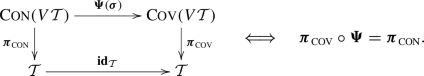 (183)
(183) -
2.
In turn, the symmetry condition:
$$\begin{aligned} {\langle }\hspace{1.00006pt}\textbf{H}(\varvec{\sigma })\cdot \delta _1\varvec{\sigma },\delta _2\varvec{\sigma }\hspace{1.00006pt}{\rangle } ={\langle }\hspace{1.00006pt}\textbf{H}(\varvec{\sigma })\cdot \delta _2\varvec{\sigma },\delta _1\varvec{\sigma }\hspace{1.00006pt}{\rangle }, \end{aligned}$$(184)ensures fiberwise integrability of the elastic response with a Green scalar elastic stress potential \(\,\Xi \,\)Footnote 26:
$$\begin{aligned} \varvec{\Psi }={d_{F}}\Xi , \quad \textbf{H}={d^2_{F}}\Xi . \end{aligned}$$(185)fulfilling the commutative diagram:
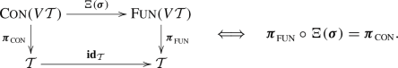 (186)
(186)


Time rates can be pulled-back to the initial configuration of the process and integrated to evaluate the corresponding finite increments.
Definition 3
(Elastic states) An elastic state \(\,\textbf{e}\textbf{s}\in {\textsc {Cov}}({T{\mathcal {C}}})\,\) is the symmetric twice covariant material tensor field on \(\,{\mathcal {C}}\,\) output of the (invertible) nonlinear constitutive relation:
The convective time rate of elastic state is equal to the elastic stretching [47]:
and the rate elastic law writes:
In this way, all involved fields are state variables.
Accordingly Hooke’s statement has to be modified into:
“vt vis mutat sic status elasticus”.
Covariance of the elastic compliance along the motion Eq. (180), integrability of the constitutive relation at any fixed time Eq. (185), and mass conservation Eq. (84) lead to assess no internal work is expended in a push-closed elastic process [45, 47, 49, 50, 72].
This essential characteristic feature of elastic models, is not achievable with the hypoelastic model proposed by Truesdell in [143], as proven by Barry Bernstein in [144].
In that regard, Rodney Hill observation in [145] was:
“ Truesdell ’s intention was to formulate a new concept of elastic behaviour or, more precisely, a concept of elastic behaviour expressed entirely in terms of rates. However, probably the overwhelming majority of hypo-elastic solids are inelastic”.
As a consequence of such a pessimistic sentiment, most scholars were induced to embrace the untenable proposal of a finite elasticity.
In the absence of other sources of deformation, the finite elastic strain was identified with the displacement gradient and the elastic power with the product of the Cauchy stress by the displacement gradient rate, a notion depending on the chosen connection or parallel transport:
not allowed in constitutive laws, according to the geometric paradigm [51].
In the rate theory of elasticity here developed, the internal elastic power per unit mass is expended by the natural stress in duality with the corresponding elastic stretching, both being state variables.
The integral of this internal elastic power in a time interval along the motion yields the relevant expended elastic work.
The implications of this new notion of elasticity are significant in all situations where nonlinearities play a decisive role.
As shown above, integrability entails existence of a stress potential but an elastic strain potential cannot be considered, contrary to usual statements.
Indeed, even when in pure elasticity, where the elastic stretching coincides with the geometric stretching, the strain is the difference in metric properties of the material at corresponding points of the body in two configurations at distinct time instants along the motion. Therefore the strain is not a state-variable pertaining to a single body configuration.
On the other hand, the basic feature of elasticity is that elastic stretching is induced by changes of stress state in the material.
This is the peculiar distinctive property with respect to other components of the total stretching induced by changes of internal microscopic structure of the material such as plastic, thermal, electric, magnetic fields and so on, occurring along the motion of the body.
The whole theory of material behaviour is based on considering the geometric stretching as the overall result of elastic, visco-plastic, thermal and electromagnetic stretching components whose addition is independent of any ordering.
The requirements of commutativity and associativity can only be fulfilled in a natural way in the context of a rate theory in which finite strains are replaced with their convective rate counterpart, the stretching fields.
According to Euler-Legendre-Fenchel transform, a complementary potential \(\,\Xi ^*(\textbf{e}\textbf{s})\,\) function of the elastic state, a novel notion stemming from integrability, is associated with a strictly convex George Green stress potential \(\,\Xi (\varvec{\sigma })\,\):
The nonlinear theory of elasticity currently displayed in articles and textbooks requires a proper reformulation from the very conceptual roots.
As a direct consequence of the rate theory, common treatments of elastic stability, based on the minimum properties of an alleged strain energy functional, dependent on the displacement field from some reference configuration, become void of physical content [70].
Denoting by a superimposed dot the Lie derivative of material fields along the motion, so that \(\,{\dot{\varvec{\sigma }}}=\mathcal {L}_{\textbf{V}_{\varvec{\varphi }}}(\varvec{\sigma })\,\) and \(\,\dot{\textbf{e}}\textbf{s}=\mathcal {L}_{\textbf{V}_{\varvec{\varphi }}}(\textbf{e}\textbf{s})\,\), Leibniz rule gives [72]:
From Euler-Legendre transform Eq. (191), we infer:
Summing up the two equalities in Eq. (192), from Eq. (193) we infer time rates of conjugate potentials sum to zero:
This result in Eq. (194) is purely mathematical regarding Euler-Legendre conjugate potentials on dual material tensor bundles on a nonlinear manifold, with no dependence upon constitutive assumptions.Footnote 27
In particular Eq. (194) proves invariance of the stress-state Green potential \(\,\Xi \,\) along the motion implies invariance of the elastic-state conjugate potential \(\,\Xi ^*\,\) and vice versa. The former is a characteristic assumption of elasticity theory and entails invariance along the motion of the elastic compliance operator \(\,\textbf{H}\,\).
16 Elasto-Thermo-Plasticity
Problems in Elasto-Thermo-Plasticity have longly been investigated, both from the theoretical and computational side.
Unfortunately, as commented above, around the middle of the past century a new proposal [147, 148] arose in an attempt to get a better matching with the nonlinear formulation of the Mechanics of Continua according to the treatment by Truesdell & Noll in [90].
The proposal, advanced by Erastus Henry Lee in [147, 148], was adopted by Juan Carlos Simó in [149] and still put over by Vlado Lubarda [150], with Robert J. Asaro in [151].
Nowadays the chain decomposition has spread over in literature with a completely undeserved success, as commented in the sequel.
The proposal was to split the deformation gradient as a chain of linear transformations acting pairwise between tangent spaces located at mysterious local configurations labeled as initial, intermediate and final (for elasto-plastic behaviour). The ordering of these local configurations in the chain was not motivated being left to the readers’ taste. More complex behaviours may involve also thermal, viscous and phase-change phenomena.
The indeterminacy of local configurations and of their ordering in the chain render the proposal conceptually unviable.
Also the physical meaning of the individual terms of the chain is definitely obscure and problematic, with the finite plastic strain giving rise to plastic stretching and plastic spin tensors.
Again, however, all these troubles were not sufficient to most knowledgeable people for giving up in perpetuating the mechanical crime over the years, as confirmed quite recently in [150, 151].
And yet, in the meanwhile, pioneering masters of computational mechanics were adopting, at the same epoch of the multiplicative chain proposal, a direct additive decomposition of the Euler stretching tensor (time-rate of change of the metric tensor) into a sum of constitutive components whose commutativity guarantees invariance under any permutation of ordering.
In fact, the insurmountable difficulties met by the chain proposal, are overcome by the rate model based on the notion of natural stress, as illustrated in § 15.1.
17 Rate equilibrium
A basic role in the nonlinear theory is played by the expression of the incremental virtual power principle, deduced from the instantaneous virtual power principle by time differentiation along the motion in the events spacetime.
In this differentiation the virtual velocity field on \(\,{\mathcal {C}}\,\) is extended to a Euclid spacetime field on the trajectory manifold by imposing invariance under parallel transport along the motion:
which amounts to fulfilling the differential condition:
The rate virtual power principle, appliying Leibniz rule of calculus, yields two additive terms.
The former consists of the incremental power performed by the stress time-rate along the motion in duality with the virtual stretching. The latter gives the incremental power performed by the stress in duality with the time-rate of the virtual stretching. This last term is the one responsible for possible lack of uniqueness or non-existence of solution of rate elasto-static problems, characteristic of instability phenomena [48, 71].
18 Electromagnetic induction
The basic geometric formula recalled in Eq. (25), appears to have not been appreciated as deserved in literature on continuum mechanics and electrodynamics.
Yet, its power could have prevented the persistence of long-standing incorrect formulations in dealing with the modelling of time-dependent physical phenomena.
A striking example of this powerfulness is offered in the field of Electrodynamics by the law of electric induction with the notion of Lorentz force acting on a moving electric charge crossing a uniform and constant magnetic vortex field.
In fact, the Lorentz force term is neither a force nor an invention of the Dutch physicist Hendrik Antoon Lorentz [85]. This notwithstanding the relevant formula is still so named and adopted by physicists worldwide.
Indeed, in the expression of the induced electric field Eq. (202), the single term involving the magnetic vortex two-form \(\,\varvec{\Omega }^2_\textbf{B}\in \Lambda ^2({{V\mathcal {T}}_\mathcal {E}})\,\):
being dependent on the spatial velocity \(\,\textbf{v}_{\varvec{\varphi }}=\textbf{P}{\textbf{V}_{\varvec{\varphi }}}\in {{V\mathcal {T}}_\mathcal {E}}\,\) of the point charge, does not fulfil Galileo Galilei relativity Principle 1.
Moreover, contrary to claims attributing the formula to H.A. Lorentz, the relevant expression was firstly conceived by James Clerk-Maxwell some forty year earlier as a partial additive term of a more general and fully covariant formulation of the magnetically induced electric field [82].
A careful investigation [52, 53, 68] shows the Lorentz force term stems out from an improper simplification consisting of merging the last velocity dependent term in Eq. (202) with the gradient of the electrostatic point potential.
The recent treatment [105] by Friedrich Wilhelm Hehl and Yuri Obukhov even assumes the Lorentz force term as a further axiom of Electrodynamics.
Richard Phillips Feynman [152] and Edward Mills Purcell [153], being aware of the dependence of the Lorentz force term on the observer measuring the involved spatial velocity, strove to justify the rule trying to bring into play the Special Theory of Relativity. The adopted proofs were however carried out according to what could be called a physicist’ way of doing.
In fact, the exposed proofs in [152] and [153] consist of a mixture of simple thought experiments and particular features concerning time and motion, measured by moving observers.
A direct application of the spacetime extrusion formula Eq. (26) led in a natural way to the mathematical expresssion of the induced electric field, as described below in Eq. (202).
The Michael Faraday [154] – Joseph Henry [155] electric induction law is usually expressed by physicists as a flux rule making reference to an outer orientation of the crossed surface.
The electromotive force is however expressed by the integral of the electric field along an inner oriented circuit and therefore the concatenated surface has to be likewise inner oriented.
The Faraday-Henry induction law should accordingly be more properly expressed as a vortex rule.
The circuital relation involves the electric field one-form \(\,\varvec{\Omega }^1_\textbf{E}\in \Lambda ^1({{V\mathcal {T}}_\mathcal {E}})\,\) and the magnetic vortex two-form \(\,\varvec{\Omega }^2_\textbf{B}\in \Lambda ^2({{V\mathcal {T}}_\mathcal {E}})\,\):
for any inner oriented spatial surface \(\,{S}_\textsc {inn}\,\).
The rule first formulated in 1834 by Emil Khristianovich Lenz [156] motivates the minus sign at the l.h.s. of Eq. (199).
The circuital vortex rule Eq. (199) is of limited usefulness in applications since most electric circuits are not boundaries of a surface. For solenoids the rule works effectively only in approximate computational schemes.
Moreover, for circuits undergoing irregular motions the vortex rule is not applicable and this explains the many claimed failures of the flux rule [152, 157].
Anyway, for regular motions of boundary circuits, the circuital law is meaningful because the integral at r.h.s. of Eq. (199) is independent of the choice of the surface \(\,{S}_\textsc {inn}\,\) having a given boundary circuit \(\,\partial {S}_\textsc {inn}\,\).
This independence is implied by absence of magnetic charges, expressed by the condition \(\,\texttt{d}\varvec{\Omega }^2_\textbf{B}=\textbf{0}\,\) which also assures existence of a magnetic potential \(\,\varvec{\Omega }^1_\textbf{B}\,\):
In regions with no magnetic charges, the circuital law in Eq. (199) can be effectively extended to a Faraday-Henry lineal law of electric induction.
The relevant statement is that, for inner oriented material lines \(\,L_\textsc {inn}\,\):
Localising, decomposing the velocity and applying the extrusion formula Eq. (26), the induced electric field is expressed by:
The first term at the r.h.s. of the last split in Eq. (202) is the partial time derivative of the magnetic momentum one-form \(\,\varvec{\Omega }^1_\textbf{B}\,\), and the second term is the so called Lorentz force.
These two terms are respectively referred to as transformer and motional components of the induced electric field in some books on applied Electrodynamics [158]. The third term is ignored at all.Footnote 28
Although the whole induction law Eq. (202) is covariant under Euclid transformations, no one of the three single terms at r.h.s. is such, not even with respect to Galilei transformations.
The so called Lorentz force rule:
for the motional component of the induced electric field consists of a simple expression in which the knowledge of the magnetic vortex and of the spatial velocity are only required at the point of evaluation.
This seemingly favourable feature deceptively appears to be extremely convenient for engineering applications and this could explain the formidable success of a dramatically unphysical formula.
The geometric analysis shows that Eq. (203) is equivalent to assume vanishing of the third, still motional term \(\,\texttt{d}(\varvec{\Omega }^1_\textbf{B}\cdot \textbf{P}{\textbf{V}_{\varvec{\varphi }}})\,\) in Eq. (202), a vanishing that can be easily ascertained not to hold as a rule.
The mathematical procedure here set into action leads however to recover in a modern key a particular statement made by Joseph John Thomson.
Indeed, in late years of nineteen century he provided in [160, p.534] a clarification of the expression given by his master James Clerk-Maxwell in [82].
The term \(\,\texttt{d}(\varvec{\Omega }^1_\textbf{B}\cdot \textbf{P}{\textbf{V}_{\varvec{\varphi }}})\,\) was correctly considered by Maxwell but, for simplicity sake, improperly merged with the gradient of the electrostatic potential, and therefore hidden to most readers.
Analogous results, without merging motional terms with static ones, were independently contributed by Hermann von Helmholtz [120].
These striking contributions were not adequately quoted in subsequent Physics and Engineering literature, see e.g. [161] where resort was rather made to the misleading simplifications introduced in \(\,1892\,\) by Rudolph Heinrich Hertz [162] and Oliver Heaviside [163], mainly interested in electric waves in vacuo, where no material movements are experienced [68].
As a matter of fact, Hertz warningFootnote 29 concerning the physical meaning of the single terms in the electric induction law was ignored by the Physics community and was likewise not quoted in Albert Einstein \(\,1905\,\) paper [86] entitled “On the Electrodynamics of moving bodies”.Footnote 30
There the author, contrary to what could be expected on reading the title, makes reference to electromagnetic induction phenomena in empty space. Indeed, the paper [86] begins with the doubtful words:
“It is known that Maxwell’s electrodynamics - as usually understood at the present time–when applied to moving bodies, leads to asymmetries which do not appear to be inherent in the phenomena.”
Lack of covariance of the electromagnetic induction law even under a simple Galilei change of frame is a direct consequence.
On the contrary, the spacetime geometric analysis outlined in § 19, leads to express the magnetically induced electric field with the spacetime Maxwell laws in Eqs. (209)–(217) which are covariant under any frame change in spacetime.
The physical inconsistency of the Lorentz force law has been anyway ignored by scholars in Electrodynamics.
In fact, Maugin in [102, 12.3.1], in commenting a theory conceived some forty years before with Eringen [164], declared the analysis to belong to “the most rewarding improvements brought to the electrodynamics of moving media in the 20th century”. On the other hand, he soon after declares the starting point for that analysis to be “the celebrated Lorentz force” [165].
18.1 Critical remarks on the Lorentz force
To the basic criticism expressed in § 18, we may add the further comment that the simplifications resulting from dropping the motional term \(\,\texttt{d}(\varvec{\Omega }^1_\textbf{B}\cdot \textbf{P}{\textbf{V}_{\varvec{\varphi }}})\,\) were even asserted by Olivier Darrigol [166] to be corrections of purportedly incorrect calculations of Joseph John Thomson [160], with no valid argument adduced.
The monograph Electric waves [162] by Hermann Hertz was wrongly credited by Darrigol [166] to have first proposed an ad hoc modification of electromagnetic induction laws to recover Galilei invariance.
Indeed, as quoted by Hertz himself in an apologising footnote [162, XIV, fn.2, p.247], the formulation of the induction law in terms of convective derivatives had been contributed, some thirty-seven years before, by Clerk-Maxwell in [82, Eq.(77), p.342].
The geometric analysis [42, 68] recovers for the force acting on an electric charge moving across a uniform field of magnetic vortices, the evaluation performed by J.J. Thomson [160].
The final result presents a correcting factor one half due to the last term in Eq. (202), which in that special case amounts to [52, 68]:
A positive answer is so given to the surrender of Feynman in [152, §17.1]:
“We know of no other place in physics where such a simple and accurate general principle requires for its real understanding an analysis in terms of two different phenomena.”
As a consequence of the geometrical analysis, also deprived of physical basis is the notion of Maxwell stress tensor which is derived from the untenable Lorentz force term.
19 Spacetime electromagnetic induction
A simplest awesome, although hermetic, formulation of the electric induction law in material bodies can be achieved by introducing on the spacetime trajectory \(\,{\mathcal {T}_\mathcal {E}}\,\) a Faraday two-form \(\,\varvec{\Omega }^2_{\textbf{F}}\in \Lambda ^2({T\mathcal {T}_\mathcal {E}})\,\) and a potential one-form \(\,\varvec{\Omega }^1_{\textbf{F}}\in \Lambda ^1({T\mathcal {T}_\mathcal {E}})\,\).
An innovative analysis [72] can then be performed by defining the projector:
and its complement \(\,\textbf{P}_{\varvec{\varphi }}:=\textbf{I}-\textbf{R}_{\varvec{\varphi }}\,\), in place of projectors \(\,\textbf{R}:=\varvec{\theta }\otimes \textbf{Z}:{T\mathcal {E}}\mapsto {T\mathcal {E}}\,\) and \(\,\textbf{P}:=\textbf{I}-\textbf{R}\,\) introduced in § , so that:
Accordingly, electric and magnetic time-vertical forms are given in terms of the two-form \(\,\varvec{\Omega }^2_{\textbf{F}}\in \Lambda ^2({T\mathcal {T}_\mathcal {E}})\,\) and of the potential one-form \(\,\varvec{\Omega }^1_{\textbf{F}}\in \Lambda ^1({T\mathcal {T}_\mathcal {E}})\,\) by:
with the splittings:
Closedness of Faraday two-form \(\,\varvec{\Omega }^2_{\textbf{F}}\in \Lambda ^2({T\mathcal {T}_\mathcal {E}})\,\) on the spacetime trajectory \(\,{\mathcal {T}_\mathcal {E}}\,\), is equivalent to the spatial system composed of Gauss law for the magnetic vortex and of Lenz-Faraday-Henry law of electric induction:
The spatial exterior derivative \(\,\texttt{d}_{S}\,\), acts on trajectory forms \(\,\varvec{\Omega }\in \Lambda ^k({T\mathcal {T}_\mathcal {E}})\,\) and is related to the spacetime exterior derivative \(\,\texttt{d}\,\) by:
The identity in Eq. (209) follows from the representation [72]:
where:
On the other hand, the induction laws of magnetic flux, involving time-vertical forms of electric flux, electric charge and electric current, are stated in the simplest manner in terms of the Ampère two-form \(\,\varvec{\Omega }^2_{\textbf{A}}\in \Lambda ^2({T\mathcal {T}_\mathcal {E}})\,\) and of the charge-current three-form \(\,\varvec{\Omega }^3_{\textbf{C}}\in \Lambda ^3({T\mathcal {T}_\mathcal {E}})\,\) on the spacetime trajectory \(\,{\mathcal {T}_\mathcal {E}}\,\), by setting:
with the splittings:
From Eq. (211) we get the representation:
with the last term trivially vanishing.
Hence, closedness of the charge-current three-form \(\,\varvec{\Omega }^3_{\textbf{C}}\in \Lambda ^3({T\mathcal {T}_\mathcal {E}})\,\) means balance of electric current and electric charge:
By Volterra theorem 1 the closedness condition Eq. (216) is equivalent to equality between the charge-current three-form \(\,\varvec{\Omega }^3_{\textbf{C}}\in \Lambda ^3({T\mathcal {T}_\mathcal {E}})\,\) and the exterior derivative of Ampère two-form \(\,\varvec{\Omega }^2_{\textbf{A}}\in \Lambda ^2({T\mathcal {T}_\mathcal {E}})\,\).
This is in turn equivalent to the time-vertical system composed of Gauss-Poisson law stating electric charges are sources for electric flux, and of Ampère-Maxwell magnetic induction law:
The electromagnetic induction laws, expressed by the spacetime formulations in Eqs. (209) and (217), are spacetime covariant under any frame change, thanks to commutativity of exterior derivative with push by a diffeomorphism [72].
The formulation of Maxwell equations in terms of the spacetime velocity \(\,{\textbf{V}_{\varvec{\varphi }}}:{\mathcal {T}_\mathcal {E}}\mapsto {T\mathcal {T}_\mathcal {E}}\,\) along the trajectory, as exposed in §. 19, a previously unpublished contribution of the first author, opens the way for dealing with electromagnetic fields in material bodies in a natural way.
Substitution of spacetime rigging field \(\,\textbf{Z}:\mathcal {E}\mapsto {T\mathcal {E}}\,\) with body velocity \(\,{\textbf{V}_{\varvec{\varphi }}}:{\mathcal {T}_\mathcal {E}}\mapsto {T\mathcal {T}_\mathcal {E}}\,\) along the trajectory, as made in Eqs. (207)–(208) and in Eqs. (213)–(214), is feasible since both fulfil the tuning property, see Eqs. (40) and (50).
Previous analyses [88, 126] of electromagnetic induction based on the split of the Faraday \(\,\varvec{\Omega }^2_{\textbf{F}}\in \Lambda ^2({T\mathcal {E}})\,\), the Ampère \(\,\varvec{\Omega }^2_{\textbf{A}}\in \Lambda ^2({T\mathcal {E}})\,\) and the charge-current \(\,\varvec{\Omega }^3_{\textbf{C}}\in \Lambda ^3({T\mathcal {E}})\,\) forms, have overlooked the fact that these tools where conceived for the empty spacetime with the rigging field \(\,\textbf{Z}:\mathcal {E}\mapsto {T\mathcal {E}}\,\) fixed by the observer.
In dealing with material bodies, motion must be taken into account. This task is accomplished in a natural way by replacing the above spacetime forms with the corresponding trajectory forms \(\,\varvec{\Omega }^2_{\textbf{F}}\in \Lambda ^2({T\mathcal {T}_\mathcal {E}})\,\), \(\,\varvec{\Omega }^2_{\textbf{A}}\in \Lambda ^2({T\mathcal {T}_\mathcal {E}})\,\) and \(\,\varvec{\Omega }^3_{\textbf{C}}\in \Lambda ^3({T\mathcal {T}_\mathcal {E}})\,\), which fulfil Eqs. (207) and (213), with the spacetime velocity field \(\,{\textbf{V}_{\varvec{\varphi }}}:\mathcal {E}\mapsto {T\mathcal {T}_\mathcal {E}}\,\) in place of the rigging field \(\,\textbf{Z}:\mathcal {E}\mapsto {T\mathcal {E}}\,\).
This slippage led to conceive the introduction of the Lorentz force rule as a deus ex machina ( ) dropped on the Electrodynamics stage.
The Lorentz force rule, being deceptively highly convenient in applications but deprived of physical content, is unveiled to be a poisoned gift offered to unwary mortals by a sneaky little devil.
20 Concluding remarks
Other notable achievements got by the geometric approach concern different items of Differential Geometry [46, 56], Thermodynamics [40], Propagation of singularities [72], Structured Continua [57], Nonlocal Elasticity [58,59,60, 63, 67], and Rate Electro-Magneto-Elasticity [72, 73].
Relevant analyses and results are collected and discussed in [72].
In conclusion of this long presentation, a sharp sentence by Bertrand Russell [167] (1919) is proposed as a warm invitation to dare a critical analysis also of so-called well-established theoretical constructs.
“ The fact that an opinion has been widely held is no evidence whatever that it is not utterly absurd; indeed in view of the silliness of the majority of mankind, a widespread belief is more likely to be foolish than sensible.”
This sentence was probably inspired by the Galileo Galilei vent in a letter to Johannes Kepler on August 19th 1610:
“ I think, my Kepler, we will laugh at the extraordinary stupidity of the multitude. What do you say to the leading philosophers of the faculty here, to whom I have offered a thousand times of my own accord to show my studies, but who with the lazy obstinacy of a serpent who has eaten his fill have never consented to look at planets, nor moon, nor telescope? Verily, just as serpents close their ears, so do these men close their eyes to the light of truth.”
These words do also agree with the comment of the Arab scientist Alhazen (see footnote 16) who around the turning of the first millennium stated:
“ If learning the truth is the scientis’s goal....then he must make himself the enemy of all that he reads.”
Experts in CME are thus called to improve knowledge of basic Differential Geometry and to take arms against a sea of troubles (Hamlet, Act III, Scene I [To be, or not to be]) to be faced in revising and correcting geometrically improper and physically unsustainable but still currently claimed notions and results, even located in the sancta sanctorum ( ) of knowledgeable people in CME.
Notes
Tensors at a point of a manifold are multilinear real valued functions whose arguments are vectors or covectors at that point of the manifold. Covariant tensors in \(\,{\textsc {Cov}}({T\mathcal {E}})\,\) have vector arguments in \(\,{T\mathcal {E}}\,\) while the arguments of contravariant ones in \(\,{\textsc {Con}}({T\mathcal {E}})\,\) are covectors in the dual bundle \(\,{({T\mathcal {E}})^*}\,\). Second order mixed tensors in \(\,{\textsc {Mix}}({T\mathcal {E}})\,\) have covector-vector pairs as arguments. Scalar functions in \(\,{\textsc {Fun}}({T\mathcal {E}})\,\) are zeroth order tensors.
Forms are alternating tensor fields.
The Hassler Whitney product \(\,{T\mathcal {M}}\times _\mathcal {M}{T\mathcal {M}}\,\) is made of pairs \(\,\{\textbf{u}_\textbf{x}\,,\textbf{v}_\textbf{x}\}\,\) with \(\,\textbf{x}\in \mathcal {M}\,\).
A.k.a. to Physicists as Osborne Reynolds transport formula: [114].
This simply says the boundary of the extruded tube is the chain composition of the back and front stoppers and of the lateral mantle, with the appropriate signs.
Fiber differentials \(\,{d_{F}}\,\) are taken while holding the basic point fixed.
As customary, a superscript \(\,*\,\) denotes duality.
A submersion is a map with a surjective differential at any point. \(\,\mathcal {Z}\,\) is initial of the German word Zeit meaning time.
Empty here means massless.
Named after the Norwegian geometer Marius Sophus Lie, by David van Dantzig [113] (Liesche ableitung).
The inclusion \(\,\textbf{i}_{\mathcal {E}}:\mathcal {T}\mapsto \mathcal {E}\,\) is an immersion if \(\,T\textbf{i}_{\mathcal {E}}:{T\mathcal {T}}\mapsto {T\mathcal {E}}\,\) is pointwise injective.
First enunciated by Johann Bernoulli as far as 1717 in a letter to Pierre Varignon.
Alhazen latinisation of al-Hasan, was the author of the 7-vols. Kitab al Manazir (Book of Optics) (1011 to 1021) and is known as Father of Optics.
Duly extended, according to our observations, by push-forward along each virtual flow.
In the dual \(\,\mathcal {X}^*\,\) of a linear space \(\,\mathcal {X}\,\), the polar: of a linear subspace \(\,\mathcal {L}\subset \mathcal {X}\,\) is the subspace \(\,\mathcal {L}^\circ \subset \mathcal {X}^*\,\) defined as \(\,\mathcal {L}^\circ :=\{\textbf{u}^*\in \mathcal {X}^*\mid {\langle }\hspace{1.00006pt}\textbf{u}^*,\textbf{u}\hspace{1.00006pt}{\rangle }=0\quad \forall \,\textbf{u}\in \mathcal {L}\}\,\).
Immersions (surjections) have injective (surjective) tangent maps at any point.
The projections \(\,\varvec{\pi }_\textsc {con}\,\) and \(\,\varvec{\pi }_\textsc {cov}\,\) map the stress and stretching tensors onto their base point in the spacetime trajectory \(\,\mathcal {T}\,\), and define the stress and stretching bundles.
Eq. (194) is formally analogous to, but more general than, the one exposed by Rodney Hill and James Robert (Jim) Rice in [146, Eq.(13)] where the conjugate potentials defining ultra-elastic constitutive relations were dealt with in terms of strains measured from a reference placement to the actual one.
An instance is Eq.(8) in [159].
In [162, XVI-2, p.248] Heinrich RudolfHertz statement about Lorentz force was: “Now the resultant of \(\,(X_1,X_2,X_3)\,\) is an electric force which arises as soon as a body moves in the magnetic field. It is that force which in a narrower sense we are accustomed to denote as the electromotive force induced through the motion. But it should be observed that, according to our views, the separation of this from the total force can have no physical meaning.”
But, are there non-moving bodies, independently of the observer?
 means image.
References
Romano, G.: Limiti di collasso rigido plastico di piastre rettangolari soggette a carichi simmetrici rispetto alle mediane. Ingegneria Civile 30, 1–19 (1969)
Romano, G.: Potential operators and conservative systems. Meccanica 7(3), 141–146 (1972). https://doi.org/10.1007/BF02128759
Romano, G.: On the minimum of the potential energy functional at a critical point. Meccanica 9(4), 198–202 (1974). https://doi.org/10.1007/BF02175805
Romano, G.: On the energy criterion for the stability of continuous elastic structures. Meccanica 10(3), 198–202 (1975). https://doi.org/10.1007/BF02149034
Romano, G.: Postcritical behaviour of elastic structures: part I: incremental uniqueness and stability. University of Calabria Department of Structures, Report (8 April 1975). http://wpage.unina.it/romano/selected-publications/
Romano, G.: Postcritical behaviour of elastic structures: part II: postcritical analysis and imperfection sensitivity. University of Calabria Department of Structures, Report (9 April 1975). http://wpage.unina.it/romano/selected-publications/
Romano, G., Romano, M.: Sulla soluzione di problemi strutturali in presenza di legami costitutivi unilaterali. Acc. Naz. Lincei; Rend. Sc. Fis. Mat. Nat., Serie VIII, vol. LXVII, fasc. 1–2, Ferie (1979). http://wpage.unina.it/romano/selected-publications/
Romano, G.: Duality and variational principles in structural mechanics under bilateral and unilateral constraints. Laboratorio de Computaçao Cientifica (L.C.C.) CNPq, Rio de Janeiro, Brazil (1982)
Romano, G., Romano, M.: Elastostatics of structures with unilateral conditions on stress and displacements fields. In: CISM Courses and Lectures, vol. 288, pp. 315–338. Springer, New York-Wien (1985)
Romano, G., Rosati, L.: Variational Principles in Convex Structural Analysis, Volume in Onore del Prof. Giulio Ceradini, Roma (1988)
Romano, G., Rosati, L.: On Limit States, Plasticity and Locking. IX Congresso Naz. AIMETA, Bari (4–7 October 1988)
Romano, G., Rosati, L.: A Survey on Recent Advances in Convex Structural Analysis. Meccanica dei Materiali e delle Strutture, Atti del Convegno Nazionale in ricordo di Riccardo Baldacci e Michele Capurso, Roma (25–27 October 1989)
Romano, G., Rosati, L., Marotti de Sciarra, F.: An internal variable theory of inelastic behaviour derived from the uniaxial rigid-perfectly plastic law. Int. J. Eng. Sci. 31(8), 1105–1120 (1992)
Romano, G., Rosati, L., Marotti de Sciarra, F.: Variational principles for a class of finite-step elasto-plastic problems with non-linear mixed hardening. Comput. Methods Appl. Mech. Eng. 109, 293–314 (1993)
Romano, G., Rosati, L., Marotti de Sciarra, F.: A variational theory for finite-step elasto-plastic problems. Int. J. Solids Struct. 30(17), 2317–2334 (1993)
Romano, G., Rosati, L., Marotti de Sciarra, F., Bisegna, P.: A potential theory for monotone multi-valued operators. Q. Appl. Math. 51(4), 613–631 (1993)
Romano, G., Rosati, L., Marotti de Sciarra, F.: Variational formulations of non-linear and non-smooth structural problems. Int. J. Non-linear Mech. 28, 195–208 (1993)
Romano, G., Rosati, L., Marotti de Sciarra, F.: A variational theory for finite-step elasto-plastic problems, Letter to the editor. Int. J. Solids Struct. 32(10), 1477–1478 (1995)
Romano, G., Rosati, L., Marotti de Sciarra, F.: A variational theory for finite-step elasto-plastic problems. Authors closure. Int. J. Solids Struct. 32(10), 1479–1480 (1995)
Romano, G.: New results in subdifferential calculus with applications to convex optimization. Appl. Math. Optim. 32, 213–234 (1995)
Romano, G., Marotti de Sciarra, F., Diaco, M.: Mixed Formulation, Localization and LBB condition. Proceedings SACAM ’98 University of Cape Town, South Africa (1998)
Romano, G., Rosati, L., Diaco, M.: Well-posedness of mixed formulations in elasticity. ZAMM 79(7), 435–454 (1999)
Romano, G.: On the necessity of Korn’s inequality. In: O’ Donoghue P.E., Flavin J.N. (Eds) Trends in Applications of Mathematics to Mechanics, pp. 166–173. Elsevier, Paris. ISBN: 2-84299-245-8 (2000). http://wpage.unina.it/romano/selected-publications
Romano, G.: Theory of Structures, Part I, Elements of Linear Analysis. Lecture notes, University of Naples Federico II, Naples, Italy. http://wpage.unina.it/romano/selected-publications/(in Italian) (2000)
Romano, G., Diaco, M.: The strain gap method existence, uniqueness and convergence properties. In: Proceedings of Symposium on Trends in Application of Mathematics to Mechanics, STAMM2000, pp. 172–177. Elsevier, Paris (2000). http://wpage.unina.it/romano/selected-publications/
Romano, G., Marotti de Sciarra, F., Diaco, M.: Well-posedness and numerical performances of the strain gap method. Int. J. Num. Methods Eng. 51, 283–306 (2001)
Romano, G.: Scienza delle Costruzioni, Tomo Zero: Premesse matematiche. http://wpage.unina.it/romano/selected-publications/(in Italian) (2001)
Romano, G.: Scienza delle Costruzioni, Tomo I: Cinematica ed Equilibrio. http://wpage.unina.it/romano/selected-publications/(in Italian) (2002)
Romano, G.: Scienza delle Costruzioni, Tomo II: Elasticità e Resistenza. http://wpage.unina.it/romano/selected-publications/(in Italian)(2002)
Romano, G., Diaco, M.: A functional framework for applied continuum mechanics. In: New Trends in Mathematical Physics. World Scientific, Singapore, pp. 193–204 (2004). http://wpage.unina.it/romano/selected-publications/
Romano, G., Barretta, R., Sellitto, C.: On the evaluation of the elastoplastic tangent stiffness. In: Owen, D.R.J., Onate, E., Suarez, B. (Eds.) Computational Plasticity—Fundamentals and Applications, Part 2, CIMNE, Barcelona, pp. 1118–1121. ISBN: 84-95999-79-X (2005). http://wpage.unina.it/romano/selected-publications/
Romano, G., Diaco, M., Barretta, R.: On the theory of material inhomogeneities. Mech. Res. Commun. 33(6), 758–763 (2006)
Romano, G., Diaco, M., Barretta, R.: Basic issues in phase transition theory and fracture mechanics. In: Taroco E., de Souza Neto E.A., Novotny A.A. (Eds.) Variational Formulations in Mechanics: Theory and Applications, CIMNE, Barcelona, pp. 263-279, ISBN: 978-84-96736-32-0 (2007). http://wpage.unina.it/romano/selected-publications/
Romano, G., Sellitto, C., Barretta, R.: Nonlinear shell theory: a duality approach. J. Mech. Mater. Struct. 2(7), 1207–1230 (2007)
Romano, G., Barretta, R.: Cosserat Materials? No, thanks. Meeting of the Material Group of AIMETA (GMA), Genova, Italy (29 February–1 March 2008). http://wpage.unina.it/romano/lecture-slides/
Romano, G., Barretta, R., Diaco, M.: On the general form of the law of dynamics. Int. J. Non-linear Mech. 44(6), 689–695 (2009)
Romano, G., Barretta, R., Diaco, M.: On continuum dynamics. J. Math. Phys. 50(102903), 1–26 (2009)
Romano, G., Barretta, R., Barretta, A.: On Maupertuis principle in dynamics. Rep. Math. Phys. 63(3), 331–346 (2009)
Romano, G., Barretta, R., Diaco, M.: Algorithmic tangent stiffness in elastoplasticity and elastoviscoplasticity: a geometric insight. Mech. Res. Commun. 37(6), 289–292 (2010)
Romano, G., Diaco, M., Barretta, R.: Variational formulation of the first principle of continuum thermodynamics. Contin. Mech. Thermodyn. 22(3), 177–187 (2010)
Romano, G., Barretta, R.: Covariant hypo-elasticity. Eur. J. Mech. A/Solids 30(6), 1012–1023 (2011)
Romano, G.: On the laws of electromagnetic induction. arXiv: 1105.3340. IOP on-line, pp. 1–67 (2012). arXiv:1105.3340pdf
Romano, G.: Geometria della Deformazione. http://wpage.unina.it/romano/lecture-notes/(In Italian) (2012)
Romano, G., Barretta, R.: On Euler’s stretching formula in continuum mechanics. Acta Mech. 224, 211–230 (2013)
Romano, G., Barretta, R.: Geometric constitutive theory and frame invariance. Int. J. Non-linear Mech. 51, 75–86 (2013)
Romano, G.: On natural derivatives and the curvature formula in fiber bundles. Rend. Acc. Naz. Sc. Let. Arti, Napoli (2014). arXiv:1107.1705 [math.DG]
Romano, G., Barretta, R., Diaco, M.: The geometry of nonlinear elasticity. Acta Mech. 225(11), 3199–3235 (2014)
Romano, G., Barretta, R., Diaco, M.: Rate formulations in nonlinear continuum mechanics. Acta Mech. 225(6), 1625–1648 (2014)
Romano, G.: Geometry & Continuum Mechanics. Ed. CreateSpace Independent Publishing Platform (10 November 2014)
Romano, G.: Geometry & Continuum Mechanics. Short Course in Innsbruck, 24–25 November 2014. ISBN-10: 1503172198. http://wpage.unina.it/romano/lecture-slides/
Romano, G., Barretta, R., Diaco, M.: Geometric continuum mechanics. Meccanica 49(1), 111–133 (2014)
Romano, G.: Beyond Feynman’s troubles in electromagnetics. Rend. Acc. Naz. Sc. Let. Arti, in Napoli (2014). http://wpage.unina.it/romano/selected-publications/
Romano, G.: On time and length in special relativity. Rend. Acc. Naz. Sc. Let. Arti, Napoli (2014). http://wpage.unina.it/romano/selected-publications/
Romano, G., Barretta, R., Diaco, M.: Geometric action principles in classical dynamics. Rend. Acc. Naz. Sc. Let. Arti, Napoli (2015). http://wpage.unina.it/romano/selected-publications/
Romano, G.: Continuum mechanics and electrodynamics on manifolds (2015). Downloadable from http://wpage.unina.it/romano/selected-publications/
Romano, G.: Elements of differential geometry (2015). Downloadable from http://wpage.unina.it/romano/selected-publications/
Romano, G., Barretta, R., Diaco, M.: Micromorphic continua: non-redundant formulations. Contin. Mech. Thermodyn. 28(6), 1659–1670 (2016)
Romano, G., Barretta, R., Diaco, M., Marotti de Sciarra, F.: Constitutive boundary conditions and paradoxes in nonlocal elastic nanobeams. Int. J. Mech. Sci. 121, 151–156 (2017)
Romano, G., Barretta, R.: Stress-driven versus strain-driven nonlocal integral model for elastic nano-beams. Compos. Part B: Eng. 114, 184–188 (2017)
Romano, G., Barretta, R.: Nonlocal elasticity in nanobeams: the stress-driven integral model. Int. J. Eng. Sci. 115, 14–27 (2017)
Romano, G., Barretta, R., Diaco, M.: On nonlocal integral models for elastic nano-beams. Int. J. Mech. Sci. 131–132, 490–499 (2017)
Romano, G., Barretta, R., Diaco, M.: Solid-Fluid interaction: a continuum mechanics assessment. Acta Mech. 228, 851–869 (2017)
Romano, G., Luciano, R., Barretta, R., Diaco, M.: Nonlocal integral elasticity in nanostructures, mixtures, boundary effects and limit behaviours. Contin. Mech. Thermodyn. 30, 641–655 (2018)
Romano, G., Barretta, R., Diaco, M.: On the role of control windows in continuum dynamics. Acta Mech. 229, 1849–1868 (2018)
Romano, G., Barretta, R., Diaco, M.: The notion of elastic state and application to nonlocal models. In: Proceedings AIMETA 2017, vol. III, pp. 1156–1167 (2018)
Romano, G., Barretta, R., Diaco, M.: A geometric rationale for objectivity, stress rate, covariance and invariance. Contin. Mech. Thermodyn. 30, 175–194 (2018)
Romano, G., Barretta, R., Diaco, M.: Iterative methods for nonlocal elasticity problems. Contin. Mech. Thermodyn. 31, 669–689 (2019)
Romano, G.: Electrodynamics without Lorentz force (2021). arXiv:1209.5960v3
Romano, G., Diaco, M.: On formulation of nonlocal elasticity problems. Meccanica 56, 1303–1328 (2021)
Romano, G., Barretta, R., Diaco, M.: Genesis and progress of virtual power principle. Acta Mech. 233, 5431–5445 (2022)
Romano, G., Barretta, R., Diaco, M.: Spacetime evolutive equilibrium in non-linear continuum mechanics. Contin. Mech. Thermodyn. 30, 1859–1880 (2023)
Romano, G.: Continuum Mechanics and Electrodynamics: Geometric Foundations (2023). About 1800 pages (in completion) posted in https://gioprof1941.web.app
Romano, G., Barretta, R.: Non-Linear Electro-Magneto-Elasticity. In construction (2024)
Romano, M.: Scritti Scelti di Manfredi Romano. Istituto di Scienza delle Costruzioni, Universitá di Catania (1990). https://gioprof1941.web.app
Galilei, G.: Dialogo di Galileo Galilei Linceo Matematico Sopraordinario dello studio di Pisa. E Filosofo e Matematico primario del serenissimo GR. Duca di Tofcana. Doue nei congreffi di quattro giornate si difcorre fopra i due Massimi Sistemi del Mondo Tolemaico, e Copernicano; Proponendo indeterminatamente le ragioni Filosofiche, e Naturali tanto per l’una quanto per l’altra parte. In Fiorenza per GiovanBatifta Landini m.d.c.xxxii (1632)
Galilei, G.: Discorsi e Dimostrazioni Matematiche intorno a due nuove Scienze Attenenti alla Mecanica e & i Movimenti Locali, del signor Galileo Galilei Linceo, Filosofo e Matematico primario del Sereniffimo Gran Duca di Tofcana. Con una Appendice del centro di gravità d’alcuni solidi. Leida, Appreffo gli Elfevirii m.d.c.xxxviii (1638)
Newton, I.: Philosophiae naturalis principia mathematica. Typis Jofephi Streater, London (1687). English traslation by A. Motte (1729). The Principia, Mathematical Principles of Natural Philosophy. Isaac Newton (Author), I. Bernard Cohen, Anne Whitman, Julia Budenz (Translators) University of California Press (1999)
Leibniz, G.W. von: Die Leibniz-Handschriften der Königlichen öffentlichen Bibliothek zu Hannover (1895). http://www.gottfried-wilhelm-leibniz-gesellschaft.de/leibniz-digital-resources/3-handschriften.html
d’Alembert J-B. Le Ronde.: Traité de Dynamique. J-B. Coignard, Paris (1743)
Euler, L.: Methodus inveniendi lineas curvas maximi minimive proprietate gaudentes, sive solutio problematis isoperimetrici latissimo sensu accepti, additamentum II. Marcum Michaelem Bosquet, Lausanne (1744). Opera Omnia, Caratheodory C. (Ed.), LII-LV, pp. 298–308. Fussli, Zürich, Switzerland (1952)
Euler, L.: Decouvert d’un nouveau principe de la mécanique. Euler’s Opera Omnia II 5, pp. 81-108 (1750). Presented to the Berlin Academy in 3 Sep 1950 and originally published in Memoires de l’Acadėmie des Sciences de Berlin 6, 1752, pp. 185–217
Clerk-Maxwell, J.: On Faraday’s lines of force, Transactions of the Cambridge Philosophical, vol. X, Part I (Dec. 10, 1855 and Feb. 11, 1856)
Clerk-Maxwell, J.: On Physical Lines of Force, The London, Edinburgh, Dublin Phil. Mag. and J. Sci., Fourth series, Part I, II, III, IV.s (1861)
Clerk-Maxwell, J.: A Treatise on Electricity and Magnetism, vol. I. Oxford at Clarendon Press, II (1873)
Lorentz, H.A.: Versuch einer Theorie der electrischen und optischen Erscheinungen in bewegten Körpern. E. J. Brill, Leiden (1895)
Einstein, A.: Zur Elektrodynamik bewegter Körper. Annalen der Physik 17, 891 (1905). English transl. On the Electrodynamics of moving bodies. http://hermes.ffn.ub.es/luisnavarro/nuevo_maletin/Einstein_1905_relativity.pdf
Weyl, H.: Raum-Zeit-Materie. Springer, Berlin (1922). Temps-Espace-Matiére. Blanchard, Paris (1922). Space-Time-Matter. Dover, New York (1950)
Misner, C.W., Thorne, K.S., Wheeler, J.A.: Gravitation. W.H. Freeman, San Francisco (1973)
Truesdell, C.A., Toupin, R.: The Classical Field Theories, Handbuck der Physik, Ed. by Siegfried Flügge, band III/1, Springer-Verlag, Berlin, 226-793 (1960)
Truesdell, C.A., Noll, W.: The Non-Linear Field Theories of Mechanics. Handbuch der Physik, Siegfried Flügge (1965), 2nd edn. (1992), 3rd Ed. S. Antman (2004), Springer, New York
Gurtin, M.E.: The Linear Theory of Elasticity. Flügge, Siegfried; Truesdell, Clifford A. (eds.), Festerkorpermechanik/Mechanics of Solids, Handbuch der Physik VI/a. Springer, Berlin (1972)
Gurtin, M.E.: An Introduction to Continuum Mechanics. Academic Press, San Diego (1981)
Gurtin, M.E.: Topics in Finite Elasticity. Hamilton Press, Berlin, SIAM, Philadelphia, PA (1983)
Fichera, G.: Existence Theorems in Elasticity. Vol.VI/a, Springer-Verlag, Berlin, Handbuch der Physik (1972)
Fichera, G.: Boundary Value Problems of Elasticity with Unilateral Constraints. Handbuch der Physik, vol. VI/a. Springer-Verlag, Berlin (1972)
Arnol’d, V.I.: Matematicheskie metody klassicheskoi mekhaniki, Nauka, Moscow. (Mathematical methods of classical mechanics) (1974). English transl. by A. Weinstein and K. Vogtmann. Springer-Verlag, New York (1978-1989)
Abraham, R.H.: Foundations of Mechanics. Benjamin/Cummings, Reading Massachusetts (1967)
Abraham, R.H., Marsden, J.E.: Foundations of Mechanics. Benjamin, Reading Massachusetts (1978)
Abraham, R.H., Marsden, J.E., Ratiu, T.: Manifolds, Tensor Analysis, and Applications. Addison-Wesley, 2nd edn. (1988), 3rd edn (2003). Springer Verlag, New York (1983)
Marsden, J.E., Hughes, T.J.R.: Mathematical Foundations of Elasticity. Prentice-Hall, Redwood City, Cal (1983)
Podio-Guidugli, P.: A primer in elasticity. J. Elast. 58(1), 1–104 (2000)
Maugin, G.A. Continuum Mechanics Through the Twentieth Century. A Concise Historical Perspective. Solid Mechanics and Its Applications, vol. 196. Springer (2013)
Eringen, A.C., Maugin, G.A.: Electrodynamics of Continua I: Foundations and Solid Media. Springer, (1990)
Eringen, A.C., Maugin, G.A.: Electrodynamics of Continua II: Fluids and Complex Media. Springer (1990)
Hehl, F.W., Obukhov, Yu.N.: Foundations of Classical Electrodynamics, Charge, Flux and Metric. Birkhäuser, Boston (2003)
Minkowski, H.: Raum und Zeit. Lecture given at the 80th Meeting of Natural Scientists in Cologne on 21 September 1908. Phys. Z. 10, 75–88 (1908)
Spivak, M.D.: A comprehensive Introduction to Differential Geometry (1970). Vol.I-V, 3rd edn. rev. Publish or Perish, Inc., Houston (1979,1999)
Kolar, I., Michor, P.W., Slovak, J.: Natural Operations in Differential Geometry. Springer-Verlag, Berlin (1993)
Hitchin, N.: Differentiable Manifolds (2003). https://www1.mat.uniroma1.it/people/manetti/GeoDiff0809/HitchinDiff.pdf
Bossavit, A.: On the geometry of electromagnetism, Lecture 1–10. J. Jpn. Soc. Appl. Electromagn. Mech. 6, 17–28 (1998)
Veblen, O., Whitehead, J.H.C.: The Foundations of Differential Geometry. Cambridge Tracts 29, Cambridge University Press (1932)
Schouten, J.A.: Tensor Analysis for Physicists. Oxford University Press, London (1951). Dover, New York (1989)
van Dantzig, D.: On the geometrical representation of elementary physical objects and the relations between geometry and physics. Nieuw. Archief vor Wiskunde 3(2), 73–89 (1954)
Reynolds, O.: Papers on Mechanical and Physical Subjects. 3 12–13, The Sub-Mechanics of the Universe. Cambridge University Press (1903)
Samelson, H.: Differential forms, the early days; or the stories of Deahna’s theorem and of Volterra’s theorem. Am. Math. Mon. 108(6), 522–530 (2001)
Volterra, V.: Delle variabili complesse negli iperspazii, Rend. Accad. dei Lincei, ser. IV, vol. V, Nota I, 158-165, Nota II, 291-299 (1889) = Opere Matematiche, Accad. Nazionale dei Lincei, Roma 1, 403-410, 411–419 (1954)
Volterra, V.: Sulle funzioni conjugate, Rend. Accad. dei Lincei, ser. IV, vol. V, 599-611 (1889) = Opere Matematiche, Accad. Nazionale dei Lincei, Roma 1, 420–432 (1954)
Fubini, G.: Sugli integrali multipli. Rend. Acc. Naz. Lincei, classe di scienze fisiche, mat. e natur., XVII, pp. 608–614 (1907)
Tonelli, L.: Sull’integrazione per parti. Atti Accademia Nazionale dei Lincei 18(2), 246–253 (1909)
Helmholtz, H. von.: Über die Theorie der Elektrodynamik. Dritte Abhandlung: Die Elektrodynamischen Kräfte in bewegten Leitern. Journal für die reine und angewandte Mathematik (1874)
Trautman, A.: Remarks on the history of the notion of Lie differentiation. In: Krupková, O., Saunders, D.J. (eds.) Variations, Geometry and Physics. Nova Science Publishers (2008)
Cartan, É.: Leçons sur les Invariants Intégraux. Hermann, Paris (1922)
Poincaré, H.: Sur une forme nouvelle des équations de la méchanique. C. R. Acad. Sci. 132, 369–371 (1901)
Palais, R.S.: Definition of the exterior derivative in terms of the Lie derivative. Proc. Am. Math. Soc. 5, 902–908 (1954)
Friedman, M.: Foundations of Space-Time Theories. Princeton University Press (1983)
Fecko, M.: On 3+1 decompositions with respect to an observer field via differential forms. J. Math. Phys. 38, 4542–4560 (1997)
Deahna, F.: Ueber die Bedingungen der Integrabilität linearer Differentialgleichungen erster Ordnung zwischen einer beliebigen Anzahl veränderlicher Größen. J. für die Reine Angew. Math. 20, 340–350 (1840)
Frobenius, G.: Über das Pfaffsche Problem. J. Reine Angew. Math. 82 230–315 (1875) = Gesammelte Abhandlungen, Springer-Verlag Berlin (1966)
Panicaud, B., Rouhaud, E., Altmeyer, G., Wang, M., Kerner, R., Roos, A., Ameline, O.: Consistent hypo-elastic behavior using the four-dimensional formalism of differential geometry. Acta Mech. 227, 651–675 (2016)
Piola, G.: La meccanica dei corpi naturalmente estesi trattata col calcolo delle variazioni. Opusc. Mat. Fis. di Diversi Autori, Giusti, Milano 2, 201–236 (1833)
Kirchhoff, G.R.: Über die Gleichungen des Gleichgewichts eines elastischen Korpers bei nicht unendlich kleinen Verschiebungen seiner Theile. Akad. Wiss. Wien 9, 762–773 (1852)
Bertrand, J.: Mémoire sur l’integration des équations différentielles de la Mécanique. Liouville’s J. 17, 393–436 (1852)
Lagrange, J.-L.: Mécanique Analytique. Nouvelle Édition revue et augmentée par l’auteur, 2 vols, Veuve Courcier, Paris (1811)
Hamilton, W.R.: On a general method in dynamics. Philos. Trans. R. Soc. Part II, 247–308 (1834)
Hamilton, W.R.: Second essay on a general method in dynamics. Philos. Trans. R. Soc. Part I(125), 95–144 (1835)
Arnol’d, V.I., Kozlov, V.V., Neishtadt, A.I.: Dynamical Systems, III, Encyclopaedia of Mathematical Sciences. In: Arnol’d V.I. (Ed.), Springer-Verlag, New York, Berlin (1988)
Ogborn, J., Hanc, J., Taylor, E.F.: Action on stage: historical introduction. In: The GIREP Conference 2006, Modeling in Physics and Physics Education, Universiteit van Amsterdam (2006). https://www.eftaylor.com/pub/ActionSummary.pdf
Taylor, E.F.: Principle of Least Action. MIT (2008). http://www.eftaylor.com/leastaction.html
Goldstein, H.: Classical Mechanics. Addison Wesley, Reading, Mass (1950)
Yosida, K.: Functional Analysis. Springer-Verlag, New York (1980)
Hamilton, W.R.: On a general Method of expressing the Paths of Light, and of the Planets, by the Coefficients of a Characteristic Function. Dublin University Review and Quarterly Magazine 1, 795–826 (1833)
Green, G.: On the propagation of light in crystallised media. Trans. Camb. Philos. Soc. 7(1), 121–140 (1839)
Truesdell, C.A.: Hypo-elasticity. J. Ration. Mech. Anal. 4(83–133), 1019–1020 (1955)
Bernstein, B.: Hypo-elasticity and elasticity. Arch. Ration. Mech. Anal. 6(1960), 90–104 (1960)
Hill, R.: Some basic principles in the mechanics of solids without a natural time. J. Mech. Phys. Solids 7, 200–225 (1959)
Hill, R., Rice, J.R.: Elastic potentials and the structure of inelastic constitutive laws. SIAM J. Appl. Math. 25, 448–461 (1973)
Lee, E.H., Liu, D.T.: Finite strain elastic-plastic theory particularly for plane wave analysis. J. Appl. Phys. 38, 19–27 (1967)
Lee, E.H.: Elastic-plastic deformations at finite strains. ASME Trans. J. Appl. Mech. 36, 1–6 (1969)
Simó, J.C.: A framework for finite strain elastoplasticity based on maximum plastic dissipation and the multiplicative decomposition: continuum formulation. Comput. Methods Appl. Mech. Eng. 66, 199–219 (1988)
Lubarda, V.A.: Constitutive theories based on the multiplicative decomposition deformation gradient: thermoelasticity, elastoplasticity, and biomechanics. Appl. Mech. Rev. 57, 95–108 (2004)
Asaro, R., Lubarda, V.: Mechanics of Solids and Materials. Cambridge University Press (2006)
Feynman, R.P., Leighton, R.B., Sands, M.L.: The Feynman Lectures on Physics. Pearson/Addison-Wesley, San Francisco (1964)
Purcell, E.M.: Berkeley Physics Course, vol. 2. McGraw-Hill, NY (1965)
Faraday, M.: Experimental Reseaches in Electricity. Phil. Trans, London (1838)
Henry, J.: Scientific Writings of Joseph Henry. Smithsonian Institution, Washington (1886)
Lenz, E.: Über die Bestimmung der Richtung durch elektrodyanamische Vertheilung erregten galvanischen Ströme. Annalen der Physik und Chemie 31, 483 (1834)
Munley, F.: Challenges to Faraday’s flux rule. Am. J. Phys. 72(12), 1478 (2004). https://doi.org/10.1119/1.1789163
Sadiku, M.N.O.: Elements of Electromagnetics. Oxford University Press, USA (2010)
Corson, D.R.: Electromagnetic induction in moving systems. Am. J. Phys. 24, 126–130 (1955)
Thomson, J.J.: Notes on recent researches in electricity and magnetism, intended as a sequel to Professor Clerk-Maxwell’s ’Treatise on Electricity and Magnetism. Macmillan and Co. London (1893). https://archive.org/details/notesonrecentre01thomgoog
Jackson, J.D.: Classical Electrodynamics, 3rd edn. Wiley, New York (1999)
Hertz, H.R.: Untersuchungen über die Ausbreitung der Electrischen Kraft. Teubner, Leipzig. Investigations into the propagation of electrical force (1892). Dover, NY, 1962. http://ebooks.library.cornell.edu/c/cdl/
Heaviside, O.: Electrical Papers, vol. I, II. Macmillan & Co., London (1892)
Maugin, G.A., Eringen, A.C.: On the equations of the electrodynamics of deformable bodies of finite extent. J. Mécanique 16, 1–47 (1977)
Lorentz, H.A.: Theory of electrons. Teubner, Leipzig (1909) [Reprint, Dover, New York (1952)]
Darrigol, O.: Electrodynamics from Ampère to Einstein. Oxford University Press (2000)
Russell, B.: Introduction to mathematical philosophy (1919). Repr. in 1993 by Dover Publications, New York
Acknowledgements
Financial support from the Italian Ministry of University and Research (MUR) in the framework of the Project PRIN - code 2022ZW2NMJ - Nonlocal Mechanics of Innovative Soft Nanostructures (NoMISN), is gratefully acknowledged.

Funding
Open access funding provided by Università degli Studi di Napoli Federico II within the CRUI-CARE Agreement.
Author information
Authors and Affiliations
Corresponding author
Ethics declarations
Conflict of interest
The authors have no relevant financial or non-financial interests to disclose.
Additional information
Publisher's Note
Springer Nature remains neutral with regard to jurisdictional claims in published maps and institutional affiliations.
Rights and permissions
Open Access This article is licensed under a Creative Commons Attribution 4.0 International License, which permits use, sharing, adaptation, distribution and reproduction in any medium or format, as long as you give appropriate credit to the original author(s) and the source, provide a link to the Creative Commons licence, and indicate if changes were made. The images or other third party material in this article are included in the article’s Creative Commons licence, unless indicated otherwise in a credit line to the material. If material is not included in the article’s Creative Commons licence and your intended use is not permitted by statutory regulation or exceeds the permitted use, you will need to obtain permission directly from the copyright holder. To view a copy of this licence, visit http://creativecommons.org/licenses/by/4.0/.
About this article

Cite this article
Romano, G., Barretta, R. Advancements in Continuum Mechanics and Electrodynamics by a spacetime geometric approach. Acta Mech 235, 4357–4399 (2024). https://doi.org/10.1007/s00707-024-03931-0
Received:
Revised:
Accepted:
Published:
Issue Date:
DOI: https://doi.org/10.1007/s00707-024-03931-0