
Abstract
This study proposes a modified eccentric circle model to simulate the rolling resistance of circle particles through the distinct element method (DEM) simulation. The proposed model contains two major concepts: eccentric circle and local rotational damping. The mass center of a circular particle is first adjusted slightly for eccentricity to provide rotational stiffness. Local rotational damping is adopted to dissipate energy in the rotational direction. These associated material parameters can be obtained easily from the rolling behavior of one rod. This study verifies the proposed model with the repose angle tests of chalk rod assemblies, and the simulated results were satisfactory. Simulations using other existing models were also conducted for comparison, showing that the proposed model achieved better results. A landslide model test was further simulated, and this simulation agreed with both the failure pattern and the sliding process. In conclusion, particle rolling simulation using the proposed model appears to approach the actual particle trajectory, making it useful for various applications.
1 Introduction
The distinct element method (DEM), proposed by Cundall (Cundall 1971; Cundall and Strack 1979), provides a feasible approach to gain more insight into the relationships between the microscopic properties and macroscopic behavior of granular materials. The DEM is often used to investigate the particle motion and micro-deformation mechanisms of geo-materials. Recently, the DEM has also been applied successfully to many areas of engineering, such as soil mechanics, rock engineering, tunneling, rockfall, and landslide evaluations (Calvetti and Emeriault 1999; Chang et al. 2003, 2011; Hentz et al. 2004; Potyondy and Cundall 2004; Cho et al. 2007; Hsieh et al. 2008; Utili and Nova 2008; Sitharam et al. 2008; Wang and Leung 2008; Schopfer et al. 2009). The DEM has been implemented in the software PFC (PFC2D 2004). Although circular or spherical elements represent the real geometry of particles poorly, a two-dimensional disc or three-dimensional sphere is often adopted as an element to simulate particle motion. In addition, the packing of particles exhibits “linear contact” in real conditions, but the contact mode in PFC is mainly “point-to-point” contact between particles. These assumptions cause the problem of stabilizing a pile consisting of circular particles because no mechanism exists to stop particles from rolling (Elperin and Golshtein 1997).
Previous researchers (Oda and Kazama 1998; Oda and Iwashita 1999; Zhou et al. 1999, 2002) solved this problem by incorporating a rolling friction model into the DEM. This study presents another novel model, adopting an eccentric circle with rotational damping, for describing the rolling resistance of circular particles to solve this problem. The proposed model provides a simple and effective approach to examine the rolling behavior of circular particles. To validate the proposed model, the following section presents a comparison of predictions for various test conditions with actual test results.
2 Model Concept
2.1 The Proposed Model
In addition to the original normal and sliding resistance of contact points (Cundall 1971; Cundall and Strack 1979), this study accounts for the rolling resistance between particles (Fig. 1). Rolling resistance includes two components: the eccentric circle and rotational local damping. Chang et al. (2011) originally proposed the eccentric circle model to handle the rockfall motion of non-circular particles. In the eccentric circle model, the element is circular, but the mass center and centroid are artificially separated. Therefore, this model maintains the circular shape of element geometry to take advantage of the simple and rapid calculation of the point–point contact of a circular block. In addition, it could model the resultant moment induced by different rolling characteristics.

The proposed contact model
Figure 2 shows the definition of the eccentricity in the polar coordinate (R, e, Φ) for R = radius of a circlular block, e = eccentricity, and Φ = eccentric angle. Eccentricity is defined as a dimensionless number equivalent to e = AB/R, where AB is the distance between the mass center and centroid. The inertia moment is calculated by assuming that it is the same as that of a circular block with a uniform mass distribution. The polar inertia moment of the eccentric circle for the centroid is \( J_{\text{c}} = 1 / 2\cdot \pi \, R^{4} \rho , \) and is moved to the mass center by the parallel-axis theorem as \( J_{\text{c}}^{'} = J_{\text{c}} + m(eR)^{2} . \) The relatively small separation between the mass center and the centroid leads to an extra moment M e , which can provide rotational stiffness during the rolling motion.

Eccentric circle block on a slope with a different mass center and centroid (Chang et al. 2010)
In contrast, the proposed model adopts the concept of local damping to dissipate the rotational energy (PFC2D (2004). The damping moment in rolling is valid only for accelerating motion and can be written as
where M r is the moment in the rotation, M dr is the damping moment, \( \dot{\theta } \) is the angular velocity, and ξ r is the rotational damping constant.
2.2 Numerical Calculation Algorithm
The algorithm in the proposed model adopts the contact judgments and equation of motion used in DEM (PFC2D (2004) for the disc element. The contact judgments include element and wall contact, and inter-element contact. The contact force is calculated by the nonlinear force–displacement law for normal and shear contact forces. The contact constitutive models include a stiffness model and a slip model. The stiffness model defines the elastic relationships of contact force and relative displacement, while the spring and damping in normal and shear directions are used to model the contact mechanism in DEM (Fig. 1). The slip model considers the relationships between shear contact force and normal contact force. The element slides when the shear force between the element and element or the element and wall exceeds the shear strength. The proposed model adopts the contact constitutive models used in DEM analysis. The equations of motion for one element rolling on a plane are integrated in the time domain by leapfrog integration (Press et al. 1992) and can be expressed as
where U n, \( \dot{U}_{\text{n}} , \) and \( \ddot{U}_{\text{n}} \) are the normal displacement, velocity, and acceleration of the element, respectively, U s, \( \dot{U}_{\text{s}} , \) and \( \ddot{U}_{\text{s}} \) are the shear displacement, velocity, and acceleration of the element, respectively, m is the mass, K n and K s are the normal and shear stiffness, C n and C s are the normal and shear damping constants, and F n and F s are the external normal and tangent forces, respectively.
The equation of rotational motion based on these concepts can be expressed as
where \( \ddot{\theta } \) is the angular acceleration.
3 Determination of Required Parameters
The proposed model requires seven material parameters: ψ, K n, K s, ξ n, ξ s, e, and ξ r. The last two parameters influence the rotation behavior. This section demonstrates how the seven parameters can be determined during laboratory experiments by using a chalk rod example. To consider the uniform geometry and homogeneity of the particle, an equal-sized circular chalk rod was selected as the model test material. The rod was 5 mm in diameter and 80 mm in length, the material density was 1,730 kg/m3, Young’s modulus was 0.98 GPa, and Poisson’s ratio was 0.25. The identification of these parameters is summarized as follows:
-
1.
The surface friction angle between particles ψ: The inter-rod friction angle ψ was 33o measured by the tilt test in the longitudinal direction.
-
2.
Contact normal stiffness K n and shear stiffness K s: Based on the programmed fictitious stress method (Chang et al. 2003), the elastic modulus E and Poisson’s ratio ν are important parameters for computing the point contact stiffness, where the normal stiffness is 4 × 10⁵ N/m and the shear stiffness is 1 × 10⁵ N/m.
-
3.
Normal and shear damping ratio (ξ n and ξ s): For a particle falling on a rigid surface, the energy loss can be described by the single freedom impact model with a spring and a damper. Therefore, the restitution ratio of energy E r is
where h 0 is the falling height and \( h_{0}^{'} \) is the rebounding height. According to Chang et al. (2003), the damping ratio ξ can be expressed as
Table 1 shows a summary of the normal and shear damping ratios ξ n and ξ s, respectively, as calculated by Eq. 6.
-
4.
Eccentric value e and rotational damping constant ξ r: These two parameters were determined by matching the simulated results with the actual rod rolling test released from an inclined plane. Figure 3 shows a schematic illustration of the rod rolling test. The single rod first stopped on the slope and was then released (Fig. 3a). The rolling distance was measured after the rod rolled from the slope to the horizontal plane (Fig. 3b). In this simulation, increasing the rotation damping constant ξ r decreased the rolling distance (Fig. 4). Accordingly, the eccentric value e and rotation damping constant ξr can be back-calculated from the actual rolling distance (Table 1).
Fig. 3 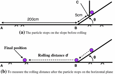
Determination of rolling damping based on the particle rolling test from an inclined plane
Fig. 4 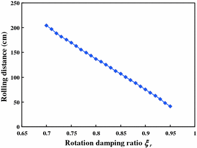
Influence of rotation damping ratio ξ r on the rolling distance


4 Verification of the Proposed Model
4.1 Repose Angle Test of Chalk Rod Assembly
To examine the validity of the proposed model, this study shows a comparison of these simulations, with the actual results of rod assemblies under a series of repose angle tests. Figure 5 shows the repose angle test for an equal-sized chalk rod assembly. The chalk rod assembly was first arranged in order and placed in a wood container measuring 70-mm width and 150-mm height. Three types of rod packing were conducted, containing 8, 12, and 16 layers of rods, and each layer had seven rods. The left wall of the container was then removed immediately, and the rods started sliding and rolling. The rod assembly finally formed a stable pile, and the angle of repose could be determined. During the experimental process, a digital camera recorded the whole sliding behavior and the reposed patterns.

Schematic illustration of the repose angle test
Figure 5b shows a DEM model for simulating the model tests. A specimen with the same packing of chalk rod assembly was constructed, and the same set of parameters (Table 1) was adopted for subsequent analysis. The lateral side and the bottom of the model served as rigid boundaries, and the top of the model was set as an unconstrained boundary. For the left side of the model, a moveable boundary was adopted to simulate the movement of the wall. As the wall moved immediately, the rod assembly started to slide and roll and a stable pile could be observed.
4.2 Comparison with Other Models
This study also conducted and compared the simulation of other existing models. In this manner, the characteristics of the proposed model could be highlighted. Existing models include (1) viscous damping, (2) local damping, and (3) a combination of viscous damping and local damping. For the viscous damping model, the normal and shear damping forces were added to the contact force during the particle motion. These damping forces can be expressed as
where F dn and F ds are the normal and shear damping forces, respectively. The damping forces inhibit motion.
The generalized damping forces for the local damping model (PFC2D (2004) are
where \( \left( {F_{i}^{\text{d}} } \right)_{\text{l}} \) is the generalized local damping force, F i is the generalized force, \( \dot{x}_{i} \) is the generalized velocity, and α is the local damping constant.
The last model considers both the viscous damping and local damping forces. Table 1 shows a summary of the required parameters for these models.
4.3 Results of the Repose Angle Tests
Figures 6, 7, and 8 show the reposed patterns of the model test and the proposed model for different packing of particles. These simulations are in agreement with the experimental results. Figures. 9, 10, and 11 show comparisons of other existing models, that is, those of the viscous damping model, the local damping model, and the combined damping model, respectively. Figure 9 shows that the particles based on the viscous damping model would not stop rolling. The reposed patterns were not obtained unless the simulation was terminated forcibly and were significantly different from the actual results. The simulations based on the local damping model (Fig. 10) exhibit higher reposed angles than experimental results. Because of excessive energy dissipation, the particles reached a stable state in a shorter period. The combined damping model displayed in Fig. 11 shows improved results compared to those of the other existing models, but still shows higher reposed angles than the experimental results.

Comparison between simulation and experimental results of the repose angle test with eight layers of rods

Comparison between simulation and experimental results of the repose angle test with 12 layers of rods

Comparison between simulation and experimental results of the repose angle test with 16 layers of rods

Simulations of the repose angle test using the linear contact model with viscous damping

Simulations of the repose angle test using the linear contact model with local damping

Simulations of the repose angle test using the linear contact model combined with local damping and viscous damping
To further compare the simulation and the experiments quantitatively, this study defines the simulated accuracy as
This study uses five indices of the reposed pattern, including (1) the average thickness of repose, (2) length of repose, (3) height of repose, (4) top length of repose, and (5) the repose angle (Fig. 12). According to Eq. 10, Fig. 13 shows the simulated accuracy of the proposed model, local damping model, and combined damping model. However, the results of the viscous damping model are not shown in Fig. 13, because it approaches 0% of accuracy. Figure 13a shows a test of eight layers of rods, revealing that the average accuracy of the proposed model is 90.9% and that Index 5 (repose angle) has the highest accuracy. Figure 13b, c shows that the average accuracies of the proposed model are 92.4 and 90.0%, respectively. The proposed model produces simulations that are superior to the other models, and has an average accuracy that ranges from 61.5 to 83.8%. Therefore, the proposed model simulates the characteristics of the reposed patterns accurately.

Indices to evaluate the predicted performance of models

Comparison of the simulated accuracy of contact models according to the indices
5 Application to the Landslide Model Test
In this study, we also simulated landslide behavior by using the proposed model. A corresponding landslide model test with a chalk rod assembly was also performed to compare the appropriateness of the numerical model and the set parameters. Figure 14a shows a slope of chalk rod assembly with an angle of 75°. The slope was 330-mm wide and 170-mm high, and a lateral wood wall (friction angle = 33°) was set on the left side to function as a retaining wall. After the wall was removed, a digital camera recorded the whole sliding behavior (Fig. 14a). The resulting failure pattern and landslide processes were compared with those from DEM analysis. The failure pattern shows that the maximum thickness of the repose was 68 mm, the length of the repose was 229 mm, and the repose angle was approximately 40°. Figure 14b shows the simulated results of the proposed model. The sliding processes of the simulation are in agreement with those of the model test, and the final repose patterns are also similar. However, discrepancies of the corresponding time exist between the simulation and the test (i.e., the simulation requires more time). The error is mainly because the damping parameters are obtained from the back-calculation of the restitution energy and the rolling distance, and not from the real-time motion. Therefore, this additional time is the limitation of the proposed model and further studies are required.

Experimental and simulated results of the landslide model test
Figure 15 shows a comparison of the images for the failure pattern of the test and the simulated results of the three types of contact models. The results of the viscous damping model (Fig. 15c) exhibit a gentler slope of the failure pattern than that of the model test, and a significant gap appears on the top of the slope that does not appear in the actual result. Conversely, a substantially steeper pattern appears in the local damping model, and most particles stay in the original positions (Fig. 15d). The comparison displayed in Fig. 15b shows that the proposed model achieved simulation results that were superior to those of the other models.

Comparison of three types of models on the landslide model test
6 Conclusion
This study proposed an innovative model of the rolling resistance of circular particles based on DEM simulation. The proposed model contains two major concepts: eccentric circle and local rotational damping. The mass center of a circular particle is first adjusted slightly for eccentricity to provide the rotational stiffness. A local rotational damping is then adopted to dissipate energy in the rotational direction. The model was tested for modeling repose tests and landslide behavior of chalk rod assemblies and shows a good capability to simulate actual behavior under different packing types. In this study, we also conducted and compared simulations using other existing models, showing that the proposed model achieved the best performance. In conclusion, particle rolling simulation using the proposed model appears to proximate the actual particle trajectory, making it useful for various applications.
Abbreviations
- C n :
-
Normal damping constant
- C s :
-
Shear damping constant
- e :
-
Eccentric value
- E :
-
Elastic modulus
- E r :
-
Restitution ratio of energy
- F n :
-
External normal force
- F s :
-
External tangent force
- F dn :
-
Normal damping force
- F ds :
-
Shear damping force
- (F d i )l :
-
Generalized local damping force
- F i :
-
Generalized force
- h 0 :
-
Falling height
- \( h_{0}^{'} \) :
-
Rebounding height
- K n :
-
Normal stiffness
- K s :
-
Shear stiffness
- M e :
-
Moment due to the eccentricity
- M r :
-
Moment during the rotation
- M dr :
-
Damping moment
- m :
-
Mass
- R :
-
Radius of a circle block
- U n :
-
Normal displacement
- \( \dot{U}_{\text{n}} \) :
-
Normal velocity
- \( \ddot{U}_{\text{n}} \) :
-
Normal acceleration
- U s :
-
Shear displacement
- \( \dot{U}_{\text{s}} \) :
-
Shear velocity
- \( \ddot{U}_{\text{s}} \) :
-
Shear acceleration
- \( \dot{x}_{i} \) :
-
Generalized velocity
- α:
-
Local damping constant
- \( \dot{\theta } \) :
-
Angular velocity
- \( \ddot{\theta } \) :
-
Angular acceleration
- ν :
-
Poisson’s ratio
- ξ n :
-
Normal damping ratio
- ξ s :
-
Shear damping ratio
- ξ r :
-
Rotational damping constant
- Φ:
-
Eccentric angle
- ψ:
-
Inter-rod friction angle
References
Calvetti F, Emeriault F (1999) Interparticle forces distribution in granular materials: link with the macroscopic behaviour. Mech of Cohes-Frict Mater 4:247–279
Chang YL, Chu BL, Lin SS (2003) Numerical simulation of gravel deposits using multi-circle granule model. J Chin Inst Eng 26(5):681–694
Chang YL, Chen CY, Xiao AY (2011) Non-circular rock-fall motion behavior modeling by the eccentric circle model. Rock Mech Rock Eng 44:469–482
Cho N, Martin CD, Sego DC (2007) A clumped particle model for rock. Int J Rock Mech Min Sci 44(7):997–1010
Cundall PA (1971) A computer model for simulating progressive, large scale movement in blocky rock systems. Proc Symp Int Soc Rock Mech, Inst Civ Eng Nancy, France 2(8):129–136
Cundall PA, Strack ODK (1979) A discrete numerical model for granular assemblies. Geotechnique 29(1):47–56
Elperin T, Golshtein E (1997) Comparison of different models for tangential forces using the particle dynamics method. Physica A 242:332–430
Hentz S, Daudeville L, Donze F (2004) Identification and validation of a discrete element model for concrete. J Eng Mech 130(6):709–719
Hsieh YM, Li HH, Huang TH, Jeng FS (2008) Interpretations on how the macroscopic mechanical behavior of sandstone affected by microscopic properties—revealed by bonded-particle model. Eng Geol 99:1–10
Oda M, Iwashita K (1999) Mechanics of granular materials. A.A. Balkema, Rotterdam
Oda M, Kazama H (1998) Micro-structure of shear band and its relation to the mechanism of dilatancy and failure of granular soils. Geotechnique 48(1):1–17
PFC2D (2004) Particle Flow Code in 2 Dimension Version 4.0. Itasca Cons Group, Minneapolis
Potyondy DO, Cundall PA (2004) A bonded-particle model for rock. Int J Rock Mech Min Sci 41:1329–1364
Press WH, Teukolsky SA, Vetterling WT, Flannery BP (1992) Numerical recipes in C. Cambridge University Press, Cambridge
Schopfer MPJ, Abe S, Childs C, Walsh JJ (2009) The impact of porosity and crack density on the elasticity, strength and friction of cohesive granular materials: insights from DEM modeling. Int J Rock Mech Min Sci 46:250–261
Sitharam TG, Vinod JS, Ravishankar BV (2008) Evaluation of undrained response from drained triaxial shear tests: DEM simulations and experiments. Geotechnique 58(7):605–608
Utili S, Nova R (2008) DEM analysis of bonded granular geomaterials. Int J Numer Anal Meth Geomech 32:1997–2031
Wang YH, Leung SC (2008) A particulate-scale investigation of cemented sand behaviour. Can Geotech J 45:29–44
Zhou YC, Wright BD, Yang RY, Xu BH, Yu AB (1999) Rolling friction in the dynamic simulation of sandpile formation. Physica A 269:536–553
Zhou YC, Xu BH, Yu AB, Zulli P (2002) An experimental and numerical study of the angle of repose of coarse spheres. Powder Technol 125:45–54
Acknowledgments
The authors are grateful to the chief editor and anonymous reviewers who kindly provided professional suggestions for this work.
Open Access
This article is distributed under the terms of the Creative Commons Attribution License which permits any use, distribution, and reproduction in any medium, provided the original author(s) and the source are credited.
Author information
Authors and Affiliations
Corresponding author
Rights and permissions
Open Access This article is distributed under the terms of the Creative Commons Attribution 2.0 International License (https://creativecommons.org/licenses/by/2.0), which permits unrestricted use, distribution, and reproduction in any medium, provided the original work is properly cited.
About this article
Cite this article
Chang, YL., Chen, TH. & Weng, MC. Modeling Particle Rolling Behavior by the Modified Eccentric Circle Model of DEM. Rock Mech Rock Eng 45, 851–862 (2012). https://doi.org/10.1007/s00603-012-0227-0
Received:
Accepted:
Published:
Issue Date:
DOI: https://doi.org/10.1007/s00603-012-0227-0