
Abstract
Sequence stratigraphy has been applied in a wide range of scales of time and space, from decimeter-thick layers formed within hours to kilometer-thick basin fills formed during hundreds of millions of years. The traditional approach to practice sequence stratigraphy in this wide range of scales is to subdivide the sediment piles into an ordered hierarchy of sequence cycles of different duration and different architecture. An alternative are scale-invariant models with fractal characteristics. Published data confirm two predictions of the ordered-hierarchy model: sequences of very short duration (<1 × 10³ years) are parasequences bounded by flooding surfaces, very long sequences (>200 × 106 years) are symmetrical transgressive–regressive cycles. However, the sequence record in the range of 1 × 10⁴–200 × 106 years, the principal domain of sequence stratigraphy, shows a rather irregular succession of sequences with variable symmetry and bounded by flooding surfaces or exposure surfaces. For these time scales, scale-invariant models are a good first approximation, particularly because the evidence for scale-invariance and randomness in the stratigraphic record is strong: Frequency spectra of sea-level change as well as rates of sedimentation and rates of accommodation change plotted against length of observation span show basic trends indistinguishable from random walk. These trends, combined with scale-invariant sequence models may be the most efficient tools for across-the-board predictions on sequences and for locating islands of order in the sequence record.
Introduction
The concepts of stratigraphic sequences (Sloss 1963) and sequence stratigraphy (Vail et al. 1977) are among the most significant developments in sedimentary geology in the past half-century. Sloss’ (1963) concept of stratigraphic sequences arose from the well-known history of transgressions and regressions on cratons, i.e. processes in a time frame of 107–108 years. The starting point for the sequence stratigraphy of Vail et al. (1977) were seismic data of large basins and continental margins, i.e. data in the stratigraphic time frame of 106–108 years. The intensive use of data from boreholes and outcrops expanded the sequence-stratigraphic technique to stratigraphic scales far below the million-year range. At present, sequence stratigraphy is applied at time scales of 10−1–108 years, i.e. over nine orders of magnitude of years, and to stratigraphic bodies of 10−2–103 m, i.e. five orders of magnitude in thickness. The possibilities and problems that arise from practicing sequence stratigraphy in this wide range of temporal and spatial scales are the subject of this review. I first present two contrasting models of sequence stratigraphy—ordered hierarchy versus scale invariance of stratigraphic sequences—and subsequently assess to what extent these models fit the observational data.
It should be noted that the wide range of spatial scales is easier to handle than the large variation of temporal scales. Sadler and Strauss (1990) succinctly state the problem of long time spans in sedimentary geology: “…Some modern sites of deposition have been monitored continually, but only for time spans that fall far short of the time it would take to accumulate a typical stratigraphical section…” In other words, the present may be the key to depositional structures and facies of the past but it is a rather imperfect guide to how the stratigraphic record actually forms. A specific problem concerns process rates. The rates of deposition and of accommodation change, the two fundamental controls of stratigraphic sequences, have been shown to change with the length of the time span of observation. Modern rates are meaningless unless they are scaled to the time span under consideration. Therefore, plots of process rates versus time will figure prominently in this report.
Contrasting models of sequence stratigraphy
Ordered hierarchy of stratigraphic sequences
The pioneer papers on sequence stratigraphy postulated that stratigraphic sequences formed an ordered hierarchy of cycles, controlled by an analogous hierarchy of eustatic sea-level cycles (Vail et al. 1977, p 83–97). Three orders of sea-level cycles were recognized: first-order cycles of 200–300 Myr duration, second-order cycles of 10–80 Myr, and third-order cycles of 1–10 Myr duration. Second and third order cycles were found to have very similar architecture, described by the “slug-model” of sequences (Fig. 1; Vail 1987; Posamentier and Vail 1988). First-order cycles were viewed as symmetrical alternations of transgressive and regressive stratigraphic successions. This difference in architecture was attributed to differences in eustatic sea-level cycles. Sea-level movements associated with first-order sequences were depicted as nearly symmetrical waves in the time domain, sea-level cycles associated with second and third- order sequences were assumed to be strongly asymmetrical with slow rises and rapid falls (Vail et al. 1977).

a Standard (“slug”) model of stratigraphic sequences (Vail 1987, modified). b Interpretation of the model components in terms of rates of accommodation change and rates of sediment supply (Schlager 1992, modified). Most of the features in the model depend on the balance of the two rates. However, the exposure surface on top of the marine highstand tract of the preceding sequence and the (orange) lowstand systems tract can only form if the rate of accommodation creation is negative, i.e. if sea-level has fallen, regardless of the rate of sediment supply
The system of orders was significantly expanded by Van Wagoner et al. (1988) who reported that the building blocks of third-order sequence cycles were sequence cycles bounded by flooding surfaces rather than exposure surfaces; the term “parasequence” was introduced for these shorter sequence cycles below the classical third-order sequences.
In an important overview of the ordered hierarchy of sequences, Vail et al. (1991) identified tectonics, eustasy, and sedimentation as the basic controls on sequences with eustasy as the principal cause of the hierarchy. First-order cycles were attributed to tectono-eustasy, i.e. changes in the rates of sea-floor spreading and the formation/destruction of supercontinents. Cratons were found to present the best records of these symmetrical transgressive–regressive cycles. Cycles of second through fifth order were called sequence cycles. Second and third order cycles were assumed to have typical sequence architecture with lowstand, transgressive and highstand systems tracts and exposure surfaces as sequence boundaries. Cycles of fourth and fifth order were assumed to show either classical sequence architecture (“simple sequences”) or parasequence architecture, i.e. shoaling successions bounded by flooding surfaces and devoid of lowstand tracts.
Duval et al. (1998) studied long cycles and their potential for predicting major hydrocarbon source rocks. The study includes an overview of the architecture of the different orders of sequence cycles (Fig. 2). In contrast to Vail et al. (1991), second-order cycles are viewed as symmetrical and different from the asymmetrical cycles of the third order.

Sequence architecture in the ordered-hierarchy model of sequences. Long sequence cycles (first and second order) are rather symmetrical transgressive–regressive units. Third-order cycles are classical sequence cycles bounded by exposure surfaces and consisting of lowstand, transgressive and highstand systems tracts. Cycles of fourth order and shorter are parasequences, i.e. shoaling upward successions bounded by flooding surfaces. After Duval et al. (1998), modified
Both Vail et al. (1991) and Duval et al. (1998) define sequence orders by duration but there is also a systematic change in depositional architecture with decreasing duration. First-order cycles (according to Duval et al. 1998 also second-order cycles) are symmetrical transgressive–regressive successions composed of asymmetrical third-order cycles bounded by exposure surfaces. Third-order cycles, in turn, are composed of asymmetrical parasequences (fourth order and lower) bounded by flooding surfaces.
Scale-invariant stratigraphic sequences
Randomness and scale-invariance in the sediment record
Scale-invariance is a basic property of many geologic features, such as faults, folds and the stratigraphic succession of layers. The need to put scales on photographs of such features indicates their scale-invariance. The following examples of scale-invariance are particularly relevant for sedimentary geology in general and sequence stratigraphy in particular.
-
Many populations of sedimentary units (thickness of beds or formations, duration of stratigraphic sequences) exhibit lognormal frequency distributions. This implies that in most of the population frequency decreases exponentially with linearly increasing class size. Significant modes in abundance are lacking. These findings strongly suggest that the basic structure of the sediment record is that of a continuum with the hierarchy of orders representing rather arbitrary subdivisions of this continuum (Drummond and Wilkinson 1996).
-
Characteristic elements in the architecture of sediment accumulations have been shown to be invariant over wide ranges of spatial and temporal scales. Thorne (1995) developed a quantitative model of the triad of topset–foreset–bottomset, a critical element in sequence architecture. He argued that this architecture remains virtually invariant for vertical scales of 100–103 m. Van Wagoner et al. (2003) showed that the plan-view patterns of sediment accumulations fed by a point source, such as deltas and turbidite fans, remain invariant on scales of about 14 orders of magnitude in area. Posamentier et al. (1992) showed that a meter-scale delta that formed in a drainage ditch within hours exhibits many characteristic features of stratigraphic sequences. Scale-invariance also has been observed for basic patterns of biological precipitates, such as the formation of rimmed carbonate platforms (Fouke et al. 2000; D’Argenio 2001).
-
The power spectrum of sea-level change has been compiled for 15 orders of magnitude of frequency (Harrison 2002). The dominant trend is that power varies with the square of the reciprocal frequency—a characteristic of random walk. Deviations from this trend, indicating more ordered patterns, form “islands of order” in the overall trend.
-
Rates of accommodation change have been compiled by Sadler (1994) for time scales of days to hundreds of millions of years. Figure 3 shows the part most relevant for sequence stratigraphy, i.e. the time scales of 103–108 years. Sadler’s data were generated in two independent ways: (1) rates calculated from depth below modern sea level of peritidal carbonates, i.e. sediments that were deposited within few meters of mean sea level; and (2) the sums of independent estimates of mean subsidence rates and rates of eustatic sea-level change. The agreement between the two datasets is impressive. The basic trend for both sets is that the change in accommodation rates is proportional to the reciprocal square root of time, again a trend characteristic of random walk.
Fig. 3 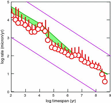
Rates of accommodation creation as a function of the time span of observation. Red circles with bar represent mean and one standard deviation of accommodation rates, estimated from modern depths below sea floor of ancient peritidal carbonates. Green band: sum of mean subsidence rate and the upper envelope of rates of sea-level change estimated from sea-level histories (all data from Sadler 1994, modified). Note overall good agreement between red and green data set. Data from subsidence and sea-level histories show smooth trend, peritidal deposits show more fluctuations, most notably in the range of 104–105 years. However, the basic trend of both data sets is close to that of a random walk (magenta lines)
-
Sediment accumulation rates decrease with increasing time span of observation (Fig. 4; Sadler 1981, 1999; Plotnick 1986). In the time domain of days to hundreds of millions of years, the basic trend of sedimentation rates is to decrease with the reciprocal square root of time. As with the accommodation record, this trend is typical of random walk. Sadler (1999, p. 39) noted that the residuals of this first-order trend are not random: sedimentation rates of very short time spans show steeper trends (high proportion of time represented by hiatuses), very long-term rates show flatter trends (lower proportion of time in hiatuses). Sadler (1999) tentatively attributes this pattern to the increasing role of lithospheric subsidence with increasing time span.
Fig. 4 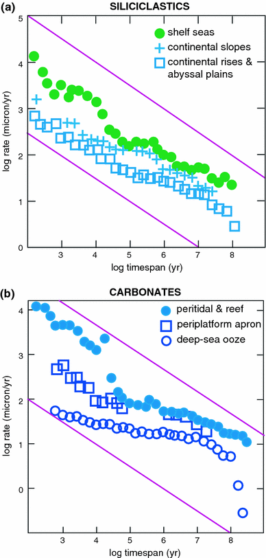
Sedimentation rates of siliciclastics and carbonates as a function of the time span of observation (after Sadler 1999, modified). In both sediment families rates decrease with increasing time span and the basic trend is very close to the trend of random walk (magenta lines). Trends in deep-sea environments are rather smooth; trends in shallow-water environments have steps and plateaus, indicating bundling of hiatuses in certain intervals probably caused by periodic sea-level cycles. Distinct step between 104 and 105 years in both groups approximately coincides with pronounced orbital cycles


Fractal model of scale-invariant sequence stratigraphy
The strong evidence for scale-invariant patterns in the stratigraphic record and the persistent problems with defining orders in the sequence hierarchy led to the formulation of a scale-invariant model for tropical carbonate sequences (Schlager 2004). The model postulates the following:
-
The sequence record has fractal characteristics, i.e. longer sequences are upscaled versions of shorter sequences.
-
There are two basic building blocks of the sequence record: S sequences (or “standard sequences”) are bounded by exposure surfaces and are commonly endowed with a lowstand systems tract; P sequences (or parasequences) are bounded by flooding surfaces and devoid of lowstand tracts. All sequences include transgressive and highstand tracts.
-
In the spatial and temporal validity range of the model, P and S sequences form random alternations. Moreover, the shelf-margin trajectories of long-term prograding systems have fractal characteristics.
Figure 5 summarizes the characteristics of the scale-invariant sequence model for tropical carbonate deposits. The model was proposed for the time range of 103–106 years. The lower limit of this time interval is determined by the rates of soil processes since the discrimination between P sequences and S sequences depends first on the development of soil features for recognizing “exposure” in sedimentological terms. Build-up of organic matter, one of the fastest soil processes, takes 103 years or more to reach significant levels (Birkeland 1999). Accretion of calcretes in carbonate domains may proceed at rates of several millimeters/103 years (Robbin and Stipp 1979). Therefore, a lower limit of 103 years for the model seems reasonable. The upper limit is determined by lack of data for determining the P:S ratio beyond the domain of 106 years. The time limits, in turn, largely determine the limits in space. In the time range of 103–106 years, the thickness of sediment bodies typically falls in the range of 100–103 m, their correlative lateral extent is approximately 101–105 m.

Scale-invariant (fractal) sequence model (after Schlager 2004, modified). The model assumes that in the time range of 103–106 years, sequence cycles of standard type, i.e. with lowstand tracts and bounded by exposure surfaces, and cycles of parasequence type devoid of lowstand tracts and bounded by flooding surfaces, follow each other in random succession. The lower limit of the validity range of the model is determined by the rate of soil processes, the upper limit by lack of sufficient data, notably lack of intact passive margins
The proportions of P and S sequences in well-documented carbonate successions were found to be about 1:1 (Fig. 6). However, equal proportions of P and S sequences are not an intrinsic property of the model. It is probable that with increasing duration of cycles, S sequences (exposure boundaries) become more abundant. Moreover, the percentage of P sequences (bounded by flooding surfaces) may be higher in siliciclastics because during transgressions, soils on siliciclastics are more easily removed than on the fast-lithifying carbonates. The postulate that a significant number of flooding surfaces serve as sequence boundaries in the domain of >1 × 10⁶ years is based on the carbonate record (e.g. Erlich et al. 1990; Saller et al. 1993; Sattler et al. 2009; Zampetti et al. 2004). Carbonate systems may be terminated by exposure or they may drown. Drowning implies that the growth potential of the system falls below the rate necessary to keep up with the rate of relative sea-level rise. Drowning unconformities are essentially flooding surfaces. They are seismically prominent features that repeatedly have been designated as sequence boundaries, for instance in the papers listed above. Schlager (1999) proposed to distinguish them as type-3 sequence boundaries from the exposure-related type-1 and type-2 boundaries. Another feature of the model, the fractal nature of shelf-edge trajectories, is illustrated in Fig. 7.

Abundance of standard sequences (bounded by exposure surfaces) and parasequences (bounded by flooding surfaces) in well-documented successions of peritidal carbonates. Upper panel sequences of 1 × 10⁶ years and longer, lower panel sequences shorter than 1 × 10⁶ years. In both categories, the ratio of standard sequences and parasequences is about 1:1. After Schlager (2004), modified

Test for fractal nature of shelf-edge trajectories. a Example of shelf-margin trajectory of Cenozoic carbonate platform in the Bahamas (Eberli and Ginsburg 1988). b Results of box-counting technique (Turcotte 1997) applied to Bahamian example as well as prograding shelf margin off Alabama and off New Jersey (Greenlee 1988). Plots show box size versus number of boxes required to cover the trajectory. Fractal nature of trajectories is indicated by the power-law relationship (linear trend in bi-logarithmic plot) of box size versus number of boxes. All trajectories mapped and analyzed by the author
T–R stratigraphy as a basis of scale-invariant sequence models
T–R sequence stratigraphy subdivides stratigraphic successions into transgressive–regressive couplets with the sequence boundary at the top of the regressive systems tract (Embry and Johannessen 1992; Embry 1993; Catuneanu 2006). The concept builds on the fact that most shallow-water deposits can be subdivided into shoaling and deepening intervals, frequently corresponding to intervals of increasing and decreasing influence from land in deep-water deposits. This principle holds for a wide range of scales in time and space and could serve as the basis of a scale-invariant model of stratigraphic sequences.
A hierarchy of cycles has been proposed for T–R sequences (Embry 1993; Catuneanu 2006, p. 331). Sequence ranks are distinguished by the range of base-level fall and the degree of change in sedimentary regime at the R/T sequence boundaries as well as by the degree of deformation that occurred during the formation of the boundary hiatus. However, the internal architecture of T–R sequences does not change in this hierarchy. Consequently, the concept could provide a valid basis for scale-invariant sequence models.
The elegant simplicity and broad applicability of T–R stratigraphy come at a price. The concept does neither differentiate between normal and forced regression, nor recognize the lowstand systems tract as a separate entity (compare Fig. 1). Consequently, T–R stratigraphy does not distinguish between (sea-level related) changes in accommodation and changes in sediment supply.
Discussion
Critique of the ordered-hierarchy concept
Testimony of random walk
A common argument for the existence of an ordered hierarchy of sequence cycles is that one can see the superposition of cycles in the data—in outcrop, in wireline logs, in curves of relative sea-level change and other stratigraphic records. These observations usually are correct but in this qualitative fashion, they contribute little to the discrimination between ordered hierarchy and randomness. The important point, often neglected, is that superposition of shorter and longer trends are also a characteristic of random processes such as Brownian walk. Thus patterns as shown in Fig. 8 are no argument for an ordered hierarchy of cycles unless time series analysis or other quantitative techniques indicate that a particular pattern arises from the superposition of cycles of different periods. Settling the question of order versus randomness is particularly important for short cycles in the sediment record. Very long cycles, such as the two-first-order cycles of the Phanerozoic (e.g. Harrison 2002, Fig. 2) are so long and their effects are so large that the geologic record shows them clearly as individual cycles, probably linked to the formation and destruction of supercontinents. For sedimentary geologists, it is not particularly urgent to know if these long cycles are driven by chaotic or ordered, periodic processes. The more urgent question for sedimentologists and stratigraphers are the sequences of lower rank (second-order and shorter), in particular the cycles in the range of 103–105 years that frequently determine the heterogeneity of reservoirs of water or hydrocarbons in the subsurface.

Brownian noise and walk. a Brownian noise, i.e. a succession of random numbers varying between –1 and +1, with mean of 0. b Brownian walk, i.e. the plot of the running sum of the numbers in (a). Superposition of shorter and longer trends is a typical attribute of Brownian walk but does not imply ordered hierarchy of cycles. After Harrison (2002)
Defining ranks by duration
The durations proposed for the various ranks (or orders) of sequence cycles vary considerably. Schlager (2004) and Catuneanu (2006, p. 330) compared published definitions. Figure 9 presents a comparison of important papers. It is clear that the differences are large. In fact, the extreme positions for each order boundary differ at least by ½ order of magnitude, in some instances the differences exceed a full order of magnitude. Moreover, opinions do not seem to converge in the course of time, yet convergence would be expected if the classification reflected some ordered pattern in nature. The fact that boundaries frequently are chosen at full powers of ten also indicates that the orders are subdivisions of convenience in a continuum, comparable to the subdivisions of the metric length scale. The somewhat arbitrary nature of the separation of second and third order cycles is also illustrated by the broad overlap of their respective durations in the sea-level curve of Haq et al. (1987), shown in Fig. 10. The duration of second-order cycles in the epochs with good chronostratigraphy frequently equals the duration of third-order cycles in the epochs with poorer chronostratigraphy.

Durations of orders of stratigraphic sequences as proposed by various authors. In most instances, order boundaries of different authors differ by more than half an order of magnitude; for fourth, fifth and sixth orders the differences are even larger. Moreover, opinions do not seem to converge with time (oldest publications at the top of each column). After Schlager (2004), modified; based on classifications in Vail et al. (1977), Williams (1988), Van Wagoner et al. (1990), Carter et al. (1991), Vail et al. (1991), Reid and Dorobek (1993), Duval et al. (1998), Lehrmann and Goldhammer (1999)

Duration of sea-level cycles of second and third order in the estimated eustatic curve of the Mesozoic and Cenozoic of Haq et al. (1987). The modes of the two categories are distinctly different but the ranges broadly overlap because the third-order cycles of the chronologically less constrained epochs have durations similar to the second-order cycles of the well-dated epochs. After Schlager (2004), modified
Rank-specific sequence architecture
The link between sequence duration and sequence architecture is not as straightforward as indicated by Vail et al. (1991) and Duval et al. (1998). There can be little doubt that duration has some influence on sequence architecture. A comparison of very short and very long sequence cycles shows this: the longest cycles, with durations of 108 years tend to be rather symmetrical transgression-regression cycles; they usually are observed on cratons and exposure surfaces are the logical sequence boundaries (Sloss 1963; Vail et al. 1977; Duval et al. 1998). In contrast, the shortest cycles considered by sequence stratigraphers, units of 101–102 years, tend to be strongly asymmetric, shoaling-upward successions bounded by flooding surfaces. The bounding surface at the top is a flooding surface because the time is too short to form geologically recognizable soil horizons (see discussion on scale-invariant models below). However, data on sequences of 103–107 years duration, the interval most relevant to practical application of sequence stratigraphy, do not conform well to the ordered-hierarchy model.
Particularly unsatisfactory is the notion that the building blocks of classical sequences (approximate domain 105–106 years) are parasequences bounded by flooding surfaces (Van Wagoner et al. 1990; Duval et al. 1998). Vail et al. (1991) already indicated that the building blocks of third-order cycles may be either parasequences bounded by flooding surfaces or “simple sequences” bounded by exposure surfaces. The growing attention on the falling-stage and late highstand systems tracts produced many more examples of exposure-bounded subunits (e.g. Plint and Nummedal 2000, p. 8; Posamentier and Morris 2000). In carbonates, Schlager (2004) found about equal proportions of exposure boundaries and flooding boundaries in sequences shorter and longer than 1 × 10⁶ years. Schlager’s (2004) data were compiled from numerous field sections, each measured at one location. Studies examining the lateral variability of boundaries in carbonates (e.g. Sattler et al. 2005) indicate that the surface characteristics may also change laterally from exposure to flooding and vice versa. In summary, it seems that in a wide range of time scales, the sequence record consists of a mix of units bounded by flooding surfaces and units bounded by exposure surfaces and these characteristics may change laterally.
Case-by-case approach to sequence ranking
After extensive literature review, Catuneanu (2006, p. 332) concludes that “no universally applicable hierarchy system…has been devised yet” and proposes to assign sequence ranks on a case-by-case basis. This approach starts with assigning top rank (=first order) to the entire sediment fill of a particular basin and defining lower-rank sequences as appropriate. This approach undoubtedly has merit. It should be noted, however, that in many respects it represents the opposite of what the founders of sequence stratigraphy had in mind. Catuneanu (2006) argues for local or regional subdivisions instead of application of globally established orders to regional datasets. An attractive aspect of the case-by-case approach is that the search for global signals may still be carried out once a regional scheme is in place.
The examples of first-order sequences identified with this method vary in duration from 5 × 10⁶ years to >600 × 106 years (Catuneanu 2006, p. 334). On the short side, this range may easily be extended by another order of magnitude. There are, for instance, pull-apart basins whose entire history covers <5 × 10⁵ years (e.g. Van der Straaten 1992). The practical implication of the approach of Catuneanu (2006) is that first-order sequences may vary in duration in the range of <5 × 10⁵–600 × 106 years. Consequently, first-order sequences in the case-by-case approach may correspond to sequences of first to fourth order in the ordered-hierarchy models. The case-by-case approach therefore implies that the link between cycle architecture and cycle duration of the ordered-hierarchy model has to be abandoned.
Critique of the concept of scale-invariant sequences
Randomness is not a particularly appealing property, certainly not in the context of historic documentation. Most historians would find it utterly unsatisfactory if they had to describe human history as a random succession of war and peace, economic growth and recession, etc. Earth scientists, too, may be dissatisfied by the prospect of having to describe an important document of earth history, the sequence record, as a random succession of rises and falls of sea level and waxing and waning sediment supply. However, there is no reason for dissatisfaction. A major task of earth scientists is to make predictions about unknown parts of the subsurface. In this capacity, any concept that helps improve subsurface prediction is welcome. The scale-invariant model may accomplish two tasks with regard to geologic prediction. First, it provides a baseline from which one can estimate the degree of order in different parts of the sequence record and identify the ordering principle (e.g. orbital or annual rhythms). Second, for those parts of the record that closely follow the trend of random walk, the statistics of the random case may be used as predictor. The statistical properties of random events are predictable provided the number of samples is sufficiently large. Casinos and insurance companies do well with this principle.
The term “scale-invariant” also merits some discussion. Scale-invariance does not mean that scale is irrelevant for the concept. On the contrary, the applicability of scale-invariant models ends where processes that are crucial for the development of diagnostic features of sequences have a characteristic duration or a characteristic size. Important limits in time or space for the scale-invariant sequence model have already been mentioned and are further evaluated below.
Time limit set by soil formation
The development of exposure surfaces requires a certain length of time, namely the interval required to develop soil features. This seems the only way to distinguish between the marine sediment surfaces exposed to the air for hours or days, e.g. during a tidal cycle, and surfaces exposed long enough that terrestrial conditions could be established. Schlager (2004) estimates that about 1,000 years would be required to form stratigraphically preservable, diagnostic soil features in carbonate rocks. Carbonate rocks probably preserve evidence of exposure in short cycles readily because of extensive early cementation. In siliciclastics, most soils are washed away before they can lithify. The best evidence for exposure of siliclastic shelves commonly occurs in incised river valleys that require more time to develop than thin soils on alluvial plains. This may be one reason for the postulate that units shorter than third-order sequences are bounded by flooding surfaces.
Time limit set by plate tectonics
Schlager (2004) assumed an upper time limit of 106 years for the scale-invariant sequence model because of scarcity of carbonate sequences in the domain of 107 years and beyond. Plate tectonics is thought to set this natural time limit in the following way. The ideal setting for studying the long-term sequence record is passive ocean margins with their prograding, retrograding, upstepping and downstepping shelf edges. However, the record of extant passive margins only extends 180–200 Myr back into the past and ocean crust is seldom more than 200 Myr old (e.g. Condie 1997). Consequently, the record of the first-order cycles (Duval et al. 1998) is based on the thin, epeiric sediment cover of cratons and fragments of ocean margins incorporated in mountain belts. It is unclear to what extent this change in the type of sediment record used for sequence studies influenced the architecture of the different orders postulated by Duval et al. (1998). It is clear, however, that testing the validity of the scale-invariant model for first-order cycles becomes nearly impossible under these circumstances.
Space limit set by the “mudline” in marine environments
The explorers of nineteenth century already knew that the content of clay and fine silt in marine sediments increases with depth and that there is a boundary, the “mudline”, below which cohesive fines dominate. Stanley et al. (1983) defined the mudline as the level below which the mud content no longer increases significantly with depth; they found this level between 20 and 1,000 m depth in modern oceans. George and Hill (2008) defined the mudline as the level where mean grain size falls below 0.063 mm and found it to lie between 6 and 194 m in modern oceans. Regardless of its formal definition and exact position, the mudline limits the scale-invariance of clinoforms. It implies that clinoforms extending below the mudline would have clay-dominated lower parts and would therefore be unable to maintain steep slope angles commensurate with the angles of repose of non-cohesive sediment. On the other hand, clinoforms associated with beaches and shallow shelves (Thorne 1995, p. 98) would nearly always be dominated by sand and rubble and therefore be able to maintain steep foresets over their full height.
Shelf-edge trajectories
The fractal nature of shelf-edge trajectories provides important geometric support for the fractal sequence model. It should be noted, however, that the tests of fractality are based on a very limited number of cases and that the fractal characteristics only extend over 1.5–1.8 orders of magnitude (Schlager, 2004). Consequently, the support for this part of the model is not particularly high but it is better than the mode of physics papers on fractals examined by Avnir et al. (1998).
Order in randomness
As mentioned above, the scale-invariant sequence model offers a baseline for estimating the degree of order in specific datasets. The studies of Harrison (2002) on sea-level fluctuations and of Sadler et al. (1993), Sadler (1994, 1999) on sedimentation rates and accumulation histories provide examples of subsets of ordered data in the overall random trend.
Harrison (2002) shows two trend lines in the power spectrum of the sea-level curve of Haq et al. (1987)—both are close to the trend of random walk. However, Harrison (2002) also shows that the eustatic sea-level curve derived from the oxygen-isotope ratios of marine plankton (SPECMAP curve, Imbrie et al. 1984) drastically differs from the random trend. The dataset has a much flatter trend and clearly shows the dominant orbital frequencies as individual peaks. The SPECMAP sea-level curve is an “island of order” in the random trend. It is important to note that the SPECMAP data were gleaned from the deep-sea record, using a chemical proxy of sea-level variation. Sequence-stratigraphic records of this time interval can be fit in this chronostratigraphic framework by correlating systems tracts and boundaries with the SPECMAP standard (Anderson et al. 2004). However, it has not been demonstrated that the procedure can be reversed and that the SPECMAP sea-level curve can be generated from the sequence record.
Sadler et al. (1993) and Sadler (1994) compiled and analyzed tens of thousands of sedimentation rates of peritidal carbonates. These rocks are particularly interesting for sea-level studies because their vast majority was deposited very close to sea level, in the top 10 m of the water column. Sedimentation rates show a pronounced deviation from the random trend, indicating the presence of frequent hiatuses in the time interval of 1.104–1.105 years (Fig. 4). This interval corresponds to major periods in the Earth’s orbital oscillations and Sadler (1994) indeed suggests that sea-level oscillations linked to orbital rhythms have caused this break in the random trend.
Peritidal carbonate deposits also illustrate the spread of opinions on the question of order versus randomness in stratigraphy. Sadler et al. (1993) and Sadler (1994) argued for at least intervals of order in the peritidal record. Drummond and Wilkinson (1996) emphasized the dominantly random nature of the peritidal successions based on the thickness-frequency distribution of beds in numerous case studies. Lehrmann and Goldhammer (1999) found patterns that ranged from random to ordered, based on facies-stacking patterns. Applying a quantitative measure of orderedness, Burgess (2008) confirmed the highly variable behavior of the Lehrmann–Goldhammer data.
Origin of randomness in sequence record
The definition of “random” in the natural sciences is less straightforward than it may seem and the earth sciences are no exception to this rule (e.g. Middleton 1991, p.208). In the present situation, it is more productive to invert the question and ask: what causes the islands of order in a trend that is indistinguishable from random walk? It seems that the islands of order invariably indicate data sets where one deterministic driver dominates the record. Examples are orbital variations and diurnal cycles (see Harrison 2002, Fig. 1 for examples). This observation strongly suggests that the random trend dominates where a dominant driver is absent such that the cumulative effect of several drivers of irregularly varying strength controls the record.
At the most basic level, the sequence architecture as described by Vail (1987), Van Wagoner et al. (1988) and Posamentier and Vail (1988) reflects the balance of the rate of accommodation change and the rate of sediment supply. However, each of these fundamental controls represents the sum of several different effects such as eustasy, crustal movements, etc. in the case of accommodation and topographic gradient, runoff, soil erodibility, strength, and location of ocean currents, etc. in the case of clastic sediment supply. Carbonate production mainly depends on climate, ocean chemistry and the state of organic evolution. The situation is further complicated by interactions among the drivers. Examples are the strong interactions between tectonic deformation and erosion, plate tectonics and ocean currents, sedimentation and subsidence, etc. Thus, it seems quite plausible that the superposition of many, partly interdependent drivers of highly variable strength lies at the root of the random features of the sediment record in general and the sequence record in particular. We can take measure from the stock market in this regard. Share prices result from the cumulative, orderly actions of many rational individuals. However, barring highly unusual events, the resulting curve is virtually indistinguishable from random walk.
Role of sequence stratigraphy in geology
From the outset, sequence stratigraphy had a dual function: it was a bridge between classical stratigraphy and seismic stratigraphy, and a tool in global correlation. The bridge function to seismics is not significantly affected by the debate about ordered hierarchy and scale-invariance in the sequence record. Sequence stratigraphy remains a powerful tool for interpreting seismic data and the importance of reflection seismics for petroleum geology and many fundamental questions in the earth sciences is undiminished.
The role as global chronologic standard suffers if the orders of sequence cycles are simply subdivisions of convenience in a stratigraphic continuum rather than part of an ordered temporal hierarchy of cycles. However, even where the sequence record represents a random succession of cycles, correlation—even at a global scale—is possible wherever individual events can be dated accurately or recognized by specific properties, such as the unconformity at the Cretaceous–Tertiary boundary. The absence of an ordered hierarchy of sequence cycles may be less damaging to the role of the sequence stratigraphy as a chronologic standard than the prominent function of unconformities in defining sequences. Unconformities represent major gaps in the record and thus greatly increase the uncertainties in dating and globally correlating sequences [see Miall (1992) for correlation experiments with random numbers; Kidwell (1988) for lateral diachroneity of traceable sequence boundaries and Sadler (1999, p. 32) for the effect of unconformities on sedimentation rates].
Standardizing sequence stratigraphy
The history of sequence stratigraphy as a concept is somewhat unusual. After initial work in the academic domain, a single group in industry developed the concept to a very advanced stage within about a decade. As a result, sequence stratigraphy re-entered the academic domain in highly mature and standardized form (Vail et al. 1977). Subsequent discussion in the open, academic domain was hampered by limited access to the seismic and drilling data on which the definition of sequence orders and the Phanerozoic sea-level curve were based. At least some of the problems with the ordered hierarchy of sequences may be the result of this unusual history of the concept. Regardless of the reasons, it seems that sequence stratigraphy is far less settled in its approach than other branches of stratigraphy. The current search for common ground (Catuneanu et al. 2009) is very useful but it also reveals how many of the basic principles still are subject to rather controversial debate (Helland-Hansen 2009). Standardization should proceed very cautiously on controversial issues. Evolving concepts must not be forced into a straitjacket by premature standardization.
Conclusions
-
Evidence for randomness and scale-invariance in the stratigraphic record is strong. Sedimentation rates, rates of accommodation change and the power of sea-level changes plotted against the duration of the observation span all show basic trends close to random walk. Periodic fluctuations, such as the Earth’s orbital oscillations, appear as islands of order in these basic trends.
-
A scale-invariant, fractal model of sequences honors the evidence for randomness in the stratigraphic record. For time scales of 104–106 years (and probably longer), the predictions of this model may serve as a baseline in the search for islands of order in the sequence record.
-
Definitions of orders of stratigraphic sequences vary widely and show no convergence in the course of time. In the time domain of 1 × 10⁴–200 × 106 years, the sequence orders defined by cycle duration seem to be subdivisions of convenience rather than a reflection of natural order. The proposition to define sequence orders relative to the life cycle of a sedimentary also implies that duration is a poor basis for defining sequence orders.
-
The visual impression of superposition of cycles in stratigraphic data is a poor argument for an ordered hierarchy of cycles. Random processes such as Brownian walk also share this property.
-
Sequence stratigraphy still is in a state of flux, even with regard to basic principles. Attempts to standardize the method should respect this and leave ample room for concepts to evolve.
References
Anderson J, Rodriguez A, Abdulah K, Fillon RH, Banfield L, McKeown H, Wellner J (2004) Late Quaternary stratigraphic evolution of the northern Gulf of Mexico margin: a synthesis. In: Anderson JB, Fillon RH (eds) Late Quaternary stratigraphic evolution of the northern Gulf of Mexico Margin, vol 79. Society for Sedimentology Geology, Special Publication, pp 1–24
Avnir D, Biham O, Lidar D, Malcai O (1998) Is the geometry of nature fractal? Science 279:39–40
Birkeland PW (1999) Soils and geomorphology. Oxford University Press, New York, p 430
Burgess P (2008) The nature of shallow-water carbonate lithofacies thickness distributions. Geology 36:235–238
Carter RM, Abbott ST, Fulthorpe CS, Haywick DW (1991) Application of global sea-level and sequence-stratigraphic models in Southern Hemisphere Neogene strata from New Zealand. In: MacDonald DIM (ed) Sedimentation, tectonics and eustasy: sea-level changes at active margins, vol 12. International Association of Sedimentologists Special Publication, pp 41–65
Catuneanu O (2006) Principles of sequence stratigraphy. Elsevier, Amsterdam, p 384
Catuneanu O et al (2009) Towards the standardization of sequence stratigraphy. Earth Sci Rev 92:1–33
Condie KC (1997) Plate tectonics and crustal evolution, 4th edn. Butterworth-Heinemann, Oxford, p 288
D’Argenio B (2001) From Megabanks to travertines—the independence of carbonate rock growth-forms from scale and organismal templates through time. Proc Int School Earth Planet Sci, Siena, pp 109–130
Drummond CN, Wilkinson BH (1996) Stratal thickness frequencies and the prevalence of orderedness in stratigraphic sequences. J Geol 104:1–18
Duval B, Cramez C, Vail PR (1998) Stratigraphic cycles and major marine source rocks. In: De Graciansky PC, Hardenbol J, Jacquin T, Vail PR (eds) Mesozoic and Cenozoic sequence stratigraphy of European Basins, vol 60. Society for Sedimentary Geology, Special Publication, pp 43–51
Eberli G, Ginsburg RN (1988) Aggrading and prograding infill of buried Cenozoic seaways, northwestern Great Bahama Bank. In: Bally AW (ed) Atlas of seismic stratigraphy, vol 27. American Association Petroleum Geologists Studies in Geology, pp 97–103
Embry AF (1993) Transgressive–regressive (T–R) sequence analysis of the Jurassic succession of the Sverdrup Basin, Canadian Arctic Archipelago. Can J Earth Sci 30:301–320
Embry AF, Johannessen EP (1992) T–R sequence stratigraphy, facies analysis and reservoir distribution in the uppermost Triassic–Lower Jurassic succession, Western Sverdrup Basin, Arctic Canada. In: Vorren TO, Bergsager E, Dahl-Stammes OA, Holter E, Johansen B, Lie E, Lund TB (eds) Arctic geology and petroleum potential, vol 2. Norwegian Petroleum Society Special Publications, pp 121–146
Erlich RN, Barrett SF, Guo BJ (1990) Seismic and geologic characteristics of drowning events on carbonate platforms. Am Assoc Petrol Geol Bull 74:1523–1537
Fouke BW, Farmer JD, Des Marais DJ, Pratt L, Sturchio NC, Burns PC, Discipulo MK (2000) Depositional facies and aqueous-solid geochemistry of travertine-depositing hot springs (Angel Terrace, Mammoth Hot Springs, Yellowstone National Park, USA). J Sedim Res 70:265–285
George DA, Hill PS (2008) Wave climate, sediment supply and the depth of the sand-mud transition: a global survey. Mar Geol 254:121–128
Greenlee SM (1988) Tertiary depositional sequences, offshore New Jersey and Alabama. In: Bally AW (ed) Atlas of seismic stratigraphy, vol 27. American Association Petroleum Geologists Studies in Geology, pp 67–80
Haq BU, Hardenbol J, Vail PR (1987) Chronology of fluctuating sea levels since the Triassic (250 million years ago to present). Science 235:1156–1167
Harrison CGA (2002) Power spectrum of sea level change over 15 decades of frequency. Geochem Geophys Geosyst 3(8):1–17
Helland-Hansen W (2009) Towards the standardization of sequence stratigraphy—discussion. Earth Sci Rev. doi:10.1016/j.earscirev.2008.12.003
Imbrie J, Hays JD, Martinson DG, McIntyre A, Mix AC, Morley JJ, Pisias NG, Prell WL, Shackleton NH (1984) The orbital theory of Pleistocene climate: support from a revised chronology of the marine 18O record. In: Berger AL et al (eds) Milankovitch and climate, pp 269–305
Kidwell SM (1988) Reciprocal sedimentation and noncorrelative hiatuses in marine-paralic siliciclastics: Miocene outcrop evidence. Geology 16:609–612
Lehrmann DJ, Goldhammer RK (1999) Secular variation in parasequence and facies stacking patterns of platform carbonates: a guide to application of stacking-patterns analysis in strata of diverse ages and settings. In: Harris PM, Saller AH, Simo JA (eds) Advances in carbonate sequence stratigraphy: application to reservoirs, outcrops and models, vol 63. Society for Sedimentary Geology Special Publication, pp 187–225
Miall AD (1992) Exxon global cycle chart: An event for every occasion? Geology 20:787–790
Middleton GV (1991) Chaossary (a short glossary of chaos). In: Middleton GV (ed) Nonlinear dynamics, chaos and fractals with applications to geological systems, vol 9. Geological Association of Canada, Short Course Notes, pp A1–A34
Plint AG, Nummedal D (2000) The falling stage systems tract: recognition and importance in sequence stratigraphic analysis. In: Hunt D, Gawthorpe RL (eds) Sedimentary responses to forced regressions, vol 172. Geological Society of London Special Publication, pp 1–17
Plotnick JE (1986) A fractal model for the distribution of stratigraphic hiatuses. J Geol 94:885–890
Posamentier HW, Morris WR (2000) Aspects of the stratal architecture of forced regressive deposits. In: Hunt D, Gawthorpe RL (eds) Sedimentary responses to forced regressions, vol 172. Geological Society of London Special Publication, pp 19–46
Posamentier HW, Vail PR (1988) Eustatic controls on clastic deposition II - sequence and systems tract models. In: Wilgus CK, Hastings BS, Kendall CGSC, Posamentier HW, Ross CA, Van Wagoner JC (eds) Sea-level changes: an integrated approach, vol 42. Society for Sedimentary Geology Special Publication, pp 25–154
Posamentier HW, Allen GP, James DP (1992) High resolution sequence stratigraphy—the East Coulee delta, Alberta. J Sedim Petrol 62:310–317
Reid SK, Dorobek SL (1993) Sequence stratigraphy and evolution of a progradational foreland carbonate ramp, Lower Mississippian Mission Canyon Formation and stratigraphic equivalents, Montana and Idaho. In: Loucks RG, Sarg JF (eds) Carbonate sequence stratigraphy, recent developments and applications, vol 57. American Association of Petroleum Geologists Mem, pp 327–352
Robbin DM, Stipp JJ (1979) Depositional rate of laminated soilstone crusts, Florida Keys. J Sed Petrol 49:175–178
Sadler PM (1981) Sediment accumulation rates and the completeness of stratigraphic sections. J Geol 89:569–584
Sadler PM (1994) The expected duration of upward-shallowing peritidal carbonate cycles and their terminal hiatuses. Geol Soc Am Bull 106:791–802
Sadler PM (1999) The influence of hiatuses on sediment accumulation rates. GeoRes Forum 5:15–40
Sadler PM, Strauss DJ (1990) Estimation of completeness of stratigraphical sections using empirical data and theoretical models. J Geol Soc Lond 147:471–485
Sadler PM, Osleger DA, Montanez IP (1993) On the labeling, length and objective basis of Fischer plots. J Sedim Petrol 63:360–368
Saller A, Armin R, Ichram LO, Glenn-Sullivan C (1993) Sequence stratigraphy of aggrading and backstepping carbonate shelves, Oligocene, Central Kalimantan, Indonesia. In: Loucks RG, Sarg JF (eds) Carbonate sequence stratigraphy, vol 57. American Association of Petroleum Geologists Mem, pp 267–290
Sattler U, Immenhauser A, Hillgärtner H, Esteban M (2005) Characterization, lateral variability and lateral extent of discontinuity surfaces on a carbonate platform (Barremian to Lower Aptian, Oman). Sedimentology 52:339–361
Sattler U, Immenhauser A, Schlager W, Zampetti V (2009) Drowning history of a Miocene carbonate platform (Zhujiang Formation, South China Sea). Sed Geol 219:318–331
Schlager W (1992) Sedimentology and sequence stratigraphy of reefs and carbonate platforms. American Association for Petroleum Geologists Continuing Educational Course Note Series 34, pp 71
Schlager W (1999) Type 3 sequence boundaries. In: Harris PM, Saller AH, Simo JA (eds) Advances in carbonate sequence stratigraphy: applications to reservoirs, outcrops and models, vol 63. Society for Sedimentology Geology, Special Publication, pp 35–45
Schlager W (2004) Fractal nature of stratigraphic sequences. Geology 32:185–188
Sloss LL (1963) Sequences in the cratonic interior of North America. Geol Soc Am Bull 74:93–114
Stanley DJ, Sunit KA, Behrens EW (1983) The mudline: variability of its position relative to shelfbreak. In: Stanley DJ, Moore GT (eds) The shelfbreak: critical interface on continental margins, vol 33. Society for Sedimentology Geology, Special Publication, pp 279–298
Thorne J (1995) On the scale independent shape of prograding stratigraphic units. In: Barton CB, La Pointe PR (eds) Fractals in petroleum geology and earth processes. Plenum Press, New York, pp 97–112
Turcotte DL (1997) Fractals and chaos in geology and geophysics, 2nd edn. Cambridge University Press, Cambridge, p 398
Vail PR (1987) Seismic stratigraphic interpretation using sequence stratigraphy. Part 1: Seismic stratigraphy interpretation procedure. In: Bally AW (ed) Atlas of seismic stratigraphy, vol 27, series 1. American Association Petroleum Geologists Studies in Geology, pp 1–10
Vail PR, Mitchum RM, Todd RG, Widmier JM, Thompson S, Sangree JB, Bubb JN, Hatlelid WG (1977) Seismic stratigraphy and global changes of sea level. In: Payton CE (ed) Seismic stratigraphy—applications to hydrocarbon exploration, vol 26. American Association of Petroleum Geologists Mem, pp 49–212
Vail PR, Audemard F, Bowman SA, Eisner PN, Perez-Cruz G (1991) The stratigraphic signature of tectonics, eustasy, and sedimentation. In: Einsele G, Ricken W, Seilacher A (eds) Cycles and events in stratigraphy. Springer, Berlin, pp 617–659
Van der Straaten HC (1992) Neogene strike-slip faulting in southeastern Spain–the deformation of the pull-apart basin of Abaran. Geol Mijnbouw 71:205–225
Van Wagoner JC, Posamentier HW, Mitchum RM, Vail PR, Sarg JF, Loutit TS, Hardenbol J, (1988) An overview of the fundamentals of sequence stratigraphy and key definitions. In: Wilgus CK, Hastings BS, Kendall CGSC, Posamentier HW, Ross CA, Van Wagoner JC (eds) Sea-level changes: an integrated approach, vol 42. Society for Sedimentology Geology, Special Publication, pp 39–45
Van Wagoner JC, Mitchum RM, Campion KM, Rahmanian VD (1990) Siliciclastic sequence stratigraphy in well logs, cores, and outcrops: concepts for high-resolution correlation of time and facies. Am Assoc Petrol Geol Meth Explor 7:1–55
Van Wagoner JC, Hoyal DCJD, Adair NL, Sun T, Beaubouef RT, Deffenbaugh M, Dunn PA, Huh C, Li D (2003) Energy dissipation and the fundamental shape of siliciclastic sedimentary bodies. Am Assoc Petrol Geol Search Discovery, Article #40080
Williams DF (1988) Evidence for and against sea-level changes from the stable isotopic record of the Cenozoic. In: Wilgus CK, Hastings BS, Ross CA, Posamentier H, Van Wagoner JC, Kendall CGSC (eds) Sea-level changes—an integrated approach, vol 42. Society for Sedimentology Geology, Special Publication, pp 31–36
Zampetti V, Schlager W, Van Konijnenburg JH, Everts AJ (2004) Architecture and growth history of a Miocene carbonate platform from 3-D seismic reflection data, Luconia Province, Malaysia. Mar Petrol Geol 21:517–534
Acknowledgments
I thank the Geologische Vereinigung and president Gerold Wefer for the invitation to contribute to the centennial issue of Geologische Rundschau. I am very grateful to Hemmo Bosscher (Shell, The Hague) for previewing an early draft of the paper and to journal reviewers W.E. Schollnberger (Potomac) and P.M. Sadler (UC Riverside) for insightful comments and discussions.
Open Access
This article is distributed under the terms of the Creative Commons Attribution Noncommercial License which permits any noncommercial use, distribution, and reproduction in any medium, provided the original author(s) and source are credited.
Author information
Authors and Affiliations
Corresponding author
Rights and permissions
Open Access This is an open access article distributed under the terms of the Creative Commons Attribution Noncommercial License (https://creativecommons.org/licenses/by-nc/2.0), which permits any noncommercial use, distribution, and reproduction in any medium, provided the original author(s) and source are credited.
About this article
Cite this article
Schlager, W. Ordered hierarchy versus scale invariance in sequence stratigraphy. Int J Earth Sci (Geol Rundsch) 99 (Suppl 1), 139–151 (2010). https://doi.org/10.1007/s00531-009-0491-8
Received:
Accepted:
Published:
Issue Date:
DOI: https://doi.org/10.1007/s00531-009-0491-8