
Abstract
In this note we give existence results for the generalized Tricomi equations \({\mathcal {R}}u'' + {\mathcal {B}}u = f\) and \(({\mathcal {R}}u')' + {\mathcal {B}}u = f\) with suitable boundary data where \({\mathcal {R}}\) may be an operator (or a function) depending also on time assuming positive, null and negative sign, while \({\mathcal {B}}\) is an elliptic operator. To do that we also extend a result for equations like \(({\mathcal {R}}u')' + {\mathcal {A}}u' + {\mathcal {B}}u = f\) to equations like \({\mathcal {R}}u'' + {\mathcal {A}}u' + {\mathcal {B}}u = f\) and use these to derive the existence for the generalised Tricomi type equations mentioned above.
1 Introduction
The goal of this paper is to give some existence (and uniqueness) results for some elliptic-hyperbolic type equations ed in particular for some generalisation of the Tricomi equation
which is of hyperbolic type where \(x > 0\) and becomes elliptic where \(x < 0\) and has some applications in the study of transonic flow. We refer to the review papers [2] and [6] (and the references therein) for an overview about Tricomi equation and more generally equations of elliptic-hyperbolic type, and their applications.
Equations of elliptic-hyperbolic type like
where \({\mathcal {A}}\) and \({\mathcal {B}}\) are “elliptic” operators and \(\sigma \) a function which may be non-negative or changing sign, have been considered by some authors, beside to [2] and [6] we mention here [3], where \(\sigma \) may be positive and negative and also first order equations with changing sign coefficient are considered, and a very general result due to Showalter and contained in [13] where \(\sigma \geqslant 0\), but in return instead of a function \(\sigma \) an operator \({\mathcal {R}}\) is considered, i.e. equation like
is considered, with \({\mathcal {R}}\) linerar non-negative operator, but not depending on time.
In [10] a general and abstract result for such type of equation is studied. The equation considered in [10] (with suitable boundary data) is
where \({\mathcal {A}}\) and \({\mathcal {B}}\) are elliptic operators and \({\mathcal {R}}\) is a linear operator possibly depending on time. This result extends the one contained in [13], both for the fact that \({\mathcal {R}}\) may depend also on time and for the fact that \({\mathcal {R}}\) may change sign.
In the present paper we consider another generalisation of the result contained in [13] and which is in some sense, complementary to the one contained in [10]. Indeed we consider an abstract equation like (2) with \({\mathcal {R}}\) linear operator possibly depending on time. This study is presented in Section 3. But this result is only functional to the study of a generalized Tricomi equation we present in Section 4 and which is the main subject of the present paper. Using also the result of [10] we study the two equations, with suitable boundary data,
The idea is to approximate these equations with equations like
where \(\epsilon \) is a positive parameter and analyse the limit behaviour of the solutions when \(\epsilon \) goes to zero. The result is not immediate, since a natural estimate of the solutions \(u_{\epsilon }\) of one of the two equations in (3) goes as \(\epsilon ^{-1/2}\) (see (34)).
If \({\mathcal {R}}\) is the identity operator the approximation via the equations (3) is called parabolic regularisation and in that case, i.e. for the wave equation as done for instance in chapter 3 of [5], easily works. In our case this is more delicate due to the changing sign of the operator \({\mathcal {R}}\), therefore some more accurate estimates are needed.
As regards the boundary data, roughly speaking we assign a value for u at time 0 and for \(u_t\) we give the initial datum at time 0 where \({\mathcal {R}}\) “is positive” and we prescribe a final datum at time T where \({\mathcal {R}}\) “is negative”, no datum is prescribed where \({\mathcal {R}}= 0\), both at time \(t=0\) and \(t = T\).
As regards the assumptions we stress that about the operators \({\mathcal {R}}\) and \({\mathcal {B}}\) and the datum f we have to require some regularity in time, but the assumptions about the operator \({\mathcal {R}}\) depend on the case: studying the equation
seems to require some more regularity (see subsection 4.1, and in particular point 5, for details) than studying the equation
Anyway for the details we refer to Section 4 and Section 5 where some examples are shown.
2 Notations, hypotheses and preliminary results
Consider the following family of evolution triplets
where H is a separable Hilbert space, V a reflexive Banach space which continuously and densely embeds in H and \(V'\) the dual space of V, and we suppose there is a constant k which satisfies
for every \(w \in H\), \(v \in V\) and every \(t \in [0,T]\). Moreover we define the spaces
endowed with the norms
By \({\mathcal {V}}'\) we denote the dual space of \({\mathcal {V}}\) endowed with the natural norm
Definition 2.1
Given a family of linear operators R(t) such that
being \({\mathcal {L}} (H)\) the set of linear and bounded operators from H in itself, instead of (7) we sometimes will write
Now consider an abstract function \(R: [0,T] \longrightarrow {\mathcal {L}} (H)\). We say that R belongs to the class \({\mathcal {E}}(C_1, C_2)\), \(C_1, C_2 \geqslant 0\), if it satisfies what follows for every \(u, v \in V\):
Now, given two non-negative constants \(C_1\) and \(C_2\), consider \(R \in {\mathcal {E}}(C_1, C_2)\). For every \(t \in [0,T]\) we consider the spectral decomposition of R(t) (see, e.g., Section 8.4 in [7]) and define \(R_+ (t)\) and \(R_-(t)\) as follows: since R(t) is self-adjoint we get that \(R (t)^2 = R^* (t) \circ R (t)\) is a positive operator; then we can define the square root of \(R (t)^2\) (see, e.g., Chapter 3 in [7]), which is a positive operator,
and then define the two positive operators
By this decomposition we can also write \(H(t) = H_+(t) \oplus H_0(t) \oplus H_-(t)\) where \(H_+(t) = (\text {Ker} \, {R}_+(t) )^{\perp }\) and \(H_-(t) = (\text {Ker} \, {R}_-(t) )^{\perp }\) and \(H_0(t)\) is the kernel of R(t). Finally we denote \({\tilde{H}}_0(t) = H_0(t) = \text {Ker} \, R(t)\) and
with respect to the norm \(\Vert w\Vert _{{\tilde{H}}(t)} = \Vert |R(t)|^{1/2}w\Vert _{H (t)}\).
Clearly the operation \(\ \widetilde{}\ \) depends on R. In this way \({R}(t) = {R}_+(t) - {R}_-(t)\), \(|R(t)| =R_+(t) + R_-(t)\) and \({R}_+(t) \circ {R}_-(t) = {R}_-(t) \circ {R}_+(t) = 0\) (see, e.g., Theorem 10.37 in [7]) and \({R}_+(t): H_+ (t) \rightarrow H_+ (t)\) and \({R}_-(t) : H_- (t) \rightarrow H_- (t)\) turn out to be invertible.
Moreover we introduce the orthogonal projections
Given an operator \(R \in {\mathcal {E}}(C_1, C_2)\) it is possible to define two other linear operators. First we can define the derivative of R which, unlike R, is valued in \({\mathcal {L}} (V, V')\), i.e. the set of linear and bounded operators from V to \(V'\): since \(R \in {\mathcal {E}}(C_1, C_2)\) we can define a family of equibounded operators
By the density of U in V we can extend \(R'(t)\) to V. Then we can also define
which turn out to be linear and bounded by the constant \(C_1\) and, by density of \({\mathcal {U}}\) in \({\mathcal {V}}\), an operator
which turns out to be linear, self-adjoint and bounded by \(C_2\). As done before we can define, in a way analogous to that done for the spaces (9),
with respect to the norm \(\Vert w \Vert _{{\tilde{{\mathcal {H}}}}} = \Vert |{\mathcal {R}}|^{1/2} w \Vert _{{\mathcal {H}}}\), where \(|{\mathcal {R}}| = {\mathcal {R}}_+ + {\mathcal {R}}_-\).
Analogously, we define \({\mathcal {H}}_+\) and \({\mathcal {H}}_-\) and \({\mathcal {P}}_+\) and \({\mathcal {P}}_-\) the orthogonal projections from \({\tilde{{\mathcal {H}}}}\) onto \({\mathcal {H}}_+\) and \({\mathcal {H}}_-\) respectively. \({\mathcal {H}}_0\) is the kernel of \({\mathcal {R}}\) and \({\mathcal {P}}_0\) the projection defined in \({\mathcal {H}}\) onto \({\mathcal {H}}_0\).
Remark 2.2
Notice that since R is self-adjoint and bounded we can define \(|R|(t)^{1/2}\), \(R_+(t)^{1/2}\), \(R_-(t)^{1/2}\) (see, e.g., Chapter 3 in [7]).
Now consider the two spaces
endowed respectively with the norms
Since \(({\mathcal {R}}u)' = {\mathcal {R}}' u + {\mathcal {R}}u' \) one gets that
and then the two spaces \({\mathcal {W}}_{{\mathcal {R}}}\) and \({\mathcal {W}}^{{\mathcal {R}}}\) turn out to be the same and the two norms equivalent. We will simply denote by
the two spaces, without specifying if not necesary. We now recall some results contained in [8] and [9].
Proposition 2.3
Given \(R \in {\mathcal {E}}(C_1, C_2)\) we have that for every \(u,v \in {\mathcal {W}}_{{\mathcal {R}}}\) the following holds:
Moreover the function \(t \mapsto (R(t) u (t), v(t))_{H}\) is continuous and there exists a constant c, which depends only on T, such that
Finally we recall a classical result (see, e.g., Section 32.4 in [15], in particular Corollary 32.26) for which we need some definitions, which we remind.
We say that an operator \({\mathcal {S}} : {\mathcal {X}}\rightarrow {\mathcal {X}}'\), \({\mathcal {X}}\) being a reflexive Banach space, is coercive if
The same operator \({\mathcal {S}}\) is hemicontinuous if the map
A monotone and hemicontinuous operator \({\mathcal {S}}\) is of type M if (see, for instance, Basic Ideas of the Theory of Monotone Operators in volume B of [15] or Lemma 2.1 in [14]), i.e. it satisfies what follows: for every sequence \((u_j)_{j \in \mathbf{N}} \subset {\mathcal {X}}\) such that
Theorem 2.4
Let \(M: {\mathcal {X}}\rightarrow {\mathcal {X}}'\) be monotone, bounded, coercive and hemicontinuous. Suppose \(L: {\mathcal {X}}\rightarrow 2^{{\mathcal {X}}'}\) to be maximal monotone. Then for every \(f \in {\mathcal {X}}'\) the following equation has a solution
and in particular if L, M are single-valued the equation \(Lu + Mu = f\) has a solution.
If, moreover, M is strictly monotone the solution is unique.
3 An existence result for a second order equation
In [10] an existence result for the abstract equation
is presented, where \({\mathcal {R}}, {\mathcal {A}}, {\mathcal {B}}\) are operators defined in \({\mathcal {V}}\) or in one of its subspaces, where \({\mathcal {V}}\) is the reflexive Banach space defined in (6). We state the result at the end of this section (Theorem 3.5).
The aim of this section is to present an analogous result for an abstract equation like
with suitable boundary data. Clearly when \({\mathcal {R}}\) is an operator independent of time the two results coincide.
We need to consider three operators, \({\mathcal {R}}\), \({\mathcal {A}}\), \({\mathcal {B}}\): about \({\mathcal {R}}\) we will require, even if \({\mathcal {R}}'\) does not appear in the equation, one derivative in the weak sense given in Definition 2.1, i.e. we consider two non-negative constant \(C_1\) and \(C_2\) and (the class \({\mathcal {E}}(C_1, C_2)\) is defined in Definition 2.1)
About the operator \({\mathcal {A}}\) we do not require, for the moment, any assumption, only that
Assumptions about \({\mathcal {A}}\) will be clarify in Theorem 3.3.
About \({\mathcal {B}}\) we make the following assumptions: that there is a family of operators (with the notations already used in the previous section), two non-negative constants \(C_3, C_4\) and \(t_o \in [0 , T]\) such that
In this way we define an abstract operator \({\mathcal {B}}\) as follows
which turns out to be linear, monotone and symmetric. Thanks to assumptions (16) we moreover can define an operator \({\mathcal {B}}'\) as follows:
The assumption about the derivative of the operator \({\mathcal {B}}\) is needed because of the following result, which will be used below with \({\mathcal {Q}} = {\mathcal {B}}\) (for the proof we refer to [10]).
Proposition 3.1
Consider \(Q : [0,T] \longrightarrow {\mathcal {L}} (V,V')\) satisfying (16) and consider the two operators
If \(Q'(t)\) is monotone for a.e. \(t \in [0,t_o]\) and \(-Q'(t)\) is monotone for a.e. \(t \in [t_o,T]\) then the operator
is monotone. If \({\mathcal {Q}}\) is bounded, \({\mathcal {Q}} J_{t_o}\) is bounded by \(T \Vert {\mathcal {Q}} \Vert _{{\mathcal {L}}({\mathcal {V}}, {\mathcal {V}}')}\).
We want to stress that the proof is based essentially in the following inequality which can be obtained following the proof of Proposition 2.3 in [10]:
for every \(t_1, t_2 \in [0,T]\), \(t_1 < t_2\), \(v \in {\mathcal {V}}\).
3.1 The result
Now we want to study the problem
with \(f \in {\mathcal {V}}'\), \(\varphi \in {\tilde{H}}_+(0)\), \(\psi \in {\tilde{H}}_-(T)\), \(\eta \in V\), \({P}_+ (0)\) and \({P}_- (T)\) are the orthogonal projections defined in (10) and u will belong to the space
The boundary conditions with respect to the variable t, i.e. the initial-final conditions, are given as follows: we give an initial condition for \(u'\) at time zero where \({\mathcal {R}}\) is positive (i.e. the datum \(\varphi \)) while a final condition at time T where \({\mathcal {R}}\) is negative (i.e. the datum \(\psi \)). Where \({\mathcal {R}}\) is null, no conditions for \(u'\) are given. About u we impose a datum at time \(t_o \in [0,T]\) (the datum \(\eta \)).
By Proposition 2.3 one has that
so the data \(\varphi \), \(\psi \) and \(\eta \) makes perfectly sense.
If \({\mathcal {R}}\equiv 0\) the initial-final conditions about \(u'\) make no sense and the problem simply becomes
The initial/final conditions we require about \(u'\) and u are easily understood by explaining how we prove the existence result: indeed the idea to solve problem (20) is to consider an operator \(J_{t_o}\) defined in Proposition 3.1 for some arbitrary \(t_o \in [0,T]\) and the change of variable \(v = u'\) in (20) and then solve, once set \(g = f - {\mathcal {B}}\eta \), the first order problem
Definition 3.2
We say that \(u \in {\mathcal {Z}}_{{\mathcal {R}}}\), is a solution of problem (20) with \(f \in {\mathcal {V}}'\), \(\varphi \in {\tilde{H}}_+(0), \psi \in {\tilde{H}}_-(T)\), \(\eta \in V(t_o)\), if
If \({\mathcal {R}}\equiv 0\) the solution of (21) will be a function in the space \(H^1 (0,T; V)\).
A function \(v \in {\mathcal {W}}_{{\mathcal {R}}}\) is a solution of problem (22) if
Now to solve problem (22) we write the right hand term in the equation (22) as
The idea is to use first, when \(\varphi = 0\) and \(\psi = 0\), Theorem 2.4 in the space
Indeed one has (see Proposition 3.8 in [8]) that the operator
is maximal monotone; then if \(- \frac{1}{2} {\mathcal {R}}' + {\mathcal {A}}+ {\mathcal {B}}J_{t_o}\) is pseudomonotone, coercive, bounded one can conclude. Then one can take general \(\varphi \) and \(\psi \) assuming that
where
(see (9) for the definition of \({\tilde{H}}_-, {\tilde{H}}_0, {\tilde{H}}_+\)). The following result follows from Theorem 3.13 in [8].
Theorem 3.3
Fix \(t_o \in [0,T]\) and suppose the existence of three non-negative constants \(C_1, C_2, C_3\) such that \(R \in {\mathcal {E}}(C_1, C_2)\) and B satisfies (16). Then
- (i):
-
if \(- \frac{1}{2} {\mathcal {R}}' + {\mathcal {A}}+ {\mathcal {B}}J_{t_o}\) is pseudomonotone, coercive, bounded then for \(\varphi = 0\) and \(\psi = 0\) problem (22) has a solution for every \(g \in {\mathcal {V}}'\), if moreover \(- \frac{1}{2} {\mathcal {R}}' + {\mathcal {A}}+ {\mathcal {B}}J_{t_o}\) is strictly monotone the solution is unique.
If there are two positive constants \(\alpha , \beta \) such that
for every \(u, v \in {\mathcal {V}}\) then
- (ii):
-
there is a constant \(c > 0\) depending only on \(\alpha , \beta \) and \(C_3\) (and proportional to \(\alpha ^{-1/2})\) such that for every \(u \in {\mathcal {W}}_{{\mathcal {R}}}\)
$$\begin{aligned} \Vert u \Vert _{{\mathcal {W}}_{{\mathcal {R}}}} \leqslant c\ \Big [ \Vert {{\widetilde{{\mathcal {P}}}}} u \Vert _{{\mathcal {V}}'} + \, \Vert R_-^{1/2}(T) u(T) \Vert _{H_-(T)} + \Vert R_+^{1/2}(0) u(0) \Vert _{H_+(0)} \Big ] \end{aligned}$$where, for \(v \in {\mathcal {W}}_{{\mathcal {R}}}\), \({{\widetilde{{\mathcal {P}}}}} v := {\mathcal {R}}v' + {\mathcal {A}}v + {\mathcal {B}}J_{t_o} v\);
- (iii):
-
finally, if moreover (23) holds, then for every \(g \in {\mathcal {V}}'\), \(\varphi \in {\tilde{H}}_+(0)\), \(\psi \in {\tilde{H}}_-(T)\) problem (22) has a unique solution.
Proof
Point i) is an immediate consequence of Theorem 3.10 in [8], while points ii) and iii) follow by Theorem 3.13 in [8] since
\(\square \)
Now we solve problem (20) for some fixed \(t_o \in [0,T]\) and for \(f \in {\mathcal {V}}'\), \(\varphi \in {\tilde{H}}_+(0)\), \(\psi \in {\tilde{H}}_-(T)\), \(\eta \in V\).
Theorem 3.4
Fix \(t_o \in [0,T]\) and suppose (23) holds, suppose the existence of three non-negative constants \(C_1, C_2, C_3\) and two positive constants \(\alpha , \beta \) such that \(R \in {\mathcal {E}}(C_1, C_2)\), B satisfies (16) and
for every \(u, v \in {\mathcal {V}}\). Then for every \(f \in {\mathcal {V}}'\), \(\varphi \in {\tilde{H}}_+(0)\), \(\psi \in {\tilde{H}}_-(T)\), \(\eta \in V\) problem (20) admits a unique solution \(u \in {\mathcal {Z}}_{{\mathcal {R}}}\) and there is a positive constant c, depending only on \(\alpha , \beta , C_3, T\) and proportional to \(\alpha ^{-1/2}\), such that
Proof
By Theorem 3.3 we get a function v solving (22) with \(g = f - {\mathcal {B}}\eta \), then consider the function
It is easy to verify that u is a solution of (20). The uniqueness is easily obtained since if \(u_1, u_2 \in {\mathcal {Z}}_{{\mathcal {R}}}\) are two solutions of (20) we have that both \(v_1(t) := u_1'(t)\) and \(v_2(t) := u_2'(t)\) are solutions of (22). By Theorem 3.3, point \(iii \, )\), we get that
Since \(u_1, u_2\) are two solutions of (20), we have that
by which \(u_1 = u_2\). The estimate follows again by the estimate in point \(ii \, \)) of Theorem 3.3. \(\square \)
3.2 The result for the equation \(({\mathcal {R}}u')' + {\mathcal {A}}u' + {\mathcal {B}}u = f\)
Here we recall the result contained in [10], first because we need it in the next section and also because we slightly modify the assumptions. The proof in [10] is done assuming something stronger than (23), but this can be weakened as done in Theorem 3.3 and Theorem 3.4. Consider the following problem
with \(f \in {\mathcal {V}}'\), \(\varphi \in {\tilde{H}}_+(0)\), \(\psi \in {\tilde{H}}_-(T)\), \(\eta \in V(t_o)\). Consider the space
In fact the space \(\hat{{\mathcal {Z}}}_{{\mathcal {R}}}\) coincides with the space \({\mathcal {Z}}_{{\mathcal {R}}}\).
Theorem 3.5
Fix \(t_o \in [0,T]\) and suppose (23) holds, suppose the existence of three non-negative constants \(C_1, C_2, C_3\), two positive constants \(\alpha , \beta \) such that \(S \in {\mathcal {E}}(C_1, C_2)\), B satisfies (16) and
for every \(u, v \in {\mathcal {V}}\). Then for every \(f \in {\mathcal {V}}'\), \(\varphi \in {\tilde{H}}_+(0)\), \(\psi \in {\tilde{H}}_-(T)\), \(\eta \in V(t_o)\) problem (20) admits a unique solution \(u \in \hat{{\mathcal {Z}}}_{{\mathcal {R}}}\) and there is a positive constant c, depending only on \(\alpha , \beta , C_3, T\) and proportional to \(\alpha ^{-1/2}\), such that
Moreover if the function \([0,T] \ni t \mapsto \Vert u \Vert _{V}\) is continuous for every \(u \in U\) then the function \([0,T] \ni t \mapsto \Vert u(t) \Vert _{V}\) is continuous.
4 The existence result for two generalized Tricomi equations
In this section we want to give some existence results for some generalized Tricomi equation using the results of the previous section. We recall that Tricomi equation is
where \(u = u(x,t)\), and then the equation is of hyperbolic type in the half-plane \(x > 0\) and is of elliptic type in the half-plane \(x< 0\).
Our goal is to give existence results for equations like
with \({\mathcal {R}}\) and \({\mathcal {B}}\) suitable operators. Consider (the spaces are defined in Section 2)
and the two problems
Notice that we do not simply require \(f \in {\mathcal {V}}'\), but also that
This is needed in the proof we present below. About the operators we will need that
As usual \({\mathcal {R}}\) and \({\mathcal {R}}'\) are defined as done in (11) and (12), \({\mathcal {B}}\) as done in (17) and \({\mathcal {B}}'\) as done for \({\mathcal {A}}'\) in (3).
4.1 The equation \({\mathcal {R}}u'' + {\mathcal {B}}u = f\)
For problem (26) we suppose
and, coherently with (16) and the fact that \(t_o = 0\),
Moreover, since we lean on the results of the previous sections, we will also need (23).
Finally we make the further assumption
In this case the solution will belong to the space
Theorem 4.1
For every \(f, \varphi , \psi , \eta \) as in (25) and under assumptions (23), (29), (30), (31) and (32) problem (26) admits a unique solution in the space \({{\mathcal {Y}}}_{{\mathcal {R}}}\).
4.2 Proofs
In this subsection we present the proofs of the two theorems just stated above. The computations are very similar, so we confine to prove Theorem 4.1, being the other proof very similar and actually equal in many parts. To prove the results we consider the family of second order problems \({\mathcal {R}}u'' + \epsilon \, {\mathcal {B}}u' + {\mathcal {B}}u = f\) with suitable boundary data and take the limit when \(\epsilon \) goes to zero. The main difference between the two problems we are going to consider is due to some difficulties when taking the limit to get the Tricomi equations: to get the existence of the solution to problem (26) we assume (32) which is not needed to get the existence of the solution to problem (27). This difficulty is well explained in point 5 below.
For the same reason the space \({{\mathcal {Y}}}_{{\mathcal {R}}}\) defined above and the space \({{\mathcal {X}}}_{{\mathcal {R}}}\) defined in Subsection 4.3 could be different, because, a priori, we do not know anything about \({\mathcal {R}}' u'\).
1. A family of approximating problems - The idea is to consider a second order problem, like those considered in the previous section, and choose \({\mathcal {A}}= \epsilon \, {\mathcal {B}}\) where \(\epsilon \) is a positive parameter which will be sent to zero. Then for \(\epsilon > 0\) we consider the family of problems (remember that \(t_o = 0\))
for \(f \in {\mathcal {V}}'\), \(\varphi \in {\tilde{H}}_+(0)\), \(\psi \in {\tilde{H}}_-(T)\), \(\eta \in V\) and denote by \(u_{\epsilon }\) the solution. Then we show that the family \((u_{\epsilon })_{\epsilon > 0}\), or some sequence selected from \((u_{\epsilon })_{\epsilon > 0}\), converges in some sense to a limit u which satisfies (26).
Notice that the estimate in Theorem 3.4 does not help to have some boundedness of the solution, since the constant on the right hand side is proportional to \(\epsilon ^{-1/2}\), so we have
with c depending on T and \(\max _{t \in [0,T]} \Vert B(t)\Vert _{{\mathcal {L}}(V, V')}\).
Another attempt can be done multiplying the equation by \(2 u_{\epsilon }'\), following what done in [5], chap. 3, section 8.5, but, as we will see, also this will be not sufficient. Anayway this procedure gives one of the two steps needed to get an estimate on \(u_{\epsilon }\), (41) and (42).
2. \(\underline{\textit{Modifying the initial datum}\, \eta } \) — Indeed we cannot choose every possible \(\eta \). Since passing from problems (33) to (26) we loose some boundary conditions, and precisely \(P_0(0) \eta \) does not appear in the limit problem (26), we can modify the information which will be lost without modifying the limit problem. This will allow to get uniqueness of the solution (see point 7). First of all we state the following lemma, needed only because we are concerned with moving spaces.
Now, thanks to the previous lemma, we can consider the following problems (a family of problems depending on t). Once defined the space \(V_0(t) := V \cap \text {Ker} \, R(t)\), for every fixed \(t \in [0,T]\) we solve the problem
Denote by w the solution of problem (35) and by \({\tilde{w}}\) the function
Finally consider the function \({\tilde{\eta }}\) defined by
Then we will consider, instead of (33), the following family of problems:
3. \(\underline{\textit{Boundedness for the solutions}\, u_{\epsilon }}\) - Denote by \(u_{\epsilon }\) the solution of equation (37), multiply (37) by \(2 u_{\epsilon }'\) and integrate between 0 and t; we will derive (41). Notice that if \({\mathcal {R}}\) were positive (and so invertible) this would be sufficient to conclude. On the contrary, in our situation this estimate is not sufficient. We will couple this estimate with (42) and, since f is differentiable, get (47).
Then we get (to lighten the notation we sometimes omit to write H as subscript in the scalar product of H and \(V' \times V\) as subscript in the duality product between \(V'\) and V)
Since \({\mathcal {R}}' \leqslant 0\) and \({\mathcal {B}}' \leqslant 0\) we get
and in particular
It is clear that this procedure cannot lead to an estimate, since \({\mathcal {R}}\) is not necessarily positive and neither non-negative. Indeed if \({\mathcal {R}}\) were positive we would have a bound both on \(\Vert u_\epsilon \Vert _{{\mathcal {V}}}^2\) and on \(\Vert u_\epsilon ' \Vert _{{\mathcal {H}}}^2\) besides to a bound on \(\epsilon \Vert u_\epsilon ' \Vert _{{\mathcal {V}}}^2\). But since
this is not possible. Anyway, consider now \(t = T\) in (39) and divide by 2 to derive
This last is the first one of the two inequalities we need to get the desired estimate. Notice that in the right hand side there is a term \(\int _0^T \big \langle f (s), u_\epsilon ' (s) \big \rangle ds\) which cannot be controlled.
So now we proceed and make a more detailed and refined estimate using (19) with \(t_1 = 0\), \(t_2 = T\), \(t_o = 0\) and with \({{\mathcal {Q}}} = {\mathcal {B}}\) and \(v = u_{\epsilon }'\) (we denote for simplicity by J the operator \(J_{t_o}\)). Then we have
by which, using also the inequality \(2^{-1} \Vert a \Vert ^2 \leqslant \Vert a - b \Vert ^2 + \Vert b \Vert ^2\) to estimate \(\left\| u_{\epsilon } - u_{\epsilon }(0) \right\| _{{\mathcal {V}}}^2\),
We estimate \(-\big \langle {\mathcal {B}}{{\tilde{\eta }}} , u'_{\epsilon } \big \rangle _{{\mathcal {V}}' \times {\mathcal {V}}}\) as follows, using the assumptions (29) on B:
for any \(\vartheta , {{\tilde{\vartheta }}} > 0\). Then we estimate \(\big \langle f , u'_{\epsilon } \big \rangle _{{\mathcal {V}}' \times {\mathcal {V}}} \) as follows:
Using (43) and (44) in (46) we get
Now using the estimates (43) and (44) with \(C_4 \vartheta / 2= \delta = \alpha /16\) and \(\beta {{\tilde{\vartheta }}} / 2 = {{\tilde{\delta }}} = \alpha /8\) by (46) we finally get
Then we conclude, recalling that \({\mathcal {R}}'\) is self-adjoint and \({\mathcal {R}}' \leqslant 0\), that there is a positive constant c and a sequence \((u_{\epsilon _j})_{j \in \mathbf{N}}\) such that (we for simplicity write \(u_{\epsilon }\) instead of \(u_{\epsilon _j}\))
4. \(\underline{\textit{Taking the limit on the boundary conditions concerning } u_{\epsilon }'}\) - In this step we want to show that
where u il the limit in (48). Alongside we prove other estimates and convergence results regarding \(\big ({\mathcal {R}}u_{\epsilon }'\big )'\), \({\mathcal {R}}' u_{\epsilon }'\) and \({\mathcal {R}}u_{\epsilon }''\). First notice that since
by (48) we derive that also \({\mathcal {R}}u_{\epsilon }''\) is bounded in \({\mathcal {V}}'\) and then it, or one of its subsequences, is weakly converging to some \(z \in {\mathcal {V}}'\), that is
and, by (48), there is \(w \in {\mathcal {V}}'\) such that (up to select, if necessary, a sequence)
Then, since
also \(\big ({\mathcal {R}}u_{\epsilon }'\big )'\) is bounded in \({\mathcal {V}}'\) and
Integrating \(\big ({\mathcal {R}}u_{\epsilon }'\big )' \) between \(t_1\) and \(t_2\), we get
and estimating we get
Then we derive that the family
and then \(\big ( R(t) u_{\epsilon }'(t) \big )_{\epsilon > 0}\) is weakly relatively compact in H, i.e. there is a sequence \((\epsilon _j)_j\) and \(y \in C^0 ([0,T]; H)\) such that for every \(\phi \in H\)
Now we see that \(y = {\mathcal {R}}u'\): for every \(\phi \in C^1([0,T; H)\) with \(\phi (0) = \phi (T) = 0\) we have that
We denote by \({{\tilde{{\mathcal {R}}}}}\) the isomorphism
and for each \(\phi \) we denote by \(\psi \) the function \({\mathcal {R}}\phi \in {\mathcal {H}}_+ \oplus {\mathcal {H}}_-\) which has a derivative in \({\mathcal {H}}\). Then, by (51), we have
We conclude that
by which we get \({\mathcal {R}}u_{\epsilon }' \rightarrow {\mathcal {R}}u' \) weakly in \({\mathcal {H}}\), i.e. for every \(\phi \in H\)
Since \(R_+(0) u_{\epsilon }'(0) = R_+(0) \varphi \) and \(R_-(T) u_{\epsilon }'(T) = R_-(T) \psi \) for every \(\epsilon > 0\) we in particular get that the conditions
are obviously maintained also at the limit and, by (52), we get that
where u is the limit of \(u_{\epsilon }\) defined in (48).
5. Taking the limit in the equation - By the previous point we know that
where \(u = \lim _{\epsilon \rightarrow 0}u_{\epsilon }\) in \({\mathcal {V}}\)-weak and moreover that
Then for every \(\phi \in C^1([0,T; V)\) with \(\phi (0) = \phi (T) = 0\) we have that
by which we derive that \({\mathcal {R}}u'\) has a derivative in \({\mathcal {V}}'\) and
Now the goal is to show that
Before going on we recall the following simple result, needed shortly (see, e.g., Proposition 21.27 in [15]).
Lemma 4.2
Consider X and Y Banach spaces and \(L : X \rightarrow Y\) linear and continuous. Then L is weakly continuous, i.e. if \((x_n)_{n \in \mathbf{N}}\) is a weakly converging sequence in X to \(x \in X\) then \((L x_n)_{n \in \mathbf{N}}\) is a weakly converging sequence in Y to \(Lx \in X\).
Observe that, by (54) and the lemma just stated, we in fact have that
with \(u_{\epsilon }' \in {\mathcal {V}}\), while about \(u'\) we only know that \({\mathcal {R}}u' \in {\mathcal {H}}\). Now, since we are assuming (32), and since
by Lemma 4.2 we also have that
At this point we can conclude since we have that
and then, by (55),
Now, taking the limit in the equation \({\mathcal {R}}u_{\epsilon }'' = - \epsilon \, {\mathcal {B}}u_{\epsilon }' - {\mathcal {B}}u_{\epsilon } + f\) (always for a special sequence \(\epsilon _j\) converging to 0) and using again Lemma 4.2, we get that u, the limit of \(u_{\epsilon _j}\), satisfies
6. \(\underline{\textit{Passage to the limit on the boundary conditions concerning }u_{\epsilon }}\) - The last thing to be verified to have existence is that the condition about u(0) is maintained.
We know that
This does not allow to conclude that \(u_{\epsilon }(0)\) converges to u(0) (in some sense) because we have not enough information in \(\text {Ker} \, {\mathcal {R}}\). Anyway we have enough information in \((\text {Ker} \, {\mathcal {R}})^{\perp }\). Indeed we have that there is a positive constant \(c'\) such that
This because
and
As done in the step 4 we can get that \(\big ( R(t) u_{\epsilon }(t) \big )_{\epsilon > 0}\) is weakly relatively compact in H, i.e. there is a sequence \((\epsilon _j)_j\) such that for every \(\phi \in H\)
This in particular holds for \(t = 0\) and then we conclude that
7. Uniqueness - Point 2 is devoted to explain how to modify the initial datum \(\eta \) with a function \({{\tilde{\eta }}}\) defined in (36). This modification does not affect the limit problem (26) as got in (56), but, on the other side, forces this problem to have only one solution. Indeed suppose now problem (26) has two solutions \(u_1\) and \(u_2\) and suppose \(u_j\) (\(j=1, 2\)) is obtained as limit of some sequences selected from the solutions \((u_{\epsilon }^{(1)})_{\epsilon > 0}\) and \((u_{\epsilon }^{(2)})_{\epsilon > 0}\) of the following problems
with \(\eta _1\) and \(\eta _2\), for the moment and a priori, different, but chosen in such a way to satisfy
Now call u the function \(u_2 - u_1\); then u satisfies
Anyway \(u_{\epsilon }^{(2)} - u_{\epsilon }^{(1)}\) satisfies (33) with \(f = 0\), \(\psi = 0\), \(\varphi = 0\); then in particular, by (34), we get
and this inequality has to be satisfied by each sequence selected from \((u_{\epsilon }^{(1)})_{\epsilon > 0}\) and from \((u_{\epsilon }^{(2)})_{\epsilon > 0}\). It is clear that the choice (58) it is not sufficient, since \(P_0(0) \eta _1\) could differ from \(P_0(0) \eta _2\). But if in (57) we replace \(\eta _1\) with \({{\tilde{\eta }}}_1\) and \(\eta _2\) with \({{\tilde{\eta }}}_2\), the suitable modifications of \(\eta _1\) and \(\eta _2\) defined in point 2, we get that also \(P_0(0) {{\tilde{\eta }}}_1\) and \(P_0(0) {{\tilde{\eta }}}_2\) are the same. Indeed denote by \(w_1\) and \(w_2\) the solutions to (35) respectively with \(\eta _1\) and \(\eta _2\). Then it is easy to check that
that is, \({{\tilde{\eta }}}_1 = {{\tilde{\eta }}}_2\) (remember that \(f \equiv 0\) and in particular \(f(0) = 0\)) by which we conclude.
8. \(\underline{\textit{Convergence of all the family }\{u_\epsilon \}_{\epsilon > 0}}\) - In all previous points we have shown the existence of a sequence \(\{\epsilon _j \}_{j \in \mathbf{N}}\) converging to 0 such that \(\lim _{j \rightarrow + \infty } u_{\epsilon _j} = u\) in \({\mathcal {V}}\)-weak and u solves (26).
Now for every sequence selected from the family \(\{ u_\epsilon \}_{\epsilon > 0}\) one can find a subsequence converging to some function v solving problem (26). By uniqueness saw in the previous step we get that \(v = u\). Since this holds for every sequence selected from \(\{ u_\epsilon \}_{\epsilon > 0}\) we conclude that all the family \(\{ u_\epsilon \}_{\epsilon > 0}\) converges to u, solution of (26).
4.3 The equation \(({\mathcal {R}}u')' + {\mathcal {B}}u = f\)
The differences between this case and the previous one are, first of all, that we will assume
instead of (30) and than that we will not need \({\mathcal {R}}' : {\mathcal {H}}\rightarrow {\mathcal {H}}\) and therefore
Also in this case we will also need (23). In this case the solution will belong to the space
Theorem 4.3
For every \(f, \varphi , \psi , \eta \) as in (25) and under assumptions (23), (29) and (60) problem (27) admits a unique solution in the space \({{\mathcal {X}}}_{{\mathcal {R}}}\).
In this case we consider, the following family of approximating problems:
These problems have a unique solution thanks to assumptions (60) (see Theorem 3.5).
One can go over the steps 1-8 of Subsection 4.2 and prove Theorem 4.3, the only difference, which we report here below, is in the third step.
3. \(\underline{\textit{Boundedness for the solutions }u_{\epsilon }}\) - One denoted by \(u_{\epsilon }\) the solution of equation (61), multiply (61) by \(2 u_{\epsilon }'\) and integrate between 0 and t. You obtain
and since \({\mathcal {R}}' \geqslant 0\) and \({\mathcal {B}}' \leqslant 0\) we get (39) and from now on one can proceed as done in Subsection 4.2 for the other problems. The main difference is that we get that
as in the step 4 of the previous subsection, but by that we get that
and then (up to select a sequence) we get the existence of an element \(x \in {\mathcal {V}}'\) such that
and
for every \(\phi \in C^1 ([0,T]; H)\) with \(\phi (0) = \phi (T) = 0\), by which we derive that
To do that we do not need to assume (32). All the other estimates and computations are exactly as in Subsection 4.2.
5 Examples
In this section we focus our attention only on the “Tricomi type” equations and present some simple examples of possible choices of \({\mathcal {R}}\) and \({\mathcal {B}}\), with particular attention to some possible choices of the operator \({\mathcal {R}}\).
In all the examples we consider \(T > 0\), \(\Omega \subset \mathbf{R}^n\) a bounded open set with Lipschitz boundary.
I - The equation \({\mathcal {R}}u'' + {\mathcal {B}}u = f\)
First we consider the following situation:
for every \(\xi \in \mathbf{R}^n\) and for some positive \(\alpha , \beta \). By \({\mathcal {B}}\) we denote the operator defined as in (17). For simplicity, as done in the previous section, we consider \(t_o = 0\) and, in order that (16) and (29) are satisfied, we consider b such that
and denoting by \(\frac{\partial b}{\partial t}\) the matrix whose entries are \(\partial _t \, ( b_{ij} )\)
for every \(u \in H^1_0(\Omega )\).
We fix now our attention on the operator \({\mathcal {R}}\). Consider a function
and
Finally for every \(t \in [0,T]\) we denote
and (see also (9))
-
1.
Among the many examples notice that classical equations are included. Consider the data, as supposed in Section 4,
$$\begin{aligned} f \in H^1(0,T; H^{-1}(\Omega )) , \quad \varphi \in L^2 \big (\Omega \big ) , \quad \psi \in L^2 \big (\Omega \big ) , \quad \eta \in H^1_0(\Omega ) . \end{aligned}$$First of all notice that if \(r \equiv 1\) we have the wave equation
$$\begin{aligned} \left\{ \begin{array}{ll} u_{tt} + {\mathcal {B}}\, u = f(x,t) &{} \text {in } \Omega \times (0,T) \\ u(x,t) = 0 &{} \text {in } \partial \Omega \times (0,T) \\ u_t(x,0) = \varphi (x) &{} \text {in } \Omega \\ u(x, 0) = \eta (x) &{} \text {in } \Omega . \end{array} \right. \end{aligned}$$If \(r \equiv -1\) we have the elliptic equation (in dimension \(n+1\)) with Dirichlet type condition in \(\Omega \times \{ 0 \}\) and Neumann type condition \(\Omega \times \{ T \}\)
$$\begin{aligned} \left\{ \begin{array}{ll} -u_{tt} + {\mathcal {B}}\, u = f(x,t) &{} \text {in } \Omega \times (0,T) \\ u(x,t) = 0 &{} \text {in } \partial \Omega \times (0,T) \\ u_t(x,T) = \psi (x) &{} \text {in } \Omega \\ u(x, 0) = \eta (x) &{} \text {in } \Omega \end{array} \right. \end{aligned}$$while we have a family of elliptic equations (in dimension n) if \(r \equiv 0\) (notice that f is continuous with respect to time)
$$\begin{aligned} \left\{ \begin{array}{ll} B(t) \, u (t) = f(\cdot ,t) &{} \text {in } \Omega \quad \text {for every } t \in [0,T] , \\ u(x,t) = 0 &{} \text {in } \partial \Omega \times (0,T) . \end{array} \right. \end{aligned}$$
In the following examples consider, for \(r = r(x,t) \in L^{\infty }( \Omega \times (0,T))\), the data, as supposed in Section 4,
(see (64) and below for the definition of these spaces).
-
2.
If we consider \(r = r(x) \in L^{\infty }(\Omega )\) then
$$\begin{aligned} \left\{ \begin{array}{ll} r(x) u_{tt} + {\mathcal {B}}\, u = f(x,t) &{} \text {in } \Omega \times (0,T) \\ u(x,t) = 0 &{} \text {in } \partial \Omega \times (0,T) \\ u_t(x,0) = \varphi (x) &{} \text {in } \Omega _+ \\ u_t(x,T) = \psi (x) &{} \text {in } \Omega _- \\ u(x, 0) = \eta (x) &{} \text {in } \Omega _+ \cup \Omega _- \end{array} \right. \end{aligned}$$(66)(here \(\Omega _+\) and \(\Omega _-\) do not depend on time) has a unique solution provided that (23) holds.
As long as \(r \geqslant 0\) every function is admitted, even, for example,
$$\begin{aligned}&r(x) = 1 \quad \text {in } \Omega _+ , \qquad r(x) = 0 \quad \text {in } \Omega _0 , \\&\Omega _+ \text { and }\Omega _0 \quad \text {Cantor-type sets of positive measure.} \end{aligned}$$This because assumption (23) is satisfied. This assumption might not be satisfied if one considers a generic \(r \in L^{\infty }(\Omega )\), if for instance
$$\begin{aligned}&r(x) = 1 \quad \text {in } \Omega _+ , \qquad r(x) = 0 \quad \text {in } \Omega _0 , \qquad r(x) = -1 \quad \text {in } \Omega _- , \\&\Omega _+ , \ \Omega _0 , \ \Omega _- \quad \text {Cantor-type sets of positive measure.} \end{aligned}$$The request (23) is surely satisfied if there are two open sets \(A_1, A_2\) with
$$\begin{aligned} A_1 \cap A_2 = \emptyset , \qquad \Omega _+ \subset A_1 , \qquad \Omega _- \subset A_2 . \end{aligned}$$ -
3.
If \(r = r(t)\) we suppose \(r \in W^{1,\infty } (0,T)\). Suppose that
$$\begin{aligned} r(0) > 0 \qquad \text {and} \qquad r(T) < 0 \end{aligned}$$otherwise, if \(r (t) < 0\) or \(r (t) > 0\) for every t, we have some “standard” cases as in Examples 1. The problem in this case is
$$\begin{aligned} \left\{ \begin{array}{ll} r(t) u_{tt} + {\mathcal {B}}\, u = f &{} \text {in } \Omega \times (0,T) \\ u(x,t) = 0 &{} \text {in } \partial \Omega \times (0,T) \\ u_t(x,0) = \varphi (x) &{} \text {in } \Omega _+ (0) = \Omega \\ u_t(x,T) = \psi (x) &{} \text {in } \Omega _- (T) = \Omega \\ u(x, 0) = \eta (x) &{} \text {in } \Omega _+ (0) \cup \Omega _- (T) = \Omega \end{array} \right. \end{aligned}$$which has solution if, coherently with (30), the following holds
$$\begin{aligned} r'(t) \leqslant 0 . \end{aligned}$$Notice that at time 0 there are data both for u and for \(u_t\) in the whole \(\Omega \), while at time T only for \(u_t\). By continuity of r, there is \(t_o \in (0,T)\) such that \(r(t_o) = 0\). Then in \([0,t_o]\) the equation is a hyperbolic equation, in \([t_o, T]\) is an elliptic equation.
-
4.
For a general r depending both on t and x the problem is
$$\begin{aligned} \left\{ \begin{array}{ll} r(x,t) u_{tt} + {\mathcal {B}}\, u = f &{} \text {in } \Omega \times (0,T) \\ u(x,t) = 0 &{} \text {in } \partial \Omega \times (0,T) \\ u_t(x,0) = \varphi (x) &{} \text {in } \Omega _+(0) \\ u_t(x,T) = \psi (x) &{} \text {in } \Omega _- (T) \\ u(x, 0) = \eta (x) &{} \text {in } \Omega _+(0) \cup \Omega _- (T) \end{array} \right. \end{aligned}$$and, by (32), the problem has a solution if
$$\begin{aligned} r , \frac{\partial r}{\partial t} \in L^{\infty } (\Omega \times (0,T)) \end{aligned}$$(67)and, due to (30), if
$$\begin{aligned} \frac{\partial r}{\partial t} \leqslant 0 \qquad \text {a.e. in } \Omega \times (0,T) . \end{aligned}$$(68) -
5.
Now consider the following \(R : [0,T] \rightarrow {\mathcal {L}} (L^2(\Omega ))\). For a fixed function r such that
$$\begin{aligned} r , \frac{\partial r}{\partial t} \in L^{\infty } \big ( \Omega \times \Omega \times [0,T] \big ) \end{aligned}$$with
$$\begin{aligned} \frac{\partial r}{\partial t} (x,y,t) \leqslant 0 \qquad \text {for a.e. } (x,y,t) \in \Omega \times \Omega \times (0,T) \end{aligned}$$and define
$$\begin{aligned} \big (R(t) u \big )(x) := \int _{\Omega } r(x,y,t) u(y) \, dy \qquad u \in L^2(\Omega ) . \end{aligned}$$If assumption (23) is satisfied we have the existence and uniqueness of the solution of the following problem
$$\begin{aligned} \left\{ \begin{array}{ll} {\displaystyle \int _{\Omega } r(x,y,t) u_{tt} (y,t) dy } + {\mathcal {B}}u = f &{} \text {in } \Omega \times (0,T) , \\ u = 0 &{} \text {in } \partial \Omega \times (0,T) , \\ u(\cdot ,0) = \varphi &{} \text {in } {\tilde{H}}_+(0) , \\ u(\cdot ,T) = \psi &{} \text {in } {\tilde{H}}_-(T) , \\ u(\cdot ,0) = \eta &{} \text {in } {\tilde{H}}_+(0) \oplus {\tilde{H}}_-(0) . \end{array} \right. \end{aligned}$$In this case the difficulty is to characterise the spaces \({\tilde{H}}_+ (0)\) and \({\tilde{H}}_- (0)\).
-
6.
Unbounded coefficients. Another admissible situation is the following. Consider two functions
$$\begin{aligned} \mu , \lambda \in L^1(\Omega ) . \end{aligned}$$Suppose \(\lambda > 0\) a.e. while \(\mu \) can change sign and also be zero. Denote by \(|{{\tilde{\mu }}}|\) a suitable function (see [11] or [12] for this detail) such that \(|{{\tilde{\mu }}}| > 0\) a.e. (we choose \(|{{\tilde{\mu }}}| = \lambda \) where \(\mu \equiv 0\)) and
$$\begin{aligned} |{{\tilde{\mu }}}| = \left\{ \begin{array}{ll} \mu &{} \text { in } \big \{ x \in \Omega \, \big | \, \mu (x) > 0 \big \} \\ -\mu &{} \text { in } \big \{ x \in \Omega \, \big | \, \mu (x) < 0 \big \} \end{array} \right. \end{aligned}$$and the weighted Sobolev spaces (also for these details about this spaces we refer to [11] or to [12])
$$\begin{aligned} H := L^2 \big ( \Omega , |{{\tilde{\mu }}}| \big ) , \qquad V := W^{1,2}_0 \big ( \Omega , |\mu |, \lambda \big ) . \end{aligned}$$Then we consider
$$\begin{aligned}&B (t) : V \rightarrow V' , \qquad \big ( B(t) u \big ) (x) := - \, \text {div} \, \big ( b ( x,t ) \cdot Du (x) \big ) , \nonumber \\&\text {with } b : \Omega \times (0,T) \times \mathbf{R}^n \rightarrow \mathbf{R}^n , \\&\text {verifying} \qquad \lambda (x) \, | \xi |^2 \leqslant \big ( b (x,t) \cdot \xi , \xi \big ) \leqslant L \, \lambda (x) \, |\xi |^2\nonumber \end{aligned}$$(69)for every \(\xi \in \mathbf{R}^n\) and for some \(L \geqslant 1\).
Consider the spaces and the operator just introduced and once defined
$$\begin{aligned} \Omega _+&: = \big \{ x \in \Omega \, \big | \, \mu (x) > 0 \big \} , \\ \Omega _-&: = \big \{ x \in \Omega \, \big | \, \mu (x) < 0 \big \} , \end{aligned}$$define the operators
$$\begin{aligned}&R : L^2 \big ( \Omega , |\mu | \big ) \rightarrow L^2 \big ( \Omega , |\mu | (\cdot , t) \big ) , \qquad R := P_+ - P_- , \\&P_+ : L^2 \big ( \Omega , |\mu | \big ) \rightarrow L^2 \big ( \Omega _+ , |\mu | \big ) \qquad \quad \ \text {the orthogonal projection} , \\&P_- : L^2 \big ( \Omega , |\mu | \big ) \rightarrow L^2 \big ( \Omega _- , |\mu | \big ) \qquad \quad \ \text {the orthogonal projection} . \end{aligned}$$In this way R turns out to be bounded even if \(\mu \) is unbounded. Then for every \(\varphi \in L^2 \big ( \Omega _+, \mu _+ \big )\), \(\psi \in L^2 \big ( \Omega _- , \mu _- \big )\), \(\eta \in W^{1,2}_0 ( \Omega , |\mu |, \lambda )\) and \(f \in {\mathcal {V}}'\) the problem
$$\begin{aligned} \left\{ \begin{array}{ll} \mu (x) u_{tt} + {\mathcal {B}}\, u = f(x,t) &{} \text {in } \Omega \times (0,T) \\ u(x,t) = 0 &{} \text {in } \partial \Omega \times (0,T) \\ u_t(x,0) = \varphi (x) &{} \text {in } \Omega _+ \\ u_t(x,T) = \psi (x) &{} \text {in } \Omega _- \\ u(x, 0) = \eta (x) &{} \text {in } \Omega _+ \cup \Omega _- \end{array} \right. \end{aligned}$$(70)has a unique solution.
-
7.
One can adapt example 5 and consider an unbounded \(\mu \) as in example 6.
II - The equation \(({\mathcal {R}}u')' + {\mathcal {B}}u = f\)
-
8.
If \(r = r(t)\) we suppose \(r \in W^{1,\infty } (0,T)\). Suppose, coherently with (60), that
$$\begin{aligned} r'(t) \geqslant 0 . \end{aligned}$$If
$$\begin{aligned} r(0) > 0 \end{aligned}$$we have a hyperbolic equation and get that for every \(f \in H^1(0,T; H^{-1}(\Omega ))\), \(\varphi \in L^2 (\Omega )\), \(\eta \in H^1_0(\Omega )\) the following problem has a unique solution:
$$\begin{aligned} \left\{ \begin{array}{ll} r(t) u_{tt} + r' (t) u_{t} + {\mathcal {B}}\, u = f &{} \text {in } \Omega \times (0,T) \\ u(x,t) = 0 &{} \text {in } \partial \Omega \times (0,T) \\ u_t(x,0) = \varphi (x) &{} \text {in } \Omega \\ u(x, 0) = \eta (x) &{} \text {in } \Omega \end{array} \right. \end{aligned}$$If
$$\begin{aligned} r(T) < 0 \end{aligned}$$the problem is an elliptic problem with a Dirichlet (at time 0) and a Nuemann (at time T) boundary condition
$$\begin{aligned} \left\{ \begin{array}{ll} r(t) u_{tt} + r' (t) u_{t} + {\mathcal {B}}\, u = f &{} \text {in } \Omega \times (0,T) \\ u(x,t) = 0 &{} \text {in } \partial \Omega \times (0,T) \\ u_t (x,T) = \psi (x) &{} \text {in } \Omega \\ u (x,0) = \eta (x) &{} \text {in } \Omega \end{array} \right. \end{aligned}$$and has a unique solution for every \(\psi \in L^2 (\Omega )\), \(\eta \in H^1_0 (\Omega )\) and \(f \in H^1(0,T; H^{-1}(\Omega ))\). An interesting situation is when
$$\begin{aligned} r(0) < 0 \qquad \text {and} \qquad r(T) > 0 . \end{aligned}$$In this case boundary data regarding \(u_t\) are missing at all and the following problem has a unique solution for every \(f \in H^1(0,T; H^{-1}(\Omega ))\) and \(\eta \in H^1_0 (\Omega )\)
$$\begin{aligned} \left\{ \begin{array}{ll} r(t) u_{tt} + r' (t) u_{t} + {\mathcal {B}}\, u = f &{} \text {in } \Omega \times (0,T) \\ u(x,t) = 0 &{} \text {in } \partial \Omega \times (0,T) \\ u (x,0) = \eta (x) &{} \text {in } \Omega . \end{array} \right. \end{aligned}$$In this case, by the continuity of r, there is \(t_o \in (0,T)\) such that \(r(t_o) = 0\). In the interval \([0,t_o]\) the equation is of elliptic type, in \([t_o, T]\) of hyperbolic type.
In this case we could divide in two part the problem and solve first the “elliptic” one
$$\begin{aligned} \left\{ \begin{array}{ll} r(t) u_{tt} + r' (t) u_{t} + {\mathcal {B}}\, u = f &{} \text {in } \Omega \times (0,t_o) \\ u(x,t) = 0 &{} \text {in } \partial \Omega \times (0,t_o) \\ u (x,0) = \eta (x) &{} \text {in } \Omega \end{array} \right. \end{aligned}$$(71)where the boundary datum in \(\Omega \times \{ t_o \}\) is missing. This is coherent with the Fichera conditions given in his paper [1] for the well-posedness of a boundary value problem of elliptic-parabolic type (see also, e.g,, [4] for a more recent paper discussing these conditions).
In the interval \((t_o, T)\) we have an equation of hyperbolic type (possibly degenerate if \(r = 0\) in some interval) whose initial conditions may be derived from the equation (\({\mathcal {B}}\) and f continuous in time).
-
9.
For a general r depending both on t and x the problem is
$$\begin{aligned} \left\{ \begin{array}{ll} r(x,t) u_{tt} + r_t(x,t) u_{t} + {\mathcal {B}}\, u = f &{} \text {in } \Omega \times (0,T) \\ u(x,t) = 0 &{} \text {in } \partial \Omega \times (0,T) \\ u_t(x,0) = \varphi (x) &{} \text {in } \Omega _+(0) \\ u_t(x,T) = \psi (x) &{} \text {in } \Omega _- (T) \\ u(x, 0) = \eta (x) &{} \text {in } \Omega _+(0) \cup \Omega _- (T) \end{array} \right. \end{aligned}$$as long as
$$\begin{aligned} r , \frac{\partial r}{\partial t} \in L^{\infty } (\Omega \times (0,T)) \qquad \text {and} \qquad \frac{\partial r}{\partial t} \leqslant 0 \qquad \text {a.e. in } \Omega \times (0,T) . \end{aligned}$$But assumption (14) could be satisfied even if
$$\begin{aligned} r \quad \text { does not admit a partial derivative with respect to time}. \end{aligned}$$Fig. 1 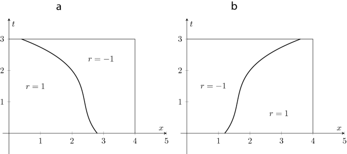
Two possible examples in which \(R' \le 0\)
In this case we write the problem
$$\begin{aligned} \left\{ \begin{array}{ll} (r \, u_{t})_t + {\mathcal {B}}\, u = f &{} \text {in } \Omega \times (0,T) \\ u(x,t) = 0 &{} \text {in } \partial \Omega \times (0,T) \\ u_t(x,0) = \varphi (x) &{} \text {in } \Omega _+(0) \\ u_t(x,T) = \psi (x) &{} \text {in } \Omega _- (T) \\ u(x, 0) = \eta (x) &{} \text {in } \Omega _+(0) \cup \Omega _- (T) \end{array} \right. \end{aligned}$$The operator \(R'(t)\) will be the operator defined as (\(w_1, w_2 \in V = H^1_0 (\Omega )\))
$$\begin{aligned} \big \langle R '(t) w_1 , w_2 \big \rangle _{V' \times V} = \frac{d}{dt} \int _{\Omega } w_1(x) w_2(x) r(x,t) \, dx . \end{aligned}$$We show here a simple example, but for further details we refer to the analogous example in [9] and [8]. In dimension 1 consider r assuming only two values, 1 and \(-1\). Consider then \(\Omega = (a,b)\), \(T > 0\), a function
$$\begin{aligned} \gamma : [0,T] \rightarrow (a,b) , \qquad \gamma \in W^{1,\infty }(0,T) \end{aligned}$$and define the sets
$$\begin{aligned} \omega _+ := \big \{ (x,t) \in \Omega \times (0,T) \, \big | \, x < \gamma (t) \big \} , \qquad \omega _- := \Omega \times (0,T) \setminus \omega _+ \end{aligned}$$(72)and the function r
$$\begin{aligned} r(x,t) = \chi _{\omega _+} (x,t) - \chi _{\omega _+} (x,t) := \left\{ \begin{array}{ll} 1 &{} \text { in } \ \omega _+ \\ -1 &{} \text { in } \ \omega _0 . \end{array} \right. \end{aligned}$$(73)In this case
$$\begin{aligned} \frac{d}{dt} \big ( R(t) w_1 , w_2 \big )_{L^2(a,b)}&= \frac{d}{dt} \int _a^{\gamma (t)} w_1(x) w_2(x) \, dx - \frac{d}{dt} \int _{\gamma (t)}^b w_1(x) w_2(x) \, dx \\&= 2 \, w_1(\gamma (t)) \, w_2(\gamma (t)) \, \gamma '(t) , \end{aligned}$$Then \({\mathcal {R}}'\) turns out to be a non-positive operator if \(\gamma '(t) \leqslant 0\). This situation is shown in Fig. 1a; Fig. 1b shows another possible situation in which \({\mathcal {R}}' \leqslant 0\).
-
10.
One can adapt examples 5 and 7 for the equation \({\displaystyle \int _{\Omega } \big ( r(x,y,t) u_{t} (y,t) \big )_t dy } + {\mathcal {B}}u = f\).

Change history
31 August 2021
A Correction to this paper has been published: https://doi.org/10.1007/s00526-021-02024-3
References
Fichera, G.: Sulle equazioni differenziali lineari ellittico-paraboliche del secondo ordine. Atti Accad. Naz. Lincei Mem. Cl. Sci. Fis. Mat. Natur. Sez. Ia (8) 5, 1–30 (1956)
Germain, P.: The Tricomi equation, its solutions and their applications in fluid dynamics. In: Tricomi’s Ideas and Contemporary Applied Mathematics, Vol. 147 of Accad. Naz. Lincei, Rome, pp. 7–26 (1998)
Glazatov, S.N.: Some nonclassical boundary value problems for linear equations of mixed type. Sibirsk. Mat. Zh. 44, 44–52 (2003)
Keyfitz, B.L.: The Fichera function and nonlinear equations. Rend. Accad. Naz. Sci. XL Mem. Mat. Appl. (5) 30, 83–94 (2006)
Lions, J.L., Magenes, E.: Problemes aux limites non homogenes et applications, vol. 1. Dunod, Paris (1968)
Morawetz, C.S.: Mixed equations and transonic flow. J. Hyperbol. Differ. Equ. 1(1), 1–26 (2004)
Moretti, V.: Spectral Theory and Quantum Mechanics, Vol. 64 of Unitext. Springer, Milan (2013). (With an introduction to the algebraic formulation)
Paronetto, F.: Further existence results for elliptic-parabolic and forward-backward parabolic equations. Calc. Var. Partial Differential Equations 59(4), no. 4, Paper No. 137, pp. 30 (2020)
Paronetto, F.: Existence results for a class of evolution equations of mixed type. J. Funct. Anal. 212(2), 324–356 (2004)
Paronetto, F.: An existence result for a class of second order evolution equations of mixed type. J. Differ. Equ. 226, 525–540 (2006)
Paronetto, F.: \(G\)-convergence of mixed type evolution operators. J. Math. Pures Appl. 9(93), 361–407 (2010)
Paronetto, F.: A Harnack’s inequality for mixed type evolution equations. J. Differ. Equ. 260, 5259–5355 (2016)
Showalter, R.E.: Hilbert Space Methods for Partial Differential Equations. Electronic Monographs in Differential Equations, San Marcos, TX, (1994). iii+242 pp. http://ejde.math.unt.edu/
Showalter, R.E.: Monotone Operators in Banach Space and Nonlinear Partial Differential Equations. American Mathematical Society (1997)
Zeidler, E.: Nonlinear Functional Analysis and its Applications, vol. II A and II B. Springer, New York (1990)
Funding
Open access funding provided by Università degli Studi di Padova within the CRUI-CARE Agreement.
Author information
Authors and Affiliations
Corresponding author
Additional information
Communicated by C. De Lellis.
Publisher's Note
Springer Nature remains neutral with regard to jurisdictional claims in published maps and institutional affiliations.
The original online version of this article was revised: due to change in text and figure caption.
Rights and permissions
Open Access This article is licensed under a Creative Commons Attribution 4.0 International License, which permits use, sharing, adaptation, distribution and reproduction in any medium or format, as long as you give appropriate credit to the original author(s) and the source, provide a link to the Creative Commons licence, and indicate if changes were made. The images or other third party material in this article are included in the article’s Creative Commons licence, unless indicated otherwise in a credit line to the material. If material is not included in the article’s Creative Commons licence and your intended use is not permitted by statutory regulation or exceeds the permitted use, you will need to obtain permission directly from the copyright holder. To view a copy of this licence, visit http://creativecommons.org/licenses/by/4.0/.
