Stacked ResNet-LSTM and CORAL model for multi-site air quality prediction

Abstract

As the global economy is booming, and the industrialization and urbanization are being expedited, particulate matter 2.5 (PM_2.5) turns out to be a major air pollutant jeopardizing public health. Numerous researchers are committed to employing various methods to address the problem of the nonlinear correlation between PM_2.5 concentration and several factors to achieve more effective forecasting. However, a considerable space remains for the improvement of forecasting accuracy, and the problem of missing air pollution data on certain target areas also needs to be solved. Our research work is divided into two parts. First, this study presents a novel stacked ResNet-LSTM model to enhance prediction accuracy for PM_2.5 concentration level forecast. As revealed from the experimental results, the proposed model outperforms other models such as boosting algorithms or general recurrent neural networks, and the advantage of feature extraction through residual network (ResNet) combined with a model stacking strategy is shown. Second, to solve the problem of insufficient air quality and meteorological data on some research areas, this study proposes the use of a correlation alignment (CORAL) method to carry out a prediction on the target area by aligning the second-order statistics between source area and target area. As indicated from the results, this model exhibits a considerable accuracy even in the absence of historical PM_2.5 data in the target forecast area.

1 Introduction

The rapid development of the global economy over the past few years has mostly come at the expense of environmental pollution. As environmental pollution becomes increasingly serious, environmental governance and protection gained rising attention from the public [1]. Inimical health impacts from exposure to outdoor air pollutants refer to complex interaction of pollutant compositions [2, 3]. Real-time air quality information is essential for air pollution inspection and strategic decisions making, which is helpful to protect human health from air pollutants [4]. Atmospheric particulate matter, as a crucial indicator of air quality, deserves to be monitored and predicted. Accurate PM_2.5 forecasting can significantly help in improving prompt and complete environmental quality information, thus allowing the government to take timely action for environmental protection [5]. Besides, the prediction model helps to investigate and study the complicated nonlinear relationship between PM_2.5 and meteorological factors [6].

Several research groups have conducted relevant prediction studies on PM_2.5 or PM₁₀ and other atmospheric pollutants that impair air quality [7]. Moreover, they have employed hidden semi-Markov model [8], support vector machine [9], neural networks [10, 11] and other prediction models trained on historical data. These models have achieved a certain degree of forecasting capability, whereas for hourly forecasts the prediction accuracy must be further improvement. Since for many statistical models it is difficult to capture the complex nonlinear behavior of PM_2.5 concentration change with varying meteorological conditions, more sophisticated models need to be developed that extract features present in meteorological data at a given instant as well as temporal features to follow and consider the trend. In addition, some target locations lack historical data of air quality. However, classical supervised learning methods rely on a large amount of the past data and require observations, i.e. measured data from the target locations, to train the models [12]. To confront this problem, we propose to employ the method of correlation alignment-our second model-that partly overcomes the necessity of historical air quality data.

2 Related work

In comparison with the mature weather forecast, air quality prediction is affected by a variety of complex factors, including climate, traffic, topography, etc., which are extremely complex and nonlinear processes [13]. PM_2.5 concentration prediction methods are mainly divided into two categories: (1) Comprehensive regional scale model based on spatial geographic information and physical/chemical rules. (2) Data-oriented regression prediction model based on machine learning and deep learning algorithm (or models).

As Geographic Information System (GIS) [14], Remote Sensing (RS) [15] and Global Positioning System (GPS) [16] technologies are leaping forward, the PM_2.5 concentration at ground level can be estimated through remote sensing by measuring Aerosol Optical Depth (AOD) [17]. Researchers established a correlation between AOD data and (surface) PM_2.5 concentration to monitor the temporal and spatial distribution of PM_2.5 near the ground [18]. Ma et al. adopted satellite remote sensing to estimate ground-level PM_2.5 and developed a national-scale geographically weighted regression (GWR) model with fused satellite AOD as the principal predictor to forecast diurnal PM_2.5 concentration in China [19]. There are extremely complex physical and chemical reactions and gas-solid two-phase transformation processes between various air pollutants. Some comprehensive regional-scale models can simulate the emission, chemical transformation, and transport of air pollutants, such as NAQPMS, CAMx, and WRF-Chem [20]. Saide et al. proposed an air quality prediction system under the WRF-Chem model, capable of effectively estimating 24-h mean PM_2.5 and PM₁₀ concentrations for 2008 winter in Santiago, Chile [21]. Hong et al. developed a statistical model to optimize the estimation of the initial conditions of aerosol in the WRF-Chem model and improved PM_2.5 forecasting by integrating data from Himawari-8 (a Japanese weather satellite) and ground observations. The experiments were conducted in parallel over eastern China, and results reveal that the model they proposed greatly improved the PM_2.5 predictions [22]. It is worth noting that the performance of this model is highly correlated with the amount of valid data. Comprehensive regional-scale models require satellite remote sensing to obtain continuous and dynamic data on a large scale. The management, analysis, and visualization of massive data greatly increase work costs. Besides, affected by differences in geographic information, this type of model can be only applied to a specific area.

PM_2.5 prediction pertains to time series problems. Classical time series forecasting approaches employ one-dimensional information and analyze changing trends of target value by complying with sequential variations. The representative autoregressive integrated moving average (ARIMA) model [23, 24] has been extensively employed to predict air pollutants concentration. However, the ARIMA model focuses only on historical air quality data, whereas the effect of meteorological factors cannot be considered comprehensively. For this reason, such a method commonly has limited accuracy in PM_2.5 prediction. As compared with general statistical models, applying machine learning algorithms can better address some complex nonlinear relationships between dependent variables, thereby achieving better accuracy in air quality prediction [25]. Zhu et al. proposed an hourly forecast of air pollution concentration (e.g., PM_2.5 and sulfur dioxide) with machine learning approaches. They used refined models to make a prediction based on the meteorological data of previous days instead of applying standard regression models [26]. Since the change of PM_2.5 concentration is affected by many variables, it shows strong nonlinear characteristics. Artificial neural networks have great advantages in solving complex nonlinear problems [27] and also are based on existing monitoring data for modeling, so they have become the research focus of many researchers in the field of air pollution prediction. Wang et al. utilized the Back Propagation (BP) neural network to forecast the PM_2.5 in the Fuling District of Chongqing and the predicted results of this model demonstrated a similar trend with the measured values [28]. Huang et al. proposed the deep learning model APNet based on convolutional neural network (CNN) and long short-term memory (LSTM), which uses the characteristics of CNN to automatically extract features and complete the layer-by-layer abstraction of multiple feature sequences of a single site. Compared with the BP network, the CNN and LSTM network structures and operations are more complicated. The authors showed that this model is capable of predicting the PM_2.5 concentration in the next 1 h more accurately than using CNN or LSTM alone [29]. Yeo et al. proposed a deep learning model which combines a CNN and a gated recurrent unit (GRU) to forecast PM_2.5 concentrations at 25 stations in Seoul, South Korea. In comparison with LSTM, GRU is computationally more efficient and its performance is well-matched as well. According to the average index of agreement, their approach has greatly improved prediction accuracy on the target station [30].

The proposed model in this study is aimed to accurately predict the 6-h PM_2.5 concentration of multiple areas in Beijing and avoid the poor-fitting phenomenon of traditional model at high concentration points. A novel model is built based on ResNet for feature extraction, LSTM for time series analysis and model-stacking technique. Moreover, to address the missing air quality data and meteorological information in the target prediction area, a transfer learning model based on domain adaption is constructed, which maps the data from the source and target domains. The main contributions of this study are as follows:

• 1. This study builds a basic model termed as ResNet-LSTM [31], which uses a ResNet CNN to extract important information from the historical PM_2.5 concentrations and meteorological data. In the experiment, it is shown that after the feature extraction from ResNet, the prediction accuracy can be improved. In the low concentration range of PM_2.5 (≤ 75 µg/m³), ResNet-LSTM has a better fitting performance than general recurrent neural networks. The average root-mean-square error, mean absolute error and R-Squared of the ResNet-LSTM model are 44.886 µg/m³, 25.946 µg/m³ and 0.760, respectively.

• 2. To more effectively enhance the forecasting capability of the single model, an ensemble learning method termed as stacking is adopted to combine several basic models. As verified in the comparative experiments, the proposed stacked ResNet-LSTM model outperforms the single basic model when adopted to the test dataset, especially when the observed PM_2.5 values are at a high concentration (≥ 150 µg/m³). The average root-mean-square error (40.679  µg/m³), mean absolute error (23.746 µg/m³) and R-Squared (0.804) verify the feasibility of the stacked ResNet-LSTM model. This stacked model can be used to create an early warning system for high PM_2.5 concentrations.

• 3. To address the lack of historical air quality and meteorological data in some target prediction areas, this study also proposes a domain adaptation method termed as correlation alignment to achieve the PM_2.5 concentration forecasting on these areas. This method can be used as a supplement to the stacked ResNet-LSTM model in the absence of a large amount of historical data at other areas of interest.

3 Data sources

The research city of this study is Beijing, which is the political and economic center of China. The original data used in this study consist of two types, air quality data and meteorological data. Hourly PM_2.5 concentrations (µg/m³) were collected from the Beijing Municipal Environment Monitoring Center (BMEMC). The air quality monitoring sites in the dataset are located in 10 different locations in Beijing. The location, latitude, and longitude of these stations are shown in Table 1. These air quality monitoring stations are distributed in various areas in the city center and suburbs of Beijing, as presented in Fig. 1.

Table 1 Locations of air quality monitoring stations in Beijing

Original meteorological information including temperature ($^{\circ }$C), pressure (hPa), dew point temperature ($^{\circ }$C), wind direction and wind speed ($\mathrm m/s$) were collected from observing stations of the China Meteorological Administration (CMA). The meteorological station is located close to the air monitoring stations in Beijing. On the whole, the combined historical PM_2.5 and meteorological dataset have over 35,000 h of samples from March 1, 2013, to February 28, 2017. Each monitoring point has a dataset of over 35,000 samples.

Fig. 1

Geographical distribution map of Beijing Air Quality Monitoring Stations

3.1 Data pre-processing

Historical monitoring data collected from air quality monitoring stations and meteorological stations face several problems (e.g. missing data and inappropriate data formats). Thus, the original data are preprocessed according to the input requirements of the model for training samples.

The wind direction from original data is expressed in discrete string form, such as “east wind”, “southeast wind”, “northeast wind”. Here, we use a Label Encoding method for the numerical coding of the discrete feature. The 16 different wind directions is coded from 1 to 16. There are few missing data for features such as temperature, air pressure, wind direction, and wind speed (missing meteorological information ranging from 0.3 of to 0.8 % per station), and but those are not the main factors affecting the future changes of PM_2.5 concentration (missing PM_2.5 ranging from 1.1 of to 2.6 % per station). Accordingly, the “backfill” function in Pandas is employed to fill the missing data of these features. Based on the data information of other complete features, the missing PM_2.5 concentration value can be filled with a simple random forest model.

In total, the dataset provides 1461 days of hourly data for air quality and meteorological parameters. In this study, the meteorological data and PM_2.5 data of the first 5 days were chosen as the input feature of the neural network, and the PM_2.5 data of the first 6 h of the sixth day were treated as the corresponding labels, which corresponds to a forecast of 6 h into the future. However, through this method to separate the dataset, the final prediction result of the proposed model is not continuous. To increase the amount of data and make the final prediction output result continuous, a method termed as sliding window was used in this study. By using this mechanism, a high-dimension temporal feature can be constructed for improving the prediction accuracy. Figure 2 illustrates the sliding window method.

Fig. 2

Sliding window method

The feature window consists of the historical meteorological data and air quality data from the past 120 h. The label window includes the following 6 h PM_2.5 concentration data. Every moving step of this mechanism is 6 h, which ensures that the PM_2.5 concentration value for a complete day can be predicted. After the data are processed by using the sliding window method, a total of about 5800 samples are obtained. In the model training process, 69% of the samples in the dataset are employed for training, 17% for validation, as well as 14% for testing. Table 2 lists the distribution of the complete dataset.

Table 2 The distribution of the complete dataset

4 Methods

Based on air quality data and meteorological information in Beijing, this study proposes a data-driven ensemble learning model termed stacked ResNet-LSTM. The PM_2.5 prediction model combines a convolutional neural network (ResNet) that learns local abstract features and a recurrent neural network (LSTM) with long-term memory function, to extract the temporal features of Beijing air quality and weather data. On that basis, an ensemble learning method is adopted to integrate multiple basic models to further enhance the prediction performance of the model. This happens through a stacking method of the separately trained basic models.

To address the missing historical air quality and meteorological data in some target prediction areas, this study also proposes to utilize a domain adaptation method termed as correlation alignment (CORAL) to achieve a forecast of PM_2.5 concentration on different target areas. The entire modeling and training process of the stacked ResNet-LSTM model and the CORAL model is shown in Fig. 3.

Fig. 3

Flowchart of the Stacked ResNet-LSTM model and the CORAL model

4.1 Stacked ResNet-LSTM model

Before integrating several basic models by using an ensemble learning strategy, a basic model termed as ResNet-LSTM needs to be constructed. The architecture of our ResNet-LSTM basic model is shown in Fig. 4. The input of the ResNet-LSTM model is the data of the PM_2.5 concentration, temperature, pressure, dew point temperature, wind speed, and wind direction over the last five days, a total of 120 h as described in Sect. 3.1. The corresponding labels are the PM_2.5 concentration of the following 6 h. The proposed model can be divided into three main parts, namely ResNet for local feature extraction in PM_2.5 and meteorological data, LSTM for temporal dimension extracted features analysis, and fully connected layers for final regression prediction of PM_2.5 concentrations. The basic prediction model ResNet-LSTM is a 37-layer deep network and consists of the following three parts:

Fig. 4

ResNet-LSTM model structure

• (1) ResNet ResNet as a classical convolutional neural network is formulated by a series of basic blocks called residual blocks which can learn the desired mapping by utilizing a special’ shortcut connection’ architecture [32]. As shown in Fig. 5, a desired underlying mapping H(x) is fitted by two stacked nonlinear layers while the skip connection or identity mapping is implemented in the basic block to skip the transformation F(x) to form residual learning. As an alternative to learning a mapping of H(x), the network learns a residual mapping based on the residual function F(x). The ResNet model employed in this study is ResNet-34. Its structure of ResNet-34 is shown in Fig. 6. Since the fully connected layer is removed, it is a 33-layer convolutional neural network.

• (2) LSTMs LSTM refers to an optimized version of recurrent neural network, suitable for processing and predicting important events with relatively long intervals and delays in time series [33]. Our basic model comprises 2 LSTM layers, building a stacked LSTM architecture. The configuration of a LSTM cell consists of three parameters: $batch\_size$, $time\_step$ and $input\_size$. The batch size of LSTM is identical to that of the entire model, which is set to 50 in advance. In the stacked LSTM part of the model, the time step of LSTM is set to 1, indicating that the length of the characteristic sequence processed at one time is 1. The parameter $input\_size$ is set to 64, which means the length of a set of feature sequences is 64. In the 2-layer LSTM, each LSTM layer outputs a sequence of vectors used as an input to a subsequent LSTM layer. This hierarchy of hidden layers enables a more complex representation of our time-series data, so information at different scales is captured.

• (3) Dense The third part of our model consists of two fully connected (dense) layers. Based on a linear activation function, the basic model outputs the predicted PM_2.5 concentration on the target Beijing monitoring station area for the next 6 h.

Fig. 5

Residual block [32]

Fig. 6

ResNet-34 [32]

The dimensional transformation of input features in the proposed network is presented in Fig. 7. After data pre-processing, the input is reshaped into a $120\times 6\times 1$ matrix. The matrix shape originates from 120 h (5 days) of input data with 6 features used (PM_2.5, temperature, pressure, dew point temperature, wind speed, and wind direction); furthermore, the matrix is expanded into the third dimension to be suitable for convolutional operations. Passing through the ResNet CNN, the shape of the input matrix is changed to $15\times 1\times 512$. The subsequent LSTM layers extract and process temporal features. Lastly, the data are sent to multiple fully connected layers to generate forecasting results. The successive layers and the corresponding output shape are listed in Table 3.

Fig. 7

Dimension transformation in ResNet-LSTM model

Table 3 Successive layers and output shape of our suggested model ResNet-LSTM

We employ the mean squared error (MSE) as loss function and optimize the model by adopting AdaDelta optimizer with a learning rate of 1e–4 [34]. The basic model is trained for 300 epochs, and a batch size of 50 is used. For different monitoring stations, the corresponding pre-processed data are adopted to train the basic models. To expedite the convergence of the model and reduce overfitting, several optimization methods (e.g. Dropout, Regularization and EarlyStopping) are adopted. The operation of dropout is to randomly set some neurons in the hidden layer to 0 in accordance with a certain ratio. By exploiting the dropout strategy, the model is forced to learn more robust features and lower the impact of noise. Dropout was applied to the first layer and second layer of the stacked LSTMs part to enable its ability to generalize.

Moreover, the EarlyStopping method in the model is to prevent overfitting and expedite the completion of training. Before the experiments, we need to decide when to stop training according to the current validation result. For instance a decrease in training loss, but increase in validation loss suggests the beginning of overfitting. In this scenario, the training will be stopped automatically. The parameters of Earlystopping are set to $patience=30$, $restore\_best\_weights=True$, which tells how many epochs can be tolerated without model improvement (= decrease in training and validation loss) and that the weight values of the model in its optimal state will be saved.

A 5-fold validation method was adopted to train each basic model with its corresponding dataset. Then, a meta-model (stacked ResNet-LSTM) was constructed through a stacked generalization strategy. Stacked generalization was firstly proposed by David H. Wolpert in 1992 [35], which is an ensemble method that utilizes a high-level model to integrate several base models to achieve better performance in different machine learning tasks such as classification and regression. k-fold cross-validation is used on each base model to avoid the occurrence of overfitting and the ability of the model to generalize.

Considering the expected performances of the basic models and weighting the contribution of each sub-model to the combined prediction can improve the average performance of the model significantly. The modeling process of the stacked ResNet-LSTM model is demonstrated in Fig. 8.

Each single ResNet-LSTM model is treated as a sub-model, and the linear regression acts as a meta-learning machine to construct a stacked ResNet-LSTM model. The specific implementation is as follows:

• Step 1. First spilt the original samples into training dataset M1 and test dataset N1.

• Step 2. Train each level 0 base model on the training dataset and test them on the test dataset (5-fold cross-validation is utilized on each base model).

• Step 3. Use predictions of validation dataset as inputs and corresponding target values to form a new training dataset M2 which is used to train the level 1 meta-model (linear regression here).

• Step 4. Average the predictions of the test dataset N1 to compose a new test dataset N2, and make a final prediction on the meta-model.

  Fig. 8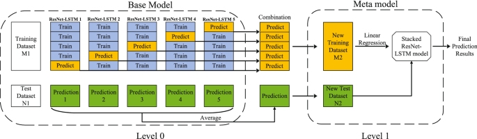

  

  ResNet-LSTM models stacking process

4.2 CORAL PM_2.5 regression model

In order to address the data shortage problem of historical air quality data in the target prediction area, our study adopts a transfer learning method. By aligning the second-order statistics between source domain (auxiliary prediction area) and target domain (target prediction area), a novel transfer learning method termed as CORrelation ALignment (CORAL) is adopted to develop an accurate and effective forecasting model that can be transferred to another prediction area.

4.2.1 Correlation alignment

CORAL refers to a classic statistical transfer learning method by complying with statistical feature transformation. The basic principle of the statistical feature alignment method is to transform and align the second-order statistics (covariance) between source domain and target domain [36]. The aligned covariances can be learned by adopting traditional machine learning methods to develop a classifier. The main application of the CORAL model is image classification. In the proposed model, however, after the source domain and target domain data are aligned, a KNN regression algorithm can be adopted to predict the PM_2.5 concentrations on the target domain.

Suppose a labeled source domain dataset $D_\mathrm{s}=\{x_i\}^{n_\mathrm{s}}_{i=1}$, $x\in R^{d}$ with labels $L_\mathrm{s}=\{y_i\}^{n_\mathrm{s}}_{i=1}$, and an unlabeled target domain dataset $D_\mathrm{t}=\{u_j\}^{n_\mathrm{t}}_{j=1}$, $u\in R^{d}$, where $n_\mathrm{s}$ and $n_\mathrm{t}$ are the number of samples in source domain and target domain respectively. Both x and u are the d-dimensional feature representations. The correlation alignment method aligns the two domains with second-order features. Assuming that $C_{rm s}$ and $C_{rm t}$ are the covariance matrices of the source domain and the target domain, it learns a second-order feature transformation A that minimizes the feature distance between the source domain and the target domain.

$$\begin{aligned} \min \limits _{A}\left\| C_{\hat{s}}-C_\mathrm{t}\right\| _{F}^{2}=\min \limits _{A}\left\| A^{\mathsf {T}}C_\mathrm{s}A-C_\mathrm{t}\right\| _{F}^{2}, \end{aligned}$$

(1)

where $C_{\hat{s}}$ represents the covariance matrix after the correlation alignment, A is the matrix for linear transformation. $\left\| \cdot \right\| _{F}^{2}$ represents the matrix Frobenius norm.

By solving the above optimization objective, the transformation matrix A can be obtained. The specific derivation process is explained in the “Appendix”.

4.2.2 K-Nearest Neighbor regression

The K-Nearest Neighbor (KNN) regression algorithm refers to an example-based learning method, with the core idea to build a vector space model. By exploiting a certain distance measurement method, this algorithm aims at finding the neighbor points in the training set that are the nearest to the test point, and then employing the neighbor points to predict the test set. The average output of the neighboring points acts as the prediction result.

After the optimal A linear transformation matrix is generated by using the CORAL method, A can be utilized with the original source domain data to generate new source domain features. The KNN algorithm is then employed to build a regression model according to the procedure mentioned before. The input of this regression model is the newly generated (or transformed) features of the source domain, and the corresponding labels refer to the original labels from source domain. Then, the target domain features are given into the KNN regression model to obtain the corresponding labels to the target domain, which is the actual regression prediction result.

Fig. 9

Idea of CORAL PM_2.5 regression model

Fig. 10

Sliding window of CORAL PM_2.5 regression model

The training and prediction process of the CORAL PM_2.5 model is shown in Fig. 9. Here, we use 150 source domain samples and 150 target domain samples for training. 120 h of PM_2.5 concentration, temperature, pressure, and other features are also used as the input of one sample and the corresponding label in the source domain is the PM_2.5 concentration of the following 6 h. A sliding window mechanism is also utilized for the training and prediction of the CORAL PM_2.5 regression model. As shown in Fig. 10, a sliding window named CORAL window is composed of a source domain window and a target domain window. A source domain window and a target domain window include 150 samples respectively as mentioned before. After aligning the covariances between the input of the source domain and target domain, a KNN regression model is trained based on the transformed features of the source domain and their corresponding labels, which is then applied to the target domain to generate prediction results. Keeping the result of the last sample, the sliding window moves forward by one sample.

5 Simulation analysis

5.1 Evaluation metrics

Three evaluation metrics are adopted to evaluate the experimental results, which are root-mean-squared error ($\mathrm RMSE$), mean absolute error ($\mathrm MAE$), as well as R-Squared ($R^2$). The RMSE is the arithmetic square root of the mean squared error, which is employed to measure the deviation between the real value and the predicted value. The MAE indicates the average absolute error between the observed value and predicted value. Smaller RMSE and MAE represent better model performance. The values of R-squared ranges from 0 to 1; the closer to 1, the better the fitting results of the model will be. The formulas of the three metrics are written as follows:

$$\begin{aligned} \mathrm{RMSE}&=\sqrt{\frac{1}{n}\sum _{i=1}^{n}\left( y_i-\hat{y}_{i}\right) ^2} \end{aligned}$$

(2)

$$\begin{aligned} \mathrm{MAE}&=\frac{1}{n}\sum _{i=1}^{n}\left| y_i-\hat{y}_{i} \right| \end{aligned}$$

(3)

$$\begin{aligned} R^2&=\frac{\sum _{i}\left( \hat{y}_{i}-\overline{y}\right) ^2}{\sum _{i}\left( y_{i}-\overline{y}\right) ^2}, \end{aligned}$$

(4)

where $y_{i}$, $\hat{y}_{i}$ and $\overline{y}$ represent true value, prediction value and mean value.

5.2 Methods for comparison

The proposed models are compared with the following methods:

• (1) Gradient Boosted Decision Tree (GBDT) GBDT is a gradient boosting of weak learners using CART (Classification and Regression Tree) [37]. One characteristic of using a decision tree as a weak learner is that the decision tree itself is an unstable learner, indicating that a slight fluctuation of the training data may significantly impact the results. From a statistical perspective, the variance of a single decision tree is relatively large. In ensemble learning, however, the larger the variance between the weak learners, the better the generalization performance of the weak learners, and ultimately of the entire ensemble learning model.

• (2) LightGBM It refers to Microsoft’s open-source distributed high-performance gradient boosting framework, which applies a learning algorithm based on decision trees [38]. LightGBM adopts a histogram-based decision tree algorithm to discretize continuous floating-point eigenvalues into k integers and construct a histogram with a width of k. It abandons the level-wise decision tree growth strategy followed by GBDT and uses a leaf-wise strategy with depth restrictions, which is a more efficient tree growth strategy compared to level-wise. On each step, it identifies the leaf with the largest split gain among all current leaves, then splits. Accordingly, compared with level-wise, leaf-wise is capable of reducing more errors and achieving better accuracy in the identical number of splits.

• (3) Long short-term memory (LSTM) As a type of recurrent neural network, it is also capable of learning order dependence in time-series prediction problems [39].

• (4) Gated recurrent unit (GRU) GRU is a further developed version of the standard recurrent neural network, i.e., a variant of LSTM. As compared with LSTM, the construction of GRU is simpler since it is reduced by one gate, and matrix multiplication is less strained. GRU involves fewer parameters than LSTM, so it exhibits a faster training speed and requires fewer samples. Nevertheless, if training data is enough, the test performance of LSTM may be better than GRU because LSTM has more flexibility when it comes to writing, reading and flushing the cell. As a variant of LSTM, GRU combines the input gate and the forget gate in LSTM into one, termed as “Update Gate”, which controls the amount of data that the previous memory information continues to retain to the current moment. Further, as there is no hidden memory state M in the GRU as opposed to the LSTM, the GRU’s update gate additionally acts as the output gate in the LSTM [40].

• (5) ResNet-LSTM As a basic model, ResNet-LSTM can also be used in time series forecasting.

• (6) Transfer component analysis (TCA) As a kind of transfer learning algorithm, TCA is proposed to solve domain adaption problems by learning a shared subspace by minimizing the dissimilarities across domains [41]. (1), (2), (3), (4), (5) will act as the comparison algorithms in comparative experiments with stacked ResNet-LSTM, and (5), (6) will be used in comparative experiments with transfer learning model CORAL.

In the comparative experiments, 300 iterations are performed for the respective neural network model and utilized the stochastic gradient descent technique for training. Moreover, the number of batches is set to 50, the value of learning rate is 1e–4, the number of LSTM/GRU units (dimensionality of the output space) is set to 64. Specific to boosting algorithms and TCA, the optimal parameters of the mentioned models are found with the grid search method. The specific parameter settings are listed in Table 4.

Table 4 Model parameter settings

5.3 Result analysis

5.3.1 Comparative experiments of stacked ResNet-LSTM

Tables 5, 6 and 7 list the three evaluation metrics of the stacked ResNet-LSTM model and its comparative models at 10 air quality monitoring stations in Beijing.

The proposed model stacked ResNet-LSTM shows its prominent performance in accordance with the three evaluation indexes. As is shown in Fig. 11, the average RMSE (40.679), MAE (23.746) generated by the proposed model are the lowest among all the models and its $R^2$ (0.804) is also the highest. It is therefore demonstrated that the proposed model stacked ResNet-LSTM exhibits significantly better universality in different target prediction areas to achieve high accuracy forecasting as compared with other algorithms. Since ResNet exhibits an outstanding ability of feature extraction and stacking generalization could further enhance forecasting ability, the stacked ResNet-LSTM model has thus better prediction performance compared with boosting algorithms and general neural network models. As indicated in Fig. 11, the classic recurrent neural network LSTM has a slightly better prediction performance than its variant GRU according to the average values of the three metrics. This is probably because LSTM has a better model expression performance than GRU under the abundant training samples in the training dataset.

Table 5 The experimental results in terms of RMSE

Table 6 The experimental results in terms of MAE

Table 7 The experimental results in terms of R-Squared

With the location Nongzhanguan (#6) as an example, Fig. 12 illustrates the scatter plots of actual observed PM_2.5 values and corresponding prediction results generated by each model. The areas exhibiting high scatter plot density of LSTM and GRU are slightly concentrated above the 1:1 line, i.e., the predicted PM_2.5 is significantly higher than the real value when the observed PM_2.5 is at a low concentration. Figure 13 presents the forecast result for 1000 h from 2016-12-10 to 2017-01-20 in Huairou as a time series, where the black line refers to the observed values, the other colored lines are the prediction results of each model. The analysis of the prediction results and comparison to the observations suggests that classical boosting algorithms and neural network models can effectively track the future changing trend of PM_2.5 concentration values. According to Fig. 13, there is a significant deviation in the prediction results of LSTM (Green line) and GRU (Pink line), when the PM_2.5 pollution concentration is relatively low.

Fig. 11

The comparison of average RMSE, MAE and R-Squared between Stacked ResNet-LSTM and other comparative models

Fig. 12

Scatter density graph for observed and predicted PM_2.5 values between Stacked ResNet-LSTM and other comparative models for location Nongzhanguan. The redder the color, the denser the scatter

Fig. 13

Prediction results of different models and their comparison

To more effectively analyze the forecasting results under different observed values, the air quality is classified according to PM_2.5 concentration levels as given as follows:

• 1. Good PM_2.5 does not exceed 75 µg/m³

• 2. Mild or moderate pollution PM_2.5 is between 75 µg/m³ and 150 µg/m³

• 3. Severe pollution PM_2.5 is greater than 150 µg/m³

The red, orange, and green boxes in Fig. 13 present the detailed comparison results of the respective model under the mentioned three air quality situations. According to the green box, the prediction results of LSTM and GRU present a cyclical fluctuation state when the observed PM_2.5 values are lower than 75 µg/m³. However, this phenomenon occurs only very slightly in the ResNet-LSTM model. Compared with LSTM and GRU, the prediction of the ResNet-LSTM model fits the observed PM_2.5 value to a higher extent. It is therefore inferred that for recurrent neural networks, feature extraction operation is capable of effectively avoiding model failure under low concentration prediction. Among all the models, the performance of GBDT, LightGBM, ResNet-LSTM and stacked ResNet-LSTM is best when air quality is in good condition. However, it is still noteworthy that most algorithms cannot comply with the real trend when it increases rapidly in a short period. Furthermore, as indicated from this phenomenon, great difficulties remain in accurately predicting PM_2.5 changes. The yellow box presents the comparison results of each model under mild or moderate pollution. It can be seen that the prediction result of the LightGBM model (orange line) has three obvious spikes, which is far from the actual observed values. The other models are capable of predicting the changing trend of PM_2.5 in this concentration range to a better extent. The red box presents the results of each model when the PM_2.5 concentration value exceeds 150 µg/m³. As already revealed from the green box, the prediction results of LSTM, GRU and ResNet-LSTM show periodic oscillations, which demonstrates that they cannot achieve accurate forecasting under severe pollution. Nevertheless, after the basic model is integrated, the ensemble model stacked ResNet-LSTM effectively avoids the mentioned phenomenon and demonstrates better nonlinear fitting ability even at high pollution levels.

5.3.2 Comparative experiments of the CORAL model

In this study, three locations, i.e., Aotizhongxin (#1), Dongsi (#4) and Wanliu (#9), are taken as research objects (Fig. 14). In the respective experiment, two of the three above locations are selected as experimental objects to compare the prediction results between the transfer learning methods and the ResNet-LSTM basic model. Different from the transfer learning models, ResNet-LSTM model directly used the training dataset from the target prediction area for training.

Fig. 14

Experimental locations of the transfer learning model. The tail of the arrow represents the source domain. The head of the arrow represents the target domain

Table 8 Results of comparative experiments for different models compared to the CORAL model at three different locations, Huairou, Aotizhongxin, and Changping

Table 8 lists the result statistics of all comparative experiments. According to three evaluation metrics, the performance of the ResNet-LSTM model is the optimal generally, followed by CORAL and TCA last. This is not surprising since ResNet-LSTM-as a supervised learning model-is capable of training a model with high prediction accuracy given sufficient training data. In the actual use-case of our underlying assumption (not sufficient training data available in target area), the ResNet-LSTM model could not be trained and therefore would not exist, but in our experiment we do have the training data and therefore can provide the ResNet-LSTM metrics for a comparative analysis with our CORAL and TCA results. In several cases (e.g. Aotizhongxin as the source domain and Wanliu as the target domain), the R-squared value of the CORAL model prediction result reaches 0.715, close to the ResNet-LSTM model prediction result of 0.763. The forecasting results of Aotizhongxin as target domain and Wanliu as source domain are taken as an example for illustration in Fig. 15. As revealed from the scatter density graph, the prediction results of CORAL at low concentrations are more concentrated on the 1:1 line in comparison to ResNet-LSTM, although ResNet-LSTM has better performance according to the evaluation indicators. The fitting curves of different models in Aotizhongxin are plotted in Fig. 16. According to those, all models are capable of basically tracking changes of PM_2.5 concentration. At some individual time points, the prediction results of the CORAL model and the TCA model show large deviations. But in relation to the training data from the source domain, they already give a relatively accurate forecast performance.

Fig. 15

Scatter density graph for observed and predicted PM_2.5 values between the CORAL model and other comparative models

Fig. 16

Prediction results of the CORAL model and comparative models

As suggested from the mentioned three sets of comparative experiments, the ResNet-LSTM air quality prediction model is the optimal under sufficient experimental data in the target domain. However, for insufficient experimental data in the target domain, using transfer learning methods is considered to be more effective. In some specific scenarios, the prediction results of the CORAL method by adopting source domain data for training are significantly close to the supervised learning model ResNet-LSTM (e.g., transferring from Aotizhongxin to Wanliu). For the comparison of the two transfer learning methods, the CORAL method results outperform those achieved by using the TCA method, independent of which source domain and target domain are combined. Lastly, when building a transfer learning model for the target domain, a suitable source domain should be selected, thereby positively impacting the prediction results [42]. Here, we use the CORAL loss as a metric of the distance between the second-order statistics of the source and target features [43].

$$\begin{aligned} \ell _\mathrm{CORAL}=\frac{1}{4d^2}\left\| C_\mathrm{s}-C_\mathrm{t}\right\| _{F}^{2}, \end{aligned}$$

(5)

where d represents the dimension of the feature.

Table 9 presents the CORAL loss between three different domains. It can be seen from Table 9 that the CORAL loss between Aotizhongxin and Wanliu is the smallest (1098.699), and as is shown in Table 8, the three evaluation metrics between these two domains are also the best in the comparative experiments. Besides, if choosing Wanliu as the target domain, Aotizhongxin-which has a smaller CORAL loss with Wanliu than Dongsi with Wanliu-performs better in the transfer learning prediction. Taking into account the analyses above, we can come to the conclusion that the smaller CORAL loss, the better prediction performance. When utilizing transfer learning to make a prediction on a target area, it is preferred to choose the location with the smallest CORAL loss as the source domain.

Table 9 CORAL loss between three domains

6 Conclusion

In order to take air pollution forecasting accuracy to the next level, this study constructed an ensemble deep neural network prediction model–the stacked ResNet-LSTM model. In this article, we use ResNet to process the high-dimensional data to forecast the PM_2.5 concentration 6 h into the future based on historical air quality data and meteorological information. The novel network architecture enables us to explore time-related features and statistical features and provides an accurate prediction on the future PM_2.5 concentration. Moreover, an ensemble method is utilized to increase the prediction accuracy. With PM_2.5 and meteorology data from Beijing, a care study has been performed to verify the superiority of the proposed model. To be specific, the stacked ResNet-LSTM model outperforms the other individual models in all prediction areas of our case study in Beijing, achieving a maximal average R-squared value of 0.804 followed by ResNet-LSTM (0.760), LightGBM (0.754), GBDT (0.751), LSTM (0.715), as well as GRU (0.706). The other evaluation metrics RMSE and MAE of stacked ResNet-LSTM are the lowest among all the comparative models, which indicates a better performance. For the stacked ResNet-LSTM model, its practicality and generalization for forecasting the PM_2.5 concentration are verified here.

Furthermore, to solve the problem of data deficit for PM_2.5 prediction in areas of interest with insufficient data availability, this study employed a domain adaptation-based model, termed as CORAL. This model is capable of effectively improving PM_2.5 prediction in data shortage scenarios, and its experimental performance is significantly close to the supervised learning model ResNet-LSTM in several scenarios. It is noteworthy that it is also critical to select a suitable location as the source domain of the CORAL model, which can significantly improve the forecasting results of the target predicted area.

Nowadays, deep learning models are also facing privacy and security issues. The most representative existing privacy threats include model extraction attacks and model inversion attacks [44]. A model inversion attack uses APIs (Application Programming Interfaces) provided by the machine learning system to obtain preliminary information of the model and performs reverse analysis on the model through those preliminary information to further obtain private data inside the model or to even reconstruct training data samples [45]. In a model extraction attack, an attacker infers the parameters or functions of the model by sending data in a loop and observing the model results, thereby replicating a machine learning model with similar or even identical functions [46]. In the future, we would like to investigate some privacy-preserving technologies and integrate them into our proposed models to protect the training data and model parameters from hacking.

Appendix

In this chapter, the process of deriving the linear transformation matrix A as used in Sect. 4.2.1 is shown in detail.

Conducting the singular value decomposition (SVD) on $C_\mathrm{s}$ and $C_\mathrm{t}$, thus $C_\mathrm{s}=U_\mathrm{s}\varSigma _\mathrm{s}U_\mathrm{s}^{\mathsf {T}}$ and $C_\mathrm{t}=U_\mathrm{t}\varSigma _\mathrm{t}U_\mathrm{t}^{\mathsf {T}}$ can be obtained, where $U_\mathrm{s}$ is a left singular vector, $U_\mathrm{s}^{\mathsf {T}}$ is a right singular vector, and $\varSigma _\mathrm{s}$ is the diagonal matrix of singular values. The optimal solution to Eq. 1 is as follows:

$$\begin{aligned} C_{\hat{s}}=U_{\mathrm{t}[1:r]}\varSigma _{\mathrm{t}[1:r]}U_{\mathrm{t}[1:r]}^{\mathsf {T}}, \end{aligned}$$

(6)

where $r=\mathrm{min}(r_{C_\mathrm{s}},r_{C_\mathrm{t}})$. Let $C_{\hat{s}}=A^{\mathsf {T}}C_\mathrm{s}A$:

$$\begin{aligned} A^{\mathsf {T}}C_sA=U_{t[1:r]}\varSigma _{\mathrm{t}[1:r]}U_{\mathrm{t}[1:r]}^{\mathsf {T}}, \end{aligned}$$

(7)

where the diagonal elements of $\varSigma _{t[1:r]}$ are r largest singular values, the columns of $U_{\mathrm{t}[1:r]}$ are the corresponding left-singular vectors and the rows of $U_{t[1:r]}^{\mathsf {T}}$ are the corresponding right-singular vectors. Because $C_\mathrm{s}=U_\mathrm{s}\varSigma _\mathrm{s}U_\mathrm{s}^{\mathsf {T}}$, Eq. 7 can be rewritten as:

$$\begin{aligned} A^{\mathsf {T}}U_\mathrm{s}\varSigma _\mathrm{s}U_\mathrm{s}^{\mathsf {T}}A=U_{\mathrm{t}[1:r]}\varSigma _{\mathrm{t}[1:r]}U_{\mathrm{t}[1:r]}^{\mathsf {T}}. \end{aligned}$$

(8)

Then, it gives:

$$\begin{aligned} \left( U_\mathrm{s}^{\mathsf {T}}A\right) ^{\mathsf {T}}\varSigma _{s}\left( U_\mathrm{s}^{\mathsf {T}}A\right) =U_{\mathrm{t}[1:r]}\varSigma _{\mathrm{t}[1:r]}U_{\mathrm{t}[1:r]}^{\mathsf {T}}. \end{aligned}$$

(9)

Let $E=\varSigma _\mathrm{s}^{+\frac{1}{2}}U_\mathrm{s}^{\mathsf {T}}U_{\mathrm{t}[1:r]}\varSigma _{\mathrm{t}[1:r]}^{\frac{1}{2}}U_{\mathrm{t}[1:r]}^{\mathsf {T}}$, where E is the Moore–Penrose pseudoinverse of $\varSigma _\mathrm{s}^{+\frac{1}{2}}$. Then the right hand side of Eq. 9 can be written as follows:

$$\begin{aligned} \left( U_\mathrm{s}^{\mathsf {T}}A\right) ^{\mathsf {T}}\varSigma _\mathrm{s}\left( U_\mathrm{s}^{\mathsf {T}}A\right) =E^{\mathsf {T}}\varSigma _\mathrm{s}E. \end{aligned}$$

(10)

Lastly, the optimal solution of A is yielded.

$$\begin{aligned} A=U_\mathrm{s}E=\left( U_\mathrm{s}\varSigma _\mathrm{s}^{+\frac{1}{2}}U_\mathrm{s}^{\mathsf {T}}\right) \left( U_{\mathrm{t}[1:r]}\varSigma _{\mathrm{t}[1:r]}^{\frac{1}{2}}U_{\mathrm{t}[1:r]}^{\mathsf {T}}\right) . \end{aligned}$$

(11)

References

Kostka G, Nahm J (2017) Central-local relations: recentralization and environmental governance in china. China Q 231:567–582
Curtis L, Rea W, Smith-Willis P, Fenyves E, Pan Y (2006) Adverse health effects of outdoor air pollutants. Environ Int 32(6):815–830
Leikauf GD, Kim SH, Jang AS (2020) Mechanisms of ultrafine particle-induced respiratory health effects. Exp Mol Med 52(3):329–337
Wang X, Wang B (2019) Research on prediction of environmental aerosol and PM2.5 based on artificial neural network. Neural Comput Appl 31(12):8217–8227
Zhang B, Zhang H, Zhao G, Lian J (2020) Constructing a PM2.5 concentration prediction model by combining auto-encoder with bi-lstm neural networks. Environ Model Softw 124:104600
Tao G, Chen H, Li W (2020) Beijing PM2.5 influencing factors analysis based on gam. In: 2020 IEEE/WIC/ACM International Joint Conference on web intelligence and intelligent agent technology (WI-IAT), IEEE, p 916–921
Iskandaryan D, Ramos F, Trilles S (2020) Air quality prediction in smart cities using machine learning technologies based on sensor data: a review. Appl Sci 10(7):2401
Dong M, Yang D, Kuang Y, He D, Erdal S, Kenski D (2009) PM2.5 concentration prediction using hidden semi-markov model-based times series data mining. Expert Syst Appl 36(5):9046–9055
Dong Y, Wang H, Zhang L, Zhang K (2016) An improved model for PM2.5 inference based on support vector machine. In: 2016 17th IEEE/ACIS International Conference on software engineering, artificial intelligence, networking and parallel/distributed computing (SNPD), IEEE, p 27–31
Fu M, Wang W, Le Z, Khorram MS (2015) Prediction of particular matter concentrations by developed feed-forward neural network with rolling mechanism and gray model. Neural Comput Appl 26(8):1789–1797
Chen Y (2018) Prediction algorithm of PM2.5 mass concentration based on adaptive bp neural network. Computing 100(8):825–838
Xie H, Ji L, Wang Q, Jia Z (2019) Research of PM2.5 prediction system based on cnns-gru in Wuxi urban area. In: IOP Conference series: earth and environmental science. IOP Publishing, vol 300, p 032073
Singh KP, Gupta S, Kumar A, Shukla SP (2012) Linear and nonlinear modeling approaches for urban air quality prediction. Sci Total Environ 426:244–255
Foresman TW (1998) The history of geographic information systems: perspectives from the pioneers, vol 397. Prentice Hall PTR, Upper Saddle River
Campbell JB, Wynne RH (2011) Introduction to remote sensing. Guilford Press
Enge PK (1994) The global positioning system: Signals, measurements, and performance. Int J Wirel Inf Netw 1(2):83–105
Wang J, Christopher SA (2003) Intercomparison between satellite-derived aerosol optical thickness and PM2.5 mass: Implications for air quality studies. Geophys Res Lett 30(21)
Han X, Cui X, Ding L, Li Z (2019) Establishment of PM2.5 prediction model based on MAIAC AOD data of high resolution remote sensing images. Int J Pattern Recognit Artif Intell 33(03):1954009
Ma Z, Hu X, Huang L, Bi J, Liu Y (2014) Estimating ground-level PM2.5 in china using satellite remote sensing. Environ Sci Technol 48(13):7436–7444
Xi X, Wei Z, Xiaoguang R, Yijie W, Xinxin B, Wenjun Y, Jin D (2015) A comprehensive evaluation of air pollution prediction improvement by a machine learning method. In: 2015 IEEE International Conference on service operations and logistics, and informatics (SOLI), IEEE, pp 176–181
Saide PE, Carmichael GR, Spak SN, Gallardo L, Osses AE, Mena-Carrasco MA, Pagowski M (2011) Forecasting urban PM10 and PM2.5 pollution episodes in very stable nocturnal conditions and complex terrain using wrf-chem co tracer model. Atmos Environ 45(16):2769–2780
Hong J, Mao F, Min Q, Pan Z, Wang W, Zhang T, Gong W (2020) Improved PM2.5 predictions of wrf-chem via the integration of Himawari-8 satellite data and ground observations. Environ Pollut 263:114451
Wang W, Guo Y (2009) Air pollution PM2.5 data analysis in los angeles long beach with seasonal Arima model. In: 2009 International Conference on energy and environment technology, IEEE, vol 3, pp 7–10
Zhang L, Lin J, Qiu R, Hu X, Zhang H, Chen Q, Tan H, Lin D, Wang J (2018) Trend analysis and forecast of PM2.5 in Fuzhou, china using the Arima model. Ecol Ind 95:702–710
Deters JK, Zalakeviciute R, Gonz´alez M, Rybarczyk Y (2017) Modeling PM2.5 urban pollution using machine learning and selected meteorological parameters. J Electr Comput Eng 2017:5106045:1–5106045:14
Zhu D, Cai C, Yang T, Zhou X (2018) A machine learning approach for air quality prediction: Model regularization and optimization. Big Data Cogn comput 2(1):5
Li S, Li Y (2013) Nonlinearly activated neural network for solving time-varying complex Sylvester equation. IEEE Trans Cybern 44(8):1397–1407
Wang X, Yuan J, Wang B (2021) Prediction and analysis of PM2.5 in fulling district of Chongqing by artificial neural network. Neural Comput Appl 33(2):517–524
Huang CJ, Kuo PH (2018) A deep cnn-lstm model for particulate matter (PM2.5) forecasting in smart cities. Sensors 18(7):2220
Yeo I, Choi Y, Lops Y, Sayeed A (2021) Efficient PM2.5 forecasting using geographical correlation based on integrated deep learning algorithms. Neural Comput Appl 33(22):15073–15089
Choi H, Ryu S, Kim H (2018) Short-term load forecasting based on resnet and lstm. In: 2018 IEEE International Conference on Communications, Control, and Computing Technologies for Smart Grids (SmartGridComm), IEEE, pp 1–6
He K, Zhang X, Ren S, Sun J (2016) Deep residual learning for image recognition. In: Proceedings of the IEEE Conference on computer vision and pattern recognition, pp 770–778
Hochreiter S, Schmidhuber J (1997) Long short-term memory. Neural Comput 9(8):1735–1780
Zeiler MD (2012) Adadelta: an adaptive learning rate method. arXiv preprint arXiv:1212.5701
Wolpert DH (1992) Stacked generalization. Neural Netw 5(2):241–259
Sun B, Feng J, Saenko K (2017) Correlation alignment for unsupervised domain adaptation. In: Csurka G (ed) Domain adaptation in computer vision applications. Springer, pp 153–171
Friedman JH (2001) Greedy function approximation: a gradient boosting machine. Ann Stat 29(5):1189–1232
Ke G, Meng Q, Finley T, Wang T, Chen W, Ma W, Ye Q, Liu TY (2017) Lightgbm: a highly efficient gradient boosting decision tree. In: Guyon I, Luxburg UV, Bengio S, Wallach H, Fergus R, Vishwanathan S, Garnett R (eds) Advances in neural information processing systems, Curran Associates, Inc., pp 3146–3154
Zhang W, Wang L, Chen J, Xiao W, Bi X (2021) A novel gas recognition and concentration detection algorithm for artificial olfaction. IEEE Trans Instrum Meas 70:1–14
Cho K, Van Merriënboer B, Gulcehre C, Bahdanau D, Bougares F, Schwenk H, Bengio Y (2014) Learning phrase representations using rnn encoder-decoder for statistical machine translation. arXiv preprint arXiv:1406.1078
Pan SJ, Tsang IW, Kwok JT, Yang Q (2010) Domain adaptation via transfer component analysis. IEEE Trans Neural Netw 22(2):199–210
Bascol K, Emonet R, Fromont E (2019) Improving domain adaptation by source selection. In: 2019 IEEE International Conference on Image Processing (ICIP), pp 3043–3047
Sun B, Saenko K (2016) Deep coral: correlation alignment for deep domain adaptation. In: European Conference on computer vision, Springer, pp 443–450
Liu X, Xie L, Wang Y, Zou J, Xiong J, Ying Z, Vasilakos AV (2020) Privacy and security issues in deep learning: a survey. IEEE Access 9:4566–4593
Fredrikson M, Jha S, Ristenpart T (2015) Model inversion attacks that exploit confidence information and basic countermeasures. In: Proceedings of the 22nd ACM SIGSAC Conference on computer and communications security, pp 1322–1333
Tramèr F, Zhang F, Juels A, Reiter MK, Ristenpart T (2016) Stealing machine learning models via prediction apis. In: 25th USENIX Security Symposium (USENIX Security 16), pp 601–618
Acknowledgements
This work was supported by the Professorship of Environmental Sensing and Modeling grant funded by the German Research Foundation (DFG) under Grant Nr. 419317138.
Funding
Open Access funding enabled and organized by Projekt DEAL.
Author information
Authors and Affiliations
Corresponding authors
Ethics declarations
Conflict of interest
The authors declare that they have no known competing financial interests or personal relationships that could have appeared to influence the work reported in this paper.
Additional information
Publisher's Note
Springer Nature remains neutral with regard to jurisdictional claims in published maps and institutional affiliations.