Arabic text classification: the need for multi-labeling systems

Abstract

The process of tagging a given text or document with suitable labels is known as text categorization or classification. The aim of this work is to automatically tag a news article based on its vocabulary features. To accomplish this objective, 2 large datasets have been constructed from various Arabic news portals. The first dataset contains of 90k single-labeled articles from 4 domains (Business, Middle East, Technology and Sports). The second dataset has over 290 k multi-tagged articles. To examine the single-label dataset, we employed an array of ten shallow learning classifiers. Furthermore, we added an ensemble model that adopts the majority-voting technique of all studied classifiers. The performance of the classifiers on the first dataset ranged between 87.7% (AdaBoost) and 97.9% (SVM). Analyzing some of the misclassified articles confirmed the need for a multi-label opposed to single-label categorization for better classification results. For the second dataset, we tested both shallow learning and deep learning multi-labeling approaches. A custom accuracy metric, designed for the multi-labeling task, has been developed for performance evaluation along with hamming loss metric. Firstly, we used classifiers that were compatible with multi-labeling tasks such as Logistic Regression and XGBoost, by wrapping each in a OneVsRest classifier. XGBoost gave the higher accuracy, scoring 84.7%, while Logistic Regression scored 81.3%. Secondly, ten neural networks were constructed (CNN, CLSTM, LSTM, BILSTM, GRU, CGRU, BIGRU, HANGRU, CRF-BILSTM and HANLSTM). CGRU proved to be the best multi-labeling classifier scoring an accuracy of 94.85%, higher than the rest of the classifies.

1 Introduction

Large numbers of repositories live online as a result of the heavy usage of Web 2.0 and the Internet, which leads to a need and demand for automatic classification methods. Almost 80% of data is textual and unstructured but considered an extremely valuable and rich source of information. Machine learning algorithms have been proved helpful in cutting the time needed to extract insights and organize massive chunks of data.

One of the fundamental tasks in natural language processing (NLP) is text classification. It is used to assign labels to textual data based on its context. Automating the process simplifies classifying documents, helps in standardizing the platform, and makes searching for specific information straightforward and possible.

Manually classifying documents by experts is not as efficient as it used to be due to their increasing amount. This is where machine learning algorithms come into play, as an alternative to conventional ways. They produce faster and more fruitful results. Several examples and applications of text classification have been explored such as language identification [38], dialect identification [19], sentiment analysis  [16, 17, 22,23,24] and spam filtering [2, 37].

Structuring data using machine learning are becoming essential in the business field. It helps in detecting new patterns and trends and identifies relationships between seemingly unrelated data. For example, marketers can gather and review keywords used by other firms in the field. For Arabic NLP, this is still a challenging task among others [29]. It is a very complex, morphological-derived language, and it is the mother tongue of over 300M people. The research done in the field of Arabic computational linguistics is impressively increasing in the last decade, but the work still has room to expand and branch out.

Arabic has been reported by the Internet World Stats to be the 4th most popular language online, with over 225k users, representing 5.2% of all Internet users as of April 2019. They also show that it has the highest growth rate in the number of users in the last 19 years, achieving 8,917.3%.

Working with Arabic text is different from working with English text. It is more challenging for several reasons which include the following: (1) Forms: Arabic has three different forms (Classical, Modern Standard Arabic (MSA), and Dialectal), (2) Vocabulary size: Arabic language has around 12.3 million words compared to 600,000 words in English, (3) Alphabet set: the character set has 28 consonants and 8 vowels. Besides, when writing cursive script several characters have different shape-forms. The Arabic text is written from right to left, (4) Grammar: Arabic assigns words, verbs, and pronouns to a gender. It also has singular and plural forms for both male and female. Further, conjugated verbs in Arabic are different, (5) Vowels: a significant difference is in the quality and length of the vowels. Arabic generally uses diphthongs and long vowels as in-fixes, and (6) Sentence structure: Arabic has verbal and nominal sentences. A nominal sentence does not require a verb.

In this work, we first introduce a newly built single-labeled dataset of Arabic news articles, collected from several portals to aid our research. Several classifier models are trained to predict the single class a proposed article belongs to. Moreover, a voting classifier has been implemented, considering the best predicting classifiers, with the highest accuracy percentage.

An Arabic news article single-labeling classification excerpts from text the linguistic features using the TF-IDF technique. In the training phase, each article is turned into a feature vector, and then, the system identifies the most common features under each category. This way, when the classifier encounters a new article, it will attempt at predicting the relevant category based on its features vectors.

We propose a multi-class classifier, to label an Arabic news articles under an appropriate class out of 4 classes. We used a supervised approach for text classification. We tested different vectorization methods to seek the best, and to see the effect they have on the accuracy percentages. In addition, we investigated the possibility of using a customized list of stop words as a replacement for using the NLTK list.

Looking at the misclassified articles by the classifying system, we decide to construct a new Arabic multi-labeled dataset for the purpose of assigning the articles to multi-labels instead. Two approaches were tested. Firstly, we implemented two classical classifiers made compatible with the task of multi-labeling. Second, we built ten neural networks with unique architectures to test the effectiveness of deep learning techniques. For the first approach, we used the TF-IDF technique for feature extract. Both classifiers need to be wrapped in a OneVsRest Classifier, to convert the classification problem to sub-problems. For the second approach, we used the tokenizer provided by Keras before training.

We offer a multi-label multi-class text categorization system that is capable at assigning an article with multiple labels out of 21 labels. We evaluate and compare the two approaches using the custom accuracy metric specific to the multi-labeling system, along with hamming-loss scores. This work is an extension of our work [4, 5] on single-label classification.

To summarize, in this work, we propose two new large datasets for Arabic news articles tagging. One dataset is dedicated for single-label classification, while the other dataset is dedicated for multi-label classification. Both datasets are new to the Arabic computational linguistics field and shall serve the need for such rich datasets. Furthermore, we demonstrate the validity and efficacy of these proposed datasets by studying the performance of several shallow as well as deep learning models to classify Arabic text. This is a comprehensive study on the task of Arabic news classification, which is needed to fill this research gap. In conclusion, the contributions of the work are:

• Two large Arabic datasets, which tat are comprised of news articles spanning several topics, are properly annotated for Arabic text classification. The datasets shall be made available for researchers in the Arabic natural language processing field.

• A rigorous investigation of several shallow and deep learning classification models is carried out for the Arabic text classification task to choose the best models.

• Considerable experiments are conducted to confirm the fitness of the proposed datasets and the classification models.

• Fine-tuning of the models as well as the utilization of word embedding is performed to achieve solid performance.

The paper is organized as follows: The literature review is presented in Section 2. Section 3 demonstrates the dataset. Sections 4 and 5 detail the proposed classification process. The results and discussion are presented in Sect. 6. At last, we present our conclusions in Sect. 7.

2 Literature review

Many surveys and papers shed light on the different approaches used for English text categorization and discuss existing literature [1, 18, 36]. For Arabic text classification, surveys like [7, 33] also exist. Some researchers investigated the classification task on other languages such as Portuguese. In [28], they used an SVM classifier on an English dataset and on a Portuguese dataset. They found that the Portuguese language required paying more attention to the document representation like semantic/syntactic information and word order.

Arabic text classification research and the goal to enrich the Arabic corpus are slowly becoming a priority in the research community. In [31], the authors believe that many of the available datasets are not appropriate for classification, either because the classes are not defined well, or there are not any defined classes like in the 1.5 billion words Arabic Corpus [11]. The authors also introduce 'NADA,' a new filtered and preprocessed corpus, that combine already existing corpora DAA and OSAC. 'NADA' contains 13,066 documents belonging to 10 categories in total. With regard to the number of labels, we believe that the corpus is too small.

Recent research papers focusing more on Arabic text classification (ATC) are emerging. The author in [20] used a dataset of articles collected from (aljazeera.com), to compare the performance of 6 different classifiers. Under the same environmental settings, Naive Bayes was the best classifier, regardless of feature selection methods.

Many papers experiment with feature selection methods. In [8], they studied the effect of using uni-grams and bi-grams, experimenting with the KNN classifier. In [39], they reported that using an SVM classifier, for ATC, outperforms other classifiers. An experiment on 4 classifiers while by means of 2 feature selection techniques (information gain and chi-squared) was conducted on a BBC Arabic dataset in [41]. Lastly, in [31], the authors present a new feature selection method for ATC, and it outperforms five other approaches, testing them using the SVM classifier.

Many authors reported results of supervised classical machine learning algorithms such as NB [12, 14, 21, 40], SVM [3, 12, 27, 32], Decision Tree [3, 30, 42], KNN [14, 32].

Several others preferred to work with deep learning techniques and experimented with neural networks like in [9, 10, 15, 25] to tackle the single-label classification problem. Authors pursuing better results using a different approach such as [15] have used a convolution neural network for Arabic text classification and achieved better results than Logistic Regression and SVM. In [10], the authors proved that using feature reduction techniques with an ANN model achieves higher results than a basic ANN model. An extended work to address the multi-labeling classification task using a variety of deep learning models is studied in [26]. In this work, we show a more comprehensive study by including classical machine learning algorithms, which produce superb results as well.

All the above references worked on the single-labeling task of Arabic text. Nonetheless, the need for integrating multi-labeling is becoming essential. A vast set of news article span more than one major topic. For example, a news article that talks about covid-19 (medical domain) and its impact on the economy should be tagged with both labels rather than only one. Multi-labeling would resolve the intersection of multiple domains instead of just selecting one. In fact, more electronic news portals are tagging each news article with multiple tags (keywords). This process is usually carried out by humans. Therefore, the need for an automated tagging system is becoming a necessity. While multi-labeling task is well researched for the English language (for example, see [13, 44]), it is under-researched for Arabic language. This work helps to bridge this gap in the Arabic computational linguistic field. In the sequel, we describe few studies on this task for Arabic.

Shehab et al. [43] investigated the multi-label classification task using three machine learning classifiers, which are Decision Trees (DT), Rain Forest (RF), and KNN. The results show that DT outperforms the other 2 classifiers. This is a limited study; there are more robust classifiers that can outperform DT as we show in our work. Hmeidi et al. [34] used a lexicon-based system to classify Arabic documents. The dataset has 8,800 multi-label documents collected from BBC Arabic. Several single-label and multi-label lexicons were produced to tackle the problem. The dataset is relatively small to handle effectively multi-label tagging. Besides, scalability is a major concern with lexicon-based methods. Both of these works used hamming loss metric as an evaluating metric, along with precision and recall.

Al-Salemi et al. [6] proposed a new dataset gathered from RT-news (RTANews) website for multi-labeling of Arabic news articles. They explored 4 transformation-based algorithms: Binary Relevance, Classifier Chains, Calibrated Ranking by Pairwise Comparison and Label Powerset. They used 3 classifiers, namely SVM, KNN, and RF. They reported that RF and SVM produced the best results. However, the dataset has $87\%$ of the documents was tagged with a single label. As a result, the dataset is biased toward single-label rather than multi-label classification. This shortcoming would heavily impact the performance of the proposed algorithms on another balanced dataset.

It is clear that the accuracy and the general performance are highly dependable on the quality of the collected data and by the feature representation method. The more redundant features we have, the less accurate the classification is. Therefore, we introduce new rich and representative datasets for treating the problem of both single-label and multi-label Arabic documents classification. We truly believe that the datasets would serve as benchmarks. In contrast with the existing research works on this task, we provide a thorough examination of several shallow and deep learning algorithms to robustly solve the automatic tagging of Arabic news articles.

3 Datasets

We visited 7 popular news portals (arabic.rt.com, youm7.com, cnbcarabia.com, beinsports.com, arabic.cnn.com, skynewsarabic.com and tech-wd.com), to collect the articles from. We used (Python Scrapy) library to scrape the articles. The single labeled dataset contains 89,189 Arabic documents (approximately 32.5 million words). The articles of the dataset are categorized under four main classes: [’Sports,’ ’Middle East politics,’ ’Business’ and ’Technology’].

All the collected articles are written in Modern Standard Arabic (MSA), with no dialects. The articles are grouped in one corpus.

Table 1 Number or documents collected from 7 news portals

Fig. 1

Some statistics on the single-label dataset categories

Table 1 and Fig. 1 describe the distribution of the articles under the 4 categories in the dataset. In average, we scraped around 22k articles for each category. We made sure to avoid bias by constructing a balanced dataset.

Table 2 Scraped news portal for the multi-label dataset

Fig. 2

Some statistics on the multi-label dataset categories

As for the multi-label dataset, we collected this dataset using (Python Scrapy, Selenium and BeautifulSoup) from ten different websites listed in Table 2. The articles in this dataset, all belong to one of the 4 classes: [Middle East, Business, Technology, Sports], in additional to hundreds of tags. It consists of 293,363 multi-tagged articles written in (MSA). Figure2 shows the distribution of the articles in the main categories.

4 Single-label classification

4.1 Text features

Machine learning algorithms cannot process text directly, and to solve this, we represent the text in numerical vectors. Words of the articles represent categorical features, and each sentence will be presented by one vector. This process is called vectorization. Two of the most common techniques used in text vectorization are countVectorizer and TF-IDFVectorizer. Both of these vectorizers are used to represent textual data in vector format. While countVectorizer keeps track of the number of tokens (i.e., features) encountered in a document, TF-IDFVectorizer stores the weighted frequency of each token with respect to the document. TF-IDFVectorizer is favored over countVectorizer as the latter one is biased to most frequent tokens opposed to low frequent features that may be key feature in determining the document genre. To overcome this problem, we adopted TF-IDFVectorizer, which will compute the relative frequency of each feature in each document. This vectorizer computes the most common features which could identify the document main topics. However, as it is based on the bag-of-words (BoW) concept, it does not capture the semantics when compared to other models such as word embeddings. We conducted an experimental comparison between the two vectorizer methods. We used a subset of our single-labeled dataset, containing 40k articles, classified under three categories. The comparison involves using each vectorizer as the features selection technique, which shall be fed to the same classifier (SVM) to determine the document genre (single-label) for all documents in the dataset. Table 3 confirms that higher accuracy scores were produced when using the TF-IDF vectorizer as opposed to the countVectorizer.

Table 3 TF-IDF vectorizer versus count vectorizer: performance evaluation

Fig. 3

Generic system flow-diagram

Tokens that appear very frequently have a less of an impact when being represented by the term frequency-inverse document frequency. This vectorizer is made up of two components:

• Term Frequency (TF): computes how many times a word appears in a given document, then adjusts the frequency taking into consideration the length of the document.

• Inverse Document Frequency (IDF): computes how common or rare a word is in the entire article set. If a word appears many times and is common, the score approaches 0, otherwise, it approaches 1.

After that, we conducted another comparison using a custom-made list of stop-words instead of the built-in list. In fact, we adopted the customized list as it reported better results. The general flow of operations of the proposed system is described in Fig. 3.

4.2 Selected classifiers

Several different supervised classifiers are used for text classification, where the main purpose is to tag an input text with the best representative label. We studied and observed the performance of ten shallow learning models, in addition to the ensemble classifier. Next, we describe all implemented algorithms:

• Logistic Regression (LR): this is a predictive model. It is a statistical learning technique used for the task of classification. Even though the name of the classifier has the word ‘Regression’ in it, it is used to produce discrete binary outputs.

• Multinomial Naïve Bayes (MNB): this classifier estimates the probability of each class-label, based on Bayes theorem, for some text. The result is the class-label with the highest probability score. MNB assumes the features are independent, and as a result, all features contribute equally to the computation of the predicted label.

• Decision Tree (DT): DT is basically a tree, where nodes represent features and leaves are the output labels. Branches indicate decisions and whenever a decision is answered, a new decision will be inserted recursively until a conclusion is made. Recursion is used to partition the tree into several decisions with possible results.

• Support Vector Machines (SVM): SVM is a very prevalent supervised classifier. It is non-probabilistic. SVM uses hyperplanes to segregate labels. SVM supports linear and nonlinear models. Basically, each hyperplane is expressed by the input documents (vector) x satisfying $w\dot{x}-b= 0$, where w is the normal vector to the hyperplane, and b is the bias.

• Random Forest (RF): RF is a supervised learning-based classifier. This ensemble model utilizes a set of decision trees, which computes the resulting label aggregately. Strictly, the input is the documents $x_1,x_2,\dots ,x_n$ with their matching labels $y_1,y_2,\dots ,y_n$. Each decision tree $f_b$ is trained using a random sample $(X_b,Y_b)$, where b ranges from 1 to the total number of trees. The forecasted label shall be computed by a majority vote of all used trees.

• XGBoost Classifiers (XGB): XGB is another supervised classifier. This robust classifier became popular as a result of winning several Kaggle contests. Similar to RF, it is an ensemble classifier made of decision trees and a variant of the gradient boosting algorithm.

• Multi-layer Perceptron (MLP) Classifier: MLP is comprised of at least 3 layers of neuron nodes (input layer, hidden layers, and output layer). As for general neural networks, each node is connected to nodes in the subsequent layer. MLP utilizes a non-linear activation function to produce the resulting label.

• KNeighbors Classifier (KNN): KNN classifier determines the neighbors of an input document. The predicted class label is collectively computed by all determined neighbors, where each one votes for the closest label. The class-label with the maximum ballots is adopted. This is another major vote classifier.

• Nearest Centroid Classifier (NC): for NC, the class-label is the centroid of its data points. Given an input document then the class-label is computed based on the training examples whose mean (centroid) is closest to the input document.

• AdaBoost Classifier (ADB): ADB is a meta-estimator that starts by fitting a classifier on the training set of documents. Next, AB fits additional copies of the classifier on the training dataset but after adjusting the weights of misclassified documents such that succeeding classifiers attend to problematic cases¹.

• Ensemble/Voting Classifier (VC): VC is basically an ensemble solution. VC is packaging all preceding classifiers. Majority voting is utilized for predicting the final class label.

5 Multi-label classification systems

5.1 Classical classifiers

We selected 2 classical classifiers: [OneVsRestLogisticRegression, and OneVsRestXGBoost]. The OneVsRest Classifier decomposes the multi-label problem into multiple independent binary classification problems (one per label). Both LogisticRegression classifier and XGBoost classifier were each wrapped inside a OneVsRestClassifier. We used the TF-IDF technique to vectorize the articles, and we chose to keep the default hyperparameters for each classifier. To encode the labels, we used MultiLabelBinarizer() that returns the string labels assigned to each article in a one-hot encoded format.

5.2 Deep learning classifiers

Artificial neural networks are computational models that are designed to behave similarly to the functionality of a human brain from analyzing information to deciding actions. They are implemented to solve problems that are impossible or hard to solve by human or mathematical standards. Traditionally, a neural network consists of plenty of nodes that work in parallel with each other, consisting of a layer. These layers are then connected to make up the network. Deep neural networks are neural networks with different numbers of layers between both layers, the input layer and the output layer. These additional layers are called hidden layers. Their main objective is to add more computation to the network to solve complicated tasks. These three main layers are connected to form a DNN model. These networks can be tweaked to perform well on images, audio and textual data.

In our work, we use each of convolution neural networks and recurrent neural networks models for the multi-labeled text classification. Overall, we designed ten different models. These models are described below.

Convolution neural networks (CNN) are unique classes of neural network models that are designed to identify hidden patterns and relationships in large data sets. The role of CNNs is to learn different features utilizing many filters. These features are then taken down further to learn high-order features. CNN uses a pooling layer which is main function is to reduce the spatial dimensions by performing downsampling. Applying a max-pooling layer with filters of size 2x2 is the most common approach in pooling. Here, we perform a pooling operation that returns the maximum value on a window of size 2x2. Another type called average-pooling works similar to the mentioned type above however, this will return only the average value instead.

Recurrent neural networks (RNN) RNN models are more powerful in use cases in which context and time are critical. Backpropagation enables looping information back through the network which empowers RNN models with processing sequential data. This helps finding correlations between dependent variables. In our work, we combine CNN and RNN to generate a new CRNN architecture. The new architecture applies a spatial dropout for the embedding layer, we then have a Conv1D layer followed by an RNN layer, we then add a global max pooling layer followed by a dropout layer to apply regularization. Finally, we have a dense layer followed by the output layer. Next, we describe the most common models of RNN.

Long short-term memory (LSTM) can be constructed by using a number of LSTM units to make up the network. They are applicable for different tasks that require sequential data such as text classification and time series forecasting. This is different from RNN since they can remember longer sequences for long periods of time. LSTM has three types of gates: the input, the output gates and the update gates. These gates determine what data to keep and what data to throw away.

Gated Recurrent Unit (GRU), although both units tackle the vanishing gradient problem, GRUs are distinguished from LSTMs by possessing a hidden state (memory). GRU utilizes 2 gates: an update gate and reset gate. The reset gate determines the amount of past information to forget, while the update gate decides what information to keep and what to not.

Hierarchical Attention Network (HAN) is extremely good at predicting the class of a given document, because it recognizes its structure. A document is constructed by first encoding the words, then encoding the sentences to form a document representation. An attention mechanism is also used in a HAN, to make sure that the context of a word or a sentence is accounted for. Words and sentences also differ in importance in regard to the main message of the document.

5.3 Proposed deep learning models

In our work, we developed ten deep learning models. We experimented the combination of both CNN and RNN in addition to CRF-CNN have been used to develop many models on different tasks. These new approaches have shown better results compared to the traditional machine learning models.

Each of these models is composed of an input embedding layer, multi hidden layers, and a dense output layer. The utilization of embedding layer helps in capture the semantic relationships between words and so it assigns similar words similar representations.

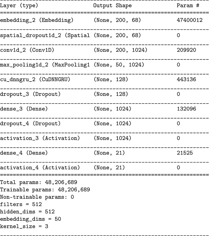
An embedding layer is internally used to convert a sparse one-hot encoded matrix to a dense vector space. This reduces the computational complexity and so the training time. A word2vec word embedding was first trained on our dataset and used in our experiment; however, it was producing poor results. Thus, we ditched it and kept using the Keras tokenizer. The size of the input is set to 200 words, and this was obtained by trying different sizes. We then design different types of deep neural network and use the best design in our work.

For the last dense layer, which is the output layer, we want multi-labels as an output, so we use a binary crossentropy loss function along with the sigmoid activation function. Its output dimension is equal to the number of categories available.

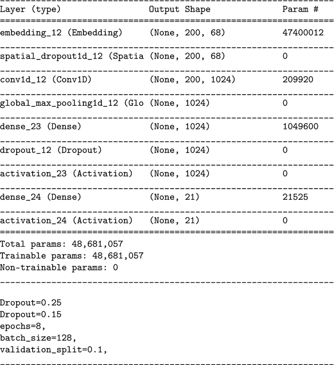
• CNN: The CNN model consists of a spatial dropout layer, followed by one CNN layer with kernel size of 3, and 1024 filters, followed by a global max pool layer and a dropout layer.

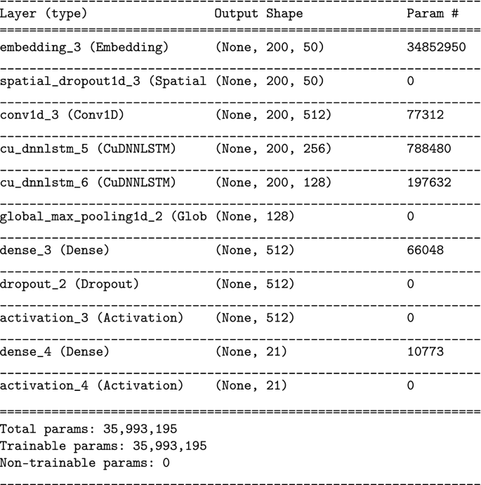
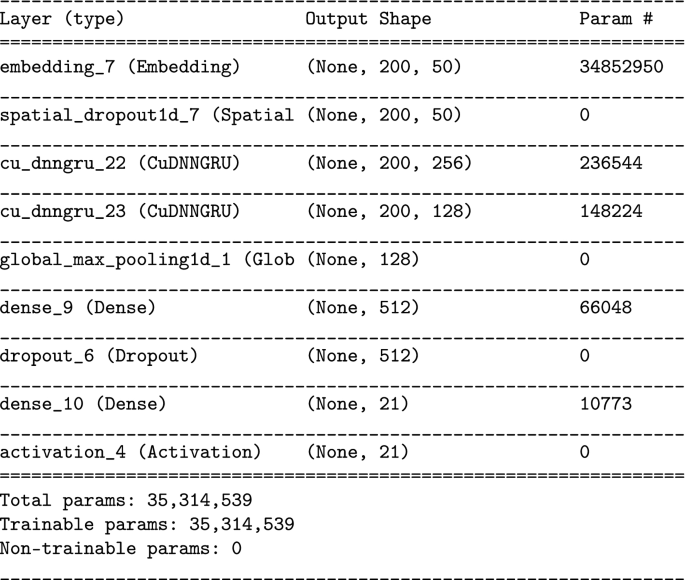
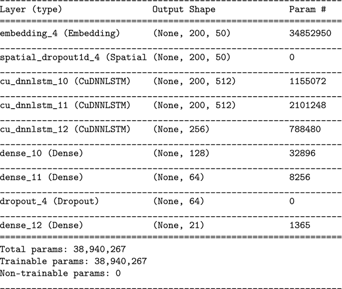
• RNN: We used both LSTM and GRU models. The LSTM model consists of three layers, while the GRU model consists of four layers. These selections have been carefully chosen by testing different implementations of these models, we then picked the methods that were giving best accuracies. Both models are improved versions of standard RNN, which solve the vanishing gradient problem.

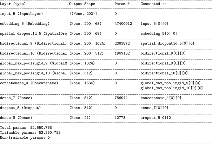
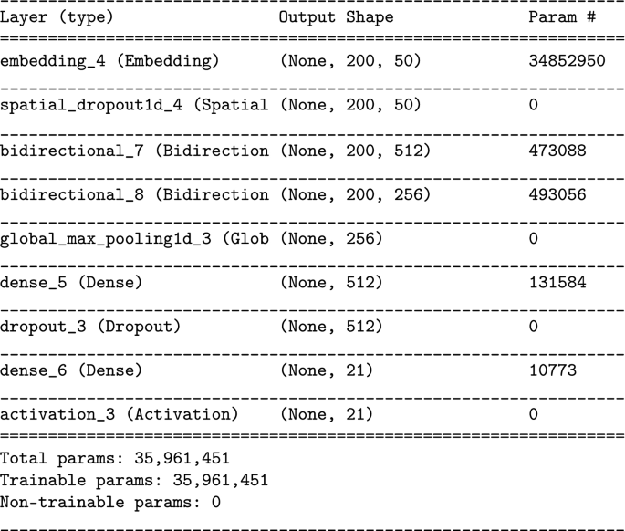
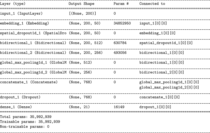
• BIRNN: For an enhanced performance on sequence classification problems, both RNN models are wrapped by a Bidirectional wrapper. The data are fed to the learning algorithm once from the beginning to the end, and once in reverse. Running the input bidirectionally will result in the network understanding the context better. In the forward run, both LSTM and GRU preserve information from the past, and in the backward run, future information is preserved.

• Bi-LSLTM - CRF: Adding a CRF layer to a bidirectional neural network has been proven to be very effective for sequence labeling tasks. Since the CRF model is a unidirectional model, providing the sequence in both directions will decrease the ambiguity of the words in the sequence.

• CNN + RNN: We generate a new CRNN architecture by combining each of CNN and RNN layers together. The new architecture applies a spatial dropout for the embedding layer, we then have a Conv1D layer followed by an RNN layer, we then add a global max pooling layer followed by a dropout layer to apply regularization. Finally, we have a dense layer followed by the output layer.

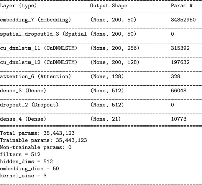
• HAN: Applying an additional layer after the RNNs models, called attention layer. Along with solving the long-term memory issues with RNNs, the output sequence generated will be conditional on selective items in the input sequence. The hierarchical attention network is extremely good at predicting the class of a given document, because it recognizes its structure. A document is constructed by first encoding the words, then encoding the sentences to form a document representation. An attention mechanism is also used in a HAN, to make sure that the context of a word or a sentence is accounted for. Words and sentences also differ in importance in regards to the main message of the document.

6 Experimental results and discussion

6.1 Single-label classification

The objective is to put 11 classifying models to the test and determine how successful they are to single-label Arabic news articles. We will perform single-label classification on a subset of our single-labeled dataset. After that we will compare the performance of the same models on a recently reported Arabic dataset ‘Akhbarona’ [25, 26] that contains seven categories in total. In this experiment, we used the 80% for training, 20% for testing split. The training set consists of 71,707 articles, while the testing set contained 17,432 articles.

We calculate the accuracy score to evaluate the performance of the classifiers. The accuracy score is the total number of correctly classified samples over the total number of samples. From the training set, we extracted about 344 k features. Additionally, pre-processing of input documents is performed in order to remove all the non-Arabic characters. When dealing with textual data collect from the web, it is highly advised to use this method. We proceed further by cleaning the scraped articles and erasing all the elongation, digits, punctuation, isolated chars, Latin letters, Qur’anic symbols, and other marks that were possibly included.

Fig. 4

Performance of all classifiers on our proposed dataset

We believe that applying normalization on the collected text is not a necessary step, even though majority of research works on Arabic NLP tasks do implement normalization. There are enough samples provided in the dataset to represent Arabic character-set. It is worth noting that in some cases, the normalization step can change the semantics of some words. Normalization, which is a widely adopted practice in Arabic computational linguistics, is the process of unifying the orthography of some Arabic characters. Namely, alif forms [ا ، أ ، إ ، آ ] to [ا ] , hamza forms [ئ، ؤ، ء ] to [ء ] , haa/taa marbootah [ه، ة] to [ه ] , and yaa/alif maqsura [ى، ي ] to [ى ] . The normalization step is meant to reduce the vocabulary space. However, this process may lead to losing some key features as the meaning of some words would change after normalization. For example, the word “فأر” (means “mouse”) while “فار” after normalization means 'escaped' or 'كرة,', which means 'football,' after normalization becomes “كره” , which means “hatred”. Such meaning-change could result in dropping some important features. In addition, with a large corpus such as the ones proposed in this work, there is no need for this pre-processing step. In fact, the results show that the non-normalized word representation is not seriously hampered by the lack of text normalization.

To implement the classifiers, we used Scikit-learn and kept using the default hyper-parameters in addition to L1 penalty for some of the models. We used the testing set to test the proposed classifiers. The high accuracy scores indicate how robust the proposed system is based on the tuned hyper-parameters.

Figure 4 demonstrates the accuracy scores that were obtained by the classifiers. 94.8% was the average of the accuracy score. The best result, 97.9%, was achieved by the SVM classifier. On the other hand, the worst result, which is 87.7%, was produced by the AdaBoost classifier. Furthermore, close results that range from 97.5% to 97.9% were produced by four classifiers.

Fig. 5

The confusion matrices for highest(SVM) and lowest (AD) performers

Table 4 Evaluation metrics for all classifiers on the testing dataset

The two classifiers, MultinomialNB and KNeighbors, produced the accuracies of 96.3% and 95.4%, respectively, meanwhile the remaining classifiers produced scores that range from 87.7% to 94.4%, which is below the average compared to the previous classifiers. Figures 5 displays the confusion matrix for the best and worst classifiers, which are SVM and AdaBoost, respectively.

Furthermore, Table 4 states that SVM scored the highest F1-score 98%, similar to the majority voting classifier, while the lowest score of 88% was produced by the AdaBoost classifier. We also include ROC, Hamming score, F1-score, precision, and recall metrics. We demonstrate the robustness of the best classifier, SVM, by showing the results of prediction. Figure 6 shows an article, from the testing set, which is originally tagged as ‘Technology’. SVM model was able to classify the article under the same category, with an accuracy of 95.7%. We examined a sample of the incorrectly classified documents from the testing dataset in order to recognize the reason behind the misclassification. We realized that several documents can be argued as incorrectly classified. Figure 7 shows an article that was initially classified under ‘Technology.’ After reading the article, we concluded that it belongs to the ‘Business’ class as well, which is in line with the prediction of SVM. This is a strong indicator of the robustness of the SVM classifier. In fact, this motivates the need for multi-label text classification as single-label classification is insufficient.

Fig. 6

A correctly tagged news-article as ’Technology’

Fig. 7

A misclassified news-article as ’Business’; Originally it is tagged as ’Technology’

Table 5 Classifiers accuracy scores on ’Akhbarona’ dataset

To further verify the performance, we tested the classifiers on ’Akhbarona,’ [25], which is an unbalanced dataset that includes 46,900 articles in total. This dataset has 7 main classes, which are ’Sports,’ ’Politics,’ ’Medicine,’ ’Religion,’ ’Business,’ ’Technology’ and ’Culture.’ Pre-processing to remove elongation, punctuation, digits, single characters, Quranic symbols, Latin letters, and other marks is initially performed on the dataset. Similar to our earlier training and testing, this dataset was also split into 80% articles for training and 20% for testing. It was safe to expect that the accuracy scores will be lower for two reasons. The first is due to the unbalanced dataset that would cause the classifiers to be biased toward a specific category. Second, when the original number of classes increases, the probability of incorrectly classifying a document increases as well.

Table 5 displays a summary of the accuracy results on the Akhbarona dataset. The best result, 94.4%, was produced by the SVM classifier. However, the Adaboost gave the worst result of 77.9%. In addition, four out of 11 classifiers report accuracy scores that range between 93.9% and 94.4%. As for the remaining 7 classifiers, only the KNeighbors classifier produced an accuracy of 90.8%, which is higher than the average. The other 6 classifiers produced results that vary from 77.9% to 88.4%. The table also shows the rest of the evaluation metrics: precision, recall, and F1-score.

Fig. 8

Count of the labels used in CGRU experiment

Table 6 Evaluation metrics of the SL classifiers for the multi-label classification task

Fig. 9

Accuracy scores for all deep neural networks

6.2 Multi-label classification

The aim, in this section, is to investigate the performance of classifying Arabic news articles with multiple labels. We experiment with classical classifiers and with deep learning. The total number of articles in the subset used in these experiments is 148,376 articles. We chose the labels with the highest frequency, because the performance of supervised classifiers is highly dependent on the number of instances for each label. Figure 8 shows the count of the 21 labels chosen from the dataset.

For the classical classifiers approach, we split the dataset into 80% training set consisting of 118,700 labeled articles, and 20% testing set consisting of 29,676 articles. For the deep learning approach, we split the dataset into 80% training set, containing 118,700 articles (where 10% of them were used for validation 11,870), and 20% into the testing set containing 29,676. The validating dataset is used to tune some of the model’s hyperparameters such as: (layer size, hidden unit number and regularization term). The same text pre-processing steps used on the single-labeled dataset are used on the multi-labeling dataset.

We implemented and tested the proposed classifiers on the multi-labeled dataset. We used a custom accuracy metric to evaluate the accuracy of the predictions. It is the ratio of correctly predicted tags (output as 1) over total expected tags (originally 1 in dataset). The more correct labels the model predicts, the more accurate it is. We chose a threshold of 50%, meaning we consider the labels with a probability percentage higher or equal to 50% to be correct. The second evaluating metric used is hamming loss. Hamming loss metric is often used to evaluate the performance of multi-labeling classifiers. It is the fraction of wrong predicted labels to the total number of labels. The smaller the value of hamming loss, the better results the model is achieving.

Table 6 displays the accuracy scores achieved by two shallow-learning (SL) classifiers. The XGBoost classifier scored the highest accuracy of 84.73%, while the Logistic Regression scored the lowest accuracy of 81.34%. The hamming loss, which calculates the ratio of wrongly predicted labels to the total number of labels. The lower the percentage is the better. Both classifiers had comparable hamming loss scores, but the XGBoost scored the lowest, achieving 2.24%. We also include ROC, Hamming score, F1-score, precision, and recall metrics.

Table 7 Evaluation metrics for all deep learning classifiers for the multi-label classification task

We train-test-validate ten deep neural (DL) networks, with different architectures, seeking the best at performing the task at hand. Figure 9 displays the resulting accuracy percentages, using the same accuracy metric described earlier. It shows that the CNN-GRU scored 94.85% and surpassed all the other classifiers, including the SL classifiers for multi-labels. Table 7 shows all metrics for each classifier including Hamming score, F1-score, precision, recall, and ROC. The CGRU achieved the best Hamming, F1, and recall scores. However, GRU reported the best precision score and LSTM reported the best ROC value. It is notable that the scores of GRU, BILSTM, and CGRU are close.

Table 8 Evaluation metrics of the CNN-GRU classifier per each of the 21 labels

Table 9 Average evaluation scores of the CNN-GRU classifier

Focusing more on the CNN-GRU model, Table 8 shows the precision, recall and f1 scores of the 21 multi-labels. Table 10 displays the average scores of the model with respect to micro, macro, weighted, and samples averages for the CGRU classifier (Table 9).

Fig. 10

Relationships of true labels in the testing dataset

Fig. 11

Relationships of predicted labels by CNN

Figure 10 shows how the relationships between the 21 true labels are present in the testing set. The edges in this graph present the instances in which the two labels at the end of each edge are present. The width of the edge indicated the number of instances. Figure 11 shows the relationships produced by the model’s predictions. The way the labels are appearing together is very different than how they were appearing in the collected dataset. The model is classifying the articles under different main categories. It has learned efficiently enough to start identifying multiple topics in the articles.

Fig. 12

An example of a news article correctly tagged, with 5 tags, by the CGRU model

Figure 12 displays an example of a news article classified by the model. Originally, it is tagged as ’Business’. The article discusses the wealth of ’ARAMCO’ and how it is beating both ’google’ and ’apple’. Upon feeding the article to the CGRU model, the predicted labels are ’Technology,’ ’Business,’ ’Saudi Business,’ ’Google,’ and ’Apple.’ This is an accurate and sufficient tagging of the article. The English translation of Fig. 12 is depicted as well.

Fig. 13

An example of a misclassified news article that turns to be good

Fig. 14

Average training time for the standard classifiers for multiple n samples and f features; Logarithmic scale

Figure 13, is another article classified under ‘Barca’ in the website. The resulting tags from CGRU are ’Sports’ and ’Real Madrid’. If you carefully read this article, you will easily find that the article has nothing to do with ’Barca’. On the contrary, the article is mainly talking about ’Real Madrid’ and the injury of its player ’Hazard’. This example shows how CNN model is outperforming the original tagging of the article. This example confirms the fact that such tagging models may solve the issue of re-occurring human tagging errors. The English translation of Fig. 13 is depicted as well.

Table 10 Approximate computational cost for the classifier

To complete the analyses, we discuss the upper bounds of the computational cost of the implemented classifiers. We use the following notation: n is the number of training samples, f is the number of features, $n_t$ is the number of trees with depth d (DT and similar classifiers), k is the number of neighbors (KNN), $n_v$ is the number of support vectors (SVM), and $n_i$ is the number of neurons at layer i in a neural network with l layers that is trained e epochs. Approximate upper bounds for training time as well as prediction time are listed in Table 10. It should be noted that training time is minor as it is carried out once and off-line. However, prediction time is more important as it is used for every prediction after training the classifiers.

To verify Table 10, we measured the time consumed for training the models, we ran an experiment with n varies between[1000,5000,10000,20000] and f takes the values [100,500,1000]. The average training time in seconds is depicted in Fig. 14.

To predict the execution time during training for a CNN model, we need to consider the features that contribute to this time estimate, [35]. However, such features are numerous and include layer features, convolution and pooling features, and hardware features. Such features can easily vary tremendously based on the deep learning network being implemented. Layer features may include activation function, optimizer, and batch size. Of course, a layer in the network may have far more of these features. Convolutional and pooling features include matrix size, input depth and padding, output depth, stride size, and kernel size. Hardware features are those related to GPU/CPU technology used, GPU/CPU count, memory, and clock speed.

In order to work out a prediction model of the computational time cost for training a CNN network that has multiple layers, we need to compute the time required for a forward and backward pass on a single batch for a single epoch. Then, the total time-cost estimate (T) for training the CNN network is:

$$\begin{aligned} T = e\;b \sum _{i=0}^{l} t_i \end{aligned}$$

where l is the number of layers in the CNN model, $t_i$ is the batch execution time estimate for layer i, b is the number of batches, and e is the number of epochs. Of course, e is a constant number that can be ignored.

7 Conclusions

We have presented an automatic general text categorization system for Arabic text that can handle both single-label as well as multi-label tagging tasks. We described a single-labeled dataset (90k Arabic documents) with their labels collected from seven different news portals. In addition, we reported a multi-labeled dataset comprising 293k Arabic articles, with their tags, collected from 10 news portals.

We examined the first dataset by implementing 12 shallow-learning classifiers for the single-label text classification task. Although the SVM model outperformed the rest, the final accuracy scores confirm the robustness of all classifiers, ranging between 87% and 97%. We also used the voting classifier, in pursuit of better accuracy, using an ensemble model. However, its resulting performance is analogous to SVM.

The second dataset was examined by implementing ten different deep learning neural networks along with two shallow learning classifiers for the multi-labeling task. A custom accuracy metric was implemented to evaluate the performance of the developed models. For the shallow learning case, the OVR-XGBoost classifier reported the higher accuracy than the OVR-Logistic Regression classifier. Using deep learning models, the accuracy scores were considerably higher than the two shallow-learning classifiers. The highest achieved accuracy score was 94.85% reported by CNN-GRU, while the worst accuracy was 90.17% achieved by LSTM classifier. The rest of the models performed very well ranging from 91.34% to 94.28%.

In future, we intend to test different embedding models such as BERT and ELMo besides using transformer networks as well. In addition, we are aiming at increasing the number of labels in the proposed datasets. We intend to make all datasets available to the research community.

Appendix 1

Shallow Learning Classifiers

The different parameters considered for each classifier are detailed in this appendix. We list all parameters required to produce the same results. Unlisted parameters are kept with the default values (Table 11).

Table 11 Classifiers parameters

Deep Learning Classifiers

• CNN

  

• CNNLSTM

  

• BILSTM

  

• BIGRU

  

• GRU

  

• LSTM

  

• CRF-BILSTM

  

• HANLSTM

  

• CGRU

References

Aggarwal CC, Zhai CX (2012) Mining text data. Springer Publishing Company, Incorporated
Al-Alwani A, Beseiso M (2013) Arabic spam filtering using bayesian model. Int J Comput Appl 79(7):11–14. https://doi.org/10.5120/13752-1582
Al-Harbi S, Almuhareb A, Al-Thubaity A, Khorsheed M, Al-Rajeh A (2008) Automatic arabic text classification. In: Proceedings of the 9th international conference on the statistical analysis of textual data, pp 12–14
Al Qadi L, El Rifai H, Obaid S, Elnagar A (2019) Arabic text classification of news articles using classical supervised classifiers. In: 2019 2nd International conference on new trends in computing sciences (ICTCS), pp 1–6
Al Qadi L, El Rifai H, Obaid S, Elnagar A (2020) A scalable shallow learning approach for tagging arabic news articles. Jordanian J Comput Inform Technol 6(3):263–280
Al-Salemi B, Ayob M, Kendall G, Noah SAM (2019) Multi-label arabic text categorization: A benchmark and baseline comparison of multi-label learning algorithms. Inf Process Manage 56(1):212–227. https://doi.org/10.1016/j.ipm.2018.09.008
Al-Sbou AMF (2018) A survey of arabic text classification models. Int J Elect Comput Eng (IJECE) 8(6):4352–4352. https://doi.org/10.11591/ijece.v8i6.pp4352-4355
Al-Shalabi R, Obeidat R (2008) Improving knn arabic text classification with n-grams based document indexing. In: Proceedings of the sixth international conference on informatics and systems, pp 108–112
Al-Tahrawi MM, Al-Khatib SN (2015) Arabic text classification using polynomial networks. J King Saud Univ Comput Inform Sci 27(4):437–449. https://doi.org/10.1016/j.jksuci.2015.02.003
Al-Zaghoul F, Al-Dhaheri S (2013) Arabic text classification based on features reduction using artificial neural networks. In: Proceedings of the 15th international conference on computer modelling and simulation, pp 485–490
Alalyani N, Larabi S (2018) Nada: New arabic dataset for text classification. Int J Adv Comput Sci Appl 9(9):5. https://doi.org/10.14569/ijacsa.2018.090928
Alsaleem S (2011) Automated arabic text categorization using svm and nb. Int Arab J eTechnol 2(2):124–128
Azarbonyad H, Dehghani M, Marx M, Kamps J (2021) Learning to rank for multi-label text classification: combining different sources of information. Nat Lang Eng 27(1):89–111
Bawaneh MJ, Alkoffash MS, Al Rabea AI (2008) Arabic text classification using k-nn and naive bayes. J Comput Sci 4(7):600–605. https://doi.org/10.3844/jcssp.2008.600.605
Biniz M, Boukil S, El Adnani F, Cherrat L (2018) Abd elmajid el moutaouakkil, “arabic text classification using deep learning technics. Int J Grid Distrib Comput 11(9):103–114
Boudad N, Faizi R (2017) Rachid oulad haj thami, raddouane chiheb, “sentiment analysis in arabic: a review of the literature”. Ain Shams Eng J
Dahou A, Xiong S, Zhou J (2016) Mohamed houcine haddoud and pengfei duan, “word embeddings and convolutional neural network for arabic sentiment classication”. In: Proceedings of COLING 2016, the 26th International Conference on Computational Linguistics: Technical Papers, pp 2418–2427
Dharmadhikari SC, Ingle M, Kulkarni P (2011) Empirical studies on machine learning based text classification algorithms. Adv Comput Int J 2(6):161–169. https://doi.org/10.5121/acij.2011.2615
El-Haj M, Rayson P, Aboelezz M (2018) Arabic dialect identication in the context of bivalency and code-switching. LREC 2018, Eleventh International Conference on Language Resources and Evaluation, pp 3622–3627
El-Halees A (2007) Arabic text classification using maximum entropy. Islam Univ J (Series of Natural Studies and Engineering) 15:167–167
El Kourdi M, Bensaid A, Rachidi Te (2004) Automatic arabic document categorization based on the naïve bayes algorithm. In: Proceedings of the Workshop on Computational Approaches to Arabic Script-based Languages, Semitic ’04, pp 51–58
Elnagar A, Einea O (2016) Brad 1.0: Book reviews in arabic dataset. In: 2016 IEEE/ACS 13th International Conference of Computer Systems and Applications (AICCSA), pp 1–8. https://doi.org/10.1109/AICCSA.2016.7945800
Elnagar A, Khalifa YS, Einea A (2018a) Hotel Arabic-Reviews Dataset Construction for Sentiment Analysis Applications, Springer International Publishing, pp 35–52. https://doi.org/10.1007/978-3-319-67056-0_3
Elnagar A, Lulu L, Einea O (2018b) An annotated huge dataset for standard and colloquial arabic reviews for subjective sentiment analysis. Proc Comput Sci 142:182–189. https://doi.org/10.1016/j.procs.2018.10.474 (arabic Computational Linguistics)
Elnagar A, Einea O, Al-Debsi R (2019) Automatic text tagging of arabic news articles using ensemble learning models”. In: Proceedings of the 3rd International Conference on Natural Language and Speech Processing, pp 59–66
Elnagar A, Al-Debsi R, Einea O (2020) Arabic text classification using deep learning models. Inform Process Manag 57(1):102121–102121. https://doi.org/10.1016/j.ipm.2019.102121
Gharib TF, Habib MB, Fayed ZT (2009) Arabic text classification using support vector machines. Int J Comput Their Appl 16(4):192–199
Gonçalves T, Quaresma P, Kłopotek M, Wierzchoń S, Trojanowski K (2004) The impact of nlp techniques in the multilabel text classification problem. Intelligent Information Processing and Web Mining 25
Habash N, Hirst G (2010) Introduction to arabic natural language processing. Synthesis Lectures on Human Language Technologies 3(1):1–187. https://doi.org/10.2200/s00277ed1v01y201008hlt010
Harrag F, El-Qawasmeh E, Pichappan P (2009) Improving arabic text categorization using decision trees. In: 2009 First International Conference on Networked Digital Technologies, pp 110–115. https://doi.org/10.1109/NDT.2009.5272214
Bilal Hawashin A, Mansour Aljawarneh S (2013) An efficient feature selection method for arabic text classification. Int J Comput Appl 83(17):1–6. https://doi.org/10.5120/14666-2588
Hmeidi I, Hawashin Bilal, El-Qawasmeh E (2008) Performance of knn and svm classifiers on full word arabic articles. Adv Eng Inform 22(1):106–111. https://doi.org/10.1016/j.aei.2007.12.001
Hmeidi I, Al-Ayyoub M, Abdulla NA, Almodawar AA, Abooraig R, Mahyoub NA (2015) Automatic arabic text categorization: A comprehensive comparative study. J Inf Sci 41(1):114–124. https://doi.org/10.1177/0165551514558172
Hmeidi I, Al-Ayyoub M, Mahyoub NA, Shehab MA (2016) A lexicon based approach for classifying arabic multi-labeled text. Int J Web Inform Syst
Justus D, Brennan J, Bonner S, Mcgough A (2018) Predicting the computational cost of deep learning models, pp 3873–3882. https://doi.org/10.1109/BigData.2018.8622396
Korde S, Mahender CN (2012) Text classification and classifiers: a survey. IJAIA J 3(2):85–99. https://doi.org/10.5121/ijaia.2012.3208
Li Y, Nie X, Huang R (2018) Web spam classification method based on deep belief networks. Expert Syst Appl 96:261–270. https://doi.org/10.1016/j.eswa.2017.12.016
Malmasi S, Dras M (2015) Language identication using classier ensembles. Proceedings of the joint workshop on language technology for closely related languages, varieties and dialects, pp 35–43
Mesleh AMA (2007) Chi square feature extraction based svms arabic language text categorization system. J Comput Sci 3(6):430–435. https://doi.org/10.3844/jcssp.2007.430.435, exported from https://app.dimensions.ai on 2019/02/03
Noaman HM, Elmougy S, Ghoneim A, Hamza T (2010) Naive bayes classifier based arabic document categorization. Proceeding of the 7th international conference on informatics and systems (INFOS2010), pp 1–5
Raho G, Al-Shalabi R, Kanaan G (2015) Asma’a nassar different classification algorithms based on arabic text classification: Feature selection comparative study. IJACSA) Int J Adv Comput Sci Appl 6(2)
Saad M (2010) The Impact of Text Preprocessing and Term Weighting on Arabic Text Classification. Master’s thesis, Computer Engineering Dept., Islamic University of Gaza, Palestine
Shehab MA, Badarneh O, Al-Ayyoub M, Jararweh Y (2016) A supervised approach for multi-label classification of arabic news articles. In: 2016 7th International Conference on Computer Science and Information Technology (CSIT), pp 1–6. https://doi.org/10.1109/CSIT.2016.7549465
Wang T, Liu L, Liu N, Zhang H, Zhang L, Feng S (2020) A multi-label text classification method via dynamic semantic representation model and deep neural network. Appl Intell 50(8):2339–2351
Author information
Authors and Affiliations
Corresponding author
Ethics declarations
Conflict of interest
The authors declare that they have no conflict of interest.
Additional information
Publisher's Note
Springer Nature remains neutral with regard to jurisdictional claims in published maps and institutional affiliations.