
Abstract
This paper presents a system identification (SID) model for an historical art gallery of great cultural significance. These buildings require tight indoor temperature and moisture controls that demand significant energy from air handling units. Complex dynamic building systems, stringent conservation restrictions, and lack of detailed monitoring make diagnosing and optimising their energy use difficult. Building simulation software programmes have proven to be effective, but have tended to rely on data generated by simulation models. This study shows how artificial neural network (ANN) models trained with historical real data can predict a building’s energy use and the optimal indoor microclimate necessary for conservation. Four ANN target-data scenarios were designed for optimised model predictions, and 12 ANN training algorithms were tested with six architectural scenarios collecting daily and hourly data. The ANN models used a randomised 80% sample of the database, with the remainder (20%) validating the models. The model displayed a high coefficient of correlation (0.99), with the mean square error and mean absolute error less than 0.1% and 2%, respectively. This ANN-based SID tool efficiently represents a complex building system and could be an ideal method for investigating optimisation strategies prior to their implementation.
1 Introduction
Buildings represent the largest energy-consuming sector in the economy with over one-third share of all the final energy use and half of the global electricity consumed [1]. In the EU alone, the building sector accounts for 40% of all the energy consumption and 36% of global CO2 emissions [2]. More than one-third of the energy demand of industrialised countries is due to achieving acceptable conditions of thermal comfort and lighting in buildings [3]. In special purpose buildings such as museums and art galleries, most of which are housed in historical buildings, there is an added energy demand from the buildings’ heating ventilation and air conditioning (HVAC) systems to maintain the indoor humidity and temperature at adequate levels specified by the conservation standards for preserving all the historical collections [4,5,6,7]. These set points are usually very tight and narrow, demanding considerable amount of HVAC energy investment [8, 9].
Driven by the pressure of cutting down the building energy consumption, the management of these special purpose buildings seek to several potential measures to induce energy savings from all the aspects of building design [8]. This is by no means an easy task. Firstly, designing and implementing an energy saving intervention measure are complex in nature [10]. Secondly, most of the special purpose historical buildings impose restrictions, forbidding any retrofit solutions to be implemented that may alter the original appearance and character of the building [11]. Thirdly, the strategy of using the building air handling unit (AHU) needs careful planning, satisfying a balanced optimisation for both ensuring proper microclimatic controls as well as energy savings [12]. Hence, it is imperative for the building management to monitor, predict, and analyse the indoor environment and energy use to target adequate future energy saving and optimisation programs.
It is known that the first step for optimising energy use in buildings is to have a mean for adequate energy use prediction [1], not only for the building owners but also for urban planners and energy suppliers. With the potential of buildings to contribute towards the reduction in CO2 emissions well recognised [2], urban planners seek to prediction of building energy systems to assess the impact of energy conservation measures [13]. It is also known that the building energy and indoor environmental prediction model form the core of a building’s energy control and operation strategy design to induce energy savings including peak demand shaving [14, 15]. However, due to cost constraints, building energy systems are typically not well measured or monitored. Sensors are only installed when they are necessary for certain control actions. Sub-metering for building’s energy sub-systems is also not commonly available in a building [15]. These problems lead to a lot of vital information not available to better understand the existing building system. A number of data model analyses, developed in recent years, cater to the need of obtaining building energy prediction and optimisation strategies while tackling the associated problems of system uncertainties and data availabilities. Building thermal and energy performance modelling is very complicated. It requires substantial and quality data input. The gap between design predicted and actual performances is common and mainly due to discrepancy of the two sets of data [16, 17]. For old buildings, a great amount of data is not available and the information for study is usually based on the best assumption, which further enlarges the gap [16, 17].
Some of the modelling approaches followed white-box modelling, involving detailed physics-based dynamic equations to model the building components [18,19,20]. A number of mature white-box software tools, such as EnergyPlus, ESP-r, IES, TAS, and TRNSYS, also exist, and they simplify the manual modelling process using this technique [21]. However, even though the tools are effective and accurate, these approaches bear the drawback of requiring detailed information and parameters pertaining to the buildings’ energy systems, system components, and outside weather conditions, all of which are difficult to obtain or at times, unavailable [15]. Also, creating these models demand a lot of calculation time investment and expertise [10]. Some other approaches follow the grey-box Modelling strategy, such as resistance and capacitance model or lumped capacitance model, representing the building elements in an analogue circuit [22, 23]. These approaches reduce the requisite amount of training dataset and calculation time. Model coefficients are identified based on operational data using statistics and parameter identification [24,25,26]. However, the parameter computation process is often computationally demanding and time-consuming, and developing the structure of the grey model requires expert knowledge [10, 15].
This is where black-box models, or purely data-driven models, are beneficial as they are easy to build and computationally efficient [15, 27,28,29], especially when a large amount of historical data is available to train the models. Multiple linear regression and self-regression methods were combined to predict building monthly energy consumption [30]. Fuzzy inferences system is also extensively used [31, 32]. Autoregressive with exogenous (ARX) model was developed to predict building load in [33]. An optimal trade-off between comfort and energy using a meta-model based on regression techniques was developed in [34]. Another simple and easy to implement building energy tool is the degree-day model [35]. However, linear models are obtained around a specific working condition and hence cannot guarantee a satisfactory approximation performance under varying working environments [36]. Artificial neural networks (ANN) have also been extensively used in the past 10 years for their outstanding approximation ability of nonlinear mapping along with online learning. The application of ANN models in building modelling sector has mostly been towards prediction and optimisation of building energy consumption [25, 37, 38], cooling loads [35, 39,40,41], temperature [10, 36, 42], and system identification [43,44,45]. System identification, which is the process for developing or improving a mathematical representation of a physical system using data collection, is widely used in engineering problems, but with limited use in building system modelling [46, 47].
In this study, the feasibility of using ANN to predict the indoor environmental conditions and energy consumption inside an art gallery housed in historical building is demonstrated by means of developing knowledge-based SID models using a set of real data collected from the building management system (BMS). The real data bring an added advantage over simulation model-generated database in terms of closeness in representing the actual world. The study comprises of two sub-categories. Firstly, a simplified ANN-based system identification program is developed and tested, which can model the building’s energy system comprising of the HVAC system. Secondly, this model is used to predict future energy consumption and indoor microclimatic conditions in the building based on carefully selected set of inputs.
This paper is arranged as follows. While Sect. 2 describes the historical art gallery considered for this study, Sect. 3 outlines the research methods implemented for processing data, developing the ANN models and obtain the SI model after selecting the optimal ANN architecture. Section 4 describes the results obtained followed by a conclusion of key points of this study in Sect. 5.
2 The national galleries of Scotland
2.1 Building characterisation
Built in the mid-nineteenth century, this neoclassical building houses a number of important and highly valuable European masterpieces and Scottish works, currently with over 96,000 works in the permanent collection. Apart from the famous artworks, the building itself is classified by the Scottish Government as an ‘A listed’ building. This highlights its international importance, and the restrictions imposed to protect the character of the building (special architectural or historic interest) while allowing its continued use. The restrictions allow only non-invasive methods to monitor the building environment and nearly impossible to apply any retrofit solutions.
The building is stone-built with thick exterior walls of about 1 m in width. These walls are without fenestration, and all the natural lights in the building come from the skylights installed at the curved roof cupolas [8]. To ensure the good health of these delicate historical collections, it is a must to have a tight indoor microclimatic control.
The building consists of three levels—basement, ground, and first (Fig. 1). All the floors house a number of gallery rooms—B1–B15 at basement, 1–13 on ground floor and A1–A6 on the first floor. While the north and south gallery rooms above the basement have two levels, the central gallery rooms are double story in height, accommodating colossal paintings. In this study, one of these central gallery rooms, Gallery-11, is considered owing to historical data availability and management permission.

NGS floor plan and levels
The building is open from 10:00 to 17:00 h every day except on Thursdays, in which case it is open till 19:00 h. An average of 280 visitors per hour is recorded by the building management.
2.2 HVAC system description and study data
All the gallery rooms are served by a set of four AHUs, to maintain the indoor microclimate as per the artwork conservation requirements. Table 1 describes all the AHUs and the rooms served by them. Gallery 11, the room considered in this study owing to data availability, is served by AHU-1 (Fig. 2). This AHU, similar to other units, provides a mixture of outdoor air and recirculated room air to the room after passing the mixture through filters, which is then cooled, heated, and humidified as and when required (Fig. 3). The treated air enters the gallery spaces through linear grilles located at high level and returns air at low level. Air flow to each gallery space is fixed by manual dampers in the duct, and the fans operate at constant speed (CAV). The plant is controlled by the building management system (BMS) with its current control philosophy set to achieve the desired indoor environmental conditions as specified in Table 1.

NGS HVAC system and AHU serving different rooms

NGS AHU system and four measurement nodes (outdoor, supply, room, return)
BMS sensors are installed at various parts of the HVAC system to monitor the system functioning. However, the only measuring points or nodes where a comprehensive sequence of historical real data recordings available were the T and RH recordings for supplying air from a AHU and return air back to the AHU. Data for individual components of an AHU were not available for the requisite long periods to train and test an ANN. Hence, the AHU is treated as a black box in this study and the ANN is trained with the only real data which was available—supply and return, along with room (Gallery-11) and outdoor T and RH.
3 Research methods
The concepts and corresponding functions of the case studies and ANN models are described. The scientific grounds of the developed approach are established.
3.1 HVAC system functioning
For any time instance, the room demands a certain investment of energy to maintain the indoor microclimate as per the conservation requirements. This energy demand, or the room load, comprises of a sensible component and a latent component. While the sensible component considers the load to maintain room air T, the latent component caters to the indoor moisture content. Equation (1) highlights the room load.
where \(\dot{m}\) is the mass flow rate of supply air (kg/s), \(C_{p}\) is the specific heat capacity of air (kJ/kg K), \(T_{\text{r}}\) is the room air temperature (°C), \(T_{\text{s}}\) is the supply air temperature (°C), \(\Delta h_{\text{vap}}\) is the latent heat of vaporisation of steam (kJ/kg), \(g_{\text{r}}\) is the absolute moisture content of room air (kg moisture per kg dry air), and \(g_{\text{s}}\) is the absolute moisture content of supply air (kg moisture per kg dry air).
The energy demand on the building’s HVAC system to deliver this room load depends on the variations in outdoor air and the work done by the system to maintain the indoor T and RH as per the conservation requirements. The monitored parameter inside art gallery is RH, which is a representation of moisture content in air relative to the total moisture holding capacity of air at that current air temperature. Equation (2) highlights the energy investment required on the AHU
where \(T_{\text{o}}\) is the temperature of outdoor air (°C) and \(g_{\text{o}}\) is the absolute moisture content of outdoor air (kg moisture per kg dry air).
However, as an energy saving measure, instead of feeding a full batch of fresh air into the AHU for treatment, a fraction of room air is recirculated back into the AHU as return air. The remaining fraction of outdoor air is mixed with return air to ensure optimal indoor microclimatic condition for occupants’ health and safety. The system load then corresponds to the one described by Eq. (3)
where m corresponds to the mixture of return air and outdoor air. \(T_{\text{m}}\) is the temperature of the mixed air (°C) and \(g_{\text{m}}\) is the absolute moisture content of the mixed air (kg moisture per kg dry air). Assuming that the thermal capacity of returning air and outside air is identical, the T and g at this state is obtained using Eqs. (4, 5).
Since RH is a function of g and T, Eq. (5) leads to Eq. (6) as follows
Occupants contribute transiently towards the indoor heat and moisture gains, and hence, the number of occupants is considered in the development of the hourly ANN model. The sensible and latent contribution from occupants towards indoor environment is denoted by Eqs. (7, 8) [25, 37, 38],
where \(\varphi_{\text{occ}}\) is the sensible heat arising from \(N_{\text{occ}}\) number of occupants in a room at a time.
Apart from these, the indoor T and RH interacts with the outdoor air through the building fabric and infiltration. Moreover, there are several inter-zonal interactions and coupling effects which can affect the T and RH to vary in time. The high thermal mass of the building material and moisture buffering agents inside the building add a time lag to the response of indoor microclimate with the various variations causing sources. All these relations are nonlinear in nature, and hence, ANN models are implemented owing to their strength in modelling nonlinear systems effectively.
3.2 ANN model
3.2.1 ANN input and target: data-processing scenarios
Table 2 presents the input and target variables considered for the ANN models. It was observed that these parameters were not uniform in terms of their scope, for instance, the energy data available is that for the entire building block, whereas data pertaining to T and RH are limited to a particular room (Gallery-11) or zone (AHU-1). Moreover, the frequency of the data samples was non-uniform—the BMS records T and RH at every 15-min intervals, while the data obtained for gas consumption was half-hourly and electricity consumption was on monthly basis. To achieve consistency in the available data, certain assumptions were made along with appropriate data processing by means of four case study scenarios. Finally, the case with the best performing ANN model and accuracy in terms of model predictions are chosen as the SID model representing the NGS indoor microclimate and energy consumption (Table 3).
The following assumptions were made for various data-processing scenarios
- 1.
The density of air and flowrates is constant (Case 1–4).
- 2.
The electricity consumption is same for each day of month (Case 1–4)
- 3.
The indoor environmental conditions are represented by the ones measured in Gallery 11 and is uniformly distributed (Case 1, 3).
- 4.
The zones have no boundaries (internal walls) between them. All the AHUs work collectively to maintain the Gallery 11 conditions in the entire space (Case 1, 3).
- 5.
All the zones are bounded with perfect insulation for heat and mass transfer (Case 2, 4).
- 6.
Gallery 11, which receives a fraction of the work output from AHU1, is isolated from the rest of the zone in terms of heat and mass transfer (Case 2, 4).
- 7.
Each zone has separate indoor T and RH maintained by their corresponding AHUs and is uniformly distributed over the zonal volumes (Case 2, 4).
The building opening hours were taken into account while distributing the daily electricity consumption amount over the 24 h. The constants, a, b, c, and d in Eqs. (13) and (14) are hourly weights assigned to distribute the daily electricity consumption over the 24 hourly intervals and pertain to the building-close and building-open hours for non-Thursday weekdays and the same for Thursdays, respectively. Total electricity use was split into HVAC applications (24-h requirement) and lighting, machineries (occupancy hours only), in the ratio of 3:1, obtained from the NGS building energy performance review report. Using this ratio along with the NGS opening hours, the values of the four constants are: a = 0.919, b = 1.196, c = 0.89, d = 1.17.
3.2.2 Randomisation, fragmentation, and data normalisation
The entire database (458 daily samples, 10,768 hourly samples) was randomised using Latin hypercube sampling (LHS) method. This method has proven to be more effective owing to the extra precision offered over the Monte Carlo sampling method [48]. Then, this randomised database was divided into two parts, i.e. 80% (366 daily, 8615 hourly samples) for training database (TDb) and 20% (92 daily, 2153 hourly samples) for prediction database (PDb), to select the optimum ANN model on PDb results rather than TDb.
During the ANN model development in MATLAB environment, the TDb was further cross-validated into three subsets, in the ratio of 60:20:20 for training, validating, and testing (TVT). Through this division, the training set is used to adapt the weights of the ANN and the validation set is used for the early stopping to avoid the overfitting or underfitting, while the testing set is used to assess the prediction performance of ANN. However, the more complex K-fold cross-validation is out of scope of this work.
The normalisation of the parameters considered in the database has significant impact on the calibration and overall function of the ANN models, affecting their ability to provide accurate predictions. The normalisation process allows the conversion of the parameters considered into unitless (dimensionless) parameters. To avoid problems associated with low learning rates of the ANN, it is more effective to further normalise the values of the parameters between an appropriate upper and lower limit value. Furthermore, in order to compensate for the non-uniformity often characterising the purely experimental databases, it is considered more effective to normalise the values of the parameters considered between [0.1, 0.9] instead of [0, 1], through the use of Eq. (18).
3.2.3 ANN function and architecture
ANNs mimics their biological counterparts in the nervous system and the brains of animals and humans (Figs. 4, 5). Each ANN consists of a number of layers, and each layer consists of a number of ‘neurons’, connected through synapses, which carries unique value of weights. The inputs get weighted and summed together along with a bias value for each neuron in the next layer. The learning and training algorithms guide and control how the weights should be adapted to improve the performance of the ANN. In this study, the sigmoid activation and tanh functions were used. Equations (19a) and (19b) describe the mathematical form of sigmoid activation function and tanh activation functions, respectively.

Flowchart of the optimal ANN model training program

Functioning of an ANN neuron and distribution of neurons in hidden layers
The way the weights and bias are adjusted depends on the training algorithm used. Different training algorithms are available in the MATLAB environment (Table 4). All of them have been considered in this study to identify the one most suited to the nature of the data and problem type.
Figure 6 illustrates the topology of the proposed ANN model considered in this study. Separate models are trained for hourly and daily analyses. The number of nodes in a hidden layer, or neurons, as well as the number of hidden layers depends on the nature of the modelling problem, and there does not exist any theoretical limit. In this study, three combinations pertaining to the number of hidden layer neurons, i.e. single layer (SL), double layer (DL), and triple layer (TL) were considered in the attempt to obtain the optimal ANN model architecture. Equal number of hidden neurons in each hidden layer(s) was used—2 * N and 3 * N, where N pertains to the number of input nodes.

Topology of the ANN models considered in this study
3.2.4 ANN performance and convergence criterion
During the development of ANN, the learning cycle is iterated for all the different sets of input and target samples until the one of the following convergence criterions is reached.
- (a)
The maximum number of epochs (iterations) is reached (set at 100). Figure 7 highlights the reasoning behind this: Good convergence is obtained after 23 and 36 epochs, respectively, for maximum epoch set at 100 and 1000.
Fig. 7 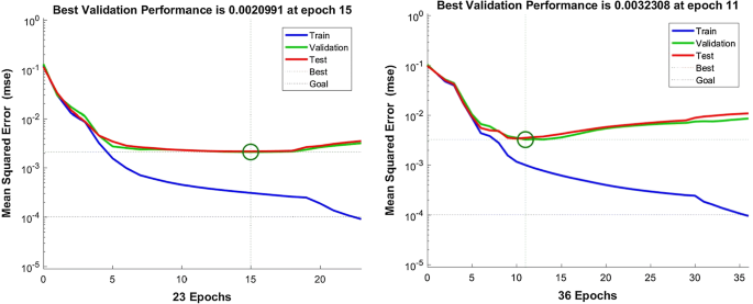
Optimal epoch selection for the ANN model training considered in this study
- (b)
The model performance converges to the goal (set at 0.0001).
- (c)
The performance gradient falls below the set minimum gradient (set at 10−7).
- (d)
The ‘Mu’ value exceeds the maximum set value (Set at 1010).
- (e)
Validation performance has increased more than the maximum set failure time since the last time it decreased (Set at 20).

The performance of the ANN model is evaluated through the use of three criterions: Eqs. (20)–(22) describes the mathematical expression of the coefficient of correlation (R), mean squared error (MSE), and mean absolute error (MAE), respectively, for the predicted estimates values against their counterpart real values.
where \(N\) = total number of samples, \(X_{i}\) = actual values, \(Y_{i}\) = predicted values, \(\bar{X}_{i}\) = \(\sum\nolimits_{i = 1}^{N} {\frac{{\left( {X_{i} } \right)}}{N}}\) and \(S_{x}\) = \(\sqrt {\frac{{\left( {X_{i} - \bar{X}_{i} } \right)^{2} }}{N - 1}}\), same for the \(\bar{Y}_{i}\) and \(S_{y}\).
4 Results and discussion
4.1 Optimum ANN model and predictions
Table 4a, b describes the different learning algorithms available to train the ANN model for hourly and daily, all of which were considered in this study to identify the best algorithm after experimenting with the available dataset. It can be seen that the Levenberg–Marquardt (LM) training algorithm is the standout performer when it comes to ANN model prediction accuracies (lowest MSE, MAE).
After the best training algorithm was determined, ANN models were trained as a part of a comparative study in which a different combinations of hidden layers and hidden neurons in each layer was tried and tested for the four target-data case scenarios discussed in Sect. 3.2.4. Six different ANN architectures were considered for each case, and hence, a total of 24 neural network models were trained for each—daily and hourly analyses. All the ANN models showed high correlation between the chosen inputs and targets, in terms of R value varying between 0.96 and 0.98. The trained models were then used to make predictions for the PDb, which was removed from the ANN training dataset. Figure 8 represents the ANN performance results for all the 24 ANN models, in terms of the prediction accuracies (MSE, MAE, and R) as discussed in Sect. 3.2.4, along with the ANN model training time.

ANN performance for six architectures designed for each of the four energy target-data cases: a daily analysis, b hourly analysis
From Fig. 8 (daily cases), it can be seen that for Case 1, the TL-2N ANN model is marginally better than the other five architectures in terms of the combination of prediction accuracies and model training time. Similarly, SL-2N, TL-2N, and TL-3N are observably the optimum ANN architectures for Cases 2, 3, and 4, respectively. Figure 9 (daily cases) describes the performance of each of these four optimal ANN models in terms of the correlation of individual model-predicted target values with the actual recorded target values pertaining to the PDb. The electricity (Elec.) and gas graphs are further divided into two scales to accommodate the different data scales estimated by the four target-data case studies. Based on these two figures, it can be seen that of all the ANN models, TL-2N model for Case 3 is the best ANN model for daily scale analysis with the smallest error in prediction values (MSE = 0.1%, MAE = 2%), with the model trained and tested in MATLAB in only 8 s.

ANN prediction accuracies for each of the four identified targets representing indoor microclimatic conditions—T and RH, and NGS energy consumption—gas and electricity
The same procedure was followed for the hourly analysis. From Fig. 8 (hourly cases), it can be observed that hourly cases also experienced uniformly high correlation (R between 0.97 and 0.99) between the ANN model predictions and the PDb targets. It is, however, clearly visible that the ANN models belonging to Cases 3 and 4 performed the poorest. TL-3N and DL-3N are the two ANN architectures with the best performances in these two cases. The optimal ANN architectures for Cases 1 and 2 were identified to be TL-3N and DL-3N, respectively. Figure 9 (hourly cases) highlights the performance of the four optimal ANN models from the four cases based on correlation of each individual model-predicted output with their PDb counterpart from the same time period. The electricity and gas graphs are further divided into two, as done in the daily analysis. From the two figures, DL-3N of Case 2 is identified as the optimal hourly scale ANN model. This indicates that if the analysis is zoomed into hourly scale, then the owing to the complex nature of this scale of analysis, the ANN model, performs better with the NGS energy consumption scaled down to the possible energy requirements from Gallery-11 with the help of assumptions as discussed in Sect. 3.2.2.
4.2 System identification (SID) of the NGS building environment
The best ANN architecture from the most adequate data processing case study was selected as the optimal ANN-based SID model which identified the complex NGS building system in terms of the optimal indoor microclimatic conditions for artwork conservation (indoor air T, RH) and the NGS building energy consumption (gas, electricity). This step was performed on a daily scale and a more detailed hourly scale involving the building opening hours and occupancy patterns, using separate ANN models as discussed in the previous section. The SID obtained from the optimal ANN model was validated by checking the correlation of the ANN model-generated target values with the actual recorded values of the same (real data from the BMS, corresponding to the same time period as the ANN predictions), which were not involved in the ANN training and testing cases (PDb). Figure 10 highlights this validation. Figure 10 (top) shows the comparison of the ANN-based SID estimates of indoor T, RH, and NGS gas and electricity consumption with the recorded real data from the same time period consumption on a daily scale. Figure 10 (bottom) highlights the same in a more detailed hourly case. To check the accuracy of the hourly prediction ANN model in detail, three further sections of Fig. 10 (bottom) for three different ranges of samples, i.e. 340–440 (as described in Fig. 11), 940–1060 (as described in Fig. 12), and 1540–1660 (as in described Fig. 13).

ANN-based SSID of the NGS building for a daily analyses, b hourly analyses

ANN-based SSID of the NGS building for hourly analyses for samples 340–460

ANN-based SSID of the NGS building for hourly analyses for samples 940–1060

ANN-based SSID of the NGS building for hourly analyses for samples 1540–1660
5 Conclusion
In this study, ANN has been utilised to predict the indoor microclimatic parameters critical for artwork conservation along with the building energy use in a historical art gallery building of great cultural significance. A set of four rough approximation-based case studies were designed and implemented to process the target data for improving the ANN performance. The ANN model development program in the study considered an experiment of six different combinations of hidden layers and number of hidden neurons, separately on two temporal scales—daily and hourly, for each case study. Different training algorithms were also considered in the experiment from which the Levenberg–Marquardt (LM) algorithm proved to be the best based on prediction accuracies.
The results of the developed ANN models were evaluated on statistical platform of error and performance metrics in comparison with a randomly separated fraction of the historical records excluded from the ANN training dataset. From the error analysis, the robust predicting ability of ANN models was demonstrated with the prediction data matching the actual data in terms of high overall accuracy with correlation coefficient (R) values ranging from 0.96 to 0.99. The MSE and MAE were observed to be within acceptable ranges of 0.1–0.3% and 2–4%, respectively, for daily scale analyses and of 0.05–0.18% and 1.8–2.7%, respectively, for hourly scale analyses. The two ANN-based system identification (SID) models for daily and hourly scales were TL-2N from target-data Case-3 and DL-3N from Case-2, respectively, based on maximum performance of the models in their respective analysis data scales.
It is thus concluded that ANNs are able to work with limited amount of building system data (real data) readily available from the building management. Using this, it can emulate an otherwise complex and strongly coupled building system in terms of different zones, operating hours, occupancy, energy consumption, and optimal indoor environment for collections’ care. Hence, the ANN model could be tailored into a module and built into a BMS system to improve forecasting and collecting data for evidence-based decision making to achieve real and effective optimisation for system operation. The study further reinstates that the ANN-based SI model can prove to be an ideal platform to investigate various optimisation strategies of the building operation in future, especially in the case of restrictive traditional building types where any retrofit solution needs a strong scientific backing of guaranteed success before practical implementation.
Abbreviations
- AHU:
-
Air handling unit
- ANN:
-
Artificial neural network
- BMS:
-
Building management system
- C1–C4:
-
Case 1–Case 4
- CAV:
-
Constant air volume system
- DC:
-
Daily case
- HC:
-
Hourly case
- HVAC:
-
Heating ventilation and air conditioning
- HWD:
-
Hourly weights distribution
- MAE:
-
Mean absolute error
- MSE:
-
Mean square error
- NGS:
-
National galleries of Scotland
- SID:
-
System identification
- TDb:
-
Training database
- PDb:
-
Prediction database
- \(A\) :
-
Area (m2)
- \(C_{p}\) :
-
Specific heat (kJ/kg K)
- \(E\) :
-
Electricity consumption (kW)
- \(g\) :
-
Moisture content (kg/kg dry air)
- \(G\) :
-
Gas consumption (kWh)
- \(Hi\) :
-
ANN hidden layer
- \(In\) :
-
ANN input layer
- \(i, j, k\) :
-
Hidden layer notations
- \(\dot{m}\) :
-
Mass flow rate (kg/s)
- \(n\) :
-
Outdoor air damper (%)
- \(n_{\text{HVAC}}\) :
-
HVAC’s contribution in energy consumption
- \(N_{\text{m}}\) :
-
Number of days in month
- \(N_{\text{occ}}\) :
-
Number of occupants
- \(R\) :
-
Coefficient of correlation
- \({\text{RH}}\) :
-
Relative humidity (%)
- \(T\) :
-
Temperature (°C)
- \({\text{Ta}}\) :
-
ANN target layer
- \(\dot{v}\) :
-
Volumetric air flow rate (m3/s)
- \(V\) :
-
Volume (m3)
- \(W\) :
-
ANN synapse weight
- \(x\) :
-
ANN neuron input
- \(X\) :
-
Input variable
- \(y\) :
-
ANN neuron output
- \(\Delta h_{\text{vap}}\) :
-
Latent heat of vaporisation (kJ/kg)
- \(\varphi\) :
-
Sensible heat (kW)
- b:
-
Bias
- D:
-
Daily
- h:
-
Hourly
- hh:
-
Half-hourly
- m:
-
Mixed
- M:
-
Monthly
- nth:
-
Non-thursday weekday
- o:
-
Outdoor
- occ:
-
Occupants
- R:
-
Room
- ret:
-
Return
- s:
-
Supply
- th:
-
Thursday
References
Fazeli R, Davidsdottir B, Hallgrimsson JH (2016) Residential energy demand for space heating in the Nordic countries: accounting for interfuel substitution. Renew Sustain Energy Rev 57:1210–1226. https://doi.org/10.1016/j.rser.2015.12.184
Constantinescu T (2011) Europe’s buildings under the microscope: a country-by-country review of the energy performance of buildings. Building Performance Institute Europe (BPIE), Brussels
Ciulla G, Lo Brano V, D’Amico A (2016) Modelling relationship among energy demand, climate and office building features: a cluster analysis at European level. Appl Energy 183:1021. https://doi.org/10.1016/j.apenergy.2016.09.046
Corgnati SP, Filippi M (2010) Assessment of thermo-hygrometric quality in museums: method and in-field application to the “Duccio di Buoninsegna” exhibition at Santa Maria della Scala (Siena, Italy). J Cult Herit 11:345–349
Corgnati SP, Fabi V, Filippi M (2009) A methodology for microclimatic quality evaluation in museums: application to a temporary exhibit. Build Environ 44:1253–1260
Kramer RP, Maas MPE, Martens MHJ, van Schijndel AWM, Schellen HL (2015) Energy conservation in museums using different setpoint strategies: a case study for a state-of-the-art museum using building simulations. Appl Energy 158:446–458
Ascione F, Bellia L, Capozzoli A, Minichiello F (2009) Energy saving strategies in air-conditioning for museums. Appl Therm Eng 29:676–686. https://doi.org/10.1016/j.applthermaleng.2008.03.040
Wang F, Pichetwattana K, Hendry R, Galbraith R (2014) Thermal performance of a gallery and refurbishment solutions. Energy Build 71:38–52
Bellia L, Capozzoli A, Mazzei P, Minichiello F (2007) A comparison of HVAC systems for artwork conservation. Int J Refrig 30:1439–1451. https://doi.org/10.1016/j.ijrefrig.2007.03.005
Huang H, Chen L, Mohammadzaheri M, Hu E, Chen M (2013) Multi-zone temperature prediction in a commercial building using artificial neural network model. In: 2013 10th IEEE international conference on control automation, pp 1896–1901. https://doi.org/10.1109/icca.2013.6565010
Little J, Ferraro C, Aregi B (2015) Assessing risks in insulation retrofits using hygrothermal software tools: heat and moisture transport in internally insulated stone walls. Historic Scotland Technical Paper 15. https://doi.org/10.13140/rg.2.1.2493.3844
Ferdyn-Grygierek J (2014) Indoor environment quality in the museum building and its effect on heating and cooling demand. Energy Build 85:32–44
Kohler M, Blond N, Clappier A (2016) A city scale degree-day method to assess building space heating energy demands in Strasbourg Eurometropolis (France). Appl Energy 184:40–54. https://doi.org/10.1016/j.apenergy.2016.09.075
Shaikh PH, Nor NBM, Nallagownden P, Elamvazuthi I, Ibrahim T (2014) A review on optimized control systems for building energy and comfort management of smart sustainable buildings. Renew Sustain Energy Rev 34:409–429. https://doi.org/10.1016/j.rser.2014.03.027
Li X, Wen J (2014) Review of building energy modeling for control and operation. Renew Sustain Energy Rev 37:517–537. https://doi.org/10.1016/j.rser.2014.05.056
Carbon Trust (2011) Closing the gap: lessons learned on realising the potential of low carbon building design. Carbon Trust
National Measurement Network (2012) The building performance gap—closing it through better measurement Event report Wednesday 5 December 2012 ARUP, 13 Fitzroy Street, London, W1T 4BQ Measurement Network. www.npl.co.uk/measurement-network
Kramer RP, van Schijndel AWM, Schellen HL (2016) The importance of integrally simulating the building, HVAC and control systems, and occupants’ impact for energy predictions of buildings including temperature and humidity control: validated case study museum Hermitage Amsterdam. J Build Perform Simul 1493:1–22. https://doi.org/10.1080/19401493.2016.1221996
Oldewurtel F, Parisio A, Jones CN, Gyalistras D, Gwerder M, Stauch V, Lehmann B, Morari M (2012) Use of model predictive control and weather forecasts for energy efficient building climate control. Energy Build 45:15–27. https://doi.org/10.1016/j.enbuild.2011.09.022
Platt G, Li J, Li R, Poulton G, James G, Wall J (2010) Adaptive HVAC zone modeling for sustainable buildings. Energy Build 42:412–421. https://doi.org/10.1016/j.enbuild.2009.10.009
Crawley DB, Hand JW, Kummert M, Griffith BT (2008) Contrasting the capabilities of building energy performance simulation programs. Build Environ 43:661–673
Braun JE (1990) Reducing energy costs and peak electrical demand through optimal control of building thermal storage. ASHRAE Trans 96:876–888. https://doi.org/10.1017/CBO9781107415324.004
Lee KH, Braun JE (2008) Model-based demand-limiting control of building thermal mass. Build Environ 43:1633–1646. https://doi.org/10.1016/j.buildenv.2007.10.009
Nassif N, Moujaes S, Zaheeruddin M (2008) Self-tuning dynamic models of HVAC system components. Energy Build 40:1709–1720. https://doi.org/10.1016/j.enbuild.2008.02.026
Nassif N (2013) Modeling and optimization of HVAC systems using artificial neural network and genetic algorithm. Build Simul 7:237–245. https://doi.org/10.1007/s12273-013-0138-3
Tashtoush B, Molhim M, Al-Rousan M (2005) Dynamic model of an HVAC system for control analysis. Energy 30:1729–1745. https://doi.org/10.1016/j.energy.2004.10.004
Kiran MS, Özceylan E, Gündüz M, Paksoy T (2012) Swarm intelligence approaches to estimate electricity energy demand in Turkey. Knowl Based Syst 36:93–103. https://doi.org/10.1016/j.knosys.2012.06.009
Lee YS, Tong LI (2011) Forecasting time series using a methodology based on autoregressive integrated moving average and genetic programming. Knowl Based Syst 24:66–72. https://doi.org/10.1016/j.knosys.2010.07.006
Ltifi H, Benmohamed E, Kolski C, Ben Ayed M (2016) Enhanced visual data mining process for dynamic decision-making. Knowl Based Syst 112:166–181. https://doi.org/10.1016/j.knosys.2016.09.009
Ma J, Qin J, Salsbury T, Xu P (2012) Demand reduction in building energy systems based on economic model predictive control. Chem Eng Sci 67:92–100. https://doi.org/10.1016/j.ces.2011.07.052
Xu J, Wang Y, Tao Z (2013) Rough approximation based strategy model between a green building developer and a contractor under a fuzzy environment. Knowl Based Syst 46:54–68. https://doi.org/10.1016/j.knosys.2013.03.002
Nilashi M, Zakaria R, Ibrahim O, Majid MZA, Mohamad Zin R, Chugtai MW, Zainal Abidin NI, Sahamir SR, Aminu Yakubu D (2015) A knowledge-based expert system for assessing the performance level of green buildings. Knowl Based Syst 86:194–209. https://doi.org/10.1016/j.knosys.2015.06.009
Yun K, Luck R, Mago PJ, Cho H (2012) Building hourly thermal load prediction using an indexed ARX model. Energy Build 54:225–233. https://doi.org/10.1016/j.enbuild.2012.08.007
Eisenhower B, O’Neill Z, Narayanan S, Fonoberov VA, Mezić I (2012) A methodology for meta-model based optimization in building energy models. Energy Build 47:292–301. https://doi.org/10.1016/j.enbuild.2011.12.001
Shin M, Do SL (2016) Prediction of cooling energy use in buildings using an enthalpy-based cooling degree days method in a hot and humid climate. Energy Build. https://doi.org/10.1016/j.enbuild.2015.10.035
Zhu J, Yang Q, Lu J, Zheng B, Yan C (2015) An adaptive artificial neural network-based supply air temperature controller for air handling unit. Trans Inst Meas Control 37:1118–1126. https://doi.org/10.1177/0142331214557171
Yuce B, Li H, Rezgui Y, Petri I, Jayan B, Yang C (2014) Utilizing artificial neural network to predict energy consumption and thermal comfort level: an indoor swimming pool case study. Energy Build 80:45–56. https://doi.org/10.1016/j.enbuild.2014.04.052
Sanjari MJ, Karami H, Gooi HB (2016) Micro-generation dispatch in a smart residential multi-carrier energy system considering demand forecast error. Energy Convers Manag 120:90–99. https://doi.org/10.1016/j.enconman.2016.04.092
Kwok SSK (2011) A study of the importance of occupancy to building cooling load in prediction by intelligent approach. Energy Convers Manag 52:2555–2564. https://doi.org/10.1016/j.enconman.2011.02.002
Ben-Nakhi AE, Mahmoud MA (2004) Cooling load prediction for buildings using general regression neural networks. Energy Convers Manag 45:2127–2141. https://doi.org/10.1016/j.enconman.2003.10.009
Li Q, Meng Q, Cai J, Yoshino H, Mochida A (2009) Predicting hourly cooling load in the building: a comparison of support vector machine and different artificial neural networks. Energy Convers Manag 50:90–96. https://doi.org/10.1016/j.enconman.2008.08.033
Chandok JS, Kar IN, Tuli S (2008) Estimation of furnace exit gas temperature (FEGT) using optimized radial basis and back-propagation neural networks. Energy Convers Manag 49:1989–1998. https://doi.org/10.1016/j.enconman.2008.03.011
Mohanty S (2009) Artificial neural network based system identification and model predictive control of a flotation column. J Process Control 19:991–999. https://doi.org/10.1016/j.jprocont.2009.01.001
Asgari H, Chen X, Menhaj MB, Sainudiin R (2013) Artificial neural network-based system identification for a single-shaft gas turbine. J Eng Gas Turbines Power 135:92601. https://doi.org/10.1115/1.4024735
Roy S, Banerjee R, Das AK, Bose PK (2014) Development of an ANN based system identification tool to estimate the performance-emission characteristics of a CRDI assisted CNG dual fuel diesel engine. J Nat Gas Sci Eng 21:147–158. https://doi.org/10.1016/j.jngse.2014.08.002
Li X, Wen J, Bai EW (2016) Developing a whole building cooling energy forecasting model for on-line operation optimization using proactive system identification. Appl Energy 164:69–88. https://doi.org/10.1016/j.apenergy.2015.12.002
Nandagopal MSG, Abraham E, Selvaraju N (2017) Advanced neural network prediction and system identification of liquid–liquid flow patterns in circular microchannels with varying angle of confluence. Chem Eng J 309:850–865. https://doi.org/10.1016/j.cej.2016.10.106
Akramin MRM, Ariffin AK, Kikuchi M, Abdullah S (2017) Sampling method in probabilistic S-version finite element analysis for initial flaw size. J Braz Soc Mech Sci Eng 39:357–365. https://doi.org/10.1007/s40430-016-0549-z
Acknowledgements
The authors thank Michael Browne and Charles Sclater from the NGS for providing the vital access to historical data pertaining to the building. The study is part of a funded Ph.D. program facilitated by collaboration of the National Galleries of Scotland (NGS), Energy Technology Partnership (ETP)—Scotland, and the Heriot-Watt University.
Author information
Authors and Affiliations
Corresponding author
Additional information
Publisher's Note
Springer Nature remains neutral with regard to jurisdictional claims in published maps and institutional affiliations.
Rights and permissions
Open Access This article is distributed under the terms of the Creative Commons Attribution 4.0 International License (http://creativecommons.org/licenses/by/4.0/), which permits unrestricted use, distribution, and reproduction in any medium, provided you give appropriate credit to the original author(s) and the source, provide a link to the Creative Commons license, and indicate if changes were made.
About this article

Cite this article
Ganguly, S., Ahmed, A. & Wang, F. Optimised building energy and indoor microclimatic predictions using knowledge-based system identification in a historical art gallery. Neural Comput & Applic 32, 3349–3366 (2020). https://doi.org/10.1007/s00521-019-04224-7
Received:
Accepted:
Published:
Issue Date:
DOI: https://doi.org/10.1007/s00521-019-04224-7