
Abstract
Flood mitigation should deal with those most sensitive flooding elements to very efficiently release risks and reduce losses. Present the most concerns of flood control are peak level or peak discharge which, however, may not always be the most sensitive flooding element. Actually, along with human activities and climate change, floods bring threats to bear on human beings appear in not only peak level and peak discharge, but also other elements like maximum 24-h volume and maximum 72-h volume. In this paper, by collecting six key flooding intensity indices (elements), a catastrophe progression approach based sensitivity analysis algorithm model is developed to identify the indices that mostly control over the flood intensity. The indices sensitivity is determined through a selected case study in the Wujiang River, South China, based on half a century of flow record. The model results indicate that there is no evident relationship of interplay among the index sensitivities, but the variability of the index sensitivity is closely related to the index variability and the index sensitivity increases with the decrease of index value. It is found that peak discharge is not the most influential flooding factor as is generally thought in this case. The sensitivity value of the maximum 24-h volume is the greatest influential factor among all the other indices, indicating that this index plays a leading role in the flood threat of the Wujiang River, South China. It is inferred that, for the purpose of flood warning and mitigation, the peak flood discharge is not always the most sensitive and dominant index as opposed to the others, depending on the sensitivity.
1 Introduction
Extreme hydrological events are inevitable and stochastic in nature (Shiau 2003). To mitigate the loss and suffering brought by flooding, various methodologies, such as flood forecasting and simulation and disaster evaluation (Zhao et al. 2007), have been applied to inform precautionary measures with a focus on sensitive flooding elements. Flood process is characterized by multi-elements, e.g., peak level, peak discharge and volume, and shows the influence by flood intensity (Wang et al. 2015). Generally, flood peak values are required in the design of bridges, culverts, waterways, dam spillways and the estimation of scour at hydraulic structures (Khant et al. 2014). Lehner et al. (2006) pointed out the analysis of peak flood discharges is required to correlate the magnitude and frequency of high runoffs with that of probability of future occurrence. This probability is derived from statistical analyses of yearly level/discharge maxima or levels/discharges above a threshold (Schumann 2011). So, many literatures (Adamowski 2000; Fernandes et al. 2010; Villarini and Smith 2010; Ahmad et al. 2012) show that the peak discharge is one of the most important index on flood intensity, which reflect the flood magnitude. Meanwhile, there are a lot of papers devoted to study the influence of other indices on the flood intensity. For example, water depth is a widely used index for flood damage assessment (NRC 2000; Merz et al. 2004; Jonkman 2010), and is also regarded as a key measure of flood magnitude. Ahmed and Mirza (2000) pointed out that the flood intensity index should be calculated from the flood duration (number of days). Halmova et al. (2008) express the opinion that the maximum annual t-day flood volume should be considered. But unfortunately these literatures have not been performed to quantify the effect of all these indices together on flood intensity. Quantifying the effect of various indices on flood intensity is a difficult task due to the unknown and the high nonlinearities in the impact of these indices and flood intensity.
As previous studies deal mostly with uncertainty related to flood intensity (Solana-Ortega and Solana 2001; Apel et al. 2004; Downton et al. 2005; Merz et al. 2004; Apel et al. 2008; Chen et al. 2013), a need exists for a methodology to evaluate the sensitivity of indices associated with the flood intensity. Sensitivity analysis is a branch of numerical analysis that aims to quantify the impact of index variability on the output of a numerical model (McCarthy et al. 2001; Wagener et al. 2001; Hall et al. 2005; Perry et al. 2008; Saltelli et al. 2008; Rosolem et al. 2012; Pianosi et al. 2014; Pianosi and Wagener 2015). There are numerous studies in literature devoted to sensitivity analysis for solving economics problems such as investment projects and spatial Welfare (Agro et al. 1997; Dick et al. 1994; Kratena et al. 2012; Sacristán et al. 1995). Sensitivity analysis of the flood intensity indices, however, is poorly reported in the literature. The analysis of the indices influencing the flood intensity is always a research hotspot in hydrology. Indices such as peak discharge, peak stage and flood duration have the most restrictive effect on the flooding process. In this paper, the catastrophe progression based sensitivity analysis algorithm (SAA) method, as a very strong approach for effectively assessing the relationship between indices and intensity of floods, is adopted to detect the indices that have most control over the flood intensity for flood risk and disaster mitigation.
So far, there has been no unity and common index that can be used to reflect flood intensity with only flood peak discharge/level being concerned. The description of flood intensity, however, should include multiple indices involved in a flood process. There are probably several reasons for choosing suitable indices reflecting the flood intensity. (1) Peak discharge, total flood volume and flood hydrograph are three most classic elements reflecting flood process, so peak discharge and total flood volume are firstly chosen. (2) To some extent, flood hydrograph being used to reflect flood intensity is very abstract, so some quantized feature values which can reflect the flood hydrograph are chosen, such as flood duration and period flood volumes. (3) Base on the past achievement (Balocki and Burges 1994; Bradley and Potter 1992; Yan and Edwards 2013; Zeng et al. 2014), maximum 24-h volume and maximum 72-h volume are the most suitable period flood volumes, which are commonly used for reflecting the flood intensity. So maximum 24-h volume and maximum 72-h volume are chosen. (4) Peak stage, which not only shows the flood hydrograph but also can reflect the flood intensity, is one of the most concerning data for the flood control department, so it is also chosen. The main objective of this study is to provide better understanding of flood intensity behavior by index sensitivity analysis. The key flood intensity indices examined in this case study and which underpin the sensitivity analysis model are the following:
-
peak discharge, the maximum discharge in cubic meters per second of a flood event;
-
peak stage, the water level in meters corresponding to the peak discharge;
-
maximum 24-h volume, the maximum water volume cubic meters for a 24-h period of a flood event;
-
maximum 72-h volume, the maximum water volume in cubic meters for a 72-h period of a flood event,
-
total flood volume, the total volume in cubic meters associated with a flood event; and
-
flood duration, the time period in hours between the start and end of a flood event.
This case study explores the sensitivity of indices that describe the flood intensity of the Wujiang River, South China. According to JRC (2011), sensitivity analysis studies how the variation in the output of a model can be apportioned, qualitatively or quantitatively, to different sources of variation. Similarly, Saltelli et al. (2000) indicated that sensitivity analysis explores the information relationship between model inputs and outputs and identifies the sources of variation influencing model outputs. It is proposed that the degree of sensitivity (influence) of an index can be quantitatively described by a sensitivity value represented by the quotient of largest output (numerator) and smallest input (denominator), when changing (perturbing) one index at a time (Srikanta 2009). The sensitivity of an index to the flood intensity is defined as its degree of impact on the flood intensity; the more sensitive an index is, the greater variation it causes in the flood intensity. The sensitivity analysis method can be given in various forms, the most common of which is that of partial derivatives (Ciftcioglu 2003) as adopted in this study and expressed by the equations.
or
where y is the output and x the input vector receptivity.
The work of this paper is (1) to build the SAA model to describe the relationship between the input variables (peak discharge, peak stage, flood duration, etc.) and the output variables (response of the flood intensity) based on real flooding events, and (2) to reveal the key influential factors and the index sensitivity features for flood intensity, which helps hydrologists to identify the dominant (most sensitive) flooding indices for flood warning and flood control.
2 Study area and data
The Wujiang River Basin, covering an area of 7097 km2 with a reach length of 260 km, is located in south of the Wuling Mountains between latitude 24°46′–25°41′N and longitude 112°23′–113°36′E as shown in Fig. 1. This area enjoys a typical subtropical climate with a mean annual rainfall of 1450 mm. The summer climate is dominated by the southwest and southeast Asian monsoons resulting in a comparatively high humidity and uneven distribution of precipitation through the season. The median discharge for the period of record is 2350 m3/s in 1992, with maximum and minimum recorded discharges of 8800 m3/s in 2006 and 630 m3/s in 1963 respectively.

Location of the study area and hydrological gauging station
Lishi gauging station (Fig. 1), located near the mouth of the Wujiang River, serves a drainage area of nearly 6976 km2, which accounts for 98 % of the Wujiang River Basin. Annual flood data records compiled by Shaoguan Branch of Guangdong Provincial Bureau of Hydrology span 53 years from 1955 to 2007, which covers the ordinary year 1992, wet year 2006 and drought year 1963. One flood process was selected from each year to form the sample series (totally 53 flood events). Only one flood event corresponding to the maximum peak flow in a year should be chosen as a study sample no matter how many flood events happened in the year. For example, there were four floods in 1999, the fourth flood series has the biggest peak flood (2850 m3/s), which is much bigger than that of the first (933 m3/s), the second (2230 m3/s) and the third (1740 m3/s) flood series. Therefore the fourth flood series has been chosen in 1999. This keeps the representativeness of flood event samples to cover the data in ordinary, wet and drought years. Moreover, the six indices (flood duration, peak discharge, the maximum 24-h flood volume, the maximum 72-h flood volume and flood volume) describing the flood intensity in this paper can fully capture the critical features of flood processes.
3 Methodology
3.1 Determination of flood duration
For each year, the biggest peak flood is picked out from all the floods for analysis in this paper. Taking a flood event in 1999 as an example, one can depict the flood process as shown in Fig. 2. It can be seen that the flood event is characterized by its peak and duration. Although there were four floods in 1999 only that one with the biggest peak can be chosen to be the sample. Flood IV has the biggest peak flood (2850 m3/s), which is bigger than that of flood I, II and III (Fig. 2). Then, the beginning (or end) time of this flood is the nearest bottom point on the left (or right) of the peak flow, as shown in Fig. 2. The duration of this flood event is measured as the time difference between point A and B. Therefore, the flood duration of this event is 150 h, which is the time span from September 16th, 14:00 (point A) to September 22th, 20:00 (point B) in Fig. 2.

Illustration of the determination of flood duration using the flood processes in year 1999
3.2 Calculations of V 24 , V 72 and V
We take the calculation of the maximum 24-h flood volume as an example. For a hypothetical flow process given in Fig. 3, the 24-h flood volume (\((V^{\prime}_{24} )_{{T_{s} }}\)) is determined by the following equation:

A hypothetical flood to demonstrate the calculation of the maximum 24-h volume
where Q k is the observed discharge of the kth hour for a flood event, \(T_{s} = 1,2, \ldots ,t - 23\) and t is no more than the flood duration. T e − T s equals 24 h. The maximum 24-h flood volume (V 24) is then defined by \(V_{24} = \hbox{max} \{ (V^{\prime}_{24} )_{{T_{s} }} \}\).
The calculation of V 72, the maximum 72-h flood volume, is similar to that of V 24.
According to the definition the total flood volume (V) is determined by
where V is the total flood volume, Q k is the observed discharge of the kth hour for a flood event, t 1 is the beginning time, t 2 is the end time.
3.3 SAA algorithm
One index can be defined as sensitive index if only minor changes to it have a large influence on the simulation results (Sieber and Uhlenbrook 2005). Insensitive indices are defined conversely. Index sensitivity analysis is used to determine how “sensitive” an index is for a given model. The index values were restricted to the recorded flood processes. Identifying the beginning and ending of a flood process are worked out in detail in the past work (Wang et al. 2015). The influence of each index on the flood intensity simulations was studied in turn to find the sensitivity of each index by varying its value while keeping the others unchanged. A flow diagram of this approach is shown in Fig. 4, and each step is described as follows.

Flowchart of the SAA model
-
Step 1 select the flooding process \(GC_{i}^{0}\):
As there are 53 flood events in the Wujiang River discharge record, the sensitivity analysis starts with \(GC_{i}^{0}\)(i = 1) where \(i \in [1,n]\) and n = 53.
-
Step 2 initialize the matrix \(mt^{0}\):
Each flooding process is defined by the six indices, flood peak, peak stage, maximum 24-h volume, maximum 72-h volume, total flood volume and flood duration such that \(GC_{i}^{0} = \{ prm_{i1}^{0} ,prm_{i2}^{0} , \ldots ,prm_{ij}^{0} , \ldots ,prm_{ip}^{0} \}\) where i ∊ [1, n] (n as in Step 1 and j ∊ [1, p] with p = 6. The matrix mt 0 is then formulated as follows:
$$mt^{0} = \left[ {\begin{array}{*{20}c} {\begin{array}{*{20}c} {prm_{i1}^{0} } \\ {prm_{i1}^{0} } \\ \ldots \\ {prm_{i1}^{0} } \\ \end{array} } & {\begin{array}{*{20}c} {prm_{i2}^{0} } \\ {prm_{i1}^{0} } \\ \ldots \\ {prm_{i2}^{0} } \\ \end{array} } & {\begin{array}{*{20}c} { \ldots ,prm_{ij}^{0} , \ldots } \\ { \ldots ,prm_{ij}^{0} , \ldots } \\ \ldots \\ { \ldots ,prm_{ij}^{0} , \ldots } \\ \end{array} } & {\begin{array}{*{20}c} {prm_{ip}^{0} } \\ {prm_{ip}^{0} } \\ \ldots \\ {prm_{ip}^{0} } \\ \end{array} } \\ \end{array} } \right],$$(5)where \(prm_{ij}^{0}\) is the jth index of the ith flooding process to yield n = 53 rows and p = 6 columns. For example, the term \(prm_{i1}^{0}\) is the flood peak of the ith flood process, \(prm_{i2}^{0}\) the peak stage, \(prm_{i3}^{0}\) the maximum 24-h volume, \(prm_{i4}^{0}\) the maximum 72-h volume, \(prm_{i5}^{0}\) the total flood volume, and \(prm_{i6}^{0}\) the flood duration.
-
Step 3 determine the index (SP 0 j ):
The influence that index changes have on the output can be determined according to the term
$$SP_{j}^{0} = \left\{ {sort\left[ {\left( {prm_{1j}^{0} ,prm_{2j}^{0} , \ldots ,prm_{ij}^{0} , \ldots ,prm_{nj}^{0} } \right),A} \right]} \right\}'$$(6)where \(prm_{ij}^{0}\) can be seen in Step 2, with A denoting an ascending sort order.
The rank corresponding to the sort order is obtained from
$$SP_{j} = (sp_{1j} ,sp_{2j} , \ldots ,sp_{nj} )^{\prime}$$(7)where n as in Step 1.
-
Step 4 form the reference matrix(mt):
Using the mt 0 from Eq. 5 and SP j from Eq. 7, solving for mt gives
$$mt = \left[ {\begin{array}{*{20}c} {prm_{{i1}}^{0} } & {prm_{{i2}}^{0} } & \ldots & {sp_{{1j}} } & \ldots & {prm_{{ip}}^{0} } \\ {prm_{{i1}}^{0} } & {prm_{{i2}}^{0} } & \ldots & {sp_{{2j}} } & \ldots & {prm_{{ip}}^{0} } \\ \ldots & \ldots & \ldots & \ldots & \ldots & \ldots \\ {prm_{{i1}}^{0} } & {prm_{{i2}}^{0} } & \ldots & {sp_{{nj}} } & \ldots & {prm_{{ip}}^{0} } \\ \end{array} } \right]$$(8)where \(i \in [1,n]\) as in Step 1, \(j \in [1,p]\) as in Step 2. The reference matrix (mt) has 53 rows and 6 columns.
-
Step 5 find tracing position (l)
According to the reference matrix (mt) and the selected flooding process (GC 0 i ), the element in matrix (mt) which is equal to \(GC_{i}^{0}\) \(( i \in [1,n] )\) in value is denoted to be the lth element.
For the rank (SP j ) in Step 3, sp lj is corresponding to the jth index in GC 0 i .
-
Step 6 calculate the evaluation value of the flood intensity vector (FIM):
This paper investigates the sensitivity of the flooding “indices” with specifying flood intensity, which is calculated by the catastrophe progression method. Catastrophe theory as originally put forward in the late 1960s by Thom (1989), lies at the heart of the index sensitivity analysis. As a multi-level factorization of target evaluation, the catastrophe progression method derives from catastrophe modeling. The model recognizes a total of seven elementary catastrophes, each of which is associated with a potential function defined by up to four control indices and one or two state variables (Zeeman 1976). The catastrophe progression approach has some advantages for easy use: it involves the relative importance of each index for evaluation with no necessity of weights for indices, which greatly reduces the subjectivity for reasonably evaluating indices, can access the relationship between indices and flood intensity, and can identify the bigger influential index to flood magnitude from various indices.
The catastrophe progression model constructed for evaluating flood intensity in the Wujiang River Basin comprises three of the seven elementary catastrophes identified by the following potential functions f(g): fold catastrophe:
$$f\left( g \right) = g^{3} + ug$$(9)cusp catastrophe:
$$f\left( g \right) = g^{4} + ug^{2} + vg$$(10)swallowtail catastrophe:
$$f\left( g \right) = g^{5} + ug^{3} + vg^{2} + wg$$(11)where g is the state variable and the coefficients u, v and w represent control indices. The application of the above concepts in the Wujiang River case study is illustrated diagrammatically in Fig. 5. The catastrophe progression method requires solving the evaluation value of the flood FIM, which is corresponding to the flood intensity value of each row in the reference matrix (mt), as follows:
$$FIM = \{ fi_{1} ,fi_{2} , \ldots ,fi_{n} \}$$(12)Fig. 5 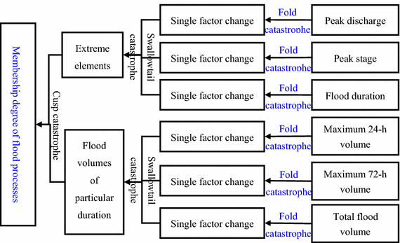
Evaluation index system for the flooding processes in the Wujiang River case study
-
Step 7 calculate the index sensitivity \(GC_{i}^{0} \_ps_{j}\):
According to the function \(\frac{\partial y}{\partial x} = \frac{y(x + \Delta x) - y(x)}{\Delta x}\) (Eq. 1) or \(\frac{\partial y}{\partial x} = \frac{y(x) - y(x - \Delta x)}{\Delta x}\) (Eq. 2), the use of this finite difference approximation requires two repeated simulation runs. In this function, the selection of an appropriate index perturbation value Δx is important.
The six indices used in this case study have different physical meaning and measurement units. In order to eliminate differences in sensitivity, data pre-treatment is needed. For the selected index (SP 0 j ), the rank result obtained from \(SP_{j} = (sp_{1j} ,sp_{2j} , \ldots ,sp_{nj} )^{\prime}\) Eq. (7) is normalized as follows:
$$\left\{ {\begin{array}{*{20}c} {n\_sp_{1j} = \frac{{sp_{1j} }}{{\hbox{max} (SP_{j} )}}} \\ {n\_sp_{2j} = \frac{{sp_{2j} }}{{\hbox{max} (SP_{j} )}}} \\ \ldots \\ {n\_sp_{nj} = \frac{{sp_{nj} }}{{\hbox{max} (SP_{j} )}}} \\ \end{array} } \right.$$(13)The measured flooding process data (flood peak, peak stage, etc.) vary from year to year, and their magnitude constitutes a hydrologic series that defines boundary conditions in the index sensitivity analysis model for the measurement location. The effect of index changes on the sensitivity analysis model output is determined by the following function:
$$GC_{i}^{0} \_PS_{j} = \left\{abs\left(\frac{{fi_{1} - fi_{2} }}{{n\_sp_{1j}- n\_sp_{2j} }}\right),\quad abs\left(\frac{{fi_{2} - fi_{3} }}{{n\_sp_{2j} - n\_sp_{3j} }}\right), \ldots ,abs\left(\frac{{fi_{(n - 1)} - fi_{n} }}{{n\_sp_{(n - 1)j} - n\_sp_{nj} }}\right)\right\}$$(14)The sensitivity of the jth index of the ith flooding process is determined as follows:
$$GC_{i}^{0} \_ps_{j} = \left\{ {\begin{array}{*{20}c} {abs\left( {\frac{{fi_{{(l + 1)}} - fi_{l} }}{{n\_sp_{{(l + 1)j}} - n\_sp_{{lj}} }}} \right),l = 1} \\ \begin{gathered} abs\left( {\frac{{fi_{l} - fi_{{(l - 1)}} }}{{n\_sp_{{lj}} - n\_sp_{{(l - 1)j}} }}} \right),l = n \hfill \\ \frac{1}{2}\left[ {abs\left( {\frac{{fi_{l} - fi_{{(l - 1)}} }}{{n\_sp_{{lj}} - n\_sp_{{(l - 1)j}} }}} \right) +\, abs\left( {\frac{{fi_{{(l + 1)}} - fi_{l} }}{{n\_sp_{{(l + 1)j}} - n\_sp_{{lj}} }}} \right)} \right],l \in (1,n) \hfill \\ \end{gathered} \\ \end{array} } \right.$$(15)where l ∊ [1, n] and j ∊ [1, p] as before. The greater the value of GC 0 i _ps j is, the more sensitive the index will be.
-
Step 8 determine the update number (j):
The initial update number for (j) is set to 1, checked to see whether it has reached the maximum update number (p), incremented by 1 if no (false) and repeating Steps 3–7, and if yes (true), terminate the simulation. All the index sensitivity values (PSV_GC 0 i ) of the selected flooding processes (GC 0 i ) are then calculated as follows:
$$PSV\_GC_{i}^{0} = \{ GC_{i}^{0} \_ps_{1} ,GC_{i}^{0} \_ps_{2} , \ldots ,GC_{i}^{0} \_ps_{p} \}$$(16) -
Step 9 determine the update number (i):
As the sensitivity of an index may differ between flooding processes (i), it is also necessary to calculate the sensitivity of each index in each flooding process. The initial update value for (i) is set to 1 and the procedure set out in Step 7 followed, with Steps 1–7 being repeated for a false result until a true one is returned. The index sensitivity values (GC 0 i _ps j ) of all the 53 flooding processes are then calculated as follows:
$$\begin{aligned} PSV = \{ PSV\_GC_{1}^{0} ,PSV\_GC_{2}^{0} , \ldots ,PSV\_GC_{n}^{0} \} \hfill \\ \begin{array}{*{20}c} {} & {} \\ \end{array} = \left[ {\begin{array}{*{20}c} {GC_{1}^{0} \_ps_{1} } & {GC_{1}^{0} \_ps_{2} } & {\begin{array}{*{20}c} \ldots & {GC_{1}^{0} \_ps_{j} } & \ldots \\ \end{array} } & {GC_{1}^{0} \_ps_{p} } \\ {GC_{2}^{0} \_ps_{1} } & {GC_{2}^{0} \_ps_{2} } & {\begin{array}{*{20}c} \ldots & {GC_{2}^{0} \_ps_{j} } & \ldots \\ \end{array} } & {GC_{2}^{0} \_ps_{p} } \\ {\begin{array}{*{20}c} \ldots \\ {GC_{i}^{0} \_ps_{1} } \\ \ldots \\ \end{array} } & {\begin{array}{*{20}c} \ldots \\ {GC_{i}^{0} \_ps_{2} } \\ \ldots \\ \end{array} } & {\begin{array}{*{20}c} {\begin{array}{*{20}c} \ldots & \ldots & \ldots \\ \end{array} } \\ {\begin{array}{*{20}c} \ldots & {GC_{i}^{0} \_ps_{j} } & \ldots \\ \end{array} } \\ {\begin{array}{*{20}c} \ldots & \ldots & \ldots \\ \end{array} } \\ \end{array} } & {\begin{array}{*{20}c} \ldots \\ {GC_{i}^{0} \_ps_{p} } \\ \ldots \\ \end{array} } \\ {GC_{n}^{0} \_ps_{1} } & {GC_{n}^{0} \_ps_{2} } & {\begin{array}{*{20}c} \ldots & {GC_{n}^{0} \_ps_{j} } & \ldots \\ \end{array} } & {GC_{n}^{0} \_ps_{p} } \\ \end{array} } \right] \hfill \\ \end{aligned}$$(17)where \(GC_{i}^{0} \_ps_{j}\) is the jth index sensitivity value of the ith flood intensity, with \(i \in [1,n]\) and \(j \in [1,p]\) as before.
-
Step 10 identify the index sensitivity for the flood intensity (S j ):
The index sensitivity of the flood intensity in the river basin is determined by the minimum index sensitivity value as follows:
$$S_{j} = \hbox{min} (GC_{1}^{0} \_ps_{j} ,GC_{2}^{0} \_ps_{j} , \ldots ,GC_{n}^{0} \_ps_{j} ) = \left\{ \begin{aligned} \hbox{min} \{ GC_{i}^{0} \_ps_{1} \} \hfill \\ \ldots \hfill \\ \hbox{min} \{ GC_{i}^{0} \_ps_{j} \} \hfill \\ \ldots \hfill \\ \hbox{min} \{ GC_{i}^{0} \_ps_{p} \} \hfill \\ \end{aligned} \right.$$(18)where \(GC_{i}^{0} \_ps_{j}\) is as for Step 8.

4 Results and discussion
4.1 Index sensitivity
The calculated sensitivity values for each of the six flooding process indices over the 53-year period of flow gauging record at Lishi Station on the Wujiang River is illustrated in Fig. 6. The graphs show the temporal variation in index sensitivity values and more specifically, the greater magnitude of the maximum 24-h and 72-h volume fluctuations compared to the other indices. It would appear that the sensitivity of indices for the Wujiang River at Lishi Station shows no significant trend over the period of record, although close visual inspection of Fig. 6f suggests a slight increase in flood duration.

Time series of index sensitivity value (ISV) at Lishi Station of the Wujiang River; a peak discharge, b peak stage, c maximum 24-h volume, d maximum 72-h volume, e total flood volume, f flood duration
Similar comparisons are presented in Fig. 7, in this instance showing the difference in inter-index sensitivity per flooding process. The most obvious feature common to all six ‘panels’ is the greater sensitivity shown by the maximum 24-h volume index compared to the other indices. This is followed in sensitivity by the maximum 72-h volume with peak stage and flood duration being the least sensitive.

Characterization of the ISV: P peak discharge; H peak stage; V24 maximum 24-h volume; V72 maximum 72-h volume; V total flood volume; T flood duration
4.2 Index value versus sensitivity
A correlation of the index value and sensitivity value for each of the 53 flood events is presented in Fig. 8. The panels (a1) to (a6) show a direct comparison. The results of a power curve \(y = \alpha x^{\beta }\) ( regression analysis for each index set are shown in Table 1.

Variations of the indices and their sensitivity values (ISV):The bold line is trend-line computed by power regression
From observation of panels (a1) to (a6) in Fig. 8, it is evident that an excellent correlation exists in each index set. The data presented in Table 1 indicates a highest correlation coefficient (R 2) value of 0.9946 associated with the maximum 72-h volume index [panel (a4)], and a lowest R 2 value of 0.9839 associated with the peak stage [panel (a2)] index. An inverse relationship (negative correlation) is evident for each index set, with the index sensitivity value decreasing with increasing index value.
Furthermore, the long-term trends in the sensitivity value (Fig. 8) are influenced by the correspondence indices. The downward trend of index sensitivity values in relation to the relativity inverse relationship with indices has affected the trend of these values. Namely, the decrease trend in indices cause increasing trend in these index sensitivity values.
4.3 Inter-index sensitivity
A scatter plot matrix of index sensitivity values is presented in Fig. 9. With six indices, the matrix comprises 6 rows and 6 columns, where the ith row and jth column of the matrix represents a scatter plot of the ith and jth index sensitivity values. The matrix of panels identified by row and column number, informs inter-index sensitivity relationships, which are given substance by the regression analysis results presented in Table 2. Inter-index sensitivity, in order of descending correlation strength, is listed as follows:

Scatter plot of the variable matrix between different ISV: S-P ISV of peak discharge; S-H ISV of flood peak stage; S-V 24 ISV of maximum 24-h flood volume; S-V 72 ISV of maximum 72-h flood volume; S-V ISV of total flood volume; S-T ISV of flood duration
-
S-P to S-V24 [panels (1, 3) and (3, 1)], a linear relationship with R 2 = 0.9547;
-
S-P to S-H [panels (1, 3) and (3, 1)], a power relationship with R 2 = 0.9356;
-
S-V24 to S-V72 [panels (1, 3) and (3, 1)], a linear relationship with R 2 = 0.9304;
-
S-H to S-V24 [panels (2, 3) and (3, 2)], a power relationship with R 2 = 0.9195;
-
S-P to S-V72 [panels (3, 4) and (4, 3)], a linear relationship with R 2 = 0.8862;
-
S-V72 to S-V [panels (4, 5) and (5, 4)], a linear relationship with R 2 = 0.8621;
-
S-H to S-V72 [panels (2, 4) and (4, 2)], a power relationship with R 2 = 0.8526;
-
S-V24 to S-V [panels (3, 5) and (5, 3)], a linear relationship with R 2 = 0.7159;
-
S-P to S-V [panels (1, 5) and (5, 1)], a power relationship with R 2 = 0.5984;
-
S-H to S-V [panels (2, 5) and (5, 2)], a power relationship with R 2 = 0.5833.
The sensitivity of the flood duration index (S-T) cannot be correlated with any of the other index sensitivities.
4.4 Index sensitivity characteristics
Index sensitivity characteristics of the Wujiang River at Lishi Station based on a statistical analysis of the data are presented in Table 3. The years 1963 and 1991 stand out as years of lowest discharge, and 2006 as the year of higher discharge in the period of record. The absolute range of index sensitivity values is defined in each instance by the difference between the maximum and minimum values.
4.5 Index sensitivity significance
An absolute measure of index sensitivity significance can only be obtained from normalized data that remove the differences caused by physical expression (discharge, volume, height and time) and associated units of measurement. This was performed in the SAA model (Eq. 13), and the results are presented in Fig. 10. The individual graphs, which are based on the respective power functions listed in Table 1, represents the best-fit regression model for each data time series. The results indicate that in the case of the Wujiang River, the maximum 24-h volume is the most sensitive index, and the flood duration is the least one.

Normalized index versus index sensitivity value with the curve of the best fit model (trend-lines computed by linear regression): Diamond peak discharge; Cross symbol peak stage; Triangle maximum 24-h volume; Plus symbol maximum 72-h volume; Minus symbol total flood volume; Circle flood duration
5 Conclusions
The application of catastrophe theory to the 53-year flow record of the Wujiang River as gauged at Lishi Station has served to rank the influence on flood intensity of six flooding process indices (peak discharge, peak stage, maximum 24-h volume, maximum 72-h volume, total flood volume and flood duration) on the basis of an analysis of their sensitivity. In this work, a sensitivity analysis algorithm model is developed to identify the most sensitive index that exerts the greatest influence.
In the case of the Wujiang River, the maximum 24-h volume is identified as the most sensitive (influential) index, followed by the maximum 72-h volume. Flood duration is identified as the least influential index. Further studies are required to determine the influence of the relationship among indices on the SAA model.
The Wujiang River is a typical mountainous river with rapid flow and large falling gradient. Records showed that five heavy floods have been occurred in 1961, 1968, 1994, 2002 and 2006 in the Wujiang River during the past three decades. And four severe floods in the Wujiang River Basin were recorded in the historical archives over a 90-year period from 1850 to 1940. Notably, the flood event in July 2006 caused a total damage of more than $5.8 billion and claimed 52 lives. From the management perspective, it is necessary to make sound decisions and policies for flood protection and control. In order to better control the flood magnitude and flood risk, decisions on flood magnitude are based not only on peak level/discharge but more important on the maximum 24-h volume in the Wujiang River according to the results of this research.
References
Adamowski K (2000) Regional analysis of annual maximum and partial duration flood data by nonparametric and L-moment methods. J Hydrol 229(3):219–231
Agro KE, Bradley CA, Mittmann N et al (1997) Sensitivity analysis in health economic and pharmacoeconomic studies. An appraisal of the literature. Pharmacoeconomics 11(1):75–88
Ahmad UN, Shabri A, Zakaria ZA (2012) An analysis of annual maximum streamflows in Terengganu, Malaysia using TL-moments approach. Theor Appl Climatol. doi:10.1007/s00704-012-0679-x
Ahmed AU, Mirza MMQ (2000) Review of causes and dimensions of floods with particular reference to flood 1998: national perspectives. In: Ahmad QK, Chowdhury AKA, Iman SH, Sarker M (eds) Perspectives on flood 1998. University Press Limited, Dhaka, pp 67–84
Apel H, Thieken A, Merz B, Blo¨schl G (2004) Flood risk assessment and associated uncertainty. Nat Hazards Earth Syst Sci 4:295–308
Apel H, Merz B, Thieken AH (2008) Quantification of uncertainties in flood risk assessments. J River Basin Manag 6(2):149–162
Balocki JB, Burges SJ (1994) Relationships between n-day flood volumes for infrequent large floods. J Water Resour Plan Manag 120(6):794–818
Bradley AA, Potter KW (1992) Flood frequency analysis of simulated flows. Water Resour Res 28(9):2375–2385
Chen C, Huang G, Li Y, Zhou Y (2013) A robust risk analysis method for water resources allocation under uncertainty. Stoch Environ Res Risk Assess 27(3):713–723
Ciftcioglu Ö (2003) Validation of a RBFN model by sensitivity analysis. 1–8. In Pearson D.W, Steele N.C and Albrecht R.(Eds.). Artificial neural nets and genetic algorithms: Proceedings of the International Conference. France
Dick JH, Trischler E, Dislis C et al (1994) Sensitivity analysis in economics based test strategy planning. J Electron Test 5(23):239–251
Downton MW, Morss RE, Wilhelmi OV, Gruntfest E, Higgings ML (2005) Interactions between scientific uncertainty and flood management decisions: two case studies in Colorado. Environ Hazards 6:134–146
Fernandes W, Naghettini M, Loschi R (2010) A bayesian approach for estimating extreme flood probabilities with upper-bounded distribution functions. Stoch Environ Res Risk Assess 24(8):1127–1143
Hall J, Tarantola S, Bates PD, Horritt MS (2005) Distributed sensitivity analysis of flood inundation model calibration. J Hydraul Eng 131(2):117–126. doi:10.1061/(ASCE)0733-9429(2005)131:2(117)
Halmova D, Pekarova P, Pekar J, Onderka M (2008) Analyzing temporal changes in maximum runoff volume series of the Danube River. XXIVth Conference of the Danubian Countries. IOP Conf Ser Earth Environ Sci. doi:10.1088/1755-1307/4/1/012007
Jonkman S.N (2010) Best practice guidelines for flood risk assessment. The Flood Management and Mitigation Programme, Component 2: Structural measures & flood proofing in the lower Mekong Basin. R. H. Deltares, IHE
JRC (2011) Global sensitivity analysis. Accessed at http://sensitivity-analysis.jrc.it/faq.htm
Khant S, Gendre M, Kshatre R, Singh R, Singh D, Pathak A, Dileshwar Ku Sahu (2014) Estimation of maximum discharge for small catchment area. Int J Comput Sci Netw. ISSN:2277–5420
Kratena K, Streicher G (2012) Spatial welfare economics versus ecological footprint: a sensitivity analysis introducing strong sustainability. Environ Resour Econ 51(4):617–622
Lehner B, Döll P, Alcamo J, Henrichs T, Frank K (2006) Estimating the impact of global change on flood and drought risks in Europe: a continental, integrated analysis. Clim Change 75(3):273–299
McCarthy JJ, Canziani OF, Leary NA, Dokken DJ, White KS (eds) (2001) Climate change 2001: impacts, adaptation and vulnerability. Cambridge University Press, Cambridge
Merz B, Kreibich H, Thieken A, Schmidke R (2004) Estimation uncertainty of direct monetary flood damage to buildings. Nat Hazards Earth Syst Sci 4(1):153–163
NRC (2000) Risk analysis and uncertainty in flood damage reduction studies. National Academy Press, Washington
Perry MA, Bates RA, Atherton MA, Wynn HP (2008) Sensitivity analysis is a branch of numerical analysis which aims to quantify the acts that variability in the parameters of a numerical model have on the model output. Smart Mater Struct. doi:10.1088/0964-1726/17/01/015015
Pianosi F, Wagener T (2015) A simple and efficient method for global sensitivity analysis based oncumulative distribution functions. Environ Model Softw 67:1–11
Pianosi F, Wagener T, Rougier J, Freer J, Hall J (2014) Sensitivity analysis of environmental models: a systematic review with practical workflow. Int Conf Vulnerability Risk Anal Manag 79:290–299
Rosolem R, Gupta HV, Shuttleworth WJ, Zeng X (2012) A fully multiple-criteria implementation of the sobol’ method for parameter sensitivity analysis. J Geophys Res Atmos 117(D7):D07103
Sacristán JA, Day SJ, Navarro O et al (1995) Use of confidence intervals and sample size calculations in health economic studies. Ann Pharmacother 29(7–8):19–25
Saltelli A, Chan KPS, Scott EM (2000) Sensitivity analysis. Wiley, Chichester
Saltelli A, Ratto M, Andres T, Campolongo F, Cariboni J, Gatelli D, Saisana M, Tarantola S (2008) Global sensitivity analysis. The primer. Wiley, Hoboken
Schumann AH (2011) Flood risk rssessment and management. Ruhr-University Bochum, Germany
Shiau JT (2003) Return period of bivariate distributed extreme hydrological events. Stoch Env Res Risk Assess 17(1):42–57
Sieber A, Uhlenbrook S (2005) Sensitivity analyses of a distributed catchment to verify the model structure. J Hydrol 310(1–4):216–235
Solana-Ortega A, Solana V (2001) Entropy-based inference of simple physical models for regional flood analysis. Stoch Environ Res Risk Assess 15(6):415–446
Srikanta M (2009) Uncertainty and sensitivity analysis techniques for hydrologic modeling. J Hydroinform 11(3–4):282–296
Thom R. (1989) Structural stability and morphogenesis: An outline of a general theory of models. (trans: Fowler DH). Addison-Wesley Publishing Company Inc. pp 339 plus Index. ISBN 0-201-09419-3
Villarini G, Smith JA (2010) Flood peak distributions for the eastern United States. Water Resour Res 46:W06504. doi:10.1029/2009WR008395
Wagener T, Boyle DP, Lees MJ, Wheater HS, Gupta HV, Sorooshian S (2001) A framework for development and application of hydrological models. Hydrol Earth Syst Sci 5(1):13–26
Wang LN, Chen XH, Shao QX, Li Y (2015) Flood indicators and their clustering features in Wujiang River, South China. Ecol Eng 76:66–74
Yan H, Edwards FG (2013) Effects of land use change on hydrologic response at a watershed scale, arkansas. J Hydrol Eng 18(12):1779–1785
Zeeman EC (1976) Catastrophe theory. Sci Am 234(4):65–83
Zeng H, Feng P, Li X (2014) Reservoir flood routing considering the non-stationarity of flood series in north china. Water Resour Manag 28(12):4273–4287
Zhao X, Zhang X, Chi T, Chen H, Miao Y (2007) Flood simulation and emergency management: a web-based decision support system. Proceedings of the 2nd IASME/WSEAS International Conference on Water Resources, Hydraulics and Hydrology. May 15–17 Portoroz
Acknowledgments
The authors gratefully acknowledge the financial support provided by the National Natural Science Foundation of China (Grant Nos. 51210013, 41501021, 91547202 and 51479216), the National Science and Technology Support Program (Grant No 2012BAC21B0103), and the Guangdong Water Resources Department Research Program (Grant No. 2011-11). The authors sincerely thank Professor George Christakos, the Editor in Chief, for his very instructive comments and helpful guidance for the manuscript revision. Also, we are truly grateful to the associate editor and cordially thank the two anonymous reviewers for their professional, constructive and pertinent comments, which greatly helped the manuscript improving.
Author information
Authors and Affiliations
Corresponding author
Rights and permissions
Open Access This article is distributed under the terms of the Creative Commons Attribution 4.0 International License (http://creativecommons.org/licenses/by/4.0/), which permits unrestricted use, distribution, and reproduction in any medium, provided you give appropriate credit to the original author(s) and the source, provide a link to the Creative Commons license, and indicate if changes were made.
About this article

Cite this article
Wang, LN., Chen, XH., Xu, YX. et al. A catastrophe progression approach based index sensitivity analysis model for the multivariate flooding process. Stoch Environ Res Risk Assess 32, 141–153 (2018). https://doi.org/10.1007/s00477-016-1339-y
Published:
Issue Date:
DOI: https://doi.org/10.1007/s00477-016-1339-y