Reconciling fault-tolerant distributed algorithms and real-time computing

Abstract

We present generic transformations, which allow to translate classic fault-tolerant distributed algorithms and their correctness proofs into a real-time distributed computing model (and vice versa). Owing to the non-zero-time, non-preemptible state transitions employed in our real-time model, scheduling and queuing effects (which are inherently abstracted away in classic zero step-time models, sometimes leading to overly optimistic time complexity results) can be accurately modeled. Our results thus make fault-tolerant distributed algorithms amenable to a sound real-time analysis, without sacrificing the wealth of algorithms and correctness proofs established in classic distributed computing research. By means of an example, we demonstrate that real-time algorithms generated by transforming classic algorithms can be competitive even w.r.t. optimal real-time algorithms, despite their comparatively simple real-time analysis.

1 Introduction

Executions of distributed algorithms are typically modeled as sequences of zero-time state transitions (steps) of a distributed state machine. The progress of time is solely reflected by the time intervals between steps. Owing to this assumption, it does not make a difference, for example, whether messages arrive at a processor simultaneously or nicely staggered in time: Conceptually, the messages are processed instantaneously in a step at the receiver when they arrive. The zero step-time abstraction is hence very convenient for analysis, and a wealth of distributed algorithms, correctness proofs, impossibility results and lower bounds have been developed for models that employ this assumption [15].

In real systems, however, computing steps are neither instantaneous nor arbitrarily preemptible: A computing step triggered by a message arriving in the middle of the execution of some other computing step is delayed until the current computation is finished. This results in queuing phenomena, which depend not only on the actual message arrival pattern, but also on the queuing/scheduling discipline employed. Real-time systems research has established powerful techniques for analyzing those effects [3, 32], such that worst-case response times and even end-to-end delays [34] can be computed.

Our real-time model for message-passing systems [20, 22] reconciles the distributed computing and the real-time systems perspective: By replacing zero-time steps by non-zero time steps, it allows to reason about queuing effects and puts scheduling in the proper perspective. In sharp contrast to the classic model, the end-to-end delay of a message is no longer a model parameter, but results from a real-time analysis based on job durations and communication delays.

Apart from making distributed algorithms amenable to real-time analysis, the real-time model also allows to address the interesting question of whether/which properties of real systems are inaccurately or even wrongly captured when resorting to classic zero step-time models. For example, it turned out [20] that no $n$-processor clock synchronization algorithm with constant running time can achieve optimal precision, but that ${\varOmega }(n)$ running time is required for this purpose. Since an $\mathrm {O}(1)$ algorithm is known for the classic model [13], this is an instance of a problem where the standard distributed computing analysis gives too optimistic results.

In view of the wealth of distributed computing results, determining the properties that are preserved when moving from the classic zero step-time model to the real-time model is important: This transition should facilitate a real-time analysis without invalidating classic distributed computing analysis techniques and results. We developed powerful general transformations [24, 26], which showed that a system adhering to some particular instance of the real-time model can simulate a system that adheres to some instance of the classic model (and vice versa). All the transformations presented in [26] were based on the assumption of a fault-free system, however.

Contributions: In this paper, we generalize our transformations to the fault-tolerant setting: Processors are allowed to either crash or even behave arbitrarily (Byzantine) [11], and hardware clocks can drift. We define (mild) conditions on problems, algorithms and system parameters, which allow to re-use classic fault-tolerant distributed algorithms in the real-time model, and to employ classic correctness proof techniques for fault-tolerant distributed algorithms designed for the real-time model. As our transformations are generic, i.e., work for any algorithm adhering to our conditions, proving their correctness has already been a non-trivial exercise in the fault-free case [26], and became definitely worse in the presence of failures. We apply our transformation to the well-known problem of Byzantine agreement and analyze the timing properties of the resulting real-time algorithm.

Roadmap: Section 2 gives a brief, informal summary of the computing models and the fundamental problem of real-time analysis, which is followed by a review of related work in Sect. 3. Section 4 restates the formal definitions of the system models and presents the fault-tolerant extensions novel to this paper. The new, fault-tolerant system model transformations and their proofs can be found in Sects. 5 and 6, while Sect. 7 illustrates these transformations by applying them to well-known distributed computing problems.

2 Informal overview

A distributed system consists of a set of processors and some means for communication. In this paper, we will assume that a processor is a state machine running some kind of algorithm and that communication is performed via message-passing over point-to-point links between pairs of processors.

The algorithm specifies the state transitions that the processor may carry out. In distributed algorithms research, the common assumption is that state transitions are performed in zero time. The question remains, however, as to when these transitions are performed. In conjunction with bounds on message transmission delays, the answer to this question determines the synchrony of the computing model: The time required for one message to be sent, transmitted and received can either be constant (lock-step synchrony), bounded (synchrony or partial synchrony), or finite but unbounded (asynchrony). Note that, when computation times are zero, transmission delay bounds typically represent end-to-end delay bounds: All kinds of delays are abstracted away in one system parameter.

2.1 Computing models

The transformations introduced in this paper will relate two different distributed computing models:

• 1. In what we call the classic synchronous model, processors execute zero-time steps (called actions) and the only model parameters are lower and upper bounds on the end-to-end delays $[\underline{\delta }^-, \underline{\delta }^+]$.¹ Note that this assumption does not rule out end-to-end delays that are composed of communication delays + inter-step time bounds [7].

• 2. In the real-time model, the zero-time assumption is dropped, i.e., the end-to-end delay bounds are split into bounds on the transmission time of a message (which we will call message delay) $[\delta ^-_{}, \delta ^+_{}]$ and on the actual processing time $[\mu ^-_{}, \mu ^+_{}]$. In contrast to the actions of the classic model, we call the non-zero-time computing steps in the real-time model jobs. Contrary to the notion of a task in classic real-time analysis literature, a job in our setting does not represent a significant piece of code but rather a (few) simple machine operation(s).

Figure 1 illustrates the real-time model: $p$ and $q$ are two processors. Processor $p$ receives a message (from some other processor not shown in the diagram) at time $0$, represented by an incoming arrow. The box from time $0$ to $3$ corresponds to the time $p$ requires to process the message, to perform state transitions and to send out messages in response. One of those messages, $m$ is represented by the dotted arrow and sent to $q$.² It arrives at processor $q$ at time $4$, while $q$ is still busy executing the jobs triggered by two messages that arrived earlier. At time $7$, $q$ is idle again and can start processing $m$, represented by the dotted box.

Fig. 1

Real-time model. a Timing parameters for some msg. $m$. b Enqueuing shown explicitly

The figure explicitly shows the major timing-related parameters of the real-time model, namely, message delay ($\delta$), queuing delay ($\omega$), end-to-end delay (${\varDelta }= \delta + \omega$), and processing delay ($\mu$) for the message $m$. The bounds on the message delay $\delta$ and the processing delay $\mu$ are part of the system model (but need not be known to the algorithm).

Bounds on the queuing delay $\omega$ and the end-to-end delay ${\varDelta }$, however, are not parameters of the system model—in sharp contrast to the classic model. Rather, those bounds (if they exist) must be derived from the system parameters $[\delta ^-_{},\delta ^+_{}]$, $[\mu ^-_{},\mu ^+_{}]$ and the message pattern of the algorithm. Depending on the algorithm, this can be a non-trivial problem, and a generic solution to this issue is outside the scope of this paper. The following subsection gives a high-level overview of the problem; the examples in Sect. 7 will illustrate how such a real-time analysis can be performed for simple algorithms by deriving an upper bound on the queuing delay.

2.2 Real-time analysis

Consider the application of distributed algorithms in real-time systems, where both safety properties (like consistency of replicated data) and timeliness properties (like a bound on the maximum response time for a computation triggered by some event) must be satisfied. In order to assess some algorithm’s feasibility for a given application, bounds on the maximum (and minimum) end-to-end delay $[{\varDelta }^-{}, {\varDelta }^+{}]$ are instrumental: Any relevant time complexity measure obviously depends on end-to-end delays, and even the correctness of synchronous and partially synchronous distributed algorithms [7] may rest on their ability to reliably timeout messages (explicitly or implicitly, via synchronized communication rounds).

Unfortunately, determining $[{\varDelta }^-{},{\varDelta }^+{}]$ is difficult in practice: End-to-end delays include queuing delays, i.e., the time a delivered message waits until the processor is idle and ready to process it. The latter depends not only on the computing step times ($[\mu ^-_{}, \mu ^+_{}]$) and the communication delays ($[\delta ^-_{}, \delta ^+_{}]$) of the system, but also on the message pattern of the algorithm: If more messages arrive simultaneously at the same destination processor, the queuing delay increases. In order to compute $[{\varDelta }^-{},{\varDelta }^+{}]$, a proper worst-case response time analysis (like in [34]) must be conducted for the end-to-end delays, which has to take into account the worst-case message pattern, computing requirements, failure patterns, etc.

Computing worst-case end-to-end delays is relatively easy in case of round-based synchronous distributed algorithms, like the Byzantine Generals algorithm [11] analyzed in Sect. 7.2: If one can rely on the lock-step round assumption, i.e., that only round-$k$ messages are sent and received by the processors in round $k$, their maximum number and hence the resulting queuing and processing delays can be determined easily. Choosing a round duration larger or equal to the computed maximum end-to-end delay ${\varDelta }^+{}$ is then sufficient to guarantee the lock-step round assumption in the system.

In case of general distributed algorithms, the worst-case response time analysis is further complicated by a circular dependency: The message pattern and computing load generated by some algorithm (and hence the bounds on the end-to-end delays computed in the analysis) may depend on the actual end-to-end delays. In case of partially synchronous processors [7], for example, the number of new messages generated by a fast processor while some slow message $m$ is still in transit obviously depends on $m$’s end-to-end delay. These new messages can cause queuing delays for $m$ at the receiver processor, however, which in turn affect its end-to-end delay [35]. As a consequence, worst-case response time analyses typically involve solving a fixed point equation [3, 34].

Recast in our setting, the following real-time analysis problem (termed worst-case end-to-end delay analysis in the sequel) needs to be solved: Given some algorithm $\mathcal {A}$ under failure model $\mathcal {C}$, scheduling policy $pol$ and assumed end-to-end delay bounds $[{\varDelta }^-{}, {\varDelta }^+{}]$, where the latter are considered as (still) unvalued parameters, and some real system with computing step times $[\mu ^-_{}, \mu ^+_{}]$ and communication delays $[\delta ^-_{}, \delta ^+_{}]$ in which $\mathcal {A}$ shall run, develop a fixed point equation for the end-to-end delay bounds $[{\varDelta }^-{}, {\varDelta }^+{}]$ in terms of $[\delta ^-_{}, \delta ^+_{}]$, $[\mu ^-_{}, \mu ^+_{}]$ and also $[{\varDelta }^-{}, {\varDelta }^+{}]$, i.e., determine a function $F(.)$ such that $[{\varDelta }^-{}, {\varDelta }^+{}] = F_{\mathcal {A},\mathcal {C},pol}([\delta ^-_{}, \delta ^+_{}], [\mu ^-_{}, \mu ^+_{}], [{\varDelta }^-{}, {\varDelta }^+{}])$ (or show that no such function $F(.)$ can exist, which could happen e.g. if unbounded queuing could develop). Solving this equation provides a feasible assignment of values for the end-to-end delays $[{\varDelta }^-{}, {\varDelta }^+{}]$ for the algorithm $\mathcal {A}$ in the given system, which is sufficient for guaranteeing its correctness: It will never happen that, during any run, any message will experience an end-to-end delay outside $[{\varDelta }^-{}, {\varDelta }^+{}]$. Since $\mathcal {A}$ is guaranteed to work correctly under this assumption, it will only generate message patterns that do not violate the assumptions made in the analysis leading to $[{\varDelta }^-{}, {\varDelta }^+{}]$.

Note carefully that, once a feasible assignment for $[{\varDelta }^-{}, {\varDelta }^+{}]$ is known, there is no need to consider the system parameters $[\delta ^-_{}$, $\delta ^+_{}]$ and $[\mu ^-_{}, \mu ^+_{}]$ further. By “removing” the dependency on the real system’s characteristics in this way, the real-time model facilitates a sound real-time analysis without sacrificing the compatibility with classic distributed computing analysis techniques and results. Recall that, in the classic model, the end-to-end delays $[\underline{\delta }^-, \underline{\delta }^+]$ were part of the system model and hence essentially had to be correctly guessed. By virtue of the transformations introduced in the later sections, all that is needed to employ some classic fault-tolerant distributed algorithm in the real-time model is to conduct an appropriate worst-case end-to-end delay analysis and to compute a feasible end-to-end delay assignment.

3 Related work

All the work on time complexity of distributed algorithms we are aware of considers end-to-end delays as a model parameter in a zero-step time model. Hence, queuing and scheduling does not occur at all, even in more elaborate examples, e.g., [30]. Papers that assume non-zero step-times often consider them sufficiently small to completely ignore queuing effects [27] or assume shared-memory access instead of a message passing network [1, 2].

The only work in the area of fault-tolerant distributed computing we are aware of that explicitly addresses queuing and scheduling is [8]. It introduces the Time Immersion (“late binding”) approach, where real-time properties of an asynchronous or partially synchronous distributed algorithm e.g. for consensus are just “inherited” from the underlying system. Nevertheless, somewhat contrary to intuition, guaranteed timing bounds can be determined by a suitable real-time analysis. Their work does not rest on a formal distributed computing model, however.

There are also a few approaches in real-time systems research that aim at an integrated schedulability analysis in distributed systems [17, 28, 33, 34]. However, contrary to the execution of many distributed algorithms, they assume very simple interaction patterns of the processors in the system, and do not consider failures.

Hence, our real-time model seems to be the first attempt to rigorously bridge the gap between fault-tolerant distributed algorithms and real-time systems that does not sacrifice the strengths of the individual views. Our real-time model, the underlying low-level st-traces and our general transformations between real-time model and classic model have been introduced in [20, 22] and extended in [24, 26]; [20] and [21] analyze clock synchronization issues in this model. The present paper finally adds failures to the picture.

Given that systems with real-time requirements have also been an important target for formal verification since decades, it is appropriate to also relate our approach to some important results of verification-related research. In fact, verification tools like Kronos [6] or Uppaal [12] based on timed automata [4] have successfully been used for model-checking real-time properties in many different application domains. On the other hand, there are also modeling and analysis frameworks based on various IO automata [9, 14, 16, 18, 31], which primarily use interactive (or manual) theorem-proving for verifying implementation correctness via simulation relations.

Essentially, all these frameworks provide the capabilities needed for modeling and analyzing distributed algorithms at the level of our st-traces (see Sect. 4.4).³ However, to the best of our knowledge, none of these frameworks provides a convenient abstraction comparable to our rt-runs, which allows to reason about real-time scheduling and queueing effects explicitly and independently of correctness issues: State-based specifications suitable e.g. for Uppaal tightly intertwine the control flow of the algorithms with execution constraints and scheduling policies. This not only leads to very complex specifications, but also rules out the separation of correctness proofs (using classic distributed algorithms results) and real-time analysis (using worst-case response time analysis techniques) made possible by our transformations.

4 System models

Since the fault-free variants of the classic and the real-time model have already been introduced [24, 26], we only restate the most important properties and the fault-tolerant extensions here.

4.1 Classic system model

We consider a network of $n$ processors, which communicate by passing unique messages. Each processor $p$ is equipped with a CPU, some local memory, a read-only hardware clock, and reliable, non-FIFO links to all other processors.

The hardware clock $HC_p: \mathbb {R}^+ \rightarrow \mathbb {R}^+$ is an invertible function that maps dense real-time to dense clock-time; it can be read but not changed by its processor. It starts with some initial value $HC_p(0)$ and then increases strictly, continuously and without bound.

An algorithm defines initial states and a transition function. The transition function takes the processor index $p$, one incoming message, the receiver processor’s current local state and hardware clock reading as input, and yields a list of states and messages to be sent, e.g. $[oldstate, int.st._1,int.st._2$, $\hbox {msg. }m$ $\hbox { to }q,\,\hbox {msg. }m'$ $\hbox { to }q',int.st._3,\,newstate]$, as output. The list must start with the processor’s current local state and end with a state. Thus, the single-element list $[oldstate = newstate]$ is also valid.

If the CPU is unable to perform the transition from $oldstate$ to $newstate$ in an atomic manner, intermediate states ($int.st._{1/2/3}$ in our example) might be present for a short period of time. Since, in the classic model, this time is abstracted away and the state transition from $oldstate$ to $newstate$ is assumed to be instantaneous, these states are usually neglected in the classic model. We explicitly model them to retain compatibility with the real-time model, where they will become important.

Formally, we consider a state to be a set of (variable name, value) pairs, containing no variable name more than once. We do not restrict the domain or type of those values, which might range, e.g., from simple Boolean values to lists or complex data structures.

A “message to be sent” ($m$ and $m'$ in our example) is specified as a pair consisting of the message itself and the destination processor the message will be sent to.

Every message reception immediately causes the receiver processor to change its state and send out all messages according to the transition function ($=$an action). The complete action (message arrival, processing and sending messages) is performed instantly in zero time.

Actions can be triggered by ordinary, timer or input messages:

• Ordinary messages ($m_o$) are transmitted over the links. Let $\underline{\delta }_m$ denote the difference between the real-time of the action sending some ordinary message $m$ and the real-time of the action receiving it. The classic model defines a lower and an upper bound $[\underline{\delta }^-,\underline{\delta }^+]$ on $\underline{\delta }_m$, for all $m$. Since the time required to process a message is zero in the classic model—which also means that no queuing effects can occur—$\underline{\delta }_m$ represents both the message (transmission) delay as well as the end-to-end delay.

• Timer messages ($m_t$) are used for modeling time(r)-driven execution in our message-driven setting: A processor setting a timer is modeled as sending a timer message $m$ (to itself) in an action, and timer expiration is represented by the reception of a timer message. Timer messages are received when the hardware clock reaches (or has already reached) the time specified in the message.

• Input messages ($m_i$) arrive from outside the system and can be used to model booting and starting the algorithm, as well as interaction with elements (e.g., users, interfaces) outside the distributed system.

4.1.1 Executions

An execution in the classic model is a sequence $ex$ of actions and an associated set of $n$ hardware clocks $HC^{ex} = \{HC^{ex}_p, HC^{ex}_q, \ldots \}$. (We will omit the superscript of $HC^{ex}_p$ if the associated execution is clear from context).

An action $ac$ occurring at real-time $t$ at processor $p$ is a $5$-tuple, consisting of the processor index $proc(ac)=p$, the received message $msg(ac)$, the occurrence real-time $time(ac)=t$, the hardware clock value $HC(ac)=HC_p(t)$ and the state transition sequence $trans(ac) = [oldstate, \cdots , newstate]$ (including messages to be sent).

A valid execution $ex$ of an algorithm $\underline{\mathcal {A}}$ must satisfy the following properties:

• EX1 $ex$ must be a sequence of actions with a well-defined total order $\prec$. $time(ac)$ must be non-decreasing. Message sending and receiving must be in the correct causal order, i.e., $msg(ac') \in trans(ac) \implies ac\prec ac'$.

• EX2 Processor states can only change during an action, i.e., $newstate(ac_1) = oldstate(ac_2)$ must hold for two consecutive actions $ac_1$ and $ac_2$ on the same processor.

• EX3 The first action $ac$ at every processor $p$ must occur in an initial state of $\underline{\mathcal {A}}$.

• EX4 The hardware clock readings must increase strictly ($\forall t, t', p: t < t' \Rightarrow HC_p(t) < HC_p(t')$), continuously and without bound.

• EX5 Messages must be unique,⁴ i.e., there is at most one action sending some message $m$ and at most one action receiving it. Messages can only be sent by and processed by the processors specified in the message.

• EX6 Every non-input message that is received must have been sent.

Note that further conditions (such as adherence to the bounds on the message delay or the state transitions of the algorithm) will be added by the failure model in Sect. 4.3.

A classic system $\underline{s}$ is a system adhering to the classic model, parameterized by the system size $n$ and the interval $[\underline{\delta }^-, \underline{\delta }^+]$ specifying bounds on the message delay.

4.2 Real-time model

The real-time model extends the classic model in the following way: A computing step in a real-time system is executed non-preemptively within system-wide bounds $[\mu ^-_{}, \mu ^+_{}]$, which may depend on the number of messages sent in a computing step. In order to clearly distinguish a computing step in the real-time model from a zero-time action in the classic model, we use the term job to refer to the former. We consider jobs as the unit of preemption in the real-time model, i.e., a running job cannot be interrupted by the scheduler.

This simple extension makes the real-time model more realistic but also more complex. In particular, queuing and scheduling effects must be taken into account:

• We must now distinguish two modes of a processor at any point in real-time t: idle and busy (i.e., currently executing a job). Since jobs cannot be interrupted, a queue is needed that stores messages arriving while the processor is busy.

• Contrary to the classic model, the state transitions $oldstate \rightarrow \cdots \rightarrow newstate$ in a single computing step typically occur at different times during the job, allowing an intermediate state to be valid on a processor for some non-zero duration.

• Some non-idling scheduling policy is used to select a new message from the queue whenever processing of a job has been completed. To ensure liveness, we assume that the scheduling policy is non-idling. Note that the scheduling policy can also be used for implementing non-preemptible tasks consisting of multiple jobs, if required.

• We assume that the hardware clock can only be read at the beginning of a job. This models the fact that real clocks cannot usually be read arbitrarily fast, i.e., with zero access time. This restriction in conjunction with our definition of message delays allows us to define transition functions in exactly the same way as in the classic model. After all, the transition function just defines the “logical” semantics of a transition, but not its timing.

• If a timer set during some job $J$ expires earlier than $end(J)$, the timer message will arrive at time $end(J)$, when $J$ has completed.

• In the classic zero step-time model, a faulty processor can send an arbitrary number of messages to all other processors. This is not an issue when assuming zero step times, but could cause problems in the real-time model: It would allow a malicious node to create a huge number of jobs at any of its peers. Consequently, we must ensure that messages from faulty processors do not endanger the liveness of the algorithm at correct processors. To protect against such “babbling” faulty nodes, each processor is equipped with an admission control component, allowing the scheduler to drop certain messages instead of processing them.

Both the scheduling and the admission control policy are represented by a single function

$$\begin{aligned} pol: (\text {queue}, \text {alg. state}, \text {HC reading}) \mapsto (\text {msg}, \text {queue}^{\text {new}}), \end{aligned}$$

with $\text {queue}^{\text {new}} \subseteq \text {queue}$, $\text {msg} \not \in \text {queue}^{\text {new}}$ and $\text {msg} \in \text {queue} \cup \{\bot \}$. The non-idling requirement can be formalized as $\text {msg} = \bot \implies \text {queue}^{\text {new}} = \emptyset$.

This function is used whenever a scheduling decision is made, i.e., (a) at the end of a job and (b) whenever the queue is empty, the processor is idle, and a new message just arrived. If $\text {msg} \ne \bot$, the scheduling decision causes $\text {msg}$ to be processed. “alg. state” refers to the $newstate$ of the job that just finished or last finished, corresponding to cases (a) and (b), respectively, or the initial state, if no job has been executed on that processor yet.

Since we assume non-preemptive scheduling of jobs, a message received while the processor is currently busy will be neither scheduled nor dropped until the current job has finished. “Delaying” the admission control decision in such a way has the advantage that no intermediate states can ever be used for admission control decisions.

4.2.1 System parameters

Like the processing delay, the message delay and hence the bounds $[\delta ^-_{},\delta ^+_{}]$ may depend on the number of messages sent in the sending job: For example, $\delta ^+_{(3)}$ is the upper bound on the message delay of messages sent by a job sending three messages in total. Formally, the interval boundaries $\delta ^-_{}$, $\delta ^+_{}$, $\mu ^-_{}$ and $\mu ^+_{}$ can be seen as functions $\{0,\ldots ,n-1\} \rightarrow \mathbb {R}^+$, representing a mapping from the number of destination processors to which ordinary messages are sent during that computing step to the actual message or processing delay bound. We assume that $\delta ^-_{(\ell )}$, $\delta ^+_{(\ell )}$, $\mu ^-_{(\ell )}$ and $\mu ^+_{(\ell )}$ as well as the message delay uncertainty $\varepsilon _{(\ell )} = \delta ^+_{(\ell )} - \delta ^-_{(\ell )}$ are non-decreasing w.r.t. $\ell$. In addition, sending $\ell$ messages at once must not be more costly than sending those messages in multiple steps; formally, $\forall i, j \ge 1: f_{(i+j)} \le f_{(i)} + f_{(j)}$ (for $f = \delta ^-_{}$, $\delta ^+_{}$, $\mu ^-_{}$ and $\mu ^+_{}$).

The delay of a message $\delta \in [\delta ^-_{}, \delta ^+_{}]$ is measured from the real-time of the start of the job sending the message to the arrival real-time at the destination processor (where the message will be enqueued or, if the processor is idle, the corresponding job starts immediately). This might seem counter-intuitive at a first glance. However, this was not a technical requirement but rather a deliberate choice: The message delays are in fact bounds on the sum of

• (a) the time between the start of the job and the actual sending of the message and

• (b) the actual transmission delays.

Defining the message delay this way makes the model more flexible: If information about the actual sending time of the messages is known (e.g., always approximately in the middle of the job), this information can be used to make the bounds $[\delta ^-_{}, \delta ^+_{}]$ more realistic. Adding (a) to the message delay is justified, since this is a more-or-less constant value—in stark contrast to the queuing delay, which, depending on the system load, might vary between none and multiple processing delays.

Thus, as a trade-off between accuracy and simplicity, we chose the option where messages are “sent” at the start of processing a job, since it allows at least some information about the actual sending times to be incorporated into the model, without adding additional parameters or making the transition function more complex.

In addition, it is important to note that our model naturally supports a fine-grained modeling of standard ”tasks” used in classic real-time analysis papers: Instead of modeling a job as a significant piece of code, a job in our setting can be thought of as consisting of a few simple machine operations: A classic task is then made up of several jobs, which are executed consecutively (and may of course be preempted at job boundaries). Hence, a job involving the sending of a message can be anywhere within the sequence of jobs making up a task.

4.2.2 Real-time runs

A real-time run (rt-run) corresponds to an execution in the classic model. An rt-run consists of a sequence $ru$ of receive events, jobs and drop events, and of an associated set of $n$ hardware clocks $HC^{ru} = \{HC^{ru}_p, HC^{ru}_q, \ldots \}$. (Again, the superscript will be omitted if clear from context).

A receive event $R$ for a message arriving at $p$ at real-time $t$ is a triple consisting of the processor index $proc(R)=p$, the message $msg(R)$, and the arrival real-time $time(R)=t$. Note that $t$ is the receiving/enqueuing time in Fig. 1.

A job $J$ starting at real-time $t$ on $p$ is a $6$-tuple, consisting of the processor index $proc(J)=p$, the message being processed $msg(J)$, the start time $begin(J)=t$, the job processing time $duration(J)$, the hardware clock reading $HC(J)=HC_p(t)$, and the state transition sequence $trans(J) =$ $[oldstate, \cdots , newstate]$. We define $end(J) = begin(J) + duration(J)$. Figure 1 provides an example of an rt-run containing three receive events and three jobs on the second processor. Note that neither the actual state transition times nor the actual sending times of the sent messages are modeled in a job.

A drop event $D$ at real-time $t$ on processor $p$ consists of the processor index $proc(D)=p$, the message $msg(D)$, and the dropping real-time $time(D)=t$. These events represent messages getting dropped by the admission control component rather than being processed by a job.

Formally, an rt-run $ru$ of some algorithm $\mathcal {A}$ must satisfy the following properties:

• RU1 $ru$ must be a sequence of receive events, drop events and jobs with a well-defined total order $\prec$. The begin times ($begin(J)$ for jobs, $time(R)$ and $time(D)$ for receive events and drop events) must be non-decreasing. Message sending, receiving and processing/dropping must be in the correct causal order, i.e., $msg(R) \in trans(J) \implies J\prec R$, $msg(J) = msg(R) \implies R\prec J$, and $msg(D) = msg(R) \implies R\prec D$.

• RU2 Processor states can only change during a job, i.e., $newstate(J_1) = oldstate(J_2)$ must hold for two consecutive jobs $J_1$ and $J_2$ on the same processor.

• RU3 The first job $J$ at every processor $p$ must occur in an initial state of $\mathcal {A}$.

• RU4 The hardware clock readings must increase strictly, continuously and without bound.

• RU5 Messages must be unique, i.e., there is at most one job sending some message $m$, at most one receive event receiving it, and at most one job processing it or drop event dropping it. Messages must only be sent by and received/processed/dropped by the processors specified in the message.

• RU6 Every non-input message that is received must have been sent. Every message that is processed or dropped must have been received.

• RU7 Jobs on the same processor do not overlap: If $J\prec J'$ and $proc(J) = proc(J')$, then $end(J) \le begin(J')$.

• RU8 Drop events can only occur when a scheduling decision is made, i.e., immediately after a receive event when the processor is idle, or immediately after a job has finished processing.

A real-time system $s$ is defined by an integer $n$ and two intervals $[\delta ^-_{}, \delta ^+_{}]$ and $[\mu ^-_{}, \mu ^+_{}]$.

4.3 Failures and admissibility

A failure model indicates whether a given execution or rt-run is admissible w.r.t. a given system running a given algorithm. In this work, we restrict our attention to the $f$-$f'$-$\rho$ failure model, which is a hybrid failure model [5, 19, 35] that incorporates both crash and Byzantine faulty processors. Of the $n$ processors in the system,

• at most $f\ge 0$ may crash and

• at most $f'\ge 0$ may be arbitrarily faulty (“Byzantine”).

All other processors are called correct.

A given execution (resp. rt-run) conforms to the $f$-$f'$-$\rho$ failure model, if all message delays are within $[\underline{\delta }^-, \underline{\delta }^+]$ (resp. $[\delta ^-_{}, \delta ^+_{}]$) and the following conditions hold:

• All timer messages arrive at their designated hardware clock time.

• On all non-Byzantine processors, clocks drift by at most $\rho$: $\forall t,t': (1+\rho ) \ge \frac{HC_p(t')-HC_p(t)}{t'-t} \ge (1-\rho )$.

• All correct processors make state transitions as specified by the algorithm. In the real-time model, they obey the scheduling/admission policy, and all of their jobs take between $\mu ^-_{}$ and $\mu ^+_{}$ time units.

• A crashing processor behaves like a correct one until it crashes. In the classic model, the state transition sequence of all actions after the crash contains only the one-element “NOP sequence” $[s]$, i.e., $s = oldstate(ac) = newstate(ac)$. In the real-time model, after a processor has crashed, all messages in its queue are dropped, and every new message arriving will be dropped immediately rather than being processed. Unclean orderly crashes are allowed: the last action/job on a processor might execute only a prefix of its state transition sequence.

In the analysis and the transformation proofs, we will examine given executions and rt-runs. Therefore, we know which processors behaved in a correct, crashing or Byzantine faulty manner. Note, however, that this information is only available during analysis; the algorithms themselves, including the simulation algorithms presented in the following sections, do not know which of the other processors are faulty. The same holds for timing information: While, during analysis, we can say that an event occurred at some exact real time $t$, the only information available to the algorithm is the local hardware clock reading at the beginning of the job.

Formally, failure models can be specified as predicates on executions and rt-runs. Let ${\varPi }$ denote the set of $n$ processors. $f$-$f'$-$\rho$ is defined as follows. Predicates involving faulty processors are underlined.

The predicates $obeys\_pol(R)$ and $obeys\_pol(J)$ refer to the scheduling and the admission control policy. $obeys\_pol(R)$ and $obeys\_pol(J)$ are defined to be satisfied if the following conditions hold, respectively:

• $obeys\_pol(R)$: If no job is running at time $time(R)$, a scheduling decision is made after $R$ completes.

• $obeys\_pol(J)$: If there are still messages that have been received but not processed or dropped at time $end(J)$, a scheduling decision is made after $J$ completes.

This scheduling decision causes messages to be dropped and/or a job to be started (according to the chosen policy $pol$).

The table in Fig. 2 formalizes the other predicates used in the definition of $f$-$f'$-$\rho$. In Sect. 6, two variants of failure model $f$-$f'$-$\rho$ will be considered:

• $f$-$f'$-$\rho$+latetimers$_{\alpha }$ is equivalent to $f$-$f'$-$\rho$ in the classic model, except that ${}\wedge \forall m_t: arrives\_timely(m_t) \vee [proc(m_t) \in F']$ is weakened to ${}\wedge \forall m_t: arrives\_timely(m_t) {}\vee is\_late\_timer(m_t, \alpha ) \vee [proc(m_t) \in F']$.

• Likewise, $f$-$f'$-$\rho$+precisetimers$_{\alpha }$ corresponds to $f$-$f'$-$\rho$ in the real-time model plus the following restriction: ${} \wedge \forall m_t: gets\_processed\_precisely(m_t, \alpha ) {}\vee [proc(m_t) \in F']$.

These variants will be explained in detail in Sect. 6.

Fig. 2

Predicates used in the failure model definitions. Variables $ac$, $R$, $J$, $D$, $m_o$, $m_t$ and $p$ are used for actions, receive events, jobs, drop events, ordinary messages, timer messages and processor indices, respectively. $JD$ can refer to either a job or a drop event, with $time(JD)=begin(J)$ if $JD=J$ and $time(JD)=time(D)$ if $JD=D$. suffix denotes a (possibly empty) sequence of states and messages, and ”+” is used to concatenate sequences as well as to add time values to intervals (resulting in a shifted interval). $sHC(m_t)$ denotes the hardware clock time for which the timer message $m_t$ is set (or $HC(ac)/HC(J)$ of the job setting the timer, whichever is higher). $proc(m_t)$ is the processor setting the timer. $\ell$ refers to the number of ordinary messages sent in $J$. If $J$ is a crashing job, then $\ell$ is the number of messages that would have been sent if the processor had not crashed

4.4 State transition traces

The global state of a system is composed of the real-time $t$ and the local state $s_p$ of every processor $p$. Rt-runs do not allow a well-defined notion of global states, since they do not fix the exact time of state transitions in a job. Thus, we use the “microscopic view” of state-transition traces (st-traces) introduced in [24, 26] to assign real-times to all atomic state transitions.

Definition 1

A state transition event (st-event) represents a change in the global state or the arrival of an input message. It is

• a tuple $(transition: t, p, s, s')$, indicating that, at time $t$, processor $p$ changes its internal state from $s$ to $s'$, or

• a tuple $(input: t, m)$, indicating that, at time $t$, input message $m$ arrives from an external source.⁵

Example 2

Let $J$ with $trans(J) = [oldstate,\,\hbox {msg. }m$ $\hbox { to }q,\,int.st._1,newstate]$ and $proc(J) = p$ be a job in a real-time run $ru$. If $tr$ is an st-trace of $ru$, then it contains the following st-events $ev'$ and $ev''$:

• $ev' = (transition: t', p, oldstate, int.st._1)$

• $ev'' = (transition: t'', p, int.st._1, newstate)$

with $begin(J) \le t' \le t'' \le end(J)$. $\square$

An st-trace $tr$ contains the set of st-events, the processor’s hardware clock readings $HC^{tr}$ ($=HC^{ex}$ or $HC^{ru}$), and, for every time $t$, at least one global state $g = (s_1(g), \ldots , s_n(g))$. Note carefully that $tr$ may contain more than one $g$ with $time(g) = t$. For example, if $t' = t''$ in the previous example, three different global states at time $t'$ would be present in the st-trace, with $s_p(g)$ representing $p$’s state as $oldstate$, $int.st._1$ or $newstate$. Nevertheless, in every st-trace, all st-events and global states are totally ordered by some relation $\prec$, based on the times of the st-events and on the order of the state transitions in the transition sequences of the underlying jobs.

The relation $\prec$ must also preserve the causality of state transitions connected by a message: For example, if one job has a transition sequence of $[s_1,s_2,msg,s_3]$ and the receipt of $msg$ spawns a job with a transition sequence of $[s_4,s_5]$ on another processor, the switch from $s_1$ to $s_2$ must occur before the switch from $s_4$ to $s_5$, since there is a causal chain $(s_1 \rightarrow s_2), msg, (s_4 \rightarrow s_5)$.

Clearly, there are multiple possible st-traces for a single rt-run. Executions in the classic model have corresponding st-traces as well, with $t = time(ac)$ for the time $t$ of all st-events corresponding to some action $ac$.

A problem $\mathcal {P}$ is defined as a set of (or a predicate on) st-traces. An execution or an rt-run satisfies a problem if $tr\in \mathcal {P}$ holds for all its st-traces. If all st-traces of all admissible rt-runs (or executions) of some algorithm in some system satisfy $\mathcal {P}$, we say that this algorithm solves $\mathcal {P}$ in the given system.

5 Running real-time algorithms in the classic model

As the real-time model is a generalization of the classic model, the set of systems covered by the classic model is a strict subset of the systems covered by the real-time model. More precisely, every system in the classic model $(n, [\underline{\delta }^-, \underline{\delta }^+])$ can be specified in terms of a real-time model $(n, [\delta ^-_{}, \delta ^+_{}], [\mu ^-_{}, \mu ^+_{}])$ with $\delta ^-_{} = \underline{\delta }^-$, $\delta ^+_{} = \underline{\delta }^+$ and $\mu ^-_{} = \mu ^+_{} = 0$. Thus, every result (correctness or impossibility) for some classic system also holds in the corresponding real-time system with (a) the same message delay bounds, (b) $\mu ^-_{(\ell )} = \mu ^+_{(\ell )} = 0$ for all $\ell$, and (c) an admission control component that does not drop any messages. Intuition tells us that impossibility results also hold for the general case, i.e., that an impossibility result for some classic system $(n, [\underline{\delta }^-, \underline{\delta }^+])$ holds for all real-time systems $(n, [\delta ^-_{}, \delta ^+_{}], [\mu ^-_{}, \mu ^+_{}])$ with $\delta ^-_{} \le \underline{\delta }^-$, $\delta ^+_{} \ge \underline{\delta }^+$ and arbitrary $\mu ^-_{}, \mu ^+_{}$ as well, because the additional delays do not provide the algorithm with any useful information.

As it turns out, this conjecture is true: This section will present a simulation (Algorithm 1) that allows us to use an algorithm designed for the real-time model in the classic model—and, thus, to transfer impossibility results from the classic to the real-time model (see Sect. 7.1 for an example)—provided the following conditions hold:

• Cond1 Problems must be simulation-invariant.

Definition 3

We define $gstates(tr)$ to be the (ordered) set of global states in some st-trace $tr$. For some state $s$ and some set $\mathcal {V}$, let $s|_\mathcal {V}$ denote $s$ restricted to variable names contained in the set $\mathcal {V}$. For example, if $s = \{(a, 1), (b, 2), (c, 3)\}$, then $s|_{\{a, b\}} = \{(a, 1), (b, 2)\}$. Likewise, let $gstates(tr)|_\mathcal {V}$ denote $gstates(tr)$ where all local states $s$ have been replaced by $s|_\mathcal {V}$.

A problem $\mathcal {P}$ is simulation-invariant, if there exists a finite set $\mathcal {V}$ of variable names, such that $\mathcal {P}$ can be specified as a predicate on $gstates(tr)|_\mathcal {V}$ and the sequence of $input$ st-events (which usually takes the form $Pred_1(input\text { st-events of }tr) \Rightarrow Pred_2(gstates(tr)|_\mathcal {V})$).

Informally, this means that adding variables to some algorithm or changing its message pattern does not influence its ability to solve some problem $\mathcal {P}$, as long as the state transitions of the “relevant” variables $\mathcal {V}$ still occur in the same way at the same time.

For example, the classic clock synchronization problem specifies conditions on the adjusted clock values of the processors, i.e., the hardware clock values plus the adjustment values, at any given real time. The problem cares neither about additional variables the algorithm might use nor about the number or contents of messages exchanged.

The advantage of such a problem specification is that algorithms can be run in a (time-preserving) simulation environment and still solve the problem: As long as the algorithm’s state transitions are the same and occur at the same time, the simulator may add its own variables and change the way information is exchanged. On the other hand, a problem specification that restricts either the type of messages that might be sent or the size of the local state would not be simulation invariant.

• Cond2 The delay bounds in the classic system must be at least as restrictive as those in the real-time system. As long as $\delta ^-_{(\ell )} \le \underline{\delta }^-$ and $\delta ^+_{(\ell )} \ge \underline{\delta }^+$ holds (for all $\ell$), any message delay of the simulating execution ($\underline{\delta }\in [\underline{\delta }^-{}, \underline{\delta }^+{}]$) can be directly mapped to a message delay in the simulated rt-run ($\delta = \underline{\delta }$), such that $\delta \in [\delta ^-_{(\ell )}, \delta ^+_{(\ell )}]$ is satisfied, cf. Fig. 6a. Thus, a simulated message corresponds directly to a simulation message with the same message delay.

• Cond3 Hardware clock drift must be reasonably low. Assume a system with very inaccurate hardware clocks, combined with very accurate processing delays: In that case, timing information might be gained from the processing delay, for example, by increasing a local variable by $(\mu ^-_{} + \mu ^+_{})/2$ during each computing step. If $\rho$, the hardware clock drift bound, is very large and $\mu ^+_{} - \mu ^-_{}$ is very small, the precision of this simple “clock” might be better than the one of the hardware clock. Thus, algorithms might in fact benefit from the processing delay, as opposed to the zero step-time situation.

To avoid such effects, the hardware clock must be “accurate enough” to define (time-out) a time span that is guaranteed to lie within $\mu ^-_{}$ and $\mu ^+_{}$, which requires $\rho \le \frac{\mu ^+_{(\ell )} - \mu ^-_{(\ell )}}{\mu ^+_{(\ell )} + \mu ^-_{(\ell )}}$. In this case, the classic system can simulate a delay within $\mu ^-_{(\ell )}$ and $\mu ^+_{(\ell )}$ real-time units by waiting for $\tilde{\mu }_{(\ell )}{} = 2\frac{\mu ^+_{(\ell )}\mu ^-_{(\ell )}}{\mu ^+_{(\ell )} + \mu ^-_{(\ell )}}$ hardware clock time units.

Lemma 4

If $\rho \le \frac{\mu ^+_{(\ell )} - \mu ^-_{(\ell )}}{\mu ^+_{(\ell )} + \mu ^-_{(\ell )}}$ holds, $\tilde{\mu }_{(\ell )}$ hardware clock time units correspond to a real-time interval of $[\mu ^-_{(\ell )}, \mu ^+_{(\ell )}]$ on a non-Byzantine processor.

Proof

Since drift is bounded, $(1+\rho ) \ge \frac{HC_p(t')-HC_p(t)}{t'-t} \ge (1-\rho )$. Since $HC_p$ is an unbounded, strictly increasing continuous function (cf. EX4), an inverse function $HC^{-1}_p$, mapping hardware clock time to real time, exists. Thus, $\forall T < T': \frac{1}{1+\rho } \le \frac{HC_p^{-1}(T') - HC_p^{-1}(T)}{T' - T} \le \frac{1}{1-\rho }$.

Choose $T$ and $T'$ such that $T' - T = \tilde{\mu }_{(\ell )}{}$:

$$\begin{aligned} \frac{\tilde{\mu }_{(\ell )}{}}{1+\rho } \le HC_p^{-1}(T + \tilde{\mu }_{(\ell )}{}) - HC_p^{-1}(T) \le \frac{\tilde{\mu }_{(\ell )}{}}{1-\rho }. \quad (*) \end{aligned}$$

Since $\rho \le \frac{\mu ^+_{(\ell )} - \mu ^-_{(\ell )}}{\mu ^+_{(\ell )} + \mu ^-_{(\ell )}}$ holds,

$$\begin{aligned} \frac{\tilde{\mu }_{(\ell )}{}}{1+\frac{\mu ^+_{(\ell )} - \mu ^-_{(\ell )}}{\mu ^+_{(\ell )} + \mu ^-_{(\ell )}}} \le \quad (*) \quad \le \frac{\tilde{\mu }_{(\ell )}{}}{1-\frac{\mu ^+_{(\ell )} - \mu ^-_{(\ell )}}{\mu ^+_{(\ell )} + \mu ^-_{(\ell )}}}. \end{aligned}$$

Applying the definition of $\tilde{\mu }_{(\ell )}{}$ yields $\mu ^-_{(\ell )} \le HC_p^{-1}(T + \tilde{\mu }_{(\ell )}{}) - HC_p^{-1}(T) \le \mu ^+_{(\ell )}$. $\square$

5.1 Overview

The following theorem, which hinges on a formal transformation from executions to rt-runs, represents one of the main results of this paper in a slightly simplified version.

Theorem 5

Let $\underline{s}= (n, [\underline{\delta }^-, \underline{\delta }^+])$ be a classic system. If

• $\mathcal {P}$ is a simulation-invariant problem (Cond1),

• the algorithm $\mathcal {A}$ solves problem $\mathcal {P}$ in some real-time system $s= (n, [\delta ^-_{}, \delta ^+_{}], [\mu ^-_{}, \mu ^+_{}])$ with some scheduling/admission policy $pol$ under failure model $f$-$f'$-$\rho$,

• $\forall \ell : \delta ^-_{(\ell )} \le \underline{\delta }^-$ and $\delta ^+_{(\ell )} \ge \underline{\delta }^+$ (Cond2), and

• $\forall \ell : \rho \le \frac{\mu ^+_{(\ell )} - \mu ^-_{(\ell )}}{\mu ^+_{(\ell )} + \mu ^-_{(\ell )}}$ (Cond3),

then the algorithm $\underline{\mathcal {S}}_{\mathcal {A}, pol, \mu {}}$ solves $\mathcal {P}$ in $\underline{s}$ under failure model $f$-$f'$-$\rho$.

For didactic reasons, the following structure will be used in this section: First, the simulation algorithm, the transformation and a sketch of the correctness proof for Theorem 5 will be presented. Afterwards, we show how Cond2 can be weakened, followed by a full formal proof of correctness.

Cond2: $\forall \ell : \delta ^-_{(\ell )} \le \underline{\delta }^-\wedge \delta ^+_{(\ell )} \ge \underline{\delta }^+$ is a very strong requirement, since $[\underline{\delta }^-, \underline{\delta }^+]$ must lie within all intervals $[\delta ^-_{(1)}, \delta ^+_{(1)}]$, $[\delta ^-_{(2)}, \delta ^+_{(2)}]$, .... In some cases, such an interval $[\underline{\delta }^-, \underline{\delta }^+]$ might not exist: Consider, e.g., the case in the bottom half of Fig. 6b, where $[\delta ^-_{(1)}, \delta ^+_{(1)}]$ and $[\delta ^-_{(2)}, \delta ^+_{(2)}]$ do not overlap. After the sketch of Theorem 5’s proof, we will show that it is possible to weaken Cond2 while retaining correctness, although this modification adds complexity to the transformation as well as to the algorithm and the proof.

5.2 Algorithm

Algorithm $\underline{\mathcal {S}}_{\mathcal {A}, pol, \mu {}}$ ($=$Algorithm 1), designed for the classic model, allows us to simulate a real-time system, and, thus, to use an algorithm $\mathcal {A}$ designed for the real-time model to solve problems in a classic system. The algorithm essentially simulates queuing, scheduling, and execution of real-time model jobs of some duration within $\mu ^-_{(\ell )}$ and $\mu ^+_{(\ell )}$; it is parameterized with some real-time algorithm $\mathcal {A}$, some scheduling/admission policy $pol$ and the waiting time $\tilde{\mu }_{(\ell )}{} = 2\frac{\mu ^+_{(\ell )}\mu ^-_{(\ell )}}{\mu ^+_{(\ell )} + \mu ^-_{(\ell )}}$. We define $\underline{\mathcal {S}}_{\mathcal {A}, pol, \mu {}}$ to have the same initial states as $\mathcal {A}$, with the set of variables extended by a $queue$ and a flag $idle$.

All actions occurring on a non-Byzantine processor within an execution $ex$ of $\underline{\mathcal {S}}_{\mathcal {A}, pol, \mu {}}$ fall into one of the following five groups:

• (a) an algorithm message arriving, which is immediately processed,

• (b) an algorithm message arriving, which is enqueued,

• (c) a (finished-processing) timer message arriving, causing some message from the queue to be processed,

• (d) a (finished-processing) timer message arriving when no messages are in the queue (or all messages in the queue get dropped),

• (e) an algorithm message arriving, which is immediately dropped.

Figure 3 illustrates state transitions (a)–(e) in the simulation algorithm: At every point in time, the simulated processor is either idle (variable $idle = true$) or busy ($idle = false$). Initially, the processor is idle. As soon as the first algorithm message (i.e., a message other than the internal (finished-processing) timer message) arrives [type (a) action], the processor becomes busy and waits for $\tilde{\mu }_{(\ell )}{}$ hardware clock time units ($\ell$ being the number of ordinary messages sent during that computing step), unless the message gets dropped by the scheduling/admission policy immediately [type (e) action], which would mean that the processor stays idle. All algorithm messages arriving while the processor is busy are enqueued [type (b) action]. After these $\tilde{\mu }_{(\ell )}{}$ hardware clock time units have passed (modeled as a (finished-processing) timer message arriving), the queue is checked and a scheduling/admission decision is made (possibly dropping messages). If it is empty, the processor returns to its idle state [type (d) action]; otherwise, the next message is processed [type (c) action].

Fig. 3

State transitions in $\underline{\mathcal {S}}_{\mathcal {A}, pol, \mu {}}$

5.3 The transformation $T_{C\rightarrow R}$ from executions to rt-runs

As shown in Fig. 4, the first step of the proof that this simulation is correct consists of transforming every execution $ex$ of $\underline{\mathcal {S}}_{\mathcal {A}, pol, \mu {}}$ into a corresponding rt-run of $\mathcal {A}$. By showing that this rt-run is an admissible rt-run of $\mathcal {A}$ and that the execution and the rt-run have (roughly) the same state transitions, the fact that the execution satisfies $\mathcal {P}$ will be derived from the fact that the rt-run satisfies $\mathcal {P}$.

Fig. 4

Proof outline (Theorem 5)

The transformation $ru= T_{C\rightarrow R}(ex)$ constructs an rt-run $ru$. We set $HC^{ru}_p = HC^{ex}_p$ for all $p$, such that both $ex$ and $ru$ have the same hardware clocks. Depending on the type of action, a corresponding receive event, job and/or drop event in $ru$ is constructed for each action $ac$ on a fault-free processor.

• Type (a): This action is mapped to a receive event $R$ and a subsequent job $J$ in $ru$. The job’s duration equals the time required for the (finished-processing) message to arrive.

• Type (b): This action is mapped to a receive event $R$ in $ru$. There is one special (technical) case where the action is instead mapped to a receive event at a different time, see Sect. 5.4 for details.

• Type (c): This action is mapped to a job $J$ in $ru$, processing the algorithm message of the corresponding type (b) action (i.e., the message chosen by applying the scheduling policy to variable $queue$). The job’s duration equals the time required for the (finished-processing) message to arrive. In addition, for every message dropped from $queue$ (if any), a drop event $D$ is created right before $J$.

• Type (d): Similar to type (c) actions, a drop event $D$ is created for every message removed from $queue$ (if any).

• Type (e): This action is mapped to a receive event $R$ and a subsequent drop event $D$ in $ru$, both with the same parameters.

The state transitions of the jobs created by the transformation conform to those of the corresponding actions with the simulation variables ($queue$, $idle$) removed. To illustrate this transformation, Fig. 5 shows an example with actions of types (a), (b) (twice), (c), (d) and (e) occurring in $ex$ (in this order), the actions taken by the simulation algorithm and the resulting rt-run $ru$.

Fig. 5

Example: execution $ex$ and corresponding rt-run $ru$

Crashing processors: When a processor crashes in $ex$, there is some action $ac^{last}$ that might execute only part of its state transition sequence and that is followed only by actions with “NOP” transitions. All actions up to $ac^{last}$ are mapped according to the rules above. If $ac^{last}$ was a type (a) or (c) action that did not succeed in sending out its (finished-processing) message, we will, for the purposes of the transformation, assume that such a (finished-processing) message with a real-time delay of $\mu ^-_{(\ell )}$ had been sent; this allows us to construct the corresponding job $J^{last}$.⁶ If $ac^{last}$ was not a type (a) or (c) action, let $J^{last}$ be the job corresponding to the last type (a) or (c) action before $ac^{last}$ (if such an action exists).

Clearly, all actions on $ex$ occurring between $begin(J^{last})$ and $end(J^{last})$ are (possibly partial) type (b) actions (before the crash) or NOP actions (after the crash). All of these actions are treated as type (b) actions w.r.t. the transformation, i.e., they are transformed into simple receive events. After $J^{last}$ has finished, all messages still in $queue$ plus all messages received during $J^{last}$ are dropped, i.e., a drop event is created in $ru$ for each of these messages at time $end(J^{last})$.

Every action after $end(J^{last})$ on this processor (which must be a NOP action) is treated like a type (e) action: It is mapped to a receive event immediately followed by a drop event.

Byzantine processors: On Byzantine processors, every action in the execution is simply mapped to a corresponding receive event and a zero-time job, sending the same messages and performing the same state transitions. Since jobs on Byzantine nodes do not need to obey any timing restrictions, it is perfectly legal to model them as taking zero time.

5.4 Special case: timer messages

There is a subtle difference between the classic and the real-time model with respect to the $arrives\_timely(m_t)$ predicate of $f$-$f'$-$\rho$: In an rt-run, a timer message $m_t$ sent during some job $J$ arrives at the end of the job ($end(J)$) if the desired arrival hardware clock time ($sHC(m_t)$) occurs while $J$ is still in progress. On the other hand, in an execution, the timer message always arrives at $sHC(m_t)$.

For $T_{C\rightarrow R}$ this means that the transformation rule for type (b) actions changes: If the type (b) action $ac$ for timer message $m_t = msg(ac)$ occurs at some time $t = time(ac)$ while the (finished-processing) message corresponding to the simulated job that sent $m_t$ is still in transit, then the corresponding receive event $R$ does not occur at $t$ but rather at $t' = time(ac')$, with $ac'$ denoting the type (c) or (d) action where the (finished-processing) message arrives.

This change ensures that the receive event in the simulated rt-run occurs at the correct time, i.e., no earlier than at the end of the job sending the timer message. One inconsistency still remains, though: The order of the messages in the queue might differ between the simulated queue in the execution (i.e., variable $queue$) and the queue in the rt-run constructed by $T_{C\rightarrow R}$: In the execution, $m_t$ is added to $queue$ at time $t$, whereas in the rt-run, $m_t$ is added to the real-time queue at time $t'$. This could make a difference, for example, when another message arrives between $t$ and $t'$.

Since $\underline{\mathcal {S}}_{\mathcal {A}, pol, \mu {}}$ “knows” about $\mathcal {A}$, it is obviously possible for the simulation algorithm to detect such cases and reorder $queue$ accordingly. We have decided not to include these details in Algorithm 1, since the added complexity might make it more difficult to understand the main structure of the simulation algorithm. For the remainder of this section, we will assume that such a reordering takes place.

5.5 Observations on algorithm $\underline{\mathcal {S}}_{\mathcal {A}, pol, \mu {}}$ and transformation $T_{C\rightarrow R}$

The following can be asserted for every fault-free or not-yet-crashed processor:

Observation 6

Every type (c) action has a corresponding type (b) action where the algorithm message being processed in the type (c) action (Line 17) is enqueued (Line 8). More generally, every message removed from $queue$ by $pol$ in a type (c) or (d) action has been received earlier by a corresponding type (b) action.

Observation 7

Every type (a) and every type (c) action sending $\ell$ ordinary messages also sends one (finished-processing) timer message, which arrives $\tilde{\mu }_{(\ell )}{} := 2\frac{\mu ^+_{(\ell )}\mu ^-_{(\ell )}}{\mu ^+_{(\ell )} + \mu ^-_{(\ell )}}$ hardware clock time units later (Line 19).

Lemma 8

Initially and directly after executing some action $ac$ with $proc(ac) = p$, processor $p$ is in one of two well-defined states:

• State 1 (idle): $newstate(ac).idle = true$, $newstate(ac).queue\,= empty$, and there is no (finished-processing) timer message to $p$ in transit,

• State 2 (busy): $newstate(ac).idle = false$ and there is exactly one (finished-processing) timer message to $p$ in transit.

Proof

By induction. Initially (replace $newstate(ac)$ with the initial state), every processor is in state 1. If a message is received while the processor is in state 1, it is added to the queue. Then, the message is either dropped, causing the processor to stay in state 1 [type (e) action], or the message is processed, $idle$ is set to $false$ and a (finished-processing) timer message is sent, i.e., the processor switches to state 2 [type (a) action]. If a message is received during state 2, one of two things can happen:

• The message is a (finished-processing) timer message. If the queue was empty or all messages got dropped (Line 13; recall that $next = \bot$ implies $queue = empty$, since we assume a non-idling scheduler), the processor switches to state 1 [type (d) action]. Otherwise, a new (finished-processing) timer message is generated. Thus, the processor stays in state 2 [type (c) action].

• The message is an algorithm message. The message is added to the queue and the processor stays in state 2 [type (b) action].$\square$

The following observation follows directly from this lemma and the design of the algorithm:

Observation 9

Type (a) and (e) actions can only occur in idle state, type (b), (c) and (d) actions only in busy state. Type (a) and (d) actions change the state (from idle to busy and from busy to idle, respectively), all other actions keep the state (see Fig. 3).

Lemma 10

After a type (a) or (c) action $ac$ sending $\ell$ ordinary messages occurred at hardware clock time $T$ on processor $p$ in $ex$, the next type (a), (c), (d) or (e) action on $p$ can occur no earlier than at hardware clock time $T + \tilde{\mu }_{(\ell )}{}$, when the (finished-processing) message sent by $ac$ has arrived.

Proof

Since $ac$ is a type (a) or (c) action, $newstate(ac).idle = false$, which, by Lemma 8, cannot change until no more (finished-processing) messages are in transit. By Observation 7, this cannot happen earlier than at hardware clock time $T + \tilde{\mu }_{(\ell )}{}$. Lemma 8 also states that no second (finished-processing) message can be in transit simultaneously.

Thus, between $T$ and $T + \tilde{\mu }_{(\ell )}{}$, $idle = false$ and only algorithm messages arrive at $p$, which means that only type (b) actions can occur. $\square$

Lemma 11

On non-Byzantine processors, there is a one-to-one correspondence between (finished-processing) messages in $ex$ and jobs in $ru$: A job $J$ exists in $ru$ if, and only if, there is a corresponding (finished-processing) message $m$ in $ex$, with $begin(J) = time(ac)$ of the action $ac$ sending $m$ and $end(J) = time(ac')$ of the action $ac'$ receiving $m$.

Proof

(finished-processing) $\rightarrow$ job: Note that (finished-processing) messages in $ex$ are only sent in type (a) and (c) actions. $T_{C\rightarrow R}$ ensures that for both kinds of actions a job exists in $ru$ that ends exactly at the time at which the (finished-processing) message arrives in $ex$.

job $\rightarrow$ (finished-processing): Follows from the fact that, due to the rules of $T_{C\rightarrow R}$, jobs only exist in $ru$ if there is a corresponding type (a) or (c) action in $ex$. These actions send (finished-processing) messages, and the mapping of the job length to the delivery time of the (finished-processing) message ensures that these messages do not arrive until the job has completed. $\square$

5.6 Correctness proof (sketch)

This section will sketch the proof idea for Theorem 5, following the outline of Fig. 4. Its main purpose is to prepare the reader for the more intricate proof of Theorem 16.

As defined in Theorem 5, let $\underline{s}= (n, [\underline{\delta }^-, \underline{\delta }^+])$ be a classic system and $\mathcal {P}$ be a simulation-invariant problem (Cond1). Let $\mathcal {A}$ be an algorithm solving problem $\mathcal {P}$ in some real-time system $s= (n, [\delta ^-_{}, \delta ^+_{}], [\mu ^-_{}, \mu ^+_{}])$ with some scheduling/admission policy $pol$ under failure model $f$-$f'$-$\rho$. Let $\forall \ell : \delta ^-_{(\ell )} \le \underline{\delta }^-$ and $\delta ^+_{(\ell )} \ge \underline{\delta }^+$ (Cond2), and $\forall \ell : \rho \le (\mu ^+_{(\ell )} - \mu ^-_{(\ell )})/(\mu ^+_{(\ell )} + \mu ^-_{(\ell )})$ (Cond3). As shown in Lemma 4, Cond3 ensures that the simulation algorithm can simulate a real-time delay between $\mu ^-_{(\ell )}$ and $\mu ^+_{(\ell )}$.

For each execution $ex$ of $\underline{\mathcal {S}}_{\mathcal {A}, pol, \mu {}}$ in $\underline{s}$ conforming to failure model $f$-$f'$-$\rho$, we create the corresponding rt-run $ru$ according to transformation $T_{C\rightarrow R}$. Applying the formal definitions of a valid rt-run and of failure model $f$-$f'$-$\rho$, it can be shown that $ru$ is an admissible rt-run of algorithm $\mathcal {A}$ in system $s$.

Since (a) $ru$ is an admissible rt-run of algorithm $\mathcal {A}$ in $s$, and (b) $\mathcal {A}$ is an algorithm solving $\mathcal {P}$ in $s$, it follows that $ru$ satisfies $\mathcal {P}$. Choose any st-trace $tr^{ru}$ of $ru$ where all state transitions are performed at the beginning of the job. Since $ru$ satisfies $\mathcal {P}$, $tr^{ru} \in \mathcal {P}$. Transformation $T_{C\rightarrow R}$ ensures that exactly the same state transitions are performed in $ex$ and $ru$ (omitting the simulation variables $queue$ and $idle$). Since (i) $\mathcal {P}$ is a simulation-invariant problem, (ii) $tr^{ru} \in \mathcal {P}$, and (iii) every st-trace $tr^{ex}$ of $ex$ performs the same state transitions on algorithm variables as some $tr^{ru}$ of $ru$ at the same time, it follows that $tr^{ex} \in \mathcal {P}$ and, thus, $ex$ satisfies $\mathcal {P}$.

By applying this argument to every admissible execution $ex$ of $\underline{\mathcal {S}}_{\mathcal {A}, pol, \mu {}}$ in $\underline{s}$, we see that every such execution satisfies $\mathcal {P}$. Thus, $\underline{\mathcal {S}}_{\mathcal {A}, pol, \mu {}}$ solves $\mathcal {P}$ in $\underline{s}$ under failure model $f$-$f'$-$\rho$.

5.7 Generalizing Cond2

Cond2 can be weakened to $\delta ^-_{(1)} \le \underline{\delta }^-\wedge \delta ^+_{(1)} \ge \underline{\delta }^+$, by simulating the additional delay with a timer message (see Fig. 6b). This bound, denoted Cond2’, suffices, if Cond3 is slightly strengthened as follows (denoted Cond3’):

$$\begin{aligned} \forall \ell : \rho \le \frac{\mu ^+_{(\ell )} - \mu ^-_{(\ell )}}{\mu ^+_{(\ell )} + \mu ^-_{(\ell )}}\text { and } \rho \le \frac{(\delta ^+_{(\ell )} - \delta ^+_{(1)}) - (\delta ^-_{(\ell )} - \delta ^-_{(1)})}{(\delta ^+_{(\ell )} - \delta ^+_{(1)}) + (\delta ^-_{(\ell )} - \delta ^-_{(1)})}\end{aligned}$$

First, note that $\delta ^+_{(1)} \ge \underline{\delta }^+\Leftrightarrow \forall \ell : \delta ^+_{(\ell )} \ge \underline{\delta }^+$, due to $\delta ^+_{(\ell )}$ being non-decreasing with respect to $\ell$ (cf. Sect. 4.2). Thus, the generalization mainly allows $\delta ^-_{(\ell )}$ to be greater than $\underline{\delta }^-$ for $\ell > 1$. Since the message delay uncertainty $\varepsilon _{(\ell )} (= \delta ^+_{(\ell )} - \delta ^-_{(\ell )})$ is non-decreasing in $\ell$ as well, $\varepsilon _{(\ell )}\ge {\varepsilon _{(1)}}$ holds, and we can ensure that the simulated message delays lie within $\delta ^-_{(\ell )}$ and $\delta ^+_{(\ell )}$, although the real message delay might be smaller than $\delta ^-_{(\ell )}$, by introducing an artificial, additional message delay within the interval $[\delta ^-_{(\ell )} - \delta ^-_{(1)}, \delta ^+_{(\ell )} - \delta ^+_{(1)}]$ upon receiving a message. The restriction on $\rho$ in Cond3’ ensures that such a delay can be estimated by the algorithm.

Fig. 6

Transformation of message delays. a $\underline{\mathcal {S}}_{\mathcal {A}, pol, \mu {}}$. b Advanced algorithm $\underline{\mathcal {S'}}_{\mathcal {A}, pol, \delta {}, \mu {}}$

Lemma 12

If Cond3’ holds, $\tilde{\delta }_{(\ell )}:= 2\frac{(\delta ^+_{(\ell )} - \delta ^+_{(1)})(\delta ^-_{(\ell )} - \delta ^-_{(1)})}{(\delta ^+_{(\ell )} - \delta ^+_{(1)}) + (\delta ^-_{(\ell )} - \delta ^-_{(1)})}$ hardware clock time units correspond to a real-time interval of $[\delta ^-_{(\ell )} - \delta ^-_{(1)}, \delta ^+_{(\ell )} - \delta ^+_{(1)}]$.

Proof

Analogous to Lemma 4. $\square$

Of course, being able to add this delay implies that each algorithm message is wrapped into a simulation message that also includes the value $\ell$. The right-hand side of Fig. 6 illustrates the principle of this extended algorithm (Algorithm 2), denoted $\underline{\mathcal {S'}}_{\mathcal {A}, pol, \delta {}, \mu {}}$, and the transformation of an execution of $\underline{\mathcal {S'}}_{\mathcal {A}, pol, \delta {}, \mu {}}$ into an rt-run.

Interestingly, for $\underline{\mathcal {S'}}_{\mathcal {A}, pol, \delta {}, \mu {}}$ to work, Cond1 needs to be strengthened as well. Recall that processors can only send messages during an action or during a job, which, in turn, must be triggered by the reception of a message – this is the exact reason why we need input messages to boot the system! This restriction applies to Byzantine processors as well.

Consider Fig. 6b and assume that (1) the first action/job on the first processor boots the system and that (2) the second processor is Byzantine. Note that messages $(m,2)$ (in the execution) and $m$ (in the rt-run) are received at different times. Since Byzantine processors can make arbitrary state transitions and send arbitrary messages, in the classic model, the second processor could send out a message $m'$ right after receiving $(m,2)$. Let us assume that this happens, and let us call this execution $ex'$.

Mapping $ex'$ to an rt-run $ru'$, however, causes a problem: We cannot map $m'$ to $ru'$, since, in the real-time model, the second processor has not received any message yet. Thus, it has not booted – there is no corresponding job that could send $m'$.⁷

Note that this is only an issue during booting: Afterwards, arbitrary jobs could be constructed on the Byzantine processor due to its ability to send timer messages to itself. Since booting is modeled through input messages, we strengthen Cond1 as follows:

• Cond1’ Problems must be simulation-invariant, and also invariant with respect to input messages on Byzantine processors.

This allows us to map $ex'$ to an rt-run $ru'$ in which the second processor receives an input message right before sending $m'$.

5.8 Transformation $T_{C\rightarrow R}$ revisited

$\underline{\mathcal {S'}}_{\mathcal {A}, pol, \delta {}, \mu {}}$ adds an additional layer: The actions of $\underline{\mathcal {S}}_{\mathcal {A}, pol, \mu {}}$ previously triggered by incoming ordinary messages are now caused by an (additional-delay, $m$) message instead. Two new types of actions, (f) and (g), can occur: A type (f) action receives a $(m, \ell )$ pair and sends an (additional-delay, $m$) message (possibly with delay $0$, if $\ell = 1$), and a type (g) action ignores a malformed message. For example, the first action on the second processor in Fig. 6b would be a type (f) action. Since $\underline{\mathcal {S'}}_{\mathcal {A}, pol, \delta {}, \mu {}}$ modifies neither $queue$ nor $idle$, note that Observations 6, 7 and 9 as well as Lemmas 8, 10 and 11 still hold.

In the transformation, actions of type (f) and (g) are ignored—this also holds for NOP actions on crashed processors that would have been type (f) or (g) actions before the crash. Apart from that, the transformation rules of Sect. 5.3 still apply, with the following exceptions. Let a valid ordinary message be a message that would trigger Line 31 in Algorithm 2 after reaching a fault-free recipient (which includes all messages sent by non-Byzantine processors).

• 1. Valid ordinary messages received by a fault-free processor are “unwrapped”:

  • Sending side: A message $(m, \ell )$ in $trans(ac)$ in $ex$ is mapped to simply $m$ in $trans(J)$ of the corresponding job in $ru$.

  • Receiving side: A message (additional-delay, $m$) in $msg(ac)$ is replaced by $m$ in $msg(JD)$ of the corresponding job or drop event $JD$ in $ru$.

  Note that $T_{C\rightarrow R}$ removes the reception of $(m, \ell )$ and the sending of (additional-delay, $m$), since type (f) actions are ignored. Basically, the transformation ensures that the $m \rightarrow (m, \ell ) \rightarrow$ (additional-delay, $m$) $\rightarrow m$ chain is condensed to a simple transmission of message $m$ (cf. Fig. 7, the message from $p_2$ to $p_1$).

• 2. Valid ordinary messages received by a crashing processor $p$ are unwrapped as well. On the sending side, $(m, \ell )$ is replaced by $m$. As long as the receiving processor $p$ has not crashed, the remainder of the transformation does not differ from the fault-free case. After (or during) the crash, the receiving type (f) action no longer generates an (additional-delay) timer message. In this case, we add a receive event and a drop event for message $m$ at $t + \delta ^-_{(\ell )}$ on $p$, with $t$ denoting the sending time of the message. Analogous to Sect. 5.3, the drop event happens at the end of $J^{last}$ instead, if the arrival time $t + \delta ^-_{(\ell )}$ lies within $begin(J^{last})$ and $end(J^{last})$. Since type (f) actions are ignored in the transformation, we have effectively replaced the transmission of $(m, \ell )$ in $ex$, taking $[\delta ^-_{(1)}, \delta ^+_{(1)}]$ time units, with a transmission of $m$ in $ru$, taking $\delta ^-_{(\ell )}$ time units.

• 3. Valid ordinary messages received by some Byzantine processor $p$ are unwrapped as well. Note, however, that on $p$ all actions are transformed to (zero-time) jobs—there is no separation in type (a)–(g), since the processor does not need to execute the correct algorithm. In this case, the “unwrapping” just substitutes $(m, \ell )$ with $m$ on both the sender and the receiver sides and adds a receiving job $J'_R$ (and a matching receive event) for $m$ with a NOP transition sequence on the Byzantine processor at $t + \delta ^-_{(\ell )}$, with $t$ denoting the sending time of the message. $msg(J_R)$ and $msg(R_R)$, the triggering message of the job and the receive event corresponding to the action receiving the message in $ex$, is changed to some new dummy timer message, sent by adding it to some earlier job on $p$. If $R_R$ is the first receive event on $p$, Cond1’ allows us to insert a new input message into $ru$ that triggers $R_R$. Adding $J'_R$ guarantees that the message delays of all messages stay between $\delta ^-_{(\ell )}$ and $\delta ^+_{(\ell )}$ in $ru$. On the other hand, keeping $J_R$ is required to ensure that any (Byzantine) actions performed by $ac_R$ can be mapped to the rt-run and happen at the same time.

• 4. Invalid ordinary messages (which can only be sent by Byzantine processors) are removed from the transition sequence of the sending job. To ensure message consistency, we also need to make sure that the message does not appear on the receiving side: If the receiving processor is non-Byzantine, a type (g) action is triggered on the receiver. Since type (g) actions are not mapped to the rt-run, we are done. If the receiver is Byzantine, let $J_R$ be the job corresponding to $ac_R$, the action receiving the message. As in rule 3, we replace $msg(J_R)$ (and the message of the corresponding receive event) with a timer message sent by an earlier job or with an additional input message.

Figure 7 shows an example of valid ordinary messages sent to a non-Byzantine ($p_1$) as well as to a Byzantine ($p_3$) processor. Note that these modifications to $T_{C\rightarrow R}$ do not invalidate Lemma 11.

Fig. 7

Example of $T_{C\rightarrow R}$

5.9 Validity of the constructed rt-run

Lemma 13

If $ex$ is a valid execution of $\underline{\mathcal {S'}}_{\mathcal {A}, pol, \delta {}, \mu {}}$ under failure model $f$-$f'$-$\rho$, then $ru= T_{C\rightarrow R}(ex)$ is a valid rt-run of $\mathcal {A}$.

Proof

Let $red(s)$ be defined as state $s$ without the simulation variables $queue$ and $idle$. We will show that conditions RU1–8 defined in Sect. 4.2 are satisfied:

• RU1 Applying the $T_{C\rightarrow R}$ transformation rules to all actions $ac$ in $ex$ in sequential order (except for the special timer message case discussed in Sect. 5.4) ensures non-decreasing begin times in $ru$. RU1 also requires message causality: Sending message $m$ in $ru$ occurs at the same time as sending message $(m, \ell )$ in $ex$, and receiving message $m$ in $ru$ occurs at the same time as receiving message (additional-delay, $m$) in $ex$ (or at the sending time plus $\delta ^-_{}$, in the case of a Byzantine recipient, cf. Fig. 7). Since there is a causal chain $(m, \ell ) \rightarrow$ some type (f) action $\rightarrow$ (additional-delay, $m$) in $ex$, it is not hard to see that a message $m$ violating message causality (by being sent after being received) can only exist in $ru$ if either $(m, \ell )$ or (additional-delay, $m$) violates message causality, which is prohibited by EX1. W.r.t. jobs and drop events, the correct order on Byzantine processors follows directly from the transformation. For other processors, consider the different types of actions. Type (a): $J$ is created right after $R$. Type (b), (f) and (g): No job or drop event is created. Type (c) and (d): By Observation 6, every message removed from $queue$ (= every message for which a job or drop event is created by $T_{C\rightarrow R}$) has been received before by a type (b) action. By $T_{C\rightarrow R}$, a receive event has been created for this message. Type (e): $D$ is created right after $R$.

• RU2 Assume by way of contradiction that there are two subsequent jobs $J$ and $J'$ on the same processor $p$ such that $newstate(J) \ne oldstate(J')$. If the processor is Byzantine, every action is mapped to a job with the same $oldstate$ and $newstate$. In addition, jobs are added upon receiving a message, but those jobs have NOP state transitions, i.e., their (equivalent) $oldstate$ and $newstate$ are chosen to match the previous and the subsequent job. Thus, on a Byzantine processor, RU2 can only be violated if EX2 does not hold. On fault-free or crashing processors, $J$ corresponds to some type (a) or (c) action $ac$ and $red(newstate(ac)) = newstate(J)$. The same holds for $J'$, which corresponds to some type (a) or (c) action $ac'$ with $red(oldstate(ac')) = oldstate(J')$. Since $newstate(J) \ne oldstate(J')$, $red(newstate(ac)) \ne red(oldstate(ac'))$. As EX2 holds in $ex$, there must be some action $ac''$ in between $ac$ and $ac'$ such that $red(oldstate(ac'')) \ne red(newstate(ac''))$. This yields two cases, both of which lead to a contradiction: (1) $ac''$ is a type (a) or (c) action. In that case, there would be some corresponding job $J''$ with $J\prec J'' \prec J'$ in $ru$, contradicting the assumption that $J$ and $J'$ are subsequent jobs. (2) $ac''$ is a type (b), (d), (e), (f) or (g) action. Since these kinds of actions only change $queue$ and $idle$, this contradicts $red(oldstate(ac'')) \ne red(newstate(ac''))$.

• RU3 On Byzantine processors, RU3 follows directly from EX3 due to the tight relationship between actions and jobs. On the other hand, on every non-Byzantine processor $p$, $oldstate(J)$ of the first job $J$ on $p$ in $ru$ is equal to $red(oldstate(ac))$ of the first type (a) or (c) action $ac$ on $p$ in $ex$. Following the same reasoning as in the previous point, we can argue that $red(oldstate(ac)) = red(oldstate(ac'))$, with $ac'$ being the first (any type) action on $p$ in $ex$. Since the set of initial states of $\underline{\mathcal {S'}}_{\mathcal {A}, pol, \delta {}, \mu {}}$ equals the one of $\mathcal {A}$ (extended with $queue = empty$ and $idle = true$), RU3 follows from EX3.

• RU4 Follows easily from $HC^{ru}_p = HC^{ex}_p$, the transformation rules of $T_{C\rightarrow R}$ and the fact that EX4 holds in $ex$.

• RU5 At most one job sending m: Follows from the fact that, on non-Byzantine processors, every action $ac$ is mapped to at most one job $J$, $trans(J)$ is an (unwrapped) subset of $trans(ac)$, and EX5 holds in $ex$. On Byzantine processors, every action $ac$ is mapped to at most one non-NOP job $J$ sending the same messages plus newly-introduced (unique) dummy timer messages. At most one receive event receiving m: This follows from the fact that on non-Byzantine processors, every action $ac$ is mapped to at most one receive event $R$ in $ru$ receiving the same message (unwrapped) and EX5 holds in $ex$. On Byzantine processors, every action $ac$ is mapped to at most one receive event receiving the same message as $ac$ plus at most one receive event receiving a newly-introduced (unique) dummy timer messages. At most one job or drop event processing/dropping m: Since EX5 holds in $ex$, every message received in $ex$ is unique. On Byzantine processors, the action receiving the message is transformed to exactly one job processing it plus at most one job processing some dummy timer message. On other processors, every message gets unwrapped and put into $queue$ at most once and, since $pol$ is a valid scheduling/admission policy, every message is removed from $queue$ at most once. Transformation $T_{C\rightarrow R}$ is designed such that a job or drop event with $msg(J/D) = m$ is created in $ru$ if, and only if, $m$ gets removed from $queue$ in the corresponding action. Correct processor specified in the message: Follows from the fact that EX5 holds in $ex$ and that $T_{C\rightarrow R}$ does not change the processor at which messages are sent, received, processed or dropped.

• RU6 Assume that there is some message $m$ that has been received but not sent. Due to the rules of $T_{C\rightarrow R}$, neither (finished-processing) nor (additional-delay) messages are received in $ru$. The construction also ensures that dummy timer messages on Byzantine processors are sent before being received. Thus, $m$ must be an algorithm message. If $m$ is a timer message, no unwrapping takes place, so there must be a corresponding action receiving $m$ in $ex$. Since EX6 holds in $ex$, there must be an action $ac$ sending $m$. As $m$ is an algorithm message and all actions sending algorithm timer messages (type (a) and (c), or actions on Byzantine processors) are transformed to jobs sending the same timer messages at the same time, we have a contradiction. If $m$ is an ordinary message received by a non-Byzantine processor, it has been unwrapped in the transformation, i.e., there is a corresponding (additional-delay, $m$) message in $ex$, created by a type (f) action. This type (f) action has been triggered by a $(m, \ell )$ message, which—according to EX6—must have been sent in $ex$. As in the previous case, we can argue that an action sending an algorithm message must be of type (a), (c) or from a Byzantine processor. Thus, it is transformed into a job in $J$, and the transformation ensures that the action sending $(m, \ell )$ is replaced by a job sending $m$—a contradiction. Likewise, if $m$ is received by a Byzantine processor, there is a corresponding action receiving $(m, \ell )$ in $ex$ and the same line of reasoning can be applied.

• RU7 Consider two jobs $J\prec J'$ on the same non-Byzantine processor $proc(J) = p = proc(J')$. $T_{C\rightarrow R}$ ensures that there is a corresponding type (a) or (c) action for every job in $ru$. Let $ac$ and $ac'$ be the actions corresponding to $J$ and $J'$ and note that $time(ac) = begin(J)$ and $time(ac') = begin(J')$. Lemma 10 implies that $ac'$ cannot occur until the (finished-processing) message sent by $ac$ has arrived. Since $duration(J)$ is set to the delivery time of the (finished-processing) message in $T_{C\rightarrow R}$, $J'$ cannot start before $J$ has finished. On Byzantine processors, jobs cannot overlap since they all have a duration of zero.

• RU8 Drop events occur in $ru$ only when there is a corresponding type (c), (d) or (e) action on a non-Byzantine processor in $ex$. Type (c) and (d) actions are triggered by a (finished-processing) message arriving; thus, by Lemma 11, there is a job in $ru$ finishing at that time. W.r.t. type (e) actions, Observation 9 shows that $p$ is idle in $ex$ when a type (e) action occurs, which, by Lemma 8, means that no (finished-processing) message is in transit and, thus, by Lemma 11, there is no job active in $ru$. Therefore $p$ is idle in $ru$ and $T_{C\rightarrow R}$ ensures that a receive event occurs at the time of the type (e) action.$\square$

5.10 Failure model compatibility

Lemma 14

Let $\underline{s}$ and $s$ be a classic and a real-time system, let $\mathcal {A}$ be a real-time model algorithm, let $pol$ be a scheduling/admission policy, and let $ex$ be an execution of $\underline{\mathcal {S'}}_{\mathcal {A}, pol, \delta {}, \mu {}}$ in $\underline{s}$ under failure model $f$-$f'$-$\rho$.

If Cond1’, Cond2’ and Cond3’ hold, $ru= T_{C\rightarrow R}(ex)$ conforms to failure model $f$-$f'$-$\rho$ in system $s$ with scheduling/admission policy $pol$.

Proof

Lemma 13 has shown that $ru$ is a valid rt-run of $\mathcal {A}$. The following conditions of $f$-$f'$-$\rho$, as specified in Sect. 4.3, are satisfied:

• $\forall m_o: is\_timely\_msg(m_o, \delta ^-_{}, \delta ^+_{})$ Every ordinary algorithm message $m_o$ in $ru$ is sent at the same time as its corresponding message $(m_o, \ell )$ in $ex$. On a fault-free or not-yet-crashed recipient, $m_o$ is received at the same time as its corresponding message (additional-delay, $m_o$) in $ex$. (additional-delay, $m_o$) is a timer message sent by the action triggered by the arrival of $(m_o, \ell )$ and takes $\tilde{\delta }_{(\ell )}$ hardware clock time units—corresponding to a real-time interval of $[\delta ^-_{(\ell )} - \delta ^-_{(1)}, \delta ^+_{(\ell )} - \delta ^+_{(1)}]$ (recall Lemma 12). Since the transmission of $(m_o, \ell )$ requires between $\underline{\delta }^-$ and $\underline{\delta }^+$ time units, a total of $[\underline{\delta }^-+ (\delta ^-_{(\ell )} - \delta ^-_{(1)}), \underline{\delta }^++ (\delta ^+_{(\ell )} - \delta ^+_{(1)})]$ time units elapsed between the sending of $(m_o, \ell )$ (corresponding to the sending of $m_o$ in $ru$) and the reception of (additional-delay, $m_o$) (corresponding to the reception of $m_o$ in $ru$). Since, by Cond2’, $\delta ^-_{(1)} \le \underline{\delta }^-$ and $\delta ^+_{(1)} \ge \underline{\delta }^+$, this interval lies within $[\delta ^-_{(\ell )}, \delta ^+_{(\ell )}]$ and $m_o$ is timely. If the receiving processor is Byzantine or has crashed, the message takes exactly $\delta ^-_{(\ell )}$ time units, see transformation rule 3 in Sect. 5.8.

• $\forall m_t: arrives\_timely(m_t) \vee [proc(m_t) \in F']$ Algorithm timer messages in $ex$ sent for some hardware clock value $T$ on some non-Byzantine processor $p$ cause a type (a), (b) or (e) action $ac$ at some time $t$ with $HC(ac) = T$ when they are received. As all of these actions are mapped to receive events $R$ with $msg(R) = msg(ac)$ and $time(R) = t$ (or $time(R) = end(J)$ of the job $J$ sending the timer, see Sect. 5.4), and the hardware clocks are the same in $ru$ and $ex$, timer messages arrive at the correct time in $ru$.

• Relationship of $ac^{last}$ and $J^{last}$: The following observation follows directly from the transformation rules for crashing processors in Sect. 5.3.$\square$

Observation 15

Fix some processor $p \in F$, let $ac^{last}$ be the first action $ac$ on $p$ for which $is\_last(ac)$ holds. If $ac^{last}$ is a type (a) or (c) action, $is\_last(J)$ holds for the job $J$ corresponding to $ac^{last}$. Otherwise, $is\_last(J)$ holds for the job $J$ corresponding to the last type (a) or (c) action on $p$ before $ac^{last}$.

In the following, let $J^{last}$ for some fixed processor $p$ denote the job $J$ for which $is\_last(J)$ holds.

• 

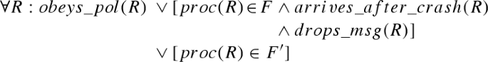
  Correct processors: Observe that, due to the design of $\underline{\mathcal {S'}}_{\mathcal {A}, pol, \delta {}, \mu {}}$ and $T_{C\rightarrow R}$, variable $queue$ in $ex$ represents the queue state of $ru$. Every receive event in $ru$ occurring while the processor is idle corresponds to either a type (a) or a type (e) action. In every such action, a scheduling decision according to $pol$ is made (Line 11) and $T_{C\rightarrow R}$ ensures that either a drop event (type (e) action) or a job (type (a) action) according to the output of that scheduling decision is created. Crashing processors: Fix some processor $p \in F$ and let $ac^{last}$ be the first action $ac$ on $p$ satisfying $is\_last(ac)$. For all actions on $p$ up to (and including) $ac^{last}$ (or for all actions, if no such $ac^{last}$ exists), the transformation rules are equivalent to those for correct processors and, thus, the above reasoning applies for all receive events on $p$ prior to $J^{last}$ (cf. Observation 15). The transformation rules for messages received on crashing processors (Sect. 5.8) ensure that all receive events satisfy either $obeys\_pol(R)$ (if received during $J^{last}$: no scheduling decision—neither job start nor message drop—is made) or $arrives\_after\_crash(R)$ and $drops\_msg(R)$ (if received after $J^{last}$ has finished processing: the message is dropped immediately).

• 

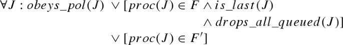
  Correct processors: The same reasoning as in the previous point applies: Every job in $ru$ finishing corresponds to a type (c) or (d) action in $ex$ in which the (finished-processing) message representing that job arrives. Both of these actions cause a scheduling decision (Line 11) to be made on $queue$ (which corresponds to $ru$’s queue state), and corresponding drop events and/or a corresponding job (only type (c) actions) are created by $T_{C\rightarrow R}$. Crashing processors: For all jobs before $J^{last}$, the same reasoning as for correct processors applies. The transformation rules ensure that all messages that have not been processed or dropped before get dropped at $end(J^{last})$.

• 

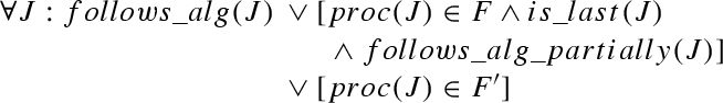
  Correct processors: Let $ac$ be the type (a) or (c) action corresponding to $J$. $ac$ executes all state transitions of $\mathcal {A}$ (Line 17) for either $msg(ac)$ (type (a) action) or some message from the queue (type (c) action) and the current hardware clock time, plus some additional operations that only affect variables $queue$ and $idle$ and (finished-processing) messages. Thus, $T_{C\rightarrow R}$’s choice of $HC(J)$, $msg(J)$ and $trans(J)$ ensure that $trans(J)$ conforms to algorithm $\mathcal {A}$. Crashing processors: For all jobs before $J^{last}$, the same reasoning as for the correct processor applies. Since $J^{last}$ corresponds to either $ac^{last}$ (which also satisfies $follows\_alg\_partially$) or to some earlier type (a) or (c) action (which satisfies $follows\_alg$), $follows\_alg\_partially(J^{last})$ is satisfied.

• $\forall J: is\_timely\_job(J, \mu ^-_{}, \mu ^+_{}) \vee [proc(J) \in F']$ Correct processors: $T_{C\rightarrow R}$ ensures that $duration(J)$ equals the transmission time of the (finished-processing) message sent by the action $ac$ corresponding to job $J$. Since $arrives\_timely(m_t)$ holds for (finished-processing) messages $m_t$ in $ex$, there are exactly $\tilde{\mu }_{(\ell )}{}$ hardware clock time units between the sending and the reception of the (finished-processing) message sent by $ac$ (see Line 19 of $\underline{\mathcal {S}}_{\mathcal {A}, pol, \mu {}}$). By Lemma 4, this corresponds to some real-time interval within $[\mu ^-_{(\ell )}, \mu ^+_{(\ell )}]$. Since $\ell$ equals the number of ordinary messages sent in $J$ (see Line 18 of the algorithm and the transformation rules for type (a) and (c) actions in $T_{C\rightarrow R}$), $is\_timely\_job(J, \mu ^-_{}, \mu ^+_{})$ holds. Crashing processors: For all jobs before $J^{last}$, the same reasoning as for the correct processor applies. If $ac$, the action corresponding to $J^{last}$, was able to successfully send a (finished-processing) message, the above reasoning holds for $J^{last}$ as well. Otherwise, the transformation rules (Sect. 5.3) ensure that $J^{last}$ takes exactly $\mu ^-_{(\ell )}$ time units, with $\ell$ denoting the number of ordinary messages that would have been sent in the non-crashing case, as required by $is\_timely\_job$.

• $\forall p: bounded\_drift(p, \rho ) \vee [proc(J) \in F']$ Follows from the definition that $HC^{ru}_p = HC^{ex}_p$ and the fact that the corresponding $bounded\_drift$ condition holds in $ex$. $\square$

5.11 Transformation proof

Theorem 16

Let $\underline{s}= (n, [\underline{\delta }^-, \underline{\delta }^+])$ be a classic system, and let $\mathcal {P}$ be a simulation-invariant problem. If

• the algorithm $\mathcal {A}$ solves problem $\mathcal {P}$ in some real-time system $s= (n, [\delta ^-_{}, \delta ^+_{}], [\mu ^-_{}, \mu ^+_{}])$ with some scheduling/admission policy $pol$ under failure model $f$-$f'$-$\rho$ [A1] ⁸ and

• conditions Cond1’, Cond2’ and Cond3’ (see Sect. 5.7) hold,

then the algorithm $\underline{\mathcal {S'}}_{\mathcal {A}, pol, \delta {}, \mu {}}$ solves $\mathcal {P}$ in $\underline{s}$ under failure model $f$-$f'$-$\rho$.

Proof

Let $ex$ be such an execution of $\underline{\mathcal {S'}}_{\mathcal {A}, pol, \delta {}, \mu {}}$ in $\underline{s}$ under failure model $f$-$f'$-$\rho$ [D1]. By Lemmas 13 and 14 as well as conditions Cond1’, Cond2’ and Cond3’, $ru= T_{C\rightarrow R}(ex)$ is a valid rt-run of $\mathcal {A}$ in $s$ with scheduling/admission policy $pol$ under failure model $f$-$f'$-$\rho$ [L1].

As $\mathcal {A}$ is an algorithm solving $\mathcal {P}$ in $s$ with policy $pol$ under failure model $f$-$f'$-$\rho$ ([A1]) and $ru$ is a valid rt-run of $\mathcal {A}$ in $s$ with policy $pol$ conforming to failure model $f$-$f'$-$\rho$ ([L1]), $ru$ satisfies $\mathcal {P}$ (cf. Sect. 4.4) [L2].

To show that $ex$ satisfies $\mathcal {P}$, we must show that $tr' \in \mathcal {P}$ holds for every st-trace $tr'$ of $ex$. Let $tr'$ be an st-trace of $ex$, and let $tr'/t$ be the list of all $transition$ st-events in $tr'$ [D2]. We will construct some $transition$ list $tr/t$ from $tr'/t$ by sequentially performing these operations for the $transition$ st-events of all non-Byzantine processors:

• 1. Remove the variables $queue$ and $idle$ from all states.

• 2. Remove any $transition$ st-events that only manipulate $queue$ and/or $idle$. Note that, due to the previous step, these st-events satisfy $oldstate = newstate$.

Since $\mathcal {P}$ is a simulation-invariant problem, there is some finite set $\mathcal {V}$ of variable names, such that $\mathcal {P}$ is a predicate on global states restricted to $\mathcal {V}$ and the sequence of $input$ st-events (cf. Definition 3). Since variables $queue$ and $idle$ in algorithm $\underline{\mathcal {S'}}_{\mathcal {A}, pol, \delta {}, \mu {}}$ could be renamed arbitrarily, we can assume w.l.o.g. that $queue \not \in \mathcal {V}$ and $idle \not \in \mathcal {V}$. Examining the list of operations in the definition of $tr$ reveals that $gstates(tr')|_\mathcal {V}= gstates(tr)|_\mathcal {V}$, for every $tr$ having the same $transition$ st-events as $tr/t$ [L3].

We now show that $tr/t$ is the $transition$ sequence of some st-trace of $ru$ where all transitions happen at the very beginning of each job.

• Every job in $ru$ on a non-Byzantine processor is correctly mapped to $transition$ st-events in $tr/t$: Every job $J$ in $ru$ is based on either a type (a) or a type (c) action $ac$ in $ex$. According to Sect. 4, the $transition$ st-events produced by mapping $ac$ are the same as the st-events produced by mapping $J$, except that the st-events mapped by $ac$ contain the simulation variables. However, they have been removed by the transformation from $tr'/t$ to $tr/t$.

• Every $transition$ st-event in $tr/t$ on a non-Byzantine processor corresponds to a job in $ru$: Every st-event in $tr'/t$ is based on an action $ac$ in $ex$. Since the transformation $tr'/t \rightarrow tr/t$ does not add any st-events, every st-event in $tr/t$ is based on an action $ac$ in $ex$ as well. Since all st-events only modifying $queue$ and $idle$ have been removed, $tr/t$ only contains the st-events corresponding to some type (a) or (c) action in $ex$. The st-events in $tr'/t$ contain the $transition$ st-events of $\mathcal {A}$-process_message(msg, current_hc) and additional steps taken by the simulation algorithm. The transformation from $tr'/t$ to $tr/t$ ensures that these additional steps (and only these) are removed. Thus, the remaining st-events in $tr$ correspond to the job $J$ corresponding to $ac$.

• For Byzantine processors, recall (Sect. 5.3) that the actions in $ex$ and their corresponding jobs in $ru$ perform exactly the same state transitions.

Following the rules in Sect. 4.4, an st-trace $tr$ for $ru$ where all transitions happen at the very beginning of each job must exist. Thus, we can conclude that $tr/t$ is the $transition$ sequence of some st-trace $tr$ of $ru$ [L4]. W.r.t. $input$ st-events, note that the same $input$ st-events occur in $tr$ and $tr'$, except for Byzantine processors, which might receive dummy input messages in $ru$ (and, thus, in $tr$) that are missing in $ex$ (and, thus, in $tr'$), cf. Sect. 5.8. Cond1’, however, ensures that $\mathcal {P}$ does not care about input messages sent to Byzantine processors.

As $\mathcal {A}$ solves $\mathcal {P}$ in $s$ with policy $pol$ under failure model $f$-$f'$-$\rho$ ([A1]), $ru$ is an rt-run of $\mathcal {A}$ in $s$ with policy $pol$ under failure model $f$-$f'$-$\rho$ ([L1]), and $tr$ is an st-trace of $ru$, $tr\in \mathcal {P}$ [L5]. Since $gstates(tr')|_\mathcal {V}= gstates(tr)|_\mathcal {V}$ ([L3,L4]), $tr\in \mathcal {P}$ ([L5]), and $\mathcal {P}$ is a simulation-invariant problem, $tr' \in \mathcal {P}$ [L6].

As this ([L6]) holds for every st-trace $tr'$ of every execution $ex$ of $\underline{\mathcal {S'}}_{\mathcal {A}, pol, \delta {}, \mu {}}$ in $\underline{s}$ under failure model $f$-$f'$-$\rho$ ([D1,D2]), $\underline{\mathcal {S'}}_{\mathcal {A}, pol, \delta {}, \mu {}}$ solves $\mathcal {P}$ in $\underline{s}$ under failure model $f$-$f'$-$\rho$. $\square$

6 Running classic algorithms in the real-time model

When running a real-time model algorithm in a classic system, as shown in the previous section, the st-traces of the simulated rt-run and the ones of the actual execution are very similar: Ignoring variables solely used by the simulation algorithm, it turns out that the same state transitions occur in the rt-run and in the corresponding execution.

Unfortunately, this is not the case for transformations in the other direction, i.e., running a classic model algorithm in a real-time system: The st-traces of a simulated execution are usually not the same as the st-traces of the corresponding rt-run. While all state transitions of some action $ac$ at time $t$ always occur at this time, the transitions of the corresponding job $J$ take place at some arbitrary time between $t$ and $t + duration(J)$. Thus, there could be algorithms that solve a given problem in the classic model, but fail to do so in the real-time model.

Fortunately, however, it is possible to show that if some algorithm solves some problem $\mathcal {P}$ in some classic system, the same algorithm can be used to solve a variant of $\mathcal {P}$, denoted ${\mathcal {P}}^*_{\mu ^+_{}}$, in some corresponding real-time system, where the end-to-end delay bounds ${\varDelta }^-$ and ${\varDelta }^+$ of the real-time system equal the message delay bounds $\underline{\delta }^-$ and $\underline{\delta }^+$ of the simulated classic system. For the fault-free case, this has been already been shown [26].

The key to this transformation is a very simple simulation: Let ${\mathcal {S}_{\underline{\mathcal {A}}}}$ (= Algorithm 3) be an algorithm for the real-time model, comprising exactly the same initial states and transition function as a given classic model algorithm $\underline{\mathcal {A}}$.

The major problem here is the circular dependency of the algorithm $\underline{\mathcal {A}}$ on the real end-to-end delays and vice versa: On one hand, the classic model algorithm $\underline{\mathcal {A}}$ running atop of the simulation might need to know the simulated message delay bounds $[\underline{\delta }^-,\underline{\delta }^+]$, which are just the end-to-end delay bounds $[{\varDelta }^-,{\varDelta }^+]$ of the underlying simulation. Those end-to-end delays, on the other hand, involve the queuing delay $\omega$ and are thus dependent on (the message pattern of) $\underline{\mathcal {A}}$ and hence on $[\underline{\delta }^-,\underline{\delta }^+]$.

This issue, already discussed in Sect. 2.2, can be resolved by fixing the failure model $\mathcal {C}= f-f'-\rho$, some scheduling/admission policy $pol$, assuming some message delay bounds $[\underline{\delta }^-,\underline{\delta }^+] = [{\varDelta }^-, {\varDelta }^+]$, considered as unvalued parameters, and conducting a worst-case end-to-end delay analysis of the transformed algorithm ${\mathcal {S}_{\underline{\mathcal {A}}}}$ in order to develop a fixed point equation for the resulting end-to-end delay bounds, i.e., $[{\varDelta }^-{}, {\varDelta }^+{}] =\,F_{\mathcal {A},\mathcal {C},pol}([\delta ^-_{}, \delta ^+_{}],\,[\mu ^-_{}, \mu ^+_{}], [{\varDelta }^-{}, {\varDelta }^+{}])$. If this equation can be solved, resulting in a feasible solution ${\varDelta }^-\le {\varDelta }^+$, these bounds can be safely assigned to the algorithm parameters $[\underline{\delta }^-, \underline{\delta }^+]$.

Definition 17

[26] Let $tr$ be an st-trace based on some execution $ex$ or rt-run $ru$. A $\mu ^+_{}$-shuffle of $tr$ is constructed by moving $transition$ st-events in $tr$ at most $\mu ^+_{(\ell )}$ time units into the future. These operations must preserve causality in a sense similar to the well-known happened before relation [10]:

• The order of $transition$ st-events on the same processor must not change.

• The order of $transition$ st-events connected by a message must not change: Let $s_1 \rightarrow s_2$ be a state transition occurring on some processor $p$ right before $p$ sends some message $m$. Let $s_3 \rightarrow s_4$ be a state transition occurring on some processor $q$ in the action or job triggered by $m$ on $q$. In the shuffled st-trace, $(s_1 \rightarrow s_2) \prec (s_3 \rightarrow s_4)$ must still hold.

Every st-event may be shifted by a different value $v$, $0 \le v \le \mu ^+_{(\ell )}$. In addition, $input$ st-events may be moved arbitrarily far into the past.⁹

${\mathcal {P}}^*_{\mu ^+_{}}$ is the set of all $\mu ^+_{}$-shuffles of all st-traces of $\mathcal {P}$.¹⁰

Example 18

Consider the classic Mutual Exclusion problem for $\mathcal {P}$, and assume that there is some algorithm $\underline{\mathcal {A}}$ solving this problem in the classic model. When running ${\mathcal {S}_{\underline{\mathcal {A}}}}$ in the real-time model, the situation depicted in Fig. 8 can occur: As the actual state transitions can occur at any time during a job (marked as ticks in the figure), it may happen that, at a certain time (marked as a dotted vertical line), $p$ has entered the critical section although $q$ has not left yet. This situation arises because ${\mathcal {P}}^*_{\mu ^+_{}}$ is a weaker problem than mutual exclusion; in other words, ${\mathcal {S}_{\underline{\mathcal {A}}}}$ only solves mutual exclusion with up to $\mu ^+_{}$-second overlap.

On the other hand, assume that $\mathcal {P}$ is the 3-second gap mutual exclusion problem, defined by the classic mutual exclusion properties and the additional requirement that all processors must have left the critical section for more than 3 seconds before the critical section can be entered again by some processor. In that case, ${\mathcal {P}}^*_{\mu ^+_{}}$ with $\mu ^+_{} = 2$ seconds is the $1$-second gap mutual exclusion problem. Thus, if $\underline{\mathcal {A}}$ solves the $3$-second gap mutual exclusion problem, running ${\mathcal {S}_{\underline{\mathcal {A}}}}$ would solve mutual exclusion in a real-time model where $\mu ^+_{} \le 3$ seconds.

Nevertheless, it turns out that most classic mutual exclusion algorithms work correctly in the real-time model. The reason is that these algorithms in fact solve a stronger problem: Let $\mathcal {P}$ be causal mutual exclusion, defined by the classic mutual exclusion properties and the additional requirement that every state transition in which a processor enters a critical section must causally depend on the last exit. Since shuffles must not violate causality, in this case, ${\mathcal {P}}^*_{\mu ^+_{}}= \mathcal {P}$, and the same algorithm used for some classic system can also be used in a real-time system with a feasible end-to-end delay assignment. $\square$

Fig. 8

Example of a classic model mutual exclusion algorithm (top) running in the real-time model (bottom)

6.1 Conditions

Theorem 22 will show that the following conditions are sufficient for the transformation to work in the fault-tolerant case:

• Cond1 There is a feasible end-to-end delay assignment $[{\varDelta }^-, {\varDelta }^+] = [\underline{\delta }^-, \underline{\delta }^+]$.

• Cond2 The scheduling/admission policy (a) only drops irrelevant messages and (b) schedules input messages in FIFO order. More specifically, (a) only messages that would have caused a job $J$ with a NOP state transition are allowed to be dropped. For example, these could be messages that obviously originate from a faulty sender or, in round-based algorithms, late messages from previous rounds. (b) If input messages $m_1$ and $m_2$ are in the queue and $m_1$ has been received before $m_2$, then $m_2$ must not be dropped or processed before $m_1$ has been dropped or processed.

• Cond3 The algorithm tolerates late timer messages, and the scheduling policy ensures that timer messages get processed soon after being received. In the classic model, a timer message scheduled for hardware clock time $T$ gets processed at time $T$. In the real-time model, on the other hand, the message arrives when the hardware clock reads $T$, but it might get queued if the processor is busy. Still, an algorithm designed for the classic model might depend on the message being processed exactly at hardware clock time $T$. Thus, either (a) the algorithm must be tolerant to timers being processed later than their designated arrival time or (b) the scheduling policy must ensure that timer messages do not experience queuing delays—which might not be possible, since we assume a non-idling and non-preemptive scheduler. Cond3 is a combination of those options: The algorithm tolerates timer messages being processed up to $\alpha$ real-time units after the hardware clock read $T$, and the scheduling policy ensures that no timer message experiences a queuing delay of more than $\alpha$. Options (a) and (b) outlined above correspond to the extreme cases of $\alpha = \infty$ and $\alpha = 0$. These requirements can be encoded in failure models: $f$-$f'$-$\rho$+latetimers$_{\alpha }$, a failure model on executions in the classic model, is weaker than $f$-$f'$-$\rho$ (i.e., $ex\in f-f'-\rho \,\Rightarrow ex\in f-f'-\rho +\text {latetimers}_{\alpha }$), since timer messages may arrive late by at most $\alpha$ seconds in the former. On the other hand, $f$-$f'$-$\rho$+precisetimers$_{\alpha }$, a failure model on rt-runs in the real-time model that restricts timer message queuing by the scheduler to at most $\alpha$ seconds, is stronger than $f$-$f'$-$\rho$ (i.e., $ru\in f-f'-\rho +\text {precisetimers}_{\alpha } \Rightarrow ru\in f-f'-\rho$). See Sect. 4.3 for the formal definition of these models.

6.2 The transformation $T_{R\rightarrow C}$ from rt-runs to executions

As shown in Fig. 9, the proof works by transforming every rt-run of ${\mathcal {S}_{\underline{\mathcal {A}}}}$ into a corresponding execution of $\underline{\mathcal {A}}$. By showing that (a) this execution is an admissible execution of $\underline{\mathcal {A}}$ (w.r.t. $f$-$f'$-$\rho$+latetimers$_{\alpha }$) and (b) the execution and the rt-run have (roughly) the same state transitions, the fact that the rt-run satisfies ${\mathcal {P}}^*_{\mu ^+_{}}$ can be derived from the fact that the execution satisfies $\mathcal {P}$. This transformation, $ex= T_{R\rightarrow C}(ru)$, works by

• mapping each job $J$ in $ru$ to an action $ac$ in $ex$, with $time(ac) = begin(J)$,

• mapping each drop event $D$ in $ru$ to a NOP action $ac$ in $ex$,

• setting $HC^{ex}_p = HC^{ru}_p$ for all $p$.

• Receive events in $ru$ are ignored.

The following sections will show the correctness of the transformation.

Fig. 9

Proof outline (Theorem 22)

6.3 Validity of the constructed execution

Lemma 19

If $ru$ is a valid rt-run of ${\mathcal {S}_{\underline{\mathcal {A}}}}$, $ex= T_{R\rightarrow C}(ru)$ is a valid execution of $\underline{\mathcal {A}}$.

Proof

EX1–6 (cf. Sect. 4.1) are satisfied in $ex$: EX1 follows from RU1 by ordering the actions like their corresponding jobs and drop events. EX2 follows from RU2 and the fact that the order of jobs in $ru$ corresponds to the order of actions in $ex$, that the transition sequence is not changed and that the “correct” state is chosen for actions corresponding to drop events. EX3 is a direct consequence of RU3 and the fact that both $ru$ and $ex$ run the same algorithm (i.e., use the same initial state). Since $ru$ and $ex$ use the same hardware clocks, RU4 suffices to satisfy EX4. EX5 follows directly from RU5, and EX6 follows from RU6. Thus, $ex$ is a valid execution of $\underline{\mathcal {A}}$. $\square$

Lemma 20

For every message $m$ in $ex$, the message delay $\underline{\delta }_m$ is equal to the end-to-end delay ${\varDelta }_{m'}$ of its corresponding message $m'$ in $ru$.

Proof

By construction of $ex$, the sending time of every message stays the same ($time(ac) = begin(J)$, with $ac$ and $J$ being the sending action/job; recall that message delays are measured from the start of the sending job). For dropped messages, the drop time in $ru$ equals the receiving/processing time in $ex$ ($time(ac) = time(D)$, with $ac$ being the processing action and $D$ being the drop event). For other messages, the processing time in $ru$ equals the receiving/processing time in $ex$ ($time(ac) = begin(J)$, with $ac$ being the processing action and $J$ being the processing job). $\square$

6.4 Failure model compatibility

Lemma 21

Let $\underline{s}$ and $s$ be a classic and a real-time system, let $\mathcal {A}$ be a real-time model algorithm, and let $ru$ be an rt-run of $\mathcal {A}$ in system $s$ under failure model $f$-$f'$-$\rho$+precisetimers$_{\alpha }$.

If Cond1, Cond2 and Cond3 hold, $ex= T_{R\rightarrow C}(ru)$ conforms to failure model $f$-$f'$-$\rho$+latetimers$_{\alpha }$ in system $\underline{s}$.

Proof

Lemma 19 has shown that $ex$ is a valid execution of $\underline{\mathcal {A}}$. The following conditions of $f$-$f'$-$\rho$+latetimers$_{\alpha }$, as specified in Sect. 4.3, are satisfied:

• $\forall m_o: is\_timely\_msg(m_o, \underline{\delta }^-{}, \underline{\delta }^+{})$ Follows from Lemma 20 and the fact that Cond1 guarantees a feasible assignment (i.e., $[\underline{\delta }^-, \underline{\delta }^+] = [{\varDelta }^-{}, {\varDelta }^+{}]$).

• $\forall m_t: arrives\_timely(m_t) \vee is\_late\_timer(m_t, \alpha ) \vee [proc(m_t) \in F']$ Let $t$ denote $HC^{-1}_{proc(m_t)}(sHC(m_t))$, i.e., the real time by which timer $m_t$ should arrive. $gets\_processed\_precisely(m_t,\alpha )$ ensures that the job or drop event taking care of $m_t$ starts at most $\alpha$ real-time units after $t$. Due to the transformation rules of $T_{R\rightarrow C}$, this job or drop event is transformed into an action $ac$ receiving and processing $m_t$ and occurring at the same time as the job or drop event. Thus, $is\_late\_timer(m_t, \alpha )$ is satisfied.

• $\forall ac:$ either

• (a) $follows\_alg(ac)$ or

• (b) $proc(ac) \in F \wedge is\_last(ac)$ ${}\wedge follows\_alg\_partially(ac)$ or

• (c) $proc(ac) \in F \wedge arrives\_after\_crash(ac)$ or

• (d) $[proc(ac) \in F']$

Correct processors: All jobs in $ru$ on $p$ adhere to the algorithm. The corresponding actions in $ex$ occur at the same hardware clock time, process the same message and have the same state transition sequence. Thus, (a), $follows\_alg(ac)$, holds for them as well. W.r.t. drop events, Cond2 ensures that only messages that would have caused a NOP state transition may be dropped by $pol$. Due to the $\forall R/J: obeys\_pol(R)/(J)$ conditions and RU8, drop events occurring on non-faulty processors must conform to $pol$. “Would have caused a NOP state transition” means that the algorithm returns a NOP state transition for the current (message, hardware clock, state) tuple. Thus, the action $ac$ corresponding to this drop event satisfies (a), $follows\_alg(ac)$.

Before the processor crashes: The same arguments hold for all jobs $J \prec J^{last}$ on $p$ and all drop events before $J^{last}$. Thus, (a) also holds for their corresponding actions.

During the crash: For $J = J^{last}$, the definition of $follows\_alg\_partially(ac)/(J)$ directly translates to the corresponding action $ac^{last}$. Since there are no jobs $J \succ J^{last}$ on $p$, only actions based on drop events can occur in $p$ after $ac^{last}$, causing $ac^{last}$ to satisfy $is\_last(ac^{last})$. Thus, $ac^{last}$ satisfies (b).

After the processor crashes: By definition of $is\_last(J)$, no jobs occur in $ru$ after a processor has crashed. Drop events occurring after a processor has crashed need not (and usually will not) obey the scheduling policy: Messages received and queued before the last job are dropped directly after that job (see predicate $drops\_all\_queued(J)$), and messages received afterwards are dropped immediately (see predicate $arrives\_after\_crash(R)$). Since $ac^{last} \prec ac$ holds for all actions $ac$ corresponding to such drop events (on some processor $p$), (c), $arrives\_after\_crash(ac)$, is satisfied.

• $\forall p: bounded\_drift(p, \rho ) \vee [p \in F']$ Follows from the equivalent condition in $f$-$f'$-$\rho$+precisetimers$_{\alpha }$ and the fact that $T_{R\rightarrow C}$ ensures that $HC^{ex}_p = HC^{ru}_p$ for all $p$. $\square$

6.5 Transformation proof

Theorem 22

Let $s= (n, [\delta ^-_{}, \delta ^+_{}], [\mu ^-_{}, \mu ^+_{}])$ be a real-time system, $pol$ be a scheduling/admission policy and $\mathcal {P}$ be a problem. If

• the algorithm $\underline{\mathcal {A}}$ solves $\mathcal {P}$ in some classic system $\underline{s}= (n, [\underline{\delta }^-, \underline{\delta }^+])$ under some failure model $f$-$f'$-$\rho$+latetimers$_{\alpha }$ [A1],

• conditions Cond1, Cond2 and Cond3 (see Sect. 6.1) hold,

then the algorithm ${\mathcal {S}_{\underline{\mathcal {A}}}}$ solves ${\mathcal {P}}^*_{\mu ^+_{}}$ in $s$ under failure model $f$-$f'$-$\rho$+precisetimers$_{\alpha }$ with scheduling/admission policy $pol$.

Proof

Let $ru$ be an rt-run of ${\mathcal {S}_{\underline{\mathcal {A}}}}$ in $s$ under failure model $f$-$f'$-$\rho$+precisetimers$_{\alpha }$ with scheduling/admission policy $pol$ [D1]. Let $ex= T_{R\rightarrow C}(ru)$. As $\underline{\mathcal {A}}$ solves $\mathcal {P}$ in $\underline{s}$ under failure model $f$-$f'$-$\rho$+latetimers$_{\alpha }$ ([A1]) and $ex$ is a valid execution of $\underline{\mathcal {A}}$ (Lemma 19) conforming to failure model $f$-$f'$-$\rho$+latetimers$_{\alpha }$ in $\underline{s}$ (Lemma 21), $ex$ satisfies $\mathcal {P}$ [L1].

To show that $ru$ satisfies ${\mathcal {P}}^*_{\mu ^+_{}}$, we must show that every st-trace $tr'$ of $ru$ is a $\mu ^+_{}$-shuffle of an st-trace $tr$ of $ex$. Let $tr'$ be an st-trace of $ru$ [D2]. We can construct $tr$ from $tr'$ as follows:

• Move the time of every $transition$ st-event back to the begin time of the job corresponding to this st-event.

• Move the time of every $input$ st-event forward so that it has the same time as the begin time of the job processing the message.

Since $pol$ ensures that input messages are processed in FIFO order (Cond2), the above operations are an inverse subset of the $\mu ^+_{}$-shuffle operations (see Definition 17); thus, $tr'$ is a $\mu ^+_{}$-shuffle of $tr$ [L2]. Still, we need to show that $tr$ is an st-trace of $ex$:

• Every action in $ex$ is correctly mapped to st-events in $tr$: Every job $J$ in $ru$ is mapped to an action $ac$ in $ex$ and a sequence of $transition$ st-events in $tr$ (plus at most one $input$ st-event corresponding to $J$’s receive event). There are two differences in the mapping of some job $J$ to st-events and the corresponding action $ac$ to st-events:

  • The $transition$ st-events all occur at the same time $time(ac)$ when mapping an action. The construction of $tr$ ensures that this is the case.

  • If $msg(ac)$ is an input message, the corresponding $input$ st-event occurs at the same time as the action processing it. Since $ru$ satisfies RU6, there is also such an $input$ st-event in $tr'$, and, thus, in $tr$. The construction of $tr$ ensures that this $input$ st-event has the correct position in $tr$.

  Every drop event $D$ in $ru$ is mapped to a NOP action $ac$, i.e., an action with $trans(ac) = [s]$, $s := oldstate(ac) = newstate(ac)$, in $ex$. Neither $D$ nor $ac$ get mapped to any $transition$ st-event. If the dropped message was an input message, the same reasoning as above applies w.r.t. the $input$ st-event.

• Every st-event in $tr$ belongs to an action in $ex$: Every st-event in $tr'$ (and, thus, every corresponding st-event in $tr$) is based on either a job, an input message receive event or a drop event in $ru$. By construction of $ex$, every job and every drop event is mapped to one action, requiring the same amount of $transition$ st-events. Every input message receive event in $ru$ results in an $input$ st-event. This $input$ st-event belongs to the action processing it.

Thus, we can conclude that $tr$ is an st-trace of $ex$ [L3]. As $ex$ satisfies $\mathcal {P}$ ([L1]), this ([L3]) implies that $tr\in \mathcal {P}$ [L4]. Since $tr'$ is a $\mu ^+_{}$-shuffle of $tr$ ([L2]) and $tr\in \mathcal {P}$ ([L4]), Definition 17 states that $tr' \in {\mathcal {P}}^*_{\mu ^+_{}}$ [L5].

As this ([L5]) holds for every st-trace $tr'$ of every rt-run $ru$ of ${\mathcal {S}_{\underline{\mathcal {A}}}}$ in $s$ under failure model $f$-$f'$-$\rho$+precisetimers$_{\alpha }$ with scheduling/admission policy $pol$ ([D1, D2]), ${\mathcal {S}_{\underline{\mathcal {A}}}}$ solves ${\mathcal {P}}^*_{\mu ^+_{}}$ in $s$ under failure model $f$-$f'$-$\rho$+precisetimers$_{\alpha }$ with scheduling/admission policy $pol$. $\square$

7 Examples

In previous work [26], the fault-free variant of the transformations were applied to the problem of terminating clock synchronization; the results are summarized in Sect. 7.1.

To illustrate the theorems established in this work, we apply them to the Byzantine Generals problem—a well-known agreement problem that also incorporates failures. Section 7.2 will demonstrate that the comparatively simple worst-case end-to-end delay analysis made possible by our transformations is competitive with respect to the optimal solution.

7.1 Terminating clock synchronization

In the absence of clock-drift and failures, clock synchronization is a one-shot problem: Once the clocks are synchronized to within some bound $\gamma$, they stay synchronized forever. In the classic system model, a tight bound of $\gamma = (\underline{\delta }^+-\underline{\delta }^-)(1-\frac{1}{n})$ of the clock precision (also termed skew) is well-known [13]. Applying our transformations to this problem yields the following results [26]:

Lower Bound: The impossibility of achieving a precision better than $(\underline{\delta }^+-\underline{\delta }^-)(1-\frac{1}{n})$ translates to an impossibility of a precision better than $(\delta ^+_{(1)}-\delta ^-_{(1)})(1-\frac{1}{n})$ in the real-time model (cf. Cond2’ in Sect. 5 and Theorem 11 of [26]).

Informally speaking, the argument goes as follows: Assume by way of contradiction that an algorithm $\mathcal {A}$ achieving a precision better than $(\delta ^+_{(1)}-\delta ^-_{(1)})(1-\frac{1}{n})$ in the real-time model exists. We can now use the transformation presented in [26], which is essentially a simple, non-fault-tolerant variant of this paper’s Sect. 5, to construct a classic algorithm $\underline{\mathcal {S'}}_{\mathcal {A}, pol, \delta {}, \mu {}}$ achieving a precision better than $(\underline{\delta }^+-\underline{\delta }^-)(1-\frac{1}{n})$. Since the latter is known to be impossible, no such algorithm $\mathcal {A}$ can exist.

Upper Bound: Let $\underline{\mathcal {A}}$ be the algorithm from [13] achieving a precision of $(\underline{\delta }^+-\underline{\delta }^-)(1-\frac{1}{n})$ in the classic model. Since $\underline{\mathcal {A}}$ depends on $\underline{\delta }^-$ and $\underline{\delta }^+$, ${\mathcal {S}_{\underline{\mathcal {A}}}}$ depends on ${\varDelta }^-$ and ${\varDelta }^+$ (cf. Cond1 in Sect. 6). However, due the simplicity of the algorithm, the message pattern created by $\underline{\mathcal {A}}$ (and, thus, by ${\mathcal {S}_{\underline{\mathcal {A}}}}$) does not depend on the actual values of $\underline{\delta }^-$ and $\underline{\delta }^+$ (or ${\varDelta }^-$ and ${\varDelta }^+$, respectively). When running ${\mathcal {S}_{\underline{\mathcal {A}}}}$, the worst-case with respect to queuing times occurs when $n-1$ messages arrive simultaneously at one processor that has just started broadcasting its clock value. Thus, ${\varDelta }^+$ can be bounded by $\delta ^+_{(n-1)} + \mu ^+_{(n-1)} + (n-2)\mu ^+_{(0)}$ (cf. Theorem 10 of [26]). Since every action of $\underline{\mathcal {A}}$ sends either $0$ or $n-1$ messages, ${\varDelta }^-$ in ${\mathcal {S}_{\underline{\mathcal {A}}}}$ turns out to be $\delta ^-_{(n-1)}$. Since $(\underline{\delta }^+-\underline{\delta }^-)(1-\frac{1}{n})$ translates to $({\varDelta }^+-{\varDelta }^-)(1-\frac{1}{n})$ during the transformation, the resulting algorithm ${\mathcal {S}_{\underline{\mathcal {A}}}}$ can synchronize clocks to within $(\delta ^+_{(n-1)} + \mu ^+_{(n-1)} + (n-2)\mu ^+_{(0)} - \delta ^-_{(n-1)})(1-\frac{1}{n})$.

Thus, applying these transformations leaves a gap in between what has been a tight bound in the classic model. As a consequence, more intricate algorithms are required to achieve optimal precision in the real-time model. In fact, [26] also shows that a tight precision bound of $(\delta ^+_{(1)}-\delta ^-_{(1)})(1-\frac{1}{n})$ can be obtained by using an algorithm specifically designed for the real-time model. On the other hand, the transformed algorithm is still quite competitive and much easier to obtain and to analyze.

7.2 The Byzantine generals

We consider the Byzantine Generals problem [11], which is defined as follows: A commanding general must send an order to his $n - 1$ lieutenant generals such that

• IC1 All loyal lieutenants obey the same order.

• IC2 If the commanding general is loyal, then every loyal lieutenant obeys the order he sends.

In the context of computer science, generals are processors, orders are binary values and loyal means fault-free. It is well-known that $f$ Byzantine faulty processors can be tolerated if $n > 3f$. The difficulty in solving this problem lies in the fact that a faulty processor might send out asymmetric information: The commander, for example, might send value $0$ to the first lieutenant, value $1$ to the second lieutenant and no message to the remaining lieutenants. Thus, the lieutenants (some of which might be faulty as well) need to exchange information afterwards to ensure that IC1 is satisfied.

Lamport et al. [11] presents an “oral messages” algorithm, which we will call $\underline{\mathcal {A}}$: Initially (round $0$), the value from the commanding general is broadcast. Afterwards, every round basically consists of broadcasting all information received in the previous round. After round $f$, the non-faulty processors have enough information to make a decision that satisfies IC1 and IC2.

What makes this algorithm interesting in the context of this paper is the fact that (a) it is a synchronous round-based algorithm and (b) the number of messages exchanged during each round increases exponentially: After receiving $v$ from the commander in round $0$, lieutenant $p$ sends “$p: v$” to all other lieutenants in round $1$ (and receives such messages from the others).¹¹ In round $2$, it relays those messages, e.g., processor $q$ would send “$q: p: v$”, meaning: “processor $q$ says: (processor $p$ said: (the commander said: $v$))”, to all processors except $p$, $q$ and the commander. More generally, in round $r\ge 2$, every processor multicasts $\#_S=(n-2)\cdots (n-r)$ messages, each sent to $n-r-1$ recipients, and receives $\#_R=(n-2)\cdots (n-r-1)$ messages.¹²

Implementing synchronous rounds in the classic model is straightforward when the clock skew is bounded; for simplicity, we will hence assume that the hardware clocks are perfectly synchronized. At the beginning of a round (at some hardware clock time $t$), all processors perform some computation, send their messages and set a timer for time $t + \underline{\delta }^+$, after which all messages for the current round have been received and processed and the next round can start.

We model these rounds as follows: The round start is triggered by a timer message. The triggered action, labeled as $C$, (a) sets a timer for the next round start and (b) initiates the broadcasts (using a timer message that expires immediately). The broadcasts are modeled as $\#_S$ actions on each processor (labeled as $S$), connected by timer messages that expire immediately. Likewise, the $\#_R$ actions receiving messages are labeled $R$.

Since the algorithm is simple, it is intuitively clear what needs to be done in order to make this algorithm work in the real-time model: We need to determine the longest possible round duration $W$ (in the real-time model), i.e., the maximum time required for any one processor to execute all its $C$, $S$ and $R$ jobs, and replace the delay of the “start next round” timer from $\underline{\delta }^+$ to this value. Figure 10 shows examples of running a round of the algorithm in the real-time model.

Let us take a step back and examine the problem from a strictly formal point of view: Given algorithm $\underline{\mathcal {A}}$, we will try to satisfy Cond1, Cond2 and Cond3, so that the transformation of Sect. 6 can be applied.

For this example, let us restrict our failure model to a set of $f$ processors that produce only benign message patterns, i.e., a faulty processor may crash or modify the message contents arbitrarily, but it must not send additional messages or send the messages at a different time (than a fault-free or crashing processor would). We will denote this restricted failure model as $f^*$ and claim (proof omitted) that the failure model relation established in Theorem 22 also holds for this model, i.e., that a classic algorithm conforming to model $f^*$+latetimers$_{\alpha }$ can be transformed to a real-time algorithm in model $f^*$+precisetimers$_{\alpha }$.

Let us postpone the problem of determining a feasible assignment for $[{\varDelta }^-{},{\varDelta }^+{}]$ (Cond1) until later. Cond2 can be satisfied easily by choosing a suitable scheduling/admission policy. Cond3 deals with timer messages, and this needs some care: Timer messages must arrive “on time” or the algorithm must be able to cope with late timer messages or a little bit of both (which is what factor $\alpha$ in Cond3 is about). In $\underline{\mathcal {A}}$, we have two different types of timer messages: (a) the timer messages initiating the send actions and (b) the timer messages starting a new round.

How can we ensure that $\underline{\mathcal {A}}$ still works under failure model $f^*$+latetimers$_{\alpha }$ (in the classic model)? If the timers for the $S$ jobs each arrive $\alpha$ time units later, the last send action occurs $\#_S \cdot \alpha$ time units after the start of the round instead of immediately at the start of the round. Likewise, if the timer for the round start occurs $\alpha$ time units later, everything is shifted by $\alpha$. To take this shift into account, we just have to set the round timer to $\underline{\delta }^++ (\#_S + 1)\alpha$.

As soon as we have a feasible assignment, Theorem 22 will thus guarantee that ${\mathcal {S}_{\underline{\mathcal {A}}}}$ solves $\mathcal {P}= {\mathcal {P}}^*_{\mu ^+_{}}= \text {IC1} + \text {IC2}$ under failure model $f^*$+precisetimers$_{\alpha }$. For the time being, we choose $\alpha = \mu ^+_{(n-1)}$, so the round timer in ${\mathcal {S}_{\underline{\mathcal {A}}}}$ waits for ${\varDelta }^+{} + (\#_S+1)\mu ^+_{(n-1)}$ time units. This is a reasonable choice: Since the $S$ jobs are chained by timer messages expiring immediately, these timer messages are delayed at least by the duration of the job setting the timer. We will later see that $\mu ^+_{(n-1)}$ suffices.

Returning to Cond1, the problem of determining ${\varDelta }^+{}$ can be solved by a very conservative estimate: Choose ${\varDelta }^+{} = \delta ^+_{(n-1)} + \mu ^+_{(0)} + \#^f_S \cdot \mu ^+_{(n-1)} + (\#^f_R - 1)\mu ^+_{(0)}$, with $\#^f_S$ and $\#^f_R$ denoting the maximum number of send and receive jobs (= the number of such jobs in the last round $f$); this is the worst-case time required for one message transmission, one $C$, all $S$ and all $R$ except for one (= the one processing the message itself). Clearly, the end-to-end delay of one round $r$ message—consisting of transmission plus queuing but not processing—cannot exceed this value if the algorithm executes in a lock-step fashion and no rounds overlap. This is ensured by the following lemma: For all rounds $r$, the following holds: (a) The round timer messages on all processors start processing simultaneously. (b) As soon as the round timer messages starting round $r$ arrive, all messages from round $r-1$ have been processed. Since, for our choice of ${\varDelta }^+{}$, the round timer waits for $\delta ^+_{(n-1)} + (\#^f_S+\#_S+1)\mu ^+_{(n-1)} + \#^f_R \cdot \mu ^+_{(0)}$ time units, it is plain to see that this is more than enough time to send, transmit and process all pending round $r$ messages by choosing a scheduling policy that favors $C$ jobs before $S$ jobs before $R$ jobs. Formally, this can be shown by a simple induction on $r$; for intuition, examine Fig. 10. Considering this scheduling policy and this lemma, it becomes apparent that $\alpha = \mu ^+_{(n-1)}$ was indeed sufficient (see above): A timer for an $S$ job is only delayed until the current $C$ or $S$ job has finished.

Fig. 10

Rounds with durations $W^a$, $W^b$ and $W^c$, critical path highlighted [25]. a $W^a$: message transmission faster than total send job processing. b $W^b$: message transmission slower than total send job. c $W^c$: fast receive job processing

Thus, we end up with an algorithm ${\mathcal {S}_{\underline{\mathcal {A}}}}$ satisfying IC1 and IC2, with synchronous round starts and a round duration of $\delta ^+_{(n-1)} + (\#^f_S+\#_S+1)\mu ^+_{(n-1)} + \#^f_R \cdot \mu ^+_{(0)}$.

7.2.1 Competitive factor

Since the transformation is generic and does not exploit the round structure, the round duration is considerably larger than necessary: Theorem 22 requires one fixed “feasible assignment” for ${\varDelta }^+{}$; thus, we had to choose $\#^f_S$ and $\#^f_R$ instead of $\#_S$ and $\#_R$, which are much smaller for early rounds.

Define $\mu _C:= \mu ^+_{(0)}$, $\mu _R:= \mu ^+_{(0)}$ and $\mu _S:= \mu ^+_{(n-r-1)}$. Since the rounds are disjoint—no messages cross the “round barrier”—and $\underline{\delta }^+{}$/${\varDelta }^+{}$ are only required for determining the round duration, a careful analysis of the transformation proof reveals that the results still hold if $\alpha$, the maximum delay of timer messages, and ${\varDelta }^+{}$, the end-to-end delay, are fixed per round. This allows us to choose $\alpha = \mu _S$ and ${\varDelta }^+{} = \delta ^+_{(n-r-1)} + \mu _C+ \#_S \cdot \mu _S+ (\#_R - 1)\mu _R$, resulting in a round duration of

$$\begin{aligned} W^{est} = \mu _C+ (2\#_S+1)\mu _S+ \delta ^+_{(n-r-1)} + (\#_R - 1)\mu _R. \end{aligned}$$

This is already quite close to the optimal round duration. Let $W^{opt} := \max \{W^a, W^b, W^c\}$, with

$$\begin{aligned} \begin{matrix} W^a := \mu _C&{}+&{} \#_S \cdot \mu _S&{} &{} &{}+&{} \#_R \cdot \mu _R, \\ W^b := \mu _C&{} &{} &{}+&{} \delta ^+_{(n-r-1)} &{}+&{} \#_R \cdot \mu _R, \\ W^c := \mu _C&{}+&{} (\#_S - 1) \mu _S&{}+&{} \delta ^+_{(n-r-1)} &{}+&{} (n-r-1) \mu _R. \end{matrix} \end{aligned}$$

Moser [25] examined the round duration of the oral messages algorithm in the real-time model in detail and discovered a lower bound of $W^{opt}$, i.e., no scheduling algorithm can guarantee a worst-case round duration of less than $W^{opt}$, and a matching upper bound of $W^{opt}$, i.e., a scheduling algorithm that ensures that no more than $W^{opt}$ time units are required per round. Figure 10 illustrates the three cases that can lead to worst-case durations of $W^a$, $W^b$ and $W^c$.

Note that, even though the round durations are quite large—they increase exponentially with the round number, cf. the definition of $\#_S$ and $\#_R$—the duration obtained through our model transformation is only a constant factor away from the optimal value, e.g., $W^{est} \le 4 W^{opt}$. In conjunction with the fact that the transformed algorithm is much easier to get and to analyze than the optimal result, this reveals that our generic transformations are indeed a powerful tool for obtaining real-time algorithms.

8 Conclusions

We introduced a real-time model for message-passing distributed systems with processors that may crash or even behave in a malicious (Byzantine) manner, and established simulations that allow to run an algorithm designed for the classic zero-step-time model in some instance of the real-time model (and vice versa). Precise conditions that guarantee the correctness of these transformations are also given. The real-time model thus indeed reconciles fault-tolerant distributed and real-time computing, by facilitating a worst-case response time analysis without sacrificing classic distributed computing knowledge. In particular, our transformations allow to re-use existing classic fault-tolerant distributed algorithms and proof techniques in the real-time model, resulting in solutions that are competitive w.r.t. optimal real-time algorithms.

Part of our future research in this area is devoted to the development of advanced real-time analysis techniques for determining feasible end-to-end delay assignments for partially synchronous fault-tolerant distributed algorithms.

References

Anderson, J.H., Yang, J.-H.: Time/contention tradeoffs for multiprocessor synchronization. Inf. Comput. 124(1), 68–84 (1996)
Anderson, J.H., Kim, Y.-J., Herman, T.: Shared-memory mutual exclusion: major research trends since 1986. Distrib. Comput. 16, 75–110 (2003)
Audsley, N., Burns, A., Richardson, M., Tindell, K., Wellings, A.J.: Applying new scheduling theory to static priority pre-emptive scheduling. Softw. Eng. J. 8, 284–292 (1993)
Aziz, A., Diffie, W.: Privacy and authentication for wireless local area networks. IEEE Pers. Commun. First Quarter:25–31 (1994)
Biely, M., Schmid, U., Weiss, B.: Synchronous consensus under hybrid process and link failures. Theor. Comput. Sci. 412(40), 5602–5630 (2011). doi:10.1016/j.tcs.2010.09.032
Bozga, M., Daws, C., Maler, O., Olivero, A., Tripakis, S., Yovine, S.: Kronos: a model-checking tool for real-time systems. In: Proceedings 10th International Conference on Computer Aided Verification (CAV’98), Springer LNCS 1427, pp. 546–550 (1998)
Dwork, C., Lynch, N., Stockmeyer, L.: Consensus in the presence of partial synchrony. J. ACM 35(2), 288–323 (1988)
Hermant, J.-F., Le Lann, G.: Fast asynchronous uniform consensus in real-time distributed systems. IEEE Trans. Comput. 51(8), 931–944 (2002)
Kaynar, D.K., Lynch, N., Segala, R., Vaandrager, F.: Timed I/O automata: a mathematical framework for modeling and analyzing real-time systems. In: Proceedings 24th IEEE International Real-Time Systems Symposium (RTSS’03), 00:166–177 (2003)
Lamport, L.: Time, clocks, and the ordering of events in a distributed system. Commun. ACM 21(7), 558–565 (1978)
Lamport, L., Shostak, R., Pease, M.: The Byzantine generals problem. ACM Trans. Program. Lang. Syst. 4(3), 382–401 (1982)
Larsen, K.G., Pettersson, P., Yi, W.: Uppaal in a nutshell. Softw. Tools Technol. Transf. 1(1–2), 134–152 (1997)
Lundelius, J., Lynch, N.A.: An upper and lower bound for clock synchronization. Inf. Control 62, 190–204 (1984)
Lynch, N., Vaandrager, F.W.: Forward and backward simulations, I: untimed systems. Inf. Comput. 121(2), 214–233 (1995)
Lynch, N.: Distributed Algorithms. Morgan Kaufman, Los Altos (1996)
Lynch, N., Vaandrager, F.W.: Forward and backward simulations, II: timing-based systems. Inf. Comput. 128(1), 1–25 (1996)
Martin, S., Minet, P., George, L.: The trajectory approach for the end-to-end response times with non-preemptive fp/edf. In: Dosch, W., Lee, R.Y., Wu, C. (eds), SERA, Volume 3647 of Lecture Notes in Computer Science, pp. 229–247. Springer, Berlin (2004)
Merritt, M., Modugno, F., Tuttle, M.R.: Time-constrained automata (extended abstract). In: Proceedings of the 2nd International Conference on Concurrency Theory (CONCUR’91), pp. 408–423. Springer, London (1991)
Meyer, F.J., Pradhan, D.K.: Consensus with dual failure modes. In: In Digest of Papers of the 17th International Symposium on Fault-Tolerant Computing, pp. 48–54. Pittsburgh (1987)
Moser, H., Schmid, U.: Optimal clock synchronization revisited: upper and lower bounds in real-time systems. In: Proceedings of the International Conference on Principles of Distributed Systems (OPODIS), LNCS 4305, pp. 95–109, Bordeaux & Saint-Emilion, France, Springer (2006)
Moser, H., Schmid, U.: Optimal deterministic remote clock estimation in real-time systems. In: Proceedings of the International Conference on Principles of Distributed Systems (OPODIS), pp. 363–387, Luxor, Egypt (2008)
Moser, H., Schmid, U.: Reconciling distributed computing models and real-time systems. In: Proceedings Work in Progress Session of the 27th IEEE Real-Time Systems Symposium (RTSS’06), pp. 73–76. Rio de Janeiro, Brazil (2006)
Moser, H., Schmid, U.: Reconciling fault-tolerant distributed algorithms and real-time computing. In: 18th International Colloquium on Structural Information and Communication Complexity (SIROCCO), LNCS 6796, pp. 42–53. Springer, Berlin (2011)
Moser, H.: A model for distributed computing in real-time systems. PhD thesis, Technische Universität Wien, Fakultät für Informatik, May 2009. (Promotion sub auspiciis)
Moser, H.: The byzantine generals’ round duration. Research Report 9/2010, Technische Universität Wien, Institut für Technische Informatik, Treitlstr. 1–3/182-2, 1040 Vienna, Austria (2010)
Moser, H.: Towards a real-time distributed computing model. Theor. Comput. Sci. 410(6–7), 629–659 (2009)
Neiger, G., Toueg, S.: Simulating synchronized clocks and common knowledge in distributed systems. J. ACM 40(2), 334–367 (1993)
Palencia Gutiérrez, J.C., Gutiérrez García, J J., González Harbour, M.: Best-case analysis for improving the worst-case schedulability test for distributed hard real-time systems. In: Proceedings of the 10th EuroMicro Conference on Real-Time Systems, pp. 35–44 (1998)
Schmid, U., Fetzer, C.: Randomized asynchronous consensus with imperfect communications. In: 22nd Symposium on Reliable Distributed Systems (SRDS’03), pp. 361–370. Florence, Italy (2003)
Schmid, U., Fetzer, C.: Randomized asynchronous consensus with imperfect communications. Technical Report 183/1-120, Department of Automation, Technische Universität Wien, January 2002. (Extended version of [30])
Segala, R., Gawlick, R., Sogaard-Andersen, J.F., Lynch, N.: Liveness in timed and untimed systems. Inf. Comput. 141(2), 119–171 (1998)
Sha, L., Abdelzaher, T., Arzen, K.-E., Cervin, A., Baker, T., Burns, A., Buttazzo, G., Caccamo, M., Lehoczky, J., Mok, A.K.: Real time scheduling theory: a historical perspective. Real-Time Syst. J. 28(2/3), 101–155 (2004)
Spuri, M.: Holistic analysis for deadline scheduled real-time distributed system. Technical Report 2873, INRIA Rocquencourt (1996)
Tindell, K., Clark, J.: Holistic schedulability analysis for distributed hard real-time systems. Microprocess. Microprogram. 40(2–3), 117–134 (1994)
Widder, J., Schmid, U.: Booting clock synchronization in partially synchronous systems with hybrid process and link failures. Distrib. Comput. 20(2), 115–140 (2007)
Author information
Authors and Affiliations
Corresponding author
Additional information
An extended abstract of this paper appeared at SIROCCO [23]. This work has been supported by the Austrian Science Foundation (FWF) under projects P20529 (PSRTS) and S11405 (RiSE).
Rights and permissions
Open Access This article is distributed under the terms of the Creative Commons Attribution 2.0 International License ( https://creativecommons.org/licenses/by/2.0 ), which permits unrestricted use, distribution, and reproduction in any medium, provided the original work is properly cited.
About this article
Cite this article
Moser, H., Schmid, U. Reconciling fault-tolerant distributed algorithms and real-time computing. Distrib. Comput. 27, 203–230 (2014). https://doi.org/10.1007/s00446-013-0204-1
Received:
Accepted:
Published:
Issue Date:
DOI: https://doi.org/10.1007/s00446-013-0204-1