How historic simulation–observation discrepancy affects future warming projections in a very large model ensemble

Philip Goodwin

doi:10.1007/s00382-015-2960-z

Climate Dynamics

October 2016, Volume 47, Issue 7–8, pp 2219–2233 | Cite as

How historic simulation–observation discrepancy affects future warming projections in a very large model ensemble

Authors
Authors and affiliations

Philip Goodwin

Open Access

Article

First Online: 18 January 2016

3 Shares
1.6k Downloads
9 Citations

Abstract

Projections of future climate made by model-ensembles have credibility because the historic simulations by these models are consistent with, or near-consistent with, historic observations. However, it is not known how small inconsistencies between the ranges of observed and simulated historic climate change affects the future projections made by a model ensemble. Here, the impact of historical simulation–observation inconsistencies on future warming projections is quantified in a 4-million member Monte Carlo ensemble from a new efficient Earth System Model (ESM). Of the 4-million ensemble members, a subset of 182,500 are consistent with historic ranges of warming, heat uptake and carbon uptake simulated by the Climate Model Intercomparison Project 5 (CMIP5) ensemble. This simulation–consistent subset projects similar future warming ranges to the CMIP5 ensemble for all four RCP scenarios, indicating the new ESM represents an efficient tool to explore parameter space for future warming projections based on historic performance. A second subset of 14,500 ensemble members are consistent with historic observations for warming, heat uptake and carbon uptake. This observation–consistent subset projects a narrower range for future warming, with the lower bounds of projected warming still similar to CMIP5, but the upper warming bounds reduced by 20–35 %. These findings suggest that part of the upper range of twenty-first century CMIP5 warming projections may reflect historical simulation–observation inconsistencies. However, the agreement of lower bounds for projected warming implies that the likelihood of warming exceeding dangerous levels over the twenty-first century is unaffected by small discrepancies between CMIP5 models and observations.

Keywords

Climate projections Climate ensemble Future warming uncertainty

1 Introduction

Earth System Model (ESM) ensembles forced with prescribed Representative CO₂ Concentration Pathway (RCP) scenarios (Meinshausen et al. 2011) show significant spread in twenty-first century projections of warming and compatible carbon emissions (e.g. Collins et al. 2013; Gillet et al. 2013; Matthews et al. 2009; Zickfield et al. 2009; 2012) (Fig. 1), even though each ensemble-member is consistent, or close to consistent, with observations of historic and present-day climate change (e.g. Hartmann et al. 2013; Rhein et al. 2013; Flato et al. 2013). This future spread leads to significant uncertainty in the sensitivity of future warming to carbon emissions, termed the Transient Climate Response to Emission (Gillet et al. 2013), or TCRE [K (1000 PgC)⁻¹]. Based on the CMIP5-ensemble of 21 complex ESMs, the TCRE is estimated to be between 0.8 and 2.5 K (1000 PgC)⁻¹ for the late twenty-first century (Collins et al. 2013; Gillet et al. 2013), while a separate observation constrained theoretical analysis (Goodwin et al. 2015) suggests TCRE = 1.1 ± 0.5 K (1000 PgC)⁻¹. This large uncertainty in the TCRE introduces large uncertainty in the maximum cumulative carbon emission allowed to restrict CO₂-induced warming to a policy-driven target (Zickfield et al. 2009), noting that warming from non-CO₂ agents will also affect total anthropogenic warming (Pierrehumbert 2014) and that climate targets other than warming also affect allowable emissions (Steinacher et al. 2013). To reduce the considerable uncertainty in the warming-target allowable carbon emissions, the value of the TCRE must be better constrained.

Fig. 1
Twenty-first century warming and carbon emission projection ranges for four RCP scenarios from three model-ensembles. a Projected warming of global mean surface air-temperatures from the 1986–2005 to the 2081–2100 periods (K). b Projected compatible carbon emissions from 2012 to 2100 (1000 PgC). The CMIP5 ensemble is used in Assessment Report 5 of the IPCC (Flato et al. 2013). The WASP (simulation–consistent) ensemble contains 182,500 ensemble members that are consistent with 8 historic constraints based on the simulated historic ranges of the CMIP5 ensemble. The WASP (observation–consistent) ensemble contains 14,500 members that are consistent with 8 historic constraints from observations

One possible source of uncertainty in future model-ensemble climate projections arises due to discrepancies between the range of historic climate change simulated by models and observed in the real climate system (e.g. Flato et al. 2013). This study investigates how small discrepancies between observed and simulated historic climate affect the future projections made by a very large model ensemble. A very large model-ensemble of 4-million members is produced using a new efficient ESM (Sect. 2; “Appendix” section). Two subset model ensembles are then extracted. An historic simulation–consistent ensemble contains all ensemble members that are consistent with the ranges of eight past constraints simulated by the CMIP5 ensemble, while an observation–consistent ensemble contains all ensemble members that are consistent with the ranges of eight past constraints observed for the real climate system. Section 2 describes the new ESM, and the construction of the model ensembles. Section 3 presents the results in comparison to the CMIP5 projections, while Sect. 4 discusses the wider implications of the study.

2 Materials and methods

Section 2.1 describes a new simple ESM, while Sect. 2.2 then describes how an initial 4-million member random ensemble is generated. Sections 2.3 and 2.4 describe how further ensembles are extracted from the initial 4-million member ensemble. Section 2.3 describes the extraction of an ensemble consistent with historic CMIP5 simulation ranges, while Sect. 2.4 describes the extraction of an ensemble consistent with historic observational ranges.

2.1 Efficient earth system model description

A new efficient 8-box model of the atmosphere–ocean–terrestrial system is used (Fig. 2): the Warming, Acidification and Sea-level Projector (WASP). In the WASP model, ocean carbonate chemistry is approximated using the buffered carbon inventory approach of Goodwin et al. (2007, 2009, 2015). Global mean surface air-temperature increase is calculated using the warming-carbon emissions relationship of Goodwin et al. (2015), with additional terms for radiative forcing from non-CO₂ agents (Meinshausen et al. 2011) and for equivalent carbon emissions from the ocean temperature-CO₂ solubility feedback (Goodwin and Lenton 2009). A full description of the WASP model, including the model equations, is given in the “Appendix” section.

2.2 Generating the model ensembles

The new efficient ESM (WASP; “Appendix” section) is used to generate an initial 4-million member Monte Carlo ensemble, with 16 model input parameters varied randomly between ensemble-members.

Two forcing parameters are varied with random-normal distributions to approximate uncertainties in anthropogenic radiative forcing after Myhre et al. (2013) (Fig. 3, black). Fourteen internal model properties are varied with random-linear input distributions within prescribed ranges (Fig. 4, black), such that any of the possible values within the prescribed ranges are equally as likely to occur in the initial 4-million member ensemble. Therefore, the assumed prior knowledge about the 14 internal model properties in the 4-million member ensemble is simply that they lie within their prescribed limits, but no information about the relative likelihood of particular values within those limits is assumed.

Fig. 3
Normalised frequency distributions of radiative forcing input values for the initial 4-million member ensemble (*black*), simulation–consistent ensemble (*blue*) and the observation–consistent ensemble (*red*). a The CO₂ radiative forcing coefficient, $ a_{{{\text{CO}}_{2} }} $ (Wm⁻²). b The total radiative forcing in 2011 relative to 1750 from all anthropogenic sources, R _TOTAL (Wm⁻²)

Fig. 4
Normalised frequency density distributions for model input parameters in the initial 4-million member ensemble (*black*), the 182,500 member simulation–consistent ensemble (*blue*), and the 14,500 member observation–consistent ensemble (*red*). a The equilibrium climate parameter, λ (Wm⁻² K⁻¹). b The Equilibrium Climate Sensitivity (ECS, K) for a doubling of CO₂, calculated from $ {\text{ECS}} = (a_{{{\text{CO}}_{2} }} \ln 2)/\lambda $. c The efficacy of ocean heat uptake, ε. d The ratio at equilibrium of warming of sea surface temperatures to Surface Air Temperatures, r _SST:SAT. e The ratio at equilibrium of warming in the sub-surface ocean to sea surface temperatures, r_sub:SST. f The fraction of total Earth System heat content increase from the ocean, f _heat. g The CO₂ fertilisation coefficient, $ \gamma_{{{\text{CO}}_{2} }} $. h The sensitivity of global Net Primary Productivity to global temperature, ∂NPP/∂T (PgC yr⁻¹ K⁻¹). i The global sensitivity of soil carbon residence time to temperature, ∂τ _soil/∂T (yr K⁻¹). j The e-folding timescale for the ocean surface mixed layer to equilibrate in carbon relative to the atmosphere, τ _mixed (yr). The e-folding timescales for mixed-layer tracers to equilibrate with: k the upper ocean, τ _upper (yr), l the intermediate ocean, τ _inter (yr), m the deep ocean, τ _deep (yr), and n the bottom ocean, τ _bottom (yr). m The buffered carbon inventory of the air–sea system, I _B

2.2.1 Monte Carlo forcing parameter distributions

Two parameters are altered between ensemble-members to encapsulate current uncertainty in the magnitude of anthropogenic radiative forcing over time (Myhre et al. 2013):

1.

The coefficient relating radiative forcing to the log change in atmospheric CO₂, $ a_{{{\text{CO}}_{2} }} $ (Wm⁻²), is relatively well-constrained (Myhre et al. 2013, 1998), and so is varied with a random-normal distribution with mean 5.35 Wm⁻² and standard deviation 0.27 Wm⁻² (Fig. 3a, black), to reflect the mean and uncertainty range used in Myhre et al. (2013).
2.

The radiative forcing from non-Kyoto agents, R _non-Kyoto (Wm⁻²), is varied with a random-normal distribution to approximate the mean and uncertainty in radiative forcing from agents other than Well Mixed Greenhouse Gasses in Myhre et al. (2013). Note that Myhre et al. (2013) assume a slightly asymmetric distribution for anthropogenic radiative forcing from agents other than Well Mixed Greenhouse Gasses, and that this asymmetry is ignored here in favour of a simpler random-normal relative frequency distribution (Fig. 3b, black).

The radiative forcing from non-Kyoto agents is set by scaling the R _non-Kyoto at time t to be proportional to the radiative forcing from non-CO₂ agents that are included in the Kyoto protocol (Meinshausen et al. 2011), $ R_{{non{-}{\text{CO}}_{2} }} $, using

$$ R_{non{-}Kyoto} (t) = f_{uncert} \times \frac{{R_{{non{-}{\text{CO}}_{2} }} (t)}}{{R_{{non{-}{\text{CO}}_{2} }}^{2011} }}, $$

(1)

where f _uncert is an uncertainty factor varied with a random-normal distribution with mean −0.23 Wm⁻² and standard deviation +0.5 Wm⁻², $ R_{{non{-}{\text{CO}}_{2} }} (t) $ evolves over time as prescribed in the RCP scenarios (Meinshausen et al. 2011), and $ R_{{non{-}{\text{CO}}_{2} }}^{2011} $ is set to 0.69 Wm⁻² to approximate the radiative forcing from non-CO₂ agents included in the Kyoto protocol across the four RCP scenarios (Meinshausen et al. 2011). The total radiative forcing at time t, R _TOTAL(t), is then set to,

$$ R_{TOTAL} (t) = a_{{{\text{CO}}_{2} }} \ln \frac{{{\text{CO}}_{2} (t)}}{278.0} + R_{{non{-}{\text{CO}}_{2} }} (t) + R_{non{-}Kyoto} (t). $$

(2)

Equations (1) and (2) are applied to the RCP scenarios (Meinshausen et al. 2011) to prescribe total radiative forcing over time, with $ a_{{{\text{CO}}_{2} }} $ and f _uncert are varied between ensemble members with random-normal distributions to reflect uncertainty in the magnitude of anthropogenic radiative forcing in 2011 (Fig. 3, black). The mean total anthropogenic radiative forcing in 2011 of all ensemble members is 2.3 Wm⁻², and the 90 % range is from 1.5 to 3.2 Wm⁻² (Fig. 3b, black). This approximates the best estimate for total anthropogenic radiative forcing for the real climate system in 2011 of 2.3 Wm⁻² (Myhre et al. 2013), with an estimated 90 % range of 1.1–3.3 Wm⁻².

2.2.2 Monte Carlo input parameter distributions

Fourteen model input properties are varied with random-linear distributions encapsulate uncertainty in the response of the climate system to anthropogenic forcing:

1.

The range of the equilibrium climate parameter, λ (Wm⁻² K⁻¹), is set from 0.1 to 5.0 Wm⁻² K⁻¹ (Fig. 4a, black), to cover a large range of possible equilibrium climate parameter values suggested by palaeo-data, historic climate change and climate models (Collins et al. 2013).
2.

The range of the efficacy of ocean heat-uptake, ε (Frölicher et al. 2014; Winton et al. 2010), is set between 0.83 and 1.82 (Fig. 4c, black), equal to the range of ε displayed in CMIP5 models evaluated by Geoffroy et al. (2013).
3.

The ratio of SST-warming to SAT-warming at equilibrium, r _SST:SAT, is varied from 0.25 to 1.1 (Fig. 4d, black) and,
4.

The ratio of global mean sub-surface ocean warming to SST-warming at equilibrium, r _sub:SST, is varied between 0.01 and 1.0 (Fig. 4e, black). These input ranges for r _SST:SAT and r _sub:SST are chosen to encapsulate, and be broader than, the differences in these properties between the two models evaluated by Williams et al. (2012, see Fig. 3 therein) and to include value-ranges consistent with estimates of the land–sea warming ratio (Sutton et al. 2007).
5.

The range of the fraction of total Earth System heat-content increase that enters the ocean, f _heat, is set from 0.8 to 0.98 (Fig. 4f, black), to reflect uncertainty in heat uptake by components of the Earth System since 1971 (Rhein et al. 2013).
6.

The range of the CO₂ fertilisation coefficient (Alexandrov et al. 2003; “Appendix” section) is set to between 0 and 1 (Fig. 4g, black) to reflect the large uncertainty in the magnitude of the sensitivity of global Net Primary Productivity (NPP, PgC yr⁻¹) to CO₂ doubling (Ciais et al. 2013; Alexandrov et al. 2003).
7.

The range for the sensitivity of global NPP to global surface temperature, ∂NPP/∂T, is set to between −5.0 and +1.0 PgC yr⁻¹ K⁻¹ (Fig. 4h, black) to reflect the range displayed in ESMs evaluated by Friedlingstein et al. (2006).
8.

The range of the sensitivity of global mean soil-carbon residence time to global surface warming, ∂τ _soil/∂T, is set to between −2.0 and +1.0 yr K⁻¹ (Fig. 4i, black), to encapsulate the range displayed in ESMs (Friedlingstein et al. 2006).
9.

The range for the e-folding timescale for CO₂ equilibration between the atmosphere and surface mixed-layer is set to between 0.1 and 0.5 years (Fig. 4j, black).

Equilibration timescales for tracer-exchange between the surface mixed layer and the sub-surface ocean regions are varied between ensemble members to reflect uncertainty in the timescales of ocean ventilation for different regions of the ocean (DeVries and Primeau 2011) and ocean overturning (Weaver et al. 2012). The ranges of the e-folding timescales to achieve tracer equilibration with the surface mixed layer (“Appendix” section; Fig. 2) are set to between:

10.

5 and 40 years for the upper ocean, τ _upper (Fig. 4k, black),
11.

15 and 60 years for ocean intermediate water, τ _inter (Fig. 4l, black),
12.

75 and 500 years for ocean deep water, τ _deep (Fig. 4m, black), and
13.

250 and 1500 years for ocean bottom water, τ _bottom (Fig. 4n, black).
14.

The prescribed range for the buffered carbon inventory of the air–sea system, I _B, set from 3100PgC to 3900PgC (Fig. 4o, black), equal to the range seen in ocean models tested by Goodwin et al. (2007, 2009).

The above describes how the plausible limits for the 14 internal model parameters are set. No prior judgement is made as to the relative likelihood of each parameter value within its prescribed limit, achieved by using random–linear input distributions (Fig. 4, black). The historic constraints are then used to select sub-sets of the initial 4-million member model ensemble. By choosing a sub-set of the initial 4-million member ensemble, the historic constraints themselves are used to determine the final relative likelihood of each parameter value within its prescribed input limit. It should be noted that alternative strategies for choosing the prescribed limits for each parameter, or applying prior knowledge to determine the relative likelihood of each input parameter within its prescribed limit prior to the observational tests, would result in different final ensembles.

2.3 Extracting a historic CMIP5 simulation–consistent model ensemble

At year 2012, the initial 4-million ensemble-members are checked against 8 constraints reflecting ranges of anthropogenic surface warming, heat uptake and carbon uptake (Table 1) as simulated by the CMIP5 ensemble. These eight constraints cover the climate variables that the efficient ESM can simulate: global mean surface warming, ocean heat uptake and ocean and terrestrial carbon uptake (Fig. 2). They also represent metrics used to assess the CMIP5 models in the literature (e.g. Flato et al. 2013; Jha et al. 2014; Song et al. 2014).

Table 1

The historical constraints used to assess WASP ensemble members for simulation–consistency to the CMIP5 models and the resulting ranges in the simulation–consistent WASP ensemble

Climate system property	CMIP5 model range	Simulation–consistent WASP model ensemble range
Warming from 1850–1961 to 1961–1990 average	0.1–1.0 K (Song et al. 2014)	0.24–1.0 K
Warming from 1961 to 1990 average to 2005	0.3–1.1 K (Song et al. 2014)	0.3–0.94 K
Decadal warming rate from 1951 to 2012	0.05–0.23 K decade⁻¹ (Flato et al. 2013)	0.06–0.23 K decade⁻¹
SST increase 1870–1900 to 1986–2005	0.2–0.7 K (Jha et al. 2014)	0.2–0.7 K
Whole ocean heat content increase from 1971 to 2005	80–380 ZJ (Flato et al. 2013)	80–380 ZJ
Upper 700 m ocean heat content increase from 1971 to 2010	25–370 ZJ (Flato et al. 2013)	37–215 ZJ
Terrestrial carbon uptake from 1986 to 2005	0–3.0 PgC yr⁻¹ (Flato et al. 2013)	0–3.0 PgC yr⁻¹
Ocean carbon uptake from 1986 to 2005	1.6–2.3 PgC yr⁻¹ (Flato et al. 2013)	1.6–2.3 PgC yr⁻¹

The eight separate constraints to assess the WASP ensemble members for historic consistency to the CMIP5 ensemble are (Table 1):

1.

SAT warming from the 1850 to the 1961–1990 average is between 0.1 and 1.0 K in the CMIP5 ensemble members analysed in Song et al. (2014; see Fig. 1 therein).
2.

SAT warming from the 1961–1990 average to 2005 is between 0.3 and 1.1 K in the CMIP5 ensemble members analysed in Song et al. (2014; see Fig. 1 therein)
3.

The mean decadal rate of SAT warming from 1951 to 2012 is between 0.5 and 2.3 K per decade in the CMIP5 ensemble members analysed by Flato et al. (2013);
4.

SST warming from the 1870–1900 period to the 1985–2005 period is between 0.2 and 0.7 K in the ten CMIP5 models analysed by Jha et al. (2014; see Fig. 5 therein).
Open image in new window
Fig. 5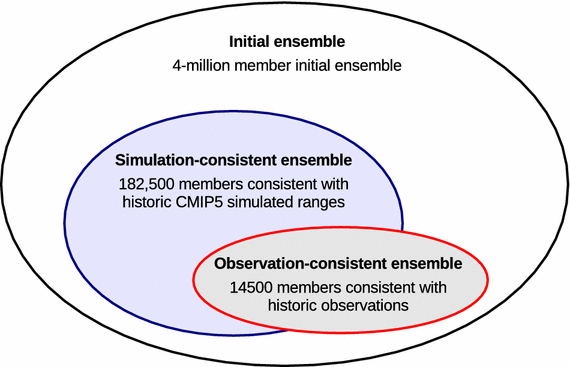
Hierarchy of the ensembles from the WASP model. The initial model ensemble contains 4-million members where two radiative forcing coefficients are varied with random-normal distributions to approximate uncertainty in historic radiative forcing (Fig. 3, black) and 14 input parameters are randomly varied between prescribed limits (Fig. 4, black). Of this initial model-ensemble, a Simulation–consistent ensemble is extracted comprising the 182,500 members that are consistent with 8 constraints based on the historic simulated ranges of the CMIP5 ensemble (Table 1). A further Observation–consistent ensemble is extracted comprising 14,500 members that are consistent with 8 historic observational constraints (Table 2). Some 8200 ensemble members are contained in both the historic Simulation–consistent and Observation–consistent ensembles
5.

The heat content change of the whole ocean from 1971 to 2005 is between 80 and 380 ZJ in the CMIP5 ensemble members analysed by (Flato et al. 2013);
6.

The heat added to the upper 700 m of the ocean from 1971 to 2005 is between 25 and 370 ZJ in the CMIP5 ensemble members analysed by (Flato et al. 2013). The upper ocean heat content is represented in WASP by the sum of the mixed layer and upper ocean boxes (Fig. 2; see Appendix Table 5).
7.

The residual terrestrial carbon uptake from 1986 to 2005 is between 0 and 3.0 PgC yr⁻¹ in the CMIP5 models analysed by (Flato et al. 2013).
8.

The ocean carbon uptake from 1986 to 2005 is between 1.6 and 2.3 PgC yr⁻¹ in the CMIP5 models analysed by (Flato et al. 2013).

To be counted as historically consistent with the CMIP5 ensemble, a WASP ensemble-member must lie within all eight of these ranges. Of the 4-million initial Monte Carlo WASP ensemble members, some 182,500 are judged to be simulation–consistent with the historical range of the CMIP5 ensemble (Figs. 3, 4, blue). These 182,500 ensemble members make up the simulation–consistent model ensemble (Fig. 5). There are small variations in number of simulation–consistent ensemble members for each RCP scenario, reflecting small differences in prescribed forcing between 2005 and 2012 (Meinshausen et al. 2011).

The simulation–consistent ESM-ensemble is able to reproduce the majority of CMIP5 historical simulation–range parameter space (Table 2) with two exceptions. Firstly, there are slightly reduced ranges in simulated warming relative to the 1961–1990 average, with the efficient ESM unable to reproduce the lowest warming from 1850 or the greatest warming up to 2005 (Table 1). This may reflect the lack of internal variability in the efficient ESM, since the CMIP5-simulated warming ranges reflect both an anthropogenic signal and internal variability but the efficient ESM ensemble reflects only the anthropogenic signal. Secondly, there is a reduced range of simulated ocean heat uptake by the upper 700 m of the ocean from 1971 to 2005 (Table 1), although the entire range of CMIP5-simulated total ocean heat uptake for this period is represented in the efficient ESM ensemble. The reduced range of simulated heat uptake for the upper 700 m of the ocean is likely to be the result of the simplistic box-model representation of the ocean regions in WASP (Fig. 2), relative to the 3D spatial representation of ocean regions in the CMIP5 models.

Table 2

The observational constraints used to assess for observation–consistency and the resulting ranges in the observation–consistent model-ensemble

Climate system property	Observation constraint (90 % range)	Observation–consistent model ensemble (5th–95th percentile)	Simulation–consistent model ensemble (5th–95th percentile)
Warming from 1850–1900 to 1993–2012	0.72–0.85 K	0.71–0.86 K	0.71–1.46 K
Decadal warming rate from 1951 to 2012	0.09–0.14 K decade⁻¹	0.09–0.11 K decade⁻¹	0.09–0.19 K decade⁻¹
Decadal SST warming from 1971 to 2010	0.09–0.13 K decade⁻¹	0.08–0.13 K decade⁻¹	0.04–0.12 K decade⁻¹
Earth System heat content increase from 1971 to 2010	196–351 ZJ	232–366 ZJ	122–470 ZJ
Earth System heat content increase from 1993 to 2010	127–201 ZJ	116–186 ZJ	60–240 ZJ
Upper 700 m ocean heat content increase from 1971 to 2010	82–154 TW	92–140 TW	54–160 TW
Cumulative ocean carbon uptake	125–185 PgC	124–173 PgC	118–157 PgC
Cumulative terrestrial carbon uptake	70–250 PgC	56–263 PgC	10–208 PgC

Also shown are the ranges for the simulation–consistent ensemble

2.4 Extracting the observationally consistent model ensemble

At year 2012, the initial 4-million ensemble-members are checked against eight observational constraints reflecting anthropogenic surface warming, heat uptake and carbon uptake (Table 2).

The eight separate observational constraints used to assess the ensemble members for observation-consistency (Table 2) are again chosen to cover the climate variables that the efficient ESM can simulate: global mean surface warming, ocean heat uptake and ocean and terrestrial carbon uptake (Fig. 2). However, these constraints represent metrics used to express the historic observations of climate change in the literature (e.g. Ciais et al. 2013; Hartmann et al. 2013; Rhein et al. 2013). The eight historic constraints are:

1.

Global mean Surface Air Temperature (SAT) warming from the 1850–1900 to the 2003–2012 periods is from 0.72 to 0.85 K (Hartmann et al. 2013);
2.

The mean decadal rate of SAT warming from 1951 to 2012 is from 0.09 to 0.14 K decade⁻¹ (Hartmann et al. 2013);
3.

The decadal Sea Surface Temperature (SST) warming rate from 1971 to 2010 is from 0.09 to 0.13 K decade⁻¹ (Rhein et al. 2013; as represented in WASP by the mixed layer ocean box, Fig. 2);
4.

The heat content change of the Earth System from 1971 to 2010 is from 196 to 351 ZJ (Rhein et al. 2013);
5.

The heat content change of the Earth System from 1993 to 2010 is from 127 to 201 ZJ (Rhein et al. 2013);
6.

The heat added to the upper 700 m of the ocean from 1971 to 2010 is from 82 to 154 TW (Rhein et al. 2013; as represented in WASP by the sum of the mixed layer and upper ocean boxes, Fig. 2; see Appendix Table 5),
7.

The residual terrestrial anthropogenic carbon uptake since the preindustrial is from 70 to 250 PgC (Ciais et al. 2013); and
8.

The anthropogenic ocean carbon uptake since the preindustrial is from 125 to 185 PgC (Ciais et al. 2013).

These eight observational constraints represent the estimated 90 % ranges for each quantity (Table 2). Each WASP ensemble member is therefore judged to be observation–consistent if it lies within the estimated 90 % range (Table 2) of at least 7 of the 8 observational constraints, and may miss the 90 % range of the remaining constraint by up to an extra 50 % relative to the best estimate. Allowing an ensemble-member to be classified as observation–consistent while missing the 90 % range for one out of eight observation–constraints provides a mechanism for the tails of the distribution for each observational constraint to be included in the observation–consistent model ensemble.

Of the 4-million initial ensemble members (Figs. 3, 4, black), those judged to be observationally-consistent are extracted to form an observationally-consistent model-ensemble of some 14,500 members (Figs. 3, 4, red; Fig. 5).

The observation–consistent ESM-ensemble is able to reproduce the majority of observational–consistent parameter space (Table 2) with two exceptions. Firstly, the observation–constrained ESM-ensemble shows a reduced range for the decadal rate of SAT warming from 1951 to 2012. This reduced range is interpreted here as a result of the simple ESM having no internal decadal temperature variability, which reduces the possible range of temperature change achieved by the simple ESM between two specific years and over short periods of time. Secondly, the simulated Earth System heat content increase shows reduced ranges, missing the lower end of the observational range for the 1971–2010 period but missing the upper end of the observational range for the 1993–2010 period. It is unclear precisely why this discrepancy arises, though it may result from the simplicity of ocean circulation and heat uptake representations in WASP, comprising of a surface mixed layer ocean attached to four sub-surface ocean regions with fixed e-folding tracer equilibration timescales (Fig. 2).

3 Model ensemble results and projections

3.1 Twenty-first century warming projections

For each RCP scenario, the twenty-first century warming projection ranges for the simulation–consistent efficient ESM-ensemble (Fig. 5; Table 1) are similar to the ranges from the CMIP5 ensemble of complex climate models (Fig. 1, compare WASP (simulation–consistent) to CMIP5, and Table 3, compare to IPCC 2013; tables SPM.2 and SPM.3 therein). This suggests that the WASP climate model represents a viable tool to quickly emulate future global mean warming ranges simulated an ensemble of complex climate models, given their historic performance to anthropogenic forcing. The WASP observation–consistent ensemble (Fig. 5; Table 2) can be considered in this way: an emulation of the projected warming ranges that may be simulated by a complex climate model ensemble, if the historic ranges of the complex climate model ensemble closely matched historic observations (Table 2).

Table 3

Twenty-first century warming projections from the observation–consistent and simulation–consistent WASP model ensembles for the four RCP scenarios

	Warming from 1986–2005 to 2086–2100 (K)
	Observation–consistent ensemble		Simulation–consistent ensemble
	Mean (K)	5th–95th percentile (K)	Mean (K)	5th–95th percentile (K)
RCP2.6	0.8	0.5–1.4	0.9	0.5–1.7
RCP4.5	1.4	1.0–2.0	1.6	1.0–2.6
RCP6.0	1.7	1.3–2.2	2.0	1.4–3.1
RCP8.5	2.5	2.2–3.0	3.0	2.2–4.6

Now consider the twenty-first century warming projections made by the observation–consistent ensemble (Fig. 1a). The observation–consistent ensemble has narrower ranges for future projected warming than the simulation–consistent ensemble (Fig. 1a), reflecting the narrower historical performance range of the observation–consistent ensemble (Table 2, compare observation–consistent to simulation–consistent ensembles). For each RCP scenario, the lower bounds of the projected warming range agree with the CMIP5 ensemble (Fig. 1a, compare WASP (observation–consistent) to CMIP5, and Table 3, compare to IPCC 2013; tables SPM.2 and SPM.3 therein). However, the projected upper bounds for twenty-first century warming are significantly reduced compared to CMIP5 for all RCP scenarios (Fig. 1a). Thus, the upper components of the projected warming ranges made by the simulation–consistent ensemble are not supported by historic observations [Fig. 1a, compare WASP (simulation–consistent) with WASP (observation–consistent)]. The close agreement between the simulation–consistent ensemble and CMIP5 also suggests that further work is required to establish whether the upper bounds of the CMIP5 projections are also not supported by observations (Fig. 1a).

3.2 Twenty-first century compatible carbon emission projections

Projected compatible carbon emission ranges in both the simulation–consistent and observation–consistent ensembles overlap with, but are generally greater than, the CMIP5 ranges (Fig. 1b), and are most similar for RCPs 3PD and 4.5 scenarios. However, the size of the ranges themselves (i.e. the 95th percentile minus the 5th percentile) are similar across all model ensembles. These similar sized ranges suggest that the variation in compatible carbon emissions between CMIP5 models encapsulates, but does not exceed, the uncertainty implied by carbon cycle observations.

The greater compatible carbon emissions projections made by the efficient ESM compared to CMIP5 models, especially for RCPs 6.0 and 8.5 (Fig. 1b), may be the result of the relatively simple representation of the carbon cycle in WASP (Fig. 2; “Appendix” section). For example, the hydrological cycle is not represented in WASP, but may significantly influence the response of the carbon cycle to emissions (e.g. Alexandrov et al. 2003). Also, there are likely to be regional differences in the responses of the carbon cycle to warming and rising CO₂ (e.g. Alexandrov et al. 2003), and such regional differences are not represented in WASP (Fig. 2; “Appendix” section).

3.3 Climate system parameters

The sensitivity of climate to carbon emissions is often characterised by the Equilibrium Climate Sensitivity (ECS, in K) and the Transient Climate Response to Emission [TCRE, in K (1000 PgC)⁻¹] (IPCC 2013).

The Equilibrium Climate Sensitivity represents the equilibrium surface warming for a sustained doubling of atmospheric CO₂, and is calculated for the WASP ensemble members by $ {\text{ECS}} = a_{{{\text{CO}}_{2} }} \ln 2/\lambda $. The random-normal input distribution for $ a_{{{\text{CO}}_{2} }} $ (Fig. 3a, black) reflects current uncertainty in the CO₂-radiative forcing link (Myhre et al. 2013), while the random-linear input distribution for λ (Fig. 4a, black) assumes λ must lie between 0.1 and 5.0 Wm⁻² K⁻¹, but no prior knowledge of relative weighting to particular values within this range is assumed. These input distributions result in the ECS ranging from a minimum of 0.6 K to a maximum of 43 K in the initial 4-million member ensemble.

Now consider how the constraints used to select the simulation–consistent ensemble (Table 1) and observation–consistent ensemble (Table 2) restricts this broad range of ECS values. The 14 500 observation–consistent ensemble members have mean ECS of 2.4 K and a 5th to 95th percentile range of 1.4–4.4 K (Fig. 4b, red), almost identical to the IPCC best estimate range of 1.5–4.5 K (Bindoff et al. 2013). The IPCC best estimate for the ECS is in part based on the same observational constraints (Table 2) and historic forcing estimates (Fig. 3, black; Myhre et al. 2013) used to constrain the observation–consistent model ensemble, and so these two ECS ranges are not independent of one another. However, their close agreement does provide confidence that the WASP model framework is a viable and efficient tool to use observations of the climate system to constrain climate parameters.

For the 182,500 simulation–consistent ensemble-members, the mean ECS is 2.9 K while the 5th to 95th percentile range is 1.4–5.6 K (Fig. 4b, blue). This mean value is comparable to the mean for the CMIP5 ensemble members of 3.2 K (Flato et al. 2013). However, the ECS range is greater the CMIP5 ensemble range of 2.1–4.7 K (Flato et al. 2013). The greater ECS range in the simulation–consistent ensemble may reflect the far greater number of ensemble-members, covering a greater extent of parameter space. While the historic performance of the simulation–consistent ensemble matches the range simulated by CMIP5 (Table 1), there are more different ways of achieving this historic performance range explored in the simulation–consistent ensemble due to the much greater number of ensemble-members.

The Transient Climate Response to Emission (TCRE) represents the anthropogenic surface warming per unit cumulative carbon emitted since the preindustrial period at a specified point in time. The 5th–95th percentile range for the TCRE, evaluated at year 2100 for RCP8.5, is 1.1–2.7 K (1000 PgC)⁻¹ for the simulation–consistent ensemble and 1.0–1.6 K (1000 PgC)⁻¹ for the observation–consistent ensemble. These ranges are consistent with the IPCC best estimate of between 0.8 and 2.5 K (1000 PgC)⁻¹ for the late twenty-first century (IPCC 2013), although the observation–consistent ensemble range is narrower and concentrated towards the lower end of the IPCC estimate.

The observation–consistent and simulation–consistent ensemble ranges for the equilibrium warming ratios r _SST:SAT (Fig. 3d) and r _sub:SST (Fig. 3e) encompass values consistent with the ranges of these ratios in more complex 3D models following idealised carbon emissions previously analysed by Williams et al. (2012; see Fig. 3 therein). Other properties, such as the efficacy of ocean heat uptake (Fig. 3c), fraction of total Earth system heat uptake by the ocean (Fig. 3f), and other parameters (Fig. 3h–o) have similar frequency distributions for observation–consistent and simulation–consistent (Fig. 3, red and blue) to the input distribution (Fig. 3, black), implying that these properties are not well constrained by the historical tests used (Tables 1, 2).

4 Discussion

A new Earth System Model was presented for efficient projection of the global mean impacts of carbon emissions: the Warming Acidification and Sea-level Projector (WASP: Fig. 2; “Appendix” section). This new model was then used to construct an initial 4-million member Monte Carlo ensemble with randomly varied parameter values (Figs. 3, 4, black), which were forced with historic CO₂ concentrations and future RCP scenarios to year 2100 (Meinshausen et al. 2011).

Eight historic constraints, representing the historic warming, heat and carbon ranges simulated by the CMIP5 ensemble (Table 1), were used to extract a simulation–consistent model ensemble of 182,500 members (Fig. 5; Figs. 3, 4, blue). This simulation–consistent model ensemble was then used to make projections of future warming and compatible carbon emissions for four RCP scenarios (Fig. 1; Tables 3, 4). These projections are in good agreement with the projection ranges from the complex CMIP5 model ensemble (Fig. 1, and compare Tables 3, 4 to IPCC, 2013; tables SPM.2 and SPM.3 therein). It should be noted, however, that the WASP model does not contain internal climate variability, but the CMIP5 models do. This lack of internal climate variability in WASP constitutes an important caveat when comparing both the historic performance and future projections of CMIP5 to the simulation–consistent model ensemble.

Table 4

Twenty-first century compatible carbon emission projections from the observation–consistent and simulation–consistent WASP model ensembles for the four RCP scenarios

	Compatible cumulative carbon emission 2012–2100 (PgC)
	Observation–consistent ensemble		Simulation–consistent ensemble
	Mean (PgC)	5th–95th percentile (PgC)	Mean (PgC)	5th–95th percentile (PgC)
RCP2.6	360	240–480	310	180–430
RCP4.5	870	680–1060	770	590–960
RCP6.0	1310	1090–1550	1190	970–1410
RCP8.5	2220	1900–2570	2030	1720–2360

Starting again from the initial 4-million member ensemble, another eight constraints, this time representing observational ranges for historic warming, heat and carbon (Table 2), were used to extract an observation–consistent model ensemble of 14,500 members (Fig. 5; Figs. 3, 4, red). This observation–consistent model ensemble was then used to make twenty-first century projections of warming and compatible carbon emissions for the four RCP scenarios (Fig. 1; Tables 3, 4). The lower bounds of the projected twenty-first century warming for the observation–consistent ensemble are consistent with both the CMIP5 and simulation–consistent ranges for each RCP scenario (Fig. 1a). However, the upper bounds of projected warming are reduced by 20–35 %. This reduction shows that the upper bounds of projected warming in the simulation–consistent ensemble are not supported by historic observations.

Only 4.5 % of the 182,500 simulation–consistent ensemble members are also consistent with observations (Fig. 5). This implies that a large part of parameter space consistent with historic CMIP5 performance (Table 1) is not observation–consistent. Some 43 % of the 14,500 observation–consistent ensemble members (Fig. 5) lie outside the simulation–consistent ensemble (Table 1). Therefore, significant areas of observation–consistent parameter space are not currently contained within the historic CMIP5 performance-range.

The Equilibrium Climate Sensitivity range in the observation–consistent ensemble, of 1.4–4.4 K, is comparable to the IPCC estimate of 1.5–4.5 K (Bindoff et al. 2013). Also, the ranges of the Transient Climate Response to Emissions, TCRE, in the observation–consistent and simulation–consistent model ensembles are comparable to previous estimates based on models and (Collins et al. 2013; Gillet et al. 2013; Matthews et al. 2009; Zickfield et al. 2009, 2012) and observationally constrained theory (Goodwin et al. 2015). These agreements for the ECS, TCRE and projected warming ranges imply that the WASP model presented here (Fig. 2; “Appendix” section) is a useful tool, within a model-hierarchy, for quickly constraining climate parameter estimates and making future projections based on historic observations and historic model performance.

The possible impact on future climate projections of small discrepancies between the range of historic climate change simulated by models and observed in the real climate system is discussed in Assessment Report 5 (Flato et al. 2013) and elsewhere (e.g. England et al. 2013; Song et al. 2014). Dangerous climate change often refers to 2 K or more global mean surface warming above preindustrial, although other climate targets should also be considered (Steinacher et al. 2013). This equates to around an additional 1.4 K above the warming already achieved during the 1985–2005 period (IPCC 2013). This dangerous climate change limit is at the lower bounds of twenty-first century projections for RCP4.5 and RCP6.0 (Fig. 1; Collins et al. 2013), and is considerably below the lower bound of warming projected for RCP8.5. Here, close agreement is found for the lower bounds of twenty-first century warming projected by the CMIP5 ensemble and the observation–consistent ensemble (Fig. 1). This lower bound agreement implies that the projected likelihood of crossing the defined threshold for dangerous climate change is not significantly affected by small CMIP5-observation discrepancies in the historic period. Indeed, the observation–consistent ensemble presented here is in agreement with the CMIP5 ensemble in suggesting that, to stand a good chance of avoiding dangerous climate change by the end of the century, global emissions should be controlled to follow a path below RCP4.5, for example towards RCP3PD emission levels (Fig. 1).

Notes

Acknowledgments

This research was funded by the UK Natural Environment Research Council grant number NE/K012789/1.

Appendix: WASP model equations

Description of the efficient earth system model

This Appendix describes the equations used in the new efficient Earth System Model; the Warming, Acidification and Sea-level Projector (WASP) (Fig. 2).

Anthropogenic ocean heat uptake in the WASP model

WASP assumes that for an imposed radiative forcing, R _TOTAL (Wm⁻²), the eventual anthropogenic heat content increase for the ocean surface mixed layer at equilibrium, $ H_{equil}^{mixed} $ (J), is given via,

$$ {{H_{equil}^{mixed} } \mathord{\left/ {\vphantom {{H_{equil}^{mixed} } {V_{mixed} }}} \right. \kern-0pt} {V_{mixed} }} = c_{p} r_{SST:SAT} \lambda^{ - 1} R_{TOTAL} , $$

(3)

where r _SST:SAT is the ratio of warming for global SSTs and surface atmosphere temperatures at equilibrium, c _p is the mean specific heat capacity of seawater in the global ocean (Williams et al. 2012), and V _mixed is the volume of the surface mixed layer (Fig. 2). To calculate the rate of anthropogenic heat uptake by the Earth System in WASP, N (W m⁻²), the radiative forcing, R _TOTAL, is modulated by the fractional distance from the eventual anthropogenic heat uptake at equilibrium in the surface mixed layer at time t,

$$ N(t) = \left( {\frac{{H_{equil}^{mixed} (t) - H^{mixed} (t)}}{{H_{equil}^{mixed} (t)}}} \right)R_{TOTAL} (t), $$

(4)

where N for the whole Earth System is calculated by the distance from equilibrium heat uptake of the surface mixed layer. Equation (4) results in N(t) = R _TOTAL(t) initially, at the moment that R _TOTAL(t) is introduced and before the heat content of the mixed layer is increased, and N(t) = 0 at surface-ocean thermal equilibrium, once $ H^{mixed} = H_{equil}^{mixed} $. The anthropogenic heat uptake by ocean between times t − δt and t, δH (J), is given by,

$$ \delta H = f_{heat} A_{Earth} N\delta t, $$

(5)

where A _Earth is the surface area of the entire planet Earth (see Appendix Table 5), and f _heat is the fraction of whole Earth-System heat uptake within the ocean (Fig. 3f).

Table 5

Definitions of the fixed model parameters in WASP, and their values used in the model ensembles

WASP parameter description	Symbol	Standard value
Volume of ocean	V _total	1.3 × 10¹⁸ m³
Volume fraction of surface mixed layer	V _mixed /V _total	0.03
Volume fraction of upper water	V _upper /V _total	0.16
Volume fraction of intermediate water	V _inter /V _total	0.2
Volume fraction of deep water	V _deep /V _total	0.21
Volume fraction of bottom water	V _bottom /V _total	0.40
Surface area of planet	A _total	5.1 × 10¹⁴ m²
Surface area of ocean	A _ocean	3.5 × 10¹⁴m²
Global mean heat capacity of seawater	c _p	3910 J K⁻¹ kg⁻¹
Preindustrial Net Primary Productivity (NPP)	NPP ₀	60 PgC yr⁻¹
Preindustrial vegetation carbon	I _veg,0	450 PgC
Preindustrial soil carbon	I _soil,0	1500 PgC
Timestep	δt	0.1 years

The flux of anthropogenic heat content from the surface mixed layer into each sub-surface region between time t − δt and t, $ F_{Heat}^{mix \to region} $ (J), is calculated assuming that a passive tracer in the sub-surface ocean restores towards the mixed layer concentration according to defined e-folding timescales,

$$ \begin{aligned} F_{Heat}^{mix \to region} &= \left[ {H_{Usat}^{region} - r_{sub:SST} H_{Usat}^{mix} \left( {\frac{{V_{region} }}{{V_{mix} }}} \right)} \right]\exp \left( { - {{\delta t} \mathord{\left/ {\vphantom {{\delta t} {\tau_{region} }}} \right. \kern-0pt} {\tau_{region} }}} \right) \\ & \quad - \left[ {H_{Usat}^{region} - r_{sub:SST} H_{Usat}^{mix} \left( {\frac{{V_{region} }}{{V_{mix} }}} \right)} \right] \\ \end{aligned} $$

(6)

where τ _region (yr) refers to the restoring timescale for tracers to equilibrate in a sub-surface ocean region of volume V _region (m³) (where region refers to either the upper ocean, intermediate ocean, deep ocean or bottom ocean boxes, Fig. 2), H _region is the anthropogenic heat content of a sub-surface ocean region, V _mix (m³) is the volume of the surface mixed layer (see Appendix Table 5) and r _sub:SST is the ratio of warming for the global sub-surface ocean to global SSTs at equilibrium.

The change in anthropogenic heat content in the surface mixed layer between time t − δt and t, δH ^mixed (J), is then calculated from Eqs. (5) and (6), by,

$$ \delta H^{mixed} = A_{Earth} N(t)\delta t - F_{heat}^{mix \to upper} - F_{heat}^{mix \to inter} - F_{heat}^{mix \to deep} - F_{heat}^{mix \to bottom} , $$

(7)

while the changes in anthropogenic heat content in each sub-surface region, δH ^region (J), is given by,

$$ \delta H^{region} = F_{heat}^{mix \to region} . $$

(8)

The ocean carbon cycle in the WASP model

The WASP model code considers separately the cumulative carbon emission that has remained in the air–sea system since the preindustrial at time t, $ I_{em}^{At + Oc} (t) $ (PgC), and the residual carbon uptake by the terrestrial system since the preindustrial, ΔI _ter(t) (PgC), combining them together to find to total cumulative carbon emission, $ I_{em}^{TOTAL} (t), $

$$ I_{em}^{TOTAL} (t) = I_{em}^{At + Oc} (t) +\Delta I_{ter} (t), $$

(9)

where details of how ΔI _ter is calculated are given below in a later section of the Appendix.

In the timestep between times t − δt and t, CO₂ is emitted into the air–sea system, $ \delta I_{em}^{At + Oc} $ (PgC), and is assumed to enter the atmosphere, increasing the undersaturation of carbon in the ocean (Goodwin et al. 2015) by δI _Usat(emissions) (PgC). The increase in δI _Usat(emissions) from $ \delta I_{em}^{At + Oc} (t) $ is calculated by re-arranging the time-dependent CO₂ equation of Goodwin et al. (2015), $ \Delta \ln {\text{CO}}_{2} (t) = \left[ {I_{em}^{At + Oc} (t) + I_{Usat} (t)} \right]/I_{B} , $ and including an additional term for equivalent carbon emissions from the ocean temperature-CO₂ solubility feedback (Goodwin and Lenton 2009). Applying to a single time-step gives,

$$ \delta I_{Usat} (emissions) = I_{B} \ln \left( {\frac{{I_{CO2} + \delta I_{em}^{At + Oc} + \delta I_{em}^{heat} }}{{I_{CO2} }}} \right) - \left( {\delta I_{em}^{At + Oc} + \delta I_{em}^{heat} } \right), $$

(10)

where $ I_{{{\text{CO}}_{2} }} $ is the amount of CO₂ in the atmosphere in PgC, I _B (PgC) is the buffered carbon inventory (Goodwin et al. 2007), and $ \delta I_{em}^{heat} $(PgC) is the additional term representing the equivalent carbon emission from the temperature-solubility feedback between times t − δt and t. $ \delta I_{em}^{heat} $ is calculated using the methodology of Goodwin and Lenton (2009) using

$$ \delta I_{em}^{heat} = - \left( {\frac{{\partial C_{sat} }}{\partial T}} \right)\frac{{\delta H^{mix} }}{{c_{p} }}, $$

(11)

where ∂C _sat/∂T is the sensitivity of DIC solubility to temperature, given in WASP by $ {{\partial C_{sat} } \mathord{\left/ {\vphantom {{\partial C_{sat} } {\partial T}}} \right. \kern-0pt} {\partial T}} = - 0.1 + 0.025\;\Delta \ln {\text{CO}}_{2} $ in g C m⁻³ K⁻¹ (Goodwin and Lenton 2009; see Fig. 2 therein). The total $ \delta I_{Usat} (emissions) $ for the whole ocean (Eq. 10) is apportioned to the different ocean boxes (Fig. 2) according to their volume by,

$$ \delta I_{Usat}^{region} (emissions) = \left( {\frac{{V^{region} }}{{V^{total} }}} \right)\left[ {I_{B} \ln \left( {\frac{{I_{{{\text{CO}}_{2} }} + \delta I_{em}^{At + Oc} + \delta I_{em}^{heat} }}{{I_{{{\text{CO}}_{2} }} }}} \right) - \left( {\delta I_{em}^{At + Oc} + \delta I_{em}^{heat} } \right)} \right]. $$

(12)

The flux of carbon from the atmosphere to the surface mixed layer between times t − δt and t, $ F_{Usat}^{air \to mix} $ (PgC), acts to reduce mixed-layer I _Usat over an e-folding timescale $ \tau_{mix} $(yr), via,

$$ F_{Usat}^{air \to mix} = I_{Usat}^{mixed} (t - \delta t)\left( {1 - \exp \left( {\frac{ - \delta t}{{\tau_{mix} }}} \right)} \right). $$

(13)

The flux of I _Usat exchanged from the mixed layer to each sub-surface ocean region between times t − δt and t, $ F_{Usat}^{mix \to region} $ (PgC), is calculated using the same restoring timescales as for the heat content fluxes, analogous to Eq. (6), via,

$$ F_{Usat}^{mix \to region} = \left[ {I_{Usat}^{region} - I_{Usat}^{mix} \left( {{{V^{region} } \mathord{\left/ {\vphantom {{V^{region} } {V^{mix} }}} \right. \kern-0pt} {V^{mix} }}} \right)} \right]\exp \left( { - {{\delta t} \mathord{\left/ {\vphantom {{\delta t} {\tau^{region} }}} \right. \kern-0pt} {\tau^{region} }}} \right) - \left[ {I_{Usat}^{region} - I_{Usat}^{mix} \left( {{{V^{region} } \mathord{\left/ {\vphantom {{V^{region} } {V^{mix} }}} \right. \kern-0pt} {V^{mix} }}} \right)} \right]. $$

(14)

Therefore, the overall change in I _Usat in the mixed layer between t − δt and t, $ \delta I_{Usat}^{mix} $ (PgC), is given by,

$$ \delta I_{Usat}^{mix} = \delta I_{Usat}^{mix} (emissions) + F_{Usat}^{air \to mix} - F_{Usat}^{mix \to upper} - F_{Usat}^{mix \to inter} - F_{Usat}^{mix \to deep} - F_{Usat}^{mix \to bottom} , $$

(15)

while the changes in the sub-surface regions, $ \delta I_{Usat}^{region} $ (PgC), are given by,

$$ \delta I_{Usat}^{region} = \delta I_{Usat}^{region} (emissions) + F_{Usat}^{mix \to region} . $$

(16)

The sum of all changes to undersaturation carbon content in all timesteps since the preindustrial, and for all ocean regions, is then used to calculate the total cumulative ocean carbon undersaturation at time t, I _Usat(t) (PgC), via,

$$ I_{Usat} (t) = I_{Usat}^{mix} (t) + I_{Usat}^{upper} (t) + I_{Usat}^{{\text{int} er}} (t) + I_{Usat}^{deep} (t) + I_{Usat}^{bottom} (t). $$

(17)

Atmospheric CO₂ at time t, CO₂ (ppm), is then calculated using the time-dependent CO₂ relationship of Goodwin et al. (2015), with the additional term representing equivalent carbon emissions from the ocean temperature-CO₂ solubility feedback,

$$ {\text{CO}}_{2} (t) = {\text{CO}}_{2} (t_{0} )\exp \left( {\frac{{I_{em}^{At + Oc} (t) + I_{Usat}^{total} (t) + I_{em}^{heat} (t)}}{{I_{B} }}} \right), $$

(18)

where t ₀ refers to the preindustrial.

Sea-surface ocean acidification in WASP is calculated by using coefficients for the sensitivity of pH to Δln CO₂ for seawater at chemical saturation with overlying atmospheric CO₂, and for the sensitivity of pH to the distance of DIC from CO₂ saturation in the mixed layer. This results in,

$$ \Delta pH(t) = c_{pH1}\Delta \ln {\text{CO}}_{2} (t) + c_{pH2} \left( {{{ - I_{Usat}^{mix} } \mathord{\left/ {\vphantom {{ - I_{Usat}^{mix} } {V^{mix} }}} \right. \kern-0pt} {V^{mix} }}} \right), $$

(19)

where the values c _pH1 and c _pH2 are calculated from perturbation experiments using an explicit numerical carbonate chemistry solver (Follows et al. 2006).

When carbon emissions are set to restore CO₂ to a prescribed pathway, CO ₂ ^restore (t) (Meinshausen et al. 2011), the carbon emissions added into the air–sea system between times t − δt and t, $ \delta I_{em}^{At + Oc} $, are set equal to the flux of undersaturation carbon from the air to the mixed layer flux from t − δt to t, plus 0.9 times the difference between the prescribes CO₂ mixing ratio being restored towards at time t, and the actual model CO₂ mixing ratio at t − δt,

$$ \delta I_{em}^{At + Oc} = F_{Usat}^{mix} + 0.9 \times \left( {{\text{CO}}_{2}^{restore} (t) - {\text{CO}}_{2} (t - \delta t)} \right), $$

(20)

where the factor of 0.9 is used to prevent CO₂ from overshooting the restored value and causing a numerical instability whereby the simulated CO₂ value oscillates around the prescribed pathway.

Anthropogenic surface warming in the WASP model

In WASP, the warming-CO₂ emission relationship of Goodwin et al. (2015) is applied to calculate global mean surface warming, with additional terms for the radiative forcing from both Kyoto-protocol agents other than CO₂, $ R_{{non{-}{\text{CO}}_{2} }} $ (W m⁻²), and from non-Kyoto agents, R _non-Kyoto (Wm⁻²), and an additional term representing the equivalent cumulative carbon emissions from the ocean temperature-CO₂ solubility feedback, $ I_{em}^{heat} $(PgC) (Goodwin and Lenton 2009). The anthropogenic warming at time t, ΔT (K), is calculated via,

$$ \Delta T(t) = \left( {\frac{1}{\lambda }} \right)\left( {1 - \frac{\varepsilon N(t)}{R(t)}} \right)\left\{ {\left[ {\left( {\frac{a}{{I_{B} }}} \right)\left( {I_{Usat} (t) + I_{em}^{At + Oc} (t) + I_{em}^{heat} (t)} \right)} \right] + R_{{non{-}{\text{CO}}_{2} }} (t) + R_{non{-}Kyoto} (t)} \right\}. $$

(21)

where ε is the efficacy of ocean heat uptake, a = 5.35 Wm⁻² is the radiative forcing coefficient from a log change in CO₂ (Myhre et al. 1998), and $ R_{{non{-}{\text{CO}}_{2} }} $ is an input parameter from the RCP scenario definitions (Meinshausen et al. 2011), and R _non-Kyoto is scaled from $ R_{{non{-}{\text{CO}}_{2} }} $ after Eq. (2) to capture uncertainty in anthropogenic radiative forcing.

WASP can also simulate the thermosteric and isostatic contributions to global mean sea level rise using the internally simulated ocean heat uptake and surface warming. The thermosteric contribution to sea level rise can be estimated as a function of ocean heat uptake after Williams et al. (2012; see Eq. 4 therein), while the semi-empirical approach of Rahmstorf (2007) can be applied for isostatic sea level rise (Rahmstorf 2007; see Eq. 1 therein).

Terrestrial carbon cycling in the WASP model

Terrestrial carbon is represented by soil carbon and vegetation carbon reservoirs (Fig. 2). The rates of change of vegetation carbon, I _veg (PgC) and soil carbon, I _soil (PgC), reservoirs at time t are modelled by,

$$ \frac{{dI_{Veg} }}{dt}(t) = {\text{NPP}}(t_{0} )f_{1} (\Delta T)f_{2} ({\text{CO}}_{2} ) - LL(t_{0} )\frac{{I_{Veg} (t)}}{{I_{Veg} (t_{0} )}}, $$

(22)

and,

$$ \frac{{dI_{Soil} }}{dt}(t) = {\text{LL}}(t_{0} )\frac{{I_{Veg} (t)}}{{I_{Veg} (t_{0} )}} - {\text{SR}}(t_{0} )\frac{{I_{Soil} (t)}}{{I_{Soil} (t_{0} )}}f_{3} (\Delta T), $$

(23)

where NPP (PgC yr⁻¹) is net primary production, LL (PgC yr⁻¹) is leaf litter fallout and SR (PgC yr⁻¹) is soil respiration (Fig. 2), and t ₀ refers to the preindustrial. At preindustrial steady state, t = t ₀ the system is in balance, giving,

$$ {\text{NPP}}(t_{0} ) = {\text{LL}}(t_{0} ) = {\text{SR}}(t_{0} ). $$

(24)

The functions f ₁–f ₃ must return unity at preindustrial CO₂ and ΔT = 0. A simple linear response of global NPP to global mean surface warming is assumed, hiding a multitude of mechanistic factors, giving,

$$ f_{1} (\Delta T) = 1 + \frac{{\left( {{{\partial {\text{NPP}}} \mathord{\left/ {\vphantom {{\partial {\text{NPP}}} {\partial T}}} \right. \kern-0pt} {\partial T}}} \right)}}{{{\text{NPP}}(t_{0} )}}\Delta T. $$

(25)

The response of global NPP to CO₂ is modelled by an empirical CO₂-fertilisation effect related to the log-change in atmospheric CO₂ (Alexandrov et al. 2003), resulting in a function f ₂ in (22) of,

$$ f_{2} ({\text{CO}}_{2} ) = 1.0 + \gamma_{{{\text{CO}}_{2} }}\Delta \ln {\text{CO}}_{2} , $$

(26)

where $ \gamma_{{{\text{CO}}_{2} }} $ is the Keeling-equation CO₂-fertilisation growth factor (Alexandrov et al. 2003). Global mean soil carbon residence time is assumed to be linearly related to warming, ΔT, via a specified sensitivity, ∂τ/∂T (yr K⁻¹), using,

$$ f_{3} (\Delta T) = \frac{{\tau (t_{0} )}}{\tau (t)} = \frac{{\left( {{{I_{Soil} (t_{0} )} \mathord{\left/ {\vphantom {{I_{Soil} (t_{0} )} {{\text{NPP}}(t_{0} )}}} \right. \kern-0pt} {{\text{NPP}}(t_{0} )}}} \right)}}{{\left( {{{I_{Soil} (t_{0} )} \mathord{\left/ {\vphantom {{I_{Soil} (t_{0} )} {{\text{NPP}}(t_{0} )}}} \right. \kern-0pt} {{\text{NPP}}(t_{0} )}}} \right) + \left( {{{\partial \tau } \mathord{\left/ {\vphantom {{\partial \tau } {\partial T}}} \right. \kern-0pt} {\partial T}}} \right)\Delta T}} $$

(27)

The cumulative changes in I _soil and I _veg over time since the preindustrial, ΔI _soil and ΔI _veg respectively, are calculated and summed to give the total change in terrestrial carbon since the preindustrial,

$$ \Delta I_{ter} =\Delta I_{soil} +\Delta I_{veg} , $$

(28)

and combined with the cumulative emission to the air–sea system, $ I_{em}^{At + Oc} $, to give the total compatible carbon emission using Eq. (9).

References

Alexandrov GA, Oikawa T, Yamagata Y (2003) Climate dependence of the CO₂ fertilization effect on terrestrial net primary production. Tellus 55B:669–675CrossRefGoogle Scholar
Bindoff NL, Stott PA, AchutaRao KM, Allen MR, Gillett N, Gutzler D, Hansingo K, Hegerl G, Hu Y, Jain S, Mokhov II, Overland J, Perlwitz J, Sebbari R, Zhang X (2013) Detection and attribution of climate change: from global to regional. In: Stocker TF, Qin D, Plattner G-K, Tignor M, Allen SK, Boschung J, Nauels A, Xia Y, Bex V, Midgley PM (eds) Climate change 2013: the physical science basis. Contribution of working group I to the fifth assessment report of the intergovernmental panel on climate change. Cambridge University Press, Cambridge, New York, NY, pp 867–952Google Scholar
Ciais P, Sabine C, Bala G, Bopp L, Brovkin V, Canadell J, Chhabra A, DeFries R, Galloway J, Heimann M, Jones C, Le Quéré C, Myneni RB, Piao S, Thornton P (2013) Carbon and other biogeochemical cycles. In: Stocker TF, Qin D, Plattner G-K, Tignor M, Allen SK, Boschung J, Nauels A, Xia Y, Bex V, Midgley PM (eds) Climate change 2013: the physical science basis. Contribution of working group I to the fifth assessment report of the intergovernmental panel on climate change. Cambridge University Press, Cambridge, New York, NY, pp 465–570Google Scholar
Collins M, Knutti R, Arblaster J, Dufresne J-L, Fichefet T, Friedlingstein P, Gao X, Gutowski WJ, Johns T, Krinner G, Shongwe M, Tebaldi C, Weaver AJ, Wehner M (2013) Long-term climate change: projections, commitments and irreversibility. In: Stocker TF, Qin D, Plattner G-K, Tignor M, Allen SK, Boschung J, Nauels A, Xia Y, Bex V, Midgley PM (eds) Climate change 2013: the physical science basis. Contribution of working group I to the fifth assessment report of the intergovernmental panel on climate change. Cambridge University Press, Cambridge, New York, NY, pp 1029–1136Google Scholar
DeVries T, Primeau F (2011) Dynamically and observationally constrained estimates of water-mass distributions and ages in the global ocean. J Phys Oceanogr 41:2381–2401. doi: 10.1175/JPO-D-10-05011.1 CrossRefGoogle Scholar
England MH, Kajtar JB, Maher N (2013) Robust warming projections despite the recent hiatus. Nat Clim Change 5:394–395CrossRefGoogle Scholar
Flato G, Marotzke J, Abiodun B, Braconnot P, Chou SC, Collins W, Cox P, Driouech F, Emori S, Eyring V, Forest C, Gleckler P, Guilyardi E, Jakob C, Kattsov V, Reason C, Rummukainen M (2013) Evaluation of climate models. In: Stocker TF, Qin D, Plattner G-K, Tignor M, Allen SK, Boschung J, Nauels A, Xia Y, Bex V, Midgley PM (eds) Climate change 2013: the physical science basis. Contribution of working group I to the fifth assessment report of the intergovernmental panel on climate change. Cambridge University Press, Cambridge, New York, NY, pp 741–866Google Scholar
Follows MJ, Dutkiewicz S, Ito T (2006) On the solution of the carbonate system in ocean biogeochemistry models. Ocean Model 12:290–301. doi: 10.1016/j.ocemod.2005.05.004 CrossRefGoogle Scholar
Friedlingstein P et al (2006) Climate-carbon cycle feedback analysis: result from the C4MIP model intercomparison. J Clim 19:3337–3353CrossRefGoogle Scholar
Frölicher TL, Winton M, Sarmiento JL (2014) Continued global warming after CO₂ emissions stoppage. Nat Clim Change 4:40–44CrossRefGoogle Scholar
Geoffroy O et al (2013) Transient climate response in a two-layer energy-balance model. Part II: representation of the efficacy of deep-ocean heat uptake and validation for CMIP5 AOGCMs. J Clim 26:1859–1876CrossRefGoogle Scholar
Gillet NP, Arora VK, Matthews D, Allen MR (2013) Constraining the ratio of global warming to cumulative CO₂ emissions using CMIP5 simulations. J Clim 26:6844–6858CrossRefGoogle Scholar
Goodwin P, Lenton TM (2009) Quantifying the feedback between ocean heating and CO₂ solubility as an equivalent carbon emission. Geophys Res Lett 36:L15609CrossRefGoogle Scholar
Goodwin P, Williams RG, Follows MJ, Dutkiewicz S (2007) Ocean-atmosphere partitioning of anthropogenic carbon dioxide on centennial timescales. Glob Biogeochem Cycles 21:GB1014CrossRefGoogle Scholar
Goodwin P, Williams RG, Ridgwell A, Follows MJ (2009) Climate sensitivity to the carbon cycle modulated by past and future changes to ocean chemistry. Nat Geosci 2:145–150CrossRefGoogle Scholar
Goodwin P, Williams RG, Ridgwell A (2015) Sensitivity of climate to cumulative carbon emissions due to compensation of ocean heat and carbon uptake. Nat Geosci 8:29–34CrossRefGoogle Scholar
Hartmann DL, Klein Tank AMG, Rusticucci M, Alexander LV, Brönnimann S, Charabi Y, Dentener FJ, Dlugokencky EJ, Easterling DR, Kaplan A, Soden BJ, Thorne PW, Wild M, Zhai PM (2013) Observations: atmosphere and surface. In: Stocker TF, Qin D, Plattner G-K, Tignor M, Allen SK, Boschung J, Nauels A, Xia Y, Bex V, Midgley PM (eds) Climate change 2013: the physical science basis. Contribution of working group I to the fifth assessment report of the intergovernmental panel on climate change. Cambridge University Press, Cambridge, New York, NY, pp 159–254Google Scholar
IPCC (2013) Summary for policy makers. In: Stocker TF, Qin D, Plattner G-K, Tignor M, Allen SK, Boschung J, Nauels A, Xia Y, Bex V, Midgley PM (eds) Climate change 2013: the physical science basis. Contribution of working group I to the fifth assessment report of the intergovernmental panel on climate change. IPCC, Cambridge University Press, Cambridge, New York, NYGoogle Scholar
Jha B, Hu Z-Z, Kunar A (2014) SST and ENSO variability and change simulated in historical experiments of CMIP5 models. Clim Dyn 42:2113–2124. doi: 10.1007/s00382-013-1803-z CrossRefGoogle Scholar
Matthews HD, Gillet NP, Stott PA, Zickfield K (2009) The proportionality of global warming to cumulative carbon emissions. Nature 459:829–832CrossRefGoogle Scholar
Meinshausen M et al (2011) The RCP greenhouse gas concentrations and their extensions from 1765 to 2300. Clim Change 109:213–241CrossRefGoogle Scholar
Myhre G, Highwood EJ, Shine KP, Stordal F (1998) New estimates of radiative forcing due to well mixed greenhouse gases. Geophys Res Lett 25:2715–2718CrossRefGoogle Scholar
Myhre G, Shindell D, Breon F-M, Collins W, Fuglestvedt J, Huang J, Koch D, Lamarque J-F, Lee D, Mendoza B, Nakajima T, Robock A, Stephens G, Takemura T, Zhang H (2013) Anthropogenic and natural radiative forcing. In: Stocker TF, Qin D, Plattner G-K, Tignor M, Allen SK, Boschung J, Nauels A, Xia Y, Bex V, Midgley PM (eds) Climate change 2013: the physical science basis. Contribution of working group I to the fifth assessment report of the intergovernmental panel on climate change. Cambridge University Press, Cambridge, New York, NY, pp 659–740Google Scholar
Pierrehumbert RT (2014) Short-lived climate pollution. Annu Rev Earth Planet Sci 42:341–379CrossRefGoogle Scholar
Rahmstorf S (2007) A semi-empirical approach to projecting future sea-level rise. Science 315:368–370CrossRefGoogle Scholar
Rhein M, Rintoul SR, Aoki S, Campos E, Chambers D, Feely RA, Gulev S, Johnson GC, Josey SA, Kostianoy A, Mauritzen C, Roemmich D, Talley LD, Wang F (2013) Observations: ocean. In: Stocker TF, Qin D, Plattner G-K, Tignor M, Allen SK, Boschung J, Nauels A, Xia Y, Bex V, Midgley PM (eds) Climate change 2013: the physical science basis. Contribution of working group I to the fifth assessment report of the intergovernmental panel on climate change. Cambridge University Press, Cambridge, New York, NY, pp 255–316Google Scholar
Song Y, Yu YQ, Lin PF (2014) The hiatus and accelerated warming decades in CMIP5 simulations. Adv Atmos Sci 31(6):1316–1330. doi: 10.1007/s00376-014-3265-6 CrossRefGoogle Scholar
Steinacher M, Joos F, Stocker TF (2013) Allowable carbon emissions lowered by multiple climate targets. Nature 499:197–201CrossRefGoogle Scholar
Sutton RT, Dong B, Gregory JM (2007) Land/sea warming ratio in response to climate change: IPCC AR4 model results and comparison with observations. Geophys Res Lett 34:L02701. doi: 10.1029/2006GL028164 CrossRefGoogle Scholar
Weaver AJ et al (2012) Stability of the Atlantic meridional overturning circulation: a model intercomparison. Geophys Res Lett 39:L20709. doi: 10.1029/2012GL053763 CrossRefGoogle Scholar
Williams RG, Goodwin P, Ridgwell A, Woodworth PL (2012) How warming and steric sea level rise relate to cumulative carbon emissions. Geophys Res Lett 39:L19715Google Scholar
Winton M, Takahashi K, Held I (2010) Importance of ocean heat uptake efficacy to transient climate change. J Clim 23:2333–2344CrossRefGoogle Scholar
Zickfield K, Eby M, Matthews HD, Weaver AJ (2009) Setting cumulative emissions targets to reduce the risk of dangerous climate change. Proc Natl Acad Sci USA 106:16129–16134CrossRefGoogle Scholar
Zickfield K, Arora VK, Gillett NP (2012) Is the climate response to CO₂ emissions path dependent? Geophys Res Lett 39:L05703Google Scholar

Copyright information

Open AccessThis article is distributed under the terms of the Creative Commons Attribution 4.0 International License (http://creativecommons.org/licenses/by/4.0/), which permits unrestricted use, distribution, and reproduction in any medium, provided you give appropriate credit to the original author(s) and the source, provide a link to the Creative Commons license, and indicate if changes were made.

Authors and Affiliations

Philip Goodwin
- 1
Email author

1.Ocean and Earth Science, National Oceanography Centre SouthamptonUniversity of SouthamptonSouthamptonUK

How historic simulation–observation discrepancy affects future warming projections in a very large model ensemble

Abstract

Keywords

1 Introduction

2 Materials and methods

2.1 Efficient earth system model description

2.2 Generating the model ensembles

2.2.1 Monte Carlo forcing parameter distributions

2.2.2 Monte Carlo input parameter distributions

2.3 Extracting a historic CMIP5 simulation–consistent model ensemble

2.4 Extracting the observationally consistent model ensemble

3 Model ensemble results and projections

3.1 Twenty-first century warming projections

3.2 Twenty-first century compatible carbon emission projections

3.3 Climate system parameters

4 Discussion

Notes

Acknowledgments

References

Copyright information

Authors and Affiliations

Personalised recommendations

Cite article