A Smirnov–Bickel–Rosenblatt Theorem for Compactly-Supported Wavelets

Abstract

In nonparametric statistical problems, we wish to find an estimator of an unknown function f. We can split its error into bias and variance terms; Smirnov, Bickel and Rosenblatt have shown that, for a histogram or kernel estimate, the supremum norm of the variance term is asymptotically distributed as a Gumbel random variable. In the following, we prove a version of this result for estimators using compactly-supported wavelets, a popular tool in nonparametric statistics. Our result relies on an assumption on the nature of the wavelet, which must be verified by provably-good numerical approximations. We verify our assumption for Daubechies wavelets and symlets, with N=6,…,20 vanishing moments; larger values of N, and other wavelet bases, are easily checked, and we conjecture that our assumption holds also in those cases.

Appendix: Proofs

We will need the following result, which is a version of Theorem 1 in Hüsler [11]. The result concerns the maxima of centered Gaussian processes whose variance functions are periodic; such processes are called cyclostationary. In Hüsler’s original result, the maxima of a sequence of processes was shown to converge to a Gumbel random variable. In our result, we will specialize to a single process and show that this convergence occurs uniformly.

Let (X(t):t≥0) be a centered Gaussian process with continuous sample paths, continuous variance function σ ²(t) with maximum 1, and correlation function r(s,t). We will assume the following conditions:

• (i) σ(t)=1 only at points t ₁,t ₂,…, with t _k+1−t _k >h ₀ for all k, and some h ₀>0.

• (ii) The number m _T of points t _k in [0,T] satisfies T≤Km _T for some K>0.

• (iii) In a neighborhood of each t _k ,

  $$\sigma(t) = 1 - \bigl(a + \gamma_k(t)\bigr)\vert t-t_k \vert ^{\alpha} $$

  for some a>0, α∈(0,2], and functions γ _k (t) such that for any ε>0, there exists δ ₀>0 with

  $$\max\bigl\{\bigl \vert \gamma_k(t) \bigr \vert :t \in J_k^{\delta_0}\bigr\} < \varepsilon, $$

  where $J_{k}^{\delta_{0}} :=\{t : \vert t-t_{k} \vert < \delta \}$.

• (iv) For any ε>0, there exists δ ₀>0 such that

  $$r(s, t) = 1 - \bigl(b + \gamma(s, t)\bigr)\vert s - t \vert ^{\alpha}, $$

  where b>0, γ(s,t) is continuous at all points (t _k ,t _k ), and

  $$\sup\bigl\{\bigl \vert \gamma(s, t) \bigr \vert : s, t \in J^{\delta_0} \bigr\} < \varepsilon, $$

  for $J^{\delta} := \bigcup_{k \le m_{T}} J_{k}^{\delta}$.

• (v) There exist α ₁,C>0 such that, for any s,t≤T,

  $$\mathbb{E}\bigl[\bigl(X(s)-X(t)\bigr)^2\bigr] \le C\vert s-t \vert ^{\alpha_1}. $$

• (vi) The function

  $$\delta(v) :=\sup\bigl\{\bigl \vert r(s, t) \bigr \vert : v \le \vert s-t \vert ,\ s, t \le T\bigr\} $$

  satisfies δ(v)<1 for v>0, and δ(v)log(v)→0 as v→∞.

Lemma A.1

Under the above conditions, let T=T(n)→∞ as n→∞, and define

$$M(T) :=\max_{t \in[0, T]} \bigl \vert X(t) \bigr \vert , $$

and $\mu(u) := H^{a/b}_{\alpha}\phi(u)/u$, where ϕ is the Gaussian density function and the constant $H^{a/b}_{\alpha}$ is given by Hüsler [11]. Further define

$$u(\tau) := \mu^{-1}(\tau/m_T). $$

Then for any τ ₀>0, we have

$$\sup_{\tau\in(0, \tau_0]} \biggl \vert \frac{\mathbb{P}(M(T) > u(\tau ))}{1 - e^{-\tau}} - 1 \biggr \vert \to0 $$

as n→∞.

Proof

Our argument proceeds as in the proof of Theorem 1 in Hüsler [11]. We note that our conditions are Hüsler’s conditions (A1)–(A3), (B1)–(B4) and (1), for a fixed process X _n (t)=X(t), with α=β.

For τ≤τ ₀, u(τ)≥u(τ ₀)→∞, and by definition,

$$m_T \mu\bigl(u(\tau)\bigr) = \tau. $$

The approximation errors in parts (i) and (ii) of Hüsler’s proof are thus O(g(S)τ) and O(ρ _c τ), respectively. In part (iii), we note that

$$u(\tau)^2 = 2 \log(T/\tau) - \log\log(T/\tau) + O(1), $$

so Hüsler’s term (4) is of order

and term (5) is of order

In Hüsler’s final display, we may thus write

$$\mathbb{P}\bigl(M_n(T) \le u(\tau)\bigr) = \exp\bigl\{-\bigl(1+o(1) \bigr)\tau\bigr\} + o(\tau). $$

As the process X(t) does not depend on n, the error in each of these approximations depends only on u=u(τ), and the above limits hold as u→∞. (This can be seen from the precise form of the errors, as given in [13, §3.1], and in Hüsler’s proof.) Since u is decreasing in τ, the limits are therefore uniform in τ small.

Consider the function

$$f(x, y; \tau) :=\log \biggl(\frac{1 - \exp(-(1 + x)\tau )}{\tau} + y \biggr), $$

defined on 0≤τ≤τ ₀, $\vert x \vert \le\frac{1}{2}$, $\vert y \vert \le\frac{1}{2} (1 - \exp(-\frac{1}{2}\tau_{0}))/\tau_{0}$. The derivatives

$$\frac{\delta f}{\delta x} = \frac{\exp(-(1 + x)\tau)}{\exp f}, \qquad \frac{\delta f}{\delta y} = \frac{1}{\exp f} $$

are finite and continuous in x, y and τ, so by the mean value inequality, for n large,

As the above limits are uniform in τ≤τ ₀, the result follows. □

We now apply this result to a cyclostationary process, composed of scaling functions φ, which we can use to model the variance of estimators $\hat {f}(j_{n})$.

Lemma A.2

Define the cyclostationary Gaussian process

$$X(t) :=\overline {\sigma }_{\varphi }^{-1} \sum_{k \in\mathbb{Z}} \varphi(t - k) Z_k, \quad Z_k \overset {\mathrm {i.i.d.}}{\sim }N(0, 1). $$

For any γ ₀∈(0,1), j _n →∞,

$$\sup_{\gamma\in(0, \gamma_0]} \biggl \vert \gamma^{-1} \mathbb{P} \biggl( \sup_{t \in[0, 2^{j_n}]} \bigl \vert X(t) \bigr \vert > \frac{x(\gamma )}{a(j_n)} + b(j_n) \biggr) - 1 \biggr \vert \to0 $$

as n→∞.

Proof

For fixed γ, the result is a consequence of Theorem 2 in Giné and Nickl [9]; the statement uniform over (0,γ ₀] follows, replacing Theorem 1 of Hüsler [11] in Giné and Nickl’s proof with Lemma A.1. The conditions of Giné and Nickl’s theorem are satisfied by Assumptions 2.1 and 2.2, as follows:

• (i) X has almost-sure derivative

  $$X'(t) :=\overline {\sigma }_{\varphi }^{-1} \sum _{k \in\mathbb{Z}} \varphi'(t-k) Z_k, $$

  so is continuous. X′ is also the mean square derivative:

  $$\begin{aligned}[c] &h^{-1}\mathbb{E}\bigl[\bigl(X(t+h)-X(t)-hX'(t) \bigr)^2\bigr] \\ &\quad {}= h^{-1} \sum_{k \in\mathbb{Z}} \bigl(\varphi(t-h-k) - \varphi(t-k) -h\varphi'(t-k) \bigr)^2, \end{aligned} $$

  which tends to 0 as h→0, since the sum has finitely many nonzero terms.

• (ii) For i=0,1, define functions f _i (x):=x ⁱ on [0,1], having wavelet expansions

  $$f_i = \sum_{k=0}^{2^J-1} \alpha_{J, k}^i \varphi_{J,k} + \sum _{j=J}^{\infty}\sum_{k=0}^{2^j-1} \beta_{j,k}^i \psi_{j,k} $$

  in our wavelet basis on the interval, for some J≥j ₀, 2^J≥6K. As ψ is twice continuously differentiable and φ and ψ have compact support, by Corollary 5.5.4 in Daubechies [7], ψ has at least two vanishing moments. Thus

  $$\beta_{j,k}^i = \bigl\langle x^i, \psi_{j,k} \bigr\rangle= 0, $$

  and

  $$f_i(t) = \sum_{k=0}^{2^J-1} \alpha_{J,k}^i \varphi_{J,k}(t). $$

  For t∈[0,1], let v(t) denote the vector $(\varphi_{J,k}(t)) \in\mathbb{R}^{2^{J}}$, so $f_{i}(t) = \langle \alpha^{i}_{J}, v(t) \rangle$. Given s≠t, we have

  

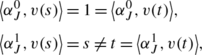
  so the vectors v(s), v(t) are linearly independent.

  For s,t∈ℝ, define

  $$r_X(s, t) :=\mathbb {C}\mathrm {ov}\bigl[X(s), X(t)\bigr], \qquad \sigma^2_X(t) := \mathbb {V}\mathrm {ar}\bigl[X(t)\bigr] = r_X(t, t). $$

  Then, if s,t∈[−K,K],

  

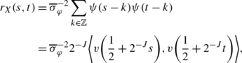
  so by Cauchy-Schwarz,

  $$r_X(s, t)^2 < \sigma_X^2(s) \sigma_X^2(t). $$

  If s,t∈[k−K,k+K] for some k∈ℤ, the same applies by cyclostationarity. If not, then as φ is supported on [1−K,K], we have r _X (s,t)=0. However, for any t∈[0,1], $\langle\alpha^{1}_{J}, v(\frac{1}{2} + 2^{-J}t) \rangle= 1$, so

  $$\sigma_X^2(t) = \overline {\sigma }_{\varphi }^{-2} 2^{-J} \bigl \Vert v(t)\bigr \Vert ^2 > 0, $$

  and by cyclostationarity the same holds for all t∈ℝ. We thus again obtain

  $$r_X(s, t)^2 < \sigma_X^2(s) \sigma_X^2(t). $$

• (iii) We have

  $$\sigma_X^2(t) = \overline {\sigma }_{\varphi }^{-2} \sigma_{\varphi}^2(t), $$

  so by Assumption 2.2, $\sup_{t \in[0,1]} \sigma_{X}^{2}(t) = 1$, and this maximum is attained at a unique t ₀∈[0,1). If t ₀∈(0,1), this satisfies the conditions of the theorem directly; if not we may proceed as in Proposition 9 of Giné and Nickl [9]. $\sigma_{\varphi}^{2}$ is twice differentiable,

  $$2\overline {\sigma }_{\varphi }\sigma_X'(t_0) = \bigl( \sigma_{\varphi}^2\bigr)'(t_0) \sigma_{\varphi}^2(t_0)^{-1/2} = 0, $$

  and

  

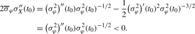
  Finally, let v′(t) denote the vector $(\varphi'_{J,k}(t)) \in \mathbb{R}^{\mathbb{Z}}$. Then for t∈[0,1],

  $$\bigl\langle\alpha^1_J, v'(t) \bigr \rangle= f_1'(t) = 1, $$

  so

  

  (4.1)

• (iv) Since φ has support [1−K,K],

  $$\sup_{s,t:\vert s-t \vert \ge2K-1} \bigl \vert r_X(s, t) \bigr \vert = 0. $$

 □

We may now bound the variance of $\hat {f}(j_{n})$. We will show that the variance process is distributed as the process X from the above lemma, so can be controlled similarly.

Proof of Theorem 2.3

Let $I_{n} :=[0, 2^{j_{n}}]$. The process

$$X_n(t) :=\frac{\hat {f}(j_n) - \bar {f}(j_n)}{c(j_n)}\bigl(2^{-j_n}t\bigr), \quad t \in I_n, $$

is distributed as

$$\overline {\sigma }_{\varphi }^{-1}2^{-j_n/2} \Biggl( \sum_{k\in K_{j_0}} Z_{j_0,k} \varphi_{j_0,k}\bigl(2^{-j_n}t\bigr) + \sum _{j = j_0}^{j_n-1} \sum _{k \in K_j} Z_{j,k} \psi_{j,k} \bigl(2^{-j_n}t\bigr) \Biggr) $$

for $Z_{j,k} \overset {\mathrm {i.i.d.}}{\sim }N(0, 1)$, so by an orthogonal change of basis, as

$$\overline {\sigma }_{\varphi }^{-1} 2^{-j_n/2} \sum_{k\in K_{j_n}} Z_k \varphi_{j_n,k}\bigl(2^{-j_n}t\bigr), \quad Z_k \overset {\mathrm {i.i.d.}}{\sim }N(0, 1). $$

For a regular wavelet basis, X _n is distributed on I _n as the process X from Lemma A.2, so we are done.

For a basis on the interval, set $J_{n} :=[2K, 2^{j_{n}} - 2K]$, and K _n :=I _n ∖J _n . On J _n , X _n is distributed as the process X from Lemma A.2, and we have

so for u _n (j _n ):=x(γ _n )/a(j _n )+b(j _n ),

For X _n to be large on K _n , one of the 4K variables

$$Z_k,\quad k \in\bigl\{0, \dots, 2K-1, 2^{j_n}-2K, \dots, 2^{j_n}-1\bigr\}, $$

must be large. Thus, by a simple union bound, for a constant C>0 depending on φ, the above probability is at most

$$8K\varPhi\bigl(-Cu_n(j_n)\bigr) \lesssim e^{-C^2u_n(j_n)^2/2}/u_n(j_n) = o(\gamma_n). $$

The result then follows by Lemma A.2, applied to the process X on J _n . □

References

Bickel, P.J., Rosenblatt, M.: On some global measures of the deviations of density function estimates. Ann. Stat. 1, 1071–1095 (1973)
Brown, L.D., Low, M.G.: Asymptotic equivalence of nonparametric regression and white noise. Ann. Stat. 24(6), 2384–2398 (1996). doi:10.1214/aos/1032181159
Bull, A.D.: Honest adaptive confidence bands and self-similar functions. Electron. J. Stat. 6, 1490–1516 (2012). doi:10.1214/12-EJS720
Bull, A.D.: Source code for a Smirnov–Bickel–Rosenblatt theorem for compactly supported wavelets (2011). arXiv:1110.4961
Chyzak, F., Paule, P., Scherzer, O., Schoisswohl, A., Zimmermann, B.: The construction of orthonormal wavelets using symbolic methods and a matrix analytical approach for wavelets on the interval. Exp. Math. 10(1), 67–86 (2001)
Cohen, A., Daubechies, I., Vial, P.: Wavelets on the interval and fast wavelet transforms. Appl. Comput. Harmon. Anal. 1(1), 54–81 (1993). doi:10.1006/acha.1993.1005
Daubechies, I.: Ten Lectures on Wavelets. CBMS-NSF Regional Conference Series in Applied Mathematics, vol. 61. SIAM, Philadelphia (1992)
Giné, E., Güntürk, C.S., Madych, W.R.: On the periodized square of L 2 cardinal splines. Exp. Math. 20(2), 177–188 (2011)
Giné, E., Nickl, R.: Confidence bands in density estimation. Ann. Stat. 38(2), 1122–1170 (2010). doi:10.1214/09-AOS738
Härdle, W., Kerkyacharian, G., Picard, D., Tsybakov, A.: Wavelets, Approximation, and Statistical Applications. Lecture Notes in Statistics, vol. 129. Springer, New York (1998)
Hüsler, J.: Extremes of Gaussian processes, on results of Piterbarg and Seleznjev. Stat. Probab. Lett. 44(3), 251–258 (1999). doi:10.1016/S0167-7152(99)00016-4
Hüsler, J., Piterbarg, V., Seleznjev, O.: On convergence of the uniform norms for Gaussian processes and linear approximation problems. Ann. Appl. Probab. 13(4), 1615–1653 (2003). doi:10.1214/aoap/1069786514
Piterbarg, V., Seleznjev, O.: Linear interpolation of random processes and extremes of a sequence of Gaussian nonstationary processes. Technical report 446, Department of Statistics, University of North Carolina, Chapel Hill, NC (1994)
Rioul, O.: Simple regularity criteria for subdivision schemes. SIAM J. Math. Anal. 23(6), 1544–1576 (1992). doi:10.1137/0523086
Smirnov, N.V.: On the construction of confidence regions for the density of distribution of random variables. Dokl. Akad. Nauk SSSR (N.S.) 74, 189–191 (1950)
Tsybakov, A.B.: Introduction to Nonparametric Estimation. Springer Series in Statistics. Springer, New York (2009)
Acknowledgements
We would like to thank Richard Nickl for his valuable comments and suggestions.
Author information
Authors and Affiliations
Corresponding author
Additional information
Communicated by G. Kerkyacharian.