Approximation of Analytic Sets with Proper Projection by Algebraic Sets

Abstract

Let X be an analytic subset of U×C ⁿ of pure dimension k such that the projection of X onto U is a proper mapping, where U⊂C ^k is a Runge domain. We show that X can be approximated by algebraic sets. Next we present a constructive method for local approximation of analytic sets by algebraic ones.

1 Introduction

The problem of polynomial approximation of holomorphic mappings has been thoroughly studied by several mathematicians (see a survey article [20] by N. Levenberg and the list of references therein).

In many cases, a holomorphic map f, for which approximations are looked for, is given implicitly; i.e., the graph of f (contained in some open set U⊂C ^m) is defined by $\operatorname{graph}(f)=\{F=0\}$, where F:U→C ^q is another holomorphic map. This leads to a generalization of the above mentioned problem by asking whether analytic sets can be constructively approximated by algebraic sets. An important motivation for such a question comes from algebraic geometry, where computational methods have been rapidly developed in recent years (see the book [15] by G.-M. Greuel and G. Pfister and references therein). These methods could be transferred to analytic geometry if one could suitably approximate analytic sets by algebraic ones.

The aim of the present paper is to show that every purely k-dimensional analytic subset of U×C ⁿ whose projection onto U is a proper mapping, where U is a Runge domain in C ^k, can be approximated by purely k-dimensional algebraic sets (see Theorem 3.1). Here, by a Runge domain we mean a domain of holomorphy U⊂C ^k such that every function $f\in\mathcal {O}(U)$ can be uniformly approximated on every compact subset of U by polynomials in k complex variables (cf. [16], pp. 36, 52). The approximation is expressed in terms of the convergence of holomorphic chains; i.e., analytic sets are treated as holomorphic chains with components of multiplicity one (see Sect. 2.2). (In the considered context, the convergence of holomorphic chains could be equivalently replaced by the convergence of the currents of integration over analytic sets (see [12], pp. 141, 206–207).)

One of the direct consequences of Theorem 3.1 is the existence of local algebraic approximations for every purely dimensional analytic set. This is because, due to Noether normalization, for every point of such a set X there is a neighborhood U such that X∩U is with proper projection onto an open subset of some linear space of dimension dimX (see Corollary 3.7).

Proving Theorem 3.1, we considerably strengthen the results of [4, 5], where it is shown that purely k-dimensional analytic subsets of U×C ⁿ with proper projection onto a Runge domain U⊂C ^k can be approximated by complex Nash sets. The latter fact is the starting point for our considerations. More precisely, it allows us to reduce the proof of Theorem 3.1 to the case where the approximated object is a complex Nash set. The problem in the reduced case is solved by Proposition 3.2. This proposition states that algebraic approximation of such a set is possible under milder hypotheses than those of Theorem 3.1, and therefore it is of independent interest. (In particular, the assumption that the approximated Nash set is an analytic cover is not necessary here.)

In the last section, a constructive method for local approximation of analytic sets by algebraic ones is given. The method is based on three main tools. These are a theorem on constructive approximation of holomorphic maps whose domains are Markov’s sets by J.-P. Calvi and N. Levenberg [11] (see also [10]), (constructive) normalization of algebraic sets for which the reader is referred to a book [15] by G.-M. Greuel and G. Pfister, and constructive approximation of analytic sets by Nash ones as described in [5].

Let us finish the introduction by recalling that the number q of equations defining an analytic set X={x∈U:F ₁(x)=⋯=F _q (x)=0}, where U is an open subset of C ^m, may be greater than the codimension of X in C ^m. In particular, there exist analytic sets defined (even locally) only by such “overdetermined” systems of equations. (An example of an analytic set for which there does not exist a description such that the number of defining functions equals the codimension of the set is given in [3], pp. 58–59.) In such a case, algebraic sets of the form $\{x\in U:\tilde{F}_{1}(x)=\cdots=\tilde{F}_{q}(x)=0\}$, where $\tilde{F}_{i}$ is any polynomial approximating F _i , are not good approximations for X because their dimension is usually smaller than required. For this reason, the problem of algebraic approximation of analytic sets is not a straightforward generalization of the problem of polynomial approximation of holomorphic maps, and new methods are necessary.

The organization of this paper is as follows. In Sect. 2, preliminary material is presented. Section 3 contains the proofs of Theorem 3.1 and Proposition 3.2. In the last section, we give a constructive procedure for local approximation of analytic sets and illustrate it by an example.

2 Preliminaries

2.1 Nash Sets

Let Ω be an open subset of C ⁿ, and let f be a holomorphic function on Ω. We say that f is a Nash function at x ₀∈Ω if there exist an open neighborhood U of x ₀ and a polynomial P:C ⁿ×C→C, P≠0, such that P(x,f(x))=0 for x∈U. A holomorphic function defined on Ω is said to be a Nash function if it is a Nash function at every point of Ω. A holomorphic mapping defined on Ω with values in C ^N is said to be a Nash mapping if each of its components is a Nash function.

A subset Y of an open set Ω⊂C ⁿ is said to be a Nash subset of Ω if and only if for every y ₀∈Ω there exists a neighborhood U of y ₀ in Ω and there exist Nash functions f ₁,…,f _s on U such that

$$Y\cap U=\bigl\{x\in U: f_1(x)=\cdots=f_s(x)=0\bigr\}.$$

The fact from [28] stated below explains the relation between Nash and algebraic sets.

Theorem 2.1

Let X be an irreducible Nash subset of an open set Ω⊂C ⁿ. Then there exists an algebraic subset Y of C ⁿ such that X is an analytic irreducible component of Y∩Ω. Conversely, every analytic irreducible component of Y∩Ω is an irreducible Nash subset of Ω.

2.2 Convergence of Closed Sets and Holomorphic Chains

Let U be an open subset in C ^m. By a holomorphic chain in U, we mean the formal sum A=∑ _j∈J α _j C _j , where α _j ≠0 for j∈J are integers and {C _j } _j∈J is a locally finite family of pairwise distinct irreducible analytic subsets of U (see [29], cp. also [2, 12]). The set ⋃ _j∈J C _j is called the support of A and is denoted by |A|, whereas the sets C _j are called the components of A with multiplicities α _j . The chain A is called positive if α _j >0 for all j∈J. If all the components of A have the same dimension n, then A will be called an n-chain.

Below we introduce the convergence of holomorphic chains in U. To do this, we first need the notion of the local uniform convergence of closed sets. Let Y,Y _ν be closed subsets of U for ν∈N. We say that {Y _ν } converges to Y locally uniformly if:

• (1l) For every a∈Y there exists a sequence {a _ν } such that a _ν ∈Y _ν and a _ν →a in the standard topology of C ^m.

• (2l) For every compact subset K of U such that K∩Y=∅, it holds that K∩Y _ν =∅ for almost all ν.

Then we write Y _ν →Y. For details concerning the topology of local uniform convergence see [30].

We say that a sequence {Z _ν } of positive n-chains converges to a positive n-chain Z if:

• (1c) |Z _ν |→|Z|.

• (2c) For each regular point a of |Z| and each submanifold T of U of dimension m−n transversal to |Z| at a such that $\overline{T}$ is compact and $|Z|\cap\overline{T}=\{a\}$, we have deg(Z _ν ⋅T)=deg(Z⋅T) for almost all ν.

Then we write Z _ν ↣Z. (By Z⋅T we denote the intersection product of Z and T (cf. [29]). Observe that the chains Z _ν ⋅T and Z⋅T for sufficiently large ν have finite supports and the degrees are well defined. Recall that for a chain $A=\sum_{j=1}^{d}\alpha_{j}\{a_{j}\}$, $\deg(A)=\sum_{j=1}^{d}\alpha_{j}$).

2.3 Normalization of Algebraic Sets

Let us recall that every affine algebraic set, regarded as an analytic set, has an algebraic normalization (see [21], p. 471). Therefore (in view of the basic properties of normal spaces, see [21], pp. 337, 343), the following theorem, which will be useful in the proof of the main result, holds true.

Theorem 2.2

Let $\tilde{Y}$ be an algebraic subset of C ^m. Then there are an integer n and an algebraic subset Z of C ^m×C ⁿ with $\pi(Z)=\tilde{Y}$, where π:C ^m×C ⁿ→C ^m is the natural projection, satisfying the following properties:

• (01) Z, regarded as an analytic set, is locally irreducible.

• (02) π| _Z :Z→C ^m is a proper map.

• (03) $\pi|_{Z\cap(\pi^{-1}(\tilde{Y}\setminus \operatorname{Sing}(\tilde{Y})))}:Z\cap(\pi^{-1}(\tilde{Y}\setminus \operatorname{Sing}(\tilde{Y})))\rightarrow\tilde{Y}$ is an injective map.

2.4 Runge Domains

We say that P is a polynomial polyhedron in C ⁿ if there exist polynomials in n complex variables q ₁,…,q _s and real constants c ₁,…,c _s such that

$$P=\bigl\{x\in\mathbf{C}^n:\bigl|q_1(x)\bigr|\leq c_1,\ldots,\bigl|q_s(x)\bigr|\leq c_s\bigr\}.$$

The following lemma is a straightforward consequence of Theorem 2.7.3 and Lemma 2.7.4 from [16].

Lemma 2.3

Let Ω⊂C ⁿ be a Runge domain. Then for every Ω ₀⋐Ω, there exists a compact polynomial polyhedron P⊂Ω such that $\varOmega_{0}\Subset \operatorname{Int}P$.

Theorem 2.7.3 from [16] immediately implies the following:

Claim 2.4

Let P be any polynomial polyhedron in C ⁿ. Then $\operatorname{Int}P$ is a Runge domain in C ⁿ.

The following fact from [16] (Theorem 2.7.7, p. 55) will also be useful to us.

Theorem 2.5

Let f be a holomorphic function in a neighborhood of a polynomially convex compact set K⊂C ⁿ. Then f can be uniformly approximated on K by polynomials in n complex variables.

3 Approximation of Analytic Sets

The following theorem is the first main result of this paper.

Theorem 3.1

Let U be a Runge domain in C ^k, and let X be an analytic subset of U×C ⁿ of pure dimension k with proper projection onto U. Then there is a sequence {X _ν } of algebraic subsets of C ^k×C ⁿ of pure dimension k such that {X _ν ∩(U×C ⁿ)} converges to X in the sense of holomorphic chains.

The proof of Theorem 3.1 is based on two results. First, every purely dimensional analytic set with proper and surjective projection onto a Runge domain can be approximated by Nash sets (a precise statement will be recalled later). Second, every complex Nash set with proper projection onto a Runge domain can be approximated by algebraic sets as stated in the following:

Proposition 3.2

Let Y be a Nash subset of Ω×C of pure dimension k<m, with proper projection onto Ω, where Ω is a Runge domain in C ^m−1. Then there is a sequence {Y _ν } of algebraic subsets of C ^m−1×C of pure dimension k such that {Y _ν ∩(Ω×C)} converges to Y in the sense of holomorphic chains.

Proof of Proposition 3.2

Let $\hat{l}$ be a positive integer, and let $\|\cdot\|_{\hat{l}}$ denote a norm in $\mathbf{C}^{\hat {l}}$. Set $B_{\hat{l}}(r)=\{x\in\mathbf{C}^{\hat{l}}:\|x\|_{\hat{l}}<r\}$. For any analytic subset X of an open subset of $\mathbf{C}^{\hat{l}}$, let X _(q) denote the union of all q-dimensional irreducible components of X.

To prove the proposition, it is clearly sufficient to show that for every open Ω ₀⋐Ω and for every real number r>0, the following holds:

• (*) There exists a sequence {Y _ν } of purely k-dimensional algebraic subsets of C ^m−1×C such that {Y _ν ∩(Ω ₀×B ₁(r))} converges to Y∩(Ω ₀×B ₁(r)) in the sense of chains.

Fix an open relatively compact subset Ω ₀ of Ω and a real number r>0. Let $\tilde{\pi}:\mathbf{C}^{m-1}\times\mathbf{C}\rightarrow\mathbf{C}^{m-1}$ denote the natural projection.

Claim 3.3

There exists a purely k-dimensional algebraic subset $\tilde{Y}$ of C ^m−1×C such that Y∩(Ω ₀×B ₁(r)) is the union of some of the analytic irreducible components of $\tilde{Y}\cap(\varOmega_{0}\times B_{1}(r))$. Moreover, the mapping $\tilde{\pi}|_{\tilde{Y}}:\tilde{Y}\rightarrow\mathbf{C}^{m-1}$ may be assumed to be proper.

Proof of Claim 3.3

By Lemma 2.3, we can fix a compact polynomial polyhedron P⊂Ω such that Ω ₀⋐Γ⋐Ω, where $\varGamma=\operatorname{Int}P$. The complex manifold $\operatorname{Reg}_{\mathbf{C}}(Y\cap(\varGamma\times\mathbf{C}))$ is a semi-algebraic subset of R ^2m, hence it has a finite number of connected components. Consequently, Y∩(Γ×C) has finitely many analytic irreducible components. Therefore, by Theorem 2.1 there exists a purely k-dimensional algebraic subset $\tilde{Y}$ of C ^m−1×C such that Y∩(Γ×C) is the union of some of the analytic irreducible components of $\tilde{Y}\cap(\varGamma\times\mathbf{C})$. Then, clearly, Y∩(Ω ₀×B ₁(r)) is the union of some of the analytic irreducible components of $\tilde{Y}\cap(\varOmega_{0}\times B_{1}(r))$.

If the mapping $\tilde{\pi}|_{\tilde{Y}}:\tilde{Y}\rightarrow\mathbf{C}^{m-1}$ is proper, then the proof is completed. Otherwise, using the facts that $Y\cap(\varGamma\times\mathbf{C})\subset\tilde{Y}\cap(\varGamma\times\mathbf{C})$ and Ω ₀⋐Γ, we show that there are a C-linear isomorphism Φ:C ^m→C ^m, a Runge domain Ω ₁ in C ^m−1, and a real number s>0 such that the following hold:

• (a) The projection of $\varPhi(\tilde{Y})\subset\mathbf{C}^{m-1}\times\mathbf{C}$ onto C ^m−1 is a proper mapping.

• (b) Φ(Ω ₀×B ₁(r))⊂Ω ₁×B ₁(s).

• (c) Φ(Y)∩(Ω ₁×B ₁(s)) is a Nash subset of Ω ₁×C whose projection onto Ω ₁ is a proper mapping.

• (d) Φ(Y)∩(Ω ₁×B ₁(s)) is the union of some of the irreducible components of $\varPhi(\tilde{Y})\cap(\varOmega_{1}\times B_{1}(s))$.

If there exists a sequence {Z _ν } of purely k-dimensional algebraic subsets of C ^m−1×C such that {Z _ν ∩(Ω ₁×B ₁(s))} converges to Φ(Y)∩(Ω ₁×B ₁(s)) in the sense of chains, then Y∩(Ω ₀×B ₁(r)) is approximated, in view of (b), by {Φ ⁻¹(Z _ν )∩(Ω ₀×B ₁(r))}. Moreover, (c) implies that Ω ₁ and Φ(Y)∩(Ω ₁×B ₁(s)) taken in place of Ω and Y, respectively, satisfy the hypotheses of Proposition 3.2. Since, in view of (a) and (d), $\varPhi(\tilde{Y})$ is a purely k-dimensional algebraic subset of C ^m−1×C with proper projection onto C ^m−1, containing Φ(Y)∩(Ω ₁×B ₁(s)), the proof of the claim is completed provided there are Φ, Ω ₁, and s satisfying (a), (b), (c), and (d).

Take Ω ₁ to be any Runge domain in C ^m−1 with Ω ₀⋐Ω ₁⋐Γ. (The existence follows by Lemma 2.3 and Claim 2.4.) Now, since $\dim(\tilde{Y})=k<m$, by the Sadullaev theorem (see [21], p. 389), the set $\mathcal{S}_{\tilde{Y}}$ of one-dimensional linear subspaces l of C ^m such that the projection of $\tilde{Y}$ along l onto the orthogonal complement l ^⊥ of l in C ^m is proper, is open and dense in the Grassmannian G ₁(C ^m). Consequently, for every ε>0, there is $l\in\mathcal{S}_{\tilde{Y}}$ so close to {0}^m−1×C that there is a C-linear isomorphism Φ _ε :C ^m→C ^m transforming l,l ^⊥ onto {0}^m−1×C, C ^m−1×{0}, respectively, such that

$$\|\varPhi_{\varepsilon}-\operatorname{Id}_{\mathbf{C}^m}\|<\varepsilon,$$

where $\operatorname{Id}_{\mathbf{C}^{m}}$ is the identity on C ^m.

Clearly, Φ=Φ _ε satisfies (a) (for every ε>0). Now, by the facts that Y is a Nash subset of Ω×C such that $\tilde{\pi}|_{Y}:Y\rightarrow\varOmega$ is a proper map and Ω ₁⋐Ω, there is a real number s>r such that

$$\bigl(\overline{\varOmega_1}\times\partial B_1(s)\bigr)\cap Y=\emptyset.$$

This implies that Φ=Φ _ε satisfies (c) if ε is sufficiently small. Next, the facts Ω ₀⋐Ω ₁ and s>r imply that Φ=Φ _ε satisfies (b) for small ε. Finally, by Ω ₁⋐Γ, we get $\varPhi_{\varepsilon}^{-1}(\varOmega_{1}\times B_{1}(s))\subset\varGamma\times\mathbf{C}$ if ε is small enough. Therefore,

$$\varPhi_{\varepsilon}(Y)\cap\bigl(\varOmega_1\times B_1(s)\bigr)\subset\varPhi_{\varepsilon}(\tilde{Y})\cap\bigl(\varOmega_1\times B_1(s)\bigr),$$

which easily implies that (d) is satisfied with Φ=Φ _ε . Thus the proof is completed. □

Proof of Proposition 3.2 (continuation)

By Theorem 2.2, there are an integer n and a locally irreducible (regarded as an analytic space), purely k-dimensional algebraic subset Z of C ^m×C ⁿ such that the restriction π| _Z of the natural projection π:C ^m×C ⁿ→C ^m is a proper mapping, $\pi(Z)=\tilde{Y}$ and

$$\pi|_{Z\cap(\pi^{-1}(\tilde{Y}\setminus \operatorname{Sing}(\tilde{Y})))}:Z\cap\bigl(\pi^{-1}\bigl(\tilde{Y}\setminus \operatorname{Sing}(\tilde{Y})\bigr)\bigr)\rightarrow\tilde{Y}$$

is an injective mapping.

We may assume that $(\tilde{Y}\setminus Y)\cap(\varOmega\times\mathbf{C})\neq\emptyset$, because otherwise

$$Y\cap\bigl(\varOmega_0\times B_1(r)\bigr)=\tilde{Y}\cap \bigl(\varOmega_0\times B_1(r)\bigr),$$

and one can take $Y_{\nu}=\tilde{Y}$ for every ν∈N.

Now, the Nash subsets E and F of Ω×C×C ⁿ defined by

$$E=\bigl(Z\cap\pi^{-1}(Y)\bigr)_{(k)} \quad \mbox{and}\quad F=\bigl(Z\cap\pi^{-1}(\overline{\tilde{Y}\setminus Y})\cap\bigl(\varOmega \times\mathbf{C}\times\mathbf{C}^n\bigr)\bigr)_{(k)},$$

where the closure is taken in Ω×C, satisfy E∩F=∅. Indeed, if there exists some a∈E∩F, then Z (regarded as an analytic space) is not irreducible at a because

$$Z\cap\bigl(\varOmega\times\mathbf{C}\times\mathbf{C}^n\bigr)=E\cup F,$$

and dim(E∩F)<k. Consequently, the sets

$$\tilde{E}=E\cap\bigl(P\times\mathbf{C}\times\mathbf{C}^n\bigr) \quad \mbox{and}\quad \tilde{F}=F\cap\bigl(P\times\mathbf{C}\times\mathbf{C}^n\bigr)$$

also satisfy $\tilde{E}\cap\tilde{F}=\emptyset$, where P⊂Ω is a fixed compact polynomial polyhedron such that Ω ₀⊂P. (The existence of P follows by Lemma 2.3.)

By Claim 3.3, we may assume that the mapping $\tilde{\pi}|_{\tilde{Y}}$ is proper. Then the mapping $\hat{\pi}|_{Z}:Z\rightarrow\mathbf{C}^{m-1}$ is proper as well, where $\hat{\pi}=\tilde{\pi}\circ\pi$. This implies that both $\tilde{E}$ and $\tilde{F}$ are compact. Moreover, the mapping $(\hat{\pi},p)|_{Z}:Z\rightarrow\mathbf{C}^{m}$ is proper for every polynomial p:C ^m×C ⁿ→C.

Now the idea of the proof is to find a sequence {p _ν } of polynomials defined on C ^m×C ⁿ with the following properties:

• (0) $\{p_{\nu}|_{\tilde{E}}\}$ converges uniformly to the mapping (x ₁,…,x _m ,y ₁,…,y _n )↦x _m .

• (1) $\inf_{b\in\tilde{F}}|p_{\nu}(b)|>r$ for almost all ν.

Then we show that the sequence $\{(\hat{\pi},p_{\nu})(Z)\}$ of purely k-dimensional algebraic subsets of C ^m is as required in the condition (*): $\{(\hat{\pi},p_{\nu})(Z)\cap(\varOmega_{0}\times B_{1}(r))\}$ converges to Y∩(Ω ₀×B ₁(r)) in the sense of chains.

Claim 3.4

There exists a sequence {p _ν } of polynomials in m+n complex variables, satisfying (0) and (1).

Proof of Claim 3.4

First, by the fact that $\tilde{E}\cap\tilde{F}=\emptyset$, there is an open subset U of C ^m×C ⁿ such that U=U ₁∪U ₂, where U ₁,U ₂ are open subsets of C ^m×C ⁿ, U ₁∩U ₂=∅, and $\tilde{E}\subset U_{1},\tilde{F}\subset U_{2}$.

Second, abbreviate (x,y)=(x ₁,…,x _m ,y ₁,…,y _n ) and note that the function f:U→C defined by f(x,y)=x _m on U ₁ and f(x,y)=r+1 on U ₂ is holomorphic.

Third, observe that, since Z is an algebraic subset of C ^m×C ⁿ with proper projection onto C ^m, and $\pi(Z)=\tilde{Y}$ is an algebraic subset of C ^m−1×C with proper projection onto C ^m−1, and P is a compact polynomial polyhedron in C ^m−1, the union $\tilde{E}\cup\tilde{F}$ is a compact polynomial polyhedron (and hence a polynomially convex compact set) in C ^m×C ⁿ. Indeed, there are closed bounded polydiscs P′⊂C,P″⊂C ⁿ such that

$$\tilde{E}\cup\tilde{F}=Z\cap\bigl(P\times P'\times P''\bigr),$$

and the right-hand side of the latter equation is clearly described by a finite number of inequalities of the form |Q(x,y)|≤c, where Q is a complex polynomial and c is a real constant (possibly equal to zero).

Lastly, since f is a holomorphic function in a neighborhood of a polynomially convex compact set $\tilde{E}\cup\tilde{F}$, it is sufficient to apply Theorem 2.5 to obtain a sequence {p _ν } of complex polynomials in m+n variables converging uniformly to f on $\tilde{E}\cup\tilde{F}$. Clearly, every such sequence satisfies (0) and (1). □

Proof of Proposition 3.2 (end)

Let {p _ν } be a sequence of polynomials satisfying the assertion of Claim 3.4. We check that the sequence {Y _ν } defined by

$$Y_{\nu}=(\hat{\pi},p_{\nu}) (Z),\quad \mbox{for\ }\nu\in \mathbf{N},$$

satisfies the condition (*), which is sufficient to complete the proof of Proposition 3.2.

Every Y _ν is a purely k-dimensional algebraic subset of C ^m because the mapping $(\hat{\pi},p_{\nu}):\mathbf{C}^{m}\times\mathbf{C}^{n}\rightarrow\mathbf{C}^{m}$ is polynomial, its restriction $(\hat{\pi},p_{\nu})|_{Z}$ is proper, and Z is a purely k-dimensional algebraic subset of C ^m×C ⁿ. Hence it remains to check that {Y _ν ∩(Ω ₀×B ₁(r))} converges to Y∩(Ω ₀×B ₁(r)) in the sense of chains.

To see that {Y _ν ∩(Ω ₀×B ₁(r))} converges to Y∩(Ω ₀×B ₁(r)) locally uniformly (cf. (1l) and (2l), Sect. 2.2), it is sufficient to observe that

$$Y_{\nu}\cap\bigl(\varOmega_0\times B_1(r)\bigr)=(\hat{\pi},p_{\nu}) (\tilde{E})\cap \bigl(\varOmega_0\times B_1(r)\bigr)$$

for ν large enough, whereas

$$Y\cap\bigl(\varOmega_0\times B_1(r)\bigr)=\pi(\tilde{E})\cap\bigl(\varOmega_0\times B_1(r)\bigr).$$

The first equality follows directly by (0), (1), and the definitions of $\tilde{E}$ and $\tilde{F}$. The latter one is an obvious consequence of the definition of $\tilde{E}$. Moreover, (0) implies that $(\hat{\pi},p_{\nu})|_{\tilde{E}}$ converges to $\pi|_{\tilde{E}}$ uniformly, which in turn implies that both (1l) and (2l) are satisfied.

To finish the proof, let us verify that {Y _ν ∩(Ω ₀×B ₁(r))} and Y∩(Ω ₀×B ₁(r)) satisfy (2c) (of Sect. 2.2). Suppose that it is not true. Then there exist a k-dimensional C-linear subspace l of C ^m−1×{0} and open balls C ₁,C ₂ in l,l ^⊥ respectively, where l ^⊥ denotes the orthogonal complement of l in C ^m, such that $\overline{C_{1}+C_{2}}\subset\varOmega_{0}\times B_{1}(r)$ and the following hold:

• (a) $Y\cap(\overline{C_{1}}+\partial C_{2})=\emptyset$ and $(\overline{\tilde{Y}\setminus Y})\cap\overline{(C_{1}+C_{2})}=\emptyset$.

• (b) Every fiber of the projection of Y∩(C ₁+C ₂) onto C ₁ is 1-element.

• (c) The generic fiber of the projection of Y _ν ∩(C ₁+C ₂) onto C ₁ is at least 2-element for infinitely many ν.

The existence of l⊂C ^m (and C ₁, C ₂) as above is a direct consequence of the assumption that (2c) does not hold. Since the projection of $\tilde{Y}\subset\mathbf{C}^{m-1}\times\mathbf{C}$ onto C ^m−1 is a proper mapping, the subspace l can be chosen in such a way that it is contained in C ^m−1×{0}.

The conditions (a), (b), and the facts that $\pi|_{Z\cap(\pi^{-1}(\tilde{Y}\setminus \operatorname{Sing}(\tilde{Y})))}$ is injective and π| _Z is proper imply that

$$Z\cap\bigl(({C_1}+{C_2})\times\mathbf{C}^n\bigr)=\operatorname{graph}(G),$$

where $G\in\mathcal{O}({C_{1}},C_{2}\times\mathbf{C}^{n})$. Consequently, by (0) and the inclusion l⊂C ^m−1×{0}, for ν large enough,

$$T_{\nu}:=(\hat{\pi},p_{\nu}) \bigl(\operatorname{graph}(G)\bigr)$$

is a k-dimensional analytic subset of C ₁+C ₂ whose projection onto C ₁ has 1-element fibers. Now, we show that, for almost all ν,

$$Y_{\nu}\cap(C_1+C_2)\subset T_{\nu},$$

which contradicts (c). The latter inclusion holds because, as observed previously, for large ν we have

$$Y_{\nu}\cap(C_1+ C_2)= (\hat{\pi},p_{\nu}) (\tilde{E})\cap(C_1+C_2).$$

Moreover, by (0), (a), and the fact that l⊂C ^m−1×{0}, the following holds:

$$(\hat{\pi},p_{\nu}) (\tilde{E})\cap(C_1+C_2)=(\hat{\pi},p_{\nu}) \bigl(\tilde {E}\cap\bigl(({C_1}+{C_2})\times\mathbf{C}^n\bigr)\bigr),$$

which implies the inclusion as

$$\tilde{E}\cap\bigl(({C_1}+{C_2})\times \mathbf{C}^n\bigr)\subset \operatorname{graph}(G).$$

Thus {Y _ν ∩(Ω ₀×B ₁(r))} and Y∩(Ω ₀×B ₁(r)) satisfy (2c), and the proof of Proposition 3.2 is completed. □

Proof of Theorem 3.1

Let us first recall that for analytic covers, there exist Nash approximations:

Theorem 3.5

Let U be a connected Runge domain in C ^k, and let X be an analytic subset of U×C ⁿ of pure dimension k with proper projection onto U. Then for every open relatively compact subset V of U there is a sequence of Nash subsets of V×C ⁿ of pure dimension k with proper projection onto V, converging to X∩(V×C ⁿ) in the sense of holomorphic chains.

Papers [4, 5] contain detailed proofs of Theorem 3.5. Here let us just mention that this theorem is related to the problem of approximation of holomorphic maps between complex (algebraic) spaces, for which the reader is referred to [1, 9, 13, 14, 18, 19, 25–27].

Let us return to the proof of Theorem 3.1. Fix a Runge domain U in C ^k and an analytic subset X of U×C ⁿ of pure dimension k with proper projection onto U. Clearly, in order to prove Theorem 3.1, it is sufficient to check the following:

Claim 3.6

For every open V⋐U, there exists a sequence {X _ν } of purely k-dimensional algebraic subsets of C ^k×C ⁿ such that {X _ν ∩(V×C ⁿ)} converges to X∩(V×C ⁿ) in the sense of chains.

Let us prove the claim. Fix an open V⋐U. Since, without loss of generality, V can be replaced by a larger relatively compact Runge subdomain of U (cf. Sect. 2.4), we may assume that V is a Runge domain. By Theorem 3.5, there is a sequence {T _ν } of purely k-dimensional Nash subsets of V×C ⁿ, with proper projection onto V, converging to X∩(V×C ⁿ) in the sense of chains. (Formally in Theorem 3.5, U is assumed to be connected, but this assumption can be easily omitted by treating every connected component of U separately.)

For every ν, by Proposition 3.2 applied with Y=T _ν , Ω=V×C ⁿ⁻¹, and m=n+k, there is a sequence {Y _ν,μ } of algebraic subsets of C ^k×C ⁿ of pure dimension k such that {Y _ν,μ ∩(V×C ⁿ)} converges to T _ν in the sense of chains. Clearly, there is a function α:N→N such that {Y _ν,α(ν)∩(V×C ⁿ)} converges to X∩(V×C ⁿ). Thus the proofs of Claim 3.6 and Theorem 3.1 are completed. □

An immediate consequence of Theorem 3.1 is the following:

Corollary 3.7

Let X be a purely k-dimensional analytic subset of some open Ω⊂C ^m. Then for every a∈X, there are an open neighborhood U of a in Ω and a sequence {X _ν } of purely k-dimensional algebraic subsets of C ^m such that {X _ν ∩U} converges to X∩U in the sense of holomorphic chains.

Proof

Every point of a purely k-dimensional analytic subset X of some open Ω⊂C ^m has a neighborhood U⊂Ω such that, after a linear change of the coordinates, the projection of X∩U onto an open ball in C ^k×{0}^m−k is a proper mapping. Then, having applied Theorem 3.1, we obtain the corollary. □

4 Constructive Approximation of Analytic Sets

Let X be a purely k-dimensional analytic subset of an open set Ω⊂C ^m such that 0∈X. Our aim is to construct a sequence {X _ν } of purely k-dimensional algebraic subsets of C ^m such that {X _ν ∩Ω ₀} converges to X∩Ω ₀ in the sense of chains for some open neighborhood Ω ₀ of 0∈C ^m and, moreover, every irreducible component E of X∩Ω ₀ is the limit of a sequence {E _ν }, where E _ν is an analytic irreducible component of X _ν ∩Ω ₀. The construction is based on the proof of Theorem 3.1 and for that reason we need constructive versions of Theorem 2.5 and Theorem 2.2 involved in the proof (details below).

Let us first prepare the setup. Applying a linear change of the coordinates and shrinking Ω, if necessary, we assume that Ω=U×B, where U,B are open balls in C ^k, C ⁿ respectively, m=k+n, and the projection of X onto U is a proper map. Then, for some integer r, there exist polynomials $p_{1},\ldots,p_{r}\in\mathcal{O}(U)[z_{1},\ldots,z_{n}]$, such that

$$X=\bigl\{(x,z_1,\ldots,z_n)\in U\times \mathbf{C}^n: p_1(x,z_1,\ldots ,z_n)=\cdots=p_r(x,z_1,\ldots,z_n)=0\bigr\}.$$

(For example, p ₁,…,p _r may be the canonical defining functions of X, so one may also assume that Ω=U×C ⁿ.) The functions p ₁,…,p _r constitute the input for our method.

Before presenting the details, let us briefly sketch the idea of the construction of X _ν . The first stage is to construct a purely k-dimensional algebraic subset $\tilde{X}_{\nu}$ of C ^m with the following properties. For some open connected neighborhood U ₀⋐U of 0 (independent of ν), every irreducible component of X∩(U ₀×C ⁿ) is approximated by some analytic irreducible component of $\tilde{X}_{\nu}\cap (U_{0}\times\mathbf{C}^{n})$. Moreover, $\tilde{X}_{\nu}\subset\mathbf{C}^{k}\times\mathbf{C}^{n}\approx\mathbf{C}^{m}$ is with proper projection onto C ^k. Steps 1–4 of the procedure (written below) are responsible for this first stage. (Note that $\tilde{X}_{\nu}\cap(U_{0}\times\mathbf{C}^{n})$ may contain irreducible components not corresponding to any irreducible components of X∩(U ₀×C ⁿ), so in further steps $\tilde{X}_{\nu}$ will have to be modified so that these additional components can be removed.)

The fact that $\tilde{X}_{\nu}$, defined in Step 4, is with proper projection onto C ^k is a consequence of $\tilde{q}_{i}$ being unitary in z _i for i=1,…,n. Let us explain that $\tilde{X}_{\nu}$ has the other required properties. For i∈{1,…,n}, define

$$q_{i,\nu}(x,z_i):=z^{n_i}_i+z^{n_i-1}_ia_{i,1,\nu}(x)+\cdots + a_{i,n_i,\nu}(x),$$

where $a_{i,1,\nu},\ldots,a_{i,n_{i},\nu}:C_{0}\rightarrow\mathbf{C}$ are Nash functions described in Step 3, and let q _i (x,z _i ) be the polynomial defined in Step 1. Next we write

and take any open U ₀⋐C ₀ containing zero. By Steps 1–3, we can invoke Theorem 3.1 of [5] (with X=W,X _ν =W _ν ), which implies that every analytic irreducible component of W∩(U ₀×C ⁿ) is approximated by some analytic irreducible component of W _ν ∩(U ₀×C ⁿ) (if a _i,j,ν is close to a _i,j for every i∈{1,…,n},j∈{1,…,n _i }). Now, X∩(U ₀×C ⁿ)⊂W∩(U ₀×C ⁿ), and $W_{\nu}\cap(U_{0}\times\mathbf{C}^{n})\subset\tilde{X}_{\nu}\cap(U_{0}\times \mathbf{C}^{n})$, and all these sets are purely k-dimensional, which imply that $\tilde{X}_{\nu}$ has all the required properties.

Given $\tilde{X}_{\nu}$, we follow the proof of Proposition 3.2 with Ω=U ₀×C ⁿ⁻¹ and Y taken to be the union of those analytic irreducible components of $\tilde{X}_{\nu}\cap(U_{0}\times\mathbf{C}^{n})$ for which Y approximates X∩(U ₀×C ⁿ). More precisely, the situation is now simpler than in Proposition 3.2 because $\tilde{X}_{\nu}\subset\mathbf{C}^{k}\times\mathbf{C}^{n}$ is with proper projection onto C ^k. Consequently, no global coordinate changes are necessary. We just proceed by computing a purely k-dimensional algebraic subset Z _ν of C ^k×C ⁿ×C ^d, for some d∈N, such that Z _ν is a locally irreducible analytic set, $\pi|_{Z_{\nu}}$ is a proper map, and $\pi(Z_{\nu})=\tilde{X}_{\nu}$, where π:C ^k×C ⁿ×C ^d→C ^k×C ⁿ is the natural projection (Step 5).

By the proof of Proposition 3.2, we know that Z _ν ∩(U ₀×C ⁿ×C ^d)=E _ν ∪F _ν , where E _ν ,F _ν are purely k-dimensional Nash sets such that π(E _ν ) approximates X∩(U ₀×C ⁿ) and E _ν ,F _ν are separated from each other. In the last step, we replace π by a polynomial map π _ν such that X _ν =π _ν (Z _ν ) is an algebraic set approximating X as described in the first paragraph of this section (where Ω ₀=U ₀×C ⁿ). To this end, π _ν is chosen in such a way that π _ν (E _ν ) is close to π(E _ν ), whereas π _ν (Z _ν ∖E _ν )∩(U ₀×B _n (ν))=∅, where B _n (ν) is the ball in C ⁿ centered at zero with radius ν.

Let us present the details. For hints on how the approximation can be carried out in practice, see the paragraphs following the procedure below. Let X,p ₁,…,p _r be as in the second paragraph of this section.

Construction of X _ν

• 1. For every i∈{1,…,n}, compute the unitary polynomial

  $$q_i=z_i^{n_i}+z_i^{n_i-1}a_{i,1}+\cdots +a_{i,n_i}\in\mathcal{O}(U)[z_i],$$

  with nonzero discriminant such that π _i (X)={(x,z _i )∈U×C _i :q _i (x,z _i )=0}, where $\pi_{i}:U\times\mathbf{C}^{n}_{z_{1},\ldots,z_{n}}\rightarrow U\times\mathbf{C}_{z_{i}}$ is the natural projection.

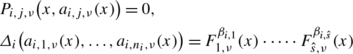
• 2. For every i∈{1,…,n}, compute the discriminant $\varDelta_{i}\in\mathbf{C}[a_{i,1},\ldots,a_{i,n_{i}}]$ of q _i . Next find functions $F_{1},\ldots,F_{\hat{s}}$ holomorphic in some neighborhood of 0∈C ^k such that for every i∈{1,…,n},

  $$\varDelta_i\bigl(a_{i,1}(x),\ldots,a_{i,n_i}(x)\bigr)=F_1^{\beta_{i,1}}(x)\cdot\cdots \cdot F_{\hat{s}}^{\beta_{i,\hat{s}}}(x),$$

  where $\beta_{i,1},\ldots,\beta_{i,\hat{s}}$ is a sequence of nonnegative integers; moreover, for every $l\in\{1,\ldots,\hat{s}\}$, {F _l =0} has no multiple irreducible components, and for every $j,l\in\{1,\ldots,\hat{s}\}$ with j≠l, {F _j =0} and {F _l =0} have no common irreducible components.

• 3. For every i∈{1,…,n}, j∈{1,…,n _i }, introduce a new variable $\tilde{z}_{i,j}$ and construct a nonzero polynomial $P_{i,j,\nu}\in(\mathbf{C}[x])[\tilde{z}_{i,j}]$ of degree in $\tilde{z}_{i,j}$ independent of ν, unitary in $\tilde{z}_{i,j}$ such that there are Nash functions a _i,j,ν , $F_{1,\nu},\ldots, F_{\hat{s},\nu}$ approximating uniformly $a_{i,j}, F_{1},\ldots, F_{\hat{s}}$ on an open neighborhood C ₀ of zero (independent of ν), and

  

  for every x∈C ₀. Such a construction is described in detail in [5] (p. 327).

• 4. For every i∈{1,…,n}, let $\tilde{q}_{i}$ be the polynomial obtained by replacing every coefficient a _i,j of q _i (except for the coefficient 1 standing at $z_{i}^{n_{i}}$) by the variable $\tilde{z}_{i,j}$ (appearing in P _i,j,ν ). Now let $\tilde{X}_{\nu}$ be the image of the projection of the algebraic set

  $$V_{\nu}=\{\tilde{q}_i=0, P_{i,j,\nu}=0, \mbox{ for }i=1,\ldots,n \mbox{ and } j=1,\ldots, n_i\}$$

  onto $\mathbf{C}^{k}_{x}\times\mathbf{C}^{n}_{z_{1}\ldots z_{n}}$. Hence the equations defining $\tilde{X}_{\nu}$ can be obtained by eliminating $\tilde{z}_{i,j}$’s from the equations defining V _ν .

• 5. For some d∈N, compute a purely k-dimensional algebraic subset Z _ν of C ^k×C ⁿ×C ^d locally irreducible as an analytic set such that $\pi|_{Z_{\nu}}$ is a proper map and $\pi(Z_{\nu})=\tilde{X}_{\nu}$, where π:C ^k×C ⁿ×C ^d→C ^k×C ⁿ is the natural projection. Let U ₀⋐C ₀ be an open polydisc containing 0∈C ^k, and let $\overline{U_{0}}$ be its closure in C ₀. Then $Z_{\nu}\cap(\overline{U_{0}}\times\mathbf{C}^{n}\times\mathbf{C}^{d})=\tilde {E_{\nu}}\cup \tilde{F_{\nu}}$, where $\tilde{E_{\nu}}, \tilde{F_{\nu}}$ are compact sets such that $\tilde{E_{\nu}}\cap\tilde{F_{\nu}}=\emptyset$. Moreover, $E_{\nu}={\tilde{E}_{\nu}}\cap(U_{0}\times\mathbf{C}^{n}\times\mathbf{C}^{d})$ is a purely k-dimensional Nash set such that π(E _ν ) approximates X∩(U ₀×C ⁿ).

• 6. Compute a polynomial map Q _ν :C ^k×C ⁿ×C ^d→C ⁿ approximating uniformly the natural projection $\check{\pi}:\mathbf{C}^{k}\times\mathbf{C}^{n}\times\mathbf{C}^{d}\rightarrow \mathbf{C}^{n}$ on $\tilde{E_{\nu}}$ such that

  $$\inf_{x\in\tilde{F_{\nu}}}\bigl\|Q_{\nu}(x)\bigr\|_{\mathbf{C}^n}>\nu.$$

  Next compute $X_{\nu}=(\acute{\pi}, Q_{\nu})(Z_{\nu})$, where $\acute{\pi}:\mathbf{C}^{k}\times\mathbf{C}^{n}\times\mathbf{C}^{d}\rightarrow \mathbf{C}^{k}$ is the natural projection.  □

Before discussing how this construction could be carried out in practice, let us note that not every analytic function can constitute (a part of) input data. Only objects which can be encoded as finite sequences of symbols can be considered. A large class of sets for which approximation could be useful are algebraic (or Nash) sets described by polynomials of very high degrees. Then the task would be to find approximations of such sets described by polynomials of lower degrees. Also in many cases in which analytic sets are described by (compositions) of elementary analytic functions whose properties we know, the construction could be carried out quite fast.

In general, one could consider the model in which for every function f depending on the variables x ₁,…,x _k , there is a finite procedure $\operatorname{Expand}_{f}$ which for every tuple (n ₁,…,n _k )∈N ^k returns the coefficient of the Taylor expansion of f around zero, standing at $x_{1}^{n_{1}}\cdot\cdots\cdot x_{k}^{n_{k}}$. The input data corresponding to the function f consist of the procedure $\operatorname{Expand}_{f}$, the size of the polydisc neighborhood U _f of zero on which the Taylor expansion of f is convergent. Furthermore, |f| is assumed to be bounded on U _f , and we know the bound M _f .

Observe that having input data for two functions f,g, we can recover the corresponding data for f+g, f⋅g, and $\frac{1}{f}$ (the latter if f(0)≠0). If we could test whether f is identically zero, then we could carry out all the first three steps of the construction in which transcendental objects appear. (Step 2 requires some further explanations given below. For the moment, let us only note that, clearly, under these assumptions we would also have procedures for expansions of functions appearing in the Weierstrass preparation theorem).

Unfortunately, given only $\operatorname{Expand}_{f}$, U _f , M _f , it is not possible to test in a finite number of steps whether f=0. But for every ε>0, it is possible to check whether $\sup_{U_{f}}|f|<\varepsilon$; hence, we can pick small ε>0 at the beginning and every time $\sup_{U_{f}}|f|<\varepsilon$ assume that f=0. Of course, if f≠0, then the output may not be correct. If we have some extra information about X which allows us to exclude incorrect outputs X _ν , then we can repeat the procedure with smaller ε. In such a general model, however, the existence of “badly conditioned” problems seems to be inevitable.

Carrying out the construction in Steps 2, 5, and 6 requires further explanation. First, to compute $F_{1},\ldots,F_{\hat{s}}$ in Step 2, we may assume that in some neighborhood of zero for every i∈{1,…,n}, $\varDelta_{i}(a_{i,1}(x),\ldots ,a_{i,n_{i}}(x))=W_{i}(x)H_{i}(x)$, where H _i is a holomorphic function, H _i (0)≠0 and W _i is the unitary polynomial in x _k with holomorphic coefficients depending on x′=(x ₁,…,x _k−1) vanishing at 0∈C ^k−1. (Otherwise we apply a generic linear change of the variables in a neighborhood of 0∈C ^k and the Weierstrass preparation theorem.) We may write F ₁=H ₁,…,F _n =H _n . Now we are left to find holomorphic functions $F_{n+1},\ldots,F_{\hat{s}}$, whose zero sets have the properties specified in Step 2, such that for every i∈{1,…,n},

$$W_i=F_{n+1}^{\beta_{i,n+1}}\cdot\cdots\cdot F_{\hat{s}}^{\beta_{i,\hat{s}}},$$

where $\beta_{i,n+1},\ldots,\beta_{i,\hat{s}}$ is a sequence of nonnegative integers. Since every W _i is a unitary polynomial in x _k (with holomorphic coefficients), we can obtain $F_{n+1},\ldots,F_{\hat{s}}$ by applying the division algorithm for polynomials to the W _i ’s and their (higher order) partial derivatives with respect to x _k .

In Step 5, Z _ν can be effectively obtained, for example, by computing the normalization of $\tilde{X}_{\nu}$ (see [15] for the algorithm of normalization; the fact that the algebraic set Z _ν normalizing $\tilde{X}_{\nu}$ is a locally irreducible analytic set follows by the standard properties of normal spaces, see [21], pp. 337, 343, 471).

The fact that Step 6 is constructive is a direct consequence of the existence of an effective procedure for computing the polynomial map Q _ν . Let K ₁,K ₂ be any closed bounded neighborhoods of $\tilde{E_{\nu}}, \tilde{F_{\nu}}$, respectively, such that K ₁∩K ₂=∅. Observe that any polynomial map Q _ν sufficiently close (on K ₁∪K ₂) to the holomorphic map f:K ₁∪K ₂→C ⁿ given by $f|_{K_{1}}=\check{\pi}|_{K_{1}}$ and $f|_{K_{2}}=c$, where c∈C ⁿ, $\|c\|_{\mathbf{C}^{n}}>\nu$, is good for our purpose. Hence what we need is to construct K ₁∪K ₂ and approximate f.

The union K ₁∪K ₂ will be constructed in such a way that it satisfies Markov’s inequality. Then holomorphic functions defined on K ₁∪K ₂ can be constructively approximated by polynomials (see [11]). More precisely, an approximating polynomial $\tilde{g}$ (of a given degree) for a holomorphic function $g\in\mathcal{O}(K)$, where K is a Markov’s set, can be taken to be the one minimizing the sum $\sum_{c\in\tilde{K}}|g(c)-\tilde{g}(c)|^{2}$, where $\tilde{K}$ is a suitably chosen finite subset of K. (The cardinality of $\tilde{K}$ depends on the exponent in Markov’s inequality.) For details, the reader is referred to [11]. This method is related to the concept of using the Lagrange interpolating polynomials to approximate holomorphic functions (see [6–8, 24]).

As for constructing K ₁∪K ₂, one can take a special polynomial polyhedron, i.e., a set of the form

$$\bigl\{u\in\mathbf{C}^{k}\times\mathbf{C}^n\times \mathbf{C}^d: \bigl|g_1(u)\bigr|\leq1,\ldots,\bigl|g_{k+n+d}(u)\bigr|\leq1\bigr\},$$

where g ₁,…,g _k+n+d are complex polynomials in k+n+d variables such that $\{u\in\mathbf{C}^{k}\times\mathbf{C}^{n}\times\mathbf{C}^{d}:\hat {g}_{1}(u)=\cdots=\hat{g}_{k+n+d}(u)=0\}=\{0\}^{k+n+d}$, where $\hat{g}_{1},\ldots,\hat{g}_{k+n+d}$ are homogeneous polynomials with $\deg(g_{i})=\deg(\hat{g}_{i})$ and $\deg(g_{i}-\hat{g}_{i})<\deg(g_{i})$ for i=1,…,k+n+d. Using the techniques of [22] (pp. 369–374), one can construct a special polynomial polyhedron $\mathcal{P}$ such that $\tilde{E_{\nu}}\cup\tilde{F_{\nu}}\subset \mathcal{P}$ and $\tilde{E_{\nu}}\cup\tilde{F_{\nu}}$ is approximated (in the sense of the Hausdorff distance) by the union of some connected components of $\mathcal{P}$. When this approximation is close enough, then $\mathcal{P}$ decomposes as $\mathcal{P}=K_{1}\cup K_{2}$ where K ₁,K ₂ are compact sets such that $\tilde{E_{\nu}}\subset K_{1}$, $\tilde{F_{\nu }}\subset K_{2}$, and K ₁∩K ₂=∅. Let us recall that every special polynomial polyhedron satisfies Markov’s inequality. Moreover, for such a set, the formula for the Siciak extremal function is known (see [17], p. 37), which allows one to compute the Markov’s exponent (see [20], p. 129). (For other examples of Markov’s sets, see [23].)

Finally, let us consider the following:

Example

Define

$$Y=\bigl\{(x,y,z,w)\in\mathbf{C}^4:z^5-2f(x,y)e^{(\frac{x+y^2}{10})^{30}}=w^5+g(x,y)w-2f(x,y)=0\bigr\},$$

where

For any r>0, put K _r ={x∈C:|x|<r}. One can easily check that $\tilde{Y}=Y\cap(K_{1}\times K_{1}\times K_{1.4}\times K_{1.4})$ is a purely 2-dimensional analytic subset of K ₁×K ₁×K _1.4×K _1.4 with proper projection onto K ₁×K ₁, whose generic fiber over K ₁×K ₁ has 25 points. As we shall see, $\tilde{Y}$ is reducible.

Let X be the irreducible component of $\tilde{Y}$ such that

where for any B⊂C ⁿ and a=(a ₁,…,a _n )∈C ⁿ, $\operatorname{dist}(B,a)=\inf\{\|a-b\|:b\in B\}$, and ∥a∥=max _i=1,…,n |a _i |. We shall see subsequently that X has 5 points in the generic fiber over K ₁×K ₁.

Our aim is to construct an algebraic subset X ₁ of C ⁴ approximating X. More precisely, we shall construct p ₁,p ₂,p ₃∈C[x,y,z,w] such that

$$X_{1}=\bigl\{(x,y,z,w)\in\mathbf {C}^4:p_1(x,y,z,w)=p_2(x,y,z,w)=p_3(x,y,z,w)=0\bigr\},$$

and $\operatorname{dist}({X_{1}}\cap T,{X}\cap T)<5\cdot10^{-4}$, where T=K ₁×K ₁×K _1.14×K _1.4 and $\operatorname{dist}(M,N)=\max\{\sup_{m\in M}\operatorname{dist}(N,m),\sup_{n\in N}\operatorname{dist}(M,n)\}$. Moreover, every branch of X∩T will be approximated by precisely one branch of X ₁∩T (as required in the definition of the convergence of holomorphic chains).

Note that we are not given equations defining X and it does not seem to be easy to obtain these equations from the definition of X. However, in this example one does not need them to show (see below) that

where π _w ,π _z denote the natural projections of $\mathbf {C}^{4}_{xyzw}$ onto $\mathbf{C}^{3}_{xyw}$, $\mathbf{C}^{3}_{xyz}$, respectively, and to show that polynomials q _w ,q _z computed in the first step of the construction are q _w (x,y,w)=w ⁵+g(x,y)w−2f(x,y), $q_{z}(x,y,z)=z^{5}-2f(x,y)e^{(\frac {x+y^{2}}{10})^{30}}$.

In the second step, we compute and decompose the discriminants Δ _w ,Δ _z of q _w ,q _z to obtain

where h(x,y)=x+2.2⋅10⁻³ y+10⁻³⁰ x ¹⁵⁰⁰cos(y), $a(x,y)=2f(x,y)e^{(\frac{x+y^{2}}{10})^{30}}$, and $(g_{z}^{-1}(0)\cup g_{w}^{-1}(0))\cap(K_{1}\times K_{1})=\emptyset$.

In the third step, we approximate h,g _z ,g _w ,a,f,g by Nash functions h ₁,g _z,1, g _w,1,a ₁,f ₁,g ₁ in such a way that the equations

are satisfied. Then $\tilde{Y}_{1}=\{(x,y,w,z)\in K_{1}\times K_{1}\times K_{1.4}\times K_{1.4}:z^{5}-a_{1}(x,y)=w^{5}+g_{1}(x,y)w-2f_{1}(x,y)=0\}$ has the following property. Every irreducible component of $\tilde{Y}$ is approximated by some irreducible component of $\tilde{Y}_{1}$ (and we are able to extract from $\tilde{Y}_{1}$ the component which approximates X). If the equations were not satisfied, then $\tilde{Y}_{1}$ might turn out to be irreducible.

Take h ₁(x,y)=x+2.2⋅10⁻³ y, f ₁(x,y)=(h ₁(x,y))², g ₁(x,y)=(h ₁(x,y))³ and a ₁(x,y)=2f ₁(x,y). Observe that f ₁,g ₁,a ₁ are so close to f,g,a respectively that $\operatorname{dist}(\tilde{Y}_{1},\tilde {Y})<5\cdot10^{-6}$. Moreover, there exist g _z,1, g _w,1 satisfying the equations, and from the proof of Theorem 3.1 of [5], it follows that $\tilde{Y}_{1}$ has the required property.

Since in our example f ₁,g ₁,a ₁ are polynomials, it is not necessary to introduce P _i,j,1 in the third step, and in the fourth step, we can take

$$\tilde{X}_{1}=\bigl\{(x,y,w,z)\in\mathbf{C}^4:z^5-2f_{1}(x,y)=w^5+g_{1}(x,y)w-2f_{1}(x,y)=0\bigr\}.$$

Now we have to remove from T all the analytic irreducible components of $\tilde{X}_{1}\cap T$ except the one which approximates X∩T. To do this, we shall construct an algebraic subset Z ₁ of some C ⁴×C ^d such that the projection $\pi|_{Z_{1}}:Z_{1}\rightarrow\tilde{X}_{1}$ is a proper map (bijective when restricted to the pre-image of the regular part of $\tilde{X}_{1}$), $\pi (Z_{1})=\tilde{X}_{1}$, and the analytic irreducible components of Z ₁∩(T×C ^d) are separated from each other.

Before constructing Z ₁, let us describe some properties of $\tilde {X}_{1}$ which will be useful to us. First, introduce a new variable u, and consider a complex curve C in C ³ given by

$$C=\bigl\{(u,z,w)\in\mathbf{C}^3: z^5-2u^2=w^5+u^3w-2u^2=0\bigr\}.$$

Fix u ₀∈K ₁, u ₀≠0. Then for every z ₀∈C such that $z_{0}^{5}-2u_{0}^{2}=0$ there is w ₀∈C such that $w_{0}^{5}+u_{0}^{3}w_{0}-2u_{0}^{2}=0$ and $|z_{0}-w_{0}|\leq\frac{1}{6}\sqrt[5]{2|u_{0}|^{2}}$. To see this, it is sufficient to observe that for a fixed z ₀∈C such that $z_{0}^{5}-2u_{0}^{2}=0$ and for every ϕ∈[0,2π],

$$\biggl|\biggl(z_0+\frac{1}{6}e^{i\phi}\sqrt[5]{2|u_0|^2}\biggr)^5-2u^2_0\biggr|> \biggl|\biggl(z_0+\frac{1}{6}e^{i\phi}\sqrt[5]{2|u_0|^2}\biggr)u_0^3\biggr|.$$

Now the claim follows immediately by the Rouche theorem.

The previous paragraph implies that the map

which assigns to every (u,z) the unique point (u,w) such that $|z-w|\leq\frac{1}{6}\sqrt[5]{2|u|^{2}}$ is a biholomorphism, which in turn implies that

$$C'=\overline{\bigl\{(u,z,w)\in K_1\times \mathbf{C}^2:u\neq0, F(u,z)=(u,w)\bigr\}},$$

is an irreducible analytic subset of K ₁×C ². Consequently, X′=J ⁻¹(C′)∩T, where J(x,y,z,w)=(x+2.2⋅10⁻³ y,z,w), is the irreducible component of $\tilde{X}_{1}\cap T$, and, clearly, this is the one approximating X∩T. (Now it is also clear that X has 5 points in the generic fiber over K ₁×K ₁ and that $\pi_{z}(X)=\pi_{z}(\tilde{Y})$, $\pi_{w}(X)=\pi_{w}(\tilde{Y})$.)

Note that if $z_{1}^{5}-2u_{0}^{2}=z_{2}^{5}-2u_{0}^{2}=0$ and z ₁≠z ₂, then $|z_{1}-z_{2}|\geq2\sin(\frac{\pi}{5})\sqrt[5]{2|u_{0}|^{2}}$. Consequently, in view of the previous paragraph, for every (x,y,z,w)∈T, z≠0, the following hold. If (x,y,z,w)∈X′, then $|\frac{(z-w)^{5}}{z^{5}}|\leq\frac{1}{6^{5}}$ hence $|2\frac {(z-w)^{5}}{z^{5}}|\leq3\cdot 10^{-4}$, whereas if $(x,y,z,w)\in(\tilde{X}_{1}\cap T)\setminus X'$, then $|\frac{(z-w)^{5}}{z^{5}}|\geq(2\sin(\frac{\pi}{5})-\frac{1}{6})^{5}$ hence $|2\frac{(z-w)^{5}}{z^{5}}|\geq2$. Moreover, $|\frac{(z-w)^{5}}{z^{5}}|$ is bounded from above on $\tilde{X}_{1}\cap T$.

Now consider

$$\tilde{Z}_{1}=\bigl\{(x,y,z,w,t)\in\mathbf{C}^5:(x,y,z,w)\in\tilde{X}_{1}, tz^5=2(z-w)^5\bigr \},$$

and observe that $Z_{1}=\overline{\tilde{Z}_{1}\setminus N}$, where N={(x,y,z,w,t)∈C ⁵:z=0}, has all the required properties.

The last step is to find a polynomial map P:C ⁵→C ⁴ such that P(Z ₁) is an algebraic set approximating X′ on T with $\operatorname{dist}(P(Z_{1})\cap T,X')<4.9\cdot10^{-4}$. It is clear that here one can take P(x,y,z,w,t)=(x−t,y,z,w).

Let us calculate polynomials describing P(Z ₁). First observe that

$$P(\tilde{Z}_{1})=\bigl\{(x,y,z,w)\in\mathbf {C}^4:p_1(x,y,z,w)=p_2(x,y,z,w)=0\bigr\},$$

where

and that $P(Z_{1})=\overline{P(\tilde{Z}_{1})\setminus M}$ and $M\subset P(\tilde{Z}_{1})$, where M={(x,y,z,w)∈C ⁴:z=w=0}. To remove M from $P(\tilde{Z}_{1})$, set u=x+2.2⋅10⁻³ y, and define

Let

$$\tilde{V}=\bigl\{(u,z,w)\in\mathbf{C}^3:\tilde{p}_1(u,z,w)=\tilde {p}_2(u,z,w)=0\bigr\},$$

and let $V=\overline{\tilde{V}\setminus\{z=w=0\}}$. Clearly, $\hat{\pi}|_{\tilde{V}}:\tilde{V}\rightarrow\mathbf{C}^{2}_{u,z}$ is a proper map, where $\hat{\pi}:\mathbf{C}^{3}_{u,z,w}\rightarrow\mathbf{C}^{2}_{u,z}$ is the natural projection. Moreover, $(u,0,w)\in\tilde{V}$ implies w=0 for every u. Therefore if $\hat{\pi}(V)=\{(u,z)\in\mathbf{C}^{2}:\tilde{p}_{3}(u,z)=0\}$ for some $\tilde{p}_{3}\in\mathbf{C}[u,z]$, then $V=\{(u,z,w)\in\mathbf{C}^{3}:\tilde{p}_{1}(u,z,w)=\tilde{p}_{2}(u,z,w)=\tilde {p}_{3}(u,z)\}$.

Let us compute $\tilde{p}_{3}$. Let r∈C[u,z] be the resultant of $\tilde{p}_{1},\tilde{p}_{2}\in(\mathbf{C}[u,z])[w]$, and let n∈N,s∈C[u,z], be such that r(u,z)=z ⁿ s(u,z) and s(u,0) is a nonzero polynomial. Since

$$\hat{\pi}(V)=\overline{\hat{\pi}(V)\setminus\{z=0\}}=\overline{\hat{\pi }(\tilde{V})\setminus\{z=0\}}=\bigl\{(u,z)\in\mathbf{C}^2:s(u,z)=0\bigr \},$$

we can take $\tilde{p}_{3}=s$. Now it is clear that

$$P(Z_{1})=\bigl\{(x,y,z,w)\in\mathbf {C}^4:p_1(x,y,z,w)=p_2(x,y,z,w)=p_3(x,y,z)=0\bigr\},$$

where $p_{3}(x,y,z)=\tilde{p}_{3}(x+2.2\cdot10^{-3}y,z)$.

Let us finish this example by the remark that s can be effectively computed by a computer algebra system. Moreover, for any fixed y∈K ₁,z∈K _1.14∖{0}, one can solve numerically the system p ₁(x,y,z,w)=p ₂(x,y,z,w)=0 and the system z ⁵−2f ₁(x,y)=w ⁵+g ₁(x,y)w−2f ₁(x,y)=0 to observe that every solution of the first one which stays in T satisfies the inequality $|z-w|\leq\frac{1}{6}\sqrt[5]{2|x+2.2\cdot10^{-3}y|^{2}}$ and approximates the corresponding solution of the latter one with the required precision.

References

Artin, M.: Algebraic approximation of structures over complete local rings. Publ. IHES 36, 23–58 (1969)
Barlet, D.: Espace analytique réduit des cycles analytiques complexes compacts d’un espace analytique complexe de dimension finie. In: Fonctions de Plusieurs Variables Complexes, II, Sém. François Norguet, 1974–1975. Lecture Notes in Math., vol. 482, pp. 1–158. Springer, Berlin (1975)
Bilski, M.: On approximation of analytic sets. Manuscr. Math. 114, 45–60 (2004)
Bilski, M.: Approximation of analytic sets with proper projection by Nash sets. C. R. Acad. Sci., Sér. 1 Math. 341, 747–750 (2005)
Bilski, M.: Algebraic approximation of analytic sets and mappings. J. Math. Pures Appl. 90, 312–327 (2008)
Bloom, T.: On the convergence of multivariable Lagrange interpolants. Constr. Approx. 5, 415–435 (1989)
Bloom, T., Bos, L., Christensen, C., Levenberg, N.: Polynomial interpolation of holomorphic functions in C and C n. Rocky Mt. J. Math. 22, 441–470 (1992)
Bloom, T., Levenberg, N.: Lagrange interpolation of entire functions in C 2. N.Z. J. Math. 22, 65–73 (1993)
Bochnak, J., Kucharz, W.: Approximation of holomorphic maps by algebraic morphisms. Ann. Pol. Math. 80, 85–92 (2003)
Bos, L., Calvi, J.-P., Levenberg, N., Sommariva, A., Vianello, M.: Geometric weakly admissible meshes, discrete least squares approximations and approximate Fekete points. Math. Comput. 80, 1623–1638 (2011)
Calvi, J.-P., Levenberg, N.: Uniform approximation by discrete least squares polynomials. J. Approx. Theory 152, 82–100 (2008)
Chirka, E.M.: Complex Analytic Sets. Kluwer Academic, Dordrecht (1989)
Demailly, J.-P., Lempert, L., Shiffman, B.: Algebraic approximation of holomorphic maps from Stein domains to projective manifolds. Duke Math. J. 76, 333–363 (1994)
Forstnerič, F.: Holomorphic flexibility properties of complex manifolds. Am. J. Math. 128, 239–270 (2006)
Greuel, G.-M., Pfister, G.: A Singular Introduction to Commutative Algebra. Springer, Berlin (2008)
Hörmander, L.: An Introduction to Complex Analysis in Several Variables. North-Holland, Amsterdam (1991)
Klimek, M.: On the invariance of the L-regularity under holomorphic mappings. Zesz. Nauk. Uniw. Jagiell., Pr. Mat. 23, 27–38 (1982)
Kucharz, W.: The Runge approximation problem for holomorphic maps into Grassmannians. Math. Z. 218, 343–348 (1995)
Lempert, L.: Algebraic approximations in analytic geometry. Invent. Math. 121, 335–354 (1995)
Levenberg, N.: Approximation in C N. Surv. Approx. Theory 2, 92–140 (2006)
Łojasiewicz, S.: Introduction to Complex Analytic Geometry. Birkhäuser, Basel (1991)
Nivoche, S.: Polynomial convexity, special polynomial polyhedra and the pluricomplex Green function for a compact set in C n. J. Math. Pures Appl. 91, 364–383 (2009)
Pawłucki, W., Pleśniak, W.: Markov’s inequality and C ∞ functions on sets with polynomial cusps. Math. Ann. 275, 467–480 (1986)
Siciak, J.: On some extremal functions and their applications in the theory of analytic functions of several complex variables. Trans. Am. Math. Soc. 105, 322–357 (1962)
Tancredi, A., Tognoli, A.: Relative approximation theorems of Stein manifolds by Nash manifolds. Boll. Unione Mat. Ital., A 3, 343–350 (1989)
Tancredi, A., Tognoli, A.: On the extension of Nash functions. Math. Ann. 288, 595–604 (1990)
Tancredi, A., Tognoli, A.: On the relative Nash approximation of analytic maps. Rev. Mat. Complut. 11, 185–201 (1998)
Tworzewski, P.: Intersections of analytic sets with linear subspaces. Ann. Sc. Norm. Super. Pisa, Cl. Sci. 17, 227–271 (1990)
Tworzewski, P.: Intersection theory in complex analytic geometry. Ann. Pol. Math. 62(2), 177–191 (1995)
Tworzewski, P., Winiarski, T.: Continuity of intersection of analytic sets. Ann. Pol. Math. 42, 387–393 (1983)
Acknowledgements
I am grateful to Professor Marek Jarnicki for introducing me to the subject of polynomial approximation of holomorphic functions. I thank Professor Mirosław Baran and Dr. Leokadia Białas-Cież for information on Markov’s inequality. I also thank Dr. Marcin Dumnicki and Dr. Rafał Czyż for helpful discussions.
Open Access
This article is distributed under the terms of the Creative Commons Attribution License which permits any use, distribution, and reproduction in any medium, provided the original author(s) and the source are credited.
Author information
Authors and Affiliations
Corresponding author
Additional information
Communicated by Edward B. Saff.
Rights and permissions
Open Access This article is distributed under the terms of the Creative Commons Attribution 2.0 International License (https://creativecommons.org/licenses/by/2.0), which permits unrestricted use, distribution, and reproduction in any medium, provided the original work is properly cited.
About this article
Cite this article
Bilski, M. Approximation of Analytic Sets with Proper Projection by Algebraic Sets. Constr Approx 35, 273–291 (2012). https://doi.org/10.1007/s00365-012-9156-0
Received:
Revised:
Accepted:
Published:
Issue Date:
DOI: https://doi.org/10.1007/s00365-012-9156-0