
Abstract
This paper develops a class of equilibrium-independent predictions of competitive equilibrium with indivisibilities. Specifically, we prove an analogue of the “Lone Wolf Theorem” of classical matching theory for the Baldwin and Klemperer (Econometrica 87(3):867–932, 2019) model of exchange economies with transferable utility, showing that any agent who does not participate in trade in some competitive equilibrium must receive her autarky payoff in every competitive equilibrium. Our results extend to approximate equilibria and to settings in which utility is only approximately transferable.
1 Introduction
In models of exchange and production, results on the uniqueness of equilibria typically require continuity and convexity conditions on agents’ preferences, in addition to further conditions on aggregate demand (see, for example, Section 17.F of Mas-Colell et al. 1995). However, continuity and convexity conditions fail in the presence of indivisibilities, leading to the existence of multiple equilibria. In turn, the presence of multiple equilibria weakens the predictive power of economic models.
To avoid the problems of multiplicity, we often consider predictions that do not depend on which equilibrium is realized.Footnote 1 In this paper, we develop a class of equilibrium-independent predictions of competitive equilibrium in the Baldwin and Klemperer (2019) model of exchange economies with indivisible goods and transferable utility.Footnote 2 Specifically, we show that any agent who does not participate in trade in some competitive equilibrium must receive her autarky payoff in every competitive equilibrium. Hence, observing that an agent does not participate in trade indicates that there is no competitive equilibrium in which that agent improves on her autarky payoff.
Our result is analogous to the classical “Lone Wolf Theorem” from matching theory, which asserts that in one-to-one matching without transfers, any agent who is unmatched in some stable outcome is unmatched in every stable outcome (McVitie and Wilson 1970).Footnote 3 Informally, the Lone Wolf Theorem shows that the set of “lone wolves” (unmatched agents) is equilibrium-independent. Since our setting involves continuous transfers, and hence indifferences, we cannot obtain sharp predictions regarding the set of agents that participate in trade in equilibrium. Instead, we show that any agent who does not participate in trade in some equilibrium cannot benefit from trade in any equilibrium.
When utility is perfectly transferable, there is generically a unique efficient allocation of goods among agents, although there may be multiple possible equilibrium price vectors. Hence, the set of agents that participate in trade is generically equilibrium-independent. However, our lone wolf result applies even when there are multiple efficient allocations. Moreover, we show that versions of our Lone Wolf Theorem hold in settings in which multiple allocations can be robustly sustained in equilibrium. Specifically, we consider an approximate equilibrium concept—which may be a reasonable solution when the economy suffers from small frictions—and derive an approximate Lone Wolf Theorem. We also prove an approximate Lone Wolf Theorem for equilibria in economies in which utility is only approximately transferable between agents.
Quasi-conversely, we illustrate that some assumption on the transferability of utility is essential to our lone wolf results. Specifically, we show by example that lone wolf results do not generally hold in settings with strong income effects. Hence, while our lone wolf results show that competitive equilibrium has some (approximately) robust predictions when utility is (approximately) transferable, it remains an open question whether we can derive classes of equilibrium-independent predictions more generally.
In a companion paper (Jagadeesan et al. 2018), we used our Lone Wolf Theorem to show that descending salary-adjustment processes are strategy-proof in quasilinear Kelso and Crawford (1982) economies. Our argument for strategy-proofness rests crucially on applying our Lone Wolf Theorem to (non-generic) economies with multiple efficient matchings.
The remainder of this paper is organized as follows. Section 2 presents the model. Section 3 presents our lone wolf results. Section 4 discusses the role of the hypothesis that utility is (approximately) transferable. Section 5 connects our results to the matching literature. Proofs omitted from the main text are presented in Appendix A.
2 Model
We consider a general model of exchange economies with indivisible goods and transferable utility, following Baldwin and Klemperer (2019); this framework embeds the trading network model of Hatfield, Kominers, Nichifor, Ostrovsky, and Westkamp (2013), which in turn generalizes the settings of Gul and Stacchetti (1999, 2000) and Sun and Yang (2006, 2009). There is a finite set \(\varGamma \) of goods and a finite set I of agents.
Each agent has an endowment \(e^{i} \in \mathbb {Z}^\varGamma \) and a valuation
We assume that valuations are bounded above and that \(v^{i}(e^{i}) > -\infty \); however, we do not impose any further conditions on them. The valuation \(v^i\) induces a quasilinear utility function \(u^{i}\) by
where \(t^{i}\) is the transfer received by agent i. We allow \(t^{i}\) to be arbitrarily negative, so agents have unlimited budgets.
A competitive equilibrium consists of (1) an allocation of goods to agents and (2) prices for each good such that the allocation maximizes each agent’s utility given prices.
Definition 1
A competitive equilibrium is a pair \(\left[ q^{};p_{}\right] ,\) where \(q = (q^i)_{i \in I},\) at which
-
each agent i demands her bundle \(q^{i}\) at prevailing prices \(p_{}\), i.e.,
$$\begin{aligned} q^{i} \in \mathop {\mathrm{arg\,max}}\limits _{\bar{q}^{i} \in \mathbb {Z}^\varGamma } \left\{ u^{i}(\bar{q}^{i},(e^{i}-\bar{q}^{i}) \cdot p_{})\right\} \end{aligned}$$(1)for all \(i \in I\), and
-
the market clears, i.e.,
$$\begin{aligned} \sum _{i \in I} q^{i} = \sum _{i \in I} e^{i}. \end{aligned}$$(2)
Baldwin and Klemperer (2019) have provided sufficient conditions for the existence of competitive equilibria in the model we consider here. For example, competitive equilibria exist if units of goods are substitutable and only finitely many bundles have value greater than \(-\infty \) (see also Kelso and Crawford 1982; Gul and Stacchetti 1999; Milgrom and Strulovici 2009).
3 Results
The classical Lone Wolf Theorem from the theory of two-sided matching without transfers asserts that any agent who is matched in some equilibrium outcome is matched in every equilibrium (McVitie and Wilson 1970; see also Roth 1984, 1986; Klaus and Klijn 2010). In this section, we prove analogues of the Lone Wolf Theorem for exchange economies.
3.1 An exact Lone Wolf Theorem
For a pair \(\left[ q^{};p_{}\right] \), we say that an agent \(i\in I\)does not participate in trade in\(\left[ q^{};p_{}\right] \) if \(q^{i} = e^{i}\). Such an agent is a “lone wolf” in \(\left[ q^{};p_{}\right] .\)
Our first result asserts that any agent who does not participate in trade in some competitive equilibrium receives her autarky payoff in every competitive equilibrium. Thus, we show that any agent who is a “lone wolf” in some equilibrium cannot benefit from trade in any equilibrium.
Theorem 1
Let \(\left[ q^{};p_{}\right] \) and \(\left[ \hat{q^{}}^{};\hat{p}_{}\right] \) be competitive equilibria, and let \(j \in I\) be an agent. If j does not participate in trade in \(\left[ \hat{q^{}}^{};\hat{p}_{}\right] \) (i.e., if \(\hat{q^{}}^{j} = e^{j}\)), then \(u^{j}(q^{j},t^{j}) = u^{j}(e^{j},0),\) where \(t^{j} = \left( e^{j}-q^{j}\right) \cdot p_{}\) is the net transfer to agent j at equilibrium \(\left[ q^{};p_{}\right] .\)
We prove Theorem 1 as a corollary of a more general result (Theorem 2) that allows for optimization error in equilibrium.
3.2 An approximate Lone Wolf Theorem
Note that Theorem 1 has bite only in economies in which there are multiple competitive equilibrium allocations. As competitive equilibrium allocations are generically unique in transferable utility economies, Theorem 1 has nontrivial consequences only for nongeneric economies.
However, as we show in this section, our lone wolf result holds more generally. In particular, we prove a version of Theorem 1 for approximate equilibria; as approximate equilibria are only approximately efficient, this result has nontrivial consequences in settings in which equilibrium allocations are robustly non-unique.
We relax the definition of competitive equilibrium by allowing agents’ total maximization error to be positive but bounded above by \(\varepsilon \).
Definition 2
An \(\varepsilon \)-equilibrium consists of a pair \(\left[ q^{};p_{}\right] \) for which
and (2) is satisfied (i.e., the market clears).
Our Approximate Lone Wolf Theorem asserts that if there exists an \(\varepsilon \)-equilibrium in which no agents in \(J\subseteq I\) participate in trade, then the difference between the total utility of agents in J and the total autarky payoff of agents in J is bounded above by \((\delta +\varepsilon )\) in every \(\delta \)-equilibrium.
Theorem 2
Let \(\left[ q^{};p_{}\right] \) be a \(\delta \)-equilibrium, let \(\left[ \hat{q^{}}^{};\hat{p}_{}\right] \) be an \(\varepsilon \)-equilibrium, and let \(J \subseteq I\) be a set of agents. If no agent in J participates in trade in \(\left[ \hat{q^{}}^{};\hat{p}_{}\right] \) (i.e., if \(\hat{q^{}}^{j} = e^{j}\) for all \(j\in J\)), then
where \(t^{j} = \left( e^{j}-q^{j}\right) \cdot p_{}\) is the net transfer to agent j at approximate equilibrium \(\left[ q^{};p_{}\right] .\)
The key to the proof of Theorem 2 is a lemma that allows us to produce a new approximate equilibrium from any two approximate equilibria. Our lemma, which we prove in Appendix A, is an approximate version of the well-known fact that \(\left[ \hat{q^{}}^{};p_{}\right] \) is a competitive equilibrium whenever \(\left[ q^{};p_{}\right] \) and \(\left[ \hat{q^{}}^{};\hat{p}_{}\right] \) are competitive equilibria [see page 3 of Shapley (1964), as well as Gul and Stacchetti (1999), Sun and Yang (2006), and Hatfield, Kominers, Nichifor, Ostrovsky, and Westkamp (2013)].
Lemma 1
If \(\left[ q^{};p_{}\right] \) is a \(\delta \)-equilibrium and \(\left[ \hat{q^{}}^{};\hat{p}_{}\right] \) is an \(\varepsilon \)-equilibrium, then \(\left[ \hat{q^{}}^{};p_{}\right] \) is a \((\delta +\varepsilon )\)-equilibrium.
To prove Theorem 2, we exploit the fact that \(\left[ \hat{q^{}}^{};p_{}\right] \) is a \((\delta +\varepsilon )\)-equilibrium (by Lemma 1), so the allocation \(\hat{q^{}}^{}\) must approximately maximize j’s utility given the price vector \(p_{}\).
Proof of Theorem 2
By Lemma 1, \(\left[ \hat{q^{}}^{};p_{}\right] \) is a \((\delta +\varepsilon )\)-equilibrium. As \(\hat{q^{}}^{j} = e^{j}\) for all \(j \in J\) by assumption, we have that
Meanwhile, with \(t^{j} = \left( e^{j}-q^{j}\right) \cdot p_{},\) we have that
Combining (3) and (4), we see that
as desired.
Taking \(J = \{j\}\) in Theorem 2 yields the following corollary.
Corollary 1
Let \(\left[ q^{};p_{}\right] \) be a \(\delta \)-equilibrium, let \(\left[ \hat{q^{}}^{};\hat{p}_{}\right] \) be an \(\varepsilon \)-equilibrium, and let \(j \in I\) be an agent. If j does not participate in trade in \(\left[ \hat{q^{}}^{};\hat{p}_{}\right] \) (i.e., if \(\hat{q^{}}^{j} = e^{j}\)), then
where \(t^{j} = \left( e^{j}-q^{j}\right) \cdot p_{}.\)
Note that the \(\delta = \varepsilon = 0\) case of Corollary 1 is Theorem 1.
3.3 A Lone Wolf Theorem for economies with approximately transferable utility
Theorem 2 also implies a Lone Wolf Theorem for economies in which utility is “close to transferable” in a formal sense. Specifically, we consider economies in which agents’ utility functions can be well-approximated by quasilinear utility functions.
Definition 3
A utility function \(u^{i}\) is quasilinear within\(\eta \) if there exists a quasilinear utility function \(\check{u}^{i}\) for which
When utility functions are approximately quasilinear, we obtain another approximate Lone Wolf Theorem.Footnote 4
Theorem 3
Let \(\left[ q^{};p_{}\right] \) and \(\left[ \hat{q^{}}^{};\hat{p}_{}\right] \) be competitive equilibria, and let \(J \subseteq I\) be a set of agents. If no agent in J participates in trade in \(\left[ \hat{q^{}}^{};\hat{p}_{}\right] \) (i.e., if \(\hat{q^{}}^{j} = e^{j}\) for all \(j\in J\)) and \(u^{i}\) is quasilinear within \(\eta \) for all \(i \in I\), then
where \(t^{j} = \left( e^{j}-q^{j}\right) \cdot p_{}\) is the net transfer to agent j at equilibrium \(\left[ q^{};p_{}\right] .\)
To prove Theorem 3, we construct an approximating economy in which utility functions are quasilinear. Competitive equilibria in the original economy give rise to approximate equilibria in the approximating economy; Theorem 3 then follows from Theorem 2.
Proof of Theorem 3
We define an auxiliary economy in which utility functions are given by quasilinear \((\check{u}^{i})_{i \in I}\), with each \(\check{u}^{i}\) as in Definition 3. By construction, \(\left[ q^{};p_{}\right] \) and \(\left[ \hat{q^{}}^{};\hat{p}_{}\right] \) are \(2\eta |I|\)-equilibria in the auxiliary economy. Theorem 2 then guarantees that
As \(\sum _{j \in J} |u^{j}(q^{j},t^{j}) - \check{u}^{j}(q^{j},t^{j})| \le \eta |I|\) and \(\sum _{j \in J} |u^{j}(e^{j},0) - \check{u}^{j}(e^{j},0)| \le \eta |I|\) by our choice of \((\check{u}^{i})_{i \in I}\), we see from (5) that
as desired.
4 The role of utility transferability
The proofs of our lone wolf results rely on the assumption that utility is (at least approximately) transferable. In fact, the Lone Wolf Theorem does not always hold when utility is not transferable. For example, the result can fail in the presence of income effects.
Consider an economy with four agents, a house builder \(\textsf {B},\) two real estate agents \(\textsf {HighEnd}\) and \(\textsf {LowEnd},\) and a consumer \(\textsf {C}\). Real estate agent \(\textsf {HighEnd}\) specializes in high-end properties, while \(\textsf {LowEnd}\) specializes in low-end properties. The builder \(\textsf {B}\) can construct a high-end property or a low-end property and sell it to the consumer \(\textsf {C}\) via \(\textsf {HighEnd}\) or \(\textsf {LowEnd},\) respectively. These possible interactions can be summarized in the following network:Footnote 5

It costs \(\textsf {B}\) 110 to construct a high-end property and 50 to construct a low-end property. It costs each real estate agent 0 to intermediate between \(\textsf {B}\) and \(\textsf {C}\). We suppose that \(\textsf {C}\) values the high-end property more than the low-end property but experiences income effects—when prices are high, \(\textsf {C}\) prefers to buy the low-end property. Intuitively, the high-end property might require additional fees, such as maintenance costs and property taxes, which could cause \(\textsf {C}\) to prefer the low-end property when prices are high, but not when prices are low. Moreover, \(\textsf {C}\) cannot costlessly convert a high-end property into a low-end property.Footnote 6 Formally, \(\textsf {C}\) has utility function
As there is only one real estate agent of each type (or, more generally, as we do not assume that there is free entry in the markets for real estate agents), it may be possible for the real estate agents to extract rents. Thus, a competitive equilibrium must specify prices that the consumer faces for each type of property separately from the prices that real estate agents face.
There are two possible equilibrium allocations: either \(\textsf {B}\) can construct a high-end property and sell it to \(\textsf {C}\) via \(\textsf {HighEnd},\) or \(\textsf {B}\) can construct a low-end property and sell it to \(\textsf {C}\) via \(\textsf {LowEnd}.\) For example, two competitive equilibria are:

(Here, we denote competitive equilibria by writing a price for each interaction pictured in (6) and boxing the prices of interactions that occur.) In equilibrium (I), \(\textsf {HighEnd}\) extracts a rent of 5 from intermediating between \(\textsf {B}\) and \(\textsf {C}\); in equilibrium (II), \(\textsf {LowEnd}\) extracts a rent of 5 from intermediating. However, \(\textsf {HighEnd}\) does not trade in equilibrium (II), while \(\textsf {LowEnd}\) does not trade in equilibrium (I). Thus, there are agents who do not trade in one equilibrium but receive utility strictly greater than their autarky payoffs in the other equilibrium—that is, the lone wolf result fails.
In our example, the builder is able to extract more surplus when the low-end property is traded because the consumer is willing to pay more for the low-end property due to the failure of free disposal. Similarly, the consumer is able to extract more surplus from the builder when the high-end property is traded due to having higher marginal utility of wealth after buying the high-end property. Therefore, the high-end real estate agent is able to improve the consumer’s utility, while the low-end real estate agent improves the builder’s utility, making it possible for either real estate agent to extract rents.Footnote 7
In contrast, our Lone Wolf Theorem shows that if utility were transferable, then at most one of the real estate agents would be able to extract rents. Intuitively, if utility were transferable, then the builder and consumer would agree on which possible trade is better.Footnote 8 In the presence of income effects, on the other hand, agents can contribute to the social surplus in one allocation but not in another. For example, \(\textsf {HighEnd}\) must contribute to the economy when the high-end property is traded, as she is able to extract rents in equilibrium (I). However, because \(\textsf {HighEnd}\) does not participate in trade in equilibrium (II), she cannot possibly contribute to the economy when the low-end property is traded.
5 Discussion and conclusion
We developed a class of Lone Wolf Theorems that provide equilibrium-independent predictions of competitive equilibrium analysis in contexts with indivisibilities. Our results show that when utility is perfectly transferable, any agent who does not participate in trade in some competitive equilibrium must receive her autarky payoff in every competitive equilibrium; moreover, this result holds approximately under approximate solution concepts and in settings in which utility is only approximately transferable. Approximate transferability of utility is essential for our results—the lone wolf conclusion fails when utility is not transferable (e.g., in the presence of income effects).
5.1 Relationship to the lone wolf and rural hospitals results of matching theory
Our lone wolf results extend a classical matching-theoretic insight of McVitie and Wilson (1970) to exchange economies. Other analogues of the Lone Wolf Theorem have been developed in matching, but those results have different hypotheses and conclusions from ours.
The most-general matching-theoretic generalizations—developed by Hatfield and Kominers (2012) and Fleiner et al. (2018)—state that for every agent in a trading network (without transfers), the difference between the numbers of the goods bought and sold is invariant across stable outcomes.Footnote 9 Our results extend the Lone Wolf Theorem to exchange economies (with transfers) by assessing when agents participate in (profitable) trade instead of analyzing the amounts that agents trade. Furthermore, the matching-theoretic results rely on two regularity conditions—some form of (gross) substitutability (Kelso and Crawford 1982), and a regularity condition called the “law of aggregate demand”Footnote 10—which we do not require. We instead require that utility is at least approximately transferable.
Recently, Schlegel (2016) has proven a closely related lone wolf result for many-to-one matching with continuous transfers. While Schlegel (2016) allowed workers (i.e., agents on the unit-demand side) to experience income effects, he required that firms (i.e., agents on the multi-unit-demand side) have utility functions that are not only quasilinear but also gross substitutable. Thus, the Schlegel (2016) lone wolf result is logically independent of ours.
5.2 Application to strategy-proofness
It has been well known since the work of Dubins and Freedman (1981) and Roth (1982) that the Gale–Shapley (1962) deferred acceptance mechanism is dominant-strategy incentive compatible for all unit-demand agents on the “proposing” side of the market; this one-sided strategy-proofness result has been important in practice (see, e.g., Roth and Peranson 1999; Abdulkadiroğlu, Pathak, and Roth 2005; Abdulkadiroğlu, Pathak, Roth, and Sönmez 2005; Pathak and Sönmez 2008) and has been extended to settings with discrete transfers (or other discrete contracts; see Hatfield and Milgrom 2005; Hatfield and Kojima 2010; Hatfield and Kominers 2012, 2019).
One-sided strategy-proofness results have heretofore been difficult to derive in matching settings with continuous transfers—in part because the now-standard proof of one-sided strategy-proofness (due to Hatfield and Milgrom 2005) relies on the matching-theoretic Lone Wolf Theorem, and prior to our work there was no lone wolf result for settings with transfers.Footnote 11 In a companion paper (Jagadeesan et al. 2018), we used the results developed here to give a direct proof of one-sided strategy-proofness for worker–firm matching with continuously transferable utility.Footnote 12
5.3 Divisible goods
Finally, we note that while we assumed that the domains of agents’ valuations consist of integral quantity vectors, identical arguments would apply if agents were instead to maximize over real quantity vectors. Thus, although our model formally requires that goods be indivisible, our results apply in settings with divisible goods as well.
Notes
In structural estimation, for example, it is possible to avoid the problem of multiplicity of equilibria by performing inference based on equilibrium-independent predictions of the model (see, for example, Bresnahan and Reiss 1991). A related alternative approach, which is valid even when there are few equilibrium-independent predictions, is to obtain set-identification of the parameters of interest by assuming that the observation is one of many possible equilibria (see, for example, Tamer 2003; Ciliberto and Tamer 2009; Pakes 2010; Galichon and Henry 2011; Pakes et al. 2015; Bontemps and Magnac 2017).
To the best of our knowledge, the term “Lone Wolf Theorem” was coined by Klaus and Klijn (2010).
We rule out intentional-flooding and dynamite-based solutions by assumption.
Formally, the extremal equilibria are
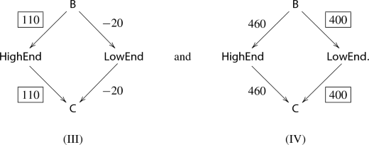
Equilibrium (III) is the equilibrium with lowest prices (and is in particular buyer-optimal), while equilibrium (IV) is the equilibrium with highest prices (and is in particular seller-optimal). Note that the high-end property is traded in equilibrium (III) while the low-end property is traded in equilibrium (IV).
It might be the case that both trades generate the same social surplus—but when utility were transferable, the builder and the consumer would agree on this fact.
These results are typically called Rural Hospitals Theorems because they imply that clearinghouses cannot improve the recruitment total of rural hospitals—which are often less attractive to doctors—by switching to different (stable) market-clearing mechanisms. The first Rural Hospitals Theorems were proven by Roth (1984, 1986) for many-to-one matching with responsive preferences. Rural Hospitals Theorems were also developed for many-to-many matching (Alkan 2002; Klijn and Yazıcı 2014), many-to-one matching with contracts (Hatfield and Milgrom 2005; Hatfield and Kojima 2010), and many-to-many matching with contracts (Hatfield and Kominers 2017).
Indeed, it appears that until Hatfield, Kojima, and Kominers (2019) found an indirect argument by way of a version of Holmström’s (1979) lemma, one-sided strategy-proofness of deferred acceptance in the presence of continuously transferable utility was known only for one-to-one markets (Demange 1982; Leonard 1983; Demange and Gale 1985; Demange 1987).
Intuitively, this argument shows that the allocation \((\hat{q^{}}^{i})_{i \in I}\) must be within \(\varepsilon \) utils of maximizing the sum of agents’ values over all allocations—i.e., that the allocation is approximately efficient.

References
Abdulkadiroğlu A, Pathak PA, Roth AE (2005) The New York City high school match. Am Econ Rev 95(2):364–367
Abdulkadiroğlu A, Pathak PA, Roth AE, Sönmez T (2005) The Boston public school match. Am Econ Rev 95(2):368–371
Alkan A (2002) A class of multipartner matching markets with a strong lattice structure. Econ Theory 19(4):737–746
Baldwin E, Klemperer P (2019) Understanding preferences: “demand types”, and the existence of equilibrium with indivisibilities. Econometrica 87(3):867–932
Bontemps C, Magnac T (2017) Set identification, moment restrictions, and inference. Annu Rev Econ 9:103–129
Bresnahan TF, Reiss PC (1991) Entry and competition in concentrated markets. J Polit Econ 99(5):977–1009
Ciliberto F, Tamer E (2009) Market structure and multiple equilibria in airline markets. Econometrica 77(6):1791–1828
Crawford VP, Knoer EM (1981) Job matching with heterogeneous firms and workers. Econometrica 49(2):437–450
Demange G (1982) Strategyproofness in the assignment market game. Working paper
Demange G (1987) Nonmanipulable cores. Econometrica 55(5):1057–1074
Demange G, Gale D (1985) The strategy structure of two-sided matching markets. Econometrica 53(4):873–888
Dubins LE, Freedman DA (1981) Machiavelli and the Gale–Shapley algorithm. Am Math Mon 88(7):485–494
Fleiner T, Jankó Z, Tamura A, Teytelboym A (2018) Trading networks with bilateral contracts. Working paper
Fleiner T, Jagadeesan R, Jankó Z, Teytelboym A (2019) Trading networks with frictions. Econometrica 87(5):1633–1661
Gale D, Shapley LS (1962) College admissions and the stability of marriage. Am Math Mon 69(1):9–15
Galichon A, Henry M (2011) Set identification in models with multiple equilibria. Rev Econ Stud 78(4):1264–1298
Gul F, Stacchetti E (1999) Walrasian equilibrium with gross substitutes. J Econ Theory 87(1):95–124
Gul F, Stacchetti E (2000) The English auction with differentiated commodities. J Econ Theory 92(1):66–95
Hatfield JW, Kojima F (2010) Substitutes and stability for matching with contracts. J Econ Theory 145(5):1704–1723
Hatfield JW, Kominers SD (2012) Matching in networks with bilateral contracts. Am Econ J Microecon 4(1):176–208
Hatfield JW, Kominers SD (2017) Contract design and stability in many-to-many matching. Games Econ Behav 101:78–97
Hatfield JW, Kominers SD (2019) Hidden substitutes. Working paper
Hatfield JW, Milgrom PR (2005) Matching with contracts. Am Econ Rev 95(4):913–935
Hatfield JW, Kominers SD, Nichifor A, Ostrovsky M, Westkamp A (2013) Stability and competitive equilibrium in trading networks. J Polit Econ 121(5):966–1005
Hatfield JW, Kojima F, Kominers SD (2019) Strategy-proofness, investment efficiency, and marginal returns: an equivalence. Becker Friedman Institute for Research in Economics Working Paper
Hatfield JW, Kominers SD, Nichifor A, Ostrovsky M, Westkamp A (2019) Full substitutability. Theor Econ 14(4):1535–1590
Holmström B (1979) Groves’ scheme on restricted domains. Econometrica 47(5):1137–1144
Jagadeesan R, Kominers SD, Rheingans-Yoo R (2018) Strategy-proofness of worker-optimal matching with continuously transferable utility. Games Econ Behav 108:287–294
Kelso AS, Crawford VP (1982) Job matching, coalition formation, and gross substitutes. Econometrica 50(6):1483–1504
Klaus B, Klijn F (2010) Smith and Rawls share a room: stability and medians. Soc Choice Welf 35(4):647–667
Klijn F, Yazıcı A (2014) A many-to-many ‘rural hospital theorem’. J Math Econ 54:63–73
Leonard HB (1983) Elicitation of honest preferences for the assignment of individuals to positions. J Polit Econ 91(3):461–479
Mas-Colell A, Whinston MD, Green JR (1995) Microeconomic Theory. Oxford University Press, Oxford
McVitie DG, Wilson LB (1970) Stable marriage assignment for unequal sets. BIT Numer Math 10(3):295–309
Milgrom P, Strulovici B (2009) Substitute goods, auctions, and equilibrium. J Econ Theory 144(1):212–247
Pakes A (2010) Alternative models for moment inequalities. Econometrica 78(6):1783–1822
Pakes A, Porter J, Ho K, Ishii J (2015) Moment inequalities and their application. Econometrica 83(1):315–334
Pathak PA, Sönmez T (2008) Leveling the playing field: sincere and sophisticated players in the Boston mechanism. Am Econ Rev 98(4):1636–1652
Roth AE (1982) The economics of matching: stability and incentives. Math Oper Res 7(4):617–628
Roth AE (1984) The evolution of the labor market for medical interns and residents: a case study in game theory. J Polit Econ 92(6):991–1016
Roth AE (1986) On the allocation of residents to rural hospitals: a general property of two-sided matching markets. Econometrica 54(2):425–427
Roth AE, Peranson E (1999) The redesign of the matching market for American physicians: some engineering aspects of economic design. Am Econ Rev 89(4):748–780
Schlegel JC (2016) Virtual demand and stable mechanisms. Working paper
Shapley LS (1964) Values of large games-VII: a general exchange economy with money. Memorandum RM-4248-PR, RAND Corporation
Sun N, Yang Z (2006) Equilibria and indivisibilities: gross substitutes and complements. Econometrica 74(5):1385–1402
Sun N, Yang Z (2009) A double-track adjustment process for discrete markets with substitutes and complements. Econometrica 77(3):933–952
Tamer E (2003) Incomplete simultaneous discrete response model with multiple equilibria. Rev Econ Stud 70(1):147–165
Acknowledgements
The authors thank Mohammad Akbarpour, John William Hatfield, Bettina Klaus, Shengwu Li, Paul Milgrom, Robbie Minton, Casey Mulligan, Alvin E. Roth, Alexander Teytelboym, the editor, Marc Fleurbaey, and the anonymous referee for helpful comments.
Author information
Authors and Affiliations
Corresponding author
Additional information
Publisher's Note
Springer Nature remains neutral with regard to jurisdictional claims in published maps and institutional affiliations.
This paper was previously circulated under the more amusing title “If You’re Happy and You Know It, Then You’re Matched.” This research was conducted while Jagadeesan and Rheingans-Yoo were Economic Design Fellows at the Harvard Center of Mathematical Sciences and Applications (CMSA). Jagadeesan gratefully acknowledges the support of a National Science Foundation Graduate Research Fellowship under grant DGE-1745303, as well as travel support from Harvard Business School and the Harvard Mathematics Department. Kominers gratefully acknowledges the support of National Science Foundation grant SES-1459912 and the Ng Fund and the Mathematics in Economics Research Fund of the CMSA. Jagadeesan and Kominers both gratefully acknowledge the support of the Washington Center for Equitable Growth.
Proof of Lemma 1
Proof of Lemma 1
As \(\left[ \hat{q^{}}^{};\hat{p}_{}\right] \) is an \(\varepsilon \)-equilibrium, we have that
where the last equality holds as \(\sum _{i \in I} q^{i} = \sum _{i \in I} e^{i} = \sum _{i \in I} \hat{q^{}}^{i}.\)Footnote 13 Hence, we have that
It follows that
Grouping (7) by agents, we have that
As \(\left[ q^{};p_{}\right] \) is a \(\delta \)-equilibrium, we have that
Summing (8) and (9), we have that
Hence, \(\left[ \hat{q^{}}^{};p_{}\right] \) is a \((\delta +\varepsilon )\)-equilibrium, as claimed.
Rights and permissions
Open Access This article is licensed under a Creative Commons Attribution 4.0 International License, which permits use, sharing, adaptation, distribution and reproduction in any medium or format, as long as you give appropriate credit to the original author(s) and the source, provide a link to the Creative Commons licence, and indicate if changes were made. The images or other third party material in this article are included in the article’s Creative Commons licence, unless indicated otherwise in a credit line to the material. If material is not included in the article’s Creative Commons licence and your intended use is not permitted by statutory regulation or exceeds the permitted use, you will need to obtain permission directly from the copyright holder. To view a copy of this licence, visit http://creativecommons.org/licenses/by/4.0/.
About this article

Cite this article
Jagadeesan, R., Kominers, S.D. & Rheingans-Yoo, R. Lone wolves in competitive equilibria. Soc Choice Welf 55, 215–228 (2020). https://doi.org/10.1007/s00355-019-01228-z
Received:
Accepted:
Published:
Issue Date:
DOI: https://doi.org/10.1007/s00355-019-01228-z