
Abstract
The Borda Compromise states that, if one has to choose among five popular voting rules that are not Condorcet consistent, one should always give preference to the Borda rule over the four other rules. We assess the theoretical as well as the empirical support for the Borda Compromise. We find that, despite considerable differences between the properties of the theoretical framework and the characteristics of two sets of observed ranking data, all three analyses provide considerable support for the Borda Compromise.


Notes
We describe the five voting rules in Sect. 3.
For example, Felsenthal (2012) shows that, while the Plurality rule, the Negative Plurality rule, and the Borda rule do not always elect a Condorcet winner if one exists, these rules are not vulnerable to the reinforcement paradox (which occurs when the same candidate wins in two separate electoral districts if the ballots are evaluated separately but the candidate does not win if the ballots are evaluated jointly). Felsenthal (2012) also shows that eight popular rules that always elect a Condorcet winner if one exists are nevertheless vulnerable to the reinforcement paradox.
The Impartial Anonymous Culture condition states that all possible voting situations (regardless of the value of \(k\)) are equally likely to be observed.
This is mathematically equivalent to asking each voter to submit one vote for the candidate he likes least, in which case the candidate with the fewest votes wins. Our description of the voting rule accounts for the possibility that voters feel more comfortable to vote for two candidates instead of against one candidate. Effectively, neither PR nor NPR require voters to report complete preference rankings of the candidates.
See, for example, Dodgson (1884, pp. 29–30) and Black (1958, p. 182) for concerns about obtaining complete rankings from voters. In an election with three candidates, the procedure for PER elects the same candidate as the Alternative Vote. However, the procedure for NPER does not always elect the same candidate as the Coombs rule. The Coombs rule declares a candidate as winner if this candidate is ranked first by a majority of the voters, and it eliminates candidates only if no candidate receives a majority of first-rank votes. But if such a majority-rule winner is also ranked last by the most voters, then NPER eliminates this candidate and determines the winner among the two remaining candidates.
For example, the French National Assembly uses two-stage elections for situations in which no candidate receives a majority of the votes in the first stage. In such a case, each member of the electorate is asked to cast a vote, in the second stage, for one of the candidates who received at least 12.5 % of the votes. The winner is the candidate who receives a plurality of the votes in the second round. Concerns about two-stage voting rules are raised in Condorcet (1994, pp. 174–175).
See Gehrlein and Lepelley (2012).
The appendix is available at “https://www.researchgate.net/publication/259755770_Appendix_to_A_Comparison_of_Theoretical_and_Empirical_Evaluations_of_the_Borda_Compromise?” Unlike in the two other data sets that contain thermometer scores, many voters ranked only a subset of the candidates in many of the ERS elections. Hence the ERS data have somewhat different characteristics than the two primary data sets that we analyze in this paper.
There are ways of accommodating equal ratings—for example, one can resolve ties randomly or record equal fractions of one vote for each of the tied ratings. Although we found that accommodating tied ratings in these ways made no notable difference to our results, we discarded tied responses nevertheless to avoid any suspicion that the tied ratings may have driven our results.
Determining the Condorcet efficiency for each of the five voting rules requires that we resolve any ties among the candidates consistently across rules. We achieve this by randomly choosing, for each voting situation, one of the six strict rankings as tie-breaking ranking. Whenever we encounter a tie between two or more candidates during the evaluation of a voting rule for this voting situation, we resolve the tie in favor of the candidate ranked higher (highest in case of a three-way tie) in this ranking.
Fig. 7 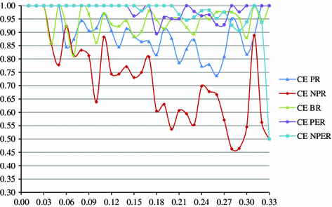
Observed ANES Condorcet efficiency values of five voting rules for parameter \(b\)
Fig. 8 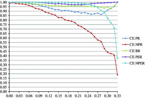
Observed PB Condorcet efficiency values of five voting rules for parameter \(b\)
We use the subscript N to distinguish \(f_\mathbf{N}\) and \(\pi _\mathbf{N} \) from other density functions and parameters vectors that we define below. Thus the subscript N is a label, and it does not denote a variable.
The voting situation of a two-candidate election consists of a vector r of length 2, and the associated density function \(f_\mathbf{P} (\mathbf{p},\pi _\mathbf{P} )\) is defined on the unit 1-simplex—a line from (0,1) to (1,0). In an election with \(n\) candidates, the density function \(f_\mathbf{P} (\mathbf{p}, \pi _\mathbf{P} )\) is defined on the unit (\(n! - 1\))-simplex.
The parameters that we use to simulate the PB voting situations imply that \(f_\mathbf{N} (\mathbf{r},\pi _\mathbf{N} )\) is the density function of the multinomial distribution, for which the limiting frequency of voting cycles equals zero. In contrast, the parameters of the ANES model imply that \(f_\mathbf{N} (\mathbf{r},\pi _\mathbf{N} )\) is the density function of the multinomial-Dirichlet distribution, which has a positive limiting frequency of cycles (see Tideman and Plassmann 2013). Thus it is not surprising that we observe a positive number of cycles in the simulated voting situations that correspond to the ANES voting situations and no cycles in the simulated voting situations that correspond to the PB voting situations.


References
Black D (1958) The theory of committees and elections. Cambridge University Press, Cambridge
Chamberlin JR, Featherston F (1986) Selecting a voting system. J Politics 48:347–369
de Condorcet M (1994) On the form of elections (1789). In: McLean I, Hewitt F (eds) Condorcet: foundations of social choice and political theory. Edward Elgar Press, Hants, pp 169–189
Daunou PCF (1991) A paper on elections by ballot (1803). In: Sommerlad F, McLean I (eds) The Political Theory of Condorcet II, University of Oxford Working Paper, pp 235–279
Dodgson CL (1884) The principles of parliamentary representation. Harrison and Sons Publishers, London
Felsenthal DS (2012) Review of paradoxes afflicting procedures for electing a single candidate. In: Felsenthal D, Machover M (eds) Electoral systems: paradoxes, assumptions, and procedures. Springer, Berlin, pp 19–91
Felsenthal DS, Machover M (1992) After two centuries, should Condorcet’s voting procedure be implemented? Behav Sci 37:250–274
Felsenthal DS, Machover M (1995) Who ought to be elected and who is actually elected? An empirical investigation of 92 elections under three procedures. Elect Stud 14:145–169
Fishburn PC (1974) Paradoxes of voting. Am Polit Sci Rev 68:537–546
Gehrlein WV (2006) Condorcet’s paradox. Springer, Berlin
Gehrlein WV (2011) Strong measures of group coherence and the probability that a pairwise majority rule exists. Qual Quant 45:365–374
Gehrlein WV, Lepelley D (2010) Voting paradoxes and group coherence: the Condorcet efficiency of voting rules. Springer, Berlin
Gehrlein WV, Lepelley D (2012) The value of research based on simple assumptions about voters’ preferences. In: Felsenthal D, Machover M (eds) Electoral systems: paradoxes, assumptions, and procedures. Springer, Berlin, pp 173–200
Plassmann F, Tideman TN (2011) How to predict the frequency of voting events in actual elections. http://papers.ssrn.com/sol3/papers.cfm?abstract_id=1911286. Mimeo
Plassmann F, Tideman TN (2014) How frequently do different voting rules encounter voting paradoxes in three-candidate elections? Soc Choice Welf 42:31–75
Regenwetter M, Grofman B, Marley A, Tsetlin I (2006) Behavioral social choice. Cambridge University Press, Cambridge
Saari DG (2001) Decisions and elections: explaining the unexpected. Cambridge University Press, Cambridge
Tideman TN, Plassmann F (2012) Modeling the outcomes of vote-casting in actual elections. In: Felsenthal D, Machover M (eds) Electoral systems: paradoxes, assumptions, and procedures. Springer, Berlin, pp 217–251
Tideman TN, Plassmann F (2013) Developing the aggregate empirical side of computational social choice. Ann Math Artif Intell 68:31–64
Author information
Authors and Affiliations
Corresponding author
Additional information
We thank Dominique Lepelley for helpful discussions and suggestions. Suggestions from two anonymous referees were very helpful in revising an earlier version of this paper.
Electronic supplementary material
Below is the link to the electronic supplementary material.
Appendix: Description of the two data sets
Appendix: Description of the two data sets
1.1 The ANES data
The ANES data contain information from the 19 time-series surveys that were undertaken by the American National Election Studies between 1970 and 2008. Survey respondents are asked to evaluate political candidates, on a “thermometer” scale from 0 to 100. In the surveys conducted before 1970, a candidate whom the survey respondent did not know received a score of 50 on the participant’s answer sheet, while such a candidate was coded as “unknown” in the surveys from 1970 onwards. To avoid ambiguities between unknown candidates and candidates evaluated at 50, we restrict our analysis to surveys conducted from 1970 onwards. ANES undertook 18 bi-annual time series surveys between 1970 and 2004 and another time series survey in 2008; ANES did not undertake time series surveys in 2006 and 2010. All possible three-candidate combinations have between 450 and 2,521 voters each. After discarding all ballots in which two or more candidates were tied, we assembled a total of 1,078 three-candidate elections with a mean of 844.9 voters.
1.2 The PB data
The PB data contain information from Politbarometer surveys that were administered by the German Institute for Election Research between 1977 and 2008. These surveys are undertaken each month, and for the years from 1990 onwards there are separate surveys for the areas of former East and West Germany. Survey respondents are asked to evaluate political candidates as well as political parties, on an 11-point “thermometer” scale from \(-5\) to +5. We consider only the thermometer scores for the political candidates and ignore the evaluations of political parties. While there are many ways in which one can combine these surveys, we decided to keep them in the format in which they are available online at the GESIS-Leibniz-Institute for the Social Sciences: combine the monthly surveys to obtain an annual survey and keep the separate surveys for East and West Germany, for a total of 49 different “elections.” Our main rationale for this decision was that assembling all three-candidate combinations within each election yields a set of elections whose numbers of voters are comparable to those in the ANES data set. Compiling all combinations of three candidates leads to a total of 83,701 three-candidate elections with between 155 and 3,934 voters and with a mean of 883.8 voters. When we eliminate those ballots on which two or more candidates are tied, we are left with 82,919 three-candidate elections with a mean of 496.7 voters.
Rights and permissions
About this article
Cite this article
Gehrlein, W.V., Plassmann, F. A comparison of theoretical and empirical evaluations of the Borda Compromise. Soc Choice Welf 43, 747–772 (2014). https://doi.org/10.1007/s00355-014-0798-7
Received:
Accepted:
Published:
Issue Date:
DOI: https://doi.org/10.1007/s00355-014-0798-7