An imaging technique for determining the volume fraction of two-component droplets of immiscible fluids

Abstract

Droplets within droplets occur in numerous situations in which two immiscible liquids interact, for instance, binary drop collisions or when a drop of one liquid impacts onto a film of a different liquid, ejecting secondary droplets containing both liquids. In the present study, an imaging technique for determining the volume fraction of each liquid component in such two-component droplets is introduced, in which multiple images of the same droplet at different times are used. The processing of these images is supported by a machine learning algorithm, which is taught using synthetically generated images and validated on droplets with known mixture fractions placed in an acoustic levitator. The application of the technique is demonstrated by measuring the volume fraction in splashed secondary droplets following the impact of a drop of one liquid onto a film of a different liquid.

Graphical abstract

1 Introduction

The impact of a single drop onto a liquid film can result in different outcomes such as deposition, formation of a corona without splash, partial rebound and splash. This study focuses on situations where the drop impact results in a splash. Whether or not a drop impact results in a splash depends on many different parameters the most important of which are the Reynolds (Re) and Weber (We) numbers and the dimensionless film thickness (Yarin et al. 2017; Moreira et al. 2010).

The critical threshold above which splashing occurs can be described by the K-number in the form $K=\text {We}^a\text {Re}^b$, first introduced by Mundo et al. (1995). Liang and Mudawar (2016) summarize numerous semi-empirical correlations which have been developed to describe the splashing threshold in this form.

The case in which the drop and film liquid differ in their essential parameters of density, viscosity and surface tension is particularly relevant to exhaust gas after-treatment systems and internal combustion engines.

Due to the ever-smaller engines, the understanding of the drop/spray wall interaction is becoming increasingly important, since secondary droplets resulting from drops impacting the oil film on the cylinder and piston wall can transport oil into the combustion chamber and thus influence the mixture composition, potentially leading to pre-ignition and/or knocking (Kubach et al. 2018). One example of a drop impact with differing liquids is shown in Fig. 1, in which a red-dyed water drop has impacted onto a film of transparent silicone oil. It can be observed that two-component droplets are ejected from the tips of the finger jets. The entire splash event can be viewed as a high speed video in Film 1 of the supplementary material.

In situations of drop impact with drops and film being of different liquids, one measurement quantity of interest is the volume fraction of one liquid in the other. This problem has not been widely studied; more emphasis has been placed on the influence of differing liquids on the splash threshold or the hydrodynamics of crown evolution (Kittel et al. 2018; Geppert et al. 2016, 2017; Chen et al. 2017).

Optical methods are preferable for such a volume fraction measurement because of their non-intrusiveness. For instance, the addition of a fluorescent dye in the impacting drop could be considered, in which case the intensity of emitted light at the fluorescent wavelength would be proportional to the amount of liquid in the two-component droplet, that originated from the impacting drop. However, the illumination would have to be appropriate to ensure that all dye molecules in the droplet were uniformly excited, the total volume of the droplet would still have to be determined, and internal absorption and secondary scattering would have to be accounted for, as with other quantitative applications of laser-induced fluorescence (Greszik et al. 2011). Optical techniques using elastic light scattering could also be considered. Although analytical solutions for the light scattering from a sphere with an eccentrically located spherical inclusion have been presented (Gouesbet and Gréhan 2000; Videen et al. 1995; Borghese et al. 1992; Fuller 1995; Wang et al. 2011; Cui and Han 2014), these analyses have yet to lead to instruments capable of quantifying the inclusion volume. Given that no technique is presently available for this measurement task, the present study introduces a chromatic, high-speed imaging approach, employing two simultaneous imaging perspectives to estimate the embedded volume fraction.

The method presented is applicable beyond the context of drop impact. The handling of two-component droplets is of growing importance for the development and designs of miniaturized microfluidic devices, with applications in the food or pharmaceutical industry (Blanken et al. 2021). An example of an application already made possible by a better understanding of the behavior of composite droplets is high throughput biological assays (Mary et al. 2011) .

Fig. 1

a Snapshot of a red-colored water droplet ($D =$ 3 mm, $u=3.2$ m/s) impinging onto a film of silicone oil ($\nu =10 \times 10^{-6}$ m$^2$s$^{-1}$) of 600 μm thickness, illustrating the generated secondary droplets; b, c Time sequence of secondary droplets ejected from finger jets

2 Problem description

Quantification of the volume fraction of two-component droplets is challenging, because the orientation of the droplet with respect to the illumination and/or imaging optics is not known a priori and also changes with time. For instance, Fig. 2 shows a red-colored water droplet encapsulated in silicone oil suspended in an acoustic levitator at consecutive time steps. While at t = 0.232 s, the projected part of the inner droplet only covers a small portion of the total projected area, at t = 0.6 s, it occupies almost the entire area. The size of the projected image of the encapsulated droplet varies depending on its position in the outer droplet relative to the observer.

Fig. 2

Levitated two-component droplet ($V_\text {frac}=0.13$) of red colored water and silicone oil ($\nu =20 \times 10^{-6}$ m$^2$s$^{-1}$) for various time instances

To quantitatively determine the size of the projected area of the inner droplet, an elementary ray-tracing approach was employed, as illustrated in Fig. 3a. Assuming the inner droplet is sufficiently illuminated, light emanating from the inner (colored) droplet will reach the observer (positioned at $y=-\infty$) after being refracted once at the outer droplet/gas interface. By examining all rays coming from the observation direction that intersect the droplet, Snell’s law is applied at the gas/droplet interface to determine whether the ray will emanate from the inner droplet or not. This we term ’inverse ray-tracing’. For this, the refractive index of the gas, $n_0$ and that of the liquid droplet n must be known. Thus, the black rays in Fig. 3a will not image the inner, colored droplet and the projected image, here in the X-Z plane, will appear as shown in Fig. 3b. This approach neglects rays with two or more internal reflections before reaching the observer, but in a similar study, such secondary reflections were shown to be negligible (Frackowiak and Tropea 2010), making a more complex ray-tracing routine unnecessary.

Fig. 3

a Schematic representation of ray paths refracted in a two-component droplet in a sectional view. b projected image from a viewer’s perspective. c definition of coordinate system origin. d definition of projected eccentricity vector

The ratio of projected areas from the inner to outer droplet can be expressed as

$$\begin{aligned} A_\text {ratio}=\frac{A_\text {inner}}{A_\text {total}}. \end{aligned}$$

(1)

The relative position of the inner droplet has a strong influence on the shape and size of the projected area of the inner droplet on the image. In order to describe the position explicitly, a coordinate system located in the center of the two-component droplet is introduced in Fig. 3c. The position of the inner droplet is denoted by the eccentricity $e_i$ describing the normalized vector between the center of mass of the inner droplet and that of the outer droplet:

$$\begin{aligned} e_x=\frac{x}{D_\text {maj}/2},\quad e_y=\frac{y}{D_\text {maj}/2},\quad e_z=\frac{z}{D_\text {min}/2}. \end{aligned}$$

(2)

where (x, y, z) describes the position of the center of the inner droplet, and $D_\text {min}$ and $D_\text {max}$ are the directional associated half-axes of the ellipsoidal-shaped droplet. The eccentricity vector $e_i$ is not directly observable from the experiments since the projected images of the inner droplet are distorted due to refraction. In order to be able to estimate the position of the inner droplet, the normalized projected eccentricity $e_{i,\text {proj}}$ is introduced, describing the vector between the centers of the two projected areas, outer to inner droplet (see Fig. 3d). Since the shape of the projected image is also influenced by the local curvature of the outer droplet, and thus, by the deformation of the entire droplet, the ellipsoidal deformation $\varepsilon$ is introduced

$$\begin{aligned} \varepsilon = \frac{D_\text {min}}{D_\text {maj}}. \end{aligned}$$

(3)

A ray-tracing approach was used to provide quantitative insight into how different parameters influence the projected area ratio and eccentricity and how these relate to the volume fraction $V_\text {frac}$, defined by

$$\begin{aligned} V_\text {frac}=\frac{V_\text {inner}}{V_\text {outer}} \end{aligned}$$

(4)

whereby $V_\text {outer}$ includes the inner volume.

A comparison between an actual two-component droplet and a corresponding synthetic image is displayed in Fig. 4. In the figure, the known volume fraction of the droplet imaged in Fig. 4a was used in the ray-tracing tool, and the eccentricities of the inner drop were adjusted iteratively until the synthetic image in Fig. 4b was similar to that in Fig. 4a. The resulting area ratio and eccentricities collated very closely to those from the experiment, verifying the ray-tracing approach for simulating the light scattering from such two-component droplets.

Fig. 4

a Levitated two-component droplet of red-colored water and silicone oil ($\nu =20 \times 10^{-6}$ m$^2$s$^{-1}$), $V_\text {frac}=0.13$, $A_\text {ratio} = 0.41$, $e_\text {x,proj}=-0.21$,$e_\text {z,proj}=-0.15$, $\varepsilon = 0.68$. b Projected view on a two-component droplet modeled after (a) using ray-tracing resulting in $A_\text {ratio} = 0.41$, $e_\text {x,proj}=-0.2$, $e_\text {z,proj}=-0.17$

The influence of $V_\text {frac}$ on the projected $A_\text {ratio}$ is displayed in Fig. 5a. For this computation spherical droplets are considered for three cases with varying positions of the inner droplet in the x direction as illustrated in Fig. 5b. In the first case, the inner droplet is located on the front side facing the observer; in the second case, the inner droplet is in the center; and in the last case, the inner droplet is on the backside of the outer droplet. Three conclusions can be drawn from these results.

• The $A_\text {ratio}$ depends strongly on the $V_\text {frac}$ and $e_i$, which means that a prediction of $V_\text {frac}$ by only the $A_\text {ratio}$ is not possible unambiguously.

• There is a limit when the $A_\text {ratio}$ reaches unity, since no information about the inner droplet position can be extracted anymore and the outer droplet appears as if it is composed of only one component. The limiting $V_\text {frac}$, indicated by the dashed lines in the figure, increases the closer the inner droplet is located to the observer.

• The slope of the curves decreases the closer the inner droplet is positioned to the front side, allowing a more accurate volume fraction quantification.

Fig. 5

a Relation between $V_\text {frac}$ and $A_\text {ratio}$ in dependence of the relative position of the inner droplet (${e_y}=e_z=0$, $n/n_0 = 1.41$). Dashed lines represent the $V_\text {frac}$ for which the $A_\text {ratio} = 1$. b Light ray paths of a two-component droplet in sectional view, resulting in varying $A_\text {ratio}$

As can be seen from Fig. 5, information about the position of the inner droplet is necessary to determine $V_\text {frac}$. For this reason, a second imaging perspective, orthogonal to the first one, is added, enabling depth perception. Figure 6a shows a schematic sectional view from above, whereas Fig. 6b shows the corresponding projected images from the two perspectives. The location of the inner droplet can be estimated by considering the projected eccentricities $e_\text {i,proj}$ from both perspectives. In the present example, both projected eccentricities $e_\text {x,proj}, e_\text {y,proj}$ are on the left side of the two-component droplet center, and thus, the position of the inner droplet is in the upper left quadrant of the sectional view. Moreover, the additional information from the second projected area ratio $A_\text {ratio}$ can improve the volume fraction estimation. The further the inner droplet moves away from the center of the outer droplet, the larger are the shape and size differences on the projected images.

Fig. 6

a Schematic of a sectional view of the two-component droplet. b Corresponding projected images from two sides. The blue and red dots represent the center of mass of the two-component droplet and the projected area, respectively

3 Description of method

It becomes apparent that due to the influence of refraction inside the two-component droplet, the real position of the enclosed droplet cannot be determined unambiguously. Only the projected eccentricities $\vec {e}_{i,\text {proj}}$ can be measured directly from the recordings. This makes direct solution of the inverse problem difficult. On the other hand, the projected $A_\text {ratio}$ in combination with $\vec {e}_{i,\text {proj}}$ does include information about $V_\text {frac}$. In order to utilize this information to determine the $V_\text {frac}$, a support vector machine (SVM) is used. The SVM is a methodology from the field of machine learning, first introduced by Cortes and Vapnik (1995), which has become widely used for solving classification problems (Awad and Khanna 2015).

3.1 SVM for volume ratio determination

The aim of using a SVM in the context of this study is to provide an algorithm, which is able to predict a volume fraction ${\hat{V}}_\text {frac}$ based on experimentally observable features, summarized in an observation vector $\vec {b}$.

SVMs belong to the category of supervised learning methods, meaning that they are trained with labeled data. With the previously described ray-tracing approach, this labeled data can be easily provided because the $V_\text {frac}$ of every synthetically generated droplet image pair is known. The output size, in this case ${\hat{V}}_\text {frac}$, is divided into a fixed number of bins each of which is assigned to a specific class k. After training a decoding function $d(\vec {b})$ can be solved for every class, i.e., volume fraction bin. The class that is then predicted by the SVM based on the observation $\vec {b}$ is determined by solving the following maximization problem:

$$\begin{aligned} {{\hat{V}}_\text {frac}=\underset{k}{\text {arg max}} \ (1-|d |).} \end{aligned}$$

(5)

A detailed description of this procedure can be found in Appendix  1.

To train a SVM with the aim to predict ${\hat{V}}_\text {frac}$, first, a set of classes has to be defined. It becomes apparent from Fig. 5 that the projected $A_\text {ratio}$ is close to unity for high $V_\text {frac}$ even if the inner droplet is positioned on the side facing the observer. The $V_\text {frac}$ of cases with $A_\text {ratio}\approx 1$ cannot be determined unambiguously, since the projected image of the droplet contains limited information. A reasonable tradeoff is to limit the measuring range of $V_\text {frac}$ between 0 and 0.5. This measuring range is then divided into equal bin sizes of 0.025 resulting in 21 discrete classes each representing 5% intervals of the upper measuring range limit.

In Sect. 2, it is shown that the projected $A_\text {ratio}$ depends on $V_{\textbf {frac}}$, the refractive index n, the relative position $e_{i}$ of the inner drop and the aspect ratio $\varepsilon$ of the two-component drop. With the aim to determine $V_\text {frac}$, the information of $A_\text {ratio}$, n, $\varepsilon$ and $e_i$ must therefore be taken into account. Since it is not possible to directly determine the exact position of the inner droplet from the recordings, its position is estimated by considering the center of the projected area of the inner droplet in each perspective image $e_{i,\text {proj}}$, with $e_{i,\text {proj}}$ being a two-dimensional vector as depicted in Fig. 3d. The SVM is trained for a fixed $n=1.41$ of silicone oil, and thus, the observation vector $\vec {b}$ becomes

$$\begin{aligned} \vec {b}=[&\varepsilon , A_{\text {ratio},1}, A_{\text {ratio},2},\nonumber \\&e_{x,\text {proj},1}, e_{z,\text {proj},1}, e_{y,\text {proj},2}, e_{z,\text {proj},2} ]. \end{aligned}$$

(6)

The area ratios can be summarized in $A_{\text{ ratio, } \text{ p }}$ and the eccentricities in $e_{i,\text {proj},p}$, where the subscript $p\in [1,2]$ denotes the respective perspective 1 or 2 and the subscript i denotes the components of the eccentricity vector. The classification is based on these seven features.

In the next step, the algorithm needs to be trained, i.e., the hyperplanes for the l= 210 binary classifiers need to be found. For this purpose, 67500 synthetic observations $\vec {b}$ were generated. For each observation, two orthogonal projections are generated, as is illustrated in Fig. 6. The $V_\text {frac}$ and the position of the inner droplet $e_i$ are randomly varied, whereby $V_\text {frac}$ is limited to the interval [0, 0.5] and $e_i$ is constrained by the condition that the inner droplet must be wholly within the outer droplet. An image processing script based on the MATLAB image processing toolbox is then used to extract $A_{ratio,p}$, $\varepsilon$ and $e_{i,\text {proj},p}$ from the synthetically generated image pairs. These quantities are then combined in $\vec {b}$, and each observation is labeled with the $V_\text {frac}$ it was generated with.

Using the MATLAB machine learning toolbox, the SVM is then trained based on this large set of labeled data. During the training process, a K-fold cross-validation technique is applied for validation (Awad and Khanna 2015). Therefore, the training data set is divided into $K=5$ samples of equal size, whereby four samples are used for training, while one sample is used for validation. This step is repeated five times. In order to evaluate the quality of the trained SVM, a classification cost as shown in the matrix of Table 1 is used. By means of this matrix, penalties for improper classification can be defined which are then incorporated into further training.

Table 1 Improper classification cost matrix

The trained SVM can then be used to predict the volume fraction based on an observation vector $\vec {b}$. The output of the SVM contains the ${\tilde{d}}$ values for every class, as shown exemplary in Fig. 7. Following the relation in Eq. (5), the class with the maximum value of ${\tilde{d}}=1-|d |$ will be the resulting $V_\text {frac}$ estimate. Thus, ${\tilde{d}}$ can be interpreted as a measure for the likelihood that a particular class best describes the true $V_\text {ratio}$. The color shading in Fig. 7 is superfluous; however, this shading is introduced here to be consistent with later representation of data in Sect. 5.2

Fig. 7

Output of decoding function ${\tilde{d}}$ for every $V_\text {frac}$ class after classification. The chosen class with the maximum ${\tilde{d}}$ is marked with a circle

4 Validation

4.1 Validation using synthetic data

The approach described above is first validated using a large set of synthetically generated data. Each artificial droplet configuration is sorted into one of the 21 $V_\text {frac}$ classes and classified individually. The mean estimated volume fraction $\langle {\hat{V}}_\text {frac} \rangle$ and standard deviation are calculated from the sorted data. The results are displayed in Fig. 8. The red dashed line represents the theoretically correct classification result $V_\text {frac} = {\hat{V}}_\text {frac}$. Very good agreement between the mean classified volume fraction $\langle {\hat{V}}_\text {frac}\rangle$ and the actual volume fraction $V_\text {frac}$ is evident over the entire range of volume fraction. Slight deviations from the mean are apparent for $V_\text {frac} > 0.3$. Furthermore, the standard deviation increases, reaching its peak at $V_\text {frac} \approx 0.4$.

Fig. 8

Relation between labeled $V_\text {frac}$ and classified ${\hat{V}}_{\textbf {frac}}$. The red dashed line indicates perfect agreement, i.e., $V_\text {frac} = {\hat{V}}_\text {frac}$

Both deviations can be explained by the upper limit of volume ratio quantification from Fig. 5. This figure shows that inner droplets positioned at the center of the two-component droplet reach a projected area ratio $A_\text {ratio} = 1$ for volume fractions above $V_\text {frac} > 0.3$. This means that the information content decreases for larger inner droplets as they approach the center of the outer droplet, leading to an increase in standard deviation. To determine the influence of the number of bins on the prediction, two further SVMs were trained with 11 and 41 bin, respectively. The prediction error is then quantified by calculating the root-mean-square error $V_\text {RSME}$ over all predictions according to the following Eq. 7:

$$\begin{aligned} {V_{RSME}= \sqrt{\frac{1}{N}\sum _{N}(\bigl ({\hat{V}}_\text {frac}-V_\text {frac,true}\bigr )}.} \end{aligned}$$

(7)

Hereby N is the total number of predictions, and $V_\text {frac,true}$ is the true value used to generate the synthetic data. The $V_\text {frac,true}$ differs from the labeled $V_\text {frac}$ since the labeled $V_\text {frac}$ is already discretized by rounding $V_\text {frac,true}$ into the bins. In the step from 11 to 21 bins, the error reduces from $V_\text {RMSE,11} =0.0424$, to $V_\text {RMSE,21} =0.0396$, while from 21 to 41 bins, the error $V_\text {RMSE,41} =0.0392$ only reduces slightly. The segmentation into 21 bins is a compromise, since a further increase of bin number would result in a larger training effort while reducing the RMSE only marginally.

4.2 Experimental validation

4.2.1 Experimental method

The technique was experimentally validated using two-component droplets of known volume fraction placed in an acoustic levitator. Figure 9 shows the experimental set-up, comprising an acoustic levitator and an image acquisition system using two orthogonally aligned chromatic cameras (Photron SA-X2 with a Tokina Macro 100 ATX Pro lens and 14 mm spacer, GoPro Hero7 with Nikkon AF Micro 60 mm lens). The setup yields a spatial resolution of 0.186 mm/px and a framerate of 250 fps for the Photron SA-X2 and a spatial resolution of 0.0151 mm/px and framerate of 240fps for the GoPro Hero7. Illumination is provided by two LED lights (Veritas Constellation 120e). The background consists of opaque white acrylic glass. The acoustic levitator was a commercial instrument (Tec5, Steinbach am Taunus) operated at 58 kHz. The sound pressure level (SPL) was chosen as a minimum to still maintain a stable position of the droplet; hence minimizing the overall drop deformation. Further information regarding the deformation of droplets due to acoustic pressure in the levitator can be found in Yarin et al. (1998).

Injection and positioning of the droplet in the acoustic levitator are performed manually with a syringe in two steps. First, the red colored water droplet is inserted after which the silicone oil is added, forming the two-component droplet. For this experiment, a silicone oil with a kinematic viscosity of 20$\times 10^{-6}$ m$^2$s$^{-1}$ was used, labeled here as S20. The inner drop was colored using fuchsine. The surface tension of the dyed drop was measured to be 70$\pm 2$ mN/m using a DCAT 25 tensiometer (Dataphysics), indicating that the dye had no significant influence on the surface tension of the liquid.

The individual volumes of the liquid injected with the syringe are known, yielding the volume fraction. The camera images are then processed using an edge detection routine; the inner projected area $A_\text {inner}$ from the red channel of the RGB image. The projected eccentricities $e_\text {i,proj}$ and ellipsoid deformation $\varepsilon$ are calculated by applying the regionprops function of MATLAB

Fig. 9

Sketch of the setup for experimental validation of the technique in the acoustic levitator

4.2.2 Results

Experimental validation was conducted using a total of 32 individual silicon droplets, 20 of which had red-colored water droplets inside and 12 of which had solid, spherical particles ($D= 1\,$mm) inside. The results of these measurements are shown in Fig. 10, in which the 32 experiments are plotted with increasing volume fraction along the X-axis according to their identification number (ID). The uncertainty bars correspond to $\pm 1$ px on the respective image, which increase with volume fraction due to the growing influence of the diameter $V_\text {frac} = f(D^3_\text {inner}/D^3_\text {total})$.

The volume fraction ${\hat{V}}_\text {frac}$ estimated from the two images is marked by black markers. The graph shows good agreement between estimated and known values of volume fraction, particularly for $V_\text {frac}<0.3$, similar to the results obtained using synthetic data. Furthermore, the classification results for spherical particles are significantly better than the droplet-in-droplet cases, especially for larger values of $V_\text {frac}$. This may be due to an increasing deformation of larger inner droplets.

There are three main reasons why the inner droplet may deviate from the spherical shape, leading to the large disagreement shown in Fig. 10 between ground truth and measurement, especially for larger volume fractions. The first is because the outer droplet is deformed due to the pressure forces exerted by the acoustic field to levitate the droplet in earth’s gravity. This may lead to a shape distortion of the inner droplet as well. The second reason is that an inner and outer acoustic streaming is generated in the levitator, as is described in Yarin et al. (1998). Finally, the droplet levitated in the pressure node undergoes rotation and centrifugal forces will then act on the inner droplet, possibly also leading to shape distortion. Therefore, since droplet rotation normally plays an insignificant role in practical applications, e.g., in a corona splash, and furthermore, in practical situations, there is no acoustic pressure or acoustic streaming, and the results of the particle experiments should be more representative of the achievable accuracy with this method.

Fig. 10

Comparison between experimental and classification-based volume fraction $V_\text {frac}$ determination. Blue markers indicate droplet-in-droplet experiments with red-colored water inside S20 silicone oil, whereas red markers indicate spherical particles ($D = 1\,$mm) inside S20 silicone oil droplets. The black symbols correspond to the estimated volume fraction from the experimental images

5 Corona splash experiments

For a further demonstration of this method, measurements were made of secondary, two-component droplets originating from a corona splash. Since the method requires two orthogonal perspectives, a novel setup using mirrors has been employed, illustrated in Fig. 11. Referring to Fig. 11, the camera imaging chip is divided into half by employing a centrally placed prismatic mirror, observing the splash through two equally spaced side mirrors. This optical configuration enables observation with two orthogonal perspectives using a single chromatic high speed camera. Two issues when imaging from two perspectives must be considered: limited depth of field (DOF) and obscuring of the droplet of interest from other surrounding droplets in the experiment. These issues are largely avoided by restricting the observed portion of the splash to only a quarter of the spatial regime of splashing. A sketch of the side view of the experimental setup is presented in Fig. 12. The impinging drop is produced with a cannula and a micropump. It is accelerated by gravity onto the liquid film. The liquid is contained in a pool enclosed within surrounding multiple layers of PVC foil which are affixed to a sapphire glass plate. The liquid film depth is controlled by a confocal chromatic film thickness sensor confocalDT 2421 in combination with a IFS2405-1 probe from Micro Epsilon. The impact point of the drop is chosen such that it is visible near the outer edges of both observation fields of view (FOVs). This results in good visibility of the splash as well as enabling the velocity and volume of the impinging drop to be determined.

Fig. 11

Sketch of the splashing setup showing the respective fields of view (FOV), focal planes (FP) and depth of field

Fig. 12

Schematic representation of the experimental setup in a side view

The setup uses the Photron SA-X2 with the same objective, spacer and background configuration as in the levitator experiment. The framerate was 10000 fps at an f-stop of 11, and the DOF was $11\,$mm. The resolution was $0.037\,$mm/px. A typical single frame image is shown in Fig. 13, upon which the trajectories of several droplets have been superimposed. The trajectories have been obtained from frames taken before and after the frame pictured in this figure. The entire splash event captured with the split image can be viewed in Film 2 of the supplementary material.

Fig. 13

Single frame image from the experiment of an red-colored drop impinging onto a silicone oil film of $\nu =10 \times 10^{-6}$ m$^2$s$^{-1}$, $t=25$ ms after impact. The trajectories of the droplets are highlighted by colored lines, whereby matched pairs have the same color

5.1 Image processing

The secondary droplets created during the splash must be recognized in images from both observation directions. However, this causes difficulties since not all droplets are visible on both images due to the limited FOV. Furthermore, droplets can only be observed in focus within the limited depth of field. The DOF is therefore used to detect relevant droplets which are visible on both images. Those droplets are identified by a gradient based, circle finding algorithm which neglects drops that are too far out of focus. A simple PTV algorithm based on the nearest neighbor principle is then used to determine the droplets trajectories in consecutive images. The height of the droplet above the impact plane as a function of time, as well as the radius of the droplets, is then used to match droplets to one another on each of the images. To ensure comparability in the matching process, only droplets with a diameter of 10 pixels or more are considered.

The focal plane of each viewing perspective is positioned in relation to the outer edge of the FOV from the other viewing perspective. Its distance to the outer edge is exactly half of the experimentally predetermined DOF length. This results in a rectangular area in which a droplet is imaged sharply on both images, as indicated in Fig. 11. Droplets outside of this area may only be visible on one image or are blurred, due to being outside the DOF. The assignment process is understandably less prone to error with lower volume number densities of secondary droplets.

5.2 Experimental results

A typical measurement result, obtained by tracking a single two-component secondary droplet, is shown in Fig. 14. This corresponds to the droplet trajectory labeled #4 in Fig. 13. In Fig. 14, the complementary decoding function ${\tilde{d}}=1-|d |$ is expressed in color as a function of the $V_\text {frac}$ class between 0 and 0.5. The maximum value of ${\tilde{d}}$ for each image frame along the trajectory is marked with a black dot, and the volume fraction class in which the black dot lies corresponds to the most likely value of ${\hat{V}}_\text {frac}$. The figure shows a total of 74 frames, equally spaced in time and increasing along the ordinate. As can be seen from this figure, the estimated volume fraction lies between 0.15 and 0.225. The different estimated values of $V_\text {frac}$ at different trajectory positions (frames) arise because the orientation of the droplet with respect to the two observation directions changes along its trajectory.

Fig. 14

Output ${\tilde{d}}$ of the complementary decoding function for a set of 74 observations taken at equal times along the trajectory of a single two-component droplet, plotted as a function of the $N_r$ classes of ${\hat{V}}_\text {frac}$. For reasons of presentability, only every second result is shown. The maximum ${\tilde{d}}$, i.e., the most likely value of $V_\text {frac}$, is marked with a black dot for each frame

A total of 15 drop impact events were performed, resulting in a total of 95 secondary, two-component droplets being tracked from both imaging directions. For each secondary droplet, a result similar to that shown in Fig. 14 was obtained and a median value of ${\hat{V}}_\text {frac}$ was obtained by summing over all frames in which the droplet could be observed. A median value was used instead of a mean to diminish effects of outliers arising from the image processing, e.g., through out-of-focus blurring. In the case of Fig. 14, this median value results in ${\hat{V}}_\text {frac}=0.175$. A histogram of the obtained median volume fractions was then computed and is shown in Fig. 15. By far the most frequently encountered droplets are those with no embedded droplet, i.e., for ${\hat{V}}_\text {frac} = 0$. The frequency of droplet occurrences for the class at ${\hat{V}}_\text {frac} = 0.5$ must be interpreted as ${\hat{V}}_\text {frac} \ge 0.5$, since above a value of 0.5 no distinction regarding the true value can be made. This result cannot be verified, since ground truth is not known and no alternative measurement technique is available for comparison. Fig. 15 is therefore intended only as an illustration of what results can be derived from the measured values of ${\hat{V}}_\text {frac}$

Fig. 15

Histogram of ${\hat{V}}_\text {frac}$ measured from 95 two-components droplets originating from 15 drop impact events

6 Discussion and conclusion

Two further aspects concerning the accuracy of the measurements using this technique should be discussed. For one, the variance of the ${\hat{V}}_\text {frac}$ estimates from consecutive frames appears to increase with increasing values of $V_\text {frac}$. This is observable in Figs. 8 and 10. Indeed, when $A_\text {ratio}=1$, the uncertainty becomes a maximum and it is reasonable to assume that the uncertainty grows monotonically between values of $A_\text {ratio}$ between 0 and 1. The second issue is the question: to what degree does the accuracy depend on the number of image pairs captured along a droplet trajectory? For instance, if the droplet does not change its orientation or distance from the focal plane of each observation direction with time, then identical images will be obtained for each frame. This results in a large amount of data, but no new information. In such a case, one single frame would suffice to estimate $V_\text {frac}$.

To investigate these two aspects, the ray-tracing tool outlined in Sect. 2 can be used. By generating synthetic images and processing these as though they were measured images with known values of $V_\text {frac}$, the accuracy of the estimators can be investigated. This has been performed for exemplary values of $V_\text {frac}$, whereby each image pair used a random selection of $e_{i,\text {proj},p}$ values at a fixed droplet deformation of $\varepsilon = 1$. Using random values ensures that each new data set (image pair) represents also new information. The results of this exercise are shown in Fig. 16 from which the following observations can be made:

• The mean error and its deviation decrease faster for smaller values of $V_\text {frac}$. Only a few data sets (frames) are necessary for a reliable prediction if $V_\text {frac}$ is relatively small.

• There is virtually no error at $N_d = 30$ for low values of volume fraction, i.e., $V_\text {frac} < 0.15$. For larger values of $V_\text {frac}$, the uncertainty of the estimated volume fraction no longer decreases with increasing number of data sets, as evident from Figs. 16b and d.

  Fig. 16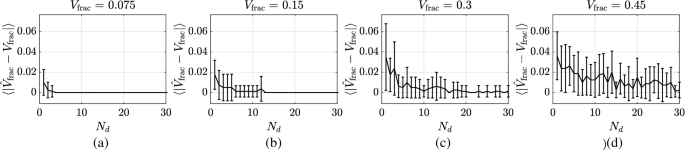

  

  Relation between the number of available data sets for classification ($N_d$) and the mean absolute error between known and estimated volume fraction $\langle \Vert {\hat{V}}_\text {frac}-V_\text {frac}\Vert \rangle$

These observations both suggest that this technique is particularly well suited for applications in which low volume fractions can be expected. In such cases, the required number of image frames is quite modest, whereby this refers to the number of independent frames, since the data in Fig. 16 were generated using random input values for the observation vector $\vec {b}$. Using a high speed camera, consecutive images would normally be highly correlated with one another; hence, they would not each be delivering totally new information as with randomly chosen $\vec {b}$ vectors. The time between frames to insure that new, uncorrelated information is obtained would depend on the integral time scale of the image pattern variations, a quantity which would be very specific to a particular application and is therefore, beyond the scope of the present study.

Nevertheless, the fact that reliable ${\hat{V}}_\text {frac}$ estimates can be made with only few image pairs suggests that shorter segments of the droplet trajectory can be used for processing, for instance, by restricting the SVM procedure to images with much less out-of-focus blur. This would also decrease the number of outliers in the estimation procedure and is one of the planned refinements of the present study.

Another field of future study is the application of this technique to examine droplets with embedded solid particles. Such situations arise in encapsulation processes, when solid particles are encapsulated by spraying an atomized liquid into a fluidized bed of particles. After some period, the outer liquid shell solidifies and encapsulates the inner particle, a process common in the pharmaceutical industry. Application of this technique would of course necessitate a clear difference in color between the solid particle and the surrounding liquid.

The situation of solid particles embedded in an outer liquid droplet also offers an interesting alternative method of validating the measurement technique. If monodispersed particles were used, then the volume fraction would always be known, once the outer drop diameter was determined. This known value could then be compared with the measured value. This would complement the validation presented here using the acoustic levitator.

In conclusion, a novel imaging technique for measuring the volume fraction of two-component droplets has been introduced and shown to be reliable for low values of volume fraction. The technique has been validated using droplets with known volume fraction placed in an acoustic levitator and demonstrated in practice with the example of secondary droplets emanating from the corona splash of a drop impinging onto a film of a different liquid.

Appendix A Support Vector Machine

To apply a SVM to a specific problem it first needs to be trained. The training data have n features and each data point is labeled to a specific class. The learning process can be interpreted geometrically by assigning each feature to an individual axis and plotting each data point into the feature space. The SVM then finds the optimal n-dimensional hyperplane which separates the classes from each other. In Fig. 17, a simplistic example of classification into two classes based on two features is given.

Fig. 17

Simplified example of the classification principle of an SVM after Richter (2019). The solid line shows the optimal hyperplane, the dashed lines show the optimal margin, and the support vectors are marked with black circles

The solid line describes the optimal separating hyperplane, while the dashed lines describe the margin between the classes. The margin is defined by support vectors which are marked by the dashed circles in the figure.

In case the data are not perfectly separable (Cortes and Vapnik 1995) introduced the soft margin SVM, which tolerates a certain amount of data inside the region of the margin. A further method to increase the applicability of SVMs is the use of kernel functions (Boser et al. 1992). If the data are not separable by linear hyperplanes, the n-dimensional feature space can be transformed into a higher dimensionality N and be separated by a N-dimensional hyperplane. In this way, it is possible to create arbitrary hypersurfaces to separate the patterns of classes. A detailed description of the optimization problem can be found in Awad and Khanna (2015); Cortes and Vapnik (1995); Steinwart and Christmann (2008); Bhavsar and Panchal (2012).

The result of the training process is a classifier $f_j(\vec {b})$, whereby the observation $\vec {b}$ is a vector assigned with values of the observed features. This classifier can then perform a prediction, whether the observation $\vec {b}$ belongs to class 1 or class 2. The geometrical interpretation of the process would be to plot $\vec {b}$ into the feature space and depending on which side of the hyperplane it is on, it is assigned to either class 1 or class 2. SVMs in general are binary classifiers and well suited to discriminate two classes against each other. In order to solve a multi-class problem, as in the present case, more advanced strategies such as the error correcting output (ECOC) framework, first introduced by Dietrich and Bakiri (1995), need to be applied. This framework allows for a separation of the multi-class problem into multiple binary classification problems. Basically, the ECOC method consists of a encoding step that assigns which classes of which binary classifier are to be compared, and a decoding step where the outputs of all the binary classifiers are evaluated and a predicted class is assigned Escalera et al. 2010; Allawein et al. 2000).

Two of the most prominent strategies to encode in ECOC is the one-versus-all (OVA) and the one-versus-one (OVO) method. If c is the total number of classes, in the OVA method, a number of $l=c$ binary classifiers are trained, distinguishing between one individual class and the set of all other classes. Whereas in the OVO method, a number of $l=c(c-1)/2$ classifiers are trained, building classifiers for every possible class pair (Awad and Khanna 2015; Chaitra and Saravana Kumar 2018). Which binary classifier discriminates between which classes is specified in the coding matrix $m_{kj}$, which has the dimension $i\times l$ and for whose elements the following applies: $m_{kj} \in \{1, 0, -1 \} (k \in \{1..c\}, j\in \{1..l\})$. In following Table 2, an example for a coding matrix for classification into three classes organized according to the OVO method is given. The value 1 can be translated with “class to compare,” 0 with “class to ignore” and -1 with “class to compare to” (Allawein et al. 2000). The columns define which classes are compared with each other in the respective classifier. In this example, the classifier $f_1$ discriminates between class 1 and class 2 while ignoring class 3 as defined in the first column of the coding matrix.

Table 2 Coding matrix $m_{kj}$ for a three class problem organized according to the OVO method

Each binary classifier $f_j(\vec {b})$ has an output $s_j\in \{1,-1\}$, indicating the outcome of the binary decision. According to the coding matrix in Table 2, the output of $f_1$ would be $s_1=1$ if the observation $\vec {b}$ is assigned to class 1 and $s_1=-1$ if $\vec {b}$ is assigned to class 2.

In order to infer a predicted class from the output information $s_j$ of the individual classifiers, a decoding step is necessary. The predicted class ${\hat{k}}$ is chosen by searching for the class k where the decoding function $d(m_{kj}, f_j(\vec {b})=s_j)$ is minimal for a given input observation.

$$\begin{aligned} {\hat{k}}=\underset{k}{\text {arg min}}\ d(m_{kj},s_j) \end{aligned}$$

(8)

In this study, a loss-weighted decoding following (Escalera et al. 2010) is applied resulting in the following decoding function:

$$\begin{aligned} d =\frac{\sum _{j=1}^{l} |m_{kj} |g( m_{kj} , s_j ) }{\sum _{j=1}^{l} |m_{kj} |}. \end{aligned}$$

(9)

with $g(m_{kj},s_j)$ being the loss function for which in this study the “hamming” principle has been chosen.

$$\begin{aligned} g(m_{kj},s_j)=\frac{1-sign(m_{kj}s_j)}{2} \end{aligned}$$

(10)

The output of the decoding function is a measure of how often the binary decisions based on an observation turn out in favor of a specific class. In the limiting case, d becomes 0 if every decision is in favor of the class, or d = 1 if no decision is in favor of the class. The decoding step can alternatively be expressed as a maximization problem by using the complement of the decoding function ${\tilde{d}}=1-|d |$ and the classification applies as

$$\begin{aligned} {\hat{k}}=\underset{k}{\text {arg max}} \ (1-|d |). \end{aligned}$$

(11)

This complementary approach is used in the presented study.

References

Allawein EL, Schapire RE, Singer Y (2000) Reducing multiclass to binary: a unifying approach for margin classifiers. J Mach Learn Res 1:113–141. https://doi.org/10.1162/15324430152733133
Awad M, Khanna R (2015) Efficient Learning Machines: Theories, Concepts, and Applications for Engineers and System Designers, 1st edn. Apress, Berkeley, CA
Bhavsar H, Panchal MH (2012) A review on support vector machine for data classification. Int J Adv Res Comput Eng Technol 1:185–189
Blanken N, Saleem MS, Thoraval M et al (2021) Impact of compound drops: a perspective. Curr Opin Colloid Interface Sci. https://doi.org/10.1016/j.cocis.2020.09.002
Borghese F, Denti P, Saija R et al (1992) Optical properties of spheres containing a spherical eccentric inclusion. JOSA A 9(8):1327–1335. https://doi.org/10.1364/JOSAA.9.001327
Boser BE, Guyon IM, Vapnik VN (1992) A training algorithm for optimal margin classifiers. In: Proceedings of the fifth annual workshop on computational learning theory, pp 144–152. https://doi.org/10.1145/130385.130401
Chaitra PC, Saravana Kumar R (2018) A review of multi-class classification algorhythms. Int J Pure Appl Math 118:17–26
Chen N, Chen H, Amirfazli A (2017) Drop impact onto a thin film: miscibility effect. Phys Fluids 29(9):092106. https://doi.org/10.1063/1.5001743
Cortes C, Vapnik V (1995) Support-vector networks. Mach Learn 20:273–297. https://doi.org/10.1007/BF00994018
Cui Z, Han Y (2014) A review of the numerical investigation on the scattering of gaussian beam by complex particles. Phys Rep 538(2):39–75. https://doi.org/10.1016/j.physrep.2014.01.002
Dietrich TG, Bakiri G (1995) Solving multiclass learning problems via error-correcting output codes. J Artif Intell Res 2:263–286. https://doi.org/10.1613/jair.105
Escalera S, Pujiol O, Radeva P (2010) On the decoding process in ternary error-correcting output codes. IEEE Trans Pattern Anal Mach Intell 32:120–134. https://doi.org/10.1109/TPAMI.2008.266
Frackowiak B, Tropea C (2010) Numerical analysis of diameter influence on droplet fluorescence. Appl Opt 49(12):2363–2370. https://doi.org/10.1364/AO.49.002363
Fuller KA (1995) Scattering and absorption cross sections of compounded spheres. III. Spheres containing arbitrarily located spherical inhomogeneities. JOSA A 12(5):893–904. https://doi.org/10.1364/JOSAA.12.000893
Geppert A, Chatzianagnostou D, Meister C et al (2016) Classification of impact morphology and splashing/deposition limit for n-hexadecane. Atomization Sprays. https://doi.org/10.1615/AtomizSpr.2015013352
Geppert A, Terzis A, Lamanna G et al (2017) A benchmark study for the crown-type splashing dynamics of one-and two-component droplet wall-film interactions. Exp Fluids 58(12):172. https://doi.org/10.1007/s00348-017-2447-2
Gouesbet G, Gréhan G (2000) Generalized Lorenz-Mie theory for a sphere with an eccentrically located spherical inclusion. J Mod Opt 47(5):821–837. https://doi.org/10.1080/09500340008235093
Greszik D, Yang H, Dreier T et al (2011) Laser-based diagnostics for the measurement of liquid water film thickness. Appl Opt 50(4):A60–A67. https://doi.org/10.1364/AO.50.000A60
Kittel HM, Roisman IV, Tropea C (2018) Splash of a drop impacting onto a solid substrate wetted by a thin film of another liquid. Phys Rev Fluids 3(7):073601. https://doi.org/10.1103/PhysRevFluids.3.073601
Kubach H, Weidenlener A, Pfeil J et al (2018) Investigations on the influence of fuel oil film interaction on pre-ignition events in highly boosted di gasoline engines. Tech. rep., SAE Technical Paper. https://doi.org/10.4271/2018-01-1454
Liang G, Mudawar I (2016) Review of mass and momentum interactions during drop impact on a liquid film. Int J Heat Mass Transf 101:577–599. https://doi.org/10.1016/j.ijheatmasstransfer.2016.05.062
Mary P, Chen A, Chen I et al (2011) On-chip background noise reduction for cell-based assays in droplets. Lab Chip 11:2066. https://doi.org/10.1039/C1LC20159J
Moreira A, Moita A, Panao M (2010) Advances and challenges in explaining fuel spray impingement: how much of single droplet impact research is useful? Prog Energy Combust Sci 36(5):554–580. https://doi.org/10.1016/j.pecs.2010.01.002
Mundo C, Sommerfeld M, Tropea C (1995) Droplet-wall collisions: experimental studies on the deformation and breakup process. Int J Multiph Flow 21:151–173. https://doi.org/10.1016/0301-9322(94)00069-V
Richter S (2019) Statistisches und maschinelles lernen: Gängige verfahren im überblick. Springer, Berlin, Heidelberg
Steinwart I, Christmann A (2008) Support vector machines, 1st edn. Information Science and Statistics, New York, NY. https://doi.org/10.1007/978-0-387-77242-4
Stumpf B, Rüsch JH, Roisman IV et al (2022) Supplementary material. https://doi.org/10.48328/tudatalib-831
Videen G, Ngo D, Chỳlek P et al (1995) Light scattering from a sphere with an irregular inclusion. JOSA A 12(5):922–928. https://doi.org/10.1364/JOSAA.12.000922
Wang J, Gouesbet G, Han Y et al (2011) Study of scattering from a sphere with an eccentrically located spherical inclusion by generalized lorenz-mie theory: internal and external field distribution. JOSA A 28(1):24–39. https://doi.org/10.1364/JOSAA.28.000024
Yarin A, Pfaffenlehner M, Tropea C (1998) On the acoustic levitation of droplets. J Fluid Mech 356:65–91
Yarin AL, Roisman IV, Tropea C (2017) Collision phenomena in liquids and solids. Cambridge University Press, Cambridge
Acknowledgements
The authors gratefully acknowledge the financial support of the Deutsche Forschungsgemeinschaft (DFG) through the Project SFB/TRR 150, project number 237267381, subproject A02. Furthermore, the authors would like to thank Dr.-Ing. H. Kittel and the student group of L. M. Reitter, F. Goertz, N. M. Quernheim and R. P. Schultheis for their valuable preliminary work.
Funding
Open Access funding enabled and organized by Projekt DEAL.
Author information
Authors and Affiliations
Contributions
BS contributed to investigation, methodology, software data curation, writing—original draft; JHR contributed to methodology, software, data curation and investigation; IVR was involved in supervision, methodology ; CT contributed to conceptualization, writing, review and editing, funding acquisition; JH contributed to supervision, methodology, project administration and funding acquisition.
Corresponding author
Additional information
Publisher's Note
Springer Nature remains neutral with regard to jurisdictional claims in published maps and institutional affiliations.
Supplementary Information
Below is the link to the electronic supplementary material.
Supplementary file 1 (avi 10599 KB)
Supplementary file 2 (avi 8743 KB)