
Abstract
Competition between individuals of the same or different species affects spatial distribution of organisms at any given time. Consequently, a species geographical distribution is related to population dynamics through density-dependent processes. Small Arctic rodents are important prey species in many Arctic ecosystems. They commonly show large cyclic fluctuations in abundance offering a potential to investigate how landscape characteristics relates to density-dependent habitat selection. Based on long-term summer trapping data of the Norwegian lemming (Lemmus lemmus) in the Scandinavian Mountain tundra, we applied species distribution modeling to test if the effect of environmental variables on lemming distribution changed in relation to the lemming cycle. Lemmings were less habitat specific during the peak phase, as their distribution was only related to primary productivity. During the increase phase, however, lemming distribution was, in addition, associated with landscape characteristics such as hilly terrain and slopes that are less likely to get flooded. Lemming habitat use varied during the cycle, suggesting density-dependent changes in habitat selection that could be explained by intraspecific competition. We believe that the distribution patterns observed during the increase phase show a stronger ecological signal for habitat preference and that the less specific habitat use during the peak phase is a result of lemmings grazing themselves out of the best habitat as the population grows. Future research on lemming winter distribution would make it possible to investigate the year around strategies of habitat selection in lemmings and a better understanding of a fundamental actor in many Arctic ecosystems.
Introduction
Habitat selection is crucial for animals and the characteristics of the chosen site can determine food availability, exposure to harsh climate and predation risk, and hence directly affect survival and reproductive success (Morris 1999). However, there is often a trade-off between food availability and shelter, where the most productive areas not always offer good protection and vice versa (Brown et al. 1999). For animals living in areas with strong seasonality, such trade-off is further complicated as a good summer habitat might not be a suitable winter habitat and the individuals have to either engage in seasonal migration or cope with suboptimal conditions (Cohen 1967).
Population size can also affect habitat selection through intraspecific competition, known as density-dependent habitat selection (Morris 1989, 1999). When individuals are excluded from more suitable habitats, they have to inhabit inferior marginal habitats often associated with higher risks of predation or starvation (Errington 1946). If habitat selection is density-dependent, we would, therefore, expect individuals at low density to be more habitat specific compared to individuals in a population where competition is higher (Fretwell and Lucas 1970). This suggests that habitat selection should be studied both in the light of habitat quality and population density. When a population is small, the distribution of a species should provide a strong ecological signal regarding suitable habitat (Fretwell and Lucas 1970). Strong intraspecific competition for habitat, on the other hand, could weaken the ecological signal of habitat choice if many individuals are forced to reside in low-quality habitats. By comparing density-dependent differences in distribution, it could hence be possible to test if animals are more habitat specific when population densities are low, and if habitat selection reflects trade-offs between food, shelter, and need for seasonal migration.
Several small mammal species are known for their phenomenal cyclic fluctuations in abundance (Hansson 1971; Bjørnstad et al. 1995; Hörnfeldt 2004; Krebs 2011) and cyclic small rodents are key herbivores in tundra ecosystems at high latitudes of the northern hemisphere (Ims and Fuglei 2005). They can have a large impact on vegetation (Olofsson et al. 2012) as well as predators and indirectly also on alternative prey species (Ims and Fuglei 2005). The Norwegian lemming (Lemmus lemmus) shows spectacular cyclic fluctuations in population abundance (Elton 1924) ranging from virtually absent to super abundant in a cycle that typically last 3–5 years. Despite considerable research, the ecology of the Norwegian lemming is still unknown in many aspects (Chitty 1960; Stenseth and Ims 1993); for example, the mechanisms behind the population cycle have been debated for a long time (Chitty 1960). Regardless of the specific drivers of the population cycle, the substantial fluctuations in abundance provide an excellent study system to investigate how habitat selection could be affected by population density. However, the large fluctuations would also pose a methodological problem. Lemming distribution is almost impossible to study at the low phase, because at low density, lemmings are virtually undetectable, but during peak years, they are ubiquitous. Framstad and Stenseth (1993) found, for example, no strong habitat preference during a peak phase year. However, the distribution in moderately numerous populations during the increase phase, in the transition from low to peak abundance, is possible to study and would likely reflect habitat selection at low density. This could be compared with the less specific habitat selection expected during a peak phase when suboptimal habitats should be used to a larger extent.
Lemmings feed mainly on mosses, graminoids, and sedges (Tast 1991; Soininen et al. 2013, but see Soininen et al. 2017) and the distribution of food depends partly on snow conditions as snow have a big impact on plant distribution in the mountain tundra (Ravolainen et al. 2011) due to the long winters during which snow covers the ground (about 8 months). Snow affects the micro-climate which creates ecological niches for different plants (Ravolainen et al. 2011). For example, snow bed habitat has a high richness of plants, similar to that in locally more productive habitats (Bruun et al. 2006).
Topography is one of the main factors influencing accumulation, depth, and condition of snow (in European mountains: Anderton et al. 2004; Lopez-Moreno and Stähli 2008; in North America: Pomeroy et al. 1998; Molotch et al. 2005), and we would hence expect topography to indirectly influence food availability, and in turn lemming habitat selection. Topography would also affect the conditions for plants during and after snowmelt as concave landscape elements are expected to be generally more productive than surrounding ridges with convex topography. Concave sites have usually water and nutrient run-off along a ridge-leeside-snow bed gradient that would be expected to correspond to a plant productivity gradient (Moen 1998; Billings 2000). Topography could also affect the occurrence of shelters where lemmings could seek protection from predators and dig burrows. This can be seen, for example, along small streams that have carved gullies into the soil (Henttonen and Kaikusalo 1993). Flat areas could possibly pose a problem if they frequently get flooded, and slope steepness could hence affect the numbers of suitable burrows for lemmings. Since vegetation and snow are key factors affecting lemming, we tested the implication of these variables on the distribution of Norwegian lemmings during two phases of their cycle. We used generalized linear models (GLM) to investigate the presence/pseudo-absence estimated with snap trapping in the Scandinavian mountain tundra during the increase (n = 105 trapping plots) and peak phase (n = 151 trapping plots) of the rodent cycle, in relation to environmental variables. During the increasing phase, lemming habitat was studied at ‘trapping plot scale’ (represents about one point for 536 m2). During the peak phase, lemming habitat was also studied at ‘trapping station scale’ (represents one point for 19.7 m2; n = 588 trapping stations). In the trapping station scale, we were able to investigate plant species composition and primary productivity on a scale relevant for lemming territories. Comparing two phases of lemming cycle, we tested the general hypothesis that with increasing population density, lemmings should extend their habitat from habitat with readily available food plants and potentially good overwintering conditions to include less favourable areas. We examined here if the characteristics of their habitat used could offer them better overwintering conditions in term of food availability.
Materials and methods
Study area
This study was carried out in three areas of the Scandinavian mountain tundra (Fig. 1), in Helags, Jämtland county (≈ 62°54′N, 12°27′E), Vindelfjällen, Västerbotten county (≈ 67°00′N, 17°00′E) and Borgafjällen/Børgefjell, Västerbotten county in Sweden, and Nordland in Norway (≈ 65°00′N, 15°00′E). The Norwegian lemming is common in the study areas. Strong lemming cycles were disrupted during the 1980s and 1990s. However, according to the National Environmental Monitoring Programme (Hörnfeldt 2013), the lemming population currently follows a classical 3- to 4-year cycle.

Maps from http://www.diva-gis.org
Study areas located in Vindelfjällen (V), Borgafjällen/Børgefjell (B), and Helags (H). Black symbols represent trapping realized during peak years, whereas white ones represent trapping realized during increase year.
To determine the phase of the lemming cycle, we used trapping data from Hörnfeldt lines (see below). We calculated the average number of specimens trapped per 100 trap-nights each spring and autumn together based on all sampling plots per region (Fig. 3). The peak phase was defined as the maximum density over 3–4 years and the increase phase as the year before the peak. The increase phase was characterized by a distinct shift in rate of change in number from low to high density (see Hörnfeldt 2004 for details). The abundance of lemmings was high in 2001, 2004, 2007, and 2011 (Fig. 3). Based on the definition, we classified 2001, 2007, and 2011 as peak years and 2006 and 2010 as increase years. Too few animals were trapped in 2003, and we have no data from 2000 and 2004. We did not include data from 2004 because of the low number of trapped individuals (we did not trap any lemming on Programme 2 in Krebs lines, see below).
The data used were collected within three programs described below. Data from all programmes were used to analyse trapping plot habitat selection patterns (100–300 m resolution). However, to analyse station habitat selection (15 m resolution, Table 1), only data from one programme in one area were used (Programme 2, in Helags). We used data both on presences, i.e., when at least one individual was caught in the capture session on the entire line, square or station, and absence, i.e., when no individual was caught in the capture session on the entire line, square, or station. Several studies of distribution lack absence data and were thus forced to use presence-only modeling (Pearce and Boyce 2006) with a use of “pseudo-absence”. Here, to model the summer distribution of lemmings, we had access to both the presence and absence that we call pseudo-absence (as real true-absence is hard to achieve in the field).
The study areas include different vegetation types, such as wetland, meadow, and heath (Moen 1998). Wetlands are dominated by sedges (Carex aquatilis, Eriophorum scheuchzeri) and graminoids (Poa sp. and Pleuropogon sabinei). Mesic areas are mainly composed of forbs (Saxifraga spp., Potentilla spp., Ranunculus spp.), graminoids, shrubs (Salix spp.), and mosses. Dry heath areas are dominated by Vaccinium myrtillus, Empetrum nigrum, and lichens.
Species data
Lemming distribution and habitat selection were assessed using snap-trapping data from three different monitoring programmes. Trapping of animals has been evaluated and recurrently ethically approved by concerned authorities in all monitoring programmes (Norway: Norwegian Environment Agency (Miljødirektoratet); Sweden: Swedish board of agriculture (Jordbruksverket) and Umeå djurförsöksetiska nämnd. We used three different monitoring programs which are explained below:
-
1.
We used line transect data from the National Environmental Monitoring Programme for small rodents in Vindelfjällen and Helags in 2001–2012 (Hörnfeldt 2013). Here, we call these lines “Hörnfeldt lines”. These trappings were carried out along approx. 3 km-long altitudinal transects with 6–9 permanent 100 × 100 m trapping plots spaced at intervals of ca. 300 m along the transects (Fig. 2a; see also Hörnfeldt 2004). Each transect covered an altitudinal gradient from conifer forest to tree-line birch forest, to open habitats with heaths, meadows, fens, and snow beds. However, to homogenise our datasets, for the analysis of habitat selection, we only used data from above the tree line: 16 out of normally 44 trapping plots in Vindelfjällen (Ammarnäs), and 17 out of 42 plots in Helags (Vålådalen/Ljungdalen). 10 trap stations spaced 10 meters apart, with 5 snap traps each were distributed along the diagonal of each 1 ha trapping plot. This method corresponds to 1.59 traps for 1 m2. Trapping was carried out twice per year, in spring (late June) and autumn (mid-August). Traps were set for three nights, i.e., normally corresponding to a trapping effort of 150 trap-nights per plot and season. For further details of the trapping design and trapping methods, see Hörnfeldt (2004). Lemming captures were too rare to allow analysis in all years, but we included data from the 2 years which represented the highest amplitude cycle during the study period (Fig. 3), i.e., the increase year in 2010 (n = 33 lines) and the peak year in 2011 (n = 33 lines). Hereby, we limited confounding year and phase effect.
Fig. 2 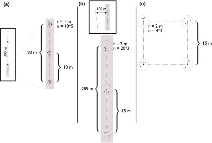
Trapping protocols of a Hörnfeldt lines; b Krebs lines; and c Myllymäki quadrates
Fig. 3 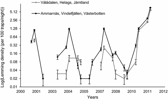
Data from Hörnfeldt (2013)
Lemming density (number of individuals trapped per 100 trap-nights) ± SE in late June and mid-August 2001–2012 in Vålådalen, Helagsfjällen (in grey; normally 42 sampling plots) and Ammarnäs, Vindelfjällen (in black; normally 44 sampling plots).
-
2.
In Vindelfjällen, Borgafjäll and Helags, small rodents were trapped along transects in mountain tundra habitat of varying types within Arctic fox territories in July 2001–2013, following the trapping protocol described by Krebs et al. (2002). Here, we called these lines “Krebs lines”. We used two (or in some cases three) parallel snap-trap lines separated by 100 m with 20 stations placed at 15-m intervals on each line. At each trap station, we placed 3 traps at favourable positions within 1–2 m from the central point (Fig. 2b; corresponding to 0.13 trap per 1 m2). Traps were set for 48 h per territory and traps were checked four times at 12-h intervals. Data from peak years in 2001 (n = 8), 2007 (n = 61) and 2011 (n = 9), as well as data from the increase year in 2006 (n = 32), were included in the trapping plot analyses.
Since we were able to obtain high-resolution aerial photos in Helags, we also studied lemming presence/pseudo-absence at the station scale during the peak phase, i.e., in 2007 (n = 495 stations) and 2011 (n = 93 stations). We considered that the trapping effort per station (3 traps within a 2 m radius circle, i.e., 0.24 traps/m2) was sufficient given the very small scale.
-
3.
In Børgefjell, Norway, small rodents were trapped at 8 sites in 2006–2013, with 5 trapping units at every site (totally 40 trapping units) placed 100–150 m apart from each other. The trapping unit was a 15 m × 15 m quadrat with 3 snap traps placed in suitable trapping habitat within 2 m radius from all corners of the quadrat (the small quadrat method after Myllymäki et al. 1971; c.a. 0.24 traps for 1 m2). Here, we called these quadrats “Myllymäki quadrats”. Traps were active for 2 days checked each trap night. Traps were set up in July–mid-August for a total of 960 trap-nights (Myllymäki et al. 1971; Fig. 2c). The traps were set in two different habitats; wet meadow and blueberry dominated sheltered heath. As with the data set 1, we used data from 2010 for the increase year (n = 40 squares) and from 2011 for peak year (n = 40 squares).


Environmental variables at trapping plot scale
Topography
A raster with topographic information with a 50-m resolution was downloaded from the website of the Swedish mapping, cadastral, and land registration authority, Lantmäteriet (kartavdelningen.sub.su.se) and the Norwegian equivalence Statens Kartverk (labs.kartverket.no). From this raster, we extracted parameters that should have an effect on snow cover and humidity: the altitude (in meters), slope (in degrees), and its aspect: northness, eastness, profile, and tangential curvatures corresponding to concave/convex habitat in the vertical and horizontal planes, respectively. All aspect variables range between -1 and 1 (using the r.slope.aspect function in GRASS GIS 6.4.2).
Primary productivity
The Normalized Difference Vegetation Index (NDVI) is an estimate of primary productivity which is based on the difference in intensity of reflected light in the near infra-red (N) and red (R) spectrum by photosynthesizing plants and humidity (Jiang et al. 2008). NDVI is calculated as \({\text{NDVI}} = \frac{{\text{NIR}} - R}{{\text{NIR}} + R}\) (Hayes 1985). For the plot scale, we used NDVI with 500 × 500 m resolution from the MODerate-resolution Imaging Spectroradiometer (MODIS) sensors on NASA (ftp://ladsweb.nascom.nasa.gov/; Huete et al. 2002). This scale seems reasonable given the distance between plots. We had accessed to 15-day data, so we averaged values from the month when trapping. Primary productivity extracted from MODIS data was used to study lemming distribution at Hörnfeldt and Krebs lines, and Myllymäki quadrats.
Regardless of trapping method, we used the central coordinates of each trapping plot (line or quadrat) to extract the plot scale environmental data mentioned above from raster data (Table 1).
Environmental variables at trapping station scale
Primary productivity
We also estimated primary productivity at the station scale, i.e., around each trapping station of Krebs lines, using near infra-red aerial photos (similarly to Denison et al. 1996; Erlandsson et al. unpublished data) with a 0.5-m resolution. Henceforth, we call this estimate rel-NDVIortho (for relative Normalized Differential Vegetation Index (derived from) orthophotos, in Table 2). The photos were taken in July 2008 (Lantmäteriet). We decreased the resolution to 2 m to facilitate calculations. The rel-NDVIortho was calculated with the same algorithm as for NDVI using the raster calculation feature of ArcGIS 10 (ESRI 2010, Redlands, USA) and a near infra-red band mainly ranging from 695 to 831 nm (Ryan and Pagnutti 2009). The raster was resampled to obtain 5 × 5-m resolution (using the r.resamp.interp function in GRASS GIS 6.4.2 with nearest interpolation method).
Vegetation
We assessed the composition of the vegetation in a 1-m2 area at the centre of each trapping station along the trapping lines when trapping in programme 2 (Krebs lines in Helags, July–August). We estimated the cover of plants in each of 10 categories: grass, Carex, crowberry, blueberry, Ericaceae, birch, willow, Juniperus, moss, and lichen. The proportion covered was estimated measured according to a 5-graded scale ((1) < 5% (2) > 5–12% (3) > 12–25% (4) > 25–50% (5) > 50%; the Rietz Hult–Sernander method, Trass and Malmer 1973). A Principal Component Analysis (PCA) was constructed with the cover indexes. The four first components were retained (PC1, PC2, PC3, and PC4; i.e., components with an eigenvalue superior to 1), and explained 54.4% of the variance. First, we described which plant species correspond to different vegetation components of the PCA, and then, we investigated how each vegetation component was associated with productivity.
Summary of variables used according to scales is given in Online Resource 1 (ESM_1.pdf).
Statistical analysis
Each point of lemming presence or pseudo-absence point was associated with environmental factors using Quantum GIS 1.8 software. The presence/pseudo-absence of lemmings were modelled in R 3.0.0 (www.r-project.org) using Generalized Linear Models (GLMs) fitted with a binomial distribution using lme4 package and corrected for spatial autocorrelation integrating Moran Eigenvector (ME) assessed using spdep package (http://CRAN.R-project.org/web/packages/spdep). Data for the increase and peak phase of the cycle were analysed at the trapping plot scale (including data in all areas), but on the trapping station scale, only peak years’ data in Helags were used. After checking correlation relationship between variables with correlation matrix (i.e., should be less than 0.7), GLMs included linear functions of the continuous variables: altitude, degree of the slope, eastness, and northness of the slope, profile, and tangential curvatures, and primary productivity and quadratic functions of eastness and northness of the slope, profile, and tangential curvatures, and primary productivity. Originally, we included month and trapping areas as categorical variables, but as we did not find any effect of them, we excluded them from the models presented here. Finally, we also included year as factor variable. The Area Under the Receiver-Operating Characteristic Curve (ROC), i.e., AUC, was considered to evaluate the reliability of the model. The ROC is the plot of the true positive rate against the false positive rate fitted by selected model (Pearce and Ferrier 2000). AUC indicates how well a model discriminates true positives from false positives, with 1 representing an excellent result, compared to a value of 0.5 which would indicate no discrimination at all. Final models were selected according to the Akaike Information criterion, AIC or AICc, according to sample size (models selections are given in Online Resource, ESM_2.pdf). The model exhibiting the lowest AIC was selected, except when ΔAIC (or ΔAICc) was below 2. In that specific case, AIC weights were examined, as well as the number of parameters (models with smaller number of variables being favoured). Finally, c-hat of selected models were calculated to evaluate model assumption and overdispersion (c-hat should be < 1). The analysis of deviance showed the effects of variables (in Table 2).
Correlations between primary productivity on station scale (rel-NDVIortho) and components of the PCA (i.e., PC1, PC2, PC3, and PC4) were tested using Pearson’s correlation tests.
Others small rodents are known to interact with lemmings in sub-Arctic areas (Ims et al. 2011), so we also considered other rodents presence/pseudo-absence (Microtus sp. and Myodes sp.) in our model, but we did not find any effect, so we did not present this component here. We also tested the year as random effect (instead of as factor variable), but this did not improve the models.
Results
Increase phase—trapping plot scale
Both landscape characteristics and primary productivity explain trapping plot lemming distribution presence during increase years. The selected model (n = 105 presence/absence including 29 presences and 76 pseudo-absences; Table 1 and ESM_2.pdf) included degree of slope, eastness, and northness, and the quadratic functions of northness of the slope, profile, and tangential curvature of the slope and primary productivity (Figs. 4, 5). Lemmings were more frequent in steeper slopes (mean slope ± SE = 7.748 ± 0.955 n = 29 vs. 6.441 ± 0.565 n = 76) and in slopes with eastern and northern orientation (Table 2; Fig. 4a–c; Chi-square test: LR = 4.07, p = 0.043; LR = 3.955, p = 0.047; LR = 5.610, p = 0.018, respectively). Lemmings were also more frequent in convex terrain (Fig. 4d; LR = 4.594, p = 0.032), but there was no effect of tangential curvature (LR = 3.668, p = 0.055). Finally, lemmings were less present in more productive areas (Fig. 5, LR = 16.254, p < 0.0001; mean NDVI ± SE = 0.557 ± 0.028, n = 29 in habitat where lemmings are present, and 0.641 ± 0.009, n = 76 in habitat where lemmings are pseudo-absente). The model performed well in predicting lemming distribution (AUC = 0.794, Confidence interval 95% = 0.698–0.890; see model selection in Online Resource ESM_2.pdf in Table 1).

Probability of lemming presence during the increase phases at trapping plot scale according to a degree of slope; b northness; c eastness; and d profile curvature. Predicted presence/pseudo-absence of lemmings (n = 105; fitted GLM depicted by the solid line) and average observed presence/pseudo-absence of lemmings (depicted by dots ± SE). Sample sizes of variables categories are indicated in brackets

Probability of lemming presence during the increase phases (in grey) and peak phases (in black) at trapping plot scale according to primary productivity (with 500 × 500 m scale). Predicted presence/pseudo-absence of lemmings (fitted GLM depicted by the grey line for increase phases and the black line for peak phases) and average observed presence/pseudo-absence of lemmings (depicted by dots ± SE)
Peak phase—trapping plot scale
Lemmings had less specific habitat selection during peak years as only primary productivity explained trapping plot lemming distribution (but there was a difference in the presence between years). The selected model (n = 151 presence/pseudo-absence, including 95 presences and 56 pseudo-absences; Table 1 and ESM_2.pdf) included NDVI, northness of slope and year (AUC = 0.857, 95% CI = 0.799–0.916; see model selection in Online Resource ESM_2.pdf in Table 2). Lemmings were less present in more productive areas (Table 2; Fig. 5; Chi-square test: LR = 20.795, p < 0.0001; mean NDVI ± SE = 0.585 ± 0.013, n = 95 in habitat where lemmings are present, and 0.682 ± 0.011, n = 56 in habitat where lemmings are pseudo-absente). The effect of year (p < 0.0001) was related to substantially higher peak densities in 2011 compared to 2001 and 2007 (Fig. 3). There was no significant effect of northness of slope on lemming presence (Chi-square test: LR = 1.889, p = 0.169).
Peak phase—trapping station scale
Primary productivity explained the presence of lemmings even on the trapping station scale during the peak phase. However, the pattern was the opposite of the trapping plot pattern. The selected model (i.e., only in Helags; n = 588 presence/pseudo-absence, including 65 presences and 523 pseudo-absences; Table 1 and ESM_2.pdf) included rel-NDVIortho and year (the latter due to the higher peak in 2011 than in 2007; see Fig. 3). Lemmings were more present in areas with higher primary productivity (Fig. 6; Chi-square test: LR = 7.262, p = 0.007; mean rel-NDVIortho ± SE = − 0.050 ± 0.016, n = 65 in habitat where lemmings are present, and − 0.076 ± 0.005, n = 523 in habitat where lemmings are pseudo-absente) and were more present in 2011 compared to 2007 (Table 2; Fig. 1; Chi-square test: LR = 146.655, p < 0.0001). The accuracy of this model is better than that of the trapping plot scale model (AUC = 0.898, 95% CI = 0.849–0.947; see model selection in Online Resource ESM_2.pdf in Table 3).

Probability of lemming presence during the peak phases at trapping station scale (i.e., in Helagsfjällen) according to primary productivity (with 5 × 5 m scale). Predicted presence/absence of lemmings (n = 588; fitted GLM depicted by the solid line) and average observed presence/absence of lemmings (depicted by dots ± SE)
Correlations between productivity and the components of the principal component analysis showed which vegetation components that were associated with NDVI. The first PCA axis (PC1) was strongly associated with a gradient defined by habitat having a high abundance of grass at one end and high abundance of crowberry and lichen at the other (see Online Resource ESM_3.pdf). The second PCA axis (PC2) was strongly associated to a gradient defined by habitat having a high abundance of moss and blueberry at one end and high abundance of Ericaceae at the other. The third PCA axis (PC3) was strongly associated with a gradient defined by habitat having a high abundance of Carex at one end and high abundance of grass at the other (see Online Resource ESM_3.pdf). Finally, the fourth PCA axis (PC4) was associated with a gradient mainly defined by habitat having a high abundance of juniper. rel-NDVIortho was positively correlated with PC3 (Fig. 7; Pearson rank correlation: r = 0.138, n = 548, p = 0.001). rel-NDVIortho index was not correlated to the remaining principal component axes (t = 1.219, p = 0.223 and cor = 0.052; t = − 0.363, p = 0.717 and cor = − 0.016; t = 0.504, p = 0.614, and cor = 0.022, for PC1, PC2, and PC4, respectively).

Relationship between primary productivity (with 5 × 5 m scale) and the wet axis of the vegetation index, i.e., PC3
Discussion
Lemmings occupied a wider range of habitats at high population density but were more restricted at lower density. During peak years, lemmings were more common in the more productive patches on the finer trap station scale, but generally less abundant in more productive areas on the regional scale. This can be seen as contradictory, but at a landscape scale, they avoided the high productive areas, while they, within these regions, selected the high productive spots. During the increase phase, on the other hand, lemming distribution was associated with five habitat characteristics: more common in hilly areas (I) in steeper slopes (up to 20°) (II), preferably facing north (III) or east (IV), and less abundant in more productive areas (V). On the trapping plot scale, they were hence less abundant in areas with the highest productivity, while more common in places that give some protection from predators and are less likely to get flooded. The comparatively low number of lemmings did, however, not allow any investigation on the finer trap station scale during increase phase, but all together, our results indicate that both food availability and landscape features are important for lemmings when they search for suitable habitat.
The Norwegian lemming is mainly a tundra species (Henttonen and Kaikusalo 1993) and it has been suggested that lemmings are outcompeted by other vole species in the lower, more productive areas closer to the tree line (Ims et al. 2011). Such a pattern could, however, also be related to increased predation in these areas where, e.g., stoats and weasels would be expected to be more abundant (Oksanen and Oksanen 1992). Both mechanisms could be an explanation for the negative effect of primary productivity on lemming abundance on the regional scale. During the peak phase, however, when lemming numbers where high enough to allow a more detailed analysis on the local (trap station) scale, lemmings were more present in more productive spots, suggesting that they at least made for the more productive patches within otherwise less productive regions. On this local scale, primary productivity appeared to be, despite a weak relationship (i.e., 14% correlation), positively associated with the presence of graminoids but negatively associated with mosses and sedges (Carex) (Principal component 3, PC3; see Table 3). Lemmings feed mainly on mosses, graminoids, and sedges (Tast 1991; Soininen et al. 2013, 2017), indicating that they should be able to forage in areas corresponding to both high and low values of PC3. However, mosses are mainly considered winter food for lemmings (Stenseth and Ims 1993) and lemmings were more present in the more productive patches which were dominated by grass. This fits well with the results of a recent paper where Soininen et al. (2017) found that Norwegian lemming have a more diversified diet than expected, feeding more on willows and graminoids than previously thought. In addition to be less productive, the moss and sedge seems to dominate habitats that are more humid (personal observation). Habitats that are too wet might not be suitable during a large part of the year as they may be more subject to thawing–freezing during mild winter weather (Henttonen and Kaikusalo 1993) and flooding during spring which could limit food availability. The question is if those factors have any effect on summer distribution.
In contrast to the patterns of the peak phase, we observed that also landscape features were important during the increase phase, indicating that productivity per se is not the most important factor affecting lemming habitat selection. The more distinct distribution pattern during the increase phase showed that lemmings were more common in sloped landscape elements that likely offer more habitats with good availability of shelters such as gullies along small streams, which provide good microhabitats with many holes and burrows that are well drained even when there is much run-off water (personal observation). The effect of slopes indicates that lemmings also were few in concave structures in flat areas that tend to get very wet such as bogs and fens. Those results are in line with the effect of vegetation during the peak phase, showing that lemmings were more frequent in dryer grass habitat, rather than wet habitats dominated by sedges and mosses. Flat areas could be more susceptible to flooding where water would fill burrows, forcing the inhabitant to move and possibly drowning juveniles (Henttonen and Kaikusalo 1993).
Unlike other studies (Ims et al. 2011), we did not find an altitude effect on lemming presence. However, we studied lemming habitat in the mountain tundra with altitude between 600 and 1200 m, whereas Ims et al. studied rodent populations in an Arctic tundra ecosystem with relatively low altitude (i.e., lower that 350 m). The effect of primary productivity (NDVI) could also mask the effect of altitude in our study.
Our finding that lemmings became less selective in habitat choice when population density increased is in accordance with experimental studies on herbivores (Mobæk et al. 2009) including rodent species (Halliday and Morris 2013). Competition for food is considered to be among the most important biotic processes influencing the spatial distribution of species, together with predation (Sih et al. 1985; Morin 1999). But Dupuch et al. (2014) showed that habitat preference in collared and brown (Lemmus trimucronatus) lemmings was a consequence of interspecific competition rather than predation risk. If the pattern we observed during the peak phase was an effect of increased intraspecific competition, this distribution probably does not reflect the best habitat. It would rather be the result of lemmings trying to utilize all possible habitats when they graze themselves out of the most preferred habitats as the population grows. Such a phenomenon has been observed in collared lemmings (Dicrostonyx groenlandicus; Morris and Dupuch 2012). Although overgrazing can occur even during low population density (Virtanen et al. 1997), lemmings have mainly been observed to overgraze their habitats at high population density (Oksanen and Oksanen 1981; Moen et al. 1993): for instance, Moen et al. (1993) found that lemming grazing decreased the cover of graminoids by 33%, and mosses by 66% during a peak year. Moreover, plant biomass increases substantially over time in exclosures without rodent grazing (Virtanen et al. 1997; Ravolainen et al. 2011) and a study using satellite imagery in northern Sweden showed that the impact of lemmings on plant biomass is strong enough to be visible from space (Olofsson et al. 2012).
Given that lower intraspecific competition during increase years rendered a clear ecological signal for lemming habitat preferences, lemmings benefit from landscape features that provide good possibilities to find shelters, reasonable growing conditions for plants while also limiting the risks of flooding. The positive effect of north-eastern slopes on lemming abundance is, however, opening up for another perspective, since those areas likely offer good snow conditions. The prevailing wind direction during winter in the study areas is south-to-southwest (Alexandersson 2006) causing a strong accumulation of snow in the north-eastern slopes, and these snowbeds constitute a suitable winter habitat for lemmings (Henttonen and Kaikusalo 1993). Experiments with exclosures in snowbeds have shown that lemmings graze alpine snowbed habitat with a dense moss layer regardless of the population density, suggesting that it is a preferred winter habitat (Virtanen et al. 1997). Small rodent winter grazing can be stronger in depressions and slopes with deep snow compared to hillocks with thin snow (Henttonen and Kaikusalo 1993; Virtanen et al. 2002). In addition to snow accumulation, exposure to sun radiation also impacts snow depth (Lopez-Moreno and Stähli 2008). Besides deeper snow cover, east and north facing slopes are likely also less vulnerable to thawing–freezing processes during warm spells. Winter food availability for lemmings could hence be better in such areas compared to sun-exposed south facing slopes (Virtanen et al. 2002). Moreover, a thinner snow cover could increase the predation risks (Bilodeau et al. 2013). Topography would hence be related to summer food and shelter availability but also, by mediating snow depth and water run-off, affect winter food abundance as well as predation during a large part of the year. This raises the intriguing question if lemmings have a year around strategy to limit seasonal migration, if possible. Norwegian lemmings commonly exhibit spring and autumn migration (Henttonen and Kaikusalo 1993). The spring migration is normally triggered by the snowmelt, and lemmings have been observed to move from winter habitat at higher altitudes to summer habitats up to 3 km away and 200 m lower to avoid snow bed habitat that is drying up during summer (Henttonen and Kaikusalo 1993), and hence, summer distribution does not have to be closely linked to winter distribution. However, as that the summer distribution of lemmings during the increase phase was linked to landscape features that likely offer good overwintering conditions, studies of winter distribution would be interesting (although technically difficult to carry out, but see Soininen et al. 2015), to investigate if lemmings apply a year around strategy to limit seasonal migration when possible. Such a strategy could have several benefits as limited seasonal movements could reduce the risk of predation (Lagos et al. 1995) and the risk of ending up in a habitat of poor quality (Lin and Batzli 2001). A year around understanding of lemming distribution patterns would provide an important key for better understanding the dynamics of Arctic ecosystems where small rodents are key drivers.
As the three sampled areas represent separate mountain areas, we cannot rule out that unknown local differences between areas could have affected the patterns that we observed. We do, however, believe that our explanatory variables such as altitude, productivity, and topography account for relevant ecologically factors that may differ on a large geographical scale. Regarding the trapping method, it should be kept in mind that kill trapping removes individuals, which preclude them from appearing in adjacent habitat patches. Given the trapping plot scale, however, this is likely not a severe problem, and the results obtained on the trapping station scale consolidate the results on the trapping plot scale.
References
Alexandersson H (2006) Vindstatistik för Sverige 1961–2004. SMHI, Norrköping
Anderton SP, White SM, Alvera B (2004) Evaluation of spatial variability in snow water equivalent for a high mountain catchment. Hydrol Process 18:435–453. https://doi.org/10.1002/hyp.1319
Billings WD (2000) Alpine vegetation. In: Barbour MG, Billings WD (eds) North American terrestrial vegetation. Cambridge University Press, Cambridge. https://doi.org/10.1002/fedr.19901010709
Bilodeau F, Reid DG, Gauthier G, Krebs CJ, Berteaux D, Kenny AJ (2013) Demography response of tundra small mammals to a snow fencing experiment. Oïkos 122:1167–1176. https://doi.org/10.1111/j.1600-0706.2012.00220.x
Bjørnstad ON, Falck W, Stenseth NC (1995) A geographic gradient in small rodent density fluctuations: a statistical modeling approach. Proc R Soc Lond Ser B 262:127–133. https://doi.org/10.1098/rspb.1995.0186
Brown PR, Hung NQ, Hung NM, Van Wensveen M (1999) Population ecology and management of rodent pests in the Mekong river delta, Vietnam. In: Singleton GR, Hinds LA, Leirs H, Zhang Z (eds) Ecologically-based management of rodent pests. Australian Centre for International Agricultural Research (ACIAR), Canberra, pp 319–337
Bruun HH, Moen J, Virtanen R, Grytnes J-A, Oksanen L, Angerbjörn A (2006) Effects of altitude and topography on species richness of vascular plants, bryophytes and lichens in alpine communities. J Veg Sci 17:37–46. https://doi.org/10.1111/j.1654-1103.2006.tb02421.x
Chitty D (1960) Population processes in the vole and their relevance to general theory. Can J Zool 38:99–113. https://doi.org/10.1139/z60-011
Cohen D (1967) Optimization of seasonal migratory behavior. Am Nat 101:5–17. https://doi.org/10.1086/282464
Denison RF, Miller RO, Bryant D, Abshahi A, Wildman WE (1996) Image processing extracts more information from color infrared aerial photos. Calif Agric 50:9–13. https://doi.org/10.3733/ca.v050n03p9
Dupuch A, Morris DW, Halliday W (2014) Patch use and vigilance by sympatric lemmings in predator and competitor-driven landscapes of fear. Behav Ecol Sociobiol 68:299–308. https://doi.org/10.1007/s00265-013-1645-z
Ecke F, Christensen P, Rentz R, Nilsson M, Sandström P, Hörnfeldt B (2010) Landscape structure and the long-term decline of cyclic grey-sided voles in Fennoscandia. Landscape Ecol 25(4):551–560
Elton CS (1924) Periodic fluctuations in the numbers of animals: their causes and effects. J Exp Biol 2:119–163
Errington PL (1946) Predation and vertebrate population. Q Rev Biol 21:144–177. https://doi.org/10.1086/395220
Framstad E, Stenseth NC (1993) Habitat use of Lemmus lemmus in an alpine environment. In: Stenseth NC, Ims RA (eds) The biology of lemmings. Academic Press, London, pp 197–211
Fretwell SD, Lucas HLJ (1970) On territorial behavior and other factors influencing habitat distribution. I. Theoretical development. Acta Biotheor 19:16–36. https://doi.org/10.1007/BF01601954
Halliday WD, Morris DW (2013) Safety from predators or competitors? Interference competition leads to apparent predation risk. J Mammal 94:1380–1392. https://doi.org/10.1644/12-MAMM-A-304.1
Hansson L (1971) Small rodent food, feeding and population dynamics: a comparison between granivorous and herbivorous species in Scandinavia. Oïkos 22:183–198. https://doi.org/10.2307/3543724
Hayes L (1985) Review article the current use of Tiros-N series of meteorological satellites for land-cover studies. Int J Remote Sens 6:35–45. https://doi.org/10.1080/01431168508948422
Henttonen H, Kaikusalo A (1993) Lemming movements. In: Stenseth NC, Ims RA (eds) The biology of lemmings. Academic Press, London, pp 157–186
Hörnfeldt B (2004) Long-term decline in numbers of cyclic voles in boreal Sweden: analysis and presentation of hypotheses. Oïkos 107:376–392. https://doi.org/10.1111/j.0030-1299.2004.13348.x
Hörnfeldt B (2013) Miljöövervakning av smågnagare. http://www2.vfm.slu.se/projects/hornfeldt/index3.html
Huete A, Didan K, Miura T, Rodriguez EP, Gao X, Ferreira LG (2002) Overview of the radiometric and biophysical performance of the MODIS vegetation indices. Remote Sens Environ 83:195–213. https://doi.org/10.1016/S0034-4257(02)00096-2
Ims RA, Fuglei E (2005) Trophic interaction cycles in tundra ecosystems and the impact of climate change. Bioscience 55:311–322. https://doi.org/10.1641/0006-3568(2005)055[0311:TICITE]2.0.CO;2
Ims RA, Yoccoz NG, Killengreen ST (2011) Determinants of lemming outbreaks. Proc Natl Acad Sci USA 108:1970–1974. https://doi.org/10.1073/pnas.1012714108
Jiang Z, Huete AR, Didan K, Miura T (2008) Development of a two-band enhanced vegetation index without a blue band. Remote Sens Environ 112:3833–3845. https://doi.org/10.1016/j.rse.2008.06.006
Krebs CJ (2011) Of lemmings and snowshoes hares: the ecology of northern Canada. Proc R Soc Lond Ser B 278:481–489. https://doi.org/10.1098/rspb.2010.1992
Krebs CJ, Kenny AJ, Gilbert S, Danell K, Angerbjörn A, Erlinge S, Bromley RG, Shank C, Carriere S (2002) Synchrony in lemming and vole populations in the Canadian Arctic. Can J Zool 80:1323–1333. https://doi.org/10.1139/z02-120
Lagos VO, Contreras LC, Meserve PL, Gutuérrez JR, Jaksic FM (1995) Effects of predation risk on space use by small mammals: a field experiment with a Neotropical rodent. Oïkos 74:259–264. https://doi.org/10.2307/3545655
Lin Y-TK, Batzli GO (2001) The influence of habitat quality on dispersal, demography, and population dynamics of voles. Ecol Monogr 71:245–275. https://doi.org/10.1890/0012-9615(2001)071[0245:TIOHQO]2.0.CO;2
Lopez-Moreno JI, Stähli M (2008) Statistical analysis of the snow cover variability in a subalpine watershed: assessing the role of topography and forest interactions. J Hydrol 348:379–394. https://doi.org/10.1016/j.jhydrol.2007.10.018
Mobæk R, Mysterud A, Loe LE, Holand Ø, Austrheim G (2009) Density dependent and temporal variability in habitat selection by a large herbivore: an experimental approach. Oikos 118:209–218. https://doi.org/10.1111/j.1600-0706.2008.16935.x
Moen J (1998) Norwegian national atlas: vegetation. Norwegian Mapping Authority, Hønefoss
Moen J, Lundberg PA, Oksanen L (1993) Lemming grazing on snowbed vegetation during a population peak, northern Norway. Arct Alp Res 25:130–135. https://doi.org/10.2307/1551549
Molotch NP, Colee MT, Bales RC, Dozier J (2005) Estimating the spatial distribution of snow water equivalent in an alpine basing using binary regression tree models: the impact of digital elevation data and independent variable selection. Hydrol Process 19:1459–1479. https://doi.org/10.1002/hyp.5586
Morin PJ (1999) Community ecology. Blackwell
Morris DW (1989) Habitat-dependent estimates of competitive interaction. Oikos 55:111–120. https://doi.org/10.2307/3565880
Morris DW (1999) Has the ghost of competition passed? Evol Ecol Res 1:3–20
Morris DW, Dupuch A (2012) Habitat change and the scale of habitat selection shifting gradients used by coexisting Arctic rodents. Oïkos 121:975–984. https://doi.org/10.1111/j.1600-0706.2011.20492.x
Myllymäki A, Paasikallio A, Pankakoski E, Kanervo V (1971) Removal experiments on small quadrats as a mean of rapid assessment of the abundance of small mammals. Ann Zool Fenn 8:177–185
Oksanen L, Oksanen T (1981) Lemmings (Lemmus lemmus) and Grey-sided voles (Clethrionomys rufocanus) in interaction with their resources and predators on Finnmarksvidda, northern Norway. Rep Kevo Subarct Res Stn 17:7–31
Oksanen L, Oksanen T (1992) Long-term microtine dynamics in north Fennoscandian tundra: the vole cycle and the lemming chaos. Ecography 15:226–236
Olofsson J, Tømmervik H, Callaghan TV (2012) Vole and lemming activity observed from space. Nat Clim Change 2:880–883. https://doi.org/10.1038/nclimate1537
Pearce JL, Boyce MS (2006) Modeling distribution and abundance with presence-only data. J Appl Ecol 43:405–412. https://doi.org/10.1111/j.1365-2664.2005.01112.x
Pearce J, Ferrier S (2000) Evaluating the predictive performance of habitat models developed using logistic regression. Ecol Model 133:225–245. https://doi.org/10.1016/S0304-3800(00)00322-7
Pomeroy JW, Gray DM, Shook KR, Toth B, Essery RLH, Pietroniro A, Hedstrom N (1998) An evaluation of snow accumulation and ablation processes for land surface modelling. Hydrol Process 12:2339–2367
Ravolainen VT, Bråthen KA, Ims RA, Yoccoz NG, Henden J-A, Killengreen ST (2011) Rapid, landscape scale responses in riparian tundra vegetation to exclusion of small and large mammalian herbivores. Basic Appl Ecol 12:643–653. https://doi.org/10.1016/j.baae.2011.09.009
Ryan R, Pagnutti M (2009) Enhanced absolute and relative radiometric calibration for digital aerial cameras. In: Fritsch D (ed) Photogrammetric Week’09. Wichmann, Heidelberg, pp 81–90
Sih A, Crowley P, McPeek M, Petranka J, Strohmeier K (1985) Predation, competition, and prey communities: a review of field experiments. Annu Rev Ecol Syst 16:269–311
Soininen EM, Ravolainen VT, Bråthen KA, Yoccoz NG, Gielly L, Ims RA (2013) Arctic small rodents have diverse diets and flexible food selection. PLoS ONE 8:e68128. https://doi.org/10.1371/journal.pone.0068128
Soininen EM, Jensvoll I, Killengreen ST, Ims RA (2015) Under the snow: a new camera trap opens the white box of subnivean ecology. Remote Sens Ecol Conserv 1:29–38. https://doi.org/10.1002/rse2.2
Soininen EM, Zinger L, Gielly G, Yoccoz NG, Henden JA, Ims RA (2017) Not only mosses: lemming winter diets as described by DNA metabarcoding. Polar Biol 40:2097–2103. https://doi.org/10.1007/s00300-017-2114-3
Stenseth NC, Ims RA (1993) The biology of lemmings. Academic Press, London
Tast J (1991) Will the Norwegian lemming become endangered if climate becomes warmer. Arct Alp Res 23:53–60. https://doi.org/10.2307/1551437
Trass H, Malmer N (1973) North European approaches to classification. In: Whittaker RH (ed) Handbook of vegetation science. Part 5: Ordination and classification of vegetation. Junk, The Hague, pp 529–574
Virtanen R, Henttonen H, Laine K (1997) Lemming grazing and structure of a snowbed plant community: a long-term experiment at Kilpisjärvi, Finnish Lapland. Oïkos 79:155–166. https://doi.org/10.2307/3546100
Virtanen R, Parviaine J, Henttonen H (2002) Winter grazing by the Norwegian lemming (Lemmus lemmus) at Kilpisjärvi (NW Finnish Lapland) during a moderate population peak. Ann Zool Fenn 39:335–341
Acknowledgements
We thank our many volunteers that did a great job carrying out the field work. Thanks to Peter Hellström for his help in handling of some GIS data and Helle Skånes for help with provisioning of aerial photos. The long-term monitoring of small rodents within the National Environmental Monitoring Programme was funded by the Swedish Environmental Protection Agency and county administration boards in Jämtland and Västerbotten, the two EU LIFE projects SEFALO and SEFALO+. MLV, BE and AA were financed by Ekoklim at Stockholm University. RE was financed by Fjällräven AB. The study was also supported by the Swedish Research Council FORMAS, EU/Interreg Sweden-Norway to Felles Fjellrev II (ID: 20200939), Göran Gustafsson Foundation and World Wide Fund for Nature (WWF). The Norwegian part of the study was funded by the Norwegian Environment Agency and the Research Council of Norway through the project direct and indirect climate forcing of ecological processes: Integrated scenarios across freshwater and terrestrial ecosystems (Grant 208418/F40). We thank the editor, Dr. Ergon, and two anonymous reviewers for their constructive comments to improve the manuscript.
Author information
Authors and Affiliations
Corresponding author
Electronic supplementary material
Below is the link to the electronic supplementary material.
Rights and permissions
Open Access This article is distributed under the terms of the Creative Commons Attribution 4.0 International License (http://creativecommons.org/licenses/by/4.0/), which permits unrestricted use, distribution, and reproduction in any medium, provided you give appropriate credit to the original author(s) and the source, provide a link to the Creative Commons license, and indicate if changes were made.
About this article

Cite this article
Le Vaillant, M., Erlandsson, R., Elmhagen, B. et al. Spatial distribution in Norwegian lemming Lemmus lemmus in relation to the phase of the cycle. Polar Biol 41, 1391–1403 (2018). https://doi.org/10.1007/s00300-018-2293-6
Received:
Revised:
Accepted:
Published:
Issue Date:
DOI: https://doi.org/10.1007/s00300-018-2293-6