Modeling two strains of disease via aggregate-level infectivity curves

Abstract

Well formulated models of disease spread, and efficient methods to fit them to observed data, are powerful tools for aiding the surveillance and control of infectious diseases. Our project considers the problem of the simultaneous spread of two related strains of disease in a context where spatial location is the key driver of disease spread. We start our modeling work with the individual level models (ILMs) of disease transmission, and extend these models to accommodate the competing spread of the pathogens in a two-tier hierarchical population (whose levels we refer to as ‘farm’ and ‘animal’). The postulated interference mechanism between the two strains is a period of cross-immunity following infection. We also present a framework for speeding up the computationally intensive process of fitting the ILM to data, typically done using Markov chain Monte Carlo (MCMC) in a Bayesian framework, by turning the inference into a two-stage process. First, we approximate the number of animals infected on a farm over time by infectivity curves. These curves are fit to data sampled from farms, using maximum likelihood estimation, then, conditional on the fitted curves, Bayesian MCMC inference proceeds for the remaining parameters. Finally, we use posterior predictive distributions of salient epidemic summary statistics, in order to assess the model fitted.

Appendix

1.1 Sampling scheme and infectivity curve estimation for observed infections only

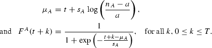
We now describe a hypothesized sampling scheme for the case where observations are limited to the number of currently infected individuals on a farm. Following the onset of an epidemic episode on a farm, we sample the number of infected animals on the farm at every discretized time step, starting at $\tau$, which, for convenience, we assume known. We assume that, for a particular farm, for a particular strain, the testing procedure allows us to infer the number of infecteds on the farm at that point in time, and employ the following scheme in order to extract F(t). For some t in $\tau , \tau +1, \ldots ,\tau +\gamma -1$, consider the sequence of observations (counts of infected) at lag $\gamma$, starting from t until the end of the episode. Let this be $l_t, l_{ t+\gamma }, \ldots l_{ t+(k-1)\gamma }$, where $k=\lfloor \frac{\omega -t}{\gamma } \rfloor$. Using (2), we get the system:

$$\begin{aligned} {\left\{ \begin{array}{ll} n_i F(t) &{}= l_t \\ n_i F(t+\gamma ) - n_i F(t) &{}= l_ {t+\gamma } \\ ...\\ n_i F(t+(k-1)\gamma ) - n_i F(t+(k-2)\gamma ) &{}= l_{ t+(k-1)\gamma } \\ \end{array}\right. } \end{aligned}$$

which solves to give

$$\begin{aligned} {\left\{ \begin{array}{ll} F(t) &{}= p_t \\ F(t+\gamma ) &{}= p_{t+\gamma } \\ ...\\ F(t+(k-1)\gamma ) &{}= p_{ t+(k-1)\gamma } \\ \end{array}\right. } \end{aligned}$$

(6)

where $p_j=\frac{l_{\tau }+l_{\tau +1}+\cdots +l_j}{n_i }$, $0 \le j < k$. Thus, we have estimates of $F(\cdot )$ for $\tau , \tau +1, \ldots ,\tau +\gamma -1$, and estimation can now proceed as described in Sect. 2.7.

1.2 IC model simulation algorithm

The following algorithm simulates an epidemic from the infectivity curve (farm level) model. For each farm, apart from its location on the lattice grid, we keep track of the number of animals susceptible to A and B left (call these $n_A, n_B$). We update these numbers between epidemic episodes, not within, so that they represent the carrying capacity for the current, or next, epidemic.

Step 1 :

Infect two randomly chosen individuals in the population, one with strain A, one with strain B ($t=0$). Initialize $n_A, n_B$ to 25 for each farm.

Step 2 :

For $t = 1$ to T: (T is the time both pathogens completely disappear)

–:

For each new infection event at time $t-1$, update the infectivity curve for that farm. Let a, b be the infection sizes for stains A and B from time $t-1$. Then, for a single strain infection (say A) compute

Similar equations are used for strain B. Now compute the curves $Y_t$ and $S_t$ for each of A and B using the formulas in Sect. 2.4.

–:

If the second strain entered a farm at $t-1$, use the formulas above for the infectivity curves with the expressions for $n_A$ and $n_B$ given in (7).

–:

For each susceptible farm where the pathogen is not present, compute the relevant probabilities of infection $P^*$ (e.g. $P^A, P^B or P^{A \vee B}$). Generate the number of new infections as Binomial$(S_t, P^*)$. For joint susceptibility, if the result is k unspecified infections ($k \ge 1$) decide how many are with strain A by generating another Binomial$(k, \frac{\varLambda ^A}{\varLambda ^A +\varLambda ^B} )$.

–:

Update a and b with the new infections, if any.

–:

If an epidemic episode is over ($Y_t \approx 0$), update $n_A, n_B$ for that farm.

Step 3 :

Return the complete infectivity and susceptibility curves $Y_t^i$ and $S_t^i$ for each of the two strains, for every farm i.

1.3 Justification for the expressions of $n_A, n_B$ in the case of a joint epidemic

Start from the logistic differential equation for growth of a single pathogen in a population, $\text{ d }I_t/\text{ d }t =1/s I_t (n-I_t),$ where n is the total size of the farm. In an infection with two strains the pathogens share the farm and curb each other’s growth. This is expressed as

$$\begin{aligned} {\left\{ \begin{array}{ll} \text{ d }I_t^A/\text{ d }t &{}=1/s_A I_t^A (n-I_t^A-I_t^B), \text{ and } \\ \\ \text{ d }I_t^B/\text{ d }t &{}=1/s_B I_t^B (n-I_t^A-I_t^B). \end{array}\right. } \end{aligned}$$

In these equations, we see that the relative growth, $\frac{dI_t}{dt}/I_t$, for each strain, is the same upto a constant factor. From this, we obtain

$$\begin{aligned} \frac{n_A}{a}= \left( \frac{n_B}{b} \right) ^\frac{s_B}{s_A}. \end{aligned}$$

Adding the constraint that both strains share the entire farm, namely $n_A+n_B=n$, we get a system of two equations in two unknowns. An approximate solution is

$$\begin{aligned} {\left\{ \begin{array}{ll} n_A = \dfrac{ns_Ba+ab(s_A-s_B)}{s_Ab+s_Ba} \\ \\ n_B = \dfrac{ns_Ab+ab(s_B-s_A)}{s_Ab+s_Ba}. \end{array}\right. } \end{aligned}$$

(7)

For simplicity, we also make the assumption that given the final sizes $n_A$ and $n_B$, the growth curve for each individual strain is logistic, and hence we can use these values directly in the simulation algorithm and proceed as if the strains were independent.

1.4 Data analyses for alternative parameter settings

We summarize the fit of the farm level model to data generated from the animal level model under another set of parameters here; this is an example of a less infectious disease system. The parameter values used in the animal level model to simulate these data are: $\alpha _A=0.001, \alpha _B=0.0005, \beta =2, \delta _A=0.1$, and $\delta _B=0.05$ (which correspond to approximate $R_0$ values of 2.5 for strain A, and 1.3 for strain B). In addition, the cross-immunity period is set to $\phi _{AB}=\phi _{BA}=10$. Parameter estimation for the farm level model using one simulated dataset is given in Table 3, and a sample epidemic curve is shown in Fig. 7. Posterior predictive plots (similar to the ones in the results section) are given in Figs. 8, 9 and 10.

Fig. 7

Sample epidemic curve for one farm infected with strain A. Points represent the actual number of infected animals on the farm

Fig. 8

Joint epidemic size distributions (strains A and B), for parameters $\alpha _A=0.001, \alpha _B=0.0005, \beta =2, \delta _A=0.1, \delta _B=0.05$: center panel-true distribution; outer panels-posterior predictive based on eight replicated datasets (these are marked by a diamond)

Fig. 9

Empirical density of epidemic ‘spread’ at time $t=5$, for strain A (left plot) and B (right plot). True density is represented by a continuous line, posterior predictive densities by dashed lines

Fig. 10

Empirical c.d.f. of the time of last infection: strain A (left plot) and B (right plot). True distribution is represented by a continuous line, posterior predictive distributions by dashed lines

Table 3 Parameter estimates for the farm level model for a lower pathogenicity dataset

References

Abu-Raddad LJ, Ferguson NM (2004) The impact of cross-immunity, mutation and stochastic extinction on pathogen diversity. Proc R Soc Lond B 271(1556):2431–2438
Ackerman E, Longini IM, Seaholm SK, Hedin AS (1990) Simulation of mechanisms of viral interference in influenza. Int J Epidemiol 19:444–454
Andreasen V, Lin J, Levin SA (1997) The dynamics of cocirculating strains conferring partial cross-immunity. J Math Biol 35:825–842
Bartlett MS (1956) Deterministic and stochastic models for recurrent epidemics. In: Neyman J (ed) Proceedings of the Third Berkeley Symposium on Mathematical Statistics and Probability, vol 4. University of California Press, pp 81–109
Cauchemez S, Bhattarai A, Marchbanks TL, Fagan RP, Ostroff S, Ferguson NM et al (2011) Role of social networks in shaping disease transmission during a community outbreak of 2009 H1N1 pandemic influenza. Proc Natl Acad Sci 108(7):2825–2830
Chis Ster I, Dodd PJ, Ferguson NM (2012) Within-farm transmission dynamics of foot and mouth disease as revealed by the 2001 epidemic in Great Britain. Epidemics 4(3):158–169
Chis Ster I, Singh BK, Ferguson NM (2009) Epidemiological inference for partially observed epidemics: the example of the 2001 foot and mouth epidemic in Great Britain. Epidemics 1(1):21–34
Clancy CF, O’Callaghan MJA, Kelly TC (2006) A multi-scale problem arising in a model of avian flu virus in a seabird colony. J Phys Conf Ser, 55(1):45. IOP Publishing
Cisternas J, Gear CW, Levin SA, Kevrekidis IG (2004) Equation-free modelling of evolving diseases: coarse-grained computations with individual-based models. Proc R Soc Lond A 460:2761–2779
Deardon R, Brooks SP, Grenfell BT, Keeling MJ, Tildesley MJ, Savill NJ, Shaw DJ, Woolhouse MEJ (2010) Inference for individual-level models of infectious diseases in large populations. Stat Sin 20(1):239–261
Dietz K (1979) Epidemiologic interference of virus populations. J Math Biol 8(3):291–300
Ferguson NM, Donnelly CA, Anderson RM (2001) The foot-and-mouth epidemic in Great Britain: pattern of spread and impact of interventions. Science 292(5519):1155–1160
Ferguson NM, Galvani AP, Bush RM (2003) Ecological and immunological determinants of influenza evolution. Nature 422:428–433
Gelman A, Meng XL, Stern HS (1996) Posterior predictive assessment of model fitness via realized discrepancies (with discussion). Stat Sin 6:733–807
Gog JR, Swinton J (2002) A status-based approach to multiple strain dynamics. J Math Biol 44:169–184
Grenfell B, Harwood J (1997) (Meta) population dynamics of infectious diseases. Trends Ecol Evol 12(10):395–399
Groendyke C, Welch D, Hunter DR (2012) A network-based analysis of the 1861 Hagelloch measles data. Biometrics 68(3):755–765
Jandarov R, Haran M, Bjrnstad O, Grenfell B (2014) Emulating a gravity model to infer the spatiotemporal dynamics of an infectious disease. J R Stat Soc Ser C (Applied Statistics) 63(3):423–444
Jegat C, Carrat F, Lajaunie C, Wackernagel H (2008) Early detection and assessment of epidemics by particle filtering. In: geoENV VIGeostatistics for environmental applications. Springer, Netherlands, pp 23–35
Jewell CP, Kypraios T, Neal P, Roberts GO (2009) Bayesian analysis for emerging infectious diseases. Bayesian Anal 4:191–222
Kryazhimskiy S, Dieckmann U, Levin SA, Dushoff J (2007) On state-space reduction in multi-strain pathogen models, with an application to antigenic drift in influenza A. PLoS Comput Biol 3(8):e159. doi:10.1371/journal.pcbi.0030159
Madden LV (1980) Quantification of disease progression. Prot Ecol 2:159–176
Paul M, Held L, Toschke AM (2008) Multivariate modelling of infectious disease surveillance data. Stat Med 27(29):6250–6267
Potter MA, Brown ST, Lee BY, Grefenstette J, Keane CR, Lin CJ et al (2012) Preparedness for pandemics: does variation among states affect the nation as a whole? J Public Health Manag Pract 18(3):233
Stegeman A, Bouma A, Elbers AR, de Jong MC, Nodelijk G, de Klerk F, Koch G, van Boven M (2004) Avian influenza A virus (H7N7) epidemic in The Netherlands in 2003: course of the epidemic and effectiveness of control measures. J Infect Dis 190(12):2088–2095
Yang Y, Halloran ME, Daniels MJ, Longini IM, Burke DS et al (2010) Modeling competing infectious pathogens from a bayesian perspective: Application to inuenza studies with incomplete laboratory results. J Am Stat Assoc 105(492):1310–1322. doi:10.1198/jasa.2010.ap09581
Acknowledgments
This work was funded by OMAFRA/UoG Partnership, OMAFRA HQP Scholarship Program, NSERC, and equipment was provided by the CFI grant, “Centre for Public Health and Zoonoses”.
Author information
Authors and Affiliations
Corresponding author