Index appearance record with preorders

Abstract

Transforming $\omega$-automata into parity automata is traditionally done using appearance records. We present an efficient variant of this idea, tailored to Rabin automata, and several optimizations applicable to all appearance records. We compare the methods experimentally and show that our method produces significantly smaller automata than previous approaches.

1 Introduction

Constructing correct-by-design systems from specifications given in linear temporal logic (LTL) [34] is a classical problem [35], called LTL (reactive) synthesis. The automata-theoretic solution to this problem is to translate the LTL formula to a deterministic automaton and solve the corresponding game on the automaton. Although different kinds of automata can be used, a reasonable choice would be deterministic parity automata (DPA) due to the practical efficiency of parity game solvers [12, 28] and the fact that these games allow for optimal memoryless strategies. The bottleneck is thus to create a reasonably small DPA. The classical way to transform LTL formulae into DPA is to first create a non-deterministic Büchi automaton (NBA) and then determinize it [15]. Since determinization procedures [32, 40] based on Safra’s construction [38] are practically inefficient, many alternative approaches to LTL synthesis arose, trying to avoid determinization and/or focusing on fragments of LTL, e.g. [1, 22, 33]. However, new results on translating LTL directly and efficiently into deterministic automata [9, 10, 17] open new possibilities for the automata-theoretic approach. Indeed, tools such as Rabinizer [16, 20] or LTL3DRA [2] can produce practically small deterministic Rabin automata (DRA). Consequently, the task is to efficiently transform DRA into DPA, which is the aim of this paper.

Transformations of deterministic automata into DPA are mostly based on appearance records [13]. For instance, for deterministic Muller automata (DMA), one wants to track which states appear infinitely often and which do not. In order to do that, the state appearance record keeps a permutation of the states, ordered according to their most recent visits, see e.g. [23, 41]. In contrast, for deterministic Streett automata (DSA), one only wants to track which sets of states are visited infinitely often and which not. Consequently, index appearance record (IAR) keeps a permutation of these sets of interest instead, which are typically very few. Such a transformation has been given first in [39] from DSA to DRA only (not DPA, which is a subclass of DRA). Fortunately, this construction can be further modified into a transformation of DSA to DPA, as shown in [23].

Since (i) DRA and DSA are syntactically the same, recognizing the complement languages of each other, and (ii) DPA can be complemented without any cost, one can apply the IAR of [23] to DRA, too. However, the construction presented in [23] is suboptimal in several regards. In this work, we present a view on appearance records that is more natural for DRA, resulting in a much more efficient transformation.

Our contribution in this paper is as follows:

• We provide an efficient IAR construction transforming DRA to DPA, generalizing previous works. In particular, we show that the construction of [21] shares the underlying idea of [23], while the IAR presented now generalizes both.

• We present several optimizations applicable to appearance-record constructions in general. A canonic representation of “simultaneous” events significantly reduces the state space size and allows for further optimizations.

• We experimentally compare our IAR construction to the construction of [23] and evaluate the effect of the different optimizations. Moreover, we combine IAR with the LTL$\rightarrow$DRA tool of Rabinizer [20] and Spot [7] to obtain LTL$\rightarrow$DRA$\rightarrow$DPA translation chains and compare it to state-of-the-art tools for LTL$\rightarrow$DPA translation offered by Rabinizer/Owl¹ and Spot, confirming its competitiveness.

2 Preliminaries

As usual, $\mathbb {N}$ refers to the (positive) natural numbers. For every set S, we use $\overline{S}$ to denote its complement. Moreover, $S^\star$ and $S^\omega$ refer to the set of finite and infinite sequences comprising elements of S, respectively.

2.1 $\omega$-Automata

An alphabet is a finite set $\varSigma$. The elements of $\varSigma$ are called letters. An (in)finite word is an (in)finite sequence of letters. The set of all finite and infinite words over $\varSigma$ is given by $\varSigma ^*$ and $\varSigma ^\omega$, respectively. A set of words $\mathcal {L}\subseteq \varSigma ^\omega$ is called (infinite) language. The length of a word w, denoted $\vert w\vert$, is given by the number of its letters, setting $\vert w\vert = \infty$ for infinite words $w \in \varSigma ^\omega$. The ith letter ($i \le \vert w\vert$) of a word w is denoted by $w_i$, i.e. $w = w_1 w_2 \cdots$.

Definition 2.1

(Deterministic $\omega$-Automata) A deterministic $\omega$-automaton $\mathcal {A}$ over the alphabet $\varSigma$ is given by a tuple $(Q, \varSigma , \delta , q_0, \alpha )$ where

• $Q$ is a finite set of states,

• $\varSigma$ is an alphabet,

• $\delta : Q\times \varSigma \rightarrow Q{\cup }\{\bot \}$ is a transition function where $\bot$ represents that no transition is defined for the given state and letter,

• $q_0\in Q$ is the initial state, and

• $\alpha$ is an acceptance condition (described later).

The transition function $\delta$ induces the set of transitions $\varDelta = \{\langle q, a, q'\rangle \mid q \in Q, a \in \varSigma , q' = \delta (q, a) \in Q\}$. We write $\mathcal {A}_q = (Q, \varSigma , \delta , q, \alpha )$ to denote the automaton with new initial state q.

We identify automata with the underlying graph induced by the transition structure. For a transition $t = \langle {q},{a},{q'}\rangle \in \varDelta$ we say that t starts at q, moves under a and ends in $q'$. A sequence of transitions $\rho = \rho _1 \rho _2 \cdots \in \varDelta ^\omega$ is an (infinite) run of an automaton $\mathcal {A}$ on a word $w \in \varSigma ^\omega$ if (i) $\rho _1$ starts at $q_0$, and (ii) for each i we have that $\rho _i$ moves under $w_i$ and ends in the same state as $\rho _{i+1}$ starts at. We write $\mathcal {A}(w)$ to denote the unique run of $\mathcal {A}$ on w, if it exists. Such a run may not exist if at any point the transition function $\delta$ yields $\bot$. If an automaton $\mathcal {A}$ has a run for every word $w \in \varSigma ^\omega$, it is called complete.

A transition t occurs in $\rho$ if there is some i with $\rho _i = t$. By ${{\,\mathrm{Inf}\,}}(\rho )$ we denote the set of all transitions occurring infinitely often in $\rho$. Additionally, we extend ${{\,\mathrm{Inf}\,}}$ to words by defining ${{\,\mathrm{Inf}\,}}_{\mathcal {A}}(w) = {{\,\mathrm{Inf}\,}}(\mathcal {A}(w))$ if $\mathcal {A}$ has a run on w. If $\mathcal {A}$ is clear from the context, we furthermore write ${{\,\mathrm{Inf}\,}}(w)$ for ${{\,\mathrm{Inf}\,}}_{\mathcal {A}}(w)$.

An acceptance condition is a positive Boolean formula, i.e. only comprising variables, logical and, and logical or, over the variables $V_\varDelta = \{{{\,\mathrm{Inf}\,}}[T], {{\,\mathrm{Fin}\,}}[T] \mid T \subseteq \varDelta \}$. Acceptance conditions are interpreted as follows. Given a run $\rho$ and an acceptance condition $\alpha$, we consider the truth assignment that sets the variable ${{\,\mathrm{Inf}\,}}[T]$ to true iff $\rho$ visits (some transition of) T infinitely often, i.e. ${{\,\mathrm{Inf}\,}}(\rho ) {\cap }T \ne \emptyset$. Dually, ${{\,\mathrm{Fin}\,}}[T]$ is set to true iff $\rho$ visits every transition in T finitely often, i.e. ${{\,\mathrm{Inf}\,}}(\rho ) {\cap }T = \emptyset$. A run $\rho$ satisfies $\alpha$ if this truth-assignment evaluates $\alpha$ to true. We say that an automaton accepts a word $w \in \varSigma ^\omega$ if its run $\rho$ on w satisfies the automaton’s acceptance condition $\alpha$. The language of $\mathcal {A}$, denoted by $\mathcal {L}(\mathcal {A})$, is the set of words accepted by $\mathcal {A}$. An automaton recognizes a language $\mathcal {L}$ if $\mathcal {L}(\mathcal {A}) = \mathcal {L}$. Many kinds of acceptance conditions have been defined in the literature, e.g. Muller [30], Rabin [36], Streett [44], Parity [29], and generalized Rabin [17]. In this work, we primarily deal with Rabin and Parity. A Rabin condition $\{(F_i, I_i)\}_{i=1}^k$ yields an acceptance condition $\alpha = \bigvee _{i=1}^k ({{\,\mathrm{Fin}\,}}[F_i] \wedge {{\,\mathrm{Inf}\,}}[I_i])$. Each $(F_i, I_i)$ is called a Rabin pair, where the $F_i$ is called the prohibited set (or Finite set) and $I_i$ the required set (Infinite set), respectively.² A Parity or Rabin chain condition is a Rabin condition where $F_1 \subseteq I_1 \subseteq \cdots \subseteq F_k \subseteq I_k$. This condition is equivalently specified by a priority assignment $\lambda : \varDelta \rightarrow \mathbb {N}$. A word is accepted iff on its run $\rho$ the maximum priority of all infinitely often visited transitions $\max \{\lambda (q) \mid q \in {{\,\mathrm{Inf}\,}}(\rho )\}$ is even.³

By slight abuse of notation, we identify the acceptance condition with the above set/priority representations. A deterministic Rabin or parity automaton is a deterministic $\omega$-automaton with an acceptance condition of the corresponding kind. In the rest of the paper we use the corresponding abbreviations DRA and DPA.

Furthermore, given a DRA with an acceptance set $\{(F_i, I_i)\}_{i=1}^k$ and a word $w \in \varSigma ^\omega$, we write $\mathcal {F}_{\inf }(w) = \{F_i \mid F_i {\cap }{{\,\mathrm{Inf}\,}}(w) \ne \emptyset \}$ and $\mathcal {I}_{\inf }(w) = \{I_i \mid I_i {\cap }{{\,\mathrm{Inf}\,}}(w) \ne \emptyset \}$ to denote the set of all infinitely often visited prohibited and required sets, respectively.

Remark 2.1

In this work, we restrict ourselves to deterministic automata. A non-deterministic automaton can have multiple transitions for a given state-letter pair, and a word is accepted if any of its possible runs is accepting. However, non-deterministic variants of both Rabin and parity automata are rarely used in practice, while deterministic parity automata are a fundamental tool to, for example, LTL synthesis, as explained in the introduction. Thus, we focus on deterministic automata for the sake of simplicity and practicality. Nevertheless, our methods and proofs can be directly extended to non-deterministic automata.

2.1.1 State-based acceptance

Traditionally, acceptance for $\omega$-automata is defined state-based, i.e. the acceptance condition is formulated in terms of states instead of transitions. For example, a state-based parity acceptance would assign a priority to each state and a word is accepted if the maximal priority among the infinitely often visited states is even. One of the main reasons for this state-based view is that the acceptance of finite automata is defined via states in which the run of the (finite) word ends. Since the concept of $\omega$-automata is rooted in finite automata, this approach is carried over to the infinite domain. However, in line with recent works, e.g. [6, 7, 20], we instead use transition-based acceptance for two reasons.

Firstly, transition-based acceptance is both theoretically and practically more concise. It is straightforward to convert from state-based acceptance to transition-based acceptance by “pushing” the acceptance information onto the outgoing transitions. This does not incur an increase in the number of states, i.e. transition-based automata are always at least as concise as state-based automata. For the other direction observe that when defining the acceptance on transitions, we can “access” both the current and the next state, while state-based acceptance only allows reasoning about the current state. The natural translation from transition-based to state-based thus needs to “remember” the previous state and transition, i.e. essentially uses $Q\times \varSigma$ as new-state space. In practice, the alphabet is often derived from a set of atomic propositions $\mathsf {AP}$, i.e. $\varSigma = 2^{\mathsf {AP}}$. Thus, going from $Q$ to $Q\times 2^{\mathsf {AP}}$ results in an exponential blow-up in the number of states. We also provide a matching lower bound: Theorem 2.1 outlines a family of single-state transition-based automata where every state-based automaton recognizing the same language necessarily has an exponential number of states.

Secondly, many constructions are more “natural” to formulate using transition-based acceptance. Informally, acceptance information is often based on the change of state instead of the actual “label” of a particular state. In particular, the (state-based) construction of [23], which inspired our work, adds information to the state space based on the previous state. However, this information is only used to deduce acceptance information. By carefully transforming this construction to transition-based acceptance, we actually arrive at the same construction as the one presented in the conference paper [21], despite approaching the problem from different directions. We explain this transformation in more detail later on, see Sect. 3.2. Observing this underlying equivalence when considering state-based acceptance is far less obvious, since the type of “meta-data” stored by these constructions is significantly different. As such, thinking in terms of transition-based acceptance can aid understanding the construction by emphasizing the difference between state and transition information. However, we repeat that this is not a hard fact but rather an informal observation.

Theorem 2.1

There exists a family of languages $\mathcal {L}_n$ which are recognized by an automaton with transition-based Rabin acceptance using a single state, while every automaton with state-based Rabin acceptance requires at least $2^n$ states.

Proof

(Sketch) Fix the alphabet $\varSigma _n = \{1, \dots , 2^n\}$. Moreover, define the language $\mathcal {L}_n \subseteq \varSigma _n^\omega$ to contain exactly all finally constant words $w \in \varSigma _n^\omega$, i.e. $\mathcal {L}_n = \{w \mid \exists k.~\forall k' > k.~w_k = w_{k'}\}$.

This language can be recognized by a (transition-based) DRA with a single state $q_0$ and a self-loop under every letter. A word w is finally constant iff there exists a letter $v \in \varSigma _n$ such that $w_k = v$ for all sufficiently large k. So, intuitively, we can create a Rabin pair for every way a word can be stable. Formally, for every letter $v \in \varSigma _n$, we define $F_v = \{(q_0, v', q_0) \mid v' \ne v\}$ and $I_v = \{(q_0, v, q_0)\}$. When restricted to state-based acceptance, it is not difficult (but tedious) to see that $2^n$ states are necessary (and sufficient). Intuitively, the state-based acceptance needs to “remember” the previous letter in order to detect every switching behaviour. If there were less than $2^n$ states, we can construct two accepted words which visit the same set of states infinitely often. By appropriately switching back and forth between these two words, we obtain another accepted word, which contradicts the non-alternation requirement of the language. $\square$

There are some subtleties to be noted. One may claim that transition-based acceptance is “cheating”: We are not making the automaton smaller as a whole, we are only moving complexity into the transitions and acceptance; clearly an exponential factor cannot magically vanish. In particular, the language from Theorem 2.1 can be recognized by an automaton with $2^n + 1$ states and a single Rabin pair, compared to the $2^n$ pairs of the transition-based automaton. However, there are a number of practical arguments why a compact state space often is preferable over a simpler transition relation. The details are beyond the scope of this work, and we only give a brief overview on major points. From a theoretical side, the complexity of algorithms may depend differently on the number of states and, for example, size of the acceptance condition. Indeed, reducing the number of states often yields more speed-ups in practice than a corresponding simplification of the transition relation. In particular, applications of automata often end up building the product between a labelled system and an automaton. There, we usually are only interested in the acceptance information associated with states in the product. Thus, we can project away large parts of the transition relation after building the product, while the states of the automaton remain a part of the product. Also, representing the transition relation together with acceptance information symbolically works well in practice (see, for example, [19]) and is much easier to achieve than a similar generic approach applied to the set of states. We emphasize that (apart for parametrized algorithms) these are purely empirical/anecdotal arguments, a different representation naturally does not change the computational complexity of associated decision problems.

2.1.2 Strongly connected components

A non-empty set of states $S \subseteq Q$ in an automaton $\mathcal {A}$ is strongly connected if for every pair $q, q' \in S$ there is a path (of non-zero length) from q to $q'$. Such a set S is a strongly connected component (SCC) if it is maximal w.r.t. set inclusion, i.e. there exists no strongly connected $S'$ with $S \subsetneq S'$. Consequently, SCCs are disjoint.

SCCs are an important concept for analysing the language of an automaton. Recall that acceptance of a word by an $\omega$-automaton only depends on the set of transitions visited infinitely often by its run. This set of infinitely often visited transitions necessarily has to contain a cycle and thus the corresponding set of states is strongly connected. In particular, ${{\,\mathrm{Inf}\,}}(w)$ always belongs to a single SCC. In other words, only states and transitions in SCCs are relevant for acceptance, since only those can be encountered infinitely often. We say that a state is transient if it does not belong to any SCC. Similarly, a transition is called transient if its starting or end state does not belong to an SCC or these states belong to two different SCCs. Transient objects are encountered at most once along every path.

2.2 Preorders

In this work, we make heavy use of (total) preorders over finite sets. Thus, we introduce some notation.

Definition 2.2

Let S be a finite set. A binary relation $\precsim \subseteq S \times S$ is called preorder (or quasiorder) if it is reflexive, i.e. $a \precsim a$ for all $a \in S$, and transitive, i.e. $a \precsim b$ and $b \precsim c$ implies $a \precsim c$ for all $a, b, c \in S$. It is called total if for all $a, b \in S$ we additionally have $a \precsim b$ or $b \precsim a$. We write $a \mathbin {\sim }b$ if $a \precsim b$ and $b \precsim a$, i.e. a and b are “equal” under $\precsim$. Dually, we write $a \prec b$ if $a \precsim b$ but not $b \precsim a$, i.e. a is “smaller” than b under $\precsim$.

We use $\varXi ^k$ to denote the set of all total preorders on $S = \{1, \dots , k\}$.

We exclusively use total preorders; hence, we omit “total” for the sake of readability. These (total) preorders are also called / are equivalent to weak orderings or (weak) preference relations. Such orders can, for example, be interpreted as an age relation, where $a \mathbin {\sim }b$ means a and b are “of the same age” and $a \prec b$ means a is “younger” than b or “occurred more recently”. We use this intuition while explaining our algorithms.

Note that a preorder partitions the set S into equivalence classes (elements of equal age) and assigns a total order to these classes. More specifically, for every preorder, there exists a unique ordered partitioning $(E_p)_{p=1}^r \subseteq S$ (where r depends on $\precsim$) such that

• $E_p \ne \emptyset$ for all $1 \le p \le r$,

• $a \mathbin {\sim }b$ iff $a, b \in E_p$ for some $1 \le p \le r$,

• $a \prec b$ iff $a \in E_p$, $b \in E_q$ for some $1 \le p < q \le r$

and vice versa. We call r the size of $\precsim$, denoted by $\vert \precsim \vert$ and write $\precsim [p]$ to refer to the pth class $E_p$ for $1 \le p \le \vert \precsim \vert$. Naturally, the number of (total) preorders is given by $\vert \varXi ^k\vert = \sum _{i=0}^k i! \cdot S(k, i)$, where S(k, i) are the Stirling numbers of the second kind, i.e. the number of ways to partition a set of k objects into i non-empty subsets. The value $\vert \varXi ^k\vert$ is also called ordered Bell number or Fubini number.

As an example, consider the preorder specified by $\precsim = (\{1\}, \{2, 3\}, \{4\}) \in \varXi ^4$. Here, we have $1 \prec 2 \mathbin {\sim }3 \prec 4$. For a preorder $\precsim \in \varXi ^k$, we write $\mathrm {pos}(\precsim , i)$ to denote the position of i in $\precsim$, i.e. the index p with $i \in \precsim [p]$. Moreover, we write $\mathrm {off}(\precsim , i) := \vert \{j \mid j \precsim i\}\vert = \vert \{j \mid \mathrm {pos}(\precsim , j) \le \mathrm {pos}(\precsim , i)\}\vert$ to denote the offset of i, i.e. the number of elements less or equal to i. Considering the above preorder $\precsim$ again, we for example have that $\mathrm {pos}((\{1\}, \{2, 3\}, \{4\}), 2) = 2$, since 2 is in the second equivalence class, and $\mathrm {off}((\{1\}, \{2, 3\}, \{4\}), 2) = 3$, since there are three elements less than or equal to 2, namely 1, 2, and 3. We also make use of a reordering operation described in the following. Let $\precsim \in \varXi ^k$ be a preorder and $G \subseteq \{1, \dots , k\}$. We define $\precsim ' = \mathrm {move}(\precsim , G)$ as the preorder obtained by “moving” all elements of G to the front. Intuitively, $\precsim '$ is the preorder where all elements of G are “reborn” and thus younger than all others. Formally, we set $\precsim ' = (G, \precsim [1] \setminus G, \precsim [2] \setminus G, \dots , \precsim [\vert \precsim \vert ] \setminus G)$, omitting empty sets. With the above example $\precsim = (\{1\}, \{2, 3\}, \{4\})$, we get that $\mathrm {move}(\precsim , \{1, 2\}) = (\{1, 2\}, \{3\}, \{4\})$. Note that the preorder obtained this way can have a length anywhere between 1 and $\vert \precsim \vert + 1$.

Finally, we define the notion of refinement. Given two preorders $\precsim , \precsim ' \in \varXi ^k$, we say that $\precsim$ refines $\precsim '$ if $\precsim \subseteq \precsim '$ and $\precsim$ strictly refines $\precsim '$ if $\precsim \subsetneq \precsim '$. Intuitively, this means that $\precsim$ is more “restrictive”. Another way to view refinement is that some previously equal items are now considered different. For example, we have that $(\{1, 2\}, \{3, 4\})$ is refined by $(\{1\}, \{2\}, \{3, 4\})$ but not by $(\{1\}, \{2, 3\}, \{4\})$, since the latter preorder considers 2 and 3 to be equal.

3 Index appearance record

In order to translate (state-based acceptance) Muller automata to parity automata, a construction called latest appearance record (or state appearance record) [4, 13] has been devised.⁴ In essence, the constructed state space consists of permutations of all states in the original automaton. In each transition, the state which has just been visited is moved to the front of the permutation. From this, one can deduce the set of all infinitely often visited states by investigating which states change their position in the permutation infinitely often along the run of the word. This constraint can be encoded as parity condition.

However, this approach comes with a very fast growing state space, as the amount of permutations grows exponentially in the number of input states. Moreover, applying this idea to transition-based acceptance leads to even faster growth, as there usually are a lot more transitions than states. In contrast to Muller automata, the exact set of infinitely often visited transitions is not needed to decide acceptance of a word by a Rabin automaton. It is sufficient to know which of the prohibited and required sets are visited infinitely often.⁵ Hence, index appearance record uses the indices of the Rabin pairs instead of particular states in the permutation construction. This provides enough information to decide acceptance.

Definition 3.1

Let $\mathcal {R}= (Q, \varSigma , \delta , q_0, \{(F_i, I_i)\}_{i=1}^k)$ be a Rabin automaton. Then the index appearance record automaton $\mathsf {IAR}(\mathcal {R}) = (\tilde{Q}, \varSigma , \tilde{\delta }, \tilde{q}_0, \lambda )$ is defined as a parity automaton with

• $\tilde{Q}= Q\times \varXi ^k$,

• $\tilde{q}_0= (q_0, (\{1, \dots , k\}))$, and

• $\tilde{\delta }((q, \precsim ), a) = (\delta (q, a), \mathrm {move}(\precsim , \{i \mid t \in F_i\}))$ where $t = \langle q,a,\delta (q, a)\rangle$ is the corresponding transition in the Rabin automaton, i.e. all indices of prohibited sets visited by the transition t are moved to the front. We set $\tilde{\delta }((q, \precsim ), a) = \bot$ if $\delta (q, a) = \bot$.

• To define the priority assignment, we first introduce some auxiliary notation. Fix a transition $\tilde{t} = \langle (q,\precsim ),{a},{(q', \precsim ')}\rangle$ and its corresponding transition $t = \langle {q},{a},{q'}\rangle$ in the Rabin automaton. Let $e = \max _{\precsim } \{i \mid t \in F_i {\cup }I_i\}$ the largest index w.r.t. $\precsim$ of a Rabin pair containing t or $e = 0$ if no such pair exists. We define ${{\,\mathrm{maxPos}\,}}(\tilde{t}) = \mathrm {pos}(\precsim , e)$ (or 0 if $e = 0$) and analogously ${{\,\mathrm{maxOff}\,}}(\tilde{t}) = \mathrm {off}(\precsim , e)$ (or 0 if $e = 0$) the position and offset of e in $\precsim$. For readability, set $o = {{\,\mathrm{maxOff}\,}}(\tilde{t})$ and $p = {{\,\mathrm{maxPos}\,}}(\tilde{t})$. Then, we define the priority assignment by

  $$\begin{aligned} \lambda (\tilde{t}) := {\left\{ \begin{array}{ll} 1 &{} \hbox {if }\;e = 0, \\ 2 o &{} \hbox {if}\; \forall i \in \precsim [p].~t \notin F_i, \\ 2 o + 1 &{} \hbox {otherwise, i.e.\ if} \;\exists i \in \precsim [p].~t \in F_i. \end{array}\right. } \end{aligned}$$

  Note that the second case implies that there exists an $i \in \precsim [p]$ such that $t \in I_i$, as otherwise ${{\,\mathrm{maxPos}\,}}(\tilde{t})$ would have a different value.

For a practical implementation, one would of course only construct the states reachable from the initial state. We define the state space as the whole product for notational simplicity. When drawing examples and discussing practical issues like (space) complexity or the actual implementation, we only consider the set of reachable states.

Furthermore, for readability, we identify Rabin sets $F_i$ and $I_i$, with their index i. For example, given a preorder $\precsim$ we say that “$F_i$ is younger than $F_j$” if $i \prec j$ or say write “the position of $F_i$” to refer to $\mathrm {pos}(\precsim , i)$.

Remark 3.1

We highlight that our construction does not fundamentally modify the state space of the input automaton. Instead, it only augments the original states with additional metadata. In particular, if the states of the Rabin automaton are meaningful objects, our construction preserves this meaning. This is, for example, relevant for recent approaches exploiting semantic labelling [18] obtained from the Rabin automaton [9] or reduction approaches relying on knowledge about states [25].

Before proving correctness, i.e. that $\mathsf {IAR}(\mathcal {R})$ recognizes the same language as $\mathcal {R}$, we provide a small example in Fig. 1 and explain the intuition behind the construction. For a given run, the indices of all prohibited sets which are visited infinitely often will eventually be younger than all those only seen finitely often: After some finite number of steps, none of the finitely often visited ones will be seen again, while the infinitely occurring ones will be moved to the front over and over again. By choice of priorities, we only accept a word if additionally some required set older than all infinitely often seen prohibited sets also occurs infinitely often.

Fig. 1

An example DRA and the resulting IAR DPA. For readability, we only draw the reachable part of the state space. In the Rabin automaton, a number in a white box next to a transition indicates that this transition is a required one of that Rabin pair. A black shape dually indicates that the transition is an element of the corresponding prohibited set. For example, with $t = \langle p,a,p\rangle$, we have $t \in F_1$ and $t \in I_2$. In the IAR construction, we shorten the notation for preorders to save space. For example, “p 12” corresponds to $(p, (\{1, 2\}))$ and “p 1|2” to $(p, (\{1\}, \{2\}))$. The priority of a transition is written next to the transitions’ letter

In contrast to the constructions of [21, 23], we consider total preorders instead of permutations (corresponding to total orders). For state appearance records, which inspired these constructions, it is natural to use a permutation, since exactly one state appears in each step. However, with Rabin acceptance it might happen that two prohibited sets are visited at the same time. The previous constructions resorted to breaking this tie arbitrarily. This suggests that permutations are not the natural mechanism to track the order of appearance for such events. Therefore, we instead use preorders, which are able to represent such ties.

The curious reader may wonder how this construction improves the one of [21], especially since applying the construction of [21] to the example in Fig. 1 yields a smaller automaton. Indeed, in the current form, the automaton $\mathsf {IAR}(\mathcal {R})$ always is at least as large as the one produced by [21] (with initial state optimization included) and can even be significantly worse: Intuitively, every “unresolved” tie either gets resolved eventually or remains unresolved. In the former case, an additional useless state is introduced, and in the latter we may as well have resolved it arbitrarily immediately. However, by using an optimization based on refinement, we recover the worst-case complexity of [21] through the above intuition and obtain significant savings in practice.

3.1 Proof of correctness

We now prove correctness of our construction. Thus, for the rest of the section fix a Rabin automaton $\mathcal {R}= (Q, \varSigma , \delta , q_0, \{(F_i, I_i)\}_{i=1}^k)$ and let $\mathcal {P}= \mathsf {IAR}(\mathcal {R}) = (\tilde{Q}, \varSigma , \tilde{\delta }, \tilde{q}_0, \lambda )$ the constructed IAR automaton. First, we show that runs are preserved between the two automata.

Lemma 3.1

Let $q \in Q$ be a state in $\mathcal {R}$ and $(q, \precsim ) \in \tilde{Q}$ an IAR state with q as first component. Then, $\delta (q, a) = q'$ iff $\tilde{\delta }((q, \precsim ), a) = (q', \precsim ')$ for some $\precsim ' \in \varXi ^k$ (and $\delta (q, a) = \bot$ iff $\tilde{\delta }((q, \precsim ), a) = \bot$).

Proof

Follows immediately from the definition. $\square$

Corollary 3.1

A word $w \in \varSigma ^\omega$ has a run $\rho$ on $\mathcal {R}$ iff it has a run $\tilde{\rho }$ on $\mathcal {P}$. Moreover, if such a pair of runs exists, we have that $\rho _i = q$ iff $\tilde{\rho }_i = (q, \precsim )$ for some $\precsim \in \varXi ^k$.

Proof

Follows from Lemma 3.1 using an inductive argument. $\square$

Note that the above statement essentially shows that the first component of the IAR state stays “in sync” with the Rabin automaton. Now, we show how the preorders evolve in the infinite run. In particular, all infinitely often seen prohibited sets eventually are younger than all finitely often seen ones.

Lemma 3.2

Let $w \in \varSigma ^\omega$ be a word on which $\mathcal {P}$ has a run $\tilde{\rho }$. Then, the offsets of all finitely often visited prohibited sets stabilize after a finite number of steps, i.e. their offset is identical in all infinitely often visited states. Moreover, for every i, j with $F_i \in \mathcal {F}_{\inf }(w)$, $F_j \notin \mathcal {F}_{\inf }(w)$ and infinitely often seen state $(q, \precsim )$, we have that $i \prec j$, i.e. all infinitely often seen prohibited sets are younger than all finitely often ones in every infinitely often visited state.

Proof

The offset of an index i only changes in two different ways:

• $F_i$ has been visited and thus i is moved to the front, or

• some $F_j$ with a position greater to the one of $F_i$, i.e. $i \prec j$, has been visited and is moved to the front, increasing the offset of $F_i$.

Note that visiting a set $F_j$ with $i \mathbin {\sim }j$ does not increase the offset of i.

Let $\rho$ be the run of $\mathcal {R}$ on w (using Corollary 3.1). Assume that $F_i$ is visited finitely often on $\rho$, i.e. there is a step from which on $F_i$ is never visited again by $\rho$. Consequently, the first case does not occur after finitely many steps. As the size of the preorder is bounded, the second case may also only occur finitely often, since otherwise the offset of $F_i$ would grow arbitrarily large. Thus, the offset of $F_i$ eventually remains constant. As $F_i$ was chosen arbitrarily, we conclude that all finitely often visited $F_i$ eventually are pushed to the right and remain on their position. Consequently, all infinitely often visited $F_i$ move to the left, proving the claim. $\square$

Corollary 3.2

Fix some word $w \in \varSigma ^\omega$ which has a run $\tilde{\rho }$ on $\mathcal {P}$. Let $\tilde{t} \in {{\,\mathrm{Inf}\,}}(\tilde{\rho })$ be an infinitely often visited transition in the IAR automaton. Further, assume that its corresponding Rabin transition t is in some prohibited set, i.e. $t \in F_i$ for some i. Let $(q, \precsim )$ be the state $\tilde{t}$ starts at. Then, we have for all indices j younger than i, i.e. $j \precsim i$, that $F_j$ is also visited infinitely often, i.e. $F_j \in \mathcal {F}_{\inf }(w)$.

Proof

Follows immediately from Lemma 3.2. $\square$

Looking back at the definition of the priority function, the central idea of correctness can now be outlined as follows. For every $I_i$ which is visited infinitely often we can distinguish two cases:

• $F_i$ is visited finitely often. Then, $I_i$ will eventually be older than all $F_j$ with $F_j \in \mathcal {F}_{\inf }$ (as these are visited infinitely often). Hence, the priority of every transition $\tilde{t}$ with corresponding transition $t \in I_i$ is both even and bigger than every odd priority seen infinitely often along the run.

• $F_i$ is visited infinitely often, i.e. after each visit of $I_i$, $F_i$ is eventually visited. As argued in the proof of Lemma 3.2, the position of $F_i$ can only increase until it is visited again. Hence, every visit of $I_i$, yielding an even priority, is followed by a visit of $F_i$ resulting in an odd priority which is strictly greater.

Using this intuition, we formally show correctness of the construction. To this end, we prove a slightly stronger statement, namely that the language of every state $q \in Q$ in $\mathcal {R}$ (i.e. $\mathcal {L}(\mathcal {R}_q)$) is equal to the language of every state $(q, \precsim )$ in the constructed automaton $\mathcal {P}$. Note that this in particular implies that any two IAR states with a different preorder but equal Rabin state recognize the same language.

Lemma 3.3

We have that $\mathcal {L}(\mathcal {R}_{p}) = \mathcal {L}(\mathcal {P}_{(p, \precsim )})$ for all $p \in Q$ and $\precsim \in \varXi ^k$.

Proof

Fix an arbitrary state $p \in Q$ and preorder $\precsim \in \varXi ^k$, and set $\tilde{p} = (p, \precsim ) \in \tilde{Q}$. Corollary 3.1 yields that for a word w the Rabin automaton $\mathcal {R}_p$ has a run $\rho$ on w iff $\mathcal {P}_{\tilde{p}}$ has a run $\tilde{\rho }$ on it. Moreover, we know that the two runs stay “in sync”, i.e. the first component of $\tilde{\rho }_i$ equals the state of the Rabin automaton $\rho _i$ [Fact I].

• $\mathcal {L}(\mathcal {R}_p) \subseteq \mathcal {L}(\mathcal {P}_{\tilde{p}})$: Let $w \in \mathcal {L}(\mathcal {R}_p)$ be a word accepted by the Rabin automaton $\mathcal {R}_p$. Let $\rho$ and $\tilde{\rho }$ denote the runs of $\mathcal {R}_p$ and $\mathcal {P}_{\tilde{p}}$ on it, respectively. We show that every transition $\tilde{t} \in {{\,\mathrm{Inf}\,}}(\tilde{\rho })$ with maximal priority (among all infinitely often visited transitions) has even priority and thus w is also accepted by $\mathcal {P}_{\tilde{p}}$.

  By assumption, there exists an accepting Rabin pair $(F_i, I_i)$, i.e. $I_i \in \mathcal {I}_{\inf }(w)$, $F_i \notin \mathcal {F}_{\inf }(w)$. In particular, there exists a transition $t_i = \langle {q_i},{a_i},{q'_i}\rangle \in ({{\,\mathrm{Inf}\,}}(\rho ) {\cap }I_i) \setminus F_i$. Consequently, by [I] there also exists an infinitely often visited transition $\tilde{t}_i = \langle (q_i, \precsim _i),{a_i},{(q'_i, \precsim '_i)}\rangle$. Hence, $\mathrm {off}(\precsim _i, i) \le {{\,\mathrm{maxOff}\,}}(\tilde{t}_i)$ by definition of ${{\,\mathrm{maxOff}\,}}$, since the transition visits $I_i$.

  Now, fix an infinitely often seen IAR transition $\tilde{t} = \langle (q, \precsim ),{a},{(q', \precsim ')}\rangle \in {{\,\mathrm{Inf}\,}}(\tilde{\rho })$ with maximal ${{\,\mathrm{maxOff}\,}}(\tilde{t})$ among all the infinitely often visited transitions, i.e. ${{\,\mathrm{maxOff}\,}}(\tilde{t}_i) \le {{\,\mathrm{maxOff}\,}}(\tilde{t})$. From Lemma 3.2 we know that the offset of i stays constant along the infinite run, i.e. $\mathrm {off}(\precsim _i, i) = \mathrm {off}(\precsim , i)$. Together, this yields $\mathrm {off}(\precsim _i, i) = \mathrm {off}(\precsim , i) \le {{\,\mathrm{maxOff}\,}}(\tilde{t}_i) \le {{\,\mathrm{maxOff}\,}}(\tilde{t})$.

  Assume for contradiction that $\lambda (\tilde{t})$ is odd, i.e. $t \in F_j$ for some appropriate j. By Corollary 3.2 this yields $\{F_i \mid i \precsim j\} \subseteq \mathcal {F}_{\inf }(w)$. As we previously argued $\mathrm {off}(\precsim , i) \le {{\,\mathrm{maxOff}\,}}(\tilde{t})$, $i \precsim j$ and $F_i \in \mathcal {F}_{\inf }(w)$, contradicting the assumption.

• $\mathcal {L}(\mathcal {P}_{\tilde{p}}) \subseteq \mathcal {L}(\mathcal {R}_p)$: Let $w \in \mathcal {L}(\mathcal {P}_{\tilde{p}})$ be a word accepted by the constructed parity automaton. Again, denote the corresponding runs by $\rho$ and $\tilde{\rho }$. We show that there exists some i where $F_i \notin \mathcal {F}_{\inf }(w)$ and $I_i \in \mathcal {I}_{\inf }(w)$, i.e. $\mathcal {R}_p$ accepts w.

  By assumption, the maximal priority $\lambda _{\max }$ of all infinitely often visited transitions is even. Let $\tilde{t} = \langle (q, \precsim ),{a},{(q', \precsim ')}\rangle \in {{\,\mathrm{Inf}\,}}(\tilde{\rho })$ be a transition with $\lambda (\tilde{t}) = \lambda _{\max } = 2 \cdot {{\,\mathrm{maxOff}\,}}(\tilde{t})$, i.e. $\tilde{t}$ is a witness for the maximal priority. By definition of the priority assignment $\lambda$, there exists an i with $\mathrm {off}(\precsim , i) = {{\,\mathrm{maxOff}\,}}(\tilde{t})$ and $t \in I_i \setminus F_i$. By choice of $\tilde{t}$ and [I], we get that $t = \langle q,a,q'\rangle \in {{\,\mathrm{Inf}\,}}(\rho )$ and hence $I_i$ is visited infinitely often in the Rabin automaton (via t). We now show that $F_i$ is visited only finitely often.

  Assume the contrary, i.e. that $F_i$ is visited infinitely often. This implies that infinitely often after taking $\tilde{t}$, some transition $\tilde{t}_F = \langle (q_F, \precsim _F),{a'},{(q_F', \precsim _F')}\rangle$ with $t_F \in F_i$ is eventually taken. After visiting $I_i$, the position of $F_i$ cannot decrease until it is visited again. Hence, after each visit of $\tilde{t}$ such a transition $\tilde{t}_F$ occurs later where $\mathrm {off}(\precsim _F, i) \ge {{\,\mathrm{maxOff}\,}}(\tilde{t})$. But then also ${{\,\mathrm{maxOff}\,}}(\tilde{t}_F) \ge {{\,\mathrm{maxOff}\,}}(\tilde{t})$, as $t_F = \langle q_F,{a'},{q_F'}\rangle \in F_i$. Hence, $\lambda (\tilde{t}_F) > \lambda (\tilde{t})$, contradicting the assumption of $\lambda (\tilde{t})$ being maximal. $\square$

This directly yields the desired correctness of the translation.

Theorem 3.1

For every DRA $\mathcal {R}$, we have that $\mathcal {L}(\mathsf {IAR}(\mathcal {R})) = \mathcal {L}(\mathcal {R})$.

Proof

Follows immediately from Lemma 3.3 by choosing $p = q_0$. $\square$

Theorem 3.2

Let $n = \vert Q\vert$ be the number of states in $\mathcal {R}$ and k the number of Rabin pairs. The number of states in $\mathcal {P}$ is bounded by $n \cdot \vert \varXi ^k\vert \in O(n \cdot k! \cdot \log (2)^{-k})$. Moreover, the number of priorities is bounded by $2k + 1$.

Proof

Follows directly from the construction. $\square$

Since $\log (2)^{-1} > 1$, this result implies means that the (worst-case) state-space size of $\mathcal {P}$ is exponentially larger than the one presented in the conference version [21] ($O(n \cdot k!)$). However, we can improve our construction naturally by investigating the interpretation of preorders more closely. This both re-establishes the asymptotically optimal complexity result and yields much smaller automata in practice. Moreover, it also generalizes previous optimizations, as we explain in Sect. 4.

3.2 Relation to previous appearance-record constructions

In this section, we discuss the relation of our approach (and the one of [21]) to the previous construction of [23, Section 3.2.2]. There, a DPA with state-based acceptance is built from a Streett automaton. Since Streett acceptance is the negation of a Rabin acceptance and parity acceptance can be negated by simply adding 1 to every priority (or inverting the parity condition), we can transparently apply this transformation to Rabin automata as well.

In order to explain the relation to our construction, we first explain its basic principles. As in our case, the states of the resulting DPA comprise both the original automaton state and an appearance-record on the $F_i$ sets⁶, however a total order in the case of [23]. The construction of [23] additionally adds two pointers f and e, indicating the maximal index of occurring $F_i$ and $I_i$ sets. The priority assignment of each state is then derived based on these two pointers.

In order to convert this construction to transition-based acceptance, we observe that both f and e are not “stateful” information; they are not needed to determine a successor, only to derive the acceptance. Hence, we can move the computation of f and e together with the resulting priority assignment onto the transition. Consequently, the resulting state space would be exactly the same as in our construction, namely Rabin states together with an appearance record. By further analysis of the priority assignment of [23], one can also show that the resulting priorities are equivalent to the ones obtained from [21]. Finally, we additionally can augment [23] to use preorders. Then, we arrive exactly at our construction. As such, our construction in its basic form captures the essence of the one presented [23].

While this insight has arisen naturally when considering transition-based acceptance, it seems less obvious in the state-based case, as noted in [21, Remark 1]. Arguably, we also could arrive at this insight by replacing the pointers f and e by the corresponding priority assignment and then additionally realizing that the construction of [23] equals the state-based version of [21]. However, we argue that it is less clear to observe this relation. In contrast, by properly separating the concerns of transition dynamics and acceptance, the constructions and their relationship have become more understandable.

4 Optimizations

Naturally, we are interested in building the output automata as compactly as possible. In this section, we present several optimizations of our construction which aim to do so. On the one hand, this has several practical implications for, for example, solving the resulting parity game. The runtime of practical parity game solvers typically increases in the order of $O(n^d)$, where n is the number of states and d the number of priorities, motivating us to minimize both of these metrics. On the other hand, the presented optimizations are based on theoretically intriguing insights and thus are of interest eo ipso.

4.1 Choosing the initial order

The first observation is that the arbitrary choice of $(\{1, \dots , k\})$ as initial preorder can lead to suboptimal results. It may happen that several states of the resulting automaton are visited at most once by every run before a “recurrent” preorder is reached. For example, if we always have that $F_2$ is visited after every time the automaton visits $F_1$, we never need $F_1$ and $F_2$ to be of “equal age” in the resulting automaton. These states enlarge the state-space unnecessarily, as demonstrated in Fig. 2. Indeed, when choosing $(\{1, 3\}, \{4\}, \{2\})$ instead of $(\{1, 2, 3, 4\})$ as the initial order in the example, only the shaded states are built during the construction, while the language of the resulting automaton is still equal to that of the input DRA.

Fig. 2

Example of a suboptimal initial order, using the same notation as in Fig. 1. Only the shaded states are constructed when choosing a better initial order

Theorem 4.1

For an arbitrary Rabin automaton $\mathcal {R}$ with initial state $q_0$, we have that $\mathcal {L}(\mathsf {IAR}(\mathcal {R})) = \mathcal {L}(\mathsf {IAR}(\mathcal {R})_{(q_0, \precsim _0)})$ for all $\precsim _0 \in \varXi ^k$.

Proof

Follows directly from Lemma 3.3. $\square$

This observation can be used to improve the state-space size in practice but does not change the worst case: Consider an automaton with a self-loop at the initial state $q_0$ which is contained in all $F_i$. Consequently, every $(q_0, \precsim ')$ in $\mathsf {IAR}(\mathcal {R})$ has a transition to $(q_0, (\{1, \dots , k\}))$. In the following, we present a more sophisticated optimization which generalizes the idea of picking an initial preorder to the whole state space. Moreover, using insights we gain in the following sections, we present a fast and practical mechanism to choose a good initial preorder in Sect. 4.4.

4.2 Refinement

Inspired by the previous idea, we now explain how to exploit the preorders on the overall state space. Recall that the idea of the previous section is that the initial preorder potentially does not differentiate between two indices which always should be considered different. In other words, we want to find a preorder which refines the initial preorder without distinguishing too much. More generally, we should be able to merge states with a “too coarse” preorder into states with a finer preorder without losing correctness. In particular, note that total orders are the finest preorders; hence, we could merge all states into states with total orders, resolving ties arbitrarily, and indeed recover the original construction of [21].

We now formalize this idea and explain a practical implementation.

Definition 4.1

Given an IAR automaton $\mathcal {P}= \mathsf {IAR}(\mathcal {R}) = (\tilde{Q}, \varSigma , \tilde{\delta }, \tilde{q}_0, \lambda )$, we say that a state $(q, \precsim )$ refines $(q', \precsim ')$ if $q = q'$ and $\precsim$ refines $\precsim '$. Moreover, a function $R : \tilde{Q}\rightarrow \tilde{Q}$ is a refinement function if for every $\tilde{q} \in \tilde{Q}$ we have that $R(\tilde{q})$ refines $\tilde{q}$. The refined automaton is given by $R(\mathcal {P}) = (\tilde{Q}_R, \varSigma , \tilde{\delta }_R, R(\tilde{q}_0), \lambda _R)$, where

• $\tilde{Q}_R = \{R(\tilde{q}) \mid \tilde{q} \in \tilde{Q}\}$,

• $\tilde{\delta }_R((q, \precsim ), a) = R(\tilde{\delta }((q, \precsim ), a))$ or $\bot$ if $\tilde{\delta }((q, \precsim ), a) = \bot$, and

• $\lambda _R$ is defined as before (note that $\lambda$ was defined only based on the corresponding Rabin transition and the preorder of the starting state).

Figure 3 shows an example of this refinement optimization.

Fig. 3

Example of our refinement optimization with $R(p\,123) = p\,23|1$ and $R(q\,12|3) = q\,2|1|3$, using the same notation as in Fig. 1

Lemma 4.1

Let $\mathcal {R}$ be a Rabin automaton and R a refinement function. We have that $\mathcal {L}(\mathcal {R}_{p}) = \mathcal {L}(R(\mathsf {IAR}(\mathcal {R})_{(p, \precsim )}))$ for all $p \in Q$ and $\precsim \in \varXi ^k$.

Proof

The proof is similar in essence to the proof of Lemma 3.3. We prove that the offsets of Rabin pairs with infinitely often seen prohibited sets eventually are smaller than all with finitely often seen ones, leading to an even maximal priority iff an appropriate required set is seen infinitely often. Since the proof ideas are largely similar, we shorten some of the arguments compared to the previous proof. For readability, we omit specifying the initial state $(p, \precsim )$.

Fix an arbitrary Rabin automaton $\mathcal {R}$, set $\mathcal {P}= \mathsf {IAR}(\mathcal {R}) = (\tilde{Q}, \varSigma , \tilde{\delta }, \tilde{q}_0, \lambda )$ and let $R(\mathcal {P}) = (\tilde{Q}_R, \varSigma , \tilde{\delta }_R, R(\tilde{q}_0), \lambda )$. First, note that we again can show that the runs of $\mathcal {R}$, $\mathcal {P}$, and $R(\mathcal {P})$ all stay in sync w.r.t. the Rabin state by a simple inductive argument. Additionally, we can show a relation between the runs of $\mathcal {P}$ and $R(\mathcal {P})$. Intuitively, transitions in $R(\mathcal {P})$ can only “split” equivalence classes at will. Let w be a word where $\mathcal {P}$ has the run $\tilde{\rho }$ and $R(\mathcal {P})$ the run $\tilde{\rho }^R$. Further, let $\tilde{q}_i$ be the state $\tilde{\rho }_i$ starts at, with an analogous definition for $\tilde{q}^R_i$. Then we can show by another inductive argument that $\tilde{q}^R_i$ refines $\tilde{q}_i$ for every i.

Now, we can directly apply the reasoning of Lemma 3.3: Let $w \in \mathcal {L}(\mathcal {R})$ be a word with run $\rho$ on $\mathcal {R}$, run $\tilde{\rho }$ on $\mathcal {P}$, and run $\tilde{\rho }^R$ on $R(\mathcal {P})$. The proof of Lemma 3.3 shows that $\rho$ is accepting iff $\tilde{\rho }$ is accepting. The first argument is that eventually all Rabin pairs with infinitely often visited prohibited set are ranked younger than all with finitely often visited prohibited set. This reasoning transfers directly to $\tilde{\rho }^R$, as we established that $\tilde{\rho }^R$ refines $\tilde{\rho }$ at each position. Recall that refining only allows to split equivalence classes, not reorder or merge them; hence, strict ordering is preserved, i.e. if $i \prec j$ then $i \prec ' j$ for every $\precsim '$ refining $\precsim$. This also immediately shows that acceptance in $\mathcal {R}$ implies acceptance in $R(\mathcal {P})$, as such splits do not change the fact that the offset of the accepting pair always remains strictly larger than the offsets of rejecting pairs.

However, the situation is slightly more involved in the case of w being rejected. Thus, assume for contradiction that w is rejected in $\mathcal {R}$ but accepted by $R(\mathcal {P})$. Consequently, the maximal priority seen infinitely often is even and there exists a witness transition $\tilde{t}_R$. Let $\precsim$ be the preorder associated with the state $\tilde{t}_R$ is starting in. The corresponding transition t necessarily has to be in $I_i$ for some i; otherwise, no even priority is emitted. We cannot directly conclude that a later visit of $F_i$ will overrule the even priority emitted by the visit of $I_i$, since the equivalence class which contains i may get split up by R, changing its offset. However, we have that for every $F_j \in \mathcal {F}_{\inf }(w)$ there exists a later transition $\tilde{t}_R^j \in F_j$. In particular, all such $F_j$ with $i \precsim j$ will also be visited. Since $R(\mathcal {P})$ cannot reorder the equivalence classes and the offsets of $F_j$ can only increase (compared to $\precsim$) until they are visited again, the priority of some such $\tilde{t}_R^j$ is odd and larger than the one emitted by $\tilde{t}_R$. $\square$

Theorem 4.2

Let $\mathcal {R}$ be a Rabin automaton and R a refinement function. Then $\mathcal {L}(\mathcal {R}) = \mathcal {L}(R(\mathsf {IAR}(\mathcal {R})))$.

Proof

Follows directly from Lemma 4.1. $\square$

Remark 4.1

This optimization directly subsumes the initial state optimization presented in the previous section: Since the initial order is the “coarsest” preorder (every element is treated equal) it is refined by every other preorder, and we can pick any initial preorder. Once the initial state $(q_0, \precsim _0)$ is picked, we can easily choose the refinement function R such that the runs on $R(\mathcal {P})$ equal the runs of $\mathcal {P}_{(q_0, \precsim _0)}$.

In our implementation, we first construct $\mathsf {IAR}(\mathcal {R})$, then for each state $q \in \mathcal {R}$ determine the set of “maximal” preorders $\precsim$ (w.r.t. refinement) occurring in $\mathsf {IAR}(\mathcal {R})$, and finally construct a function which maps each preorder to an arbitrary maximal preorder refining it. We use $R_{\max }$ to denote this refinement function. Formally, let $\tilde{Q}^*$ be the set of states reachable from $\tilde{q}_0$ and, for a state $q \in Q$, let $\tilde{Q}^*_q = \{\precsim \mid (q, \precsim ) \in \tilde{Q}^*\}$ all “reachable” preorders with state q. Then, we set

$$\begin{aligned} \mathrm {maxOrd}(q) = \{\precsim \in \tilde{Q}^*_q \mid \forall \precsim ' \in \tilde{Q}^*_q.\ \lnot (\precsim ' \text { strictly refines } \precsim )\}. \end{aligned}$$

In other words, $\mathrm {maxOrd}(q)$ are the maximal preorders w.r.t. refinement which are reachable at state q. Finally, we set $R_{\max }((q, \precsim )) = (q, \precsim ')$ where $\precsim ' \in \mathrm {maxOrd}(q)$ is a maximal preorder such that $\precsim '$ refines $\precsim$. Note that such a $\precsim '$ always exists.

Using this implementation, we obtain the worst-case complexity of [21]. Moreover, as our experiments in Sect. 5 show, the practical improvement is significant as well.

Theorem 4.3

Let $\mathcal {R}= (Q, \varSigma , \delta , q_0, \{(F_i, I_i)\}_{i=1}^k)$ be a Rabin automaton. Further, let $n = \vert Q\vert$ the number of states in $\mathcal {R}$. There always exists a refinement function R such that $R(\mathsf {IAR}(\mathcal {R}))$ has at most $n \cdot k!$ states. In particular, $R_{\max }$ satisfies this requirement. Moreover, the number of priorities is bounded by $2k + 1$.

Proof

The first claim trivially holds, since for every preorder we can simply pick an arbitrary total order (corresponding to the permutations of [21]) by breaking ties arbitrarily. Clearly, there are at most k! permutations for each state.

To prove the second claim, i.e. that $R_{\max }$ satisfies the first condition, observe that there are at most k! preorders that do not refine each other, i.e. $\vert \mathrm {maxOrd}(q)\vert \le k!$. In particular, two preorders $\precsim$ and $\precsim '$ do not refine each other iff there exist two indices i and j such that $i \prec j$ but $j \prec ' i$. To conclude, observe that $\vert R_{\max }(\tilde{Q})\vert = \vert \{(q, \precsim ) \mid q \in Q, \precsim \in \mathrm {maxOrd}(q)\}\vert \le n \cdot k!$.

The third claim directly follows from the definition of the priority function $\lambda$. $\square$

Remark 4.2

Implemented naively, this approach produces the (potentially larger) IAR automaton $\mathsf {IAR}(\mathcal {R})$ as intermediate result. By keeping a list of all explored maximal preorders for each state during construction, we can apply the refinement dynamically: Whenever we explore a new state $(q, \precsim )$, we check if $\precsim$ is refined by or refines some other already explored preorder associated to q and apply appropriate steps. Consequently, we store at most k! preorders per state at all times during the construction and the constructed automaton never grows larger than $n \cdot k!$.

In [24, Theorem 7], the authors show that there exists a family of languages $\{\mathcal {L}_n\}_{n \ge 2}$ which can be recognized by a DSA with $\varTheta (n)$ states and $\varTheta (n)$ pairs, but cannot be recognized by a DRA with less than n! states. This can easily be modified to a proof for (state-based) Rabin to Parity translations, using the facts that (i) Rabin is the complement of Streett, (ii) Parity is self-dual, and (iii) Parity is a special case of Rabin. In contrast, Theorem 4.3 yields a worst-case state-complexity of $\varTheta (n \cdot k \cdot k!)$ (for state-based acceptance), leaving only a small gap.

Recent work further suggests that a blow-up of at least k! and at least 2k priorities indeed is necessary [26, Theorem 2]. There, a much more generic result is proven, yielding lower bounds for translations from any particular acceptance condition $\alpha$ to parity automata via the notion of Zielonka trees (see [5] for a similar result on Muller conditions). Instantiating the theorem for Rabin condition, observe that the Zielonka tree associated with Rabin has k! leaves and height $2k + 1$ ($C = \{1, \dots , 2k\})$. This proves that there exists a language recognizable by a single-state Rabin automaton with k pairs, while every parity automaton recognizing that language requires k! states and $2k + 1$ priorities.

4.3 SCC decomposition

Our third optimization is based on the classic observation that only the acceptance information of SCCs are relevant for acceptance.⁷ Recall that for every run (i) only transitions in an SCC can appear more than once and (ii) the set of transitions appearing infinitely often belong to a single SCC. Observation (i) implies that a transient transition can occur at most once on any run. Thus, we do not need to track acceptance while moving along transient transitions. Observation (ii) means that we can process each SCC separately and restrict ourselves to the Rabin pairs that can possibly accept in that SCC. This reduces the number of indices we need to track in the appearance record for each SCC, which can lead to significant savings. Note that a similar step could also be performed as a preprocessing step of the Rabin automaton. Finally, when moving into a new SCC, we additionally can “reset” the tracked preorder in an arbitrary way.

For readability, we introduce some abbreviations. We use $\varepsilon$ to denote the “empty” preorder (of length 0). Given an automaton $\mathcal {A}= (Q, \varSigma , \delta , q_0, \alpha )$ and a set of states $S \subseteq Q$ we write $\delta \upharpoonright S : S \times \varSigma \rightarrow S$ to denote the restriction of $\delta$ to S, i.e. $(\delta \upharpoonright S)(q, a) = \delta (q, a)$ if $\delta (q, a) \in S$ and $\bot$ otherwise. Analogously, we define $\varDelta \upharpoonright S = \varDelta {\cap }(S \times \varSigma \times S)$ as the set of transitions in the restricted automaton.⁸ Consequently, we define the restriction of the whole automaton $\mathcal {A}$ to the set of states S using $q \in S$ as initial state by $\mathcal {A}\upharpoonright _q S = (S, \varSigma , \delta \upharpoonright S, q, \alpha \upharpoonright S)$, where the acceptance $\alpha \upharpoonright S$ is updated appropriately, e.g. for a Rabin acceptance $\alpha = \{(F_i, I_i)\}_{i=1}^k$ we set

$$\begin{aligned} \alpha \upharpoonright S = \{(F_i {\cap }(\varDelta \upharpoonright S), I_i {\cap }(\varDelta \upharpoonright S)) \mid I_i {\cap }(\varDelta \upharpoonright S) \ne \emptyset \}. \end{aligned}$$

Using this notation, we describe the optimized IAR construction, denoted $\mathsf {IARscc}$ in Algorithm 1. The algorithm decomposes the DRA into its SCCs, applies the formerly presented IAR procedure to each sub-automaton separately and finally connects the resulting DPAs back together. The IAR construction applied to the sub-automata may also apply the previously presented initial state or refinement optimization. Since the “infinite” part of the run can only occur inside an SCC, we do not need to track any information along transient states or edges and thus we can directly copy the transition structure of the Rabin automaton.

Figure 4 shows an example application and the obtained savings of the construction. Pair 1 is only relevant for acceptance in the SCC $\{p\}$, but in the unoptimized construction it still changes the preorder in the part of the automaton constructed from $\{q, r\}$, as e.g. the transition $\langle r\rangle {b}{q}$ is contained in $F_1$. Similarly, pair 2 is tracked in $\{p\}$ while actually not being relevant. The optimized version yields improvements in both state-space size and amount of priorities.

Fig. 4

Example application of Algorithm 1, using the same notation as in Fig. 1

In order to prove correctness of $\mathsf {IARscc}$, we show some auxiliary lemmas. To this end, we again fix a Rabin automaton $\mathcal {R}= (Q, \varSigma , \delta , q_0, \{(F_i, I_i)\}_{i=1}^k)$ and set $\mathcal {P}^* = \mathsf {IARscc}(\mathcal {R}, \mathsf {IAR}) = (\tilde{Q}^*, \varSigma , \tilde{\delta }^*, \tilde{q}_0^*, \lambda ^*)$ the constructed IAR automaton. Moreover, let $\mathcal {P}_S = \mathsf {IAR}(\mathcal {R}\upharpoonright _q S)$ the IAR automata constructed for SCC S in Line 4. We use $\varXi _{\le k} = \{\varepsilon \} {\cup }\bigcup _{i=1}^k \varXi ^i$ to denote all preorders of length up to k, including the empty preorder. With this definition, we have for the states $\tilde{Q}^*$ of $\mathcal {P}^*$ that $\tilde{Q}^* \subseteq Q\times \varXi _{\le k}$.

First and foremost, we argue that the algorithm is well defined. Note that in the Rabin automaton, each state and transition is either transient or contained in an SCC. Transitions are transient even if the starting state and end state are contained in different SCCs. Due to the definition of $\mathsf {IAR}$, we have that in each SCC S, the constructed automaton $\mathsf {IAR}(\mathcal {R}\upharpoonright _q S)$ contains at least one state $(p, \precsim )$ for every state in the SCC, i.e. for every $p \in S$. Line 6 then adds one state to the constructed automaton for each transient Rabin state. Hence, there is at least one $(p, \precsim )$ for each $p \in Q$ and the choices in Lines 9 and 12 are well defined. Moreover, it is easy to see that $\tilde{\delta }^*$ is assigned at most one value for each pair $(q^*, a) \in \tilde{Q}^*$ and similarly $\lambda ^*$ gets assigned exactly one value for each transition $\tilde{t}^* \in \tilde{\varDelta }^*$.

Now we show that $\mathsf {IARscc}$ emulates runs on the original automaton, i.e. every run of a Rabin automaton has a unique corresponding run in its $\mathsf {IARscc}$ translation, similar in spirit to Lemma 3.1 and Corollary 3.1.

Lemma 4.2

Let $q \in Q$ a state in $\mathcal {R}$ and $(q, \precsim ) \in \tilde{Q}^*$ an IAR state with q as first component. Then, $\delta (q, a) = q'$ iff $\tilde{\delta }^*((q, \precsim ), a) = (q', \precsim ')$ for some $\precsim ' \in \varXi _{\le k}$.

Proof

We prove both directions separately.

• $\Rightarrow$ We show that for all $q, q' \in Q$ and $a \in \varSigma$ with $q' = \delta (q, a)$ and for every $\precsim \, \in \varXi _{\le k}$ such that $(q, \precsim ) \in \tilde{Q}^*$, there is a $\precsim ' \in \varXi ^k$ with $(q', \precsim ') = \tilde{\delta }^*((q, \precsim ), a)$, i.e. the run of $\mathcal {P}^*$ cannot get “stuck”.

  Choose a transition $t = \langle q,{a},{q'}\rangle$ in the Rabin automaton and let $\precsim$ be an arbitrary preorder. We show that $\tilde{\delta }^*((q, \precsim ), a) = (q', \precsim ')$ for some preorder $\precsim '$. To this end, distinguish two cases:

• t transient: The statement follows directly from the treatment of t in the loop of Line 7.

• t not transient: Then, t is encountered while processing a particular SCC S, i.e. while applying $\mathsf {IAR}$ to the sub-automaton. In this case, Lemma 3.1 is directly applicable.

• $\Leftarrow$ By investigating the algorithm, one immediately sees that whenever $\tilde{\delta }^*((q, \precsim ), a)$ is assigned some value $(q', \precsim ')$ we have $q' = \delta (q, a)$ as a precondition. $\square$

Corollary 4.1

Let $w \in \varSigma ^\omega$ be a word. Then, $\mathcal {R}$ has a run $\rho$ on w iff it has a run $\tilde{\rho }$ on $\mathcal {P}^*$. Moreover, if such a pair of runs exists, we have that $\rho _i = q$ iff $\tilde{\rho }_i = (q, \precsim )$ for some $\precsim \in \varXi _{\le k}$.

Proof

Follows directly from Lemma 4.2 using an inductive argument. $\square$

Furthermore, we show that every SCC in the result corresponds to a subset of an SCC in the original automaton. In other words, it cannot be the case that an SCC in the resulting IAR automaton contains states corresponding to states in two different SCCs of the Rabin automaton.

Corollary 4.2

For every SCC $S^* \subseteq \tilde{Q}^*$ in $\mathcal {P}^*$, we have that its projection $\{q \in Q\mid \exists \precsim \in \varXi _{\le k}. (q, \precsim ) \in S^*\}$ to $\mathcal {R}$ is a subset of some SCC in $\mathcal {R}$.

Proof

Consider an arbitrary cycle in $\mathcal {P}^*$. Projecting the cycle to $\mathcal {R}$ again results in a cycle since the automata stay “in sync” due to Corollary 4.1. Thus, the projected cycle has to be contained in a single SCC of $\mathcal {R}$. $\square$

As a last lemma, we prove that $\mathcal {R}\upharpoonright _q S$ recognizes the correct language.

Lemma 4.3

Let w be a word such that $\mathcal {R}$ has a run $\rho$ on it. Let S be the SCC containing ${{\,\mathrm{Inf}\,}}(w)$ and pick an arbitrary $q \in S$. Fix $j \in \mathbb {N}$ such that $\rho _i \in \varDelta \upharpoonright S$ for all $i \ge j$. Then w is accepted by $\mathcal {R}$ iff $w' = w_j w_{j+1} \cdots$ is accepted by $(\mathcal {R}\upharpoonright _q S)_{s_j}$ where $s_j$ is the state $\rho _j$ starts at.

Proof

Fix w, $\rho$, S, q, j and $w'$ as stated. One immediately sees that $(\mathcal {R}\upharpoonright _q S)_{\rho _j}$ has a run $\rho ' = \rho _j \rho _{j+1} \cdots$ on $w'$ and ${{\,\mathrm{Inf}\,}}(\rho ) = {{\,\mathrm{Inf}\,}}(\rho ')$. Hence, we only need to show that there are pairs in both automata accepting the respective runs.

• $\Rightarrow$ As w is accepted by $\mathcal {R}$ there is an accepting Rabin pair $(F_i, I_i)$. By assumption, ${{\,\mathrm{Inf}\,}}(\rho ) \subseteq \varDelta \upharpoonright S$ and ${{\,\mathrm{Inf}\,}}(\rho ) {\cap }I_i \ne \emptyset$. Hence, $I_i {\cap }(\varDelta \upharpoonright S) \ne \emptyset$ and $(F_i {\cap }(\varDelta \upharpoonright S), I_i {\cap }(\varDelta \upharpoonright S))$ is a pair of the restricted automaton accepting $\rho '$.

• $\Leftarrow$ Follows by an analogous argument. $\square$

With these results, we prove the correctness of the algorithm.

Theorem 4.4

For every DRA $\mathcal {R}$ we have that $\mathcal {L}(\mathsf {IARscc}(\mathcal {R}, \mathsf {IAR})) = \mathcal {L}(\mathcal {R})$ for all presented variants of $\mathsf {IAR}$.

Proof

Let $w \in \varSigma ^\omega$ be an arbitrary word. By Corollary 4.1, we have that $\mathcal {R}$ has a run $\rho$ on w iff $\mathcal {P}^*$ has a run $\rho ^*$ on it. Assume w.l.o.g. that both automata indeed have such runs (otherwise w trivially is not accepted by neither automata). Let S and $S^*$ be the SCCs containing ${{\,\mathrm{Inf}\,}}(\rho )$ and ${{\,\mathrm{Inf}\,}}(\rho ^*)$, respectively. We further assume w.l.o.g. that $\{i \mid I_i {\cap }(\varDelta \upharpoonright S) \ne \emptyset \} \ne \emptyset$; otherwise, both of the automata only generate rejecting events infinitely often and w is rejected.

By virtue of Corollary 4.2, the SCC $S^*$ is constructed while processing S in the main loop, i.e. it is an SCC of $\mathcal {P}_S$. As both runs eventually remain in the respective SCCs, there is a $j \in \mathbb {N}$ such that $\rho _i \in \varDelta \upharpoonright S$ and $\rho ^*_i \in \tilde{\varDelta }^* \upharpoonright S$ for all $i \ge j$. By Lemma 4.3 we have that $w' = w_j w_{j+1} \cdots$ is accepted by $(\mathcal {R}\upharpoonright _q S)_{\rho ^*_j}$ iff w is accepted by $\mathcal {R}$. Furthermore, employing Lemmas 3.3 and 4.1 we have that $w'$ is accepted by $(\mathcal {P}_S)_{\rho ^*_j}$ iff it is accepted by $(\mathcal {R}\upharpoonright _q S)_{\rho ^*_j}$. By construction, w is accepted by $\mathcal {P}^*$ iff $w'$ is accepted by $(\mathcal {P}_S)_{\rho ^*_j}$. Together, this yields that w is accepted by $\mathcal {R}$ iff it is accepted by $\mathcal {P}^*$. $\square$

4.4 Optimal choice of the initial order with SCCs

Section 4.1 presented an initial optimization idea by choosing a good initial preorder. In Sect. 4.2 we argued that this idea is subsumed by the state refinement approach. However, when combined with the SCC optimization of the previous section, we can nevertheless obtain an efficient and theoretically appealing selection mechanism, as we shall explain now. In particular, our implementation applies this step as a “preprocessing” to quickly eliminate large parts of the state space before applying the more costly refinement computation.

Recall that when we apply $\mathsf {IARscc}$ the initial order is only optimized when processing an SCC S of the input automaton, i.e. when building $\mathcal {P}_S$ from $\mathcal {R}\upharpoonright _q S$. Consequently, we can restrict ourselves to only deal with Rabin automata forming a single SCC. For simplicity, let $\mathcal {R}$ be such a single-SCC automaton. While $\mathsf {IAR}(\mathcal {R})$ may contain multiple SCCs, we show that it contains exactly one (reachable) bottom SCC (BSCC), i.e. an SCC without outgoing edges. Additionally, this BSCC is the only SCC which contains all states of the original automaton $\mathcal {R}$ in the first component of its states.

Theorem 4.5

Let $\mathcal {R}= (Q, \varSigma , \delta , q_0, \{(F_i, I_i)\}_{i=1}^k)$ be a Rabin automaton that is strongly connected. We have that $\mathcal {P}= \mathsf {IAR}(\mathcal {R})_{(q_0, \precsim _0)}$ contains exactly one reachable BSCC $\tilde{S}$ for every $\precsim _0 \in \varXi ^k$, and for every reachable SCC $\tilde{S}'$ of $\mathcal {P}$ we have that $\tilde{S} = \tilde{S}'$ iff $Q= \{q \mid \exists \precsim \in \varXi ^k. (q, \precsim ) \in \tilde{S}'\}$.

Proof

We assume w.l.o.g. that there is at most one $F_i$ which is empty. Otherwise, due to the structure of Rabin acceptance, we simply merge all required sets with empty corresponding prohibited set into one required set without changing acceptance.

We first show existence of BSCCs. As $\mathcal {R}$ is assumed to be strongly connected, every state in $\mathcal {R}$ necessarily has a successor. From the definition of $\mathsf {IAR}$ it immediately follows that (i) $\mathcal {P}$ is finite, and (ii) that there can be no state without a successor, which implies that there always exists a BSCC.

We show that each BSCC of $\mathcal {P}$ contains all states of $\mathcal {R}$, i.e. for every BSCC $\tilde{S}$ and state $q \in Q$ there exists a preorder $\precsim$ such that $(q, \precsim ) \in \tilde{S}$ [Fact I]. Let $(q, \precsim ) \in \tilde{S}$ be a state in a BSCC of $\mathcal {P}$. Since the Rabin automaton comprises a single SCC, there exists a word w such that starting from q every state is visited at least once. By Corollary 3.1, we get that the corresponding run of $\mathcal {P}$ on w starting from $(q, \precsim )$ also visits every state of $\mathcal {R}$ (in the first component) at least once.

Next, we show both uniqueness and the given characterization of BSCCs as the only SCC which contains all states of $\mathcal {R}$. Let $\tilde{S}$ be a BSCC of $\mathcal {P}$, $\tilde{S}'$ an SCC with $Q= \{q \mid \exists \precsim \in \varXi ^k. (q, \precsim ) \in \tilde{S}'\}$ and $\tilde{S} \ne \tilde{S}'$. This implies that $\tilde{S} {\cap }\tilde{S}' = \emptyset$, as different SCCs are disjoint by definition. Note that $\tilde{S}'$ might also be bottom. Since $\tilde{S}'$ is an SCC, there exists a path which visits all transitions in $\tilde{S}'$. Formally, for each state $\tilde{q}' \in \tilde{S}'$ we can find a finite word w such that the run of $\mathcal {P}$ on w starting from $\tilde{q}' \in \tilde{S}'$ visits each transition in $\tilde{S}'$ at least once and ends in $\tilde{q}'$. Fix $\tilde{q}' = (q, \precsim ') \in \tilde{S}'$ and let w be such a word. By [I], there exists a preorder $\precsim \in \varXi ^k$ such that $\tilde{q} = (q, \precsim ) \in \tilde{S}$. After following the word w on $\mathcal {P}$ starting from the two states $\tilde{q}$ and $\tilde{q}'$, we arrive at $(q, \overline{\precsim }) \in \tilde{S}$ (since $\tilde{S}$ is bottom) and $(q, \overline{\precsim }') \in \tilde{S}'$ (by choice of w), respectively. But, as every transition and thus every (non-empty) $F_i$ was visited along the path, we have that $\overline{\precsim } = \overline{\precsim }'$. Note that by our assumption there exists at most one empty $F_i$ and thus it is the oldest in both $\overline{\precsim }$ and $\overline{\precsim }'$ if it exists. Therefore $(q, \overline{\precsim }) = (q, \overline{\precsim }')$ and hence $\tilde{S} {\cap }\tilde{S}' \ne \emptyset$, contradicting the assumption. $\square$

This result makes defining an optimal choice of the initial order straightforward, as follows. We construct $\mathsf {IAR}(\mathcal {R})$ starting with, for example, the coarsest initial preorder. By the theorem, there always exists a BSCC containing all states of $\mathcal {R}$, independent of the initial order. We can find such a BSCC by, for example, a classical DFS. Now, since each state of $\mathcal {R}$ occurs in that BSCC, we can always find a preorder $\precsim _0$ such that $(q_0, \precsim _0)$ is in the BSCC. If we choose $(q_0, \precsim _0)$ as the new initial state, then no state outside of the BSCC is reachable in $\mathsf {IAR}(\mathcal {R})_{(q_0, \precsim _0)}$ (since it is a BSCC). Note that this in particular implies that the constructed automaton $\mathsf {IARscc}(\mathcal {R}, \mathsf {IAR})$ always has exactly the same number of SCCs as the input automaton $\mathcal {R}$, since for each SCC in $\mathcal {R}$ we construct a single-SCC IAR automaton.

4.5 Applicability to other constructions

We briefly remark how our optimizations can be applied to other constructions. Note that all our reasoning essentially only relies on the fact that the “appearance record” only tracks the infinite behaviour. For example, this allows us to change the initial record without modifying the language. Thus, we can transfer practically all our reasoning to every appearance record construction; refinement of course only applies to those using preorders. For example, we could improve the state appearance record used for Muller acceptance or a variant of our IAR translating Streett to parity.

5 Experimental results

In this section, we compare variants of our approach and established tools, in particular Spot (version 2.9.6) [7] and Owl (version 20.06.00) [19] (compiled to native code with GraalVM 20.1.0). We implemented our construction on top of Owl. The source code, all tools, data sets, and scripts used for the evaluation can be found at [27]. Due to contribution guidelines of Owl, only the most optimized variant ($\mathsf {IAR}_{\textsf {Sri}}^*$ in the evaluation) is part of its standard distribution (named dra2dpa). The evaluation was performed on an AMD Ryzen 5 3600 6 $\times$ 3.60 GHz CPU with 8 GB RAM available. All of our evaluation is greatly aided by Spot’s utility tools randaut, randltl, autcross, and ltlcross. All executions were restricted to a single CPU core.

Tools

Our experiments evaluate the $\mathsf {IAR}$ construction together with our presented optimizations and compare it to other state-of-the-art tools. We denote enabled optimizations with subscripts, namely i (initial state), r (refinement), and S (SCC decomposition). Whenever SCC decomposition is combined with initial state refinement, we use the reasoning of Sect. 4.4 to obtain an optimal initial state.

Additionally, we write $\mathsf {IAR}^t$ to denote the IAR variant using total orders instead of preorders, as described in the conference paper [21].⁹ Note that for the total order variant, the refinement optimization is not applicable, since there are no states refining each other. Thus, $\mathsf {IAR}^t_{\textsf {Si}}$ is the “most optimized” variant thereof.

Apart from the IAR variants of this work, we consider constructions from Spot [7], and Owl [19]. For completeness sake, we also implemented the (transition-based variant of the) original construction of [23] without any optimizations (denoted $\texttt {LdAR}$). The used constructions together with their configuration is mentioned at the appropriate places. In [21], we also compared to GOAL [45]. Since that paper was published, a new version of GOAL has been released. However, the new version still is far outside the league of the other mentioned tools: Firstly, the DRA-to-DPA translation only works on state-based input. Secondly, it is several orders of magnitude slower even on simple automata. Hence, we exclude it from the comparison. The artefact contains instructions to replicate these findings.

We highlight that the mentioned state-of-the-art tools are highly optimized, containing several minimization techniques which may yield drastic improvements by themselves, orthogonal to the performance of the underlying construction. As such, the subsequent results have to be read carefully: Where one tool outperforms an other, it may be due to, for example, better generic optimizations in that tool rather than fundamental improvements or the automata generated by one method may be structurally more aligned with a particular optimization technique. Since these optimizations are often interwoven with the actual computation, we do not see a clear way to disable them in a fair way. In an effort to make the comparison as fair as possible, we also apply the generic post-processing procedure of Spot (which seems to be the most advanced) to all tools. The post-processing is denoted with a superscript $*$. For example, $\mathsf {IAR}_{\textsf {Si}}^*$ is our construction with enabled SCC and initial state optimization combined with Spot’s post-processing.

See “Appendix A.1” for an exhaustive list of all tool names together with a brief description of the underlying approach.

State-based acceptance

In [21], we also performed comparison with state-based acceptance. Already there, the experimental evidence clearly suggested that transition-based acceptance is more appealing. Since the conference paper, more and more papers and tools shifted to transition-based acceptance due to its theoretical and practical appeal. Moreover, Owl is fundamentally built to exclusively work with transition-based acceptance. While both Spot and Owl provide mechanisms to output automata with state-based acceptance, comparison to “native” state-based constructions still would be unfair, since the canonical conversion from transition to state-based acceptance potentially could introduce superfluous states. Together, we choose to omit an explicit treatment of state-based acceptance.

Metrics

We perform experiments on three different input sets, explained later. On each input set, we compare the average performance of several tools. We are interested in the overall runtime, number of states and edges in the resulting automaton, and the average number of acceptance sets, i.e. distinct priorities. We note that runtimes are very small for all tools (often in the order of a few milliseconds). As such, even the efficiency of the used parsing / serialization routines may have an significant impact. Thus, comparison of runtime between two different tools has to be done carefully. One might argue that this problem could be overcome by using larger inputs; however, we experienced that typically memory becomes an issue much faster than runtime. Unfortunately, autcross and ltlcross, which are used to run the experiments and gather raw data, do not provide insight on the memory footprint.

Data Sets

We first consider DRA-to-DPA translations and then include our IAR approach in a larger LTL-to-DPA pipeline, as used in, for example, reactive synthesis. Several of our input datasets are randomly generated, partly due to a lack of standard datasets. Evaluation on such random inputs has to be understood with care due to several reasons. In Theorem 4.3, we have shown that our translation of DRA to DPA incurs an exponential blow-up. Even more drastically, the LTL-to-DRA translations we use to evaluate our LTL-to-DPA pipeline already construct a double exponentially sized DRA in the worst case, leading to a triple-exponential worst-case bound. In particular, applying only a handful of changes to an LTL formula can explode the resulting DPA from only ten to several thousands of states. Yet, similar to, for example, SAT problems, the theoretical worst case rarely shows in practice. Most of the randomly generated inputs are easily translated while only a small fraction of the inputs actually leads to large outputs, as visible in our plots.

See “Appendix A.2” for an exhaustive overview of all datasets.

5.1 DRA to DPA

As there are, to our knowledge, no “standard” datasets for this kind of comparison, we use Spot’s tool randaut tool to produce randomly generated Rabin automata, yielding two datasets dra2dpa and dra2dpa-large. We present an overview of the comparisons in Fig. 5 and Table 1. We discuss several findings separately.

• Effects of our optimizations: Each of the presented optimizations decreases the size of the obtained automata noticeably while not incurring significant runtime overhead. In particular, note that the unoptimized $\mathsf {IAR}$ indeed is the slowest of all variants, likely due to serialization overhead of significantly larger automata. Moreover, all our approaches yield the same number of priorities and Spot’s post-processing also prunes them down to the same number. We highlight the significant effect of the refinement optimization, i.e. the results of $\mathsf {IAR}_{\textsf {r}}$, which is one of the main contributions of this work. Combined with Spot’s post-processing it already yields the best results, suggesting that (at least on this dataset) Spot applies a similar SCC and initial state optimization. We note that the runtime of $\mathsf {IAR}_{\textsf {Sri}}$ is slightly higher than $\mathsf {IAR}_{\textsf {Sr}}$, contrary to our conjectures in Sect. 4.4. We suspect that this is due to the small size of the automata. Interestingly, these two methods yield exactly the same results in terms of state-space. We conjecture that this a consequence of the discussion of Sect. 4.2: The refinement apparently picks optimal initial states and their reachable successors in each SCC.

• Comparison to [23]: $\texttt {LdAR}$ clearly is outperformed by every other approach. Interestingly, its post-processed version seems to overtake the basic $\mathsf {IAR}$ construction on a few more complex inputs, likely related to the exponentially worse worst case of $\mathsf {IAR}$ as discussed in Sect. 3.

• Comparison to [21]: All of our variants without refinement optimization are outperformed by the unoptimized variant total order construction $\mathsf {IAR}^t$. This presumably also is related to the complexity discussion of Sect. 3. The implementation of $\mathsf {IAR}^t$ uses sorting as tie-breaking, which seems to be a practical choice. However, refinement alone already is sufficient to outperform the most optimized variant of [21], namely $\mathsf {IAR}^t_{\textsf {Si}}$, significantly.

• Comparison to Spot: For this translation, Spot uses an improved variant of our previous work [21], see [37]. Thus, it is hardly surprising that our results are comparable. We suspect that Spot has a slight advantage ($\approx 10\%$) on these datasets due to built-in optimizations. In particular, Spot has a significantly higher runtime.

Fig. 5

Comparison of several tools on the datasets dra2dpa and dra2dpa-large. We run each tool on each input from the respective dataset and plot the results in ascending order (sometimes called “cactus plot”). Thus, at point i on the x-axis we have ith smallest result of each tool. Tools present in both graphs are drawn with the same line style. The first graph compares different IAR variants without post-processing, the second with post-processing and Spot as baseline, and the third compares the most optimized variants on a larger dataset

In summary, we observe that our approach is competitive and all our optimizations yield an improvement without too much overhead. Moreover, the new refinement optimization yields significant improvements over our previous IAR approach [21].

5.2 LTL to DPA

Motivated by the previous results we concatenate our DRA to DPA translation $\mathsf {IAR}$ with LTL-to-DRA translations of Owl and Spot, obtaining two LTL-to-DPA translations. We compare this approach to the respective solutions of Spot ($\texttt {Spot}_{\text {\tiny LTL}}$) and Owl ($\texttt {Owl}_{\text {\tiny LTL}}$). We do not present our results on the total order construction of [21] here, since they largely overlap with the preorder variant on this dataset.

Before we present the results, we highlight some peculiarities of the following comparisons. Firstly, since our tool is only one piece of a large pipeline, the results are very dependent on the performance and structure of the automata created by the predecessors in the pipeline. Moreover, we do not expect to outperform the specifically tailored tools, we rather provide this comparison to put the performance of our $\mathsf {IAR}$ construction into context. Finally, the constructions used in $\texttt {Spot}_{\text {\tiny LTL}}$ are fundamentally different from the constructions of $\texttt {Owl}_{\text {\tiny LTL}}$. In particular, there are some formulae where Owl’s constructions outperform Spot by orders of magnitude and vice versa, see “Appendix A.4” for details.

Figure 6 and Table 2 show our results on the datasets ltl2dpa-rand and ltl2dpa-lit. Quite surprisingly, our approach seems to perform at least on par with the established tools, sometimes even better. We observe that the relative performance of the different approaches varies between the datasets; however, all seem to be largely comparable (except for few extremes). In particular, all (post-processed) approaches yield practically equivalent solutions for a large portion of either datasets. This indicates that the datasets probably are “too simple” in order to sufficiently showcase the differences between the approaches. As the plots in Fig. 6 indicate, the complexity can quickly explode. Finding sufficiently rich datasets where all formulae are challenging yet tractable may prove to be difficult.

Fig. 6

Comparison of several LTL-to-DPA tools on ltl2dpa-rand (left) and ltl2dpa-lit (right). As in Fig. 5, we report the sorted resulting state numbers of each tool on the respective dataset. We “zoomed in” on the interesting regions, indicated by the axis labels

Table 1 Comparison of several LTL-to-DPA tools on the datasets ltl2dpa-rand (top) and ltl2dpa-lit (bottom)

There are further, tailored datasets on which Owl significantly outperforms Spot (for example, fairness constraints or GR(1) formulae [33]) or vice-versa. We do not report on them here in particular, since this difference in performance is not due to our $\mathsf {IAR}$ construction. See “Appendix A.4” for some pairwise comparisons between tools, demonstrating the effects of the underlying differences between Owl and Spot.

In summary, our results suggest that our $\mathsf {IAR}$ construction is capable of handling real-world inputs with a performance comparable to state-of-the-art tools. Moreover, each of the four approaches seems to have slightly different strengths. In particular, analysing where the combination of IAR with a tool’s LTL-to-DRA translation outperforms the tool’s “native” LTL-to-DPA translation could yield interesting insights and significant improvements.

6 Conclusion

We have presented a new perspective on the index appearance record construction. In comparison to the standard construction, our new approach produces significantly smaller automata due to several non-trivial improvements. In [21], the switch to transition-based acceptance alone yielded significant savings, several optimizations further improved the construction. This work extends [21] by (i) shifting to pre-orders, allowing for a canonical representation and further optimizations, (ii) lifting previous optimizations to this new construction, and (iii) introducing the new refinement-based optimization. As in [21], our construction preserves the “labelling” of the input automaton, merely adding additional, understandable metadata to the state space. The shift to pre-orders and the subsequent refinement optimization allowed for significant practical improvements compared to [21]. Together, our construction is on-par with or even ahead of state-of-the-art tools.

For future work, a more targeted post-processing of the state space and the priority function is desirable. Further, one can adopt optimizations of Spot as well as consider optimizations taking the automaton topology more into account. Combining our approach with the optimizations presented in [37] could yield additional improvements. Dually, analysing instances where our approach applied to LTL-to-DPA translation outperforms existing tools could help to improve those tools, too.

A further interesting direction is to extend the refinement notion of Sect. 4.2 to runs. For example, if we know that starting from a state s two prohibited sets $F_1$ and $F_2$ occur on every infinite run (not necessarily on the same transition), we could immediately move them into the same group when entering that state s. As such, this idea is related the concept of confluence (also called “diamond property”) and approaches identifying this property potentially could be applicable here.

A Further evaluation details

1.1 A.1 List of tools

In this section, we list and describe all tools used in our evaluation and some more which can be found in the artefact for further evaluation. The post-processed versions of tools is obtained by chaining them with autfilt --hoa --parity --deterministic --high -. We used min odd parity acceptance due to technical reasons, namely (i) Owl’s parity post-processing only is applicable to min parity and (ii) our implementation of [24] also yields min odd automata. Moreover, note that as of now, the optimize-aut processor of Owl does not perform too significant optimizations. Its main effect on parity automata is removal of dead states and “compressing” of priorities.

1.1.1 A.1.1 DRA to DPA tools

$\mathsf {IAR}$::

Our base method $\mathsf {IAR}$ without any further optimization.

$\mathsf {IAR}_{\textsf {i}}$::

$\mathsf {IAR}$ with initial state optimization (Sect. 4.1).

$\mathsf {IAR}_{\textsf {r}}$::

$\mathsf {IAR}$ with refinement optimization (Sect. 4.2).

$\mathsf {IAR}_{\textsf {S}}$::

$\mathsf {IAR}$ with SCC optimization (Sect. 4.3).

$\mathsf {IAR}_{\textsf {Si}}$::

$\mathsf {IAR}$ with SCC and initial state optimization (Sects. 4.3 and 4.4).

$\mathsf {IAR}_{\textsf {Sr}}$::

$\mathsf {IAR}$ with SCC and refinement optimization (Sects. 4.2–4.4).

$\mathsf {IAR}_{\textsf {Sri}}$::

$\mathsf {IAR}$ with SCC, refinement, and initial state optimization (Sects. 4.2 and 4.3).

$\mathsf {IAR}^t$::

The total-order IAR of [21] without further optimizations.

$\mathsf {IAR}^t_{\textsf {Si}}$::

The total-order IAR of [21] with SCC and initial state optimization (similar to Sects. 4.3 and 4.4).

$\texttt {LdAR}$::

The original construction of [24].

$\texttt {Spot}_{\text {\tiny DRA}}$::

Spot’s DRA to DPA translation with some post-processing optimizations disabled

GOAL::

A primarily educational tool based on [45], containing basic translations for various automata and formulas.

1.1.2 A.1.2 LTL to DPA tools

• $\texttt {Owl}\mathsf {IAR}$: Owl’s ltl2dra tool combined with our optimized $\mathsf {IAR}$

  

• $\texttt {Spot}\mathsf {IAR}$: Spot’s LTL to DRA translation combined with our optimized $\mathsf {IAR}$

  

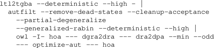
• $\texttt {Owl}\mathsf {IAR}^t$: Owl’s ltl2dra tool combined with optimized total-order $\mathsf {IAR}$ [21]

  

• $\texttt {Spot}\mathsf {IAR}^t$: Spot’s LTL to DRA translation combined with optimized total-order $\mathsf {IAR}$ [21]

  

• $\texttt {Owl}_{\text {\tiny LTL}}$: Owl’s ltl2dpa tool

  

• $\texttt {Spot}_{\text {\tiny LTL}}$: Spot’s LTL to DPA translation with some post-processing optimizations disabled

  

1.2 A.2 List of datasets

• dra2dpa: 100 randomly generated Rabin automata over 5 atomic propositions with 20 States, 6 Rabin pairs, a transition density of 5%, and acceptance probability of 10%. The set is simplified by both Owl’s and Spot’s automata optimizations.

  

• dra2dpa-large: 100 randomly generated Rabin automata over 5 atomic propositions with 20 States, 6 Rabin pairs, a transition density of 5%, and acceptance probability of 20%. The set is simplified by both Owl’s and Spot’s automata optimizations.

  

• ltl2dpa-rand: 100 randomly generated LTL formulae over 5 atomic propositions and Boolean size of 32–42. The set is simplified by both Owl’s and Spot’s LTL processing.

  

  Additional info on the bsize parameter, copied from Spot’s website:

  With --size the size of the formula is exactly the number of atomic propositions and operators used. [...] With --bsize, every Boolean subformula is counted as 1 in the total size. So F(a & b & c) would have Boolean-size 2. This type of size is probably a better way to classify formulas that are going to be translated as automata, since transitions are labelled by Boolean formulas: The complexity of the Boolean subformulas has little influence on the overall translation.

• ltl2dpa-lit: A collection of 165 formulae, obtained from several previous works [8, 11, 14, 31, 42, 43], simplified by both Owl and Spot. Since some contain duplicates (after simplification), the actual set only contains 155 formulae. All formulae are part of the artefact.

We note that both the configuration of the random generators as well as the selection of literature was done mostly arbitrary. We did not explicitly try to bias towards one particular tool. For the random datasets, we observed that runtimes etc. are very sensitive to changes of the random generator. We tried several combinations of parameters to obtain datasets where no tool exhausts the resources of reasonable consumer hardware, yet significant computation is performed. This arguably introduces a slight bias; however, when experimenting with larger datasets, similar patterns as the ones observed in Sect. 5 emerged. For the literature selection, we tried to avoid works for which one particular tool is known to have a significant advantage.

1.3 A.3 Comparisons for DRA-to-DPA translation

In this section, we present log-log-plots comparing the state count of selected pairs of tools on the set dra2dpa for the reader’s convenience. The solid and dashed lines indicate equal and double/half size, respectively. The artefact contains all pairwise comparisons.

1.4 A.4 Comparisons for LTL-to-DPA translation

As in the previous section, we provide log-log-plots for pairs of tools, showing the state-count on both the ltl2dpa-rand and ltl2dpa-lit separately.

1.4.1 A.4.1 ltl2dpa-rand comparison

1.4.2 A.4.2 ltl2dpa-lit comparison

References

Alur, R., La Torre, S.: Deterministic generators and games for LTL fragments. ACM Trans. Comput. Log. 5(1), 1–25 (2004). https://doi.org/10.1145/963927.963928
Babiak, T., Blahoudek, F., Kretínský, M., Strejcek, J.: Effective translation of LTL to deterministic Rabin automata: beyond the (F, G)-fragment. In: Automated Technology for Verification and Analysis—11th International Symposium, ATVA 2013, Hanoi, Vietnam, October 15–18, 2013. Proceedings, pp. 24–39 (2013). https://doi.org/10.1007/978-3-319-02444-8_4
Björklund, H., Sandberg, S., Vorobyov, S.: On fixed-parameter complexity of infinite games. In: The Nordic Workshop on Programming Theory (NWPT 2003), vol. 34, pp. 29–31. Citeseer (2003)
Büchi, J.R.: State-strategies for games in F G. J. Symb. Log. 48(4), 1171–1198 (1983). https://doi.org/10.2307/2273681
Casares, A., Colcombet, T., Fijalkow, N.: Optimal transformations of games and automata using Muller conditions. In: Bansal, N., Merelli, E., Worrell, J. (eds.) 48th International Colloquium on Automata, Languages, and Programming, ICALP 2021, July 12–16, 2021, Glasgow, Scotland (Virtual Conference), LIPIcs, vol. 198, pp. 123:1–123:14. Schloss Dagstuhl - Leibniz-Zentrum für Informatik (2021). https://doi.org/10.4230/LIPIcs.ICALP.2021.123
Chatterjee, K., Gaiser, A., Kretínský, J.: Automata with generalized Rabin pairs for probabilistic model checking and LTL synthesis. In: Sharygina, N., Veith, H. (eds.) Computer Aided Verification—25th International Conference, CAV 2013, Saint Petersburg, Russia, July 13–19, 2013. Proceedings, Lecture Notes in Computer Science, vol. 8044, pp. 559–575. Springer (2013). https://doi.org/10.1007/978-3-642-39799-8_37
Duret-Lutz, A., Lewkowicz, A., Fauchille, A., Michaud, T., Renault, E., Xu, L.: Spot 2.0—a framework for LTL and \(\omega \)-automata manipulation. In: Artho, C., Legay, A., Peled, D. (eds.) Automated Technology for Verification and Analysis—14th International Symposium, ATVA 2016, Chiba, Japan, October 17–20, 2016, Proceedings, Lecture Notes in Computer Science, vol. 9938, pp. 122–129 (2016). https://doi.org/10.1007/978-3-319-46520-3_8
Dwyer, M.B., Avrunin, G.S., Corbett, J.C.: Property specification patterns for finite-state verification. In: Ardis, M.A, Atlee, J.M. (eds.) Proceedings of the Second Workshop on Formal Methods in Software Practice, March 4–5, 1998, Clearwater Beach, Florida, USA, pp. 7–15. ACM (1998). https://doi.org/10.1145/298595.298598
Esparza, J., Kretínský, J., Sickert, S.: From LTL to deterministic automata—a safraless compositional approach. Form. Methods Syst. Des. 49(3), 219–271 (2016). https://doi.org/10.1007/s10703-016-0259-2
Esparza, J., Kretínský, J., Sickert, S.: One theorem to rule them all: a unified translation of LTL into \(\omega \)-automata. In: Dawar, A., Grädel, E. (eds.) Proceedings of the 33rd Annual ACM/IEEE Symposium on Logic in Computer Science, LICS 2018, Oxford, UK, July 09–12, 2018, pp. 384–393. ACM (2018). https://doi.org/10.1145/3209108.3209161
Etessami, K., Holzmann, G.J.: Optimizing Büchi automata. In: Palamidessi, C. (ed.) CONCUR 2000—Concurrency Theory, 11th International Conference, University Park, PA, USA, August 22–25, 2000, Proceedings, Lecture Notes in Computer Science, vol. 1877, pp. 153–167. Springer (2000). https://doi.org/10.1007/3-540-44618-4_13
Friedmann, O., Lange, M.: Solving parity games in practice. In: Automated Technology for Verification and Analysis, 7th International Symposium, ATVA 2009, Macao, China, October 14–16, 2009. Proceedings, pp. 182–196 (2009). https://doi.org/10.1007/978-3-642-04761-9_15
Gurevich, Y., Harrington, L.: Trees, automata, and games. In: Proceedings of the 14th Annual ACM Symposium on Theory of Computing, May 5–7, 1982, San Francisco, California, USA, pp. 60–65 (1982). https://doi.org/10.1145/800070.802177
Holeček, J., Kratochvíla, T., Řehák, V., Šafránek, D., Šimeček, P.: Verification Results in Liberouter Project (2004)
Klein, J., Baier, C.: Experiments with deterministic omega-automata for formulas of linear temporal logic. Theor. Comput. Sci. 363(2), 182–195 (2006). https://doi.org/10.1016/j.tcs.2006.07.022
Komárková, Z., Křetínský, J.: Rabinizer 3: safraless translation of LTL to small deterministic automata. In: Automated Technology for Verification and Analysis—12th International Symposium, ATVA 2014, Sydney, NSW, Australia, November 3–7, 2014, Proceedings, pp. 235–241 (2014). https://doi.org/10.1007/978-3-319-11936-6_17
Křetínský, J., Esparza, J.: Deterministic automata for the (F, G)-fragment of LTL. In: Computer Aided Verification—24th International Conference, CAV 2012, Berkeley, CA, USA, July 7–13, 2012 Proceedings, pp. 7–22 (2012). https://doi.org/10.1007/978-3-642-31424-7_7
Kretínský, J., Manta, A., Meggendorfer, T.: Semantic labelling and learning for parity game solving in LTL synthesis. In: Chen, Y., Cheng, C., Esparza, J. (eds.) Automated Technology for Verification and Analysis—17th International Symposium, ATVA 2019, Taipei, Taiwan, October 28–31, 2019, Proceedings, Lecture Notes in Computer Science, vol. 11781, pp. 404–422. Springer (2019). https://doi.org/10.1007/978-3-030-31784-3_24
Kretínský, J., Meggendorfer, T., Sickert, S.: Owl: a library for \(\omega \)-words, automata, and LTL. In: Lahiri, S.K., Wang, C. (eds.) Automated Technology for Verification and Analysis—16th International Symposium, ATVA 2018, Los Angeles, CA, USA, October 7–10, 2018, Proceedings, Lecture Notes in Computer Science, vol. 11138, pp. 543–550. Springer (2018). https://doi.org/10.1007/978-3-030-01090-4_34
Kretínský, J., Meggendorfer, T., Sickert, S., Ziegler, C.: Rabinizer 4: from LTL to your favourite deterministic automaton. In: Chockler, H., Weissenbacher, G. (eds.) Computer Aided Verification—30th International Conference, CAV 2018, Held as Part of the Federated Logic Conference, FloC 2018, Oxford, UK, July 14–17, 2018, Proceedings, Part I, Lecture Notes in Computer Science, vol. 10981, pp. 567–577. Springer (2018). https://doi.org/10.1007/978-3-319-96145-3_30
Kretínský, J., Meggendorfer, T., Waldmann, C., Weininger, M.: Index appearance record for transforming Rabin automata into parity automata. In: Legay, A., Margaria, T. (eds.) Tools and Algorithms for the Construction and Analysis of Systems—23rd International Conference, TACAS 2017, Held as Part of the European Joint Conferences on Theory and Practice of Software, ETAPS 2017, Uppsala, Sweden, April 22–29, 2017, Proceedings, Part I, Lecture Notes in Computer Science, vol. 10205, pp. 443–460 (2017). https://doi.org/10.1007/978-3-662-54577-5_26
Kupferman, O., Vardi, M.Y.: Safraless decision procedures. In: 46th Annual IEEE Symposium on Foundations of Computer Science (FOCS 2005), 23–25 October 2005, Pittsburgh, PA, SA, Proceedings, pp. 531–542 (2005). https://doi.org/10.1109/SFCS.2005.66
Löding, C.: Methods for the transformation of automata: complexity and connection to second order logic. Master’s thesis, Institute of Computer Science and Applied Mathematics, Christian-Albrechts-University of Kiel, Germany (1999)
Löding, C.: Optimal bounds for transformations of \(\omega \)-automata. In: Foundations of Software Technology and Theoretical Computer Science, 19th Conference, Chennai, India, December 13–15, 1999, Proceedings, pp. 97–109 (1999). https://doi.org/10.1007/3-540-46691-6_8
Löding, C., Tollkötter, A.: State space reduction for parity automata. In: Fernández, M., Muscholl, A. (eds.) 28th EACSL Annual Conference on Computer Science Logic, CSL 2020, January 13–16, 2020, Barcelona, Spain, LIPIcs, vol. 152, pp. 27:1–27:16. Schloss Dagstuhl - Leibniz-Zentrum für Informatik (2020). https://doi.org/10.4230/LIPIcs.CSL.2020.27
Luttenberger, M., Meyer, P., Sickert, S.: On the optimal and practical conversion of Emerson–Lei automata into parity automata. To appear (2021)
Meggendorfer, T.: Artefact for: index appearance record with preorders (2021). https://doi.org/10.5281/zenodo.4651156
Meyer, P.J., Luttenberger, M.: Solving mean-payoff games on the GPU. In: Artho, C., Legay, A., Peled, D. (eds.) Automated Technology for Verification and Analysis—14th International Symposium, ATVA 2016, Chiba, Japan, October 17–20, 2016, Proceedings, Lecture Notes in Computer Science, vol. 9938, pp. 262–267 (2016). https://doi.org/10.1007/978-3-319-46520-3_17
Mostowski, A.W.: Regular expressions for infinite trees and a standard form of automata. In: Skowron, A. (ed.) Computation Theory—Fifth Symposium, Zaborów, Poland, December 3–8, 1984, Proceedings, Lecture Notes in Computer Science, vol. 208, pp. 157–168. Springer (1984). https://doi.org/10.1007/3-540-16066-3_15
Muller, D.E.: Infinite sequences and finite machines. In: 4th Annual Symposium on Switching Circuit Theory and Logical Design, pp. 3–16. IEEE Computer Society, Chicago, Illinois, USA (1963). https://doi.org/10.1109/SWCT.1963.8
Pelánek, R.: BEEM: benchmarks for explicit model checkers. In: Bosnacki, D., Edelkamp, S. (eds.) Model Checking Software, 14th International SPIN Workshop, Berlin, Germany, July 1–3, 2007, Proceedings, Lecture Notes in Computer Science, vol. 4595, pp. 263–267. Springer (2007). https://doi.org/10.1007/978-3-540-73370-6_17
Piterman, N.: From nondeterministic Büchi and Streett automata to deterministic parity automata. In: 21th IEEE Symposium on Logic in Computer Science (LICS 2006), 12–15 August 2006, Seattle, WA, USA, Proceedings, pp. 255–264 (2006). https://doi.org/10.1109/LICS.2006.28
Piterman, N., Pnueli, A., Sa’ar, Y.: Synthesis of reactive(1) designs. In: Verification, Model Checking, and Abstract Interpretation, 7th International Conference, VMCAI 2006, Charleston, SC, USA, January 8–10, 2006, Proceedings, pp. 364–380 (2006). https://doi.org/10.1007/11609773_24
Pnueli, A.: The temporal logic of programs. In: 18th Annual Symposium on Foundations of Computer Science, Providence, Rhode Island, USA, 31 October–1 November 1977, pp. 46–57 (1977). https://doi.org/10.1109/SFCS.1977.32
Pnueli, A., Rosner, R.: On the synthesis of a reactive module. In: Conference Record of the Sixteenth Annual ACM Symposium on Principles of Programming Languages, Austin, Texas, USA, January 11–13, 1989, pp. 179–190 (1989). https://doi.org/10.1145/75277.75293
Rabin, M.O.: Decidability of second-order theories and automata on infinite trees. Trans. Am. Math. Soc. 141, 1–35 (1969)
Renkin, F., Duret-Lutz, A., Pommellet, A.: Practical “paritizing” of Emerson–Lei automata. In: Hung, D.V., Sokolsky, O. (eds.) Automated Technology for Verification and Analysis—18th International Symposium, ATVA 2020, Hanoi, Vietnam, October 19–23, 2020, Proceedings, Lecture Notes in Computer Science, vol. 12302, pp. 127–143. Springer (2020). https://doi.org/10.1007/978-3-030-59152-6_7
Safra, S.: On the complexity of \(\omega \)-automata. In: 29th Annual Symposium on Foundations of Computer Science, White Plains, New York, USA, 24–26 October 1988, pp. 319–327 (1988). https://doi.org/10.1109/SFCS.1988.21948
Safra, S.: Exponential determinization for \(\omega \)-automata with strong-fairness acceptance condition (extended abstract). In: Proceedings of the 24th Annual ACM Symposium on Theory of Computing, May 4–6, 1992, Victoria, British Columbia, Canada, pp. 275–282 (1992). https://doi.org/10.1145/129712.129739
Schewe, S.: Tighter bounds for the determinisation of Büchi automata. In: Foundations of Software Science and Computational Structures, 12th International Conference, FOSSACS 2009, Held as Part of the Joint European Conferences on Theory and Practice of Software, ETAPS 2009, York, UK, March 22–29, 2009. Proceedings, pp. 167–181 (2009). https://doi.org/10.1007/978-3-642-00596-1_13
Schwoon, S.: Determinization and complementation of Streett automata. In: Automata, Logics, and Infinite Games: A Guide to Current Research [Outcome of a Dagstuhl Seminar, February 2001], pp. 79–91 (2001). https://doi.org/10.1007/3-540-36387-4_5
Sickert, S., Esparza, J., Jaax, S., Kretínský, J.: Limit-deterministic Büchi automata for linear temporal logic. In: Chaudhuri, S., Farzan, A. (eds.) Computer Aided Verification—28th International Conference, CAV 2016, Toronto, ON, Canada, July 17–23, 2016, Proceedings, Part II, Lecture Notes in Computer Science, vol. 9780, pp. 312–332. Springer (2016). https://doi.org/10.1007/978-3-319-41540-6_17
Somenzi, F., Bloem, R.: Efficient Büchi automata from LTL formulae. In: Emerson, E.A., Sistla, A.P. (eds.) Computer Aided Verification, 12th International Conference, CAV 2000, Chicago, IL, USA, July 15–19, 2000, Proceedings, Lecture Notes in Computer Science, vol. 1855, pp. 248–263. Springer (2000). https://doi.org/10.1007/10722167_21
Streett, R.S.: Propositional dynamic logic of looping and converse is elementarily decidable. Inf. Control 54(1/2), 121–141 (1982). https://doi.org/10.1016/S0019-9958(82)91258-X
Tsai, M., Tsay, Y., Hwang, Y.: GOAL for games, omega-automata, and logics. In: Computer Aided Verification—25th International Conference, CAV 2013, Saint Petersburg, Russia, July 13–19, 2013. Proceedings, pp. 883–889 (2013). https://doi.org/10.1007/978-3-642-39799-8_62
Zielonka, W.: Infinite games on finitely coloured graphs with applications to automata on infinite trees. Theor. Comput. Sci. 200(1–2), 135–183 (1998). https://doi.org/10.1016/S0304-3975(98)00009-7
Open Access
This article is distributed under the terms of the Creative Commons Attribution 4.0 International License (http://creativecommons.org/licenses/by/4.0/), which permits unrestricted use, distribution, and reproduction in any medium, provided you give appropriate credit to the original author(s) and the source, provide a link to the Creative Commons license, and indicate if changes were made.
Funding
Open access funding provided by Institute of Science and Technology (IST Austria).
Author information
Authors and Affiliations
Corresponding author
Additional information
Publisher's Note
Springer Nature remains neutral with regard to jurisdictional claims in published maps and institutional affiliations.
This work is partially funded by the German Research Foundation (DFG) projects Verified Model Checkers (No. 317422601) and Statistical Unbounded Verification (No. 383882557), and the Alexander von Humboldt Foundation with funds from the German Federal Ministry of Education and Research. It is an extended version of [21], including all proofs together with further explanations and examples. Moreover, we provide a new, more efficient construction based on (total) preorders, unifying previous optimizations. Experiments are performed with a new, performant implementation, comparing our approach to the current state of the art.