Session-based concurrency, declaratively

Abstract

Session-based concurrency is a type-based approach to the analysis of message-passing programs. These programs may be specified in an operational or declarative style: the former defines how interactions are properly structured; the latter defines governing conditions for correct interactions. In this paper, we study rigorous relationships between operational and declarative models of session-based concurrency. We develop a correct encoding of session $\pi$-calculus processes into the linear concurrent constraint calculus ($\texttt {lcc}$), a declarative model of concurrency based on partial information (constraints). We exploit session types to ensure that our encoding satisfies precise correctness properties and that it offers a sound basis on which operational and declarative requirements can be jointly specified and reasoned about. We demonstrate the applicability of our results by using our encoding in the specification of realistic communication patterns with time and contextual information.

1 Introduction

This paper addresses the problem of relating two distinct models of concurrent processes: one of them, the session $\pi$-calculus [45] ($\pi$, in the following), is operational; the other one, the linear concurrent constraint calculus [22, 27] ($\texttt {lcc}$, in the following), is declarative. Our interest in these two models stems from the analysis of message-passing software systems, which are best specified by combining operational features (present in models such as $\pi$) and declarative features (present in models such as $\texttt {lcc}$). In this work, we aim at results of relative expressiveness, which explain how to faithfully encode programs in one model into programs in some other model [39, 40]. Concretely, we are interested in translations in which $\pi$ and $\texttt {lcc}$ are, respectively, source and target languages; a key common trait supporting expressiveness results between $\pi$ and $\texttt {lcc}$ is linearity, in the sense of Girard’s linear logic, the logic of consumable resources [24].

The process language $\pi$ falls within session-based concurrency, a type-based approach to the analysis of message-passing programs. In this approach, protocols are organized into basic units called sessions; interaction patterns are abstracted as session types [29], against which specifications may be checked. A session connects exactly two partners; session types ensure that interactions always occur in matching pairs: when one partner sends, the other receives; when one partner offers a selection, the other chooses; when a partner closes the session, the other acknowledges. When specifications are given in the $\pi$-calculus [33, 34], we obtain processes interacting along channels to implement session protocols. Sessions thus involve concurrency, mobility, and resource awareness: a session is a sequence of deterministic interactions on linear channels, to be used exactly once.

In specifying message-passing programs, operational and declarative features are complementary: while the former describe how a message-passing program is implemented, the latter describe what are the (least) conditions that govern a program’s correct behavior. Although languages based on the $\pi$-calculus can conveniently specify mobile, point-to-point communications, they do not satisfactorily express other kinds of requirements that influence protocol interactions and/or communicating partners—in particular, partial and contextual information can be unnatural or difficult to express in them.

To address this shortcoming, extensions of name-passing calculi such as, e.g., [5, 11, 14, 20, 21] have been developed: they typically add declarative features based on constraints (or assertions), i.e., logical conditions that specify and influence process behavior. Interestingly, several of these extensions are inspired by concurrent constraint programming [43] ($\texttt {ccp}$, in the following), a model of concurrency in which constraints (but also other forms of partial information) are a primitive concept. Process languages based on $\texttt {ccp}$ are appealing because they are simple, rest upon solid foundations, and are very expressive. Indeed, $\texttt {ccp}$ languages such as $\texttt {lcc}$ and $\texttt {utcc}$  [37] can represent mobility as in the $\pi$-calculus; such representations, however, tend to be unpractical for reasoning about message-passing programs.

In our view, this current state of affairs begs for a unifying account of operational and declarative approaches to session-based concurrency. We envision a declarative basis for session-based concurrency in which constructs from operational models (such as $\pi$) are given correct, low-level implementations in declarative models (such as $\texttt {lcc}$). Such implementations can then be freely used as “macros” in larger declarative specifications, in which requirements related to partial and contextual information can be cleanly expressed. In this way, existing operational and declarative languages (and their analysis techniques) can be articulated at appropriate abstraction levels. An indispensable step towards this vision is developing rigorous ways of compiling operational languages into declarative ones. This is the main technical challenge in this paper.

In line with this challenge, our previous work [31] formally related the session $\pi$-calculus in [29] and $\texttt {utcc}$ using an encoding, i.e., a language translation that satisfies certain encodability criteria [26]. Although this encoding already enables us to reason about message-passing specifications from a declarative standpoint, it presents some important limitations. First, the key rôle of linearity and type-based correctness in session-based concurrency is not explicit when encoding session $\pi$-calculus processes in $\texttt {utcc}$. Also, because $\texttt {utcc}$ is a deterministic language, the encoding in [31] can only translate deterministic session processes, and so it rules out useful forms of non-determinism that naturally arise in session-based concurrency.

To address these limitations within a unified account for session-based concurrency, here we develop an encoding of $\pi$ into $\texttt {lcc}$. Unlike $\texttt {utcc}$, $\texttt {lcc}$ treats constraints as linear resources that can be used exactly once. Our main discovery is that $\texttt {lcc}$ with its explicit treatment of linearity is a much better match for interactions in session-based concurrency than $\texttt {utcc}$. This is made formal by the tight correspondences between source processes in $\pi$ and target processes in $\texttt {lcc}$. Unlike $\texttt {utcc}$, $\texttt {lcc}$ is a non-deterministic language. Hence, by using $\texttt {lcc}$ as target language, our encoding can translate $\pi$ processes that cannot be translated by the encoding in [31], such as, e.g., a process specifying a session protocol in which a client can non-deterministically interact with multiple servers (cf. Ex. 3).

Summarizing, this paper develops the following contributions:

• A translation from $\pi$ into $\texttt {lcc}$ (Sect. 4). By using $\texttt {lcc}$ as target language, our translation supports linearity and non-determinism, as essential in session-based concurrency.

• A study of the conditions under which the session types by Vasconcelos [45] enable us to correctly translate $\pi$ processes into $\texttt {lcc}$ (Sect. 3.1). We use these conditions to prove that our translation is a valid encoding: it satisfies Gorla’s encodability criteria [26], in particular operational correspondence.

• Extended examples that showcase how processes resulting from our encoding can be used as macros in declarative specifications (Sect. 5). By exploiting a general strategy that uses encoded processes as code snippets, we specify in $\texttt {lcc}$ two of the communication patterns with time in [36].

The rest of this paper is structured as follows. Section 2 describes session-based concurrency and introduces the key ideas in our approach. Section 3 presents required background on relative expressiveness, $\pi$, and $\texttt {lcc}$. In particular, Sect. 3.1 presents a variant of the session types in [45] that is crucial to establish correctness for our translation. Section 4 presents the translation of $\pi$ into $\texttt {lcc}$ and establishes its correctness. Section 5 develops the extended examples. We close by discussing related work (Sect. 6) and giving some concluding remarks (Sect. 7). “Appendices” contain additional examples and omitted proofs.

This paper builds upon results first reported in the conference paper [17]. Such results include (i) an encoding of $\pi$ into $\texttt {lcc}$, as well as (ii) an encoding of an extension of $\pi$ with session establishment into a variant of $\texttt {lcc}$. Here, we offer a revised, extended presentation of the results on (i), for which we present stronger correspondences, full technical details, and additional examples. This focus allows us to keep presentation compact; a detailed description of the results related to (ii) can be found in Cano’s PhD thesis [15].

2 Overview of key ideas

We informally illustrate our approach and main results. We use $\pi$ and $\texttt {lcc}$ processes, whose precise syntax and semantics will be introduced in the following section.

Session-Based Concurrency. Consider a simple protocol between a client and a shop:

• 1. The client sends a description of an item that she wishes to buy to the shop.

• 2. The shop replies with the price of the item and offers two options to the client: to buy the item or to close the transaction.

• 3. Depending on the price, the client may choose to purchase the item or to end the transaction.

Here is a session type that specifies this protocol from the client’s perspective:

$$\begin{aligned} S =~ !\mathsf {item}.\,?\mathsf {price}.\,\oplus \{{\textit{buy}}:\,!\mathsf {ccard}.\,?\mathsf {invoice}.\,\texttt {end}\, , \,{\textit{quit}}:\,!\mathsf {bye}.\,\texttt {end}\} \end{aligned}$$

Type S says that the output of a value of type $\mathsf {item}$ (denoted $!\mathsf {item}$) should be followed by the input of a value of type $\mathsf {price}$ (denoted $?\mathsf {price}$). These two actions should precede the selection (internal choice, denoted $\oplus$) between two different behaviors distinguished by labels ${\textit{buy}}$ and ${\textit{quit}}$: in the first behavior, the client sends a value of type $\mathsf {ccard}$, then receives a value of type $\mathsf {invoice}$, and then closes the protocol ($\texttt {end}$ denotes the concluded protocol); in the second behavior, the client emits a value of type $\mathsf {bye}$ and closes the session.

From the shop’s perspective, we would expect a protocol that is complementary to S:

$$ \begin{aligned} T =~ ?\,\mathsf {item}.\,!\mathsf {price}.\, \& \{{\textit{buy}}:\,?\mathsf {ccard}.\,!\mathsf {invoice}.\,\texttt {end}\, , \,{\textit{quit}}:\,?\mathsf {bye}.\,\texttt {end}\} \end{aligned}$$

After receiving a value of type $\mathsf {item}$, the shop sends a value of type $\mathsf {price}$ back to the client. Using external choice (denoted&), the shop then offers two behaviors to the client, identified by labels ${\textit{buy}}$ and ${\textit{quit}}$. The complementarity between types such as S and T is formalized by session-type duality (see, e.g., [23]). The intent is that implementations derived from dual session types will respect their (complementary) protocols at run-time, avoiding communication mismatches and other insidious errors.

We illustrate the way in which session types relate to $\pi$ processes. We write ${x}\langle v\rangle .P$ and x(y).P to denote output and input along name x, with continuation P. Also, given a finite set I, we write $x \triangleright \{{\textit{lab}}_i:P_i\}_{i\in I}$ to denote the offer of labeled processes $P_1, P_2, \ldots$ along name x; dually, $x \triangleleft {\textit{lab}}.\,P$ denotes the selection of a label ${\textit{lab}}$ along x. Moreover, process $b?\,P\!:\!Q$ denotes a conditional expression which executes P or Q depending on Boolean b. Process $P_x$ below is a possible implementation of type S along x:

$$\begin{aligned} P_x&= {x}\langle \mathsf {book}\rangle .\,x(z).\,(z \le 20)?\,x \triangleleft {\textit{buy}}.\,{x}\langle 5406\rangle .\,x(inv).\mathbf {0} \!:\!x \triangleleft {\textit{quit}}. \,{x}\langle {\textit{end}}\rangle .\,{\mathbf {0} } \end{aligned}$$

(1)

$$\begin{aligned} P_y&= y(w). {y}\langle \mathsf {price}(w)\rangle .y \triangleright \{{\textit{buy}}:y(w').{y}\langle \mathsf {invoice} \rangle .\mathbf {0} , {\textit{quit}}:y(w''). \mathbf {0} \} \end{aligned}$$

(2)

Process $P_x$ uses a conditional to implement the decision of which option offered by the shop is chosen: the purchase will take place only if the item (a book) is within a $20 budget. We assume that ${\textit{end}}$ is a value of type $\mathsf {bye}$. Similarly, $P_y$ is a process that implements the shop’s intended protocol along y: it first expects a petition for an item (w), and after that returns the item’s current price. Then, it offers the buyer a (labeled) choice: either to buy the item or to quit the transaction.

Sessions with Declarative Conditions. The session-based calculus $\pi$ is a language with point-to-point, synchronous communication. Hence, $\pi$ processes can appropriately describe protocol actions, but can be less adequate to express contextual conditions on partners and their interactions, which are usually hard to know and predict. Consider a variation of the above protocol, in which the last step is specified as follows:

• 3’. Depending on the item’s price and whether the purchase occurs in a given time interval (say, a discount period), the client may either purchase the item or end the transaction.

This kind of time constraints has been studied in [36], where a number of timed patterns in communication protocols are identified and analyzed. These patterns add flexibility to specifications by describing the protocol’s behavior with respect to external sources (e.g., non-interacting components like clocks and the communication infrastructure). For example, a protocol step such as 3’ dictates that communication actions will be executed only within a given time interval. Hence, even though timed requirements do not necessarily enact a communicating action, they may influence interactions between partners.

Timed patterns are instances of declarative requirements, which are difficult to express in the (session) $\pi$-calculus. Formalizing Step 3’ in $\pi$ is not trivial, because one must necessarily represent time units by using synchronizations—a far-fetched relationship. The (session) $\pi$-calculus does not naturally lend itself to specify the combination of operational descriptions of structured interactions (typical of sessions) and declarative requirements (as in, e.g., protocol and workflow specifications). Given this, our aim is to use $\texttt {lcc}$ as a unified basis for both operational and declarative requirements in session-based concurrency.

$\texttt {ccp}$ and $\texttt {lcc}$. $\texttt {lcc}$ is based on concurrent constraint programming ($\texttt {ccp}$) [43]. In $\texttt {ccp}$, processes interact via a constraint store (store, in the sequel) by means of tell and ask operations. Processes may add constraints (pieces of partial information) to the store via tell operations; using ask operations processes may query the store about some constraint and, depending on the result of the query, execute a process or suspend. These queries are governed by a constraint system, a parametric structure that specifies the entailment relation between constraints. The constraint store thus defines an asynchronous synchronization mechanism; both communication-based and external events can be modeled as constraints in the store.

In $\texttt {lcc}$, tell and ask operations work as follows. Let c and d denote constraints, and let $\widetilde{x}$ denote a (possibly empty) vector of variables. While the tell process $\overline{c}$ can be seen as the output of c to the store, the parametric ask operator $\mathbf {\forall }{\widetilde{x}}(d \!\rightarrow \! P)$ may be read as: if d can be inferred from the store, then P will be executed; hence, P depends on the guard d. These parametric ask operators are called abstractions. Resource awareness in $\texttt {lcc}$ is crucial: not only the inference consumes the abstraction (i.e., it is linear), it may also involve the consumption of constraints in the store as well as substitution of parameters $\widetilde{x}$ in P.

In $\texttt {lcc}$, parametric asks can express name mobility as in the $\pi$-calculus [27, 44]. That is, the key operational mechanisms of the (session) $\pi$-calculus (name communication, scope extrusion) admit (low-level) declarative representations as $\texttt {lcc}$ processes.

Our Encoding To illustrate our encoding, let us consider the most elementary computation step in $\pi$, which is given by the following reduction rule:

where v is a value or a variable. This rule specifies the synchronous communication between two complementary (session) endpoints, represented by the output process ${x}\langle v\rangle .P$ and the input process y(z).Q. In session-based concurrency, no races in communications between endpoints can occur. We write $(\varvec{\nu }xy) P$ to denote that (bound) variables x and y are reciprocal endpoints for the same session protocol in P.

Our encoding $\llbracket \cdot \rrbracket$ translates $\pi$ processes into $\texttt {lcc}$ processes (cf. Fig. 8). The essence of this declarative interpretation is already manifest in the translation of output- and input-prefixed processes:

$$\begin{aligned} \llbracket {x}\langle v\rangle .P \rrbracket&= \overline{\mathsf {snd} (x,v)} \parallel \mathbf {\forall }{z}\big (\mathsf {rcv} (z,v)\otimes \{x{:}z\} \rightarrow \llbracket P \rrbracket \big ) \\ \llbracket x(y).Q \rrbracket&= \mathbf {\forall }{y,w}\big (\mathsf {snd} (w,y)\otimes \{w{:}x\} \rightarrow \overline{\mathsf {rcv} (x,y)} \parallel \llbracket Q \rrbracket \big ) \end{aligned}$$

where $\otimes$ denotes multiplicative conjunction in linear logic. We use predicates $\mathsf {snd} (x,v)$ and $\mathsf {rcv} (x,y)$ to represent synchronous communication in $\pi$ using the asynchronous communication model of $\texttt {lcc}$; also, we use the constraint $\{x{:}z\}$ to indicate that x and z are dual endpoints. These pieces of information are treated as linear resources by $\texttt {lcc}$; this is key to ensure operational correspondence (cf. Theorems 11 and 12). As we will see, $\llbracket {x}\langle v\rangle .P \rrbracket$ and $\llbracket x(y).Q \rrbracket$ synchronize in two steps. First, constraint $\mathsf {snd} (x,v)$ is consumed by the abstraction in $\llbracket x(y).Q \rrbracket$, thus enabling $\llbracket Q \rrbracket$ and adding $\mathsf {rcv} (x,y)$ to the store. Then, constraint $\mathsf {rcv} (x,y)$ is consumed by the abstraction $\mathbf {\forall }{z}\big (\mathsf {rcv} (z,v)\otimes \{x{:}z\} \rightarrow \llbracket P \rrbracket \big )$, thus enabling $\llbracket P \rrbracket$.

Encoding Correctness using Session Types. To contrast the rôle of linearity in $\pi$ and in $\texttt {lcc}$, we focus on $\pi$ processes which are well-typed in the type system by Vasconcelos [45]. Type soundness in [45] ensures that well-typed processes never reduce to ill-formed processes that do not respect their intended session protocols.

The type system in [45] offers flexible support for processes with infinite behavior, in the form of recursive session types that can be shared among multiple threads. Using recursive session types, the type system in [45] admits $\pi$ processes with output races, i.e., processes in which two or more sub-processes in parallel have output actions on the same variable. Here is a simple example of a process with an output race (on x), which is typable in [45]:

$$\begin{aligned} R_1 = (\varvec{\nu }xy)({x}\langle v_1\rangle .Q_1 \mathord {\;|\;}{x}\langle v_2\rangle .Q_2 \mathord {\;|\;}\mathbf {*}\, y(z).Q_3) \end{aligned}$$

(3)

Even though our translation $\llbracket \cdot \rrbracket$ works fine for the set of well-typed $\pi$ processes as defined in [45], the class of typed processes with output races represents a challenge for proving that the translation $\llbracket \cdot \rrbracket$ is correct. We aim at correctness in the sense of Gorla’s encodability criteria [26], which define a general and widely used framework for studying relative expressiveness. Roughly speaking, $\pi$ processes with output races induce ambiguities in the $\texttt {lcc}$ processes that are obtained via $\llbracket \cdot \rrbracket$. To illustrate this, consider the translation of $R_1$:

$$\begin{aligned} \begin{aligned} \llbracket R_1 \rrbracket =~&C[\overline{\mathsf {snd} (x,v_1)} \parallel \mathbf {\forall }{w_1}\big (\mathsf {rcv} (w_1,v_1)\otimes \{x{:}w_1\} \rightarrow \llbracket Q_1 \rrbracket \big ) \parallel \\&\quad \overline{\mathsf {snd} (x,v_2)} \parallel \mathbf {\forall }{w_2}\big (\mathsf {rcv} (w_2,v_2)\otimes \{x{:}w_2\} \rightarrow \llbracket Q_2 \rrbracket \big ) \parallel \\&\quad {{\,\mathrm{!}\,}}\mathbf {\forall }{z,w_3}\big (\mathsf {snd} (w_3,z)\otimes \{w_3{:}y\} \rightarrow \overline{\mathsf {rcv} (y,z)} \parallel \llbracket Q_3 \rrbracket \big ) ] \end{aligned} \end{aligned}$$

where context $C[-]$ includes the constraints needed for interaction (i.e., $\{x{:}y\}$) and ‘${{\,\mathrm{!}\,}}$’ denotes replication. The ambiguities concern the values involved as objects in the output races. If we assume $v_1 \ne v_2$, then there are no ambiguities and translation correctness as in [26] can be established. Now, if $v_1 = v_2$ then $\mathsf {snd} (x,v_1) = \mathsf {snd} (x,v_2)$, which is problematic for translation correctness (in particular, for proving operational correspondence): once process ${{\,\mathrm{!}\,}}\mathbf {\forall }{z,w_3}\big (\mathsf {snd} (w_3,z)\otimes \{w_3{:}y\} \rightarrow \overline{\mathsf {rcv} (y,z)} \parallel \llbracket Q_3 \rrbracket \big )$ consumes either constraint, we cannot precisely determine which continuation should be enabled with constraint $\mathsf {rcv} (x,v_i)$—both $\llbracket Q_1 \rrbracket$ and $\llbracket Q_2 \rrbracket$ could be spawned at that point.

To establish translation correctness following the criteria in [26], we narrow down the class of typable $\pi$ processes in [45] by disallowing processes with output races. To this end, we introduce a type system in which a recursive type involving an output behavior (a potential output race) can be associated to at most one thread. This is a conservative solution, which allows us to retain useful forms of infinite behavior. Although process $R_1$ in (3) is not typable in our type system, it allows processes such as

$$\begin{aligned} (\varvec{\nu }xy)({x}\langle v_1\rangle . {x}\langle v_2\rangle .Q_1 \mathord {\;|\;}\mathbf {*}\, y(z).Q_2) \end{aligned}$$

in which the parallel server invocations exhibited by $R_1$ have been sequentialized.

3 Preliminaries

We start by introducing the source and target languages (Sects. 3.1 and 3.2) and the encodability criteria we shall use as reference for establishing translation correctness (Sect. 3.3).

3.1 A session $\pi$-calculus without output races ($\pi$)

We present the session $\pi$-calculus ($\pi$) and its associated type system, a specialization of that by Vasconcelos [45] that disallows output races.

3.1.1 Syntax and semantics

We assume a countably infinite set of variables $\mathcal {V}_{\pi }$, ranged over by $x, y, \ldots$. Channels are represented as pairs of variables, called covariables. Messages are represented by values, ranged over by $v,v',u,u',\ldots$ and whose base set is called $\mathcal {U}_{\pi }$. Values can be both variables and the Boolean constants $\texttt {tt} , \texttt {ff}$. We also use $l, l', \ldots$ to range over a countably infinite set of labels, denoted $\mathcal {B}_\pi$. We write $\widetilde{x}$ to denote a finite sequence of variables $x_1,\ldots ,x_n$ with $n\ge 0$ (and similarly for other elements).

Definition 1

($\pi$) The set of $\pi$ processes is defined by grammar below:

$$\begin{aligned} \begin{aligned} P,Q&{:}{:}=~ {x}\langle v\rangle .P \, {\big |}\,x(y).P \, {\big |}\,x \triangleleft l.P\, {\big |}\,x \triangleright \{l_i:P_i\}_{i\in I} \, {\big |}\,b?\,P\!:\!Q \, {\big |}\,\mathbf {*}\, x(y).P\\&\, {\big |}\,(\varvec{\nu }xy)P \, {\big |}\,P \,|\, Q \, {\big |}\,\mathbf {0} \end{aligned} \end{aligned}$$

Process ${x}\langle v\rangle .P$ sends value v over x and then continues as P; dually, process x(y).Q expects a value v on x that will replace all free occurrences of y in Q. Processes $x \triangleleft l_j.P$ and $x \triangleright \{l_i:Q_i\}_{i\in I}$ define a labeled choice mechanism, with labels indexed by the finite set I: given $j \in I$, the selection process $x \triangleleft l_j.P$ uses x to select $l_j$ from the branching process $x \triangleright \{l_i:Q_i\}_{i\in I}$, thus triggering process $Q_j$. We assume pairwise distinct labels. The conditional process $v?\,P\!:\!Q$ behaves as P if v evaluates to $\texttt {tt}$; otherwise it behaves as Q. Process $\mathbf {*}\, x(y).P$ denotes a replicated input process, which allows us to specify persistent servers. The restriction $(\varvec{\nu }xy)P$ binds together x and y in P, thus indicating that they are two endpoints of the same channel (i.e., the same session). Processes for parallel composition $P \, {\mid }\,Q$ and inaction $\mathbf {0}$ are standard.

We write $(\varvec{\nu }\widetilde{x}\widetilde{y})P$ to stand for $(\varvec{\nu }x_1,\ldots ,x_n \, y_1,\ldots ,y_n)P$, for some $n\ge 1$. We often write $\prod _{i = 1}^{n}P_i$ to stand for $P_1 \, {\mid }\,\cdots \, {\mid }\,P_n$, and refer to the parallel sub-processes of $P_1, \ldots , P_n$ as threads.

In x(y).P and $\mathbf {*}\, x(y).P$ (resp. $(\varvec{\nu }yz)P$) occurrences of y (resp. y, z) are bound with scope P. The set of free variables of P, denoted $\mathsf {fv}_{\pi }(P)$, is standardly defined.

Fig. 1

Reduction relation for $\pi$ processes

Remark 1

(Barendregt’s variable convention) Throughout the paper, in both $\pi$ and $\texttt {lcc}$, we shall work up to $\alpha$-equivalence, as usual; in definitions and proofs we assume that all bound variables are distinct from each other and from all free variables.

The operational semantics for $\pi$ is given as a reduction relation $\longrightarrow$, the smallest relation generated by the rules in Fig. 1. Reduction expresses the computation steps that a process performs on its own. It relies on a structural congruence on processes, given below.

Definition 2

(Structural Congruence) The structural congruence relation for $\pi$ processes is the smallest congruence relation $\equiv _{\pi }$ that satisfies the following axioms and identifies processes up to renaming of bound variables (i.e., $\alpha$-conversion, denoted $\equiv _\alpha$).

Intuitions on the rules in Fig. 1 follow. Reduction requires an enclosing restriction $(\varvec{\nu }xy)(\,\cdots )$; this represents that a session connecting endpoints x and y has been already established. Hence, communication cannot occur on free variables, as there is no way to tell what is the pair of interacting covariables. In Rules ${\lfloor \textsc {Com}\rfloor }$, ${\lfloor \textsc {Sel}\rfloor }$, and ${\lfloor \textsc {Rep}\rfloor }$, the restriction is persistent after each reduction, to allow further synchronizations on x and y. In the same rules, process R stands for all the threads that may share x and y.

Rule ${\lfloor \textsc {Com}\rfloor }$ represents the synchronous communication of value v through endpoint x to endpoint y. Furthermore, Rule ${\lfloor \textsc {Sel}\rfloor }$ formalizes a labeled choice mechanism, in which communication of a label $l_j$ is used to choose which of the $Q_i$ will be executed, Rule ${\lfloor \textsc {Rep}\rfloor }$ is similar to Rule ${\lfloor \textsc {Com}\rfloor }$, and used to spawn a new copy of Q, available as a replicated server. Rules ${\lfloor \textsc {IfT}\rfloor }$ and ${\lfloor \textsc {IfF}\rfloor }$ are self-explanatory. Rules for reduction within parallel and restriction contexts, together with reduction up to $\equiv _{\pi }$, are standard.

To reason compositionally about the syntactic structure of processes, we introduce (evaluation) contexts. A context represents a process with a “hole”, denoted ‘$-$’, which may be filled by another process.

Definition 3

(Contexts for $\pi$) The syntax of (evaluation) contexts in $\pi$ is given by the following grammar:

$$\begin{aligned} E {:}{:}= - ~\mathord {\,\big |\,}~ E \, {\mid }\,P ~\mathord {\,\big |\,}~ P \, {\mid }\,E ~\mathord {\,\big |\,}~ (\varvec{\nu }xy)(E) \end{aligned}$$

where P is a $\pi$ process. We write $C[- ]$ to range over contexts of the form $(\varvec{\nu }\widetilde{x}\widetilde{y})(-)$. Also, we write $E[P ]$ (resp. $C[P ]$) to denote the process obtained by filling ‘$-$’ with P.

3.1.2 Type system

We now present the type system for $\pi$, a variant of the system in [45]. Rem. 2 discusses the differences of our type system with respect to the one in [45].

We use $q, q',\dots$, to range over qualifiers; $p, p' ,\dots$, to range over pre-types; $T,U,\dots$ to range over types, and $\varGamma , \varGamma ',\dots$ to range over the typing contexts which gather assignments of the form x : T, where x is a variable and T is a type. As usual, we treat contexts up to the exchange of entries; the variables that appear in a context are required to be pairwise distinct. The concatenation of typing contexts $\varGamma _1$ and $\varGamma _2$ is written $\varGamma _1, \varGamma _2$.

Definition 4

(Syntax of Types) The syntax of types and typing contexts is in Fig. 2.

Fig. 2

Session types: qualifiers, pre-types, types, and typing contexts

Intuitively, pre-types represent pure communication behavior (e.g., send, receive, selection, and branching). Pre-type $!T_1.T_2$ represents a protocol that sends a value of type $T_1$ and then continues according to type $T_2$. Dually, pre-type $?T_1.T_2$ represents a protocol that receives a value of type $T_1$ and then proceeds according to type $T_2$. Pre-types $\oplus \{l_i:T_i\}_{i\in I}$ and&$\{l_i:T_i\}_{i\in I}$ denote labeled selection (internal choice) and branching (external choice), respectively.

Pre-types are given a qualifier q to indicate whether the communication behavior is unrestricted or linear. Linearly qualified pre-types can only be assigned to variables that do not appear shared among threads, whereas unrestricted pre-types may be assigned to variables shared among different threads.

Types can be one of the following: (1) $\texttt {bool}$, used for constants and variables; (2) $\texttt {end}$, which indicates a terminated behavior; (3) qualified pre-types; or (4) recursive types for disciplining potentially infinite communication patterns. Recursive types are considered equi-recursive (i.e., a recursive type and its unfolding are considered equal because they represent the same regular infinite tree) and contractive (i.e., containing no sub-expression of the form $\mu \mathsf {a}_1.\cdots .\mu \mathsf {a}_n.\mathsf {a}_1$) [42]. The qualifier of a recursive type $T = \mu \mathsf {a}. T'$ is obtained via unfolding and by assigning the qualifier of the body $T'$ to type T.

As in [45], we omit $\texttt {end}$ at the end of types whenever it is not needed; we also write recursive types $\mu \mathsf {a}. {{\,\mathrm{\texttt {un}}\,}}!T.\mathsf {a}$ and $\mu \mathsf {a}. {{\,\mathrm{\texttt {un}}\,}}?T.\mathsf {a}$ as $\mathbf {*}\,!T$ and $\mathbf {*}\,?T$, respectively.

We use predicates over types to control which types can be shared among variables. While in [45] all unrestricted types can be shared, we proceed differently: to rule out output races, we enforce that only unrestricted input-like types can be shared. We start by presenting an auxiliary predicate that allows us to distinguish output-like types—even when the output behavior in the type is not immediate:

Definition 5

(Output-Like Unrestricted Types) We define the predicate $\texttt {out}(p)$ on pre-types inductively:

$$ \begin{aligned} \texttt {out}(!T.U)&{\mathop {=}\limits ^{\texttt {def} }} \texttt {tt}&\texttt {out}(?T.U)&{\mathop {=}\limits ^{\texttt {def} }} \texttt {out}(U) \\ \texttt {out}(\oplus \{l_i:T_i\}_{i\in I} )&{\mathop {=}\limits ^{\texttt {def} }} \texttt {tt}&\texttt {out}( \& \{l_i:T_i\}_{i\in I})&{\mathop {=}\limits ^{\texttt {def} }} \bigvee _{i\in I} \texttt {out}(T_i) \end{aligned}$$

The predicate is lifted to types as follows:

$$\begin{aligned} \texttt {out}(\texttt {bool})&{\mathop {=}\limits ^{\texttt {def} }} \texttt {ff}&\texttt {out}(\texttt {end})&{\mathop {=}\limits ^{\texttt {def} }} \texttt {ff}&\texttt {out}(\mathsf {a})&{\mathop {=}\limits ^{\texttt {def} }} \texttt {ff}\\ \texttt {out}(qp)&{\mathop {=}\limits ^{\texttt {def} }} \texttt {out}(p)&\texttt {out}(\mu \mathsf {a}. T)&{\mathop {=}\limits ^{\texttt {def} }} \texttt {out}(T) \end{aligned}$$

Using this predicate, we have the following definition, which specializes the one in [45]:

Definition 6

(Predicates for Types and Contexts) Let T be a session type (cf. Fig. 2). We define $\texttt {un}^{\star }(T)$ as follows:

• $\texttt {un}^{\star }(T)$ if and only if $(T = \texttt {bool}) \vee (T = \texttt {end}) \vee (T = {{\,\mathrm{\texttt {un}}\,}}p \wedge \lnot \texttt {out}(p))$.

Also, we define $\texttt {un}^{\star }(\varGamma )$ if and only if $x:T \in \varGamma$ implies $\texttt {un}^{\star }(T)$.

Above, predicate $\texttt {un}^{\star }(T)$ modifies the $\texttt {un}(T)$ predicate in [45] to rule out the sharing of output-like types: it requires that pre-types qualified with ‘${{\,\mathrm{\texttt {un}}\,}}$’ do not satisfy $\texttt {out}(\cdot )$.

Session-type systems use duality to relate types with complementary (or opposite) behaviors: e.g., the dual of input is output (and vice versa); branching is the dual of selection (and vice versa). We define duality by induction on the structure of types.

Definition 7

(Duality of Session Types) For every type T except $\texttt {bool}$, we define its dual $\overline{T}$ inductively:

$$ \begin{aligned} \overline{\texttt {end}} {\mathop {=}\limits ^{\texttt {def} }} \texttt {end}\qquad \overline{\mathsf {a}} {\mathop {=}\limits ^{\texttt {def} }} \mathsf {a} \qquad \overline{!T.U}\,\, {\mathop {=}\limits ^{\texttt {def} }} \,\, ?T.\overline{U} \qquad \overline{?T.U}\,\, {\mathop {=}\limits ^{\texttt {def} }} \,\, !T.\overline{U} \\ \overline{\!\oplus \!\{l_i:T_i\}_{i\in I}} {\mathop {=}\limits ^{\texttt {def} }} \! \& \!\{l_i:\overline{T_i}\}_{i\in I} \qquad \overline{\! \& \!\{l_i:T_i\}_{i\in I}} {\mathop {=}\limits ^{\texttt {def} }} \!\oplus \!\{l_i:\overline{T_i}\}_{i\in I} \qquad \overline{\mu \mathsf {a}. T} {\mathop {=}\limits ^{\texttt {def} }} \mu \mathsf {a}. \overline{T} \end{aligned}$$

Duality in the presence of recursive types is delicate [7]. While intuitive, the inductive definition above is correct only for tail recursive types, in which all message types are closed. To account also for non-tail-recursive types (e.g., $\mu \mathsf {a}. ?\mathsf {a}.\mathsf {a}$) a more involved coinductive definition is required, cf. Definition 37 in “Appendix”. The reader is referred to [23] for a detailed treatment of duality, where Definition 7 is called “naive duality”. Notice that using naive duality does not undermine the correctness of our results.

We shall use a splitting operator on typing contexts, denoted ‘$\circ$’, to maintain the linearity invariant for variables on typing derivations. Because of predicate $\texttt {un}^{\star }(\cdot )$ the splitting operation will not allow to share unrestricted output-like types.

Definition 8

(Typing Context Splitting) Let $\varGamma _1$ and $\varGamma _2$ be two typing contexts. The (typing) context splitting of $\varGamma _1$ and $\varGamma _2$, written $\varGamma _1 \circ \varGamma _2$, is defined as follows:

We also define a ‘$+$’ operation to correctly update typing contexts during derivations:

There are two typing judgments. We write $\varGamma \vdash v:T$ to denote that value v has type T under $\varGamma$. Also, we write $\varGamma \vdash P$ to denote that process P is well-typed under $\varGamma$.

Fig. 3

Session types: typing rules for $\pi$ processes

Figure 3 gives the typing rules for constants, variables, and processes; some intuitions follow. Rules ${(\textsc {T:Bool})}$ and ${(\textsc {T:Var})}$ are for variables; in both cases, we require $\texttt {un}^{\star }(\varGamma )$ to ensure that all variables assigned to types that do not satisfy predicate $\texttt {un}^{\star }(\cdot )$ are consumed. Rule ${(\textsc {T:In})}$ types an input process: it checks whether x has the right type and checks the continuation; it also adds variable y with type T and updates x in $\varGamma$ with type U. To type-check a process ${x}\langle v\rangle .P$, Rule ${(\textsc {T:Out})}$ splits the typing context in three parts: the first checks the type of the subject x; the second checks the type of the object v; the third checks the continuation P. Rules ${(\textsc {T:Sel})}$ and ${(\textsc {T:Bra})}$ type-check selection and branching processes, and work similarly to Rules ${(\textsc {T:Out})}$ and ${(\textsc {T:In})}$, respectively.

Rule ${(\textsc {T:Rin})}$ types a replicated input $\mathbf {*}\, x(y).P$ under the context $\varGamma$; it presents several differences with respect to the rule in [45]. Our rule requires $\varGamma$ to satisfy predicate $\texttt {un}^{\star }(\cdot )$. Also, the type T of y must either satisfy $\texttt {un}^{\star }(\cdot )$ or be linear. The rule also requires that $\varGamma$ assigns x an input type qualified with ${{\,\mathrm{\texttt {un}}\,}}{}$, and that the continuation P is typed with a context that contains y : T and x : U.

Rule ${(\textsc {T:Par})}$ types parallel composition using the (context) splitting operation to divide resources among the two threads. Rule ${(\textsc {T:Res})}$ types the restriction operator by performing a duality check on the types of the covariables. Rule ${(\textsc {T:If})}$ type-checks the conditional process. Given the inactive process $\mathbf {0}$, Rule ${(\textsc {T:Nil})}$ checks that the context satisfies $\texttt {un}^{\star }(\cdot )$ and Rule ${(\textsc {T:WkNil})}$ ensures that unrestricted types that are output-like (cf. Definition 5) can be weakened when needed. The following example illustrates the need for this rule:

Example 1

(Recursive Types and Rule ${(\textsc {T:WkNil})}$) We show the kind of recursive processes typable in our system, and the most glaring differences with respect to [45]. Process $P_1 = {x}\langle \texttt {tt} \rangle .{x}\langle \texttt {ff} \rangle .\mathbf {0}$ is typable both in our system and in the one in [45] under a context in which x is assigned the recursive type $T = \mu \mathsf {a}. {{\,\mathrm{\texttt {un}}\,}}!\texttt {bool}.\mathsf {a}$. Let us consider the typing derivation for $P_1$ in our system:

Notice that, by Definition 6, $\texttt {un}^{\star }(T)$ does not hold because $\texttt {out}(T)$ holds. This in turn influences the context splitting (Definition 8) required by Rule ${(\textsc {T:Out})}$: the assignment x : T can only appear in one of the branches of the split (the middle one). Let us consider U and D, which appear unspecified above. Because we use equi-recursive types (as in [45]), T is equivalent to $U = {!}\texttt {bool}.\mu \mathsf {a}. {{\,\mathrm{\texttt {un}}\,}}!\texttt {bool}.\mathsf {a}$, which means that the judgment in the rightmost branch becomes $x: T \vdash {x}\langle \texttt {ff} \rangle .\mathbf {0}$. To determine its derivation D, we use Rule ${(\textsc {T:WkNil})}$:

Indeed, before concluding the derivation for the rightmost branch, we are left with the judgment $x: T \vdash \mathbf {0}$. Because $\texttt {un}^{\star }(T)$ does not hold, we cannot apply Rule ${(\textsc {T:Nil})}$: to complete the derivation, we first apply Rule ${(\textsc {T:WkNil})}$ and then apply Rule ${(\textsc {T:Nil})}$. This way, Rule ${(\textsc {T:WkNil})}$ enforces a limited weakening principle, required in the specific case of process $\mathbf {0}$ and an unrestricted type that is output-like.

Consider now process $P_2 = {x}\langle \texttt {tt} \rangle .\mathbf {0} \mathord {\,\big |\,}{x}\langle \texttt {ff} \rangle .\mathbf {0}$, which is typable in [45] under the context x : T. This process is not typable in our system because it has an output race on x:

Because $\texttt {un}^{\star }(T)$ does not hold, context splitting allows x : T to appear in $\varGamma _1$ or $\varGamma _2$ but not in both of them. As a result, either $\varGamma _1$ or $\varGamma _2$ should be empty, which in turn implies that the typing derivation will not be completed.

3.1.3 Type safety

Our type system enjoys type safety, which ensures that well-typed processes do not have communication errors. Type safety depends on the subject reduction property, stated next, which ensures that typing is preserved by the reduction relation given in Fig. 1. The proof follows by induction on the derivation of the reduction (cf. App. B.2).

Theorem 1

(Subject Reduction) If $\varGamma \vdash P$ and $P \longrightarrow Q$, then $\varGamma \vdash Q$.

To establish type safety, we require auxiliary notions for pre-redexes and redexes, given below. We use the following notation:

Notation 2

We write $P = \diamond ~y(z).P'$ to stand for either $P = y(z).P'$ or $P = \mathbf {*}\, y(z).P'$.

We now have:

Definition 9

(Pre-redexes and Redexes) We shall use the following terminology:

• We say ${x}\langle v\rangle .P$, x(y).P, $x \triangleleft l.P$, $x \triangleright \{l_i:P_i\}_{i\in I}$, and $\mathbf {*}\, x(y).P$ are pre-redexes (at variable x).

• A redex is a process R such that $(\varvec{\nu }xy) R \longrightarrow$ and:

  • 1. $R = v?\,P\!:\!Q$ with $v\in \{\texttt {tt} ,\texttt {ff} \}$ (or)

  • 2. $R = {x}\langle v\rangle .P \, {\mid }\,\diamond ~y(z).Q$ (or)

  • 3. $R = x \triangleleft l_j.P \, {\mid }\,y \triangleright \{l_i:Q_i\}_{i\in I}$, with $j \in I$.

• A redex R is either conditional (if $R = v?\,P\!:\!Q$) or communicating (otherwise).

We follow [45] in formalizing safety using a well-formedness property, which characterizes the set of processes that should be considered correct.

Definition 10

(Well-Formed Process) A process $P_0$ is well-formed if for each of its structural congruent processes $P_0 \equiv _{\pi } (\varvec{\nu }x_1y_1)\dots (\varvec{\nu }x_ny_n)(P\mathord {\,\big |\,}Q\mathord {\,\big |\,}R)$, with $n\ge 0$, the following conditions hold:

• 1. If $P\equiv _{\pi } v?\,P'\!:\!P''$, then $v=\texttt {tt}$ or $v=\texttt {ff}$.

• 2. If P and Q are prefixed at the same variable, then they are of the same input-like nature (inputs, replicated inputs, or branchings).

• 3. If P is prefixed at $x_i$ and Q is prefixed at $y_i$, $1\le i\le n$, then $P \mathord {\,\big |\,}Q$ is a redex.

Unlike the definition in [45], Definition 10(2) excludes processes with output races, i.e., parallel processes can only be prefixed on the same variable if they are input-like. This is how we exclude processes with output races. We now introduce a notation for programs:

Notation 3

((Typable) Programs) A process P such that $\mathsf {fv}_{\pi }(P) = \emptyset$ is called a program. Therefore, program P is typable if it is well-typed under the empty context ($\, \vdash P$).

We can now state type safety, which ensures that every well-typed program is well-formed—hence, well-typed processes have no output races. The proof follows by contradiction (cf. App. B.2).

Theorem 4

(Type Safety) If $\,\vdash P$, then P is well-formed.

Observe that because of Theorem 1, well-formedness is preserved by reduction. Hence:

Corollary 1

If $\vdash P$ and $P \longrightarrow ^* Q$, then Q is well-formed with respect to Definition 10.

Remark 2

(Differences with respect to [45]) There are three differences between our type system and the one in [45]. First, the modified predicates in Definition 6 enable us to rule out processes with output races, which are typable in [45]. This required adding Rule ${(\textsc {T:WkNil})}$ (cf. Ex. 1). Second, our notion of well-formed processes (Definition 10) excludes processes with output races, which are admitted as well-formed in [45]. Finally, as already discussed, our typing rule for replicated inputs (Rule ${(\textsc {T:RIn})}$) is less permissive than in [45], also for the purpose of ruling out output races.

3.2 Linear concurrent constraint programming ($\texttt {lcc}$)

We now introduce $\texttt {lcc}$, following Haemmerlé [27].

3.2.1 Syntax and semantics

Variables, ranged over by $x,y,\ldots$, belong to the countably infinite set $\mathcal {V}_{l}$. We assume that $\varSigma _c$ and $\varSigma _f$ correspond to sets of predicate and function symbols, respectively. First-order terms, built from $\mathcal {V}_{l}$ and $\varSigma _f$, will be denoted by $t, t', \ldots$. An arbitrary predicate in $\varSigma _c$ is denoted $\varphi (\widetilde{t})$.

Definition 11

(Syntax) The syntax for $\texttt {lcc}$ is given by the grammar in Fig. 4.

Fig. 4

Syntax of $\texttt {lcc}$

Constraints represent the pieces of information that can be posted to and asked from the store. Constant $\texttt {tt}$, the multiplicative identity, denotes truth; constant $\texttt {ff}$ denotes falsehood. Logic connectives used as constructors include the multiplicative conjunction ($\otimes$), bang (${{\,\mathrm{!}\,}}$), and the existential quantifier ($\exists \widetilde{x}$). Notation denotes the constraint obtained by the (capture-avoiding) substitution of the free occurrences of $x_i$ for $t_i$ in c, with $| \widetilde{t}| = | \widetilde{x}|$ and pairwise distinct $x_i$’s. Process substitution is defined analogously.

The syntax for guards includes non-deterministic choices, denoted $G_1 + G_2$, and parametric asks (also called abstractions). A parametric ask $\mathbf {\forall }{\widetilde{x}}(c \rightarrow P)$ spawns process if the current store entails constraint ; the exact operational semantics for these ask operators (and its interplay with linear constraints) is detailed below. When $\widetilde{x}$ is empty (a parameterless ask), $\mathbf {\forall }{\widetilde{ x}}(c \rightarrow P)$ is written $\mathbf {\forall }{\epsilon }(c \rightarrow P)$.

The syntax of processes includes guards and the tell operator $\overline{c}$, which adds constraint c to the current store; hiding $\exists \widetilde{ x}. \, P$, which declares x as being local to P; parallel composition $P \parallel Q$, which has the expected reading; and replication ${{\,\mathrm{!}\,}}P$, which provides infinitely many copies of P. Notation $\prod _{1 \le i \le n} P_i$ (with $n\ge 1$) stands for process $P_1 \parallel \dots \parallel P_n$. Universal quantifiers in parametric ask operators and existential quantifiers in hiding operators bind their respective variables. Given this, the set of free variables in constraints and processes is defined as expected, and denoted $\mathsf {fv}(\cdot )$.

The semantics of processes is defined as a labeled transition system (LTS), which relies on a structural congruence on processes. The semantics is parametric in a constraint system, as defined next.

Definition 12

(Constraint System) A constraint system is a triplet $(\mathcal {C},\varSigma ,\vdash )$, where $\varSigma$ contains $\varSigma _c$ (i.e., the set of predicates) and $\varSigma _f$ (i.e., the set of functions and constants). $\mathcal {C}$ is the set of constraints obtained by using the grammar in Definition 11 and $\varSigma$. Relation $\Vdash$ is a subset of $\mathcal {C}\times \mathcal {C}$ that defines the non-logical axioms of the constraint system. Relation $\vdash$ is the least subset of $\mathcal {C}^*\times \mathcal {C}$ containing $\Vdash$ and closed by the deduction rules of intuitionistic linear logic (see Fig. 5). We write $c \dashv \vdash d$ whenever both $c \vdash d$ and $d \vdash c$ hold.

Fig. 5

Intuitionistic sequent calculus for $\texttt {lcc}$ (cf. Definition 12)

Definition 13

(Structural Congruence) The structural congruence relation is the smallest equivalence relation $\equiv$ that satisfies $\alpha$-renaming of bound variables, commutativity and associativity for parallel composition and summation, together with the following identities:

As customary, a (strong) transition $P \xrightarrow {\smash {\,\alpha \,}}_{\ell } P'$ denotes the evolution of process P to $P'$ by performing the action denoted by the transition label $\alpha$:

$$\begin{aligned} \alpha {:}{:}= \tau \, {\mid }\,c \, {\mid }\,(\widetilde{x})\overline{c} \end{aligned}$$

Label $\tau$ denotes a silent (internal) action. Label ${c \in \mathcal {C}}$ denotes a constraint “received” as an input action (but see below) and $(\widetilde{x})\overline{c}$ denotes an output (tell) action in which $\widetilde{x}$ are extruded variables and $c \in \mathcal {C}$. We write $ev(\alpha )$ to refer to these extruded variables.

Fig. 6

Labeled transition system (LTS) for $\texttt {lcc}$ processes

Before discussing the transition rules (cf. Fig. 6), we introduce a key notion: the most general choice predicate:

Definition 14

(Most General Choice ($\mathbf {mgc}$) [27]) Let c, d, and e be constraints, $\widetilde{x}, \widetilde{y}$ be vectors of variables, and $\widetilde{t}$ be a vector of terms. We write

whenever for any constraint $e'$, all terms $\widetilde{t'}$ and all variables $\widetilde{y'}$, if and $\exists \widetilde{y'}. e'\vdash \exists \widetilde{y}. e$ hold, then and $\exists \widetilde{y}. e\vdash \exists \widetilde{y'}.e'$.

Intuitively, the $\mathbf {mgc}$ predicate allows us to refer formally to decompositions of a constraint c (seen as a linear resource) that do not “lose” or “forget” information in c. This is essential in the presence of linear constraints. For example, assuming that $c \vdash d \otimes e$ holds, we can see that $\mathbf {mgc} (c,d\otimes e)$ holds too, because c is the precise amount of information necessary to obtain $d\otimes e$. However, $\mathbf {mgc} (c\otimes f, d\otimes e)$ does not hold, assuming $f\not = \texttt {tt}$, since $c\otimes f$ produces more information than the necessary to obtain $d\otimes e$.

We briefly discuss the transition rules of Fig. 6. Rule ${\lfloor \textsc {C:In}\rfloor }$ asynchronously receives a constraint; it represents the separation between observing an output and its (asynchronous) reception, which is not directly observable.

Rule ${\lfloor \textsc {C:Out}\rfloor }$ formalizes asynchronous tells: using the $\mathbf {mgc}$ predicate, the emitted constraint is decomposed in two parts: the first one is actually sent (as recorded in the label); the second part is kept as a continuation. (In the rule, these two parts are denoted as $d'$ and e, respectively.) Rule ${\lfloor \textsc {C:Sync}\rfloor }$ formalizes the synchronization between a tell (i.e., an output) and a parametric ask. The constraint mentioned in the tell is decomposed using the $\mathbf {mgc}$ predicate: in this case, the first part is used (consumed) to “trigger” the processes guarded by the ask, while the second part is the remaining continuation.

Rule ${\lfloor \textsc {C:Comp}\rfloor }$ enables the parallel composition of two processes P and Q, provided that the variables extruded in an action by P are disjoint from the free variables of Q. Rule ${\lfloor \textsc {C:Sum}\rfloor }$ enables non-deterministic choices at the level of guards.

Rules ${\lfloor \textsc {C:Ext}\rfloor }$ and ${\lfloor \textsc {C:Res}\rfloor }$ formalize hiding: the former rule makes local variables explicit in the transition label; the latter rule avoids the hiding of free variables in the label.

Finally, Rule ${\lfloor \textsc {C:Cong}\rfloor }$ closes transitions under structural congruence (cf. Definition 13).

Notation 5

($\tau$-transitions) Some terminology and notation for $\tau$-transitions in $\texttt {lcc}$:

• We shall write $\xrightarrow {\smash {\,\tau \,}}_{\ell } ^*$ to denote a sequence of zero or more $\tau$-labeled transitions. Whenever the number $k\ge 1$ of $\tau$-transitions is fixed, we write $\xrightarrow {\smash {\,\tau \,}}_{\ell } ^k$.

• When $\tau$-labels are unimportant (or clear from the context) we shall write $\longrightarrow _\ell$, $\longrightarrow _\ell ^*$, and $\longrightarrow _\ell ^k$ to stand for $\xrightarrow {\smash {\,\tau \,}}_{\ell }$, $\xrightarrow {\smash {\,\tau \,}}_{\ell } ^*$, and $\xrightarrow {\smash {\,\tau \,}}_{\ell } ^k$, respectively.

• Weak transitions are standardly defined: we write if and only if $(P \xrightarrow {\smash {\,\tau \,}}_{\ell } ^{*} Q)$; similarly, we write if and only if $(P \xrightarrow {\smash {\,\tau \,}}_{\ell } ^{*}P'\xrightarrow {\smash {\,\alpha \,}}_{\ell } P''\xrightarrow {\smash {\,\tau \,}}_{\ell } ^{*} Q)$.

3.2.2 Observational equivalences

We require the following auxiliary definition from [27]:

Definition 15

($\mathcal {D}$-Accessible Constraints) Let $\mathcal {D} \subset \mathcal {C}$, where $\mathcal {C}$ is the set of all constraints. The observables of a process P are the set of all $\mathcal {D}$-accessible constraints defined as follows:

Next, we introduce a notion of equivalence for $\texttt {lcc}$ processes: weak barbed congruence, as in [27]. We first need a notation that parameterizes processes in terms of the constraints they can tell and ask (see below). Then, we introduce (evaluation) contexts for $\texttt {lcc}$.

Notation 6

($\mathcal {DE}$-Processes) Let $\mathcal {D}\subseteq \mathcal {C}$ and $\mathcal {E}\subseteq \mathcal {C}$. Also, let P be a process (cf.  Definition 11).

• P is $\mathcal {D}$-ask restricted if for every sub-process $\mathbf {\forall }{\widetilde{x}}(c \rightarrow P')$ in P, we have $\exists \widetilde{z}.c \in \mathcal {D}$.

• P is $\mathcal {E}$-tell restricted if for every sub-process $\overline{c}$ in P, we have $\exists \widetilde{z}.c \in \mathcal {E}$.

• If P is both $\mathcal {D}$-ask restricted and $\mathcal {E}$-tell restricted, then we call P a $\mathcal {DE}$-process.

Definition 16

(Contexts in $\texttt {lcc}$) Let E be the evaluation contexts for $\texttt {lcc}$ as given by the following grammar, where ‘$-$’ represents a hole and P is a process:

$$\begin{aligned} E{:}{:} = - \, {\mid }\,P \parallel E\, {\mid }\,E\parallel P \, {\mid }\,\exists \widetilde{x}. E\end{aligned}$$

Given an evaluation context $E[- ]$, we write $E[P ]$ to denote the process that results from filling in the occurrences of the hole with process P.

Given $\mathcal {D}\subseteq \mathcal {C}$ and $\mathcal {E}\subseteq \mathcal {C}$, we will say that a context is a $\mathcal {DE}$-context, ranged over $C, C', \ldots$, if it is formed only by $\mathcal {DE}$-processes.

We may now define weak barbed bisimulation and weak barbed congruence:

Definition 17

(Weak $\mathcal {DE}$-Barbed Bisimulation) Let $\mathcal {D}\subseteq \mathcal {C}$ and $\mathcal {E}\subseteq \mathcal {C}$. A symmetric relation $\mathcal {R}$ is a $\mathcal {DE}$-barbed bisimulation if, for $\mathcal {DE}$-processes P and Q, $(P, Q) \in \mathcal {R}$ implies:

• (1) $\mathcal {O}^{\mathcal {D}}(P) = \mathcal {O}^{\mathcal {D}}(Q)$ (and),

• (2) whenever $P\xrightarrow {\smash {\,\tau \,}}_{\ell } P'$ there exists $Q'$ such that and $P'\mathcal {R}Q'$.

The largest weak barbed $\mathcal {DE}$-bisimulation is called $\mathcal {DE}$-bisimilarity and is denoted by $\approx _{\mathcal {D E}}$.

Definition 18

(Weak $\mathcal {DE}$-Barbed Congruence) We say that two processes P, Q are weakly barbed $\mathcal {DE}$-congruent, denoted by $P \cong _{\mathcal {D E}} Q$, if for every $\mathcal {DE}$-context $E[- ]$ it holds that $E[P ] \! \approx _{\mathcal {D E}} E[Q ]$. We define the weak barbed $\mathcal {DE}$-congruence $\cong _{\mathcal {D E}}$ as the largest $\mathcal {DE}$-congruence that is a weak barbed $\mathcal {DE}$-bisimilarity.

3.3 Relative expressiveness

We shall work with (valid) encodings, i.e., language translations that satisfy some correctness (or encodability) criteria. We follow the encodability criteria defined by Gorla [26], which define a general and widely used framework for studying relative expressiveness.

3.3.1 Languages and translations

Definition 19

(Languages and Translations) We define:

• A language $\mathcal {L}$ is a triplet $\langle \mathsf {P}, \xrightarrow {\,~\,}, \approx \rangle$, where $\mathsf {P}$ is a set of terms (i.e., expressions, processes), $\xrightarrow {\,~\,}$ is a relation on $\mathsf {P}$ defining its operational semantics, and $\approx$ is an equivalence on $\mathsf {P}$. We use $\Longrightarrow$ to denote the reflexive-transitive closure of $\xrightarrow {\,~\,}$.

• A translation from $\mathcal {L}_s = \langle \mathsf {P}_s, \xrightarrow {\,~\,}_s, \approx _s \rangle$ into $\mathcal {L}_t = \langle \mathsf {P}_t, \xrightarrow {\,~\,}_t, \approx _t \rangle$ (each with countably infinite sets of variables $\mathsf {V}_s$ and $\mathsf {V}_t$, respectively) is a pair $\langle \llbracket \cdot \rrbracket ,\psi _{\llbracket \cdot \rrbracket } \rangle$, where $\llbracket \cdot \rrbracket : \mathsf {P}_s \rightarrow \mathsf {P}_t$ is defined as a mapping from source terms to target terms, and $\psi _{\llbracket \cdot \rrbracket }:\mathsf {V}_s \rightarrow \mathsf {V}_t$ is a renaming policy for $\llbracket \cdot \rrbracket$, which maps source variables to target variables.

In a language $\mathcal {L}$, the set $\mathsf {P}$ of terms is defined as a formal grammar that gives the formation rules. The operational semantics $\xrightarrow {\,~\,}$ is given as a relation on terms, finitely denoted by sets of rules. We write $P \xrightarrow {\,~\,} P'$ to represent a pair $(P,P')$ that is included in the relation; we call each one of these pairs a step. Each step represents the fact that term P reduces to term $P'$. For the rest of this section, we will refer to $P \xrightarrow {\,~\,} P'$ as a reduction step. Moreover, we use $P \Longrightarrow P'$ to say that P reduces to $P'$ in zero or more steps (i.e., a “multi-step” reduction). Finally, $\approx$ denotes an equivalence on terms of the language.

In $\langle \llbracket \cdot \rrbracket ,\psi _{\llbracket \cdot \rrbracket } \rangle$, the mapping $\llbracket \cdot \rrbracket$ assigns each source term a corresponding target term. It is usually defined inductively over the structure of source terms. The renaming policy $\psi _{\llbracket \cdot \rrbracket }$ translates variables. In our translation, a variable is simply translated into itself; the general formulation of a renaming policy given in [26] is not needed. When referring to translations, we often use $\llbracket \cdot \rrbracket$ instead of $\langle \llbracket \cdot \rrbracket ,\psi _{\llbracket \cdot \rrbracket } \rangle$.

We now introduce some terminology regarding translations.

Notation 7

Let $\langle \llbracket \cdot \rrbracket ,\psi _{\llbracket \cdot \rrbracket } \rangle$ be a translation from $\mathcal {L}_s= \langle \mathsf {P}_s, \xrightarrow {\,~\,}_s, \approx _s\rangle$ into $\mathcal {L}_t= \langle \mathsf {P}_t, \xrightarrow {\,~\,}_t, \approx _t\rangle$.

• We will refer to $\mathcal {L}_s$ and $\mathcal {L}_t$ as source and target languages of the translation, respectively. Whenever it does not create any confusion, we will only refer to source and target languages as source and target.

• We say that any process $S\in \mathsf {P}_s$ is a source term. Similarly, given a source term S, any process $T\in \mathsf {P}_t$ that is reachable from $\llbracket S \rrbracket$ using $\Longrightarrow _t$ is called a target term.

3.3.2 Correctness criteria

To focus on meaningful translations, we define correctness criteria: a set of properties that determine whether a translation is a valid encoding or not. Following [26], we shall be interested in name invariance, compositionality, operational completeness, operational soundness, and success sensitiveness.

Definition 20

(Valid Encoding) Let $\mathcal {L}_s=\langle \mathsf {P}_s, \xrightarrow {\,~\,}_s, \approx _s\rangle$ and $\mathcal {L}_t=\langle \mathsf {P}_t, \xrightarrow {\,~\,}_t, \approx _t\rangle$ be languages. Also, let $\langle \llbracket \cdot \rrbracket , \psi _{\llbracket \cdot \rrbracket } \rangle$ be a translation between them (cf. Definition 19). Such a translation is a valid encoding if it satisfies the following criteria:

• 1. Name invariance: For all $S \in \mathsf {P}_s$ and substitution $\sigma$, there exists $\sigma '$ such that $\llbracket S\sigma \rrbracket = \llbracket S \rrbracket \sigma '$, with $\psi _{\llbracket \cdot \rrbracket }(\sigma (x)) = \sigma '(\psi _{\llbracket \cdot \rrbracket }(x))$, for any $x \in \mathsf {V}_s$.

• 2. Compositionality: For every k-ary operator $\texttt {op}$ of $\mathsf {P}_s$ there exists a k-ary context $C_{\texttt {op}}$ in $\mathsf {P}_t$ such that for all $S_1, \ldots , S_k \in \mathsf {P}_s$, it holds that

  $$\begin{aligned}\llbracket \texttt {op}(S_1, \ldots , S_k) \rrbracket = C_{\texttt {op}}(\llbracket S_1 \rrbracket , \ldots , \llbracket S_k \rrbracket ).\end{aligned}$$

• 3. Operational Completeness: For every $S,S'\in \mathsf {P}_s$ such that $S \Longrightarrow _s S'$, it holds that $\llbracket S \rrbracket \Longrightarrow _{t} T$ and $T \approx _t \llbracket S' \rrbracket$, for some $T \in \mathsf {P}_t$.

• 4. Operational Soundness: For every $S \in \mathsf {P}_s$ and $T\in \mathsf {P}_t$ such that $\llbracket S \rrbracket \Longrightarrow _t T$, there exist $S',T'$ such that $S\Longrightarrow _s S'$ and $T\Longrightarrow _t T'$ and $T'\approx _t \llbracket S' \rrbracket$.

• 5. Success Sensitiveness: Given $\Downarrow _s$ (resp. $\Downarrow _t$) the unary success predicate for $\mathsf {P}_s$ (resp. $\mathsf {P}_t$), for every $S \in \mathsf {P}_s$ it holds that $S \!\Downarrow _s$ if and only if $\llbracket S \rrbracket \!\Downarrow _t$.

Name invariance ensures that substitutions are well-behaved in translated terms. Condition $\psi _{\llbracket \cdot \rrbracket }(\sigma (x)) = \sigma '(\psi _{\llbracket \cdot \rrbracket }(x))$ ensures that for every variable substituted in the source term (i.e., $\sigma (x)$), there exists a substitution $\sigma '$ such that the translation of x (i.e., $\psi _{\llbracket \cdot \rrbracket }(x)$) is substituted by the translation of $\sigma (x)$. The renaming policy $\psi _{\llbracket \cdot \rrbracket }(x)$ is particularly important in translations that fix some variables to play a specific role or that translate a single variable into a vector of variables. This is not the case here: as already mentioned, we shall require a simple renaming policy that translates a variable into itself.

Compositionality ensures that the translation of a composite term depends on the translation of its sub-terms. These sub-terms should be combined in a unique target context that ensures that their interactions are preserved. Unlike Gorla’s definition of compositionality, we do not need the target context to be parametric on a set of free names.

Together, operational completeness and soundness form the operational correspondence criterion, which deals with preservation and reflection of process behavior. Intuitively, operational completeness is about preserving the behavior of the source semantics: it requires that for every multi-step reduction in the source language there exists a corresponding multi-step reduction in the target language. The equivalence $\approx _t$ then ensures that the target term thus obtained is behaviorally equivalent to the translation of the reduced source term. Operational soundness, on the other hand, ensures that the target semantics does not introduce extraneous steps that do not correspond to any source behaviors: it requires that every reduction in the target language corresponds to a reduction in the source language, using $\approx _t$ to ensure that the reduced target term is behaviorally equivalent to the reduced source term.

Success sensitiveness assumes a “success” predicate, definable on source processes (denoted $S\!\!\Downarrow$) and on target processes (denoted $T\!\!\Downarrow$). In the name-passing calculi considered in [26], this predicate naturally corresponds to the notion of observable (or barb). In our setting, we will define a success predicate based on the potential that a process has of reducing to a process with an unguarded occurrence of the success process, denoted $\checkmark$.

Having introduced the two languages and a framework for comparing their relative expressiveness, we now present our translation of $\pi$ into $\texttt {lcc}$ and establish its correctness.

4 Encoding $\pi$ into $\texttt {lcc}$

We present the encoding from $\pi$ into $\texttt {lcc}$, the main contribution of our work. This section is structured as follows. In Sect. 4.1, we define the translation from $\pi$ into $\texttt {lcc}$ and illustrate it by means of examples. We prove that the translation is a valid encoding: first, in Sect. 4.2 we prove name invariance, compositionality, and operational completeness properties; then, operational soundness and success sensitiveness are proven in Sects. 4.3 and 4.4, respectively.

4.1 The translation

Our translation relies on the constraint system defined next.

Definition 21

(Session Constraint System) A session constraint system is represented by the tuple $\langle \mathcal {C}, \varSigma , \vdash _{\mathcal {S} }\rangle$, where:

• $\varSigma$ is the set of predicates given in Fig. 7;

• $\mathcal {C}$ is the set of constraints obtained by using linear logic operators ${{\,\mathrm{!}\,}}$, $\otimes$ and $\exists$ over the predicates of $\varSigma$;

• $\vdash _{\mathcal {S} }$ is given by the rules in Fig. 5 (cf. Definition 12), extended with the syntactic equality ‘$=$’.

Fig. 7

Session constraint system: Predicates (cf. Definition 21)

The first four predicates in Fig. 7 serve as acknowledgments of actions in the source $\pi$ process: predicate $\mathsf {rcv} (x,y)$ signals an input action on x of a value denoted by y; conversely, predicate $\mathsf {snd} (x,y)$ signals an output action on x of a value denoted by y. Predicates $\mathsf {sel} (x,l)$ and $\mathsf {bra} (x,l)$ signal selection and branching actions on x involving label l, respectively. Finally, predicate $\{x{:}y\}$ indicates that x and y denote dual endpoints, as required to translate restriction in $\pi$. To ensure alignment with the properties of restricted covariables in $\pi$ (cf. Definition 2), we assume $\{x{:}y\} \dashv \vdash _{\mathcal {S} } \{y{:}x\}$ for every pair of variables x, y.

Defining $\texttt {lcc}$ as a language in the sense of Definition 24 requires setting up observational equivalences (cf. Definitions 17 and 18). To this end, we first define two sets of observables: the output and complete observables of $\texttt {lcc}$ processes under the constraint system in Definition 21.

Definition 22

(Output and Complete Observables) Let $\mathcal {C}$ be the constraint system in Definition 21. We define $\mathcal {D}_{\pi }$, the set of output observables of $\texttt {lcc}$, as follows:

$$\begin{aligned} \begin{aligned} \mathcal {D}_{\pi } {\mathop {=}\limits ^{\texttt {def} }} ~&\{\exists \widetilde{z}. \mathsf {snd} (x,v) \, {\mid }\,x\in \mathcal {V}_{\pi } \wedge x\in \widetilde{z} \wedge (v\in \widetilde{z} \vee v\not \in \mathcal {V}_{\pi }) \} \\ {}&\cup \{\exists \widetilde{z}. \mathsf {sel} (x,l) \, {\mid }\,x\in \mathcal {V}_{\pi } \wedge l\in \mathcal {B}_\pi \wedge x\in \widetilde{z}\} \end{aligned} \end{aligned}$$

We define $\mathcal {D}^{\star }_{\pi }$, the set of complete observables of $\texttt {lcc}$, as the following extension of $\mathcal {D}_{\pi }$:

$$\begin{aligned} \begin{aligned} \mathcal {D}^{\star }_{\pi }\! {\mathop {=}\limits ^{\texttt {def} }} \! \mathcal {D}_{\pi }&\cup \{\texttt {tt}\} \cup \{\exists \widetilde{z}. \mathsf {rcv} (x,y) \, {\mid }\,x,y \in \mathcal {V}_{\pi } \wedge x \not =y \wedge x\in \widetilde{z} \} \\ {}&\cup \{\exists \widetilde{z}. \mathsf {bra} (x,l) \, {\mid }\,x\in \mathcal {V}_{\pi } \wedge l\in \mathcal {B}_\pi \wedge x\in \widetilde{z}\} \end{aligned} \end{aligned}$$

Notice that constraints such as $\{x{:}y\}$ are not part of the observables. As we will see, covariable predicates will be persistent, and so the information on covariables can be derived by using other constraints. In particular, as we will show later, if $\exists x,y. \mathsf {snd} (x,v)$ and $\exists x,y. \mathsf {rcv} (y,v)$ are in the complete observables of a process, then constraint ${{\,\mathrm{!}\,}}\{x{:}y\}$ must be in the corresponding store too. This will become clear when analyzing the shape of translated processes (cf. Lemma 1).

We are now ready to instantiate sets $\mathcal {D}$ and $\mathcal {E}$ for the barbed bisimilarity (cf. Definition 17) and the barbed congruence for $\texttt {lcc}$ (cf. Definition 18). To this end, we let $\mathcal {D}= \mathcal {D}_{\pi }$, and $\mathcal {E}=\mathcal {C}$ (cf. Definition 21).

Definition 23

(Weak o-barbed bisimilarity and congruence) We define weak o-barbed bisimilarity and weak o-barbed congruence as follows:

• 1. Weak o-barbed bisimilarity, denoted $\approx ^{\pi }_\ell$, arises from Definition 17 as the weak $\mathcal {D}_{\pi }\mathcal {C}$-barbed bisimilarity.

• 2. Weak o-barbed congruence, denoted $\cong ^{\pi }_\ell$, arises from Definition 18 as the weak $\mathcal {D}_{\pi }\mathcal {C}$-barbed congruence.

We define $\pi$ and $\texttt {lcc}$ as the source and target languages for our translation, respectively:

Definition 24

(Source and Target Language)

• (1) The language $\mathcal {L}_{\pi }$ is defined by the triplet $\langle \pi ,\longrightarrow ,\equiv _{\pi } \rangle$, where $\pi$ is as in Definition 3.1.1, $\longrightarrow$ is as in Fig. 1, and $\equiv _{\pi }$ is as in Definition 2.

• (2) The language $\mathcal {L}_{\texttt {lcc}}$ is given by the triplet $\langle \texttt {lcc},\longrightarrow _\ell ,\cong ^{\pi }_\ell \rangle$, where $\texttt {lcc}$ is as in Definition 11, $\longrightarrow _\ell$ is the relation given only by $\tau$-transitions (cf. Fig. 6), and $\cong ^{\pi }_\ell$ is the behavioral equivalence in Definition 23.

The translation of $\mathcal {L}_{\pi }$ into $\mathcal {L}_{\texttt {lcc}}$ is defined as follows:

Fig. 8

Translation from $\pi$ to $\texttt {lcc}$ (cf. Definition 25)

Definition 25

(Translation of $\pi$ into $\texttt {lcc}$) The translation from $\mathcal {L}_{\pi }$ into $\mathcal {L}_{\texttt {lcc}}$ (cf. Definition 24) is the pair $\langle \llbracket \cdot \rrbracket , \varphi _{\llbracket \cdot \rrbracket } \rangle$, where $\llbracket \cdot \rrbracket$ is the process mapping defined in Fig. 8 and $\varphi _{\llbracket \cdot \rrbracket }(x) = x$.

Let us discuss some of the cases of the definition in Fig. 8:

• The output process ${x}\langle v\rangle .P$ is translated by using both tell and abstraction constructs:

  $$\begin{aligned} \overline{\mathsf {snd} (x,v)} \parallel \mathbf {\forall }{z}\big (\mathsf {rcv} (z,v)\otimes \{x{:}z\} \rightarrow \llbracket P \rrbracket \big ) \end{aligned}$$

  The translation posts predicate $\mathsf {snd} (x,v)$ in the store, signaling that an output has taken place, and can be received by the translation of an input process. The translation of the continuation is activated once predicate $\mathsf {rcv} (y,v)$ has been received: this signals that the message has been correctly received by a translated process that contains its covariable (e.g., predicate $\{x{:}y\}$). Therefore, input-output interactions are represented in $\llbracket \cdot \rrbracket$ as a two-step synchronization. As we stick to the variable convention in Rem. 1, a proviso such as “$z \not \in \mathsf {fv}_{\pi }(P)$” is redundant here (and in the cases below).

• Accordingly, the translation of an input process x(y).P is defined as follows:

  $$\begin{aligned} \mathbf {\forall }{y,w}\big (\mathsf {snd} (w,y)\otimes \{w{:}x\} \!\rightarrow \! \overline{\mathsf {rcv} (x,y)} \parallel \llbracket P \rrbracket \big ) \end{aligned}$$

  Whenever a predicate $\mathsf {snd} (x,v)$ is detected by the abstraction, constraint $\mathsf {snd} (x,v)$ is consumed to obtain both the subject x and the object y. Then, the covariable restriction is checked: this enforces synchronization between intended endpoints. Subsequently, the translation emits a message $\mathsf {rcv} (\cdot , \cdot )$ and spawns its continuation.

• The translation of branching-selection synchronizations is similar, using $\mathsf {bra} (\cdot ,\cdot )$ and $\mathsf {sel} (\cdot ,\cdot )$ as acknowledgment messages. In this case, the exchanged value is one of the pairwise distinct labels, say $l_j$; depending on the received label, the translation of branching will spawn exactly one continuation. The continuations corresponding to labels different from $l_j$ get blocked, as their equality guard can never be satisfied. Similarly, the translation of conditionals makes both branches available for execution; we use a parameterized ask as guard to ensure that only one of them will be executed.

• The translation of process $(\varvec{\nu }xy)P$ provides infinitely many copies of the covariable constraint $\{x{:}y\}$, using hiding in $\texttt {lcc}$ to appropriately regulate the scope of the involved endpoints.

• The translation of replicated processes simply corresponds to the replication of the translation of the given input-guarded process. Finally, the translations of parallel composition and inaction are self-explanatory.

The following examples illustrate our translation.

Example 2

(Translating Session Delegation) We show how our translation captures session delegation. Consider the following $\pi$ process:

$$\begin{aligned} P_1 = (\varvec{\nu }wz)(\varvec{\nu }xy)({x}\langle z\rangle .w(u'). \mathbf {0} \mathord {\,\big |\,}y(u). {u}\langle \texttt {tt} \rangle . \mathbf {0} ) \end{aligned}$$

Above, endpoint z is being sent over x, to be received by endpoint y, which then enables the communication between w and z. The translated process $\llbracket P_1 \rrbracket$ is given below:

$$\begin{aligned} \begin{aligned} \exists x,&y,w,z. \big ({{\,\mathrm{!}\,}}\overline{\{x{:}y\}} \parallel {{\,\mathrm{!}\,}}\overline{\{w{:}z\}} \parallel \overline{\mathsf {snd} (x,z)} \parallel \\&\mathbf {\forall }{w_1}\big (\mathsf {rcv} (w_1,z) \otimes \{x{:}w_1\} \rightarrow \mathbf {\forall }{w_2,u'}\big (\mathsf {snd} (w_2, u') \!\otimes \! \{w_2{:}w\} \rightarrow \overline{\mathsf {rcv} (w,u')} \parallel \overline{\texttt {tt}}\big ) \big ) \parallel \\&\mathbf {\forall }{w_3,u}\big (\mathsf {snd} (w_3,u)\otimes \{w_3{:}y\} \rightarrow \overline{\mathsf {rcv} (y,u)} \parallel \overline{\mathsf {snd} (u, \texttt {tt} )} \parallel \\ {}&\qquad \quad \mathbf {\forall }{w_4}\big (\mathsf {rcv} (w_4,\texttt {tt} ) \otimes \{w_4{:}u\} \rightarrow \overline{\texttt {tt}}\big ) \big ) \big ) \end{aligned} \end{aligned}$$

where, using the semantics in Fig. 6, it can be shown that:

$$\begin{aligned} \begin{aligned} \llbracket P_1 \rrbracket \longrightarrow _\ell ^2 \exists x,y,w,z. \big (&{{\,\mathrm{!}\,}}\overline{\{x{:}y\}} \parallel {{\,\mathrm{!}\,}}\overline{\{w{:}z\}} \parallel \\&\underbrace{\mathbf {\forall }{w_2,u'}\big (\mathsf {snd} (w_2, u') \otimes \{w_2{:}w\} \rightarrow \overline{\mathsf {rcv} (w,u')} \parallel \overline{\texttt {tt}}\big )}_{\llbracket w(u'). \mathbf {0} \rrbracket } \\&\underbrace{\overline{\mathsf {snd} (z, \texttt {tt} )} \parallel \mathbf {\forall }{w_4}\big (\mathsf {rcv} (w_4,\texttt {tt} ) \otimes \{w_4{:}z\} \rightarrow \overline{\texttt {tt}}\big )}_{\llbracket {z }\langle \texttt {tt} \rangle . \mathbf {0} \rrbracket }\big ) \end{aligned} \end{aligned}$$

which can then reduce as expected.

We now show how our translation can handle non-determinism. In particular, the kind of non-determinism induced by multiple replicated servers that can interact with a single client.

Example 3

(Translating Non-Determinism) Let us consider the $\pi$ program $P_2$ below, which is not encodable in [31]:

$$\begin{aligned} P_{2} = (\varvec{\nu }x y)({x}\langle v_1\rangle .Q_1 \mathord {\;|\;}\mathbf {*}\, y(z_1).Q_2 \mathord {\;|\;}\mathbf {*}\, y(z_2).Q_3 ) \end{aligned}$$

(4)

The translation for $P_2$ follows:

$$\begin{aligned} \llbracket P_{2} \rrbracket = \exists x,y. \big (&\,{{\,\mathrm{!}\,}}\overline{\{x{:}y\}} \parallel \overline{\mathsf {snd} (x,v_1)} \parallel \mathbf {\forall }{z}(\mathsf {rcv} (z,v_1)\otimes \{x{:}z\} \rightarrow \llbracket Q_1 \rrbracket ) \parallel \\&\quad \qquad \quad {{\,\mathrm{!}\,}}\mathbf {\forall }{z_1,w_1}(\mathsf {snd} (w_1,z_1)\otimes \{w_1{:}y\} \rightarrow \overline{\mathsf {rcv} (y,z_1)} \parallel \llbracket Q_2 \rrbracket ) \parallel \\&\quad \qquad \quad {{\,\mathrm{!}\,}}\mathbf {\forall }{z_2,w_2}(\mathsf {snd} (w_2,z_2)\otimes \{w_2{:}y\} \rightarrow \overline{\mathsf {rcv} (y,z_2)} \parallel \llbracket Q_3 \rrbracket ) \big ) \end{aligned}$$

Note that . Figure 9 shows how this reduction is mimicked in $\texttt {lcc}$: observe that we use structural congruence twice to get a copy of process $\overline{\{x{:}y\}}$ (cf. Axiom ${(\textsc {SC})}$$_{\ell }$:4 in Definition 13). The other reduction from $P_2$ (involving $\mathbf {*}\, y(z_2).Q_3$) can be treated similarly.

Fig. 9

One possible evolution of the $\texttt {lcc}$ translation of the $\pi$ program $P_2$ in (4) (cf. Ex. 3)

Our next example considers a $\pi$ process that implements a selection protocol, and shows how to obtain the observables of its translation. These observables can be used to showcase the behavioral equivalences in Definition 23 on translated processes (see App. A for details).

Example 4

(Translations and their observables) Let us consider process $P_3$, which models a simple transaction between a client and a store.

$$\begin{aligned} P_{3}\! = \!(\varvec{\nu }xy)(x \triangleleft {\textit{buy}}.{x}\langle 5406\rangle .x(inv). \mathbf {0} \mathord {\;|\;}y \triangleright \{{\textit{buy}: } y(w).{y}\langle \mathsf {invoice} \rangle .\mathbf {0} , {\textit{quit}: } y(w'). \mathbf {0} \} ) \end{aligned}$$

(5)

$P_{3}$ specifies a client sub-process (on the left) that wants to buy some item from a store sub-process (on the right). Intuitively, the client selects to buy, and sends its credit card number, before receiving an invoice. Dually, the store is waiting for a selection to be made. If the $\textit{buy}$ label is picked, the store awaits for the credit card number, before emitting an invoice.

The translation of $P_{3}$ is then given below:

$$\begin{aligned} \llbracket P_{3} \rrbracket = \exists x,y. \big (&{{\,\mathrm{!}\,}}\overline{\{x{:}y\}} \parallel \overline{\mathsf {sel} (x,{\textit{buy}})} \parallel \mathbf {\forall }{u_1}(\mathsf {bra} (u_1,{\textit{buy}})\otimes \{x{:}u_1\} \rightarrow \\&\qquad \qquad \overline{\mathsf {snd} (x,5406)} \parallel \mathbf {\forall }{u_2}(\mathsf {rcv} (u_2,5406) \otimes \{x{:}u_2\} \rightarrow \llbracket x(inv). \mathbf {0} \rrbracket )) \! \parallel \\&~\mathbf {\forall }{l,w}(\mathsf {sel} (w,l)\!\otimes \! \{w{:}y\} \rightarrow \overline{\mathsf {bra} (y,l)} \parallel \mathbf {\forall }{\epsilon }(l = {\textit{buy}} \rightarrow \\&\qquad \qquad \mathbf {\forall }{w_1,w}(\mathsf {snd} (w_1,w)\!\otimes \! \{w_1{:}y\} \rightarrow \overline{\mathsf {rcv} (y,w)} \parallel \llbracket {y}\langle \mathsf {invoice}\rangle . \mathbf {0} \rrbracket )) \!\parallel \! \\&\mathbf {\forall }{\epsilon }(l = {\textit{quit}} \rightarrow \mathbf {\forall }{w_2,u}(\mathsf {snd} (w_2,u)\!\otimes \! \{w_2{:}y\} \rightarrow \overline{\mathsf {rcv} (y,u)}\! \parallel \! \llbracket y(w'). \mathbf {0} \rrbracket )) ) \big ) \end{aligned}$$

Combining Definitions 15 and 22, we have the following observables:

$$\begin{aligned} {\mathcal {O}^{\mathcal {D}^{\star }_{\pi }}(\llbracket P_{3} \rrbracket ) } =&\{(\exists x,y. \mathsf {sel} (x,{\textit{buy}})),(\exists x,y. \mathsf {bra} (y,{\textit{buy}})), (\exists x,y. \mathsf {snd} (x,5406)), (\exists x,y. \texttt {tt}) \\&\,\,(\exists x,y.\mathsf {rcv} (y,5406)), (\exists x,y. \mathsf {snd} (y,\mathsf {invoice})), (\exists x,y. \mathsf {rcv} (x,\mathsf {invoice}))\} \\ \mathcal {O}^{\mathcal {D}_{\pi }}(\llbracket P_{3} \rrbracket ) =&\{(\exists x,y. \mathsf {sel} (x,{\textit{buy}})),(\exists x,y. \mathsf {snd} (x,5406)), (\exists x,y. \mathsf {snd} (y,\mathsf {invoice})) \} \end{aligned}$$

Having introduced and illustrated our translation, we now move to establish its correctness in the sense of Definition 20.

4.2 Name invariance, compositionality, and operational completeness

First, we prove that the translation is name invariant with respect to the renaming policy in Definition 25. The proof follows by induction on the structure of process P.

Theorem 8

(Name Invariance for $\llbracket \cdot \rrbracket$) Let P be a well-typed $\pi$ process. Also, let $\sigma$ be a substitution satisfying the renaming policy for $\llbracket \cdot \rrbracket$ (Definition 25(b)), and x be a variable. Then, $\llbracket P\sigma \rrbracket = \llbracket P \rrbracket \sigma '$, with $\varphi _{\llbracket \cdot \rrbracket }(\sigma (x)) = \sigma '(\varphi _{\llbracket \cdot \rrbracket }(x))$ and $\sigma = \sigma '$.

Next, we establish that $\llbracket \cdot \rrbracket$ is compositional, in the sense of Definition 20(2). The proof follows immediately from the translation definition in Fig. 8: each process in $\pi$ is translated using a context in $\texttt {lcc}$ that depends on the translation of its sub-processes. In particular, notice that parallel composition (denoted ‘$\mathord {\,\big |\,}$’ in $\pi$) is translated homomorphically: the associated $\texttt {lcc}$ context in that case is $C_{\mathord {\,\big |\,}}(- _1, - _2) = [- _1] \parallel [- _2]$.

Theorem 9

(Compositionality for $\llbracket \cdot \rrbracket$) The encoding $\llbracket \cdot \rrbracket$ is compositional.

Related to compositionality, we have the following result, which says that the translation preserves the evaluation contexts of Definition 3, which involve restriction and parallel composition. Below, we use the extension of $\llbracket \cdot \rrbracket$ to evaluation contexts, obtained by decreeing $\llbracket - \rrbracket = -$. The proof is by induction on the structure of P and a case analysis on $E[- ]$.

Theorem 10

(Evaluation Contexts and $\llbracket \cdot \rrbracket$) Let P and $E[- ]$ be a well-typed $\pi$ process and a $\pi$ evaluation context as in Definition 3, respectively. Then, we have: $\llbracket E[P] \rrbracket = \llbracket E \rrbracket \big [ \llbracket P \rrbracket \big ]$.

We close this section by stating operational completeness, which holds up to barbed congruence (cf. Definition 23):

Theorem 11

(Completeness for $\llbracket \cdot \rrbracket$) Let $\llbracket \cdot \rrbracket$ be the translation in Definition 25. Also, let P be a well-typed $\pi$ program. Then, if $P \longrightarrow ^{*} Q$ then .

Proof

By induction on the length of the reduction $\longrightarrow ^{*}$, with a case analysis on the last applied rule, relying on auxiliary results to be given in Sect. 4.3.2. For details see App. C.2.

$\square$

4.3 Operational soundness

The most challenging part of our technical development is proving that our translation satisfies the operational soundness criterion (cf. Definition 20):

Theorem 12

(Soundness for $\llbracket \cdot \rrbracket$) Let $\llbracket \cdot \rrbracket$ be the translation in Definition 25. Also, let P be a well-typed $\pi$ program. For every S such that there are Q, $S'$ such that $P \longrightarrow ^* Q$ and .

Our goal is to precisely identify which well-typed $\pi$ program is being mimicked at any given point by a target term in $\texttt {lcc}$, while ensuring that such target term does not add undesired behaviors. This is a non-trivial task: programs may contain multiple redexes running at the same time, and redexes in $\pi$ are mimicked in $\texttt {lcc}$ using two-step synchronizations. Our proof draws inspiration from [41], where translated process is characterized semantically, by defining pre-processing and post-processing reduction steps, according to the effect they have over target terms and the simulation of the behavior of the source language.

We first define target terms for $\llbracket \cdot \rrbracket$ to set our focus on well-typed $\pi$ programs:

Definition 26

(Target Terms) We define target terms as the set of $\texttt {lcc}$ processes that are induced by the translation of well-typed $\pi$ programs and is closed under $\tau$-transitions: . We shall use $S,S', \ldots$ to range over target terms.

We start by giving a roadmap to the proof of Theorem 12 and its different ingredients. Then, these ingredients are spelled out in detail in Sect. 4.3.2. The full proof is given in Sect. 4.3.3.

4.3.1 Proof roadmap

We characterize target terms using complete and output observables (Definition 22). We will first define sets of immediate observables (cf. Definition 29), which only contain barbs up to structural congruence, rather than to $\tau$-transitions. We then distinguish translated processes and their so-called intermediate redexes (cf. Definition 30), which represent “half-steps” in the simulation of a source $\pi$ synchronization.

Before detailing a proof sketch, we describe the three main ingredients in the proof.

• 1. Junk processes (Definition 28) do not add behavior in target terms (up to barbed congruence, cf. Definition 23). Recognizing junk processes simplifies the characterization of target terms, as we show that every target term that contains junk is in the same equivalence class as a target term without it (cf. Corollary 4).

• 2. Invariants of target terms: In the proof, Lemmas 11 and 12 are crucial: they show how the shape of $\pi$ processes can be inferred from their corresponding $\texttt {lcc}$ translation by using immediate observables. These lemmas require us to first isolate the shape of translated programs (cf. Lemma 1), which in turn enables us to analyze the shape of target terms in Lemma 9. Once this shape has been established, Lemma 10 allows us to analyze the store of a target term after a $\tau$-transition. By looking at the store we can identify an originating $\texttt {lcc}$ process, which can be used to infer a corresponding $\pi$ source process.

• 3. A diamond property for target terms: The last step involves analyzing the interactions between intermediate redexes and translated processes, to ensure that they do not interfere with each other. This is the content of the diamond lemma given as Lemma 14. Finally, Lemma 15 shows that intermediate redexes always reach the translation of a $\pi$ process.

Proof Sketch for Theorem 12 By induction on n, the length of the reduction . The base case ($n=0$) is immediate; for the inductive step ($n>0$) we proceed as follows. Given a redex R, we write to denote the elements in its set of intermediate redexes (cf. Definition 30).

• 1. Since $n \ge 1$, there exists a target term $S_0$ such that .

• 2. By IH, there exist $Q_0$ and $S'_0$ such that $P\longrightarrow ^{*} Q_0$ and , with $S'_0 \cong ^{\pi }_\ell \llbracket Q_0 \rrbracket {}$. Observe that by Lemma 15, we have that the sequence of transitions is executing actions that correspond to closing labels in the labeled semantics defined in Fig. 13.

• 3. By Lemma 9, we have that $S_0 = C_{\widetilde{x}\widetilde{y}}[ S'_1 \parallel \dots \parallel S'_n \parallel J ]$, where $S'_i = \llbracket R_i \rrbracket$ or for some $R_i$, $k\in \{1,2,3\}$.

• 4. We analyze the transition $S_0 \longrightarrow _\ell S_1$ in Item (1). By Item (3), $S_0$ has a specific shape and so will $S_1$. There are then two possible shapes for the transition, depending on whether one or two components evolve (we ignore junk processes using Lemma 5):

  • (a) $C_{\widetilde{x}\widetilde{y}}[ S'_1 \parallel \dots \parallel S'_h \parallel \dots \parallel S'_n ] \longrightarrow _\ell C_{\widetilde{x}\widetilde{y}}[ S'_1 \parallel \dots \parallel S''_h \parallel \dots \parallel S'_n ]$

  • (b) $C_{\widetilde{x}\widetilde{y}}[ S'_1 \parallel \dots \parallel S'_{h_1} \parallel \dots \parallel S'_{h_2} \parallel \dots \parallel S'_n ] \longrightarrow _\ell C_{\widetilde{x}\widetilde{y}}[ S'_1 \parallel \dots \parallel S''_{h_1} \parallel \dots \parallel S''_{h_2} \parallel \dots \parallel S'_n ]$.

• 5. In both cases, Lemmas 11 and 12 will allow us to identify which source reduction (in $Q_0$) is being partially simulated by $S_0 \longrightarrow _\ell S_1$. (It is ‘partial’ because a $\pi$ reduction is mimicked by at least two transitions in $\texttt {lcc}$.) Hence, we can characterize the $\pi$ process Q for which $Q_0 \longrightarrow Q$.

• 6. We are left to show the existence of $S'_1$, given that $S_0 \longrightarrow _\ell S_1$ and (Items (1) and (2), respectively). This follows from Lemma 14, which is a diamond property for $\texttt {lcc}$ processes induced by so-called closing and opening labeled the transitions (cf. Definition 32) and the shape of $S_0$ identified in Item (3), which is preserved in $S_1$ by Item (4). These facts combined ensure that the same transition from $S_0$ to $S_1$ can take place from $S'_0$. Therefore, there is an $S'_1$ such that $S'_0 \longrightarrow _\ell S'_1$ and that the same transitions from $S_0$ to $S'_0$ can be made by $S_1$. Therefore, .

• 7. Finally, since $S'_0 \cong ^{\pi }_\ell \llbracket Q_0 \rrbracket {}$ (IH, Item (2)) and by the reduction and transition identified in Items (5) and (6), respectively, we can infer that $S'_1 \cong ^{\pi }_\ell \llbracket Q \rrbracket$.

Using this proof sketch as a guide, we now introduce in detail all the ingredients of the proof.

4.3.2 Proof ingredients

The Shape of Translated Programs The enablers of a process intuitively represent all the necessary endpoint connections required for reduction:

Definition 27

(Enablers for $\pi$ Processes) Let P be a $\pi$ process. We say that the vectors of variables $\widetilde{x},\widetilde{y}$ enable P if there is some $P'$ such that $(\varvec{\nu }\widetilde{x}\widetilde{y})P \longrightarrow (\varvec{\nu }\widetilde{x}\widetilde{y})P'$.

The enablers of a process lead to an evaluation context $E[- ] = (\varvec{\nu }\widetilde{x}\widetilde{y})(-)$ (cf. Definition 3). Translating the context $E[- ]$ is so common that we introduce the following notation for it:

Notation 13

Let $E[- ] = (\varvec{\nu }\widetilde{x}\widetilde{y})(-)$ be a $\pi$ evaluation context, as in Definition 3. We will write $C_{\widetilde{x}\widetilde{y}}[ - ]$ to denote the translation of E:

$$\begin{aligned} \llbracket E[- ] \rrbracket {\mathop {=}\limits ^{\texttt {def} }} \exists \widetilde{x},\widetilde{y}. \big ({{\,\mathrm{!}\,}}\overline{\bigotimes \limits _{\begin{array}{c} x_i\in \widetilde{x},\\ \!\! y_i\in \widetilde{y} \end{array} }\{x_i{:}y_i\}} \parallel - \big )\\ \end{aligned}$$

We restrict our attention to well-typed programs (Notation 3). Programs encompass “complete” protocol implementations, i.e., processes that contain all parties and sessions required in the system. Considering programs is also convenient because their syntax facilitates reasoning about their behavior. The first invariant of our translation concerns the shape of translated $\pi$ programs; it follows directly from Definition 10 and Fig. 8.

Lemma 1

(Translated Form of a Program) Let P be a well-typed $\pi$ program (Notation 3). Then,

$$\begin{aligned} \llbracket P \rrbracket \equiv C_{\widetilde{x}\widetilde{y}}[ \llbracket R_1 \rrbracket \parallel \dots \parallel \llbracket R_n \rrbracket ] \end{aligned}$$

where $n\ge 1$ and $x_1,\dots ,x_n\in \widetilde{x}$, $y_1,\dots ,y_n\in \widetilde{y}$. Note that each $R_i$ (with $1\le i \le n$) is a pre-redex (Definition 9) or a conditional process in P.

Junk Processes Translations typically induce junk processes that do not add any meaningful (source) behavior to translated processes. In our setting, junk processes behave like $\overline{\texttt {tt}}$, modulo $\cong ^{\pi }_\ell$ (i.e., they do not add any information). Junk can be characterized syntactically: they are “leftovers” of the translation of conditional and branching constructs.

Definition 28

(Junk) Let P and J be $\texttt {lcc}$ processes. Also, let b be a Boolean and $l_i, l_j$ be two distinct labels. We say that J is junk, if it belongs to the following grammar:

$$\begin{aligned} J, J' {:}{:}= \overline{\texttt {tt}} ~\, {\mid }\,~ \mathbf {\forall }{\epsilon }((b = \lnot b) \rightarrow P) ~\, {\mid }\,~ \mathbf {\forall }{\epsilon }((l_i=l_j) \rightarrow P) ~\, {\mid }\,~ J \parallel J' \end{aligned}$$

The following statements say that junk processes cannot introduce any observable behavior in translated processes. This entails showing $J \cong ^{\pi }_\ell \overline{\texttt {tt}}$, for any J. The proof is divided in three statements: (1) we show that no constraint in the session constraint system (Definition 21) allows a junk process to reduce; (2) we show that junk processes cannot reduce and that $\mathcal {O}^{\mathcal {D}_{\pi }}(J) = \mathcal {O}^{\mathcal {D}_{\pi }}(\overline{\texttt {tt}})$; (3) we prove that J and $\overline{\texttt {tt}}$ are behaviorally equivalent under any $\mathcal {D}_{\pi }\mathcal {C}$-context (cf. Definitions 16 and 22). Their respective proofs can be found in App. C.1.

Lemma 2

Let J be junk. Then: (1) $J \mathop {\not \rightarrow }\limits ^{\tau }{}_{\ell }$ (and) (2) there is no $c\in \mathcal {C}$ (cf. Definition 21) such that $J \parallel \overline{c} \xrightarrow {\smash {\,\tau \,}}_{\ell }$.

Lemma 3

(Junk Observables) For every junk process J and every $\mathcal {D}_{\pi }\mathcal {C}$-context $C[- ]$, we have that: (1) $\mathcal {O}^{\mathcal {D}_{\pi }}(J) = \emptyset$ (and) (2) $\mathcal {O}^{\mathcal {D}_{\pi }}(C[J ]) = \mathcal {O}^{\mathcal {D}_{\pi }}(C[\overline{\texttt {tt}} ])$.

Lemma 4

(Junk Behavior) For every junk J, every $\mathcal {D}_{\pi }\mathcal {C}$-context $C[ - ]$, and every process P, we have $C[ P \parallel J ] \approx ^{\pi }_\ell C[ P ]$.

The following corollary follows directly from Lemma 4 and Definition 18:

Corollary 2

For every junk J (cf. Definition 28) and every $\texttt {lcc}$ process P, we have $P \parallel J \cong ^{\pi }_\ell P$.

The following lemma says that non-trivial junk processes only appear as a byproduct of the translation of branching/selection processes and conditionals; other forms of synchronization do not generate junk.

Lemma 5

(Occurrences of Junk) Let R be a redex (Definition 9).

• 1. If $R = x \triangleleft l_j.P \mathord {\;|\;}y \triangleright \{l_i:Q_i\}_{i\in I}$, with $j \in I$ then:

  $\llbracket (\varvec{\nu }xy)R \rrbracket \xrightarrow {\smash {\,\tau \,}}_{\ell } ^3 \exists x,y. \big ({{\,\mathrm{!}\,}}\overline{\{x{:}y\}}\parallel \llbracket P \rrbracket \parallel \llbracket Q_j \rrbracket \parallel J\big )$, where

  $J = \prod \limits _{i\in I'}\mathbf {\forall }{\epsilon }(l_j=l_i \rightarrow \llbracket Q_i \rrbracket )$, with $I' = I\setminus \{j\}$, and

  $\exists x,y. \big ({{\,\mathrm{!}\,}}\overline{\{x{:}y\}}\parallel \llbracket P \rrbracket \parallel \llbracket Q_j \rrbracket \parallel J\big ) \cong ^{\pi }_\ell \exists x,y. \big ({{\,\mathrm{!}\,}}\overline{\{x{:}y\}}\parallel \llbracket P \rrbracket \parallel \llbracket Q_j \rrbracket \big ).$

• 2. If $R = b?\,P_1\!:\!P_2$, $b\in \{\texttt {tt} ,\texttt {ff} \}$, then:

  $\llbracket R \rrbracket \xrightarrow {\smash {\,\tau \,}}_{\ell } \llbracket P_i \rrbracket \parallel J$, $i\in \{1,2\}$ with $J = \mathbf {\forall }{\epsilon }(b = \lnot b \rightarrow \llbracket P_j \rrbracket )$, $j\ne i$, and

  $\llbracket P_i \rrbracket \parallel J \cong ^{\pi }_\ell \llbracket P_i \rrbracket$.

• 3. If $R = {x}\langle v\rangle .P \mathord {\;|\;}y(z).Q$, then

  with $J= \overline{\texttt {tt}}$.

• 4. If $R = {x}\langle v\rangle .P \mathord {\;|\;}\mathbf {*}\, y(z).Q$, then:

  

Proof

Each item follows from the definition of $\llbracket \cdot \rrbracket$ (cf. Definition 25 and Fig. 8). Items (1) and (2) concern reductions that induce junk (no junk is generated in Items (3) and (4)); those cases rely on the definition of $\cong ^{\pi }_\ell$ (cf. Definition 23) and Corollary 2. For details see App. C.1.$\square$

Invariants for Translated Pre-Redexes and Redexes Intuitively, the set of immediate observables of an $\texttt {lcc}$ process denotes the current store of a process (i.e., all the constraints that can be consumed in a single transition).

Definition 29

(Immediate Observables of an $\texttt {lcc}$ Process) Let P be an $\texttt {lcc}$ process and $\mathcal {C}$ be a set of constraints. The set of immediate observables of P up to $\mathcal {C}$, denoted $\mathcal {I}^\mathcal {C}(P)$, is defined in Fig. 10.

Fig. 10

Immediate observables (cf.  Definition 29)

It suffices to define immediate observables over a subset of $\texttt {lcc}$ processes. We leave out processes that are not induced by the translation, such as ${{\,\mathrm{!}\,}}(P \parallel P)$ or ${{\,\mathrm{!}\,}}(P+P)$. The definition is parametric in $\mathcal {C}$, which we instantiate with the set $\mathcal {D}^{\star }_{\pi }$ of complete observables (cf. Definition 22).

We now introduce so-called invariants for the translation, i.e., properties that hold for every target term. Based on source $\pi$ processes, we will define these invariants bottom-up, starting from translations of pre-redexes (i.e., a prefixed process that does not contain parallel composition at the top-level, cf. Definition 9), redexes, and translated programs.

The following invariant clarifies how the immediate observables of the translation of some pre-redex P give information about the nature of P itself (cf. App. C.3).

Lemma 6

(Invariants of $\llbracket \cdot \rrbracket$ for Pre-Redexes and the Inaction) Let P be a pre-redex or the inactive process in $\pi$. Then, the following properties hold:

• 1. If $\,\mathcal {I}^\mathcal {\mathcal {D}^{\star }_{\pi }}(\llbracket P \rrbracket ) = \{\mathsf {snd} (x,v)\}$, then $P = {x}\langle v\rangle .P_1$, for some $P_1$.

• 2. If $\, \mathcal {I}^\mathcal {\mathcal {D}^{\star }_{\pi }}(\llbracket P \rrbracket )= \{\mathsf {sel} (x,l)\}$, then $P = x \triangleleft l.P_1$, for some $P_1$.

• 3. If $\,\mathcal {I}^\mathcal {\mathcal {D}^{\star }_{\pi }}(\llbracket P \rrbracket ) = \{\texttt {tt}\}$, then $P = \mathbf {0}$.

• 4. If $\,\mathcal {I}^\mathcal {\mathcal {D}^{\star }_{\pi }}(\llbracket P \rrbracket )= \emptyset$, then $P = \diamond ~y(z).P_1$ (cf. Notation 2) or $P = x \triangleright \{l_1:P_i\}_{i\in I}$, for some $P_i$. Moreover, $\llbracket P \rrbracket \mathop {\not \rightarrow }\limits ^{\tau }{}_{\ell }$.

When the immediate observables do not provide enough information on the shape of a pre-redex (as in Lemma 6(4)), we can characterize the minimal parallel context that induces immediate observables (cf. App. C.3).

Lemma 7

(Invariants of $\llbracket \cdot \rrbracket$ for Input-Like Pre-Redexes) Let P be a pre-redex such that $\mathcal {I}^{\mathcal {D}^{\star }_{\pi }}(\llbracket P \rrbracket )$ $=$ $\emptyset$. Then, one of the following holds:

• 1. If $\llbracket P \rrbracket \parallel \overline{\mathsf {sel} (x,l_j)\otimes \{y{:}x\}} \xrightarrow {\smash {\,\tau \,}}_{\ell } S$, then

  $\mathsf {bra} (y,l_j) \in \mathcal {I}^{\mathcal {D}^{\star }_{\pi }}(S)$ and $P = y \triangleright \{l_i:P_i\}_{i\in I}$, with $j\in I$.

• 2. If $\llbracket P \rrbracket \parallel \overline{\mathsf {snd} (x,v)\otimes \{y{:}x\}} \xrightarrow {\smash {\,\tau \,}}_{\ell } S$, then $\mathsf {rcv} (y,v) \in \mathcal {I}^{\mathcal {D}^{\star }_{\pi }}(S)$ and $P = \diamond ~y(z).P_1$.

The intermediate $\texttt {lcc}$ redexes of a communicating redex (cf. Definition 9) are processes obtained through the transitions of a target term:

Definition 30

(Intermediate Redexes) Let R be a communicating redex in $\pi$ enabled by $\widetilde{x},\widetilde{y}$. The set of intermediate $\texttt {lcc}$ redexes of R, denoted $\{\![ R ]\!\}$, is defined as follows:

Thus, the set of intermediate redexes is a singleton, except for the translation of selection and branching. We introduce a convenient notation for these intermediate redexes:

Notation 14

We will denote the elements of $\{\![ R ]\!\}$ as , with $k\in \{1,2,3\}$ as in Fig. 11.

Fig. 11

Elements in the set of intermediate redexes (cf. Notation 14)

This notation aims to clarify the behavior of intermediate redexes, particularly in the case of the selection and branching. Their use will become much more apparent in the following invariant, which describes how translated redexes interact (see App. C.3 for proof details).

Lemma 8

(Invariants for Redexes and Intermediate Redexes) Let R be a redex enabled by $\widetilde{x},\widetilde{y}$, such that $(\varvec{\nu }\widetilde{x}\widetilde{y})R \longrightarrow (\varvec{\nu }\widetilde{x}\widetilde{y})R'$. Then, one of the following holds:

• 1. If $R\equiv _{\pi } v?\,P_1\!:\!P_2$ and $v\in \{\texttt {tt} ,\texttt {ff} \}$, then

  $\llbracket (\varvec{\nu }\widetilde{x}\widetilde{y})R \rrbracket \xrightarrow {\smash {\,\tau \,}}_{\ell } \cong ^{\pi }_\ell (\varvec{\nu }\widetilde{x} \widetilde{y})\llbracket P_i \rrbracket$, with $i\in \{1,2\}$.

• 2. If $R\equiv _{\pi } {x}\langle v\rangle .P \mathord {\;|\;}\diamond ~y(w).Q$, then .

• 3. If $R\equiv _{\pi } x \triangleleft l_j.P \mathord {\;|\;}y \triangleright \{l_i: Q_i\}_{i\in I}$, with $j\in I$, then we have the reductions in Fig. 12.

Fig. 12

Lemma 8(3)

A corollary of Lemma 8 and Definition 30 is that every intermediate redex reduces to some target term:

Corollary 3

For every intermediate redex $S \in \{\![ R ]\!\}$ (cf. Definition 30), there exist some $\pi$ process $R'$ and some $k\in \{1,2\}$ such that $S \longrightarrow _\ell ^k \llbracket R' \rrbracket$ and $(\varvec{\nu }\widetilde{x}\widetilde{y})R\longrightarrow (\varvec{\nu }\widetilde{x}\widetilde{y})R'$.

We introduce some useful notation for the set of immediate observables of a target term:

Notation 15

We define the following conventions:

• $\mathcal {I}_S$ will be a short-hand notation for the set $\mathcal {I}^{\mathcal {D}^{\star }_{\pi }}(S)$ (cf. Definition 29).

• By a slight abuse of notation, we will write $c_{\widetilde{z}}\in \mathcal {I}_S$ instead of $\exists \widetilde{z}. c \in \mathcal {I}_S$.

This notation conveniently captures the constraints that are consumed as a result of a $\tau$-transition. In turn, such consumed constraints will allow us to recognize which $\pi$ process is simulated by the translation. In particular, every $\tau$-transition of a target term modifies the store (and the immediate observables) either (i) by adding new constraints (if the transition is induced by the translation of conditionals and labeled choices) or (ii) by consuming some existing constraints (if the transition is induced by other kinds of source synchronizations). Case (i) is formalized by Lemma 11 and case (ii) is covered by Lemma 12.

Invariants for Translated Well-Typed Programs Given a program P, we say that $R_k$ is a (pre)redex reachable from P if $P\longrightarrow ^* (\varvec{\nu }\widetilde{x}\widetilde{y})(R_k \mathord {\;|\;}R)$, for some R.

The following lemma will allow us to determine the structure of a given target term. It states that any target term corresponds to the parallel composition of the translation of processes, intermediate redexes and junk, all enclosed within a context that provides the required covariable constraints. The proof is by induction on the length of the transition of the encoded program (cf. App. C.4).

Lemma 9

Let P be a well-typed program. If then

$$\begin{aligned} S = C_{\widetilde{x}\widetilde{y}}[ U_1 \parallel \dots \parallel U_n \parallel J ] \end{aligned}$$

where $n \ge 1$, J is some junk, and for all $i \in \{1, \ldots , n\}$ we have $U_i = \overline{\texttt {tt}}$ or one of the following:

• 1. $U_i = \llbracket R_k \rrbracket$, where $R_k$ is a conditional redex (cf. Definition 9) reachable from P;

• 2. $U_i = \llbracket R_k \rrbracket$, where $R_k$ is a pre-redex reachable from P;

• 3. $U_i \in \{\![ R_k \mathord {\;|\;}R_j ]\!\}$ (cf. Definition 30), where redex $R_k \mathord {\;|\;}R_j$ is reachable from P.

Observe that this lemma is not enough to prove completeness because we have not yet analyzed the interactions between intermediate processes and the translations of pre-redexes in target terms.

The next lemma provides two insights: first, it gives a precise characterization of a target term whenever constraints are being added to the store and there is no constraint consumption. Second, it captures the fact that $\tau$-transitions consume one constraint at a time.

Lemma 10

Let P be a well-typed $\pi$ program. Then, for every $S,S'$ such that one of the following holds:

• (a) $\mathcal {I}_{S} \subseteq \mathcal {I}_{S'}$ (cf. Notation 15) and one of the following holds:

  • (1) $S \equiv C_{\widetilde{x}\widetilde{y}}[ \llbracket b?\,{P_1}\!:\!{P_2} \rrbracket {}\parallel U ]$ and $S' = C_{\widetilde{x}\widetilde{y}}[ \llbracket P_i \rrbracket \parallel U ]$, with $i \in \{1,2\}$;

  • (2) and

    ;

  • (3) and

    $S' = C_{\widetilde{x}\widetilde{y}}[ \llbracket P' \rrbracket \parallel \llbracket Q_j \rrbracket \parallel U ]$.

• (b) $\mathcal {I}_{S} \not \subseteq \mathcal {I}_{S'}$ and $|\mathcal {I}_S \setminus \mathcal {I}_{S'}| = 1$.

Proof

We first use Lemma 9 to characterize every parallel sub-process $U_i$ of S; then, by a case analysis on the shape of the $U_i$ that originated the transition $S\xrightarrow {\smash {\,\tau \,}}_{\ell } S'$ we show how each case falls under either (a) or (b). For details see App. C.4.$\square$

Let $\gamma \in \{\mathsf {rcv} ,\mathsf {snd} ,\mathsf {sel} , \mathsf {bra} \}$ denote a predicate in Fig. 7. The next lemma formalizes the following fact: for any variable x, a target term S will never contain a sub-process such as $\overline{\gamma _1(x,v)} \parallel \overline{\gamma _2(x,v')}$. That is, the constraints added to the store at any point during the execution of a target term are unique with respect to x. This is where the absence of output races in source processes, ensured by our type system, plays a key rôle.

Proposition 1

Suppose S is a target term (cf. Definition 26).

• 1. $S \equiv C_{\widetilde{x}\widetilde{y}}[ \overline{c_1} \parallel \dots \parallel \overline{c_n} \parallel Q_1 \parallel \dots \parallel Q_k ]$ with $n, k\ge 1$, where every $c_j = \gamma _j(x_j,m_j)$ (with $1\le j \le n$), for some value or label $m_j$, and every $Q_i$ (with $1\le i \le k$) is an abstraction (possibly replicated).

• 2. For every $i,j\in \{1,\dots ,n\}$, $i\not = j$ implies $c_i = \gamma _i(x_i,m_i)$, $c_j = \gamma _j(x_j,m_j)$, and $x_i\not = x_j$.

Proof

Part (1) follows immediately by Definition 25 and Lemma 9. Part (2) is proven by contradiction, exploiting that well-typed programs do not contain output races (cf. Theorem 4), compositionality of $\llbracket \cdot \rrbracket$, and that by construction $\llbracket \cdot \rrbracket$ ensures that target terms add input-like constraints to the store only once a corresponding output-like constraint has been consumed; see App. C.4 for details. $\square$

As already discussed, in mimicking the behavior of a $\pi$ process, the store of its corresponding target process in $\texttt {lcc}$ may either add or consume constraints:

• Lemma 11, given below, covers the case where a transition adds information to the store: by Lemma 10(a) the target term must then correspond to either (i) the translation of a conditional redex or (ii) an intermediate redex of a branching/selection interaction.

• Lemma 12 covers the case where the transition consumes information in the store (cf. by Lemma 10(b)).

As such, Lemmas 11 and 12 cover the complete spectrum of possibilities for target terms. The first invariant is proven by induction on the length of the reduction (cf. App. C.4).

Lemma 11

(Invariants of Target Terms (I): Adding Information) Let P be a well-typed $\pi$ program. For any $S, S'$ such that and $\mathcal {I}_{S} \subseteq \mathcal {I}_{S'}$ (cf. Notation 15) one of the following holds, for some U:

• 1. $S \equiv C_{\widetilde{z}}[ \llbracket b?\,P_1\!:\!P_2 \rrbracket \parallel U \parallel J_1 ]$ and $S' = C_{\widetilde{z}}[ \llbracket P_i \rrbracket \parallel \mathbf {\forall }{\epsilon }(b = \lnot b \rightarrow P_j) \parallel U \parallel J_1 ]$ with $i,j\in \{1,2\}, i\not = j$;

• 2. and either:

  • (a) All of the following hold:

    • (i) ,

    • (ii) (and)

    • (iii) $S' = C_{\widetilde{x}\widetilde{y}}[ \llbracket P' \rrbracket \parallel \llbracket Q_j \rrbracket \parallel U \parallel J_1 \parallel J_2 ]$.

  • (b) All of the following hold:

    • (i) ,

    • (ii) (and)

    • (iii) $S' \xrightarrow {\smash {\,\tau \,}}_{\ell } C_{\widetilde{x}\widetilde{y}}[ \llbracket P' \rrbracket \parallel \llbracket Q_j \rrbracket \parallel U \parallel J_1 \parallel J_2 ]$.

  where $J_2 = \prod _{k\in I\setminus \{j\}} \mathbf {\forall }{\epsilon }(l_j = l_k \rightarrow \llbracket P_k \rrbracket )$.

We state our next invariant. Notice that Lemma 10(b) clarifies the behavior of the immediate observables (cf. Definition 29) in a single transition whenever a constraint has been consumed. The proof is by induction on the length of the $\texttt {lcc}$ transition (cf. App. C.4).

Lemma 12

(Invariants of Target Terms (II): Consuming Information) Let P be a well-typed $\pi$ program. For any $S, S'$ such that and $\mathcal {I}_{S} \not \subseteq \mathcal {I}_{S'}$ the following holds, for some U:

• (1) If $\mathcal {I}_{S} \setminus \mathcal {I}_{S'} = \{\mathsf {snd} (x_1,v)\}$, then all of the following hold:

  • (a) $S \equiv C_{\widetilde{x}\widetilde{y}}[ \overline{\{x_1{:}y_1\}} \parallel \llbracket {x_1}\langle v\rangle .P_1 \mathord {\;|\;}\diamond y_1(z).P_2 \rrbracket \parallel U ]$;

  • (b) ;

  • (c) , where $S'' = \mathbf {*}\, \llbracket y(z).P_2 \rrbracket$ or $S'' = \overline{\texttt {tt}}$.

• (2) If $\mathcal {I}_{S} \setminus \mathcal {I}_{S'} = \{\mathsf {rcv} (x_1,v)\}$ then there exists $S_0$ such that and all of the following hold:

  • (a) $S_0 \equiv C_{\widetilde{x}\widetilde{y}}[ \overline{\{x_1{:}y_1\}} \parallel \llbracket {y_1}\langle v\rangle .P_1 \mathord {\;|\;}\diamond ~x_1(z).P_2 \rrbracket \parallel U ]$;

  • (b) ;

  • (c) , where $S'_1 = \mathbf {*}\, \llbracket y(z).P_2 \rrbracket$ or $S'_1 = \overline{\texttt {tt}}$.

• (3) If $\mathcal {I}_{S} \setminus \mathcal {I}_{S'} = \{\mathsf {sel} (x_1,l_j)\}$, then all of the following hold:

  • (a) $S \equiv C_{\widetilde{x}\widetilde{y}}[ \overline{\{x_1{:}y_1\}} \parallel \llbracket x_1 \triangleleft l.P_1 \mathord {\;|\;}y_1 \triangleright \{l_i:P_i\}_{i\in I} \rrbracket U ]$;

  • (b) ;

  • (c) $S_1 \xrightarrow {\smash {\,\tau \,}}_{\ell } ^{2} \cong ^{\pi }_\ell C_{\widetilde{x}\widetilde{y}}[ \llbracket P_1 \mathord {\;|\;}P_j \rrbracket \parallel U' ]$, with $U' \equiv U \parallel \prod _{h\in I}\mathbf {\forall }{\epsilon }(l_h = l_j \rightarrow \llbracket Q_h \rrbracket )$.

• (4) If $\mathcal {I}_{S} \setminus \mathcal {I}_{S'} = \{\mathsf {bra} (x,l_j)\}$, then there exists

  $S_0 \equiv C_{\widetilde{x}\widetilde{y}}[ \overline{\{x{:}y\}} \parallel \llbracket y \triangleleft l_j.Q \mathord {\;|\;}x \triangleright \{l_i\,Q_i\}_{i\in I} \rrbracket \parallel U ]$ such that and either:

  • (a) All of the following hold:

    • (i) ,

    • (ii) (and)

    • (iii) $S' = C_{\widetilde{x}\widetilde{y}}[ \overline{\{x{:}y\}}\parallel \llbracket Q\mathord {\;|\;}Q_j \rrbracket \parallel U' ]$.

  • (b) All of the following hold:

    • (i) ,

    • (ii) (and)

    • (iii) $S' \xrightarrow {\smash {\,\tau \,}}_{\ell } C_{\widetilde{x}\widetilde{y}}[ \overline{\{x{:}y\}}\parallel \llbracket P \mathord {\;|\;}Q_j \rrbracket \parallel U' ]$.

  with $U' \equiv U \parallel \prod _{h\in I}\mathbf {\forall }{\epsilon }(l_h = l_j \rightarrow \llbracket Q_h \rrbracket )$.

By combining previous results, we obtain the following corollary, which allows us to remove junk processes from any target term.

Corollary 4

Let P be a well-typed $\pi$ program. If , then there exist $S'$ and J such that $S = C_{\widetilde{x}\widetilde{y}}[ S' \parallel J ] \cong ^{\pi }_\ell C_{\widetilde{x}{y}}[ S' ]$ .

Proof

Since P is well-typed, by Lemma 1, $\llbracket P \rrbracket {} = C_{\widetilde{x}\widetilde{y}}[ \llbracket P' \rrbracket ]$. By applying Lemmas 11 and 12, we know that for every S, such that it holds that $S = C_{\widetilde{x}\widetilde{y}}[ S' \parallel J ]$, where $S' = U_1 \parallel \dots \parallel U_n$, $n\ge 1$, with $U_i = \llbracket R_i \rrbracket {}$ for some $\pi$ pre-redex $R_i$ or , for some $\pi$ pre-redex $R_i$ and $k\in \{1,2,3\}$. Finally, by Corollary 2, we can conclude that $C_{\widetilde{x}\widetilde{y}}[ S' \parallel J ] \cong ^{\pi }_\ell C_{\widetilde{x}{y}}[ S' ]$.$\square$

A Diamond Property for Target Terms We now move to establish a diamond property over target terms. This property, given by Lemma 15, concerns $\tau$-transitions originating from the intermediate processes of the same target term (cf. Definition 26). Informally speaking, it says that $\tau$-transitions originated from intermediate processes that reach the translation of some $\pi$ process do not preclude the execution of translated terms. First, we illustrate how our translation captures the non-determinism allowed by typing in $\pi$.

Example 5

Let us recall process $P_{2}$ from Ex. 3, which is well-typed:

$$\begin{aligned} P_{2} = (\varvec{\nu }x y)({x}\langle v_1\rangle .Q_1 \mathord {\;|\;}\mathbf {*}\, y(z_1).Q_2 \mathord {\;|\;}\mathbf {*}\, y(z_2).Q_3) \end{aligned}$$

Process $P_2$ is not confluent if $Q_2 \not = Q_3$ since

but also . We have:

$$\begin{aligned} \llbracket P_2 \rrbracket = C_{xy}[&\overline{ \mathsf {snd} (x,v_1)} \parallel \mathbf {\forall }{z'}\big (\mathsf {rcv} (z',v_1)\otimes \{x{:}z'\} \rightarrow \llbracket Q_1 \rrbracket \big ) \parallel \\&{{\,\mathrm{!}\,}}\mathbf {\forall }{z_1,w}\big (\mathsf {snd} (w,z_1) \otimes \{y{:}w\} \rightarrow \overline{\mathsf {rcv} (y,z_1)}\parallel \llbracket Q_2 \rrbracket \big ) \parallel \\&{{\,\mathrm{!}\,}}\mathbf {\forall }{z_2,w'}\big (\mathsf {snd} (w',z_2) \otimes \{y{:}w'\} \rightarrow \overline{\mathsf {rcv} (y,z_2)}\parallel \llbracket Q_3 \rrbracket \big ) ] \end{aligned}$$

and the following transitions are possible:

The resulting processes unequivocally correspond to the following intermediate processes, respectively:

$S_1$ and $S'_1$ specify a ‘committed’ state in which only one process can consume constraint $\mathsf {rcv} (y,v_1)$, which forces the translation to finish the synchronization in the translation of the correct source process.

The diamond property exploits the following notation, which distinguishes $\tau$-transitions depending on the action that originates it. For example, a transition that simulates the first part of a synchronization between endpoints x, y will be denoted $\xrightarrow {\,{\texttt {IO}(x,y)}\,}_{\ell }$; the completion of such synchronization is represented by transition $\xrightarrow {\,{\texttt {IO}_1(x,y)}\,}_{\ell }$. Formally, we have:

Definition 31

(Labeled $\tau$-Transitions for Target Terms) Let S be a target term as in Definition 26). Also, let $\mathfrak {L} = \{\texttt {IO},\texttt {SL}, \texttt {RP}, \texttt {CD}, \texttt {IO}_1, \texttt {RP}_1, \texttt {SL}_1, \texttt {SL}_2, \texttt {SL}_3\}$ be a set of labels ranged over by ${\alpha }, {\alpha _1}, {\alpha _2}, {\alpha '}, \ldots$ and let $\eta \in \{\alpha (x,y) \, {\mid }\,\alpha \in \mathfrak {L}\setminus \{\texttt {CD}\}\wedge x,y\in \mathcal {V}_{\pi } \}\cup \{\texttt {CD}(-)\}$. We define the labeled transition relation $\xrightarrow {\,{\eta }\,}_{\ell }$ by using the rules in Fig. 13, where we assume that $U = U_1 \parallel \dots \parallel U_n$ with $n\ge 0$.

Fig. 13

Labeled Transitions for $\llbracket \cdot \rrbracket$ (cf. Definition 31)

The following lemma ensures that labeled transitions and $\tau$-transitions coincide.

Lemma 13

Let S be a target term (cf. Definition 26) and x, y be endpoints. Then, $S \xrightarrow {\smash {\,\tau \,}}_{\ell } S'$ if and only if $S \xrightarrow {\,{\eta }\,}_{\ell } S'$ where ${\eta } \in \{\alpha (x,y) \, {\mid }\,\alpha \!\in \!\{\texttt {IO},\texttt {SL}, \texttt {RP}, \texttt {IO}_1, \texttt {RP}_1, \texttt {SL}_1, \texttt {SL}_2, \texttt {SL}_3\} \wedge x,y\in \mathcal {V}_{\pi } \}\cup \{\texttt {CD}(-)\}$.

Proof

The $\Rightarrow$ direction proceeds by a case analysis on the structure of target term S; the $\Leftarrow$ direction proceeds by a case analysis on the label $\eta$. For details see App. C.5.$\square$

We further categorize labels in Definition 31 as opening or closing:

Definition 32

(Opening and Closing Labels) Consider the set of labels defined in Definition 31. We will say that $O = \{\texttt {IO},\texttt {SL}, \texttt {RP}, \texttt {SL}_1\}$ is the set of opening labels and write $\omega$ to refer to its elements. Similarly, we will call $C = \{\texttt {IO}_1, \texttt {RP}_1, \texttt {CD}, \texttt {SL}_2, \texttt {SL}_3\}$ the set of closing labels and write $\kappa$ to refer to its elements.

The idea is that a transition with an opening label always evolves into an intermediate process, whereas one with a closing label leads to the translation of a $\pi$ process. Label $\texttt {CD}$ is closing because it does not have intermediate processes, but goes directly into the translation of the continuation. Also, label $\texttt {SL}_1$ is opening because it reaches an intermediate process, rather than the translation of a $\pi$ process.

Now we introduce some notation for dealing with sequences of labels:

Notation 16

• We write ${\gamma (\widetilde{x}\widetilde{y})}$ to denote finite sequences ${\alpha _1(x_1,y_1)}, \dots , {\alpha _m(x_n,y_n)}$, with $n,m\ge 1$.

• We shall write only if there exist target terms $S_1, \dots , S_{m}$ such that $S \xrightarrow {\,{\alpha _1(x_1,y_1)}\,}_{\ell } S_1 \xrightarrow {\,{\alpha _2(x_2,y_2)}\,}_{\ell } \cdots S_{m-1} \xrightarrow {\,{\alpha _m(x_n,y_n)}\,}_{\ell } S_m = S'$ and ${\gamma (\widetilde{x}\widetilde{y})} = {\alpha _1(x_1,y_2)}, \dots , {\alpha _m(x_n,y_n)}$.

• Given ${\gamma (\widetilde{x}\widetilde{y})}$, we write ${\alpha (x,y)}\in {\gamma (\widetilde{x}\widetilde{y})}$ to denote that ${\alpha (x,y)}$ is in the sequence ${\gamma (\widetilde{x}\widetilde{y})}$. Moreover, when x and y are unimportant, we write $\alpha \in \gamma (\widetilde{x}\widetilde{y})$.

• Given ${\gamma (\widetilde{x}\widetilde{y})}$, we write ${\gamma (\widetilde{x}\widetilde{y})} \setminus {\alpha _i(x_j,y_j)}$ to denote the sequence obtained from ${\gamma (\widetilde{x}\widetilde{y})}$ by removing ${\alpha _i(x_j,y_j)}$.

• Given ${\gamma (\widetilde{x}\widetilde{y})}$, we say that ${\gamma (\widetilde{x}\widetilde{y})}$ is an opening (resp. closing) sequence if every $\alpha \in {\gamma (\widetilde{x}\widetilde{y})}$ is an opening (resp. closing) label (cf. Definition 32).

Opening and closing labels represent our two-step approach to simulate synchronizations in $\pi$: an opening label signals the beginning of a synchronization (i.e., consuming a constraint $\mathsf {snd}$ or $\mathsf {sel}$), while a closing label signals its completion (i.e., consuming a constraint $\mathsf {rcv}$ or $\mathsf {bra}$). Whenever a synchronization opens and closes, it can be shown that the translation reaches some $\pi$ program. The following definition captures these complete synchronizations:

Definition 33

(Complete Synchronizations) Let $S_0$ be a target term (cf. Definition 26) such that .

• 1. If there exist $\gamma _1(\widetilde{x}\widetilde{y})$ and $\gamma _2(\widetilde{x}\widetilde{y})$ such that either:

  • $\gamma (\widetilde{x}\widetilde{y}) = \gamma _1(\widetilde{x}\widetilde{y})~\,\texttt {IO}(x,y) ~\, \gamma _2(\widetilde{x}\widetilde{y}) ~\,\texttt {IO}_1(x,y)$ or

  • $\gamma (\widetilde{x}\widetilde{y}) = \gamma _1(\widetilde{x}\widetilde{y})~\,\texttt {IO}(x,y)~\, \gamma _2(\widetilde{x}\widetilde{y})~\, \texttt {RP}_1(x,y)$

  then we say that $\gamma {(\widetilde{x}\widetilde{y})}$ is a complete synchronization with respect to $\texttt {IO}(x,y)$.

• 2. If there exist $\gamma _1(\widetilde{x}\widetilde{y})$ and $\gamma _2(\widetilde{x}\widetilde{y})$ such that either:

  • $\gamma (\widetilde{x}\widetilde{y}) = \gamma _1(\widetilde{x}\widetilde{y})~\,\texttt {RP}(x,y)~\, \gamma _2(\widetilde{x}\widetilde{y}) ~\,\texttt {RP}_1(x,y)$

  • $\gamma (\widetilde{x}\widetilde{y}) = \gamma _1(\widetilde{x}\widetilde{y})~\,\texttt {RP}(x,y)~\, \gamma _2(\widetilde{x}\widetilde{y}) ~\,\texttt {IO}_1(x,y)$

  then we say that $\gamma {(\widetilde{x}\widetilde{y})}$ is a complete synchronization with respect to $\texttt {RP}(x,y)$.

• 3. If there exist $\gamma _1(\widetilde{x}\widetilde{y})$, $\gamma _2(\widetilde{x}\widetilde{y})$ and $\gamma _3(\widetilde{x}\widetilde{y})$ such that either:

  • $\gamma (\widetilde{x}\widetilde{y}) =\gamma _1(\widetilde{x}\widetilde{y})~\,\texttt {SL}(x,y)~\, \gamma _2(\widetilde{x}\widetilde{y}) ~\,\texttt {SL}_1(x,y)~\,\gamma _3(\widetilde{x}\widetilde{y})~\,\texttt {SL}_2(x,y)$

  • $\gamma (\widetilde{x}\widetilde{y}) = \gamma _1(\widetilde{x}\widetilde{y})~\,\texttt {SL}(x,y)~\, \gamma _2(\widetilde{x}\widetilde{y}) ~\,\texttt {SL}_1(x,y)~\, \gamma _3(\widetilde{x}\widetilde{y})~\,\texttt {SL}_3(x,y)$

  then we say that $\gamma {(\widetilde{x}\widetilde{y})}$ is a complete synchronization with respect to $\texttt {SL}(x,y)$.

• 4. If there exist $\gamma _1(\widetilde{x}\widetilde{y})$ and $\gamma _2(\widetilde{x}\widetilde{y})$ such that either:

  • $\gamma (\widetilde{x}\widetilde{y}) =\gamma _1(\widetilde{x}\widetilde{y})~\,\texttt {SL}_1(x,y)~\, \gamma _2(\widetilde{x}\widetilde{y}) ~\,\texttt {SL}_2(x,y)$ or

  • $\gamma (\widetilde{x}\widetilde{y}) = \gamma _1(\widetilde{x}\widetilde{y})~\,\texttt {SL}_1(x,y)~\, \gamma _2(\widetilde{x}\widetilde{y}) ~\,\texttt {SL}_3(x,y)$

  then we say that $\gamma {(\widetilde{x}\widetilde{y})}$ is a complete synchronization with respect to $\texttt {SL}_1(x,y)$.

• 5. If there exists $\gamma _1(\widetilde{x}\widetilde{y})$ such that $\gamma (\widetilde{x}\widetilde{y}) = \gamma _1(\widetilde{x}\widetilde{y})~\,\texttt {CD}(-)$, then we say that $\gamma (\widetilde{x}\widetilde{y})$ is a complete synchronization with respect to $\texttt {CD}(-)$.

Case 5 is the only whose translation needs a single $\texttt {lcc}$ step to reach the translation of its continuation. Therefore, every conditional transition is a complete synchronization.

Example 6

(Complete Synchronizations) Consider the following target terms:

The following transitions are complete synchronizations with respect to the first label in the sequence for processes $S_1$, $S_2$, and $S_3$:

Using complete synchronizations, we can describe the open labels of a sequence of transitions:

Definition 34

(Open Labels of a Sequence of Transitions) Let P be a well-typed $\pi$ program such that , with $n = |{\gamma (\widetilde{x}\widetilde{y})}|$. We define the open labels of ${\gamma (\widetilde{x}\widetilde{y})}$, written $open({\gamma (\widetilde{x}\widetilde{y})})$, as the longest sequence $\beta _1\dots \beta _m$ (with $m\le n$) that preserves the order in ${\gamma (\widetilde{x}\widetilde{y})}$ and such that for every $\beta _i$ (with $1\le i\le m$):

• (1) $\beta _i = \alpha _j$, for some opening label $\alpha _j\in {\gamma (\widetilde{x}\widetilde{y})}$;

• (2) there is not a subsequence ${\gamma (\widetilde{x}\widetilde{y})}$ that is a complete synchronization with respect to $\beta _i$ (cf. Definition 33).

The complementary execution sequence of an opening label intuitively contains the transition labels required to complete a synchronization:

Definition 35

(Complementary Execution Sequence) Let $\omega$ be any opening label. We say that the complementary execution sequence of $\omega$, written $\omega \!\!\downarrow$, is defined as follows:

$$\begin{aligned} \texttt {IO}(xy) \!\!\downarrow&= \texttt {IO}_1(xy)&\texttt {RP}(xy) \!\!\downarrow&= \texttt {RP}_1(xy) \\ \texttt {SL}(xy) \!\!\downarrow&= \texttt {SL}_1(xy)\texttt {SL}_2(xy)&\texttt {SL}_1(xy) \!\!\downarrow&= \texttt {SL}_2(xy) \end{aligned}$$

Furthermore, let be transition sequence such that $open({\gamma (\widetilde{x}\widetilde{y})})\! = \!\omega _1 \dots \omega _n$, with $n\ge 1$. We define ${\gamma (\widetilde{x}\widetilde{y})}\!\!\downarrow$ as $\omega _1\!\!\downarrow \dots \omega _n\!\!\downarrow$.

The following lemma provides a diamond property for opening and closing transitions. It states that closing actions do not interfere with opening transitions. The proof follows by induction on the size of the sequence of labels (see App. C.5 for details).

Lemma 14

Let S be a target term such that $S\xrightarrow {\smash {\,\omega \,}}_{\ell } S_1$ and , where ${\gamma (\widetilde{x}\widetilde{y})}$ is a closing sequence (cf. Notation 16). Then, there exists $S_3$ such that and $S_2 \xrightarrow {\smash {\, \omega \,}}_{\ell } S_3$.

The next lemma shows that every target term can reach the translation of a $\pi$ program by closing all its remaining open synchronizations, if any.

Fig. 14

Diagram of the proof of Lemma 15. The dotted arrows represent the reductions and equivalences that must be proven

Lemma 15

Suppose a well-typed $\pi$ program P. For every sequence of labels ${\gamma (\widetilde{x}\widetilde{y})}$ such that , there exist Q, $S'$, and $\gamma '(\widetilde{x}\widetilde{y})$ such that $P\longrightarrow ^*Q$ and , with $\gamma '(\widetilde{x}\widetilde{y}) = {\gamma (\widetilde{x}\widetilde{y})}\!\!\downarrow$ (cf. Definition 35). Moreover, $\llbracket Q \rrbracket \cong ^{\pi }_\ell S'$.

Proof

By induction on $|{\gamma (\widetilde{x}\widetilde{y})}|$ and a case analysis on the last label of the sequence. The base case is immediate since and $P\longrightarrow ^* P$. The proof for the inductive hypothesis can be seen in Fig. 14. The dotted arrows are the reductions that must be proven to exist. For details see App. C.5.$\square$

4.3.3 Proof of operational soundness

Having detailed all the ingredients required in our proof, we restate Theorem 12 and develop the sketch discussed in Sect. 4.3.1:

Theorem 12

(Soundness for $\llbracket \cdot \rrbracket$) Let $\llbracket \cdot \rrbracket$ be the translation in Definition 25. Also, let P be a well-typed $\pi$ program. For every S such that there are Q, $S'$ such that $P \longrightarrow ^* Q$ and .

Proof

By induction on k, the length of the reduction , followed by a case analysis on the constraints that may have been consumed in the very last reduction.

• Base Case: Then, . The thesis follows from reflexivity of $\cong ^{\pi }_\ell$: $\llbracket P \rrbracket \cong ^{\pi }_\ell \llbracket P \rrbracket$.

• Inductive Step: Assume (with $k-1$ steps between $\llbracket P \rrbracket$ and $S_0$). By IH, there exist $Q_0$ and $S'_0$ such that $P\longrightarrow ^{*} Q_0$ and . Observe that by combining the IH and Lemma 15, we have that the sequence contains only closing labels. We must prove that there exist Q and $S'$ such that $P \longrightarrow ^{*} Q$ and . We analyze $\mathcal {I}_{S_0}$ and $\mathcal {I}_{S}$ (cf. Definition 29) according to two cases: $\mathcal {I}_{S_0} \subseteq \mathcal {I}_{S}$ and $\mathcal {I}_{S_0} \not \subseteq \mathcal {I}_{S}$, which use Lemmas 11 and 12, respectively:

  • Case $\mathcal {I}_{S_0} \subseteq \mathcal {I}_{S}$: By Lemma 11 there are two sub-cases depending on the shape of $S_0$:

    • 1. $S_0 \equiv C_{\widetilde{x}\widetilde{y}}[ \llbracket b?\,Q_1\!:\!Q_2 \rrbracket \parallel U ]$, $b\in \{\texttt {tt} , \texttt {ff} \}$, for some U. By Lemma 11 and inspection on the translation definition (Fig. 8), it must be the case that $Q_0 \equiv _{\pi } (\varvec{\nu }\widetilde{x}\widetilde{y})(b?\,Q_1\!:\!Q_2 \mathord {\;|\;}R)$, for some R. We distinguish two sub-subcases, depending on b:

      • 1.1 $b = \texttt {tt}$: We proceed as follows:

        • (1) , for some $U'$    (IH).

        • (2) $S'_0 \cong ^{\pi }_\ell \llbracket Q_0 \rrbracket = C_{\widetilde{x}\widetilde{y}}[ \llbracket \texttt {tt} ?\,Q_1\!:\!Q_2 \rrbracket \parallel \llbracket R \rrbracket ]$    (IH).

        • (3) $S_0 \longrightarrow _\ell C_{\widetilde{x}\widetilde{y}}[ \llbracket Q_1 \rrbracket \parallel \mathbf {\forall }{\epsilon }(\texttt {tt} = \texttt {ff} \rightarrow \llbracket Q_2 \rrbracket ) \parallel U ] = S$    (Lemma 11).

        • (4)    ((3),(1)).

        • (5) $S'_0 \longrightarrow _\ell \cong ^{\pi }_\ell C_{\widetilde{x}\widetilde{y}}[ \llbracket Q_1 \rrbracket \parallel U' ] \cong ^{\pi }_\ell S'$    (Fig. 6, Corollary 4, (4)).

        • (6) $\llbracket Q_0 \rrbracket \longrightarrow _\ell \cong ^{\pi }_\ell C_{\widetilde{x}\widetilde{y}}[ \llbracket Q_1 \rrbracket \parallel \llbracket R \rrbracket ] = W$    ((2), Fig. 6, Corollary 4).

        • (7) $S' \cong ^{\pi }_\ell W = C_{\widetilde{x}\widetilde{y}}[ \llbracket Q_1 \rrbracket \parallel \llbracket R \rrbracket ]$    ((2),(5), Lemma 14 with $S = S_0$, $S_1 = S$, $S_2 = \llbracket Q_0 \rrbracket$).

        • (8) $Q_0 \longrightarrow (\varvec{\nu }\widetilde{x}\widetilde{y})(Q_1 \mathord {\;|\;}R) = Q$    (Fig. 1 - Rule ${\lfloor \textsc {IfT}\rfloor }$)

        • (9) $\llbracket Q \rrbracket = C_{\widetilde{x}\widetilde{y}}[ \llbracket Q_1 \rrbracket \parallel \llbracket R \rrbracket ] = W$    (Fig. 8, (8), (6)).

        • (10) $S' \cong ^{\pi }_\ell \llbracket Q \rrbracket$    ((7),(9)).

      • 1.2 $b = \texttt {ff}$: This case is analogous to the one above.

    • 2. By Lemma 11, there is a W such that $W\longrightarrow _\ell ^h S_0$ (with $h\in \{1,2\}$) where

      $$\begin{aligned} W = C_{\widetilde{x}\widetilde{y}}[ \llbracket x \triangleleft l_k.Q' \mathord {\;|\;}x \triangleright \{l_h:Q_h\}_{h\in I} \rrbracket \parallel U ] \end{aligned}$$

      for some U. We distinguish cases according to h:

      • 2.1 $h=2$:

        • (1)    (Lemma 11).

        • (2) $Q_0 = (\varvec{\nu }\widetilde{x}\widetilde{y})(Q' \mathord {\;|\;}Q_k \mathord {\;|\;}R)$    ((1), IH).

        • (3)    (IH, Fig. 8, Corollary 4).

        • (4) $S'_0 \cong ^{\pi }_\ell \llbracket Q_0 \rrbracket = C_{\widetilde{x}\widetilde{y}}[ \llbracket Q' \rrbracket \parallel \llbracket Q_k \rrbracket \parallel \llbracket R \rrbracket ]$    (IH, (3), (2)).

        • (5) $S_0 \longrightarrow _\ell C_{\widetilde{x}\widetilde{y}}[ \llbracket Q' \mathord {\;|\;}Q_k \rrbracket \parallel \prod \limits _{h\in I\setminus \{k\}} \mathbf {\forall }{\epsilon }(l_k = l_h \rightarrow \llbracket Q_h \rrbracket ) \parallel U ] = S$ (Fig. 6, (1)).

        • (6)    ((5), (3), Lemma 14, with $S = S_0$, $S_1 = S$, $S_2 = \llbracket Q_0 \rrbracket$).

        • (7) $Q_0 \longrightarrow ^{*} Q_0 = Q$    (Fig. 1).

        • (8) $S' \cong ^{\pi }_\ell \llbracket Q \rrbracket$ ((6),(7),(4)).

      • 2.2 $h = 1$:

        • (1)    (Lemma 11).

        • (2) $Q_0 = (\varvec{\nu }\widetilde{x}\widetilde{y})(Q' \mathord {\;|\;}Q_k \mathord {\;|\;}R)$    ((1), Assumption)

        • (3)    (IH, Fig. 8, Corollary 4).

        • (4) $S'_0 \cong ^{\pi }_\ell \llbracket Q_0 \rrbracket = C_{\widetilde{x}\widetilde{y}}[ \llbracket Q' \rrbracket \parallel \llbracket Q_k \rrbracket \parallel \llbracket R \rrbracket ]$    (IH,(3),(2)).

        • (5)    (Fig. 6).

        • (6)

          (Fig. 6, Corollary 4, (3)).

        • (7)    ((5),(6), Lemma 14, (3), with $S = S_0$, $S_1 = S$, $S_2 = \llbracket Q_0 \rrbracket$).

        • (8) $Q_0 \longrightarrow ^{*} Q_0 = Q$    (Fig. 1).

        • (9) $S' \cong ^{\pi }_\ell \llbracket Q \rrbracket$ ((7), (8), (4)).

  • Case $\mathcal {I}_{S_0} \not \subseteq \mathcal {I}_{S}$: By Lemma 12 we distinguish sub-cases depending on the constraints in $\mathcal {I}_{S_0} \setminus \mathcal {I}_{S}$. By Proposition 1, constraints are unique and therefore, $\mathcal {I}_{S_0} \setminus \mathcal {I}_{S}$ correctly accounts for the specific consumed constraint. There are four cases, as indicated by Lemma 12:

    • 1. $\mathsf {snd} (x,v)\in \mathcal {I}_{S_0} \setminus \mathcal {I}_{S}$: By Lemma 12 we have, for some U:

      • (a) $S_0 \equiv C_{\widetilde{x}\widetilde{y}}[ \overline{ \{x{:}y\}} \parallel \llbracket {x}\langle v\rangle .Q_1 \mathord {\;|\;}\diamond ~ y(z).Q_2{} \rrbracket \parallel U ]$.

      • (b) .

      We distinguish cases depending on $\diamond ~y(z).Q_2$ (cf. Notation 2):

      • 1.1 $\diamond ~y(z).Q_2 = y(z).Q_2$: We proceed as follows:

        • (1)    (IH).

        • (2) $S'_0 \cong ^{\pi }_\ell \llbracket (\varvec{\nu }\widetilde{x} \widetilde{y})( {x}\langle v\rangle .Q_1 \mathord {\;|\;}y(z).Q_2\mathord {\;|\;}R) \rrbracket = \llbracket Q_0 \rrbracket$    (IH).

        • (3)    ((a),(b), Fig. 6).

        • (4)    ((3),(1)).

        • (5)    ((1), Fig. 6, (4)).

        • (6)    ((2), Fig. 6).

        • (7) $S' \cong ^{\pi }_\ell W$    ((2), (5), Lemma 14 with $S= S_0, S_1 = S, S_2 = \llbracket Q_0 \rrbracket$).

        • (8)    (Fig. 1 - Rule ${\lfloor \textsc {Com}\rfloor }$).

        • (9) $W = \llbracket Q \rrbracket$    ((8), (6)).

        • (10) $S' \cong ^{\pi }_\ell \llbracket Q \rrbracket$ ((7),(9)).

      • 1.2 $\diamond ~y(z).Q_2 = \mathbf {*}\, y(z).Q_2$: Similar to the case above, using Rule ${\lfloor \textsc {Repl}\rfloor }$ instead of Rule ${\lfloor \textsc {Com}\rfloor }$.

    • 2. $\mathsf {rcv} (x,v)\in \mathcal {I}_{S_0} \setminus \mathcal {I}_{S}$: By Lemma 12, there exists

      $$\begin{aligned} W = C_{\widetilde{x}\widetilde{y}}[ \llbracket {x}\langle v\rangle .Q_1 \mathord {\;|\;}\diamond ~y(z).Q_2 \rrbracket \parallel U ] \end{aligned}$$

      such that $W \longrightarrow _\ell S_0$. We distinguish two cases for $\diamond ~y(z).Q_2$ (cf. Notation 2):

      • 2.1 $\diamond ~y(z).Q_2 = y(z).Q_2$: We proceed as follows:

        • (1)    (Lemma 12).

        • (2)    ((1)).

        • (3)    ((1), Fig. 6, IH).

        • (4) $S'_0 \cong ^{\pi }_\ell \llbracket Q_0 \rrbracket$    (IH).

        • (5)    (Fig. 6).

        • (6) 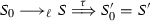   ((5), (3), Lemma 14, with $S = S_0$, $S_1 = S$, $S_2 = \llbracket Q_0 \rrbracket$).

        • (7) $Q_0 \longrightarrow ^{*} Q_0 = Q$    (Fig. 1).

        • (8) $S' \cong ^{\pi }_\ell \llbracket Q \rrbracket$ ((6), (7), (4)).

      • $\diamond ~y(z).Q_2 = \mathbf {*}\, y(z).Q_2$: Similar as above.

    • 3. $\mathsf {sel} (x,l)\in \mathcal {I}_{S_0} \setminus \mathcal {I}_{S}$: As above.

    • 4. $\mathsf {bra} (x,l)\in \mathcal {I}_{S_0} \setminus \mathcal {I}_{S}$: As above.

$\square$

Besides the criteria considered in our definition of valid encoding (Definition 20), Gorla [26] advocates for divergence reflection, a correctness criterion that we informally discuss here, as it is related to operational correspondence. Divergence reflection ensures that every infinite sequence of reductions in a target term corresponds to some infinite sequence of reductions in its associated source term. Let us write $S \xrightarrow {\,~\,}_s^{\omega }$ (resp. $T \xrightarrow {\,~\,}_t^{\omega }$) whenever the source term S (resp. target term T) has such an infinite sequence of reductions. A translation $\llbracket \cdot \rrbracket : \mathcal {L}_s\rightarrow \mathcal {L}_t$ then reflects divergence if for every S such that $\llbracket S \rrbracket \xrightarrow {\,~\,}_t^{\omega }$ then $S \xrightarrow {\,~\,}_s^{\omega }$.

Our translation $\llbracket \cdot \rrbracket {}$ (Fig. 8) reflects divergence. The only sources of infinite behavior it induces concern the translation of restriction, which includes the persistent tell process ${{\,\mathrm{!}\,}}\overline{\{x{:}y\}}$, and the translation of input-guarded replication in $\pi$. The persistent tell cannot reduce by itself; by providing copies of constraint $\{x{:}y\}$, it partakes in target reductions (inferred using Rule ${\lfloor \textsc {C:Sync}\rfloor }$). Importantly, such reductions occur only when an auxiliary predicate (such as $\mathsf {rcv} (x,y)$, added by the translation of a source process) is also in the store. The translation of input-guarded replication does not reduce on its own either: associated reductions depend on synchronizations with (the translation of) corresponding outputs. Therefore, as $\llbracket \cdot \rrbracket {}$ does not induce other forms of infinite behavior, every infinite sequence of reductions emanating from $\llbracket P \rrbracket {}$ corresponds exclusively to infinite reductions present in P.

4.4 Success sensitiveness

Here, we consider success sensitiveness, the last criterion in our definition of valid encoding (Definition 20). For the purpose of proving that our translation satisfies this criterion, we adopt some extensions, following [25, 26]. First, we extend the syntax of $\pi$ (cf. Definition 1) and $\texttt {lcc}$ (Definition 11) with a success process, denoted $\checkmark$ in both languages. In $\pi$, the operational semantics is kept unchanged, assuming that $\checkmark$ is preserved by reduction. That is, if $P \mathord {\,\big |\,}\checkmark$ and $P \longrightarrow ^{*} Q$, then $Q = Q' \mathord {\,\big |\,}\checkmark$, for some $Q'$. The new process $\checkmark$ is assumed to be well-typed. In $\texttt {lcc}$, we define $\checkmark {\mathop {=}\limits ^{\texttt {def} }} {!}\overline{\textit{check}}$, where $\textit{check}$ denotes a constraint that is fresh, i.e., it does not occur anywhere else. Thus, in $\texttt {lcc}$, the success process $\checkmark$ defines $\textit{check}$ as a persistent constraint; in particular, notice that $\llbracket \cdot \rrbracket$ does not introduce abstractions that consume $\textit{check}$.

With process $\checkmark$ in place, we define success predicates for $\pi$ and $\texttt {lcc}$ as the potential that a process has of reducing to a process with a top-level unguarded occurrence of $\checkmark$:

The equivalences in each language (cf. Definition 24) are sensitive to success. That is, it is never the case that $P \equiv _{\pi } Q$ if $P \!\Downarrow _\pi$ but (cf. Definition 2). Similarly, by adding the (fresh) constraint $\textit{check}$ to the set of output observables used as parameter to $\cong ^{\pi }_\ell$ (Definition 22), it is never the case that $P \cong ^{\pi }_\ell Q$ if $P \!\Downarrow _\texttt {lcc}$ but $Q \not \!\Downarrow _\texttt {lcc}$ (cf. Definition 23).

Under these assumptions, success sensitiveness is a property of the translation $\llbracket \cdot \rrbracket$ in Fig. 8, trivially extended with the case $\llbracket \checkmark \rrbracket = {!}\overline{\textit{check}}$. For this (extended) translation, the proof of success sensitiveness, given next, relies on operational completeness and soundness (Theorems 11 and 12), which we assume extended to the source and target languages with success processes.

Theorem 17

(Success Sensitiveness for $\llbracket \cdot \rrbracket$) Let $\llbracket \cdot \rrbracket$ be the translation in Definition 25. Also, let P be a well-typed $\pi$ program. Then, $P \!\Downarrow _\pi$ if and only if $\llbracket P \rrbracket \!\Downarrow _\texttt {lcc}$.

Proof

We consider both directions. Recall that Fig. 8 defines $\llbracket P \mathord {\,\big |\,}Q \rrbracket = \llbracket P \rrbracket \parallel \llbracket Q \rrbracket$.

• 1. If $P \!\Downarrow _\pi$, then $P \longrightarrow ^{*} P'$ and $P' \equiv _{\pi } P '' \mathord {\,\big |\,}\checkmark$. By operational completeness (Theorem 11), there exists an S such that . Because $\cong ^{\pi }_\ell$ is sensitive to success, we have $S \!\Downarrow _\texttt {lcc}$. Therefore, $\llbracket P \rrbracket \!\Downarrow _\texttt {lcc}$.

• 2. If $\llbracket P \rrbracket \!\Downarrow _\texttt {lcc}$, then and $S \equiv S_1 \parallel {!}\overline{\textit{check}}$. By operational soundness (Theorem 12), there exist $Q, S'$ such that $P \longrightarrow ^* Q$ and . Now, because process ${!}\overline{\textit{check}}$ is persistent, we have that $S' = S'' \parallel {!}\overline{\textit{check}}$. Because success is captured by $\cong ^{\pi }_\ell$, we infer that $\llbracket Q \rrbracket = \llbracket Q' \rrbracket \parallel {!}\overline{\textit{check}} = \llbracket Q' \rrbracket \mathord {\,\big |\,}\checkmark$, for some $Q'$. Therefore, $P \longrightarrow ^* Q' \mathord {\,\big |\,}\checkmark$ and we conclude that $P \!\Downarrow _\pi$.

$\square$

We have proven that the translation $\llbracket \cdot \rrbracket$ is name invariant (Theorem 8), compositional (Theorem 9), operationally complete (Theorem 11), operationally sound (Theorem 12), and also success sensitive (Theorem 17). Therefore, we may now state that $\llbracket \cdot \rrbracket$ is a valid encoding:

Corollary 5

The translation $\langle \llbracket \cdot \rrbracket , \varphi _{\llbracket \cdot \rrbracket } \rangle$ (cf. Definition 25) is a valid encoding (cf. Definition 20).

As an application of our encoding and its correctness properties, in the following section we devise a methodology to use encoded terms as macros in $\texttt {lcc}$ contexts; we show how it can be used to enhance $\pi$ specifications with time constraints.

5 The encoding at work

The correctness properties of $\llbracket \cdot \rrbracket$ (in particular, compositionality and operational correspondence) can be used to enhance operational specifications written in $\pi$ with declarative features that can be expressed in $\texttt {lcc}$. We focus on expressing two of the patterns presented by Neykova et al. in [36], where a series of realistic communication protocols with time were analyzed using the Scribble specification language [46].

Next, we overview our approach. Then, in Sects. 5.2 and 5.3 we develop two of the patterns presented in [36] and show how our encoding can help in specifying them in $\texttt {lcc}$.

5.1 Overview: exploiting compositionality via decompositions

As shown before, $\llbracket \cdot \rrbracket$ satisfies correctness properties that ensure that source specifications in $\pi$ can be represented in $\texttt {lcc}$ and that their behavior is preserved (cf. Corollary 5). We are interested in using $\llbracket \cdot \rrbracket$ to represent requirements that may appear in message-passing components but are not explicitly representable in $\pi$. An example of such requirements is: “an acknowledgment message $\texttt {ACK}$ should be sent (by the server) no later than three time units after receiving the request message $\texttt {REQ}$”. As already mentioned, this kind of behavior is not straightforwardly representable in $\pi$. In fact, using $\pi$ we could only represent the interaction in the previous requirement as a request–acknowledgment handshake. Consider the process

$$\begin{aligned} P_h = (\varvec{\nu }xy)({x}\langle \texttt {REQ}\rangle .x(z). \mathbf {0} \mathord {\,\big |\,}y(z'). {y}\langle \texttt {ACK}\rangle . \mathbf {0} ) \end{aligned}$$

(6)

where x represents the endpoint used by the client, while y represents the endpoint of the server. The client sends $\texttt {REQ}$ and then awaits for $\texttt {ACK}$, which is sent by the server.

To represent this kind of requirements, the key idea is to consider encoded terms as macros to be used inside a larger $\texttt {lcc}$ specification. Then, because of the correctness properties we have established for $\llbracket \cdot \rrbracket$, these snippets represent $\texttt {lcc}$ processes that will execute correct communication behavior. For example, using $\llbracket P_h \rrbracket$ we could specify the $\texttt {lcc}$ process

$$\begin{aligned} Q = \mathbf {\forall }{\epsilon }\big (\textit{month}(m) = \textit{january} \rightarrow \llbracket P_h \rrbracket \big ) \end{aligned}$$

which checks that the current month (stored in variable m) is $\textit{january}$; only when this constraint is true, the behavior in $\llbracket P_h \rrbracket$ is executed. Our encoding’s operational correspondence property ensures that the behavior of Q corresponds to that of $P_h$, provided that the guard is satisfied (cf. Theorems 11 and 12). This is useful to represent communication behavior that depends on information that is contextual, i.e., external to the program.

In a way, Q defines a constraint over the whole process $P_h$. It can be desirable to constrain only some of the actions of $P_h$. For the sake of illustration, let us imagine a variant of $\pi$ in which prefixes are annotated:

$$\begin{aligned} P'_h = (\varvec{\nu }xy)({x}\langle \texttt {REQ}\rangle .x^{3}(z). \mathbf {0} \mathord {\,\big |\,}y(z'). {y}\langle \texttt {ACK}\rangle . \mathbf {0} ) \end{aligned}$$

(7)

Above, prefix $x^{3}(z). \mathbf {0}$ says that the input action should take place within three time units after the preceding action. This defines a timed requirement connecting two separate actions.

To specify processes such as $P'_h$ using our encoding, we consider $\pi$ processes that have been decomposed in such a way that every prefix appears in an independent parallel process. Such a decomposition should preserve the order in which actions are executed (as dictated by session types). In this way, the compositionality property of our encoding gives us control over specific parts of the translated $\pi$ process, allowing us to define constraints on the translations of some specific prefixes (cf. Theorem 10).

Decompositions of (un)typed $\pi$-calculus processes have been studied as trios processes and minimal session types [1, 38]. The idea in [38] is to transform a process P into an equivalent process formed only by trios, sequential processes with at most three prefixes. Each trio emulates a specific prefix of P; trios interact in such a way that every sub-term is executed at the right time, to ensure that the causal order of interactions in P is preserved. Building upon this idea, the work of Arslanagic et al. on minimal session types [1] considers decompositions of processes and of their associated session types.

We shall build upon the decomposition strategy in [1, 38] and leave an in-depth study of decompositions for $\pi$ for follow up work. We generate $\pi$ processes in which each prefix is represented by a parallel sub-process, while preserving the causal order of the given process. Then, using the compositionality of $\llbracket \cdot \rrbracket$ (Theorem 9), we obtain an appropriate granularity level for the analysis of code snippets (obtained from trios) in $\texttt {lcc}$ specifications.

For the sake of illustration, we follow [1] and consider the decomposition of well-typed programs from the finite fragment of $\pi$ without selection and branching (i.e., output, input, restriction, parallel composition, and inaction). Since decompositions based on trios processes require polyadic communication, we shall assume the following shorthand notations:

$$\begin{aligned} \begin{aligned}&{x}\langle \widetilde{v}\rangle .P = {x}\langle v_1\rangle .\ldots .{x}\langle v_n\rangle .P \quad (|\widetilde{v}| = n \wedge n\ge 1) \\&x(\widetilde{y}).P = x(y_1).\ldots .x(y_n).P \quad (|\widetilde{y}| = n \wedge n\ge 1) \end{aligned} \end{aligned}$$

We use $\textit{size}(\cdot )$ and $\mathsf {size}(\cdot )$ to denote the size of process P and type T, respectively (cf. Fig. 15). With these auxiliary functions, we define the following decomposition function:

Fig. 15

Size of a process (resp. type) in the finite fragment of $\pi$

Definition 36

(Decomposition) Let $P= (\varvec{\nu }x_1y_1)\ldots (\varvec{\nu }x_ny_n)Q$ be a well-typed program in the finite fragment of $\pi$ and $\varGamma = \{x_1 : T_1, y_1:\overline{T_1}, \ldots , x_n: T_n, y_n:\overline{T_n}\}$ be a context such that $\varGamma \vdash Q$. The decomposition of P, denoted $\mathfrak {D}(P)$, is defined as

where:

• (1) $\widetilde{u} = \widetilde{x_1}\widetilde{y_1}\ldots \widetilde{x_n}\widetilde{y_n}$, $\widetilde{w} = x_1y_1\ldots x_ny_n$, and $\widetilde{w'} = x_{1,1}y_{1,1}\ldots x_{n,1}y_{n,1}$.

• (2) $\widetilde{x_i} = x_{i,1}\ldots x_{i,m}$ and $\widetilde{y_i} = y_{i,1}\ldots y_{i,m}$ with $m = \mathsf {size}(T_i)$ for every $i\in \{1,\ldots ,m\}$.

• (3) $\widetilde{c} = c_1\ldots c_r$ and $\widetilde{d} = d_1 \ldots d_r$ with $r = \textit{size}(P)$.

• (4) $\mathfrak {B}^{k}_{\widetilde{u}}(P)$ is defined inductively over the finite fragment of $\pi$ as in Fig. 16.

Fig. 16

Breakdown function for the processes in the finite fragment of $\pi$

Remark 3

We decompose only well-typed programs (cf. Notation 3). Theorem 4 ensures that for every program P to be decomposed, it holds that $P = (\varvec{\nu }x_1y_1)\ldots (\varvec{\nu }x_ny_n)Q$, with $n\ge 0$. (For simplicity, we shall also assume no $(\varvec{\nu }x'y')$ occurs in Q.) Moreover, typability ensures there exists a context $\varGamma = \{x_1 : T_1, y_1:\overline{T_1}, \ldots , x_n: T_n, y_n:\overline{T_n}\}$ such that $\varGamma \vdash Q$.

Fig. 17

A process decomposition. We let $\widetilde{u_x} = x_{1,1}x_{1,2}$, $\widetilde{u_y} = y_{1,1}y_{1,2}$, and $\widetilde{u} = \widetilde{u_x},\widetilde{u_y}$

Figure 17 illustrates $\mathfrak {D}(P_h)$, the process decomposition of $P_h$ obtained from Definition 36. We shall use this decomposition to represent the timed behavior required by $P'_h$. Let us first analyze how parallel sub-processes in $\mathfrak {D}(P_h)$ implement individual prefixes of $P_h$:

• process $c_2(\widetilde{u_x}).{x_{1,1}}\langle \texttt {REQ}\rangle .{d_3}\langle x_{1,2}\rangle .\mathbf {0}$ implements prefix ${x}\langle \texttt {REQ}\rangle$.

• process $c_3(x_{1,2}).x_{1,2}(z).{d_4}\langle z\rangle .\mathbf {0}$ implements prefix x(z).

• process $c_4(w).\mathbf {0}$ implements $\mathbf {0}$.

The sub-processes of $\mathfrak {D}(P_h)$ that do not correspond to a prefix in $P_h$ are auxiliary processes that trigger the prefix representations. Process $\mathfrak {D}(P_h)$ is typable under the appropriate contexts. This is because, by definition, there are no shared variables and each pair of covariables implement complementary behaviors. Also, the decomposition can be shown to preserve the causal order of the source process [1, 38]. In our example, the order implemented by $P_h$ to send messages $\texttt {REQ}$ and $\texttt {ACK}$ is preserved by $\mathfrak {D}(P_h)$—see App. A for the associated reduction steps. We may then argue that $P_h$ and $\mathfrak {D}(P_h)$ execute the same protocol, up to the synchronizations added by the decomposition.

By using $\mathfrak {D}(P_h)$ instead of $P_h$ as the source process for $\llbracket \cdot \rrbracket$, we can modularly treat translations for each prefix of $P_h$ (i.e., its trios) as “black boxes” in $\texttt {lcc}$. Our operational correspondence results (Theorems 11 and 12) ensure that these black boxes correctly mimick the behavior of $\mathfrak {D}(P_h)$. This allows us to safely “plug” these black boxes into a larger $\texttt {lcc}$ specification with additional declarative requirements, thus going beyond the merely operational specification given by $P_h$. For example, we can define an $\texttt {lcc}$ process that specifies the timed conditions in $P'_h$ in (7), which cannot be implemented easily in $\pi$.

We now use these ideas to develop $\texttt {lcc}$ specifications of two of the communication patterns presented in [36]—they are graphically represented in Fig. 18(a) and (b). These patterns will allow us to use $\texttt {lcc}$ to specify processes such as $P'_h$.

5.2 Request–response timeout

This pattern is used to enforce requirements on the timing of a response, ensuring quality of service; it can be required both at server or client side (cf. Fig. 18a). Process $P'_h$ can be seen as a specific implementation of this pattern. In [36] three use cases are identified:

Fig. 18

Timed patterns for communicating systems

• (1) In [19], a service is requested to respond timely: “an acknowledgment message $\texttt {ACK}$ should be sent (by the server) no later than one second after receiving the request message $\texttt {REQ}$”.

• (2) Similarly, also in [19], a Travel Agency web service specifies the pattern at the client side: “A user should be given a response $\texttt {RES}$ within one minute of a given request $\texttt {REQ}$”.

• (3) Finally, extracted from the Simple Mail Transport Protocol specification [30], we have a requirement that exhibits a composition of request–response timeout patterns: “a user should have a five minutes timeout for the $\texttt {MAIL}$ command and a three minutes timeout for the $\texttt {DATABLOCK}$ command”.

Requirement (1) above (i.e., the pattern at the server side) specifies that a reply should be sent within a fixed amount of time after the request have been received. In Requirement (2), which represents the client side, the server must be ready to receive the client’s response within a fixed amount of time. In general, these patterns can be written as:

• (a) Server side: After receiving a message $\texttt {REQ}$ from $\texttt {A}$, $\texttt {B}$ must send the acknowledgment $\texttt {ACK}$ within $t_{\texttt {A}}$ time units.

• (b) Client side: After sending a message $\texttt {REQ}$ to $\texttt {B}$, $\texttt {A}$ must be able to receive the acknowledgment $\texttt {ACK}$ from $\texttt {B}$ within $t_{\texttt {B}}$ time units.

A possible $\pi$ specification for this pattern is shown below. We use a more general version of $P'_h$ in (7), which is informally annotated to describe the intended timing requirements:

$$\begin{aligned} \begin{aligned} P_r = (\varvec{\nu }xy)(\underbrace{{x}\langle \texttt {REQ}\rangle .x(z).Q_1 \mathord {\,\big |\,}y(z). {y}\langle \texttt {ACK}\rangle }_{t}.Q_2) \end{aligned} \end{aligned}$$

(8)

The intent is that the time elapsed between the reception of the request and the acknowledgment must not exceed t time units.

We now present a decomposition for $P_r$, following Definition 36:

$$\begin{aligned} \begin{aligned} \mathfrak {D}(P_r) = (\varvec{\nu }\widetilde{u})(\mathfrak {D}_1 \mathord {\,\big |\,}\mathfrak {D}_2 \mathord {\,\big |\,}\mathfrak {D}_4 \mathord {\,\big |\,}\mathfrak {D}_3 \mathord {\,\big |\,}R ) \end{aligned} \end{aligned}$$

(9)

where we assume that R contains the decompositions for processes $Q_1$ and $Q_2$ (not needed in this example), that $\widetilde{u}$ can be obtained from Definition 36, and that each of the parallel sub-processes $\mathfrak {D}_i$ ($i\in \{1,2,3,4\}$) represents a prefix in $P_r$:

$$\begin{aligned} \begin{aligned} \mathfrak {D}_1&= c_2(\widetilde{u_x}).{x_{1,1}}\langle \texttt {REQ}\rangle .{d_3}\langle \widetilde{u_x}\setminus x_{1,1} \rangle .\mathbf {0} \\ \mathfrak {D}_2&= c_3(\widetilde{u_x}\setminus x_{1,1}).x_{1,2}(z\widetilde{z_1}).{d_4}\langle \widetilde{u_x}z\widetilde{z_1}\setminus x_{1,1}x_{1,2}\rangle .\mathbf {0} \\ \mathfrak {D}_3&= c_5(\widetilde{u_y}).y_{1,1}(z'\widetilde{z_2}).{d_6}\langle \widetilde{u_y}z'\widetilde{z_2}\setminus y_{1,1}\rangle .\mathbf {0} \\ \mathfrak {D}_4&= c_6(\widetilde{u_y}z'\widetilde{z_2}\setminus y_{1,1}).{y_{1,2}}\langle \texttt {ACK}\rangle .{d_7}\langle \widetilde{u_y}z'\widetilde{z_2}\setminus y_{1,1}y_{1,2}\rangle .\mathbf {0} \end{aligned} \end{aligned}$$

By applying $\llbracket \cdot \rrbracket$ and thanks to Theorem 9, we can use the translations of each $\mathfrak {D}_i$ ($i\in \{1,2,3,4\}$) as part of an $\texttt {lcc}$ process that represents the request–response timeout pattern:

$$\begin{aligned} S_1 = C_{\widetilde{u}}[ \llbracket \mathfrak {D}_1 \rrbracket \parallel \mathbf {\forall }{\epsilon }(clock(x)\le t \rightarrow \llbracket \mathfrak {D}_2 \rrbracket ) \parallel \llbracket \mathfrak {D}_3 \rrbracket \parallel \llbracket \mathfrak {D}_4 \rrbracket \parallel \llbracket R \rrbracket ] \end{aligned}$$

where $\widetilde{u}$ can be obtained by following Definition 36. We can also exploit non-deterministic choices in $\texttt {lcc}$ to signal that the process fails after a time-out:

$$\begin{aligned} \begin{aligned} S_2 = \exists \widetilde{x}\widetilde{y}. \big (&\llbracket \mathfrak {D}_1 \rrbracket \parallel (\mathbf {\forall }{\epsilon }(clock(u)\le t \rightarrow \llbracket \mathfrak {D}_2 \rrbracket ) + \mathbf {\forall }{\epsilon }(clock(u)> t \rightarrow Q_f)) \parallel \\ {}&\llbracket \mathfrak {D}_3 \rrbracket \parallel \llbracket \mathfrak {D}_4 \rrbracket \parallel \llbracket R \rrbracket \big ) \end{aligned} \end{aligned}$$

Whenever $clock(u)>t$, process $S_2$ reduces to process $Q_f$ which represents the actions that must be taken in case the timing constraint is not met. Interestingly, if $Q_f$ is taken to represent an error process, then the behavior would be reminiscent of the input operators with deadlines presented in [9], which evolve into a failure whenever a deadline is not met.

The operational correspondence property of $\llbracket \cdot \rrbracket$ (cf. Theorems 11 and 12) ensures that $S_2$ preserves the behavior of the source $\pi$ processes, whenever the timing constraint is met.

5.3 Messages in a time-frame

This pattern enforces a limit on the number of messages exchanged within a given time-frame (cf. Fig. 18b). In [36] two use cases from [19] were identified:

• (1) Controlling denial of service attacks: “a user is allowed to send only three redirect messages to a server with an interval between the messages of no less than two time units”.

• (2) Used in a Travel Agency web service: “a customer can change the date of his travel only two times and this must happen between one and five days of the initial reservation”.

This pattern concerns message repetition, which can be specified in two ways. We can (a) require the repetition to occur at a specified pace; i.e., requiring that messages can only be sent in intervals of time, or (b) specify an overall time-frame for the messages to be sent.

We generalize these patterns next. Keeping consistency with Fig. 18b, we will use t for the interval pattern and $t'$, for the overall time-frame pattern. We use r and $r'$ to denote the upper bound of the time-frames, i.e., $t\le i \le r$ (resp. $t'\le i \le r'$), where i stands for the “safe time” for sending messages.

• (a) Interval: $\texttt {A}$ is allowed to send $\texttt {B}$ at most k messages, and at time intervals of at least t and at most r time units.

• (b) Overall time-frame: $\texttt {A}$ is allowed to send $\texttt {B}$ at most k messages in the overall time-frame of at least $t'$ and at most $r'$ time units.

To represent these two variants of the pattern using $\llbracket \cdot \rrbracket$, we first present two $\pi$ processes, annotated to indicate the timing constraints:

$$\begin{aligned} P_{ti}&= (\varvec{\nu }xy)(x\langle \underbrace{\texttt {M}_1\rangle .x\langle }_{t_1}\underbrace{\texttt {M}_2\rangle .x\langle }_{t_1}\underbrace{\texttt {M}_3\rangle .x\langle }_{t_1}\texttt {M}_4\rangle .P_x \mathord {\,\big |\,}P_y) \\ P_{to}&= (\varvec{\nu }xy)(\underbrace{{x}\langle \texttt {M}_1\rangle .{x}\langle \texttt {M}_2\rangle .{x}\langle \texttt {M}_3\rangle .{x}\langle \texttt {M}_4\rangle }_{t_2}.P_x \mathord {\,\big |\,}P_y) \end{aligned}$$

Processes $P_{ti}$ and $P_{to}$ differ only on their timing constraints (i.e., the annotations below). They both send four messages that must be received by some $P_y$ (which we leave unspecified). Process $P_{ti}$ represents the interval pattern, in which we must leave at least $t_1$ time units between each message. Process $P_{to}$ represents the overall time-frame pattern in which all the four messages must be sent in an overall time of $t_2$ time units. Here, we use $\textit{clock}(u_1)$ and $\textit{clock}(u_2)$ to represent the time elapsed in clocks $u_1$ and $u_2$, respectively.

We start by considering the decompositions of $\mathfrak {D}(P_{ti})$ and $\mathfrak {D}(P_{to})$:

$$\begin{aligned} \begin{aligned} \mathfrak {D}(P_{to}) = \mathfrak {D}(P_{ti}) = (\varvec{\nu }\widetilde{u})(\mathfrak {D}_1 \mathord {\,\big |\,}\mathfrak {D}_2 \mathord {\,\big |\,}\mathfrak {D}_3 \mathord {\,\big |\,}\mathfrak {D}_4 \mathord {\,\big |\,}R_x \mathord {\,\big |\,}R_y) \end{aligned} \end{aligned}$$

(10)

where we assume that $R_x$ and $R_y$ contain the decompositions of $P_x$ and $P_y$, respectively. The sequence $\widetilde{u}$ can be derived from Definition 36. Processes $\mathfrak {D}_i$ ($i\in \{1,2,3,4\}$) correspond to:

$$\begin{aligned} \begin{aligned} \mathfrak {D}_1&= c_2(\widetilde{u_x}).{x_{1,1}}\langle \texttt {M}_1\rangle .{d_3}\langle \widetilde{u_x}\setminus x_{1,1}\rangle .\mathbf {0} \\ \mathfrak {D}_2&= c_3(\widetilde{u_x}\setminus x_{1,1}).{x_{1,2}}\langle \texttt {M}_2\rangle .{d_4}\langle \widetilde{u_x}\setminus x_{1,1}x_{1,2}\rangle .\mathbf {0} \\ \mathfrak {D}_3&= c_4(\widetilde{u_x}\setminus x_{1,1}x_{1,2}).{x_{1,3}}\langle \texttt {M}_3\rangle .{d_5}\langle \widetilde{u_x}\setminus x_{1,1}x_{1,2}x_{1,3}\rangle .\mathbf {0} \\ \mathfrak {D}_4&= c_5(\widetilde{u_x}\setminus x_{1,1}x_{1,2}x_{1,3}).{x_{1,4}}\langle \texttt {M}_4\rangle .{d_6}\langle \widetilde{u_x}\setminus x_{1,1}x_{1,2}x_{1,3}x_{1,4}\rangle .\mathbf {0} \\ \end{aligned} \end{aligned}$$

By applying $\llbracket \cdot \rrbracket$, and thanks to Theorems 9 and 10, we have:

$$\begin{aligned} \llbracket \mathfrak {D}(P_{ti}) \rrbracket = \llbracket \mathfrak {D}(P_{to}) \rrbracket = C_{\widetilde{x}\widetilde{y}}[ \llbracket \mathfrak {D}_1 \rrbracket \parallel \llbracket \mathfrak {D}_2 \rrbracket \parallel \llbracket \mathfrak {D}_3 \rrbracket \parallel \llbracket \mathfrak {D}_4 \rrbracket \parallel \llbracket R_x \rrbracket \parallel \llbracket R_y \rrbracket ] \end{aligned}$$

We now represent the variants of the timed pattern above (i.e., (a) and (b)) using $\llbracket \cdot \rrbracket$:

• (1) Interval: This variant requires that for every sent message, the next message is sent with a delay of at least $t_1$ time units. This means guarding the snippets obtained with the decomposition so that the processes are suspended until the interval $t_1$ has passed:

  $$\begin{aligned} \begin{aligned} Q_1 = C_{\widetilde{x}\widetilde{y}}[&\llbracket \mathfrak {D}_1 \rrbracket \parallel \mathbf {\forall }{\epsilon }\big (clock(u_1)> t_1 \rightarrow \llbracket \mathfrak {D}_2 \rrbracket \parallel \overline{rst(u_1)} \parallel \\&\mathbf {\forall }{\epsilon }\big (clock(u_1)> t_1 \rightarrow \llbracket \mathfrak {D}_3 \rrbracket \parallel \overline{rst(u_1)} \parallel \\&\mathbf {\forall }{\epsilon }\big (clock(u_1)> t_1 \rightarrow \llbracket \mathfrak {D}_4 \rrbracket \parallel \overline{rst(u_1)}\big ) \big ) \parallel \\&\mathbf {\forall }{\epsilon }\big (clock(u_1) > t_1 \rightarrow \llbracket R_x \rrbracket \big ) \big ) \parallel \llbracket R_y \rrbracket ] \end{aligned} \end{aligned}$$

  Above, constraint $rst(u_1)$ tells the store that clock $u_1$ must be reset. Process $Q_1$ consists of nested abstractions. Each abstraction is used to make the next synchronization wait until the delay is satisfied. To achieve this, we guard each abstraction with constraint $clock(u_1) > t_1$. In this way, we ensure that the process representing each prefix is delayed accordingly. We also ensure that whenever the timing constraint is met, the clock is reset to allow for the time to count from the start once again.

• (2) Overall Time-Frame: This variant can be represented by changing the timing constraint in $Q_1$ to $\textit{clock}(u_2)\le t_2$ and by not resetting the clock inside every abstraction:

  $$\begin{aligned} \begin{aligned} Q_2 = C_{\widetilde{x}\widetilde{y}}[&\mathbf {\forall }{\epsilon }\big (clock(u_2) \le t_2 \rightarrow \llbracket \mathfrak {D}_1 \rrbracket \parallel \mathbf {\forall }{\epsilon }\big (clock(u_2) \le t_2 \rightarrow \llbracket \mathfrak {D}_2 \rrbracket \parallel \\&\mathbf {\forall }{\epsilon }\big (clock(u_2) \le t_2 \rightarrow \llbracket \mathfrak {D}_3 \rrbracket \parallel \mathbf {\forall }{\epsilon }\big (clock(u_2) \le t_2 \rightarrow \llbracket \mathfrak {D}_4 \rrbracket \parallel \overline{rst(u_2)}\big ) \big ) \parallel \\&\mathbf {\forall }{\epsilon }\big (clock(u_2)\le t_2 \rightarrow \llbracket R_x \rrbracket \big ) \big ) \big ) \parallel \llbracket R_y \rrbracket ] \end{aligned} \end{aligned}$$

  The overall time of the communications can be checked because we only reset the clock at the end of the complete interaction.

Both $Q_1$ and $Q_2$ preserve the behavior of their source process, assuming that all timing constraints are satisfied. This is because of the operational correspondence property (cf. Theorems 11 and 12). Similarly to the $\texttt {lcc}$ specification of the request–response timeout, we can use non-determinism in $\texttt {lcc}$ to extend the behavior of the declarative implementations.

6 Related work

The most related work is [31], already discussed, which uses $\texttt {utcc}$ as target language in a translation of a session $\pi$-calculus different from $\pi$. By using $\texttt {lcc}$ rather than $\texttt {utcc}$, we can correctly encode processes that cannot be represented in [31] (cf. Ex. 3). Also, linearity in $\texttt {lcc}$ allows us to provide operational correspondence results (cf. Theorems 11 and 12) stronger than those in [31].

Haemmerlé [27] develops an encoding of an asynchronous $\pi$-calculus into $\texttt {lcc}$, and establishes operational correspondence for it. Since his encoding concerns two asynchronous models, this operational correspondence is more direct than in our case. Monjaraz and Mariño [35] encode the asynchronous $\pi$-calculus into Flat Guarded Horn Clauses. They consider compositionality and operational correspondence criteria, as we do here. In contrast to [27, 35], here we consider a session $\pi$-calculus with synchronous communication, which adds challenges in the translation and its associated correctness proofs. The developments in [27, 35] are not concerned with the analysis of message-passing programs in general, nor with session-based concurrency in particular.

Loosely related to our work are [8, 18]. Bocchi et al. [8] integrate declarative requirements into multiparty session types by enriching (type-based) protocol descriptions with logical assertions which are globally specified within multiparty protocols and potentially projected onto specifications for local participants. Rather than a declarative process model based on constraints, the target process language in [8] is a $\pi$-calculus with predicates for checking (outgoing and incoming) communications. It should be interesting to see if such an extended session $\pi$-calculus can be encoded into $\texttt {lcc}$ by adapting our encoding. Also in the context of choreographies, although in a different vein, Carbone et al. [18] explore declarative reasoning via a variant of Hennessy–Milner logic for global specifications.

Prior works on Web service contracts have integrated operational descriptions (akin to CCS specifications) and constraints, where constraint entailment represents the possibility for a service to comply with the requirements of a requester. Buscemi and Montanari’s CC-pi [12, 14] combines the message-passing communication model from the $\pi$-calculus with operations over a store as in $\texttt {ccp}$ languages. Analysis techniques for CC-pi processes exploit behavioral equivalences [13]; logical characterizations of process behavior have not been studied. A challenge for obtaining such characterizations is CC-pi’s retract construct, which breaks the monotonicity requirements imposed for stores in the $\texttt {ccp}$ model. We do not know of any attempts on applying session-type analysis for specifications in CC-pi.

Coppo and Dezani-Ciancaglini [20] extend the session $\pi$-calculus in [29] with constraint handling operators, such as tells, asks and constraint checks. Session initiation is then bound to the satisfaction of constraint in the store. The merge of constraints and a session-type system guarantees bilinearity, i.e., channels in use remain private, and that the communications proceed according to the prescribed session types. It is worth noticing that the underlying store in [20] is not linear, which can create potential races among different service providers.

The interplay of constraints and contracts has been also studied by Buscemi et al. [10]. In their model, service interactions follow three phases: negotiation, commitment, and execution. In the negotiation phase, processes agree in fulfilling certain desired behaviors, without guarantee of success. Once committed, it is guaranteed that process execution will honor promised behaviors. The model in [10] uses two languages: a variant of CCS is used as a source language, where the behavior of services and clients is specified; these specifications are then compiled to a language based on CC-pi with no retraction operator, where constraints ensure that interactions between clients and services do not deadlock. It would be insightful to enrich this two-level model by using linear constraints as in $\texttt {lcc}$, so as to refine the consumption of resources in the environment.

Bartoletti et al. [2, 4] promote contract-oriented computing as a novel vision for enforcing service behaviors at runtime. The premise is that in scenarios where third-party components can be used but not inspected, verification based on (session) types becomes a challenge. Contracts exhibit promises about the expected runtime behavior of each component; they can be used to establish new sessions (contract negotiation) and to enforce that components abide to their promised behavior (honesty). The calculus for contracting processes is based on PCL, a propositional contract logic with a contractual form of implication [4]; this enables to express multiparty assume-guarantee specifications where services only engage in a communication once there are enough guarantees that their requirements will be fulfilled. PCL is used as the underlying constraint system for the contract language used in [4], a variant of $\texttt {ccp}$ with name-passing primitives. In [3], the expressive power of the contract calculus is analyzed with respect to the synchronous $\pi$-calculus; name-invariance, compositionality, and operational correspondence are established, as we do here. In [2] the authors introduce $CO_2$, a generic framework for contract-oriented computing. A characterization of contracts as processes and as formulas in PCL has been developed.

More applications of the encoding herein presented can be found in Cano’s PhD thesis [15]. They include an extension of $\pi$ with session establishment, which is encoded into an extension of $\texttt {lcc}$ with private information, following [28]. Moreover, the thesis [15] also includes an extended account of the work in [16], in which different variants of the session $\pi$-calculus in [45] are encoded into the reactive language ReactiveML  [32].

7 Concluding remarks

We have presented an encoding of the session $\pi$-calculus $\pi$ into $\texttt {lcc}$, a process language based on the $\texttt {ccp}$ model. Our encoding is insightful because $\texttt {lcc}$ and $\pi$ are very different: $\texttt {lcc}$ is declarative, whereas $\pi$ is operational; communication in $\texttt {lcc}$ is asynchronous, based on a shared memory, whereas communication in $\pi$ is point-to-point, based on message passing. Our encoding reconciles these differences and explains precisely how to simulate the operational behavior of $\pi$ using declarative features in $\texttt {lcc}$. In a nutshell, our encoding “decouples” point-to-point communication in $\pi$ by exploiting synchronization on two constraints. Remarkably, because $\texttt {lcc}$ treats constraints as linear, consumable resources we can correctly represent well-typed $\pi$ processes that should feature linear behavior—communication actions governed by session types must occur exactly once. Thus, linearity sharply arises as the common trait in our expressiveness results.

The strong correctness properties that we establish for our encoding demonstrate that $\texttt {lcc}$ can provide a unified account of operational and declarative requirements in message-passing programs. We have followed the encodability criteria by Gorla [26], namely name invariance, compositionality, operational correspondence, and success sensitiveness. In particular, our encoding enjoys the exact same formulation of operational correspondence defined in [26]. These correctness properties guarantee that the behavior of source terms is preserved and reflected appropriately by target terms.

The correctness properties of our encoding hold for $\pi$ processes that are well-typed. Types not only allow us to concentrate on a meaningful class of source processes; they also allow us to address the differences between $\pi$ and $\texttt {lcc}$, already mentioned. In fact, well-typed $\pi$ processes have a syntactic structure that can be precisely characterized and is stable under reductions. Moreover, the compositional nature of our encoding ensures that this structure is retained by translated $\texttt {lcc}$ processes (target terms) and turns out to be essential in analyzing their behavior. In this analysis, we reconstructed the behavior of source processes via the constraints that their corresponding target terms consume or add to the store during reductions. As such, this reconstruction is enabled by observables induced by the semantics of $\texttt {lcc}$. By combining information about the syntactic structure and the observable behavior of target terms, we were able to establish several invariant properties which are in turn central to prove operational correspondence, in particular soundness.

Well-typed session $\pi$-calculi processes can contain rather liberal forms of non-deterministic behavior, which are enabled by the unrestricted types in $\pi$  (cf. [45]). The soundness property for our translation (Theorem 12) holds for a sub-class of the well-typed processes in [45], namely those without output races. We identified this sub-class in a relatively simple way, via a specialization of the predicates that govern typing in [45]. We conjecture that the machinery we have developed for proving soundness can be extended to the whole class of typable processes in [45], provided some additional mechanism that circumvents the value ambiguities mentioned in Sect. 2. We leave this interesting open question for follow-up work.

As application of our results and approach, we have shown how to use our encoding to represent relevant timed patterns in communication protocols, as identified by Neykova et al. [36]. Such timed patterns are commonly found in practice (see, e.g., [19]). Hence, they serve as a valuable validation for our approach. Indeed, thanks to the operational correspondence and compositionality properties, translations of $\pi$ processes can be used as “black boxes” whose behavior correctly mimics the source terms. These boxes can be plugged inside $\texttt {lcc}$ contexts to obtain specifications that exhibit features not easily representable in $\pi$. This way, we can analyze message-passing programs in the presence of partial and contextual information.

Appendices

Additional examples

In this appendix we further develop the examples presented in the main text.

Example 7

(Observables in the translation (cf. Definition 22)) We recall the processes, translations, and observables in Ex. 4:

$$\begin{aligned} P_{3} = (\varvec{\nu }xy)(x \triangleleft {\textit{buy}}.\,{x}\langle 5406\rangle .\,x(inv). \mathbf {0} \mathord {\;|\;}y \triangleright \{{\textit{buy}: } y(w).{y}\langle \mathsf {invoice} \rangle .\mathbf {0} , {\textit{quit}: } y(w'). \mathbf {0} \} ) \end{aligned}$$

(11)

The translation of $P_{3}$ is then given below:

$$\begin{aligned}&\llbracket P_{3} \rrbracket = \exists x,y. \big ({{\,\mathrm{!}\,}}\overline{\{x{:}y\}} \parallel \overline{\mathsf {sel} (x,{\textit{buy}})} \parallel \mathbf {\forall }{u_1}(\mathsf {bra} (u_1,{\textit{buy}})\otimes \{x{:}u_1\} \rightarrow \\&\qquad \qquad \qquad \quad \quad \quad \quad \overline{\mathsf {snd} (x,5406)} \parallel \mathbf {\forall }{u_2}(\mathsf {rcv} (u_2,5406) \otimes \{x{:}u_2\} \rightarrow \llbracket x(inv). \mathbf {0} \rrbracket )) \parallel \\&~\mathbf {\forall }{l,w}(\mathsf {sel} (w,l)\otimes \{w{:}y\} \rightarrow \overline{\mathsf {bra} (y,l)} \parallel \\&\quad \quad \mathbf {\forall }{\epsilon }(l = {\textit{buy}} \rightarrow \mathbf {\forall }{w_1,w}(\mathsf {snd} (w_1,w)\otimes \{w_1{:}y\} \rightarrow \overline{\mathsf {rcv} (y,w)} \parallel \llbracket {y}\langle \mathsf {invoice}\rangle . \mathbf {0} \rrbracket )) \parallel \\&\mathbf {\forall }{\epsilon }(l = {\textit{quit}} \rightarrow \mathbf {\forall }{w_2,u}(\mathsf {snd} (w_2,u)\otimes \{w_2{:}y\} \rightarrow \overline{\mathsf {rcv} (y,u)} \parallel \llbracket y(w'). \mathbf {0} \rrbracket )) ) \big ) \end{aligned}$$

with observables:

$$\begin{aligned}&{\mathcal {O}^{\mathcal {D}^{\star }_{\pi }}(\llbracket P_{3} \rrbracket ) } = \{(\exists x,y. \mathsf {sel} (x,{\textit{buy}})),(\exists x,y. \mathsf {bra} (y,{\textit{buy}})), (\exists x,y. \mathsf {snd} (x,5406)), \\&\,\,(\exists x,y.\mathsf {rcv} (y,5406)), (\exists x,y. \mathsf {snd} (y,\mathsf {invoice})), (\exists x,y. \mathsf {rcv} (x,\mathsf {invoice})), (\exists x,y. \texttt {tt})\} \\&\mathcal {O}^{\mathcal {D}_{\pi }}(\llbracket P_{3} \rrbracket ) = \{(\exists x,y. \mathsf {sel} (x,{\textit{buy}})),(\exists x,y. \mathsf {snd} (x,5406)), (\exists x,y. \mathsf {snd} (y,\mathsf {invoice})) \} \end{aligned}$$

Below, we analyze the single $\tau$-transition for the translation of $P_{3}$ (i.e., $\llbracket P_{3} \rrbracket \longrightarrow _\ell S_1$):

$$\begin{aligned}&S_1=\exists x,y. \big ( {{\,\mathrm{!}\,}}\overline{\{x{:}y\}} \parallel \overline{\mathsf {bra} (y,{\textit{buy}})} \parallel \mathbf {\forall }{u_1}(\mathsf {bra} (u_1,{\textit{buy}})\otimes \{x{:}u_1\} \rightarrow \overline{\mathsf {snd} (x,5406)} \parallel \\&\qquad \qquad \qquad \qquad \mathbf {\forall }{u_2}(\mathsf {rcv} (u_2,5406) \otimes \{x{:}u_2\} \rightarrow \llbracket x(inv). \mathbf {0} \rrbracket )) \parallel \\&\qquad \mathbf {\forall }{\epsilon }({\textit{buy}} = {\textit{buy}} \rightarrow \mathbf {\forall }{w_1,w}(\mathsf {snd} (w_1,w)\otimes \{w_1{:}y\} \rightarrow \overline{\mathsf {rcv} (y,w)} \parallel \llbracket {y}\langle \mathsf {invoice}\rangle . \mathbf {0} \rrbracket )) \parallel \\&\qquad \mathbf {\forall }{\epsilon }({\textit{buy}} = {\textit{quit}} \rightarrow \mathbf {\forall }{w_2,u}(\mathsf {snd} (w_2,u)\otimes \{w_2{:}y\} \rightarrow \overline{\mathsf {rcv} (y,u)} \parallel \llbracket y(w'). \mathbf {0} \rrbracket )) \big ) \end{aligned}$$

Let us now consider the output observables of $S_1$:

$$\begin{aligned} \mathcal {O}^{\mathcal {D}_{\pi }}(S_1) = \{\exists x,y. \mathsf {snd} (x,5406), \exists x,y. \mathsf {snd} (y,\mathsf {invoice})\} \end{aligned}$$

For the sake of comparison, consider the reduction of $P_{3}$, using Rule ${\lfloor \textsc {Sel}\rfloor }$, which discards the second labeled branch:

$$\begin{aligned} P_{3} \longrightarrow (\varvec{\nu }x y)( {x}\langle 5406\rangle . \,x(inv). \mathbf {0} \mathord {\;|\;}y(w). {y}\langle \mathsf {invoice}\rangle . \mathbf {0} ) = P'_{3} \end{aligned}$$

The translation of $P'_{3}$ is as follows (we also show its reduction):

$$\begin{aligned} \llbracket P'_{3} \rrbracket&= \exists x,y. \big ( {{\,\mathrm{!}\,}}\overline{\{x{:}y\}} \parallel \overline{\mathsf {snd} (x,5406)} \parallel \mathbf {\forall }{u_2}(\mathsf {rcv} (u_2,5406)\otimes \{x{:}u_2\} \rightarrow \llbracket x(inv). \mathbf {0} \rrbracket ) \parallel \\&\quad \quad \qquad \quad \mathbf {\forall }{w_1,w}(\mathsf {snd} (w_1,w)\otimes \{w_1{:}y\} \rightarrow \overline{\mathsf {rcv} (y,w)} \parallel \llbracket {y}\langle \mathsf {invoice}\rangle . \mathbf {0} \rrbracket ) \big )\\&\longrightarrow _\ell \exists x,y. \big ( {{\,\mathrm{!}\,}}\overline{\{x{:}y\}} \parallel \mathbf {\forall }{u_2}(\mathsf {rcv} (u_2,5406)\otimes \{x{:}u_2\} \rightarrow \llbracket x(inv). \mathbf {0} \rrbracket ) \parallel \overline{\mathsf {rcv} (y,5406)} \parallel \\&~~\quad \qquad \qquad \llbracket {y}\langle \mathsf {invoice}\rangle . \mathbf {0} \rrbracket \big ) = S' \end{aligned}$$

and it is easy to see that $\mathcal {O}^{\mathcal {D}_{\pi }}(S_1) = \mathcal {O}^{\mathcal {D}_{\pi }}(\llbracket P_{3}' \rrbracket ) = \{\exists x,y. \mathsf {snd} (x,5406), \exists x,y. \mathsf {snd} (y,\mathsf {invoice})\}$. We will now show that $S_1 \longrightarrow _\ell ^2 S_2$ and $\mathcal {O}^{\mathcal {D}_{\pi }}(S_1) =\mathcal {O}^{\mathcal {D}_{\pi }}(S_2)$. This step illustrates the fact that intermediate steps reduce to processes that are o-barbed congruent to their respective translations:

$$\begin{aligned}&S_1\longrightarrow _\ell \exists x,y. \big ( {{\,\mathrm{!}\,}}\overline{\{x{:}y\}} \parallel \overline{\mathsf {snd} (x,5406)} \parallel \mathbf {\forall }{u_2}(\mathsf {rcv} (u_2,5406)\otimes \{x{:}u_2\} \rightarrow \llbracket x(inv). \mathbf {0} \rrbracket ) \parallel \\&\qquad \quad \!\! \mathbf {\forall }{\epsilon }({\textit{buy}} \!=\! {\textit{buy}} \rightarrow \mathbf {\forall }{w_1,w}(\mathsf {snd} (w_1,w)\!\otimes \! \{w_1{:}y\} \rightarrow \overline{\mathsf {rcv} (y,w)} \!\parallel \! \llbracket {y}\langle \mathsf {invoice}\rangle . \mathbf {0} \rrbracket )) \!\parallel \\&\qquad \quad \!\! \mathbf {\forall }{\epsilon }({\textit{buy}} = {\textit{quit}} \rightarrow \mathbf {\forall }{w_2,u}(\mathsf {snd} (w_2,u)\otimes \{w_2{:}y\} \rightarrow \overline{\mathsf {rcv} (y,u)} \parallel \llbracket y(w'). \mathbf {0} \rrbracket )) \big )\\&\longrightarrow _\ell \exists x,y. \big ( {{\,\mathrm{!}\,}}\overline{\{x{:}y\}} \parallel \overline{\mathsf {snd} (x,5406)} \parallel \mathbf {\forall }{u_2}(\mathsf {rcv} (u_2,5406)\otimes \{x{:}u_2\} \rightarrow \llbracket x(inv). \mathbf {0} \rrbracket ) \parallel \\&\qquad \quad \!\! \mathbf {\forall }{w_1,w}(\mathsf {snd} (w_1,w)\otimes \{w_1{:}y\} \rightarrow \overline{\mathsf {rcv} (y,w)} \parallel \llbracket {y}\langle \mathsf {invoice}\rangle . \mathbf {0} \rrbracket ) \parallel \\&\qquad \quad \!\! \mathbf {\forall }{\epsilon }({\textit{buy}} \!= \!{\textit{quit}} \rightarrow \mathbf {\forall }{w_2,u}(\mathsf {snd} (w_2,u)\!\otimes \! \{w_2{:}y\} \rightarrow \overline{\mathsf {rcv} (y,u)} \parallel \llbracket y(w'). \mathbf {0} \rrbracket )) \big )\! =\! S_2 \end{aligned}$$

where $\mathcal {O}^{\mathcal {D}_{\pi }}(S_1) = \mathcal {O}^{\mathcal {D}_{\pi }}(S_2) = \mathcal {O}^{\mathcal {D}_{\pi }}(\llbracket P'_{3} \rrbracket ) = \{\exists x,y. \mathsf {snd} (x,5406), \exists x,y. \mathsf {snd} (y,\mathsf {invoice})\}$.

We now informally argue that $S_2 \cong ^{\pi }_\ell \llbracket P'_{3} \rrbracket$. First, we show that $S_2 \approx ^{\pi }_\ell \llbracket P'_{3} \rrbracket$ and then argue that for every $\mathcal {D}_{\pi }\mathcal {C}$-context $C[- ]$, $C[S_2 ] \approx ^{\pi }_\ell C[\llbracket P'_{3} \rrbracket ]$. To justify the former claim, consider the relation $\mathcal {R} = \{(S_2, \llbracket P'_{3} \rrbracket ), (S_3,S'), (S_4, S'_1), (S_5, S'_2), (S_6, S'_3)\}$, where:

$$\begin{aligned} S_2&\longrightarrow _\ell \exists x,y. \big ( {{\,\mathrm{!}\,}}\overline{\{x{:}y\}} \!\parallel \! \mathbf {\forall }{u_2}(\mathsf {rcv} (u_2,5406)\!\otimes \!\{x{:}u_2\} \rightarrow \llbracket x(inv). \mathbf {0} \rrbracket ) \!\parallel \! \overline{\mathsf {rcv} (y,5406)}\\&\!\parallel \! \llbracket {y}\langle \mathsf {invoice}\rangle . \mathbf {0} \rrbracket \!\parallel \\&\quad \qquad \quad \mathbf {\forall }{\epsilon }({\textit{buy}} = {\textit{quit}} \rightarrow \mathbf {\forall }{w_2,u}(\mathsf {snd} (w_2,u)\otimes \{w_2{:}y\} \rightarrow \overline{\mathsf {rcv} (y,u)} \llbracket y(w'). \mathbf {0} \rrbracket )) \big ) = S_3 \\&\longrightarrow _\ell \exists x,y. \big ( {{\,\mathrm{!}\,}}\overline{\{x{:}y\}} \parallel \llbracket x(inv). \mathbf {0} \rrbracket \parallel \llbracket {y}\langle \mathsf {invoice}\rangle . \mathbf {0} \rrbracket \parallel \\&\quad \qquad \quad \mathbf {\forall }{\epsilon }({\textit{buy}} = {\textit{quit}} \rightarrow \mathbf {\forall }{w_2,u}(\mathsf {snd} (w_2,u)\otimes \{w_2{:}y\} \rightarrow \overline{\mathsf {rcv} (y,u)} \parallel \llbracket y(w'). \mathbf {0} \rrbracket )) \big ) = S_4 \\&\longrightarrow _\ell S_5\\&\longrightarrow _\ell \exists x,y. \big ( {{\,\mathrm{!}\,}}\overline{\{x{:}y\}} \parallel \overline{\texttt {tt}} \parallel \overline{\texttt {tt}} \parallel \\&\quad \qquad \quad \mathbf {\forall }{\epsilon }({\textit{buy}} = {\textit{quit}} \rightarrow \mathbf {\forall }{w_2,u}(\mathsf {snd} (w_2,u)\otimes \{w_2{:}y\} \rightarrow \overline{\mathsf {rcv} (y,u)} \parallel \llbracket y(w). \mathbf {0} \rrbracket )) \big ) = S_6 \\ T'&\longrightarrow _\ell \exists x,y. \big ( {{\,\mathrm{!}\,}}\overline{\{x{:}y\}} \parallel \llbracket x(inv). \mathbf {0} \rrbracket \parallel \llbracket {y}\langle \mathsf {invoice}\rangle . \mathbf {0} \rrbracket \big ) = S'_1 \\&\longrightarrow _\ell S'_2 \\&\longrightarrow _\ell \exists x,y. \big ( {{\,\mathrm{!}\,}}\overline{\{x{:}y\}} \parallel \overline{\texttt {tt}} \parallel \overline{\texttt {tt}} \big ) = S'_3 \end{aligned}$$

Notice that we have left out the expansion of the term $\llbracket x(inv). \mathbf {0} \rrbracket \parallel \llbracket {y}\langle \mathsf {invoice}\rangle . \mathbf {0} \rrbracket$ in both $S'_1$ and $S_4$. Indeed, for simplicity, we have omitted the shapes of $S_5$ and $S'_2$.

We can see that $\mathcal {R}$ is a weak o-barbed bisimulation. Now, to prove $S \cong ^{\pi }_\ell \llbracket P'_{3} \rrbracket$ we need to show that for each $\mathcal {D}_{\pi }\mathcal {C}$-context there exists a weak o-barbed bisimulation that makes the processes equivalent. Definition 16 ensures that contexts can only be formed with $\mathcal {D}_{\pi }\mathcal {C}$-processes. Hence, we need to only check processes that add/consume constraints that may in turn trigger new process reductions. To see this point, consider process $S_6$: a context that adds the (inconsistent) constraint $l_1 = l_2$ would wrongly trigger a behavior excluded by the source reduction of Q into $Q'$. One key point in our formal development concerns excluding this possibility (see Definition 22).

Example 8

(Labeled reductions for $\texttt {lcc}$ (cf. Fig. 13)) This example further clarifies the rôle of uniqueness of constraints in our translation. Consider the following target term:

$$\begin{aligned} S_4&= C_{\widetilde{x}\widetilde{y}}[ \llbracket {x_1}\langle v\rangle .P_1 \rrbracket \parallel \llbracket \mathbf {*}\, y_1(z).P_2 \rrbracket ] \end{aligned}$$

Process $S_4$ allows us to discuss the labeled semantics introduced for our translation. We have:

$$\begin{aligned} S_4 \equiv C_{\widetilde{x}\widetilde{y}}[ \llbracket {x_1}\langle v\rangle .P_1 \rrbracket \parallel \llbracket y_1(z).P_2 \rrbracket \parallel \llbracket \mathbf {*}\, y_1(z).P_2 \rrbracket ] \end{aligned}$$

which means that there are two possible labeled transitions for $S_4$:

Then, it is possible to show that $S'_4 \equiv S''_4$ and that each process can complete the synchronization by taking either an $\texttt {IO}_1(x,y)$ label or an $\texttt {RP}_1(x,y)$ label, reaching the same process:

Example 9

(Process decompositions) Let us consider the behavior of $\mathfrak {D}(P_h)$, as given in Fig. 17:

$$\begin{aligned} \begin{aligned} \mathfrak {D}(P_h)&\longrightarrow (\varvec{\nu }c_1d_1)(\varvec{\nu }c_2d_2)(\varvec{\nu }c_3d_3)(\varvec{\nu }c_4d_4)(\varvec{\nu }c_5d_5)(\varvec{\nu }c_6d_6)(\varvec{\nu }c_7d_7)(\varvec{\nu }x_{1,1}y_{1,1})(\varvec{\nu }x_{1,2}y_{1,2})\\&\qquad \qquad \!\! (c_2(\widetilde{u_x}).{x_{1,1}}\langle \texttt {REQ}\rangle .{d_3}\langle x_{1,2}\rangle .\mathbf {0} \mathord {\,\big |\,}c_3(x_{1,2}).x_{1,2}(z).{d_4}\langle z\rangle .\mathbf {0} \mathord {\,\big |\,}c_4(w).\mathbf {0} \mathord {\,\big |\,}\\&\qquad \qquad \!\! c_5(\widetilde{u_y}).y_{1,1}(z').{d_6}\langle z'y_{1,2}\rangle .\mathbf {0} \mathord {\,\big |\,}c_6(z'y_{1,2}).{y_{1,2}}\langle \texttt {ACK}\rangle .{d_7}\langle z'\rangle .\mathbf {0} \mathord {\,\big |\,}c_7(w).\mathbf {0} \mathord {\,\big |\,}\\&\qquad \qquad \!\! {d_2}\langle \widetilde{u_x}\rangle .{d_5}\langle \widetilde{u_y}\rangle .\mathbf {0} )\\&\longrightarrow ^2 (\varvec{\nu }c_1d_1)(\varvec{\nu }c_2d_2)(\varvec{\nu }c_3d_3)(\varvec{\nu }c_4d_4)(\varvec{\nu }c_5d_5)(\varvec{\nu }c_6d_6)(\varvec{\nu }c_7d_7)(\varvec{\nu }x_{1,1}y_{1,1})(\varvec{\nu }x_{1,2}y_{1,2})\\&\qquad \qquad \!\! ({x_{1,1}}\langle \texttt {REQ}\rangle .{d_3}\langle x_{1,2}\rangle .\mathbf {0} \mathord {\,\big |\,}c_3(x_{1,2}).x_{1,2}(z).{d_4}\langle z\rangle .\mathbf {0} \mathord {\,\big |\,}c_4(w).\mathbf {0} \mathord {\,\big |\,}\\&\qquad \qquad y_{1,1}(z').{d_6}\langle z'y_{1,2}\rangle .\mathbf {0} \mathord {\,\big |\,}c_6(z'y_{1,2}).{y_{1,2}}\langle \texttt {ACK}\rangle .{d_7}\langle z'\rangle .\mathbf {0} \mathord {\,\big |\,}c_7(w).\mathbf {0} )\\&\longrightarrow ^3 (\varvec{\nu }c_1d_1)(\varvec{\nu }c_2d_2)(\varvec{\nu }c_3d_3)(\varvec{\nu }c_4d_4)(\varvec{\nu }c_5d_5)(\varvec{\nu }c_6d_6)(\varvec{\nu }c_7d_7)(\varvec{\nu }x_{1,1}y_{1,1})(\varvec{\nu }x_{1,2}y_{1,2})\\&\qquad \qquad \!\! (x_{1,2}(z).{d_4}\langle z\rangle .\mathbf {0} \mathord {\,\big |\,}c_4(w).\mathbf {0} \mathord {\,\big |\,}{y_{1,2}}\langle \texttt {ACK}\rangle .{d_7}\langle z'\rangle .\mathbf {0} \mathord {\,\big |\,}c_7(w).\mathbf {0} ) \longrightarrow ^3 \mathbf {0} \\ \end{aligned} \end{aligned}$$

Thus, $\mathfrak {D}(P_h)$ preserves the causal order of the synchronizations in $P_h$.

Appendix for Sect. 3.1

1.1 Additional definitions and examples

Definition 7 in the main text gives an inductive definition of duality, which suffices for our purposes. For the sake of completeness, and following Bernardi et al. [6], here we give the more general coinductive definition of duality:

Definition 37

(Coinductive Type Duality) Let $\mathcal {T}$ be the closed set of contractive session types. We say that types $T_1$ and $T_2$ are dual if the pair $(T_1,T_2)$ is in the largest fixed point of the monotone function $\mathcal {D}: \mathcal {P}(\mathcal {T}\times \mathcal {T}) \rightarrow \mathcal {P}(\mathcal {T}\times \mathcal {T})$ defined by:

where $\sim$ denotes equivalence up-to equality of trees (see [42, 45]).

We illustrate the type system for $\pi$ with one further example. For simplicity, we shall omit the application of the rules for Boolean values and variables, focusing only on processes:

Example 10

(Typing delegation (cf. Fig. 3)) Consider process $P_4$ below:

$$\begin{aligned} P_4 = (\varvec{\nu }wz)(\varvec{\nu }xy)({x}\langle z\rangle .w(u'). \mathbf {0} \mathord {\,\big |\,}\mathbf {*}\, y(u). {u}\langle \texttt {tt} \rangle . \mathbf {0} ) \end{aligned}$$

The typing derivation tree for $P_4$ is given below:

where the derivation sub-tree D corresponds to:

1.2 Proofs for the type system

Here, we introduce auxiliary lemmas to prove Theorem 1 (subject reduction). First, we show some basic properties of the typing predicates. The most salient one is that $\texttt {un}^{\star }(T)$ does not necessarily imply $\texttt {un}^{\star }(\overline{T})$. This occurs because although an input-like type can satisfy $\texttt {un}^{\star }(\cdot )$, its dual necessarily satisfies $\texttt {out}(\cdot )$, and therefore, $\texttt {un}^{\star }(\overline{T})$ does not hold. Below, the requirement “$\overline{T}$ is defined” allows us to rule out unnecessary types such as $\texttt {bool}$ or $\mu \mathsf {}. \texttt {bool}$, whose duality is undefined. For this result, following [45], we shall introduce a predicate $\texttt {lin}(\cdot )$, which is defined as:

• $\texttt {lin}(T)$ if and only if true.

This predicate will be useful to characterize well-formed types and it will be useful to simplify some of our proofs.

Lemma 16

(Basic Properties for Types) Let T be a type such that $\overline{T}$ is defined. Then, all of the following holds:

• (1) If $\texttt {un}^{\star }(T)$, then one of the following holds:

  • (a) If $T = \texttt {end}$ or $T = \mathsf {a}$ then $\lnot \texttt {out}(\overline{T})$ holds.

  • (b) If $T = \mu \mathsf {a}. T$ or $T = qp$ then $\texttt {out}(\overline{T})$ holds.

• (2) If $\texttt {lin}(T)$, then $\texttt {lin}(\overline{T})$ holds.

Proof

The proof of (2) proceeds by induction on the structure of T. All cases are immediate by Definition 7.

We consider (1). By assumption, $\texttt {un}^{\star }(T)$ and $\lnot \texttt {out}(T)$ are true. We proceed by induction on the structure of T. The base cases are $T = \texttt {end}$ and $T = \mathsf {a}$: they are immediate and fall on Item (a) (i.e., $\lnot \texttt {out}(\mathsf {a})$ and $\lnot \texttt {out}(\texttt {end})$ hold). For the inductive step, we consider two cases: (1) whenever $T = \mu \mathsf {a}. T$, and (2) whenever $T = qp$. Case (1) is immediate by applying the IH. We detail Case (2): by the definition of $\texttt {un}^{\star }(\cdot )$ (cf. Definition 6), it must be the case that $\lnot \texttt {out}(T)$ holds and $q= {{\,\mathrm{\texttt {un}}\,}}$. This implies that $T = ?T_1.T_2$ with $\lnot \texttt {out}(T_2)$ holds or $T = \& \{l_i:T_i\}_{i\in I}$ with $\lnot \texttt {out}(T_i)$ true, for every $i\in I$. For each of these cases, we have that $\texttt {out}(\overline{T})$ is true by Definition 7.$\square$

We show some properties of typing contexts. Let $dom(\varGamma )$ denote the set of variables x such that x : T is in $\varGamma$. Let $\mathcal {U}(\cdot )$ be a function defined over typing contexts, such that $\mathcal {U}(\varGamma )$ returns a context $\varGamma '$ that only contains the entries $x:T\in \varGamma$ where $\texttt {un}^{\star }(T)$ holds. Note that Property (2) below takes into account the predicate defined in Definition 6.

Lemma 17

(Properties of Typing Contexts) Let $\varGamma = \varGamma _1 \circ \varGamma _2$. Then, all of the following hold:

• (1) $\mathcal {U}(\varGamma ) = \mathcal {U}(\varGamma _1) = \mathcal {U}(\varGamma _2)$.

• (2) Suppose that $x: qp \in \varGamma \wedge (q = {{\,\mathrm{\texttt {lin}}\,}}{} \vee (q = {{\,\mathrm{\texttt {un}}\,}}{}\wedge \texttt {out}(p) = \texttt {tt}))$. Then, either $x:qp\in \varGamma _1$ and $x\not \in dom(\varGamma _2)$ or $x: qp\in \varGamma _2$ and $x\not \in dom(\varGamma _1)$.

• (3) $\varGamma = \varGamma _2 \circ \varGamma _1$.

• (4) If $\varGamma _1 = \varDelta _1 \circ \varDelta _2$, then $\varDelta = \varDelta _2 \circ \varGamma _2$ and $\varGamma = \varDelta _1 \circ \varDelta$.

Proof

We prove each item by induction on the structure of $\varGamma$, using splitting and predicates $\texttt {un}^{\star }(\cdot )$ and $\texttt {lin}(\cdot )$ appropriately:

• (1) The base case is $\varGamma = \emptyset$. Then, $\varGamma _1 = \emptyset$ and $\varGamma _2= \emptyset$. Moreover, $\mathcal {U}(\varGamma ) = \mathcal {U}(\varGamma _1) = \mathcal {U}(\varGamma _2) = \emptyset$. For the inductive step, consider $\varGamma = \varGamma ', x:T$. We distinguish two possibilities. If $\texttt {lin}(T)$ holds but $\texttt {un}^{\star }(T)$ does not, then the thesis follows immediately since $x:T\not \in \mathcal {U}(\varGamma )$. Otherwise, if $\texttt {un}^{\star }(T)$ holds, we have that $\varGamma ', x:T = \varGamma _1 \circ \varGamma _2$, and by Definition 8, $x:T \in \varGamma _1$ and $x:T\in \varGamma _2$. By IH, $\varGamma ' = \varGamma '_1 \circ \varGamma '_2$ and $\mathcal {U}(\varGamma ') = \mathcal {U}(\varGamma '_1) = \mathcal {U}(\varGamma '_2)$. Since $\texttt {un}^{\star }(T)$, then $x:T \in \mathcal {U}(\varGamma ', x:T)$, $x:T\in \mathcal {U}(\varGamma _1)$, and $x:T\in \mathcal {U}(\varGamma _2)$. Thus, $\mathcal {U}(\varGamma ) = \mathcal {U}(\varGamma _1) =\mathcal {U}(\varGamma _2)$.

• (2) The base case is $\varGamma = \emptyset$, and is immediate as the empty context does not contain any elements. For the inductive step, assume $\varGamma = \varGamma , x:qp$. There are two cases: if $q= {{\,\mathrm{\texttt {lin}}\,}}$, then the proof is immediate by Definition 8; if $q= {{\,\mathrm{\texttt {un}}\,}}$ then, by assumption, $\texttt {out}(p) = \texttt {tt}$. This implies that $\texttt {un}^{\star }(qp) = \texttt {ff}$; therefore, since $\texttt {lin}(qp)$ holds, we can conclude the proof by Definition 8.

• (3) Immediate by commutativity of the ‘, ’ for contexts.

• (4) Immediate by associativity of the ‘$\circ$’ operation (cf. Definition 8).

$\square$

Lemma 18

(Unrestricted Weakening) If $\varGamma \vdash P$ and $\texttt {un}^{\star }(T)$, then $\varGamma ,x:T \vdash P$.

Proof

By induction on the derivation $\varGamma \vdash P$. There are ten cases. The base case is given by Rule ${(\textsc {T:Nil})}$, which follows from inversion on the rule, the definition of $\texttt {un}^{\star }(\cdot )$ (cf. Definition 6), and by applying Lemma 17(5). For the inductive step, it is first necessary to prove a similar result for the two rules dealing with variables (Rules ${(\textsc {T:Bool})}$ and ${(\textsc {T:Var})}$). This follows by a simple case analysis and inversion on the corresponding rule (while applying Lemma 17(5)). Using the result for variables, the inductive step for the statement above follows by inversion, applying the IH to the hypotheses obtained, and by reapplying the necessary rule. $\square$

Lemma 19

(Strengthening) Let $\varGamma \vdash P$ and $x\not \in \mathsf {fv}_{\pi }(P)$. Then, the following holds:

• (1) If $x: qp\wedge (q= {{\,\mathrm{\texttt {lin}}\,}}{} \vee (q= {{\,\mathrm{\texttt {un}}\,}}{}\wedge \texttt {out}(p) = \texttt {tt}))$ then $x: qp \not \in \varGamma$.

• (2) If $\varGamma = \varGamma ', x: T$ and $\texttt {un}^{\star }(T)$, then $\varGamma ' \vdash P$.

Proof

Each item proceeds by induction on the typing derivation $\varGamma \vdash P$ and there are ten cases. First, we must establish a similar result for values, which follows by a case analysis on the applied rule. For Item 1 notice that the Rule ${(\textsc {T:Nil})}$ follows immediately, because predicate $\texttt {un}^{\star }(\cdot )$ rules out the possibility of $x: qp \in \varGamma$; the inductive cases proceed by applying the IH. In Item 2, the base case proceeds by considering that $x \not \in \mathsf {fv}_{\pi }(\mathbf {0} )$, and $\texttt {un}^{\star }(\varGamma ')$ still holds. All the inductive cases proceed by applying the IH. $\square$

We now state the subject congruence property and the substitution lemma for our type system.

Lemma 20

(Subject Congruence) If $\varGamma \vdash P$ and $P \equiv _{\pi } Q$, then $\varGamma \vdash Q$.

Proof

By a case analysis on the typing derivation for each member of each axiom for $\equiv _{\pi }$. The most interesting ones are: (1) $P \mathord {\,\big |\,}\mathbf {0} \equiv _{\pi } P$, and (2) $(\varvec{\nu }xy)(P\mathord {\,\big |\,}Q)$ if $x,y \not \in \mathsf {fv}_{\pi }(Q)$.

• Case $P\mathord {\,\big |\,}\mathbf {0} \equiv _{\pi } P$:

  $\Rightarrow )$:

  

  $\Leftarrow )$:

  

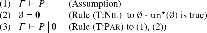
• Case $(\varvec{\nu }xy)P\mathord {\,\big |\,}Q \equiv _{\pi } (\varvec{\nu }xy)(P\mathord {\,\big |\,}Q)$ with $x,y\not \in \mathsf {fv}_{\pi }(Q)$:

  $\Rightarrow )$:

  

  We now distinguish two cases. The first (and most interesting) one is when $\texttt {un}^{\star }(T)$ is true. The second one corresponds to when $\texttt {un}^{\star }(T)$ is false (i.e., which groups the remaining possibilities):

  $\texttt {un}^{\star }(T)$ is true::

  We distinguish two further sub-cases depending on whether $\texttt {un}^{\star }(\overline{T})$ holds or not:

  $\texttt {un}^{\star }(\overline{T})$ is true::

  We apply Lemma 18 twice in (6) to obtain (7) $\varGamma _2, x:T, y:\overline{T} \vdash Q$ and conclude by applying ${(\textsc {T:Par})}$ and ${(\textsc {T:Res})}$ on (5) and (7).

  $\texttt {un}^{\star }(\overline{T})$ is false::

  We only apply weakening once (cf. Lemma 18) in (6) to obtain (7) $\varGamma _2, x:T \vdash Q$ and conclude by applying ${(\textsc {T:Par})}$ and ${(\textsc {T:Res})}$ to (5) and (7).

  $\texttt {un}^{\star }(T)$ is false::

  Then, $\texttt {lin}(T)$ holds; by Lemma 16(2), $\texttt {lin}(\overline{T})$ also holds. Thus, we distinguish two cases, depending on whether $\texttt {un}^{\star }(\overline{T})$ also holds or not. Each case proceeds similarly as above.

  $\Leftarrow )$:

  

  We distinguish two further cases depending on whether $\texttt {un}^{\star }(T)$ is true or false:

  $\texttt {un}^{\star }(T)$ is true::

  We distinguish two further sub-cases depending on whether the $\texttt {un}^{\star }(\overline{T})$ holds or not:

  $\texttt {un}^{\star }(\overline{T})$ is true::

  Then, by inversion on ${(\textsc {T:Par})}$ on (3), we have (4) $\varGamma , x:T, y: \overline{T} \vdash P$ and (5) $\varGamma _2, x:T, y:\overline{T} \vdash Q$. Then, we apply Rule ${(\textsc {T:Res})}$ on (4) to obtain (6) $\varGamma _1 \vdash (\varvec{\nu }xy)P$ and we apply Lemma 19(2) to (5), obtaining (7) $\varGamma _2 \vdash Q$. We conclude by applying Rule ${(\textsc {T:Par})}$ to (6) and (7).

  $\texttt {un}^{\star }(\overline{T})$ is false::

  Then, by inversion on ${(\textsc {T:Par})}$ on (3), we have (4) $\varGamma , x:T, y: \overline{T} \vdash P$ and (5) $\varGamma _2 \vdash Q$. Moreover, by Lemma 19(1) applied to (2) and (5), it must be the case that $y:\overline{T}\not \in \varGamma _2$. Therefore, we apply Lemma 19(2) once to remove x : T from $\varGamma _2$. Then, we apply Rule ${(\textsc {T:Res})}$ in (4) to obtain (6) $\varGamma \vdash (\varvec{\nu }xy)P$ and conclude by applying Rule ${(\textsc {T:Par})}$.

  $\texttt {un}^{\star }(T)$ is false::

  As previously described, from Lemma 16(2), we distinguish two cases depending on $\texttt {un}^{\star }(\overline{T})$. Each case proceeds similarly as above.

$\square$

Lemma 21

(Substitution) If $\varGamma _1 \vdash v:T$ and $\varGamma _2, x: T \vdash P$ then , with $\varGamma = \varGamma _1 \circ \varGamma _2$.

Proof

By induction on the structure of P. There are nine cases: one base case and eight inductive cases.

Base Case::

$P = \mathbf {0}$. By inversion, $\texttt {un}^{\star }(\varGamma _2, x:T)$, which implies $\texttt {un}^{\star }(T)$. By inversion on the rules for values, we also have that $\texttt {un}^{\star }(\varGamma _1)$. Thus, $\texttt {un}^{\star }(\varGamma )$, with $\varGamma = \varGamma _1 \circ \varGamma _2$ holds. Since , the proof concludes by applying Rule ${(\textsc {T:Nil})}$.

Inductive Step::

The proofs for $P = Q_1 \mathord {\,\big |\,}Q_2$, $P = (\varvec{\nu }yz)Q$, and $P = u?\,Q_1\!:\!Q_2$ follow by applying the IH. The other five cases proceed similarly. We only detail the case for $P = {y}\langle u\rangle .Q$.

$P = {y}\langle u\rangle .Q$::

We distinguish four sub-cases: (1) $y = x$ and $\lnot \texttt {un}^{\star }(T)$, (2) $y = x$ and $\texttt {un}^{\star }(T)$, (3) $u = x$ and $\lnot \texttt {un}^{\star }(T)$, (4) $u = x$ and $\texttt {un}^{\star }(T)$. We only detail sub-cases (1), (2) and (4) since sub-case (3) proceeds similarly to (1) and (4).

1.:

By assumption, $P = {x}\langle u\rangle .Q$ and $\lnot \texttt {un}^{\star }(T)$. Moreover, since judgment $\varGamma _2 \vdash P$ can only be obtained with Rule ${(\textsc {T:Out})}$, it must be the case that $T = q!U.U'$. Thus, by inversion on Rule ${(\textsc {T:Out})}$, (1) $\varGamma _2 = \varDelta _1 \circ \varDelta _2 \circ \varDelta _3$, (2) $\varDelta _1 \vdash x:q!U.U'$, (3) $\varDelta _2 \vdash u : U$, and (4) $\varDelta _3 + x:U' \vdash Q$. We distinguish two further cases depending on whether $q={{\,\mathrm{\texttt {lin}}\,}}$ or $q= {{\,\mathrm{\texttt {un}}\,}}$. We only show the case $q= {{\,\mathrm{\texttt {un}}\,}}$, as the other proceeds similarly. By (2), it must be the case that $x:T \in \varDelta _1$. Moreover, by inversion on (2) and (3), we have that $\texttt {un}^{\star }(\varDelta '_1)$ holds with (5) $\varDelta '_1 = \varDelta _1 \setminus x:T$, and that (6) $\texttt {un}^{\star }(\varDelta _2)$ holds. By Lemma 19(1), we also have that $x:T \not \in \varDelta _2$ and $x:T\not \in \varDelta _3$. Moreover, by Lemma 17(1), $\varDelta _3 = \varGamma _2$, which implies that $\varDelta _3 + x:U' = \varGamma _2,x:U'$. By applying the IH, 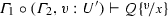. We then distinguish two further cases depending on whether $\texttt {un}^{\star }(U)$ or $\lnot \texttt {un}^{\star }(U)$. In both cases we proceed similarly: we add all the missing hypothesis applying Lemma 18 and conclude by reapplying Rule ${(\textsc {T:Out})}$.

2.:

This sub-case is not possible: by assumption, $\varGamma , x:T \vdash {x}\langle u\rangle .P$, which means that the judgment proceeds with Rule ${(\textsc {T:Out})}$. Thus, by inversion $T = {{\,\mathrm{\texttt {un}}\,}}!U.U'$. Now, by Definition 6, $\texttt {un}^{\star }(T)$ cannot hold, which contradicts the assumptions of this case (i.e., $y = x$ and $\texttt {un}^{\star }(T)$).

4.:

By assumption, $P = {y}\langle x\rangle .Q$ and $\texttt {un}^{\star }(T)$. Moreover, since judgment $\varGamma _2 \vdash P$ can only be obtained with Rule ${(\textsc {T:Out})}$, it must be the case that $T = q!U.U'$. We distinguish cases depending on whether $\texttt {un}^{\star }(U)$ or $\lnot \texttt {un}^{\star }(U)$ are true. Both cases proceed similarly, so we only detail the latter. If $\texttt {un}^{\star }(U)$ holds, we have that (1) $\varGamma _2 = \varDelta _1 \circ \varDelta _2 \circ \varDelta _3$, (2) $\varDelta _1 \vdash x:q!U.U'$, (3) $\varDelta _2 \vdash x : U$, and (4) $\varDelta _3 + y:U' \vdash P$, and $x:U \in \varDelta _1$, $x:U \in \varDelta _2$, and $x:U \in \varDelta _3$. Following a similar line of reasoning as the one above, we conclude that $\varDelta _3 = \varGamma _2$ and that $\varDelta _1 = \varDelta _2$. Moreover, by assumption $\varGamma _1 \vdash v:U$ and by IH . We then distinguish two further cases depending on whether $\texttt {un}^{\star }(U')$ or $\lnot \texttt {un}^{\star }(U')$. In both cases we conclude similarly as above.$\square$

Theorem 1

(Subject Reduction) If $\varGamma \vdash P$ and $P \longrightarrow Q$, then $\varGamma \vdash Q$.

Proof

By induction on the derivation of the reduction $P \longrightarrow Q$. The interesting cases are when the derivation stops with Rules ${\lfloor \textsc {Com}\rfloor }$ and ${\lfloor \textsc {Rep}\rfloor }$. The other cases proceed similarly; the case of Rule ${\lfloor \textsc {Str}\rfloor }$ follows by the IH and Lemma 20.

• Case ${\lfloor \textsc {Com}\rfloor }$:

  

  By Lemma 16(2), $\texttt {lin}(T)$ implies $\texttt {lin}(\overline{T})$. Thus, it is enough to distinguish cases depending on T and $\overline{T}$. We consider these combinations:

  • Case $\lnot \texttt {un}^{\star }(T)\wedge \lnot \texttt {un}^{\star }(\overline{T})$: We have that (a) $\varGamma _1,x:U' \vdash Q_1$, by (15) and the definition of $+$; (b) $\varGamma _2, z:U, y:\overline{U'} \vdash Q_2$, by (16) and the definition of $+$; (c) $\varGamma _3 \vdash Q_3$, by (8), and (d) $\varGamma ''_1 \vdash v:U$, by (11). By Lemma 21 (substitution) applied to (d) and (b), we have (e) $\varGamma _2, y:\overline{U'} \vdash Q_2$, and we can finish the proof by applying rules ${(\textsc {T:Par})}$, ${(\textsc {T:Par})}$, ${(\textsc {T:Res})}$.

  • Case $\lnot \texttt {un}^{\star }(T) \wedge \texttt {un}^{\star }(\overline{T})$: We have that (a) $\varGamma _1,x:U' \vdash Q_1$, by (15) and the definition of $+$; $(\varGamma _2, z:U') + y:\overline{U'} \vdash Q_2$ and $y:{{\,\mathrm{\texttt {un}}\,}}?U.\overline{U'}\in \varGamma _2$, by (16) and Definition of $\texttt {un}^{\star }(\cdot )$. Thus, $\overline{U'} = {{\,\mathrm{\texttt {un}}\,}}?U.\overline{U'}$ and thus, (b) $\varGamma _2, z:U',y:\overline{T} \vdash Q_2$. Similarly as above, we also have (c) $\varGamma _3 \vdash Q_3$, by (8); and (d) $\varGamma ''_1 \vdash v:U$, by (11). By Lemma 18 on (a), we have (e)  $\varGamma _1,x:U', y:\overline{T} \vdash Q_1$, and we can conclude by applying Lemma 21 and rules ${(\textsc {T:Par})}$, ${(\textsc {T:Par})}$, ${(\textsc {T:Res})}$ as above.

  • Other Cases: Notice that cases (i) $\texttt {un}^{\star }(T)\wedge \texttt {un}^{\star }(\overline{T})$ and (ii)  $\texttt {un}^{\star }(T) \wedge \lnot \texttt {un}^{\star }(\overline{T})$ are not possible, because $T = {{\,\mathrm{\texttt {un}}\,}}!U.U'$. Therefore, $\texttt {out}(T) = \texttt {tt}$ and the definition of $\texttt {un}^{\star }(T)$ (cf. Definition 6) would not hold.

• Case ${\lfloor \textsc {Rep}\rfloor }$: Assuming $P = (\varvec{\nu }xy)({x}\langle v\rangle .Q_1 \mathord {\,\big |\,}\mathbf {*}\, y(z).Q_2 \mathord {\,\big |\,}Q_3)$, we proceed similarly as above. By inversion on Rule ${(\textsc {T:Res})}$, $\varGamma , x: T, y:\overline{T} \vdash {x}\langle v\rangle .Q_1 \mathord {\,\big |\,}\mathbf {*}\, y(z).Q_2 \mathord {\,\big |\,}Q_3$, with $\varGamma = \varGamma _1 \circ \varGamma _2 \circ \varGamma _3$. Following a similar derivation as above, we conclude that $T = q!U.U'$, and $\overline{T} = q?U.\overline{U'}$. Then, we deduce:

  • (a) $\varGamma _1 = \varGamma '_1 \circ \varGamma ''_1 \circ \varGamma '''_1$;

  • (b) $\varGamma '''_1 + x:U' \vdash Q_1$, by inversion Rule ${(\textsc {T:Out})}$;

  • (c) $\varGamma ''_1, x:T \vdash x:q!U.U'$, by inversion Rule ${(\textsc {T:Out})}$;

  • (d) $\texttt {un}^{\star }(\varGamma ''_1)$, by inversion Rule ${(\textsc {T:Var})}$;

  • (e) $\varGamma ' \vdash v:U$, by inversion Rule ${(\textsc {T:Out})}$;

  • (f) $\texttt {un}^{\star }(\varGamma '_1)$, by inversion Rule ${(\textsc {T:Var})}$ (or ${(\textsc {T:Bool})}$);

  • (g) $(\varGamma _2, y:\overline{T}, z:U'') + y:\overline{U'} \vdash Q_2$, by inversion Rule ${(\textsc {T:Rin})}$;

  • (h) $\texttt {un}^{\star }(\varGamma _2, y:\overline{T}) \wedge (\texttt {un}^{\star }(U'')\vee U'' = {{\,\mathrm{\texttt {lin}}\,}}\,p)$, by inversion Rule ${(\textsc {T:Rin})}$;

  • (i) $\varGamma _3 \vdash Q_3$, by inversion Rule ${(\textsc {T:Par})}$.

  By (h), we have two possible cases:

  • Case $\texttt {un}^{\star }(\varGamma _2, y:\overline{T}) \wedge \texttt {un}^{\star }(U'')$: we have that $\texttt {un}^{\star }(\overline{T})$ holds, which implies: $\lnot \texttt {out}(\overline{T})$ and $\overline{T} = U'$ and $U'' = U$; hence T is a recursive type. Moreover, by Lemma 16(1b), we have that $\texttt {un}^{\star }(T)$ does not hold. Hence, we have that: $x:T \not \in \varGamma '''_1$, $x:T\not \in \varGamma '_1$. Then, by Lemma 17(1) to (a), (d), and (f), we have that $\varGamma '''_1 = \varGamma _1$. Then, by applying Lemma 21 and 18 to (e) and (c), we have that . We then apply Lemma 18 to (i) to obtain $(\varGamma _3, y:\overline{T}) \circ \varGamma '_1 \circ \varGamma ''_1 \vdash Q_3$. Notice that we also know, by Lemma 18, that $\varGamma '_1, \varGamma ''_1\circ (\varGamma _2, y:\overline{T}) \vdash \mathbf {*}\, y(z).Q_2$. We then apply Rule ${(\textsc {T:Par})}$ (which is applicable, since $\texttt {un}^{\star }(\overline{T})$ holds) to the previous hypotheses to obtain:

    $$\begin{aligned} \varGamma , x:T, y:\overline{T} \vdash Q_1 \mathord {\,\big |\,}Q_2 \mathord {\,\big |\,}\mathbf {*}\, y(z).Q_2 \mathord {\,\big |\,}Q_3 \end{aligned}$$

    We then conclude by applying Rule ${(\textsc {T:Res})}$.

  • Case $\texttt {un}^{\star }(\varGamma _2, y:\overline{T}) \wedge U'' = {{\,\mathrm{\texttt {lin}}\,}}\, p$: This case proceeds as above. The only difference is that the assumption implies that $v: {{\,\mathrm{\texttt {lin}}\,}}\,p$. This in turn means that $v: {{\,\mathrm{\texttt {lin}}\,}}\,p \not \in \varGamma _1'''$ and $v: {{\,\mathrm{\texttt {lin}}\,}}\,p \not \in \varGamma _1'$, which allows us to conclude with the same argument as above.

$\square$

Theorem 4

(Type Safety) If $\,\vdash P$, then P is well-formed.

Proof

For the sake of contradiction, assume that $\vdash P$ and P is not well-formed, i.e., it does not satisfy any of the three items in Definition 10. If $\vdash P$, then there exists a derivation

$$\begin{aligned} \vdash (\varvec{\nu }x_1\dots x_ny_1\dots y_n)(Q_1\mathord {\,\big |\,}Q_2 \mathord {\,\big |\,}R) \qquad \text {(with }n\ge 1) \end{aligned}$$

Therefore, by applying inversion n times, there exists a context $x_1: T_n, \dots , x_n:T_n, y_1:\overline{T}_1, \dots , y_n:\overline{T}_n = \varGamma _1 \circ \varGamma _2 \circ \varGamma _3$ that types $Q_1\mathord {\,\big |\,}Q_2 \mathord {\,\big |\,}R$. We now show that if $Q_1\mathord {\,\big |\,}Q_2 \mathord {\,\big |\,}R$ does not satisfy any item in Definition 10, then we reach a contradiction:

• 1. If $Q_1=v?\,Q_1\!:\!Q_2$ then $v\in \{\texttt {tt} ,\texttt {ff} \}$: Assume that does not satisfy this condition. Then, the derivation $\varGamma _1 \circ \varGamma _2 \circ \varGamma _3 \vdash Q_1\mathord {\,\big |\,}Q_2 \mathord {\,\big |\,}R$ is not possible as Rule ${(\textsc {T:If})}$ requires $v:\texttt {bool}$.

• 2. There are not $Q_1$ and $Q_2$ such that they are both prefixed with the same variable: Assume there exist $Q_1$ and $Q_2$ that are prefixed in the same variable. Then, there are two cases: (i) if the prefixes are of different nature, then we reach a contradiction: it is not possible for x : T and $x:T'$ with $T\not =T'$ to appear in a typing derivation in the same context; (ii) if the prefixes are of the same nature, we just need to notice that splitting does not allow for session types that satisfy $\texttt {out}(\cdot )$ to be shared among contexts (cf. Definition 8). Thus, only unrestricted input and branching types can be shared.

• 3. If $Q_1$ is prefixed on $x_1\in \widetilde{x}$ and $Q_2$ is prefixed on $y_1\in \widetilde{y}$ then $Q_1\mathord {\,\big |\,}Q_2$ is a redex: Suppose that this does not hold (i.e., $Q_1\mathord {\,\big |\,}Q_2$ is not a redex). Then, the typing derivation is not possible, since Rule ${(\textsc {T:Res})}$ requires the types of two covariables to be dual, thus reaching a contradiction.

$\square$

Appendix for Sect. 4

1.1 Junk processes

Lemma 2

Let J be junk. Then: (1) $J \mathop {\not \rightarrow }\limits ^{\tau }{}_{\ell }$ (and) (2) there is no $c\in \mathcal {C}$ (cf. Definition 21) such that $J \parallel \overline{c} \xrightarrow {\smash {\,\tau \,}}_{\ell }$.

Proof

We prove each item individually.

• (1) By induction on the structure of J. We show two cases:

  • Case $J = \mathbf {\forall }{\epsilon }((b = \lnot b) \rightarrow P)$: This case is immediate by inspecting the rules in Fig. 6; in particular, since Rule ${(\textsc {C:Sync})}$ cannot be applied $J \mathop {\not \rightarrow }\limits ^{\tau }{}_{\ell }$.

  • Case $J = J_1 \parallel J_2$: By IH, $J_1 \mathop {\not \rightarrow }\limits ^{\tau }{}_{\ell }$ and $J_2 \mathop {\not \rightarrow }\limits ^{\tau }{}_{\ell }$. We prove that a reduction $J_1 \parallel J_2 \xrightarrow {\smash {\,\tau \,}}_{\ell } J'_1 \parallel J'_2$ cannot occur. By Definition 28, junk processes are either ask-guarded processes or $\overline{\texttt {tt} }$. To reduce, one of $J_1$ and $J_2$ must add a constraint to the store; two parametric ask processes in parallel cannot reduce (cf. Fig. 6). Now, since $\overline{\texttt {tt} }$ does not add any information to the store, we have that $J_1 \parallel J_2 \mathop {\not \rightarrow }\limits ^{\tau }{}_{\ell }$.

• (2) By induction on the structure of J. We detail three cases:

  • Case $J = \overline{\texttt {tt}}$: This case is immediate, as $\overline{\texttt {tt} } \parallel \overline{c} \mathop {\not \rightarrow }\limits ^{\tau }{}_{\ell }$, for any constraint $c\in \mathcal {C}$.

  • Case $J = \mathbf {\forall }{\epsilon }((b = \lnot b) \rightarrow P)$: Suppose, for the sake of contradiction, that there is a $c\in \mathcal {C}$ (cf. Definition 21) such that $J \parallel \overline{c} \xrightarrow {\smash {\,\tau \,}}_{\ell } S$, for some S. Then, by Definition 21, c must be composed of the predicates $\mathsf {snd}$, $\mathsf {rcv}$, $\mathsf {sel}$, $\mathsf {bra}$, $\{\cdot {:}\cdot \}$ (cf. Fig. 7), the multiplicative conjunction $\otimes$, replication, and the existential quantifier. We now apply induction on the structure of c: there are five base cases (one for each predicate) and three inductive cases (one for each logical connective). We show only two representative cases:

    • Sub-case $c = \mathsf {snd} (x,v)$: This base case is immediate, as $\mathsf {snd} (x,v) \not \vdash (b = \lnot b)$ using the Rules in Fig. 5. Thus, Rule ${(\textsc {C:Sync})}$ is not applicable, therefore contradicting our assumption.

    • Sub-case $c = c_1 \otimes c_2$: By IH, $c_i \not \vdash (b = \lnot b)$. Then, by the rules in Fig. 5, $c_1 \otimes c_2 \not \vdash (b = \lnot b)$, leading to a contradiction as in the previous sub-case.

  • Case $J = J_1 \parallel J_2$: Then, $J \parallel \overline{c} \mathop {\not \rightarrow }\limits ^{\tau }{}_{\ell }$ follows immediately from the IH (which ensures $J_1 \parallel \overline{c} \mathop {\not \rightarrow }\limits ^{\tau }{}_{\ell }$ and $J_2 \parallel \overline{c} \mathop {\not \rightarrow }\limits ^{\tau }{}_{\ell }$) and Item (1).

$\square$

Lemma 3

(Junk Observables) For every junk process J and every $\mathcal {D}_{\pi }\mathcal {C}$-context $C[- ]$, we have that: (1) $\mathcal {O}^{\mathcal {D}_{\pi }}(J) = \emptyset$ (and) (2) $\mathcal {O}^{\mathcal {D}_{\pi }}(C[J ]) = \mathcal {O}^{\mathcal {D}_{\pi }}(C[\overline{\texttt {tt}} ])$.

Proof

We prove each item separately:

• 1. By induction on the structure of J. We show the most representative 3 cases:

  • Case $J= \mathbf {\forall }{\epsilon }((b = \lnot b) \rightarrow P)$: By Lemma 2(1), $J\mathop {\not \rightarrow }\limits ^{\tau }{}_{\ell }$. Therefore, by Definition 15$\mathcal {O}^{\mathcal {D}_{\pi }}(J) = \emptyset$.

  • Case $J= \overline{\texttt {tt}}$: By Lemma 2(1), $J\mathop {\not \rightarrow }\limits ^{\tau }{}_{\ell }$. Moreover, since $\texttt {tt}\not \in \mathcal {D}_{\pi }$, by Definition 15, $\mathcal {O}^{\mathcal {D}_{\pi }}(J) = \emptyset$.

  • Case $J = J_1 \parallel J_2$: By IH, $\mathcal {O}^{\mathcal {D}_{\pi }}(J_i) = \emptyset$, $i\in \{1,2\}$. By Lemma 2(1), $J\mathop {\not \rightarrow }\limits ^{\tau }{}_{\ell }$ and therefore, $\mathcal {O}^{\mathcal {D}_{\pi }}(J) = \mathcal {O}^{\mathcal {D}_{\pi }}(J_1) \cup \mathcal {O}^{\mathcal {D}_{\pi }}(J_2) = \emptyset$.

• 2. The proof is by induction on the structure of J, followed in each case by a case analysis on $C[- ]$ (cf. Definition 16). All cases follow from the definitions; we detail two representative cases:

  • Case $J = \mathbf {\forall }{\epsilon }((b = \lnot b) \rightarrow P_1)$: We apply a case analysis on context $C[- ]$. We will show only two sub-cases, as the third one is symmetrical:

    • Sub-case $C[- ] = \exists \widetilde{x}. \, -$: This case follows immediately from Lemma 2(1,2).

    • Sub-case $C[- ] = - \parallel P_2$: Then $C[J ] = \mathbf {\forall }{\epsilon }((b = \lnot b) \rightarrow P_1) \parallel P_2$. By Lemma 2(1,2), $\mathbf {\forall }{\epsilon }((b = \lnot b) \rightarrow P_1) \mathop {\not \rightarrow }\limits ^{\tau }{}_{\ell }$ and there is no $c\in \mathcal {C}$ (cf. Definition 21) such that $J \parallel \overline{c} \xrightarrow {\smash {\,\tau \,}}_{\ell }$. As such, a reduction is not possible (i.e., J cannot reduce in the context). Therefore, by Definition 15 and Item (1), $\mathcal {O}^{\mathcal {D}_{\pi }}(C[J ]) = \mathcal {O}^{\mathcal {D}_{\pi }}(J) \cup \mathcal {O}^{\mathcal {D}_{\pi }}(P_2) = \mathcal {O}^{\mathcal {D}_{\pi }}(P_2)$. Following a similar analysis, and using Lemma 2(1,2), Item(1) and Definition 15, we have that $\mathcal {O}^{\mathcal {D}_{\pi }}(C[ \overline{\texttt {tt}}]) = \mathcal {O}^{\mathcal {D}_{\pi }}(\overline{\texttt {tt}}) \cup \mathcal {O}^{\mathcal {D}_{\pi }}(P_2) = \mathcal {O}^{\mathcal {D}_{\pi }}(P_2)$. We conclude $\mathcal {O}^{\mathcal {D}_{\pi }}(C[ \overline{\texttt {tt}}]) = \mathcal {O}^{\mathcal {D}_{\pi }}(C[J ])$, as wanted.

  • Case $J = J_1 \parallel J_2$: We apply a case analysis on context $C[- ]$. We will show only two sub-cases, as the third one is symmetrical:

    • Sub-case $C[- ] = \exists \widetilde{x}. \big (- \big )$: This case follows immediately from Lemma 2(1,2).

    • Sub-case $C[- ] = - \parallel P_2$: By IH, we have $\mathcal {O}^{\mathcal {D}_{\pi }}(C[J_1 ]) = \mathcal {O}^{\mathcal {D}_{\pi }}(C[ \overline{\texttt {tt}}])$ and $\mathcal {O}^{\mathcal {D}_{\pi }}(C[J_2])$ $=$ $\mathcal {O}^{\mathcal {D}_{\pi }}(C[ \overline{\texttt {tt}}])$. Also, by Lemma 2(1), $J_1 \parallel J_2 \mathop {\not \rightarrow }\limits ^{\tau }{}_{\ell }$ and by Lemma 2(2), there is no $c\in \mathcal {C}$ (cf. Definition 21) such that $J \parallel \overline{c} \xrightarrow {\smash {\,\tau \,}}_{\ell }$. Hence, by Definition 15 and Item (1), $\mathcal {O}^{\mathcal {D}_{\pi }}(C[J_1 \parallel J_2]) = \mathcal {O}^{\mathcal {D}_{\pi }}(\overline{\texttt {tt}})$, as wanted.

$\square$

Lemma 4

(Junk Behavior) For every junk J, every $\mathcal {D}_{\pi }\mathcal {C}$-context $C[ - ]$, and every process P, we have $C[ P \parallel J ] \approx ^{\pi }_\ell C[ P ]$.

Proof

By coinduction, i.e., by exhibiting a weak o-barbed bisimulation containing the pair $(C[P \parallel J ], C[ P ])$. To build the needed bisimulation, we recall Definition 17. That is, we must define a symmetric relation $\mathcal {R}$ such that $(R, Q) \in \mathcal {R}$ implies:

• 1. $\mathcal {O}^{\mathcal {D}_{\pi }}(R) = \mathcal {O}^{\mathcal {D}_{\pi }}(Q)$ (and),

• 2. whenever $R\xrightarrow {\smash {\,\tau \,}}_{\ell } R'$ there exists $Q'$ such that and $R'\mathcal {R}Q'$.

Then, let us consider:

$$\begin{aligned} \mathcal {R}&= \{(R,Q) \, {\mid }\,C[P \parallel J ] \xrightarrow {\smash {\,\tau \,}}_{\ell } ^{n} R \wedge C[P] \xrightarrow {\smash {\,\tau \,}}_{\ell } ^{n} Q, n\ge 0\} \\&\cup \, \{(Q,R) \, {\mid }\,C[P \parallel J ] \xrightarrow {\smash {\,\tau \,}}_{\ell } ^{n} R \wedge C[P] \xrightarrow {\smash {\,\tau \,}}_{\ell } ^{n} Q, n\ge 0\} \end{aligned}$$

(1)

Observe that $\mathcal {R}$ is symmetric by definition. Moreover, it immediately satisfies Item (1) thanks to Lemma 3(2).

As for Item (2), first notice that $(R, Q) \in \mathcal {R}$: we have $R = C[P\parallel J]$ and $Q = C[P]$ (with $n=0$). Now suppose that $R \xrightarrow {\smash {\,\tau \,}}_{\ell } R'$; we show a matching transition such that $R'\mathcal {R}Q'$. To this end, we use a case analysis on the reduction(s) possible from $C[P \parallel J ]$. There are six possibilities:

• (a) $C[P \parallel J ] \xrightarrow {\smash {\,\tau \,}}_{\ell } C[P \parallel J']$ (i.e., an autonomous reduction from J);

• (b) $C[P \parallel J ] \xrightarrow {\smash {\,\tau \,}}_{\ell } C'[P \parallel J']$ (i.e., a reduction from the interplay of C and J);

• (c) $C[P \parallel J ] \xrightarrow {\smash {\,\tau \,}}_{\ell } C[P' \parallel J']$ (i.e., a reduction from the interplay of P and J);

• (d) $C[P \parallel J ] \xrightarrow {\smash {\,\tau \,}}_{\ell } C'[P \parallel J]$ (i.e., an autonomous reduction from C);

• (e) $C[P \parallel J ] \xrightarrow {\smash {\,\tau \,}}_{\ell } C'[P' \parallel J]$ (i.e., an interaction between C and P);

• (f) $C[P \parallel J ] \xrightarrow {\smash {\,\tau \,}}_{\ell } C[P' \parallel J]$ (i.e., an autonomous reduction from P).

Notice that Lemma 2(1,2) and Lemma 3(1,2) exclude cases (a)–(c). Thus, reductions for C[J] will only be of the form (d)–(f). Clearly, this transition from R can be matched by Q as follows:

• $Q = C[P ] \xrightarrow {\smash {\,\tau \,}}_{\ell } C'[P] = Q'$, with $(C'[P \parallel J], C'[P]) \in \mathcal {R}$ (or)

• $Q = C[P ] \xrightarrow {\smash {\,\tau \,}}_{\ell } C'[P'] = Q'$, with $(C'[P' \parallel J], C'[P']) \in \mathcal {R}$ (or)

• $Q = C[P ] \xrightarrow {\smash {\,\tau \,}}_{\ell } C[P'] = Q'$, with $(C[P' \parallel J], C[P']) \in \mathcal {R}$.

With these reductions, we conclude the proof for this case. The case when $Q \xrightarrow {\smash {\,\tau \,}}_{\ell } Q'$ is similar. $\square$

Lemma 5

(Occurrences of Junk) Let R be a redex (Definition 9).

• 1. If $R = x \triangleleft l_j.P \mathord {\;|\;}y \triangleright \{l_i:Q_i\}_{i\in I}$, with $j \in I$ then:

  $\llbracket (\varvec{\nu }xy)R \rrbracket \xrightarrow {\smash {\,\tau \,}}_{\ell } ^3 \exists x,y. \big ({{\,\mathrm{!}\,}}\overline{\{x{:}y\}}\parallel \llbracket P \rrbracket \parallel \llbracket Q_j \rrbracket \parallel J\big )$, where

  $J = \prod \limits _{i\in I'}\mathbf {\forall }{\epsilon }(l_j=l_i \rightarrow \llbracket Q_i \rrbracket )$, with $I' = I\setminus \{j\}$, and

  $\exists x,y. \big ({{\,\mathrm{!}\,}}\overline{\{x{:}y\}}\parallel \llbracket P \rrbracket \parallel \llbracket Q_j \rrbracket \parallel J\big ) \cong ^{\pi }_\ell \exists x,y. \big ({{\,\mathrm{!}\,}}\overline{\{x{:}y\}}\parallel \llbracket P \rrbracket \parallel \llbracket Q_j \rrbracket \big ).$

• 2. If $R = b?\,P_1\!:\!P_2$, $b\in \{\texttt {tt} ,\texttt {ff} \}$, then:

  $\llbracket R \rrbracket \xrightarrow {\smash {\,\tau \,}}_{\ell } \llbracket P_i \rrbracket \parallel J$, $i\in \{1,2\}$ with $J = \mathbf {\forall }{\epsilon }(b = \lnot b \rightarrow \llbracket P_j \rrbracket )$, $j\ne i$, and

  $\llbracket P_i \rrbracket \parallel J \cong ^{\pi }_\ell \llbracket P_i \rrbracket$.

• 3. If $R = {x}\langle v\rangle .P \mathord {\;|\;}y(z).Q$, then

  with $J= \overline{\texttt {tt}}$.

• 4. If $R = {x}\langle v\rangle .P \mathord {\;|\;}\mathbf {*}\, y(z).Q$ then:

  

Proof

Each item follows from the definition of $\llbracket \cdot \rrbracket$ (cf. Definition 25 and Fig. 8). Items (1) and (2) refer to reductions that induce junk (no junk is generated in Items (3) and (4)); those cases rely on the definition of weak o-barbed congruence (cf. Definition 23) and Corollary 2.

• 1. Given $R = x \triangleleft l_j.P \mathord {\;|\;}y \triangleright \{l_i:Q_i\}_{i\in I}$ (with $j \in I$), by Definition 25, Fig. 8, and the operational semantics of $\texttt {lcc}$ in Definition 6:

  $$\begin{aligned} \llbracket (\varvec{\nu }xy)R \rrbracket&= \exists x,y. \big (!\overline{\{x{:}y\}} \parallel \overline{\mathsf {sel} (x,l_j)} \parallel \mathbf {\forall }{z}\big (\mathsf {bra} (z,l_j)\otimes \{x{:}z\} \rightarrow \llbracket P \rrbracket \big ) \\&\qquad \qquad \,\,\mathbf {\forall }{l,w}\big (\mathsf {sel} (w,l) \otimes \{w{:}x\} \rightarrow \overline{\mathsf {bra} (x,l)}\parallel \prod \limits _{i\in I} \mathbf {\forall }{\epsilon }(l=l_i \rightarrow \llbracket Q_i \rrbracket ) \big ) \big )\\&\xrightarrow {\smash {\,\tau \,}}_{\ell } \exists x,y. \big (!\overline{\{x{:}y\}} \parallel \mathbf {\forall }{z}\big (\mathsf {bra} (z,l_j)\otimes \{x{:}z\} \rightarrow \llbracket P \rrbracket \big ) \\&\qquad \qquad \,\,\overline{\mathsf {bra} (x,l_j)}\parallel \prod \limits _{i\in I} \mathbf {\forall }{\epsilon }(l_j=l_i \rightarrow \llbracket Q_i \rrbracket ) \big )\\&\xrightarrow {\smash {\,\tau \,}}_{\ell } \exists x,y. \big (!\overline{\{x{:}y\}} \parallel {\llbracket P \rrbracket } \parallel \prod \limits _{i\in I} \mathbf {\forall }{\epsilon }(l_j=l_i \rightarrow \llbracket Q_i \rrbracket ) \big )\\&\xrightarrow {\smash {\,\tau \,}}_{\ell } \exists x,y. \big (!\overline{\{x{:}y\}} \parallel {\llbracket P \rrbracket } \parallel \llbracket P_j \rrbracket \parallel \underbrace{\prod \limits _{i \in I\setminus \{j\}} \mathbf {\forall }{\epsilon }(l_j=l_i \rightarrow \llbracket Q_i \rrbracket )}_{J} \big ) \\&\cong ^{\pi }_\ell \exists x,y. \big (!\overline{\{x{:}y\}} \parallel {\llbracket P \rrbracket } \parallel \llbracket P_j \rrbracket \big ) \end{aligned}$$

  where the last step is justified by Corollary 2.

• 2. Given that $R = b?\,P_1\!:\!P_2$, we distinguish two cases: $b = \texttt {tt}$ and $b = \texttt {ff}$. We only detail the analysis when $R = \texttt {tt} ?\,P_1\!:\!P_2$, as the other case is analogous. By the translation definition (cf. Definition 25 and Fig. 8), $\llbracket R \rrbracket = \mathbf {\forall }{\epsilon }(\texttt {tt}=\texttt {tt} \!\rightarrow \! \llbracket P_1 \rrbracket ) \parallel \mathbf {\forall }{\epsilon }(\texttt {tt}= \texttt {ff} \!\rightarrow \! \llbracket P_2 \rrbracket )$. Then, by the rules in Fig. 6, $\llbracket R \rrbracket \xrightarrow {\smash {\,\tau \,}}_{\ell } \llbracket P_1 \rrbracket \parallel J$, with $J = \mathbf {\forall }{\epsilon }(\texttt {tt}= \texttt {ff} \!\rightarrow \! \llbracket P_2 \rrbracket )$. By Corollary 2, we may conclude as follows:

  $$\begin{aligned} \llbracket R \rrbracket \xrightarrow {\smash {\,\tau \,}}_{\ell } \llbracket P \rrbracket \parallel \mathbf {\forall }{\epsilon }(\texttt {tt}= \texttt {ff} \!\rightarrow \! \llbracket Q \rrbracket ) \cong ^{\pi }_\ell \llbracket P \rrbracket \end{aligned}$$

• 3. Given $R = {x}\langle v\rangle .P \mathord {\;|\;}y(z).Q$, by the translation definition (cf. Fig. 8), and the semantics in Fig. 6:

  

  Let $J = \overline{\texttt {tt}}$. Finally, we conclude by Corollary 2.

• 4. When $R = {x}\langle v\rangle .Q \mathord {\;|\;}\mathbf {*}\, y(z).P$, the proof follows the same reasoning as above.

$\square$

1.2 Operational completeness

Theorem 11

(Completeness for $\llbracket \cdot \rrbracket$) Let $\llbracket \cdot \rrbracket$ be the translation in Definition 25. Also, let P be a well-typed $\pi$ program. Then, if $P \longrightarrow ^{*} Q$, then .

Proof

By induction on the length of the reduction $\longrightarrow ^{*}$, with a case analysis on the last applied rule. The base case is when $P\longrightarrow ^0 P$: it is trivially true since . For the inductive step, assume by IH that $P\longrightarrow ^{*} P_0 \longrightarrow Q$ and . We then have to prove that . There are nine cases, since cases for Rules ${(\textsc {Res})}$, ${(\textsc {Par})}$ and ${(\textsc {Str})}$ are immediate by IH.

• Rule ${\lfloor \textsc {IfT}\rfloor }$:

  • (i) $P_0= \texttt {tt} ?\,P'\!:\!P''$.

  • (ii) By (i), $P_0 \longrightarrow P' = Q$.

  • (iii) By Definition 25, $\llbracket P_0 \rrbracket = \mathbf {\forall }{\epsilon }(\texttt {tt}= \texttt {tt} \rightarrow \llbracket P' \rrbracket ) \parallel \mathbf {\forall }{\epsilon }(\texttt {tt}= \texttt {ff} \rightarrow \llbracket P'' \rrbracket )$.

  • (iv) By Rule ${(\textsc {C:Sync})}$ (cf. Fig. 6), with $c = \texttt {tt}$ we have the following (note that $\Vdash \texttt {tt}= \texttt {tt}$):

    $$\begin{aligned} \llbracket P_0 \rrbracket \xrightarrow {\smash {\,\tau \,}}_{\ell } \llbracket P' \rrbracket \parallel \mathbf {\forall }{\epsilon }(\texttt {tt}= \texttt {ff} \rightarrow \llbracket P'' \rrbracket ) = R \end{aligned}$$

  • (v) By (iv) note that the process $\mathbf {\forall }{\epsilon }(\texttt {tt}= \texttt {ff} \rightarrow \llbracket P'' \rrbracket )$ is junk (cf. Definition 28). Then, by Corollary 2$R\cong ^{\pi }_\ell \llbracket Q \rrbracket$, which is what we wanted to prove.

• Rule ${\lfloor \textsc {IfF}\rfloor }$: Analogous to the previous case.

• Rule ${\lfloor \textsc {Com}\rfloor }$:

  • (i) $P_0 = (\varvec{\nu }xy)({x}\langle v\rangle .P' \mathord {\;|\;}y(z).P'' \mathord {\;|\;}T)$, with T corresponding to a parallel composition of processes that may contain y. Notice that by typing, T can only contain (replicated) input processes on y and not any processes containing x.

  • (ii) By (i) .

  • (iii) By Fig. 8:

    $$\begin{aligned} \llbracket P_0 \rrbracket&=\exists x,y. \big (\overline{{{\,\mathrm{!}\,}}\{x{:}y\}} \parallel \overline{(\mathsf {snd} (x,v)} \parallel \mathbf {\forall }{z_1}((\mathsf {rcv} (z_1,v)\otimes \{x{:}z_1\}) \rightarrow \llbracket P' \rrbracket ) \parallel \\&\qquad \quad \qquad \mathbf {\forall }{z_2,w}(\mathsf {snd} (w,z_2)\otimes \{w{:}y\}) \rightarrow (\overline{\mathsf {rcv} (y,z_2)} \parallel \llbracket P'' \rrbracket ) \parallel \llbracket T \rrbracket \big ) \end{aligned}$$

  • (iv) By Fig. 6, Definition 13:

    

  • (v) By Fig. 8 we have that $w\not \in \mathsf {fv}_{\pi }(P'')$ and $z_1\not \in \mathsf {fv}_{\pi }(P')$. Therefore:

    

  • (vi) Finally, by reflexivity of $\cong ^{\pi }_\ell$ (Definition 23), $\llbracket Q \rrbracket \cong ^{\pi }_\ell \llbracket Q \rrbracket$.

• Rule ${\lfloor \textsc {Repl}\rfloor }$:

  • (i) Assume $P_0 = (\varvec{\nu }xy)({x}\langle v\rangle .P' \mathord {\;|\;}\mathbf {*}\, y(z).P'' \mathord {\;|\;}T)$, with T collecting all the processes that may contain x and y. Notice that by typing, T can only contain (replicated) input processes on y.

  • (ii) By (i) using Rule ${\lfloor \textsc {Rep}\rfloor }$.

  • (iii) By definition of $\llbracket \cdot \rrbracket$:

    $$\begin{aligned} \llbracket P_0 \rrbracket&=\exists x,y. \big (\overline{!\{x{:}y\}} \parallel \overline{(\mathsf {snd} (x,v)} \parallel \mathbf {\forall }{z_1}((\mathsf {rcv} (z_1,v)\otimes \{x{:}z_1\}) \rightarrow \llbracket P' \rrbracket ) \parallel \\&\qquad \quad \qquad !\mathbf {\forall }{z_2,w}(\mathsf {snd} (w,z_2)\otimes \{w{:}y\}) \rightarrow (\overline{\mathsf {rcv} (y,z_2)} \parallel \llbracket P'' \rrbracket ) \parallel \llbracket T \rrbracket \big )\\&\equiv \exists x,y. \big (\overline{!\{x{:}y\}} \parallel \overline{(\mathsf {snd} (x,v)} \parallel \mathbf {\forall }{z_1}((\mathsf {rcv} (z_1,v)\otimes \{x{:}z_1\}) \rightarrow \llbracket P' \rrbracket ) \parallel \\&\qquad \quad \qquad \mathbf {\forall }{z_2,w}(\mathsf {snd} (w,z_2)\otimes \{w{:}y\}) \rightarrow (\overline{\mathsf {rcv} (y,z_2)} \parallel \llbracket P'' \rrbracket )) \parallel \\&\qquad \quad \qquad !\mathbf {\forall }{z_2,w}(\mathsf {snd} (w,z_2)\otimes \{w{:}y\}) \rightarrow (\overline{\mathsf {rcv} (y,z_2)} \parallel \llbracket P'' \rrbracket ) \parallel \llbracket T \rrbracket \big ) \end{aligned}$$

  • (iv) Let $R = \, !\mathbf {\forall }{z_2,w}(\mathsf {snd} (w,z_2)\otimes \{w{:}y\}) \rightarrow (\overline{\mathsf {rcv} (y,z_2)} \parallel \llbracket P'' \rrbracket ))$. By using the rules of structural congruence and reduction of $\texttt {lcc}$, the following transitions can be shown:

    

  • (v) As in Case ${\lfloor \textsc {Com}\rfloor }$, we have that

    

    since $w\not \in \mathsf {fv}_{\pi }(P'')$ and $z_1\not \in \mathsf {fv}_{\pi }(P'')$, by Fig. 8.

  • (vi) Finally, observe that:

    

• Rule ${\lfloor \textsc {Sel}\rfloor }$:

  • (i) Assume $P_0 = (\varvec{\nu }xy)(x \triangleleft l_j.P' \mathord {\;|\;}y \triangleright \{l_i:P_i\}_{i\in I} \mathord {\;|\;}T)$. Notice that since $P_0$ is a well-formed program, typing implies that process $T\equiv \mathbf {0}$, since x, y cannot be shared. Thus, we do not consider T below.

  • (ii) By (i) $P_0 \longrightarrow (\varvec{\nu }xy)(P' \mathord {\;|\;}P_j) = Q$ using Rule ${\lfloor \textsc {Sel}\rfloor }$.

  • (iii) By definition of $\llbracket \cdot \rrbracket$ (cf. Fig. 8):

    $$\begin{aligned} \llbracket P_0 \rrbracket&= \exists x,y. \big (!\overline{\{x{:}y\}} \parallel \overline{\mathsf {sel} (x,l_j)} \parallel \mathbf {\forall }{z}\big (\mathsf {bra} (z,l_j)\otimes \{x{:}z\} \rightarrow \llbracket P' \rrbracket \big ) \\&\qquad \qquad \,\,\mathbf {\forall }{l,w}\big (\mathsf {sel} (w,l) \otimes \{w{:}x\} \rightarrow \overline{\mathsf {bra} (x,l)}\parallel \prod \limits _{i\in I} \mathbf {\forall }{\epsilon }(l=l_i \rightarrow \llbracket P_i \rrbracket ) \big ) \big ) \end{aligned}$$

  • (iv) By using the semantics of $\texttt {lcc}$ (cf. Definition 6) and Corollary 2, we obtain the following derivation

    $$\begin{aligned} \llbracket P_0 \rrbracket&\xrightarrow {\smash {\,\tau \,}}_{\ell } \exists x,y. \big (!\overline{\{x{:}y\}} \parallel \mathbf {\forall }{z}\big (\mathsf {bra} (z,l_j)\otimes \{x{:}z\} \rightarrow \llbracket P' \rrbracket \big ) \\&\qquad \qquad \,\,\overline{\mathsf {bra} (x,l_j)}\parallel \prod \limits _{i\in I} \mathbf {\forall }{\epsilon }(l_j=l_i \rightarrow \llbracket P_i \rrbracket ) \big )\\&\xrightarrow {\smash {\,\tau \,}}_{\ell } \exists x,y. \big (!\overline{\{x{:}y\}} \parallel {\llbracket P' \rrbracket } \parallel \prod \limits _{i\in I} \mathbf {\forall }{\epsilon }(l_j=l_i \rightarrow \llbracket P_i \rrbracket ) \big )\\&\xrightarrow {\smash {\,\tau \,}}_{\ell } \exists x,y. \big (!\overline{\{x{:}y\}} \parallel {\llbracket P' \rrbracket } \parallel \llbracket P_j \rrbracket \parallel \underbrace{\prod \limits _{i \in I\setminus \{j\}} \mathbf {\forall }{\epsilon }(l_j=l_i \rightarrow \llbracket P_i \rrbracket )}_{J} \big ) \\&\cong ^{\pi }_\ell \exists x,y. \big (!\overline{\{x{:}y\}} \parallel {\llbracket P' \rrbracket } \parallel \llbracket P_j \rrbracket \big ) \end{aligned}$$

  • (v) By definition of $\llbracket \cdot \rrbracket$ (cf. Fig. 8), $\llbracket Q \rrbracket = \llbracket (\varvec{\nu }xy)(P' \mathord {\;|\;}P_j) \rrbracket = \exists x,y. \big (!\overline{\{x{:}y\}} \parallel {\llbracket P' \rrbracket } \parallel \llbracket P_j \rrbracket \big )$.

  • (vi) By (iv) and (v) we conclude the proof.

$\square$

1.3 Invariants for pre-redexes and redexes

Lemma 6

(Invariants of $\llbracket \cdot \rrbracket$ for Pre-Redexes and the Inaction) Let P be a pre-redex or the inactive process in $\pi$. Then, the following properties hold:

• 1. If $\,\mathcal {I}^\mathcal {\mathcal {D}^{\star }_{\pi }}(\llbracket P \rrbracket ) = \{\mathsf {snd} (x,v)\}$, then $P = {x}\langle v\rangle .P_1$, for some $P_1$.

• 2. If $\, \mathcal {I}^\mathcal {\mathcal {D}^{\star }_{\pi }}(\llbracket P \rrbracket )= \{\mathsf {sel} (x,l)\}$, then $P = x \triangleleft l.P_1$, for some $P_1$.

• 3. If $\,\mathcal {I}^\mathcal {\mathcal {D}^{\star }_{\pi }}(\llbracket P \rrbracket ) = \{\texttt {tt}\}$, then $P = \mathbf {0}$.

• 4. If $\,\mathcal {I}^\mathcal {\mathcal {D}^{\star }_{\pi }}(\llbracket P \rrbracket )= \emptyset$, then $P = \diamond ~y(z).P_1$ (cf. Notation 2) or $P = x \triangleright \{l_1:P_i\}_{i\in I}$, for some $P_i$. Moreover, $\llbracket P \rrbracket \mathop {\not \rightarrow }\limits ^{\tau }{}_{\ell }$.

Proof

By assumption $P = \mathbf {0}$ or P is a pre-redex (Definition 9): $P = {x}\langle v\rangle .P_1$, $P = x \triangleleft l.P_1$, $P = y(z).P_1$, $P = *y(z).P_1$ or $P = x \triangleright \{l_1:P_i\}_{i\in I}$. Given these six possible forms for P, we then check the immediate observables (cf. Definition 29) of their $\texttt {lcc}$ translations (cf. Fig. 8):

$$\begin{aligned} \mathcal {I}^\mathcal {\mathcal {D}^{\star }_{\pi }}(\llbracket {x}\langle v\rangle .P_1 \rrbracket )&= \{\mathsf {snd} (x,v)\}&\mathcal {I}^\mathcal {\mathcal {D}^{\star }_{\pi }}(\llbracket x(y).P_1 \rrbracket )&= \emptyset \\ \mathcal {I}^\mathcal {\mathcal {D}^{\star }_{\pi }}(\llbracket x \triangleleft l.P_1 \rrbracket )&= \{\mathsf {sel} (x,l)\}&\mathcal {I}^\mathcal {\mathcal {D}^{\star }_{\pi }}(\llbracket \mathbf {*}\, x(y).P_1 \rrbracket )&= \emptyset \\ \mathcal {I}^\mathcal {\mathcal {D}^{\star }_{\pi }}(\llbracket \mathbf {0} \rrbracket )&= \{\texttt {tt}\}&\mathcal {I}^\mathcal {\mathcal {D}^{\star }_{\pi }}(\llbracket x \triangleright \{l_1:P_i\}_{i\in I} \rrbracket )&= \emptyset \end{aligned}$$

This way, the thesis holds.$\square$

Lemma 7

(Invariants of $\llbracket \cdot \rrbracket$ for Input-Like Pre-Redexes) Let P be a pre-redex such that $\mathcal {I}^{\mathcal {D}^{\star }_{\pi }}(\llbracket P \rrbracket )$ $=$ $\emptyset$. Then, one of the following holds:

• 1. If $\llbracket P \rrbracket \parallel \overline{\mathsf {sel} (x,l_j)\otimes \{y{:}x\}} \xrightarrow {\smash {\,\tau \,}}_{\ell } S$, then

  $\mathsf {bra} (y,l_j) \in \mathcal {I}^{\mathcal {D}^{\star }_{\pi }}(S)$ and $P = y \triangleright \{l_i:P_i\}_{i\in I}$, with $j\in I$.

• 2. If $\llbracket P \rrbracket \parallel \overline{\mathsf {snd} (x,v)\otimes \{y{:}x\}} \xrightarrow {\smash {\,\tau \,}}_{\ell } S$, then $\mathsf {rcv} (y,v) \in \mathcal {I}^{\mathcal {D}^{\star }_{\pi }}(S)$ and $P = \diamond ~y(z).P_1$.

Proof

By assumption, P is a pre-redex and $\mathcal {I}^\mathcal {\mathcal {D}^{\star }_{\pi }}(P)=\emptyset$. By Lemma 6(4), we have that $\llbracket P \rrbracket \mathop {\not \rightarrow }\limits ^{\tau }{}_{\ell }$ and that $P = y(z).P_1$, $P = \mathbf {*}\, y(z).P_1$ or $P = y \triangleright \{l_1:P_i\}_{i\in I}$. We now apply a case analysis on each numeral in the statement:

• Case $\llbracket P \rrbracket \parallel \overline{\mathsf {sel} (w,l)\otimes \{y{:}x\}} \xrightarrow {\smash {\,\tau \,}}_{\ell } S$: We observe the behavior of each possibilities for P in the presence of constraint $\mathsf {sel} (w,l_j)\otimes \{y{:}x\}$ for some $l_j$, following Fig. 8. First, we observe:

  $$\begin{aligned} \llbracket y(z).P_1 \rrbracket \parallel \overline{\mathsf {sel} (w,l)\otimes \{y{:}x\}} =&\mathbf {\forall }{z,w}\big (\mathsf {snd} (w,z)\otimes \{w{:}y\} \!\rightarrow \! \overline{\mathsf {rcv} (y,z)} \parallel \llbracket P_1 \rrbracket \big ) \parallel \\&\overline{\mathsf {sel} (x,l_j)\otimes \{y{:}x\}} \mathop {\not \rightarrow }\limits ^{\tau }{}_{\ell } \\ \llbracket \mathbf {*}\, y(z).P_1 \rrbracket \parallel \overline{\mathsf {sel} (w,l)\otimes \{y{:}x\}} =&!(\mathbf {\forall }{z,w}\big (\mathsf {snd} (w,z)\otimes \{w{:}y\} \!\rightarrow \! \overline{\mathsf {rcv} (y,z)} \parallel \llbracket P_1 \rrbracket \big )) \parallel \\&\overline{\mathsf {sel} (x,l_j)\otimes \{y{:}x\}} \mathop {\not \rightarrow }\limits ^{\tau }{}_{\ell } \end{aligned}$$

  In contrast, process $\llbracket y \triangleright \{l_1:P_i\}_{i\in I} \rrbracket \parallel \overline{\mathsf {sel} (w,l)\otimes \{y{:}x\}}$ can reduce: from the semantics of $\texttt {lcc}$ (cf. Fig. 6) and under the assumption that $j\in I$ for $l_j$, we have:

  $$\begin{aligned}&\mathbf {\forall }{l,w}\big (\mathsf {sel} (w,l) \otimes \{w{:}y\} \rightarrow \overline{\mathsf {bra} (y,l)}\parallel \prod \limits _{1\le i \le n} \mathbf {\forall }{\epsilon }(l=l_i \rightarrow \llbracket P_i \rrbracket ) \big ) \parallel \overline{\mathsf {sel} (x,l_j)\otimes \{y{:}x\}} \\&\xrightarrow {\smash {\,\tau \,}}_{\ell } { \overline{\mathsf {bra} (y,l_j)}\parallel \prod \limits _{1\le i \le n} \mathbf {\forall }{\epsilon }(l=l_i \rightarrow \llbracket P_i \rrbracket )} = S \end{aligned}$$

  Finally, by Definition 29: $\mathcal {I}^\mathcal {\mathcal {D}^{\star }_{\pi }}(S) = \{\mathsf {bra} (y,l_j)\} \cup \mathcal {I}^\mathcal {\mathcal {D}^{\star }_{\pi }}(\prod \limits _{1\le i \le n} \mathbf {\forall }{\epsilon }(l_j=l_i \rightarrow \llbracket P_i \rrbracket ))$, thus concluding the proof.

• Case $\llbracket P \rrbracket \parallel \overline{\mathsf {snd} (x,v)\otimes \{y{:}x\}} \xrightarrow {\smash {\,\tau \,}}_{\ell } S$: This case proceeds as above by noticing that a reduction into S is enabled only when $P = y(z).P_1$ or $P = \mathbf {*}\, y(z).P_1$.

$\square$

Lemma 8

(Invariants for Redexes and Intermediate Redexes) Let R be a redex enabled by $\widetilde{x},\widetilde{y}$, such that $(\varvec{\nu }\widetilde{x}\widetilde{y})R \longrightarrow (\varvec{\nu }\widetilde{x}\widetilde{y})R'$. Then, one of the following holds:

• 1. If $R\equiv _{\pi } v?\,P_1\!:\!P_2$ and $v\in \{\texttt {tt} ,\texttt {ff} \}$, then

  $\llbracket (\varvec{\nu }\widetilde{x}\widetilde{y})R \rrbracket \xrightarrow {\smash {\,\tau \,}}_{\ell } \cong ^{\pi }_\ell (\varvec{\nu }\widetilde{x} \widetilde{y})\llbracket P_i \rrbracket$, with $i\in \{1,2\}$.

• 2. If $R\equiv _{\pi } {x}\langle v\rangle .P \mathord {\;|\;}\diamond ~y(w).Q$, then .

• 3. If $R\equiv _{\pi } x \triangleleft l_j.P \mathord {\;|\;}y \triangleright \{l_i: Q_i\}_{i\in I}$, with $j\in I$, then we have the reductions in Fig. 12.

Proof

This proof proceeds by using the translation (cf. Fig. 8) the $\texttt {lcc}$ semantics (cf. Fig. 6). All items are shown in the same way; we detail only Item (3), which is arguably the most interesting case:

• 3 By assumption, $R\equiv _{\pi } x \triangleleft l_j.P \mathord {\;|\;}y \triangleright \{l_i: Q_i\}_{i\in I}$, with $j\in I$ and $(\varvec{\nu }\widetilde{x}\widetilde{y})R\longrightarrow (\varvec{\nu }\widetilde{x}\widetilde{y})R'$. By Fig. 1, $(\varvec{\nu }xy)(x \triangleleft l_j.P \mathord {\;|\;}y \triangleright \{l_i{:}Q_i\}_{i\in I} ) \!\longrightarrow \! (\varvec{\nu }xy)(P \mathord {\;|\;}Q_j)$, with $j\in I$. Finally, by Fig. 8, Fig. 6 and expanding Notation 13:

  

  Up to this point, we have shown that . We now distinguish cases for the next reduction, as there are two possibilities:

  • (a) From Fig. 6 and Corollary 2:

    

  • (b) From Fig. 6 and Corollary 2:

    

$\square$

1.4 Invariants for well-typed translated programs

Lemma 9

Let P be a well-typed program. If then

$$\begin{aligned} S = C_{\widetilde{x}\widetilde{y}}[ U_1 \parallel \dots \parallel U_n \parallel J ] \end{aligned}$$

where $n \ge 1$, J is some junk, and for all $i \in \{1, \ldots , n\}$ we have $U_i = \overline{\texttt {tt}}$ or one of the following:

• 1. $U_i = \llbracket R_k \rrbracket$, where $R_k$ is a conditional redex (cf. Definition 9) reachable from P;

• 2. $U_i = \llbracket R_k \rrbracket$, where $R_k$ is a pre-redex reachable from P;

• 3. $U_i \in \{\![ R_k \mathord {\;|\;}R_j ]\!\}$ (cf. Definition 30), where redex $R_k \mathord {\;|\;}R_j$ is reachable from P.

Proof

By induction on the length k of the reduction . The base case ($k=0$) is immediate: since , by Lemma 1 we have $S = \llbracket P \rrbracket = C_{\widetilde{x}\widetilde{y}}[ \llbracket R_1 \rrbracket \parallel \dots \parallel \llbracket R_n \rrbracket ]$, and the property holds because every $\llbracket R_i \rrbracket$ is captured by Cases (1) and (2).

The inductive step ($k > 0$) proceeds by a case analysis of the transition $S_0\xrightarrow {\smash {\,\tau \,}}_{\ell } S$. We state the IH:

• IH1: If , then $S_0 = C_{\widetilde{x}\widetilde{y}}[ W_1 \parallel \dots \parallel W_m \parallel J_0 ]$ where $m\ge 1$, for some junk $J_0$, and every $W_i$ is either $\overline{\texttt {tt}}$ or satisfies one of the three cases.

The transition $S_0\xrightarrow {\smash {\,\tau \,}}_{\ell } S$ can only originate in some $W_i \ne \overline{\texttt {tt}}$. There are then three cases to consider: $W_i$ is a conditional redex, a pre-redex, or an intermediate process. We have:

• Case $W_i = \llbracket b?\,P_1\!:\!P_2 \rrbracket$ with $b \in \{\texttt {tt} ,\texttt {ff} \}$: There are two sub-cases, depending on whether $b = \texttt {tt}$ or $b=\texttt {ff}$. We only detail the case $b=\texttt {tt}$, as the case $b=\texttt {ff}$ proceeds similarly. We have:

  • (1) $W_i = \mathbf {\forall }{\epsilon }(\texttt {tt}= \texttt {tt} \rightarrow \llbracket P_1 \rrbracket ) \parallel \mathbf {\forall }{\epsilon }(\texttt {tt} = \texttt {ff} \rightarrow \llbracket P_2 \rrbracket )$    (Fig. 8).

  • (2) $\exists P'.(P\longrightarrow ^* P' = (\varvec{\nu }\widetilde{x}\widetilde{y})(\texttt {tt} ?\,P_1\!:\!P_2 \mathord {\;|\;}Q))$    (IH1).

  • (3) $P' \longrightarrow P'' = (\varvec{\nu }\widetilde{x}\widetilde{y})(P_1 \mathord {\;|\;}Q)$    (Fig. 1, (2)).

  • (4) $S_0 \xrightarrow {\smash {\,\tau \,}}_{\ell } S = C_{\widetilde{x}\widetilde{y}}[ W_1 \parallel \dots \parallel \llbracket P_1 \rrbracket \dots \parallel W_m \parallel J ]$, with $J = \mathbf {\forall }{\epsilon }(\texttt {tt}= \texttt {ff} \rightarrow \llbracket P_2 \rrbracket ) \parallel J_0$    (Fig. 6, (1)).

    To conclude this case, we proceed by induction on the structure of $P_1$:

    • Case $P_1 = \mathbf {0}$: By (4) and Fig. 8, $S = C_{\widetilde{x}\widetilde{y}}[ W_1 \parallel \dots \parallel \overline{\texttt {tt}} \parallel \dots \parallel W_m \parallel J ]$, and so the thesis follows.

    • Case $P_1 = b?\,Q_1\!:\!Q_2$: By (4) and Fig. 8, $S = C_{\widetilde{x}\widetilde{y}}[ W_1 \parallel \dots \parallel \llbracket P_1 \rrbracket \parallel \dots \parallel W_m \parallel J ]$. Hence, the thesis follows under Case (1).

    • Cases $P_1\! = \!{x}\langle v\rangle .P$, $P_1\! = \!x(y).Q$, $P_1\! = \!x \triangleleft l_j.Q$, $P_1\! =\! \mathbf {*}\, x(y).Q$, and $P_1\! =\! x \triangleright \{l_i:Q_i\}_{i\in I}$:

      From the rules in Fig. 8 and (4), $S = C_{\widetilde{x}\widetilde{y}}[ W_1 \parallel \dots \parallel \llbracket P_1 \rrbracket \parallel \dots \parallel W_m \parallel J ]$. Hence, the thesis follows under Case (2).

    • Case $P_1 = Q_1\mathord {\;|\;}Q_2$: By IH, the thesis holds for $\llbracket Q_1 \rrbracket$ and $\llbracket Q_2 \rrbracket$, and the reduction from $S_0$ to S generates one additional parallel process inside $C_{\widetilde{x}\widetilde{y}}[ \cdot ]$.

    • Case $P_1 = (\varvec{\nu }xy)Q$: By IH, the thesis holds for $\llbracket Q \rrbracket$. By noticing that

      $$\begin{aligned}&C_{\widetilde{x}\widetilde{y}}[ W_1 \parallel \dots \\&\quad \parallel \llbracket (\varvec{\nu }xy)Q \rrbracket \parallel \dots \parallel W_m \parallel J ] = C_{\widetilde{x}x\widetilde{y}y}[ W_1 \parallel \dots \parallel \llbracket Q \rrbracket \parallel \dots \parallel W_m \parallel J ] \end{aligned}$$

      the thesis follows.

• Case $W_i = \llbracket R_k \rrbracket$, for some pre-redex $R_j$: Then, the transition from $S_0$ to S can only occur if there exists a $W_j = \llbracket R_j \rrbracket$, such that $R_k \mathord {\;|\;}R_j$ is a redex reachable from P. There are multiple sub-cases, depending on the shape of $R_k$ and $R_j$. We only detail a representative sub-case; the rest are similar:

  • Sub-case $R_k = {x}\langle v\rangle .P$: We then have that $R_k = y(z).Q$ and so

    

    where the transition to S follows Lemma 8(2). The thesis then follows Case (3).

• Case $W_i \in \{\![ R_k \mathord {\;|\;}R_j ]\!\}$, for some redex $R_k \mathord {\;|\;}R_j$: Then, depending on the shape of $R_k$ and $R_j$ (and relying on Notation 14), the transition from $S_0$ to S corresponds to one of the following five sub-cases:

  • (a)
  • (b)
  • (c)
  • (d)
  • (e)

  We only detail sub-cases (a), (c) and (e); the rest are similar:

  • Sub-case : Then, we have:

    

    and the proof proceeds by a simultaneous induction on the structure of both P and Q, as shown for the case of the conditional redex above.

  • Sub-case : Then, we have:

    

  • Sub-case : Assuming $l = l_j$ for some $j\in I$, then we have:

    

    and the proof proceeds by a simultaneous induction on the structure of both P and Q, as shown for the case of the conditional redex above.

$\square$

Lemma 10

Let P be a well-typed $\pi$ program. Then, for every $S,S'$ such that one of the following holds:

• (a) $\mathcal {I}_{S} \subseteq \mathcal {I}_{S'}$ (cf. Notation 15) and one of the following holds:

  • (1) $S \equiv C_{\widetilde{x}\widetilde{y}}[ \llbracket b?\,{P_1}\!:\!{P_2} \rrbracket {}\parallel U ]$ and $S' = C_{\widetilde{x}\widetilde{y}}[ \llbracket P_i \rrbracket \parallel U ]$, with $i \in \{1,2\}$;

  • (2) and

    ;

  • (3) and

    $S' = C_{\widetilde{x}\widetilde{y}}[ \llbracket P' \rrbracket \parallel \llbracket Q_j \rrbracket \parallel U ]$.

• (b) $\mathcal {I}_{S} \not \subseteq \mathcal {I}_{S'}$ and $|\mathcal {I}_S \setminus \mathcal {I}_{S'}| = 1$.

Proof

We first use Lemma 9 to characterize every parallel sub-process $U_i$ of S; then, by a case analysis on the shape of the $U_i$ that originated the transition $S\xrightarrow {\smash {\,\tau \,}}_{\ell } S'$ we show that each case falls under either (a) or (b). More in detail, by Lemma 9 we have:

$$\begin{aligned} S = C_{\widetilde{x}\widetilde{y}}[ U_1 \parallel \dots \parallel U_n ] \end{aligned}$$

where for every $U_i$ either $U_i = \overline{\texttt {tt}}$ or

• (i) $U_i = \llbracket R_k \rrbracket {}$, where $R_k$ is a conditional redex reachable from P;

• (ii) $U_i = \llbracket R_k \rrbracket {}$, where $R_k$ is a pre-redex reachable from P;

• (iii) $U_i \in \{\![ R_k \mathord {\;|\;}R_j ]\!\}$, where redex $R_k \mathord {\;|\;}R_j$ is reachable from P.

Hence, transition $S\xrightarrow {\smash {\,\tau \,}}_{\ell } S'$ must originate from some $U_i$. There are 12 different possibilities for this transition:

Notice that in sub-cases A-B and H-L, the $U_i$ can transition by itself; in sub-cases C-G, the $U_i$ needs to interact with some other $U_j$ (with $i \ne j$) to produce the transition. Also, notice that in sub-case J, two more sub-cases are generated, which depend on the transition induced by :

• J(1).
• J(2).

These two additional sub-cases are distinguished according to Lemma 8(3). All sub-cases are proven in the same way: first, identify the exact shape of S involved, and use the appropriate rule(s) in Fig. 6 to obtain $S'$. Next, compare the stores $\mathcal {I}_{S}$ and $\mathcal {I}_{S'}$. If $\mathcal {I}_{S} \subseteq \mathcal {I}_{S'}$, then the sub-case falls under (a). Otherwise, the sub-case falls under (b). We detail two representative sub-cases:

• Sub-case A: Since the $U_i$ that originates the transition is a conditional redex, then $S = C_{\widetilde{x}{y}}[ U_1\parallel \dots \parallel \llbracket \texttt {tt} ?\,Q_1\!:\!Q_2 \rrbracket \parallel \dots \parallel U_n ]$. By Fig. 6, and eliminating the junk with Corollary 2, we have:

  $$\begin{aligned} S \xrightarrow {\smash {\,\tau \,}}_{\ell } \cong ^{\pi }_\ell S' = C_{\widetilde{x}{y}}[ U_1\parallel \dots \parallel \llbracket Q_1 \rrbracket \parallel \dots \parallel U_n ] \end{aligned}$$

  Then, we are left to prove that $\mathcal {I}_{S} \subseteq \mathcal {I}_{S'}$. This follows straightforwardly by considering that:

  $$\begin{aligned} \forall e\in \mathcal {I}_{S}.(e\in \mathcal {I}_{S'}) \end{aligned}$$

  because the transition of a conditional redex does not consume any constraint and that:

  $$\begin{aligned} \forall e\in \mathcal {I}_{\llbracket Q_1 \rrbracket }.(e\in \mathcal {I}_{S'}) \end{aligned}$$

  because new constraints are added by $\llbracket Q_1 \rrbracket$. Hence, this sub-case falls under (a).

• Sub-case H: Notice that well-typedness, via Lemma 1, ensures that there will never be two processes in parallel prefixed with the same variable, unless they are input processes. Furthermore, it is not possible for more than a single input process to interact with its corresponding partner, ensuring the uniqueness of the constraint. Using this, we can detail the case:

  • 1.    (Notation 14).

  • 2. $\mathcal {I}^\mathcal {\mathcal {D}^{\star }_{\pi }}(C_{\widetilde{x}\widetilde{y}}[ U_1 \parallel \dots \parallel U_i \parallel \dots \parallel U_n ]) = \{ \exists \widetilde{x},\widetilde{y}. \mathsf {rcv} (y,v)\} \cup \mathcal {I}^\mathcal {\mathcal {D}^{\star }_{\pi }}(C_{\widetilde{x}\widetilde{y}}[ U_1 \parallel \dots \parallel U_n ])$    (Definition 29,(1)).

  • 3.    (Fig. 6 - Rule ${(\textsc {C:Sync})}$, (1)).

  • 4.    (Definition 29, (3)).

  • 5.    (Set difference, (2),(4)).

  We can then conclude by observing that:

  $\mathcal {I}_{S} = \mathcal {I}^\mathcal {\mathcal {D}^{\star }_{\pi }}(C_{\widetilde{x}\widetilde{y}}[ U_1 \parallel \dots \parallel U_i \parallel \dots \parallel U_n ])$;

  

  and considering that:

  $| \mathcal {I}_{S} \setminus \mathcal {I}_{S'}| = | \{\exists \widetilde{x},\widetilde{y}. \mathsf {rcv} (y,v)\}| = 1$. Hence, this sub-case falls under (b).

Table 1 summarizes the results for all sub-cases.

Table 1 Proof of Lemma 10: Case analysis. Recall that $S = C_{\widetilde{x}{y}}[ U_1\parallel \dots \parallel U_i \parallel \dots \parallel U_n ]$

$\square$

Lemma 11

(Invariants of Target Terms (I): Adding Information) Let P be a well-typed $\pi$ program. For any $S, S'$ such that and $\mathcal {I}_{S} \subseteq \mathcal {I}_{S'}$ (cf. Notation 15) one of the following holds, for some U:

• 1. $S \equiv C_{\widetilde{z}}[ \llbracket b?\,P_1\!:\!P_2 \rrbracket \parallel U \parallel J_1 ]$ and $S' = C_{\widetilde{z}}[ \llbracket P_i \rrbracket \parallel \mathbf {\forall }{\epsilon }(b = \lnot b \rightarrow P_j) \parallel U \parallel J_1 ]$ with $i,j\in \{1,2\}, i\not = j$;

• 2. and either:

  • (a) All of the following hold:

    • (i) ,

    • (ii) (and)

    • (iii) $S' = C_{\widetilde{x}\widetilde{y}}[ \llbracket P' \rrbracket \parallel \llbracket Q_j \rrbracket \parallel U \parallel J_1 \parallel J_2 ]$.

  • (b) All of the following hold:

    • (i) ,

    • (ii) (and)

    • (iii) $S' \xrightarrow {\smash {\,\tau \,}}_{\ell } C_{\widetilde{x}\widetilde{y}}[ \llbracket P' \rrbracket \parallel \llbracket Q_j \rrbracket \parallel U \parallel J_1 \parallel J_2 ]$.

  where $J_2 = \prod _{k\in I\setminus \{j\}} \mathbf {\forall }{\epsilon }(l_j = l_k \rightarrow \llbracket P_k \rrbracket )$.

Proof

By induction on the length of the transition . First, by Lemma 1:

$$\begin{aligned} \llbracket P \rrbracket \equiv C_{\widetilde{x}\widetilde{y}}[ \llbracket R_1 \rrbracket \parallel \dots \parallel \,\llbracket R_n \rrbracket ] \end{aligned}$$

(1)

where every $R_i$ is either a pre-redex or a conditional process. We apply induction on the length of transition :

• Base Case: We analyze whenever . Thus, let $S = \llbracket P \rrbracket {}$. Since $\mathcal {I}_{S} \subseteq \mathcal {I}_{S'}$, then by Lemma 10(a), we have:

  $$\begin{aligned} S&\equiv C_{\widetilde{x}\widetilde{y}}[ \llbracket R_j \rrbracket \parallel \prod \limits _{i\in \{1\dots n\} \setminus j} \llbracket R_i \rrbracket {} ]\\ S'&\equiv C_{\widetilde{x}\widetilde{y}}[ S_j \parallel \prod \limits _{i\in \{1\dots n\} \setminus \{j\}} \llbracket R_i \rrbracket {} ] \end{aligned}$$

  where $\llbracket R_j \rrbracket = \llbracket b?\,Q_1\!:\!Q_2 \rrbracket {}$. Notice that only Item (1) of the statement is possible: Item (2) requires S to contain intermediate redexes, which is not possible since S is the translation of a process without any preceding transition. By assumption, P is a well-typed program, therefore, by Definition 10, $b\in \{\texttt {tt} ,\texttt {ff} \}$. We distinguish cases for each $b=\texttt {tt}$ and $b=\texttt {ff}$. We only show the case $b=\texttt {tt}$, as the other is similar.

  • Case $b = \texttt {tt}$: By Fig. 8:

    $$\begin{aligned} S \equiv C_{\widetilde{x}\widetilde{y}}[ \mathbf {\forall }{\epsilon }(\texttt {tt}= \texttt {tt} \rightarrow \llbracket Q_1 \rrbracket {}) \parallel \mathbf {\forall }{\epsilon }(\texttt {tt}= \texttt {ff} \rightarrow \llbracket Q_2 \rrbracket {}) \parallel \prod \limits _{i\in \{1\dots n\} \setminus \{j\} } \llbracket R_i \rrbracket {} ] \end{aligned}$$

    By applying the rules in Fig. 6:

    $$\begin{aligned} S \xrightarrow {\smash {\,\tau \,}}_{\ell } C_{\widetilde{x}\widetilde{y}}[ \llbracket Q_1 \rrbracket {} \parallel \mathbf {\forall }{\epsilon }(\texttt {tt}= \texttt {ff} \rightarrow \llbracket Q_2 \rrbracket {}) \parallel \prod \limits _{i\in \{1\dots n\} \setminus j} \llbracket R_i \rrbracket {} ] \equiv S' \end{aligned}$$

    By Definition 28, let $J = \overline{\texttt {tt}}$ and $J' = J \parallel \mathbf {\forall }{\epsilon }(\texttt {tt}= \texttt {ff} \rightarrow \llbracket Q_2 \rrbracket {})$. Therefore, by Definition 13:

    $$\begin{aligned} U&\equiv C_{\widetilde{x}\widetilde{y}}[ \prod \limits _{i\in \{1\dots n\} \setminus j} \llbracket R_i \rrbracket {} \parallel J ]\\ U'&\equiv C_{\widetilde{x}\widetilde{y}}[ \parallel \prod \limits _{i\in \{1\dots n\} \setminus \{j\} } \llbracket R_i \rrbracket {} \parallel J' ] \end{aligned}$$

    Finally, let $\llbracket R_i \rrbracket = U_i$ for every $i\in i\in \{1\dots n\} \setminus \{j\}$, finishing the proof.

• Inductive Step: By IH, 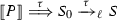satisfies the property for m steps (i.e., $\llbracket P \rrbracket \xrightarrow {\smash {\,\tau \,}}_{\ell } ^{m-1} S_0 \xrightarrow {\smash {\,\tau \,}}_{\ell } S$). We must prove for $k = m+1$:

  $$\begin{aligned} \llbracket P \rrbracket \xrightarrow {\smash {\,\tau \,}}_{\ell } ^{m} S \xrightarrow {\smash {\,\tau \,}}_{\ell } S' \end{aligned}$$

  by Lemma 9:

  $$\begin{aligned} S \equiv C_{\widetilde{x}\widetilde{y}}[ U_1 \parallel \dots \parallel U_n \parallel J ] \end{aligned}$$

  for some junk J and for all $i \in \{1, \ldots , n\}$ either:

  • 1. $U_i = \llbracket R_k \rrbracket$, where $R_k$ is a conditional redex reachable from P;

  • 2. $U_i = \llbracket R_k \rrbracket$, where $R_k$ is a pre-redex reachable from P;

  • 3. $U_i \in \{\![ R_k \mathord {\;|\;}R_j ]\!\}$, where redex $R_k \mathord {\;|\;}R_j$ is reachable from P.

  Then, by Lemma 10(a), there exists $\llbracket R_j \rrbracket$ such that:

  $$\begin{aligned} S&\equiv C_{\widetilde{x}\widetilde{y}}[ U_j \parallel \prod \limits _{i\in \{1\dots n\} \setminus j} U_i \parallel J ]\\ S'&\equiv C_{\widetilde{x}\widetilde{y}}[ U'_j \parallel \prod \limits _{i\in \{1\dots n\} \setminus j} U_i \parallel J' ] \end{aligned}$$

  and only cases (1) and (3) are considered:

  • Case $U_j = \llbracket R_j \rrbracket {}$ with $R_j$ a conditional redex: Since $\mathcal {I}_{S} \subseteq \mathcal {I}_{S'}$, by inspection on Fig. 8, we have $R_j = b?\,P_1\!:\!P_2$, with $b\in \{\texttt {tt} ,\texttt {ff} \}$ and the thesis follows as in the base case.

  • Case $U_j \in \{\![ R_j \mathord {\;|\;}R_{k} ]\!\}$: By inspection on Definition 30, combined with Corollary 2, $U_j \in \{\![ x \triangleleft l_j.Q \mathord {\;|\;}y \triangleright \{l_i:Q_i\}_{i\in I} ]\!\}$, for some Q, $Q_i$, $l_j$, and either

    (i) $U_j \cong ^{\pi }_\ell \overline{\mathsf {bra} (y,l_j)} \parallel \mathbf {\forall }{z}(\mathsf {bra} (z,l_j)\otimes \{z{:}x\} \rightarrow \llbracket Q \rrbracket ) \parallel \mathbf {\forall }{\epsilon }(l_j=l_j \rightarrow \llbracket Q_j \rrbracket {})$, or

    (ii) $U_j \cong ^{\pi }_\ell \llbracket Q \rrbracket \parallel \mathbf {\forall }{\epsilon }(l_j=l_j \rightarrow \llbracket Q_j \rrbracket {})$.

    We analyze each case:

    • Case (i): If $U_j = \overline{\mathsf {bra} (y,l_j)} \parallel \mathbf {\forall }{z}(\mathsf {bra} (z,l_j)\otimes \{z{:}x\} \rightarrow \llbracket Q \rrbracket ) \parallel \mathbf {\forall }{\epsilon }(l_j=l_j \rightarrow \llbracket Q_j \rrbracket )$ then, by Corollary 3, there exists $S_0$ such that:

      $$\begin{aligned} S_0 \equiv C_{\widetilde{x}\widetilde{y}}[ \overline{\{x{:}y\}} \parallel \llbracket x \triangleleft l_j.Q \mathord {\;|\;}y \triangleright \{l_i\,Q_i\}_{i\in I} \rrbracket {} \parallel U_1 \parallel \dots \parallel U_n \parallel J ] \end{aligned}$$

      by the semantics in Fig. 6 and Corollary 2:

      $$\begin{aligned} S_0&\xrightarrow {\smash {\,\tau \,}}_{\ell } C_{\widetilde{x}\widetilde{y}}[ \overline{\{x{:}y\}} \parallel U_j \parallel U_1 \parallel \dots \parallel U_n \parallel J ] = S \\&\xrightarrow {\smash {\,\tau \,}}_{\ell } C_{\widetilde{x}\widetilde{y}}[ \overline{\{x{:}y\}} \parallel \overline{\mathsf {bra} (y,l_j)} \parallel \mathbf {\forall }{z}(\mathsf {bra} (z,l_j)\otimes \{z{:}x\} \rightarrow \llbracket Q \rrbracket ) \parallel \llbracket Q_j \rrbracket {} \\&\qquad \qquad \quad \parallel U_1 \parallel \dots \parallel U_n \parallel J \parallel ] = S'\\&\xrightarrow {\smash {\,\tau \,}}_{\ell } \cong ^{\pi }_\ell C_{\widetilde{x}\widetilde{y}}[ \\ ]&{\overline{\{x{:}y\}} \parallel \llbracket Q \rrbracket {} \parallel \llbracket Q_j \rrbracket {} \parallel U_1 \parallel \dots \parallel U_n \parallel J \parallel \prod \limits _{h\in I}\mathbf {\forall }{\epsilon }(l_h = l_j \rightarrow \llbracket Q_i \rrbracket ) } \end{aligned}$$

      The proof finalizes by letting $J' = J \parallel \prod \limits _{h\in I}\mathbf {\forall }{\epsilon }(l_h = l_j \rightarrow \llbracket Q_i \rrbracket )$.

    • Case (ii): If $U_j = \llbracket Q \rrbracket \parallel \mathbf {\forall }{\epsilon }(l_j=l_j \rightarrow \llbracket Q_j \rrbracket {})$ then, by Definition 30 and Notation 14, there exists $S_0$ such that:

      

      by the semantics in Fig. 6:

      $$\begin{aligned} S_0&\xrightarrow {\smash {\,\tau \,}}_{\ell } C_{\widetilde{x}\widetilde{y}}[ \overline{\{x{:}y\}} \parallel \overline{\mathsf {bra} (y,l_j)} \parallel \mathbf {\forall }{z}(\mathsf {bra} (z,l_j)\otimes \{z{:}x\} \rightarrow \llbracket Q \rrbracket ) \parallel \llbracket Q_j \rrbracket {} \\&\qquad \qquad \quad \parallel U_1 \parallel \dots \parallel U_n \parallel J ] = S\\&\xrightarrow {\smash {\,\tau \,}}_{\ell } C_{\widetilde{x}\widetilde{y}}[ \overline{\{x{:}y\}}\\&\parallel \llbracket Q \rrbracket \parallel \llbracket Q_j \rrbracket \parallel U_1 \parallel \dots \parallel U_n \parallel J \parallel \prod \limits _{h\in I}\mathbf {\forall }{\epsilon }(l_h = l_j \rightarrow \llbracket Q_i \rrbracket ) ] = S' \end{aligned}$$

      The proof finishes by letting $J' = J \parallel \prod \limits _{h\in I} \mathbf {\forall }{\epsilon }(l_h = l_j \rightarrow \llbracket Q_i \rrbracket )$.

$\square$

Proposition 1

Suppose S is a target term (cf. Definition 26).

• 1. $S \equiv C_{\widetilde{x}\widetilde{y}}[ \overline{c_1} \parallel \dots \parallel \overline{c_n} \parallel Q_1 \parallel \dots \parallel Q_k ]$ with $n, k\ge 1$, where every $c_j = \gamma _j(x_j,m_j)$ (with $1\le j \le n$), for some value or label $m_j$, and every $Q_i$ (with $1\le i \le k$) is an abstraction (possibly replicated).

• 2. For every $i,j\in \{1,\dots ,n\}$, $i\not = j$ implies $c_i = \gamma _i(x_i,m_i)$, $c_j = \gamma _j(x_j,m_j)$, and $x_i\not = x_j$.

Proof

The first part of the statement follows immediately from the definition of $\llbracket \cdot \rrbracket$ (cf. Definition 25), Lemma 9, and by applying the structural congruence of $\texttt {lcc}$ in S.

The second part of the statement is proven by contradiction. We assume that $S \equiv C_{\widetilde{x}\widetilde{y}}[ \overline{c_1} \parallel \dots \parallel \overline{c_n} \parallel Q ]$, where $Q = Q_1 \parallel \dots \parallel Q_k$ where every $Q_r$, $r\in \{1,\dots ,k\}$ is an abstraction (possibly replicated) and that there exist $i,j\in \{1,\dots ,n\}$ such that $i\not = j$, $c_i = \gamma (x_1,m_1)$, $c_j = \gamma (x_2,m_2)$, and $x_1 = x_2$. We proceed by a case analysis on $\gamma$; there are four cases, we only show the cases $\gamma = \mathsf {snd}$ and $\gamma = \mathsf {rcv}$.

• 1. Suppose that $\gamma = \mathsf {snd}$. By assumption,

  $$\begin{aligned} S \equiv C_{\widetilde{x}\widetilde{y}}[ \overline{c_1} \parallel \dots \parallel \overline{\mathsf {snd} (x, v_1)} \parallel \dots \parallel \overline{\mathsf {snd} (x, v_2)} \parallel \dots \parallel \overline{c_n} \parallel Q ] \end{aligned}$$

  Moreover, by Definition 26, S must come from the translation of a well-typed term. By Fig. 8, it must be the case that:

  $$\begin{aligned} S \equiv C_{\widetilde{x}\widetilde{y}}[ \overline{c_1} \parallel \dots \parallel \llbracket {x}\langle v_1\rangle .P_1 \rrbracket \parallel \dots \parallel \llbracket {x}\langle v_2\rangle .P_2 \rrbracket \parallel \dots \parallel \overline{c_n} \parallel Q' ] \end{aligned}$$

  for some $Q'$ that does not contain the abstractions used to build the translations $\llbracket {x}\langle v_k\rangle .P_k \rrbracket$, $k\in \{1,2\}$. This implies, by Fig. 8, that S comes from a $\pi$ process that contains two outputs on the same channel x in parallel. This contradicts the well-formedness assumption that follows from Theorem 4, finishing the proof.

• 2. Suppose that $\gamma = \mathsf {rcv}$. The proof has the same structure as the one above. The only difference is that rather than the translation of output processes, we must consider intermediate redexes (cf. Fig. 11). Similarly as above, we will find that the well-formedness assumption induced by typing is violated, thus reaching a contradiction.

$\square$

Lemma 12

(Invariants of Target Terms (II): Consuming Information) Let P be a well-typed $\pi$ program. For any $S, S'$ such that and $\mathcal {I}_{S} \not \subseteq \mathcal {I}_{S'}$ the following holds, for some U:

• (1) If $\mathcal {I}_{S} \setminus \mathcal {I}_{S'} = \{\mathsf {snd} (x_1,v)\}$, then all the following hold:

  • (a) $S \equiv C_{\widetilde{x}\widetilde{y}}[ \overline{\{x_1{:}y_1\}} \parallel \llbracket {x_1}\langle v\rangle .P_1 \mathord {\;|\;}\diamond y_1(z).P_2 \rrbracket \parallel U ]$;

  • (b) ;

  • (c) , where $S'' = \mathbf {*}\, \llbracket y(z).P_2 \rrbracket$ or $S'' = \overline{\texttt {tt}}$.

• (2) If $\mathcal {I}_{S} \setminus \mathcal {I}_{S'} = \{\mathsf {rcv} (x_1,v)\}$, then there exists $S_0$ such that and all of the following hold:

  • (a) $S_0 \equiv C_{\widetilde{x}\widetilde{y}}[ \overline{\{x_1{:}y_1\}} \parallel \llbracket {y_1}\langle v\rangle .P_1 \mathord {\;|\;}\diamond ~x_1(z).P_2 \rrbracket \parallel U ]$;

  • (b) ;

  • (c) , where $S'_1 = \mathbf {*}\, \llbracket y(z).P_2 \rrbracket$ or $S'_1 = \overline{\texttt {tt}}$.

• (3) If $\mathcal {I}_{S} \setminus \mathcal {I}_{S'} = \{\mathsf {sel} (x_1,l_j)\}$, then all of the following hold:

  • (a) $S \equiv C_{\widetilde{x}\widetilde{y}}[ \overline{\{x_1{:}y_1\}} \parallel \llbracket x_1 \triangleleft l.P_1 \mathord {\;|\;}y_1 \triangleright \{l_i:P_i\}_{i\in I} \rrbracket U ]$;

  • (b) ;

  • (c) $S_1 \xrightarrow {\smash {\,\tau \,}}_{\ell } ^{2} \cong ^{\pi }_\ell C_{\widetilde{x}\widetilde{y}}[ \llbracket P_1 \mathord {\;|\;}P_j \rrbracket \parallel U' ]$, with $U' \equiv U \parallel \prod _{h\in I}\mathbf {\forall }{\epsilon }(l_h = l_j \rightarrow \llbracket Q_h \rrbracket )$.

• (4) If $\mathcal {I}_{S} \setminus \mathcal {I}_{S'} = \{\mathsf {bra} (x,l_j)\}$, then there exists

  $S_0 \equiv C_{\widetilde{x}\widetilde{y}}[ \overline{\{x{:}y\}} \parallel \llbracket y \triangleleft l_j.Q \mathord {\;|\;}x \triangleright \{l_i\,Q_i\}_{i\in I} \rrbracket \parallel U ]$ such that and either:

  • (a) All of the following hold:

    • (i) ,

    • (ii) (and)

    • (iii) $S' = C_{\widetilde{x}\widetilde{y}}[ \overline{\{x{:}y\}}\parallel \llbracket Q\mathord {\;|\;}Q_j \rrbracket \parallel U' ]$.

  • (b) All of the following hold:

    • (i) ,

    • (ii) (and)

    • (iii) $S' \xrightarrow {\smash {\,\tau \,}}_{\ell } C_{\widetilde{x}\widetilde{y}}[ \overline{\{x{:}y\}}\parallel \llbracket P \mathord {\;|\;}Q_j \rrbracket \parallel U' ]$.

  with $U' \equiv U \parallel \prod _{h\in I}\mathbf {\forall }{\epsilon }(l_h = l_j \rightarrow \llbracket Q_h \rrbracket )$.

Proof

By induction on the transition . By Lemma 1:

$$\begin{aligned} \llbracket P \rrbracket \equiv \exists \widetilde{x},\widetilde{y}.(\llbracket R_1 \rrbracket \parallel \dots \parallel \,\llbracket R_n \rrbracket \parallel !\overline{\bigotimes \limits _{\begin{array}{c} x_i\in \widetilde{x},\\ \!\! y_i\in \widetilde{y} \end{array} }\{x_i{:}y_i\} } ) \end{aligned}$$

(1)

where each $R_i$ is a pre-redex or a conditional process. Also, by Lemma 10(b), the difference of observables between a process and the process obtained in a single $\tau$-transition is a singleton. Therefore, we apply a case analysis on each one of those singletons.

• Base Case: Then, . Let $\llbracket P \rrbracket = S$. By assumption, $S \xrightarrow {\smash {\,\tau \,}}_{\ell } S'$ and $\mathcal {I}_{S} \not \subseteq \mathcal {I}_{S'}$. Thus, there is a $c\in \mathcal {I}_{S}$ such that $c\not \in \mathcal {I}_{S'}$. Considering Eq. (1) and by inspection on Fig. 8 we only analyze from Case (2), as cases (1) and (3) do not apply: Case (1) does not apply as it does not entail constraint consumption (cf. Lemma 10(a)) and Case (3) does not apply as there are no intermediate redexes in S.

  • Case $\mathcal {I}_{S} \setminus \mathcal {I}_{S'} = \{\mathsf {snd} (x_1,v)\}$: By Lemma 6, there exists j such that:

    $$\begin{aligned} S \equiv C_{\widetilde{x}\widetilde{y}}[ \llbracket R_j \rrbracket \parallel \prod \limits _{i\in \{1\dots n\} \setminus j} \llbracket R_i \rrbracket {} ] \end{aligned}$$

    where $\llbracket R_j \rrbracket {} \equiv \llbracket {x_j}\langle v\rangle .Q \rrbracket {}$. Since $\mathcal {I}_{S} \not \subseteq \mathcal {I}_{S'}$, and every $c\in \mathcal {I}_{S}$ is unique, by inspection on Fig. 8 and Lemma 7, there must exist an $R_k$ such that:

    $$\begin{aligned} S \equiv C_{\widetilde{x}\widetilde{y}}[ \llbracket {x_j}\langle v\rangle .Q \rrbracket \parallel \llbracket R_k \rrbracket {} \parallel \prod \limits _{i\in \{1\dots n\} \setminus \{j,k\}} \llbracket R_i \rrbracket {} ] \end{aligned}$$

    where $\llbracket R_k \rrbracket {} \equiv \llbracket y_j(z).Q' \rrbracket$ or $\llbracket R_k \rrbracket {} \equiv \llbracket \mathbf {*}\, y_j(z).Q' \rrbracket$. Without loss of generality, we only show the case for $\llbracket R_k \rrbracket {} \equiv \llbracket y_j(z).Q' \rrbracket$:

    $$\begin{aligned} S \equiv C_{\widetilde{x}\widetilde{y}}[ \llbracket {x_j}\langle v\rangle .Q \rrbracket \parallel \llbracket y_j(z).Q' \rrbracket {} \parallel \prod \limits _{i\in \{1\dots n\} \setminus \{j,k\}} \llbracket R_i \rrbracket {} ] \end{aligned}$$

    By the semantics of $\texttt {lcc}$ (cf. Fig. 6) and Lemma 8:

    

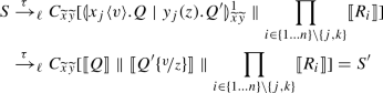
  • Case $\mathcal {I}_{S} \setminus \mathcal {I}_{S'} = \{\mathsf {sel} (x_1,l_j)\}$: By Lemma 6, there exists j such that:

    $$\begin{aligned} S \equiv C_{\widetilde{x}\widetilde{y}}[ \llbracket R_j \rrbracket \parallel \prod \limits _{i\in \{1\dots n\} \setminus j} \llbracket R_i \rrbracket {} ] \end{aligned}$$

    where $\llbracket R_j \rrbracket {} \equiv \llbracket x_j \triangleleft l_j.Q \rrbracket {}$. Furthermore, by following the same analysis as in the previous case, there must exist $R_j$, such that:

    $$\begin{aligned} S \equiv C_{\widetilde{x}\widetilde{y}}[ \llbracket x_j \triangleleft l_j.Q \rrbracket \parallel \llbracket R_k \rrbracket {} \parallel \prod \limits _{i\in \{1\dots n\} \setminus \{j,k\}} \llbracket R_i \rrbracket {} ] \end{aligned}$$

    where $\llbracket R_k \rrbracket {} \equiv \llbracket y_j \triangleright \{l_i: Q_i\}_{i\in I} \rrbracket$. Then, by the semantics of $\texttt {lcc}$ (cf. Fig. 6):

    

• Inductive Case: By IH, satisfies the property for m steps (i.e., $\llbracket P \rrbracket \xrightarrow {\smash {\,\tau \,}}_{\ell } ^{m-1} S \xrightarrow {\smash {\,\tau \,}}_{\ell } S'$). Therefore:

  $$\begin{aligned} S \equiv C_{\widetilde{x}\widetilde{y}}[ U_1 \parallel \dots \parallel U_n \parallel J ] \end{aligned}$$

  for some junk J and for all $i \in \{1, \ldots , n\}$ either:

  • 1. $U_i = \llbracket R_k \rrbracket$, where $R_k$ is a conditional redex reachable from P;

  • 2. $U_i = \llbracket R_k \rrbracket$, where $R_k$ is a pre-redex reachable from P;

  • 3. $U_i \in \{\![ R_k \mathord {\;|\;}R_j ]\!\}$, where redex $R_k \mathord {\;|\;}R_j$ is reachable from P.

  We now have to prove for $k = m+1$:

  $$\begin{aligned} \llbracket P \rrbracket \xrightarrow {\smash {\,\tau \,}}_{\ell } ^{k} S \xrightarrow {\smash {\,\tau \,}}_{\ell } S' \end{aligned}$$

  Since $S \xrightarrow {\smash {\,\tau \,}}_{\ell } S'$, there exists $\llbracket R_j \rrbracket$ such that:

  $$\begin{aligned} S&\equiv C_{\widetilde{x}\widetilde{y}}[ U_j \parallel \prod \limits _{i\in \{1\dots n\} \setminus j} U_i \parallel J ]\\ S'&\equiv C_{\widetilde{x}\widetilde{y}}[ U'_j \parallel \prod \limits _{i\in \{1\dots n\} \setminus j} U_i \parallel J' ] \end{aligned}$$

  As above, we distinguish only cases for (2), (3). Notice that using Lemma 10(a) and Lemma 11 we can discard case (1):

  • Case (2): Proceeds as the base case, by distinguishing cases between the consumed constraints. The cases correspond to constraints $\mathsf {snd} ,\mathsf {sel}$ (cf. Fig. 7).

  • Case (3): By inspection on Definition 30 and Notation 14, we distinguish two cases corresponding to predicates $\mathsf {rcv} ,\mathsf {bra}$ (cf. Fig. 7):

    • Case $\mathcal {I}_{S} \setminus \mathcal {I}_{S'} = \{\mathsf {rcv} (x_1,v)\}$: By Lemmas 6 and 7, there exists j such that:

      $$\begin{aligned} S \equiv C_{\widetilde{x}\widetilde{y}}[ U_j \parallel U_1 \parallel \dots \parallel U_n \parallel J ] \end{aligned}$$

      where $U_j = \overline{\mathsf {rcv} (x_j,v)} \parallel W$, for some W. By inspection on Definition 30 and Lemma 7, there exists $U_k$ such that $U_j \parallel U_k \in \{\![ x_j(z).Q \mathord {\;|\;}{y_j}\langle v\rangle .Q' ]\!\}$ or $U_j \parallel U_k \!\in \! \{\![ \mathbf {*}\, x_j(z).Q \mathord {\;|\;}{y_j}\langle v\rangle .Q' ]\!\}$, for some $x_j,y_j,v$. Without loss of generality, we will only analyze the case when $U_j \parallel U_k \!\in \!\{\![ x_j(z).Q \mathord {\;|\;}{y_j}\langle v\rangle .Q' ]\!\}$. By Definition 30 and Notation 14, . By expanding the previous definitions:

      

      and by the application of Rule ${(\textsc {C:Sync})}$ in Fig. 6 (i.e., the $\texttt {lcc}$ semantics):

      

    • Case $\mathcal {I}_{S} \setminus \mathcal {I}_{S'} = \{\mathsf {bra} (x,l_j)\}$: This case proceeds as above. The conclusion is reached using the same analysis as in the inductive case in the proof of Lemma 11.

$\square$

1.5 A diamond property for target terms

Lemma 13

Let S be a target term (cf. Definition 26) and x, y be endpoints. Then, $S \xrightarrow {\smash {\,\tau \,}}_{\ell } S'$ if and only if $S \xrightarrow {\,{\eta }\,}_{\ell } S'$ where ${\eta } \in \{\alpha (x,y) \, {\mid }\,\alpha \!\in \!\{\texttt {IO},\texttt {SL}, \texttt {RP}, \texttt {IO}_1, \texttt {RP}_1, \texttt {SL}_1, \texttt {SL}_2, \texttt {SL}_3\} \wedge x,y\in \mathcal {V}_{\pi } \}\cup \{\texttt {CD}(-)\}$.

Proof

We prove both directions:

• $\Rightarrow$) By Corollary 4, $S = C_{\widetilde{x}\widetilde{y}}[ U_1 \parallel \dots \parallel U_n ]$, with $U_i = \llbracket R_i \rrbracket$ for some pre-redex $R_i$ (cf. Definition 9). We take then an arbitrary $U_i$, $i\in \{1,\dots , n\}$. We apply a case analysis on $U_i$. There are 11 cases corresponding to each possible shape of $U_i$. We only show three cases; the rest are similar:

  • Case $U_i = \llbracket {x}\langle v\rangle .P_1 \rrbracket$: We distinguish two sub-cases, depending on whether there exists $U_j$ such that $U_j = \llbracket y(z).P_2 \rrbracket$ and $x\in \widetilde{x},y\in \widetilde{y}$ or not. The latter case is vacuously true, as there would not be any transition to check. We show the former case:

    • Sub-case $\exists U_j.(U_j = \llbracket y(z).P_2 \rrbracket \wedge x\in \widetilde{x},y\in \widetilde{y})$:

      • 1. $S \equiv C_{\widetilde{x}\widetilde{y}}[ \llbracket {x}\langle v\rangle .P_1 \rrbracket \parallel \llbracket y(z).P_2 \rrbracket \parallel U_1 \parallel \dots \parallel U_n ]$    (Assumption).

      • 2.    (Rule ${(\textsc {C:Sync})}$ - Fig. 6, (1), Assumption).

      • 3. $S \xrightarrow {\,{\texttt {IO}_1(x,y)}\,}_{\ell } S'$    (Definition 31, (1), (2)).

  • Case $U_i = \llbracket x(y).P_1 \rrbracket$: Symmetric to the previous case, as $U_j = \llbracket {y}\langle v\rangle .P_2 \rrbracket$.

  • Case :

    • 1.    (Assumption).

    • 2.    (Rule ${(\textsc {C:Sync})}$ - Fig. 6, (1), Assumption).

    • 3. $S \xrightarrow {\,{\texttt {IO}_1(x,y)}\,}_{\ell } S'$    (Definition 31, (1), (2)).

• $\Leftarrow$) This direction proceeds by applying a case analysis on label $\eta$. Each case then will proceed by applying Rule ${(\textsc {C:Sync})}$ in Fig. 6 and showing that the transition yields the correct process.

$\square$

Lemma 14

Let S be a target term such that $S\xrightarrow {\smash {\,\omega \,}}_{\ell } S_1$ and , where ${\gamma (\widetilde{x}\widetilde{y})}$ is a closing sequence (cf. Notation 16). Then, there exists $S_3$ such that and $S_2 \xrightarrow {\smash {\, \omega \,}}_{\ell } S_3$.

Proof

By induction on the length n of $|{\gamma (\widetilde{x}\widetilde{y})}|$.

• Base Case: $n = 0$. Then:

  • 1. $S \xrightarrow {\smash {\,\omega \,}}_{\ell } S_1$    (Assumption).

  • 2.    (Assumption)

  • 3.    (Fig. 6)

  Conclude by letting $S_1 = S_1$, $S_2 = S$ and $S_3 = S_1$ and using (1),(3).

• Inductive Step: $n\ge 1$. We state the IH:

  • IH: If $S\xrightarrow {\smash {\,\omega \,}}_{\ell } S_1$ and , then there exists $S'_0$ such that and $S_0 \xrightarrow {\smash {\,\omega \,}}_{\ell } S'_0$.

  We distinguish cases for $\kappa \in \{\texttt {IO}_1, \texttt {RP}_1, \texttt {CD}, \texttt {SL}_2, \texttt {SL}_3\}$. There are five cases and each one has four sub-cases, corresponding to the opening labels $\{\texttt {IO},\texttt {SL}, \texttt {RP}, \texttt {SL}_1\}$.

  We detail three cases: $\kappa = \texttt {IO}_1$, $\kappa = \texttt {RP}_1$ and $\kappa = \texttt {CD}$, as the other are similar:

  • Case $\kappa = \texttt {IO}_1$: As mentioned above, there are four sub-cases depending on $\omega$. We enumerate them below and only detail $\omega = \texttt {IO}$, $\omega = \texttt {RP}$:

    • Sub-case $\omega =\texttt {IO}$: Suppose, without loss of generality, that the actions take place on endpoints x, y and w, z. Furthermore, by typing and Corollary 1 and Definition 10, it cannot be the case that $x = w$ and $y = z$, because this would imply that there are more than one output prefixed on x. Then, we we only consider the case when $x \not = w$ and $y\not = z$:

      • Sub-case $x \not = w \wedge y \not = z$: We proceed as follows:

        • 1. $S = C_{\widetilde{x}\widetilde{y}}[ U_1 \parallel \dots \parallel \llbracket {x}\langle v\rangle .Q_1 \rrbracket \parallel \llbracket y(u_1).Q_2 \rrbracket \parallel \dots \parallel U_n\parallel J ]$    (Assumption, Fig. 13, Lemma 9).

        • 2.    (Fig. 6,(1)).

        • 3. , $m\ge 1$    (IH, (1), Lemma 9).

        • 4.    ((3), Fig. 6).

        • 5. $S_0 \xrightarrow {\smash {\,\texttt {IO}(x,y)\,}}_{\ell } S'_0$    (IH)

        • 6.    (Fig. 6, (5)).

        • 7.    (IH).

        We can then reduce the proof to the existence of some $S_3$ such that

        –:

        $S_2 \xrightarrow {\smash {\,\texttt {IO}(x,y)\,}}_{\ell } S_3$ and

        –:

        $S'_0\xrightarrow {\smash {\,\texttt {IO}_1(w,z)\,}}_{\ell } S_3$

        We have:

        • (a) .

        • (b) .

        then, let

        

        and we can show by Fig. 6 that $S'_0\xrightarrow {\smash {\,\texttt {IO}_1(w,z)\,}}_{\ell } S_3$ and $S_2 \xrightarrow {\smash {\,\texttt {IO}(x,y)\,}}_{\ell } S_3$, which concludes the proof.

    • Sub-case $\omega = \texttt {RP}$: As above, assume the actions take place in variables x, y and w, z. It is not possible for them to happen in the same variable, by Corollary 1.

      • 1. $S = C_{\widetilde{x}\widetilde{y}}[ U_1 \parallel \dots \parallel \llbracket {x}\langle v\rangle .Q_1 \rrbracket \parallel \llbracket \mathbf {*}\, y(u_1).Q_2 \rrbracket \parallel \dots \parallel U_n\parallel J ]$    (Assumption, Fig. 13, Lemma 9).

      • 2.    (Fig. 6,(1)).

      • 3. , $m\ge 1$    (IH, (1), Lemma 9).

      • 4.    ((3), Fig. 6).

      • 5. $S_0 \xrightarrow {\smash {\,\texttt {RP}(x,y)\,}}_{\ell } S'_0$    (IH)

      • 6.    (Fig. 6, (5)).

      • 7.    (IH).

      We reduce the proof to show to the existence of some $S_3$ such that

      • $S_2 \xrightarrow {\smash {\,\texttt {RP}(x,y)\,}}_{\ell } S_3$ and

      • $S'_0\xrightarrow {\smash {\,\texttt {IO}_1(w,z)\,}}_{\ell } S_3$

      We have:

      • (a) .

      • (b) .

      Then, let

      

      and we can show by Fig. 6 that $S'_0\xrightarrow {\smash {\,\texttt {IO}_1(w,z)\,}}_{\ell } S_3$ and $S_2 \xrightarrow {\smash {\,\texttt {RP}(x,y)\,}}_{\ell } S_3$, which concludes the proof.

    • Sub-case $\omega = \texttt {SL}($): Similarly as above.

    • Sub-case $\omega = \texttt {SL}_1($): Similarly as above.

  • Case $\kappa = \texttt {RP}_1$: We proceed similarly as above. The most interesting case is whenever $\omega = \texttt {RP}$:

    • Sub-case $\omega = \texttt {RP}$: As above, assume the actions take place in variables x, y and w, z. It is not possible for them to happen in the same variable, by Corollary 1.

      • 1. $S = C_{\widetilde{x}\widetilde{y}}[ U_1 \parallel \dots \parallel \llbracket {x}\langle v\rangle .Q_1 \rrbracket \parallel \llbracket \mathbf {*}\, y(u_1).Q_2 \rrbracket \parallel \dots \parallel U_n\parallel J ]$    (Assumption, Fig. 13, Lemma 9).

      • 2.    (Fig. 6,(1)).

      • 3. , $m\ge 1$    (IH, (1), Lemma 9).

      • 4.    ((3), Fig. 6).

      • 5. $S_0 \xrightarrow {\smash {\,\texttt {RP}(x,y)\,}}_{\ell } S'_0$    (IH)

      • 6.    (Fig. 6, (5)).

      • 7.    (IH).

      We reduce the proof to show that there exists some $S_3$ such that

      • $S_2 \xrightarrow {\smash {\,\texttt {RP}(x,y)\,}}_{\ell } S_3$ and

      • $S'_0\xrightarrow {\smash {\,\texttt {RP}_1(w,z)\,}}_{\ell } S_3$

      We have:

      • (a)
      • (b)

      Then, let

      

      and we can show by Fig. 6 that $S'_0\xrightarrow {\smash {\,\texttt {RP}_1(w,z)\,}}_{\ell } S_3$ and $S_2 \xrightarrow {\smash {\,\texttt {RP}(x,y)\,}}_{\ell } S_3$, which concludes the proof.

    • Sub-case $\omega = \texttt {IO}$: Similarly as above.

    • Sub-case $\omega = \texttt {SL}$: Similarly as above.

    • Sub-case $\omega = \texttt {SL}_1$: Similarly as above.

  • Case $\kappa = \texttt {CD}$: As above we distinguish four cases. We only show sub-case $\omega = \texttt {IO}$, as the other cases are similar:

    • Sub-case $\omega = \texttt {IO}$: Assume that the $\texttt {IO}$ transition happens on endpoints x, y. Since $\texttt {CD}$ does not occur on any channels, we do not need to assume more endpoints:

      • 1. $S = C_{\widetilde{x}\widetilde{y}}[ U_1 \parallel \dots \parallel \llbracket {x}\langle v\rangle .Q_1 \rrbracket \parallel \llbracket y(z).Q_2 \rrbracket \parallel \dots \parallel U_n ]$, $n\ge 1$    (Assumption, Fig. 13, Lemma 9 ).

      • 2. , $n\ge 1$    ((1), Fig. 13).

      • 3. $S_0 = C_{\widetilde{x}\widetilde{y}}[ U'_1 \parallel \dots \parallel \llbracket {x}\langle v\rangle .Q_1 \rrbracket \parallel \llbracket y(z).Q_2 \rrbracket \parallel \llbracket b?\,Q_3\!:\!Q_4 \rrbracket \parallel \dots \parallel U'_m ]$, $m\ge 1$, with $b\in \{\texttt {tt},\texttt {ff}\}$    (IH, Fig. 13).

      • 4. $S_2 = C_{\widetilde{x}\widetilde{y}}[ U'_1 \parallel \dots \parallel \llbracket {x}\langle v\rangle .Q_1 \rrbracket \parallel \llbracket y(z).Q_2 \rrbracket \parallel \llbracket Q_i \rrbracket \parallel \dots \parallel U'_m ]$, $i\in \{3,4\}$    ((3), Fig. 13 ).

      • 5. , $m\ge 1$, with $b\in \{\texttt {tt},\texttt {ff}\}$    (IH, Fig. 13).

      Now, let , $m\ge 1$, with $b\in \{\texttt {tt},\texttt {ff}\}$, $i\in \{3,4\}$.

      It can be shown, by Fig. 13 that $S_2 \xrightarrow {\smash {\,\texttt {IO}(x,y)\,}}_{\ell } S_3$ and $S'_0 \xrightarrow {\smash {\,\texttt {CD}(-)\,}}_{\ell } S_3$ which by IH imply that , concluding the proof.

    • Sub-case $\omega = \texttt {RP}$: Similarly as above.

    • Sub-case $\omega = \texttt {SL}$: Similarly as above.

    • Sub-case $\omega = \texttt {SL}_1$: Similarly as above.

  • Case $\kappa = \texttt {SL}_2$: Similarly as Case $\omega = \texttt {IO}_1$.

  • Case $\kappa = \texttt {SL}_3$: Similarly as Case $\omega = \texttt {IO}_1$.

$\square$

Lemma 15

Suppose a well-typed $\pi$ program P. For every sequence of labels ${\gamma (\widetilde{x}\widetilde{y})}$ such that , there exist Q, $S'$, and $\gamma '(\widetilde{x}\widetilde{y})$ such that $P\longrightarrow ^*Q$ and , with $\gamma '(\widetilde{x}\widetilde{y}) = {\gamma (\widetilde{x}\widetilde{y})}\!\!\downarrow$ (cf. Definition 35). Moreover, $\llbracket Q \rrbracket \cong ^{\pi }_\ell S'$.

Proof

By induction on $|{\gamma (\widetilde{x}\widetilde{y})}|$ and a case analysis on the last label of the sequence. The base case is immediate since and $P\longrightarrow ^* P$.

For the inductive step, assume $|{\gamma (\widetilde{x}\widetilde{y})}| = n\ge 0$. We state the IH:

• IH: if , then there exists $Q_0,S'_0$ and $\gamma '_0(\widetilde{x}\widetilde{y})$ such that $P \longrightarrow ^* Q$, , $\gamma '_0(\widetilde{x}\widetilde{y}) = {\gamma (\widetilde{x}\widetilde{y})}\!\!\downarrow$ and $S'_0\cong ^{\pi }_\ell \llbracket Q \rrbracket$.

Using the IH, the proof can be summarized by the diagram in Fig. 14, where we must show the existence of the dotted arrows. Details follow:

• Base Case: $n = 0$. Then:

  • 1. $S \xrightarrow {\smash {\,\omega \,}}_{\ell } S_1$    (Assumption).

  • 2.    (Assumption)

  • 3.    (Fig. 6)

  Conclude by letting $S_1 = S_1$, $S_2 = S$ and $S_3 = S_1$ and using (1),(3).

• Inductive Step: $n\ge 1$. We state the IH:

  • IH: If $S\xrightarrow {\smash {\,\omega \,}}_{\ell } S_1$ and 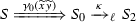, then there exists $S'_0$ such that and $S_0 \xrightarrow {\smash {\,\omega \,}}_{\ell } S'_0$.

  We distinguish cases for $\kappa \in \{\texttt {IO}_1, \texttt {RP}_1, \texttt {CD}, \texttt {SL}_2, \texttt {SL}_3\}$. There are five cases and each one has four sub-cases, corresponding to the opening labels $\{\texttt {IO},\texttt {SL}, \texttt {RP}, \texttt {SL}_1\}$. We detail three cases: $\kappa = \texttt {IO}_1$, $\kappa = \texttt {RP}_1$ and $\kappa = \texttt {CD}$, as the other are similar:

  • Case $\kappa = \texttt {IO}_1$: As mentioned above, there are four sub-cases depending on $\omega$. We enumerate them below and only detail $\omega = \texttt {IO}$, $\omega = \texttt {RP}$:

    • Sub-case $\omega =\texttt {IO}$: Suppose, without loss of generality, that the actions take place on endpoints x, y and w, z. Furthermore, by typing and Corollary 1 and Definition 10, it cannot be the case that $x = w$ and $y = z$, because this would imply that there is more than one output prefixed on x. Then, we we only consider the case when $x \not = w$ and $y\not = z$:

      • Sub-case $x \not = w \wedge y \not = z$: We proceed as follows:

        • 1. $S = C_{\widetilde{x}\widetilde{y}}[ U_1 \parallel \dots \parallel \llbracket {x}\langle v\rangle .Q_1 \rrbracket \parallel \llbracket y(u_1).Q_2 \rrbracket \parallel \dots \parallel U_n\parallel J ]$    (Assumption, Fig. 13, Lemma 9).

        • 2.    (Fig. 6,(1)).

        • 3. , $m\ge 1$    (IH, (1), Lemma 9).

        • 4.    ((3), Fig. 6).

        • 5. $S_0 \xrightarrow {\smash {\,\texttt {IO}(x,y)\,}}_{\ell } S'_0$    (IH)

        • 6.    (Fig. 6, (5)).

        • 7.    (IH).

        We can then reduce the proof to the existence of some $S_3$ such that

        –:

        $S_2 \xrightarrow {\smash {\,\texttt {IO}(x,y)\,}}_{\ell } S_3$ and

        –:

        $S'_0\xrightarrow {\smash {\,\texttt {IO}_1(w,z)\,}}_{\ell } S_3$

        We have:

        • (a) .

        • (b) .

        Then, let

        

        and we can show by Fig. 6 that $S'_0\xrightarrow {\smash {\,\texttt {IO}_1(w,z)\,}}_{\ell } S_3$ and $S_2 \xrightarrow {\smash {\,\texttt {IO}(x,y)\,}}_{\ell } S_3$, which concludes the proof.

    • Sub-case $\omega = \texttt {RP}$: As above, assume the actions take place in variables x, y and w, z. It is not possible for them to happen in the same variable, by Corollary 1.

      • 1. $S = C_{\widetilde{x}\widetilde{y}}[ U_1 \parallel \dots \parallel \llbracket {x}\langle v\rangle .Q_1 \rrbracket \parallel \llbracket \mathbf {*}\, y(u_1).Q_2 \rrbracket \parallel \dots \parallel U_n\parallel J ]$    (Assumption, Fig. 13, Lemma 9).

      • 2.    (Fig. 6,(1)).

      • 3. , $m\ge 1$    (IH, (1), Lemma 9).

      • 4.    ((3), Fig. 6).

      • 5. $S_0 \xrightarrow {\smash {\,\texttt {RP}(x,y)\,}}_{\ell } S'_0$    (IH)

      • 6.    (Fig. 6, (5)).

      • 7.    (IH).

      We reduce the proof to the existence of some $S_3$ such that

      • $S_2 \xrightarrow {\smash {\,\texttt {RP}(x,y)\,}}_{\ell } S_3$

      • $S'_0\xrightarrow {\smash {\,\texttt {IO}_1(w,z)\,}}_{\ell } S_3$

      We have:

      • (a) .

      • (b) .

      Then, let

      

      and we can show by Fig. 6 that $S'_0\xrightarrow {\smash {\,\texttt {IO}_1(w,z)\,}}_{\ell } S_3$ and $S_2 \xrightarrow {\smash {\,\texttt {RP}(x,y)\,}}_{\ell } S_3$, which concludes the proof.

    • Sub-cases $\omega = \texttt {SL}$ and $\omega = \texttt {SL}_1$: Similarly as above.

  • Case $\kappa = \texttt {RP}_1$: We proceed similarly as above. The most interesting case is whenever $\omega = \texttt {RP}$:

    • Sub-case $\omega = \texttt {RP}$: As above, assume the actions take place in variables x, y and w, z. It is not possible for them to happen in the same variable, by Corollary 1.

      • 1. $S = C_{\widetilde{x}\widetilde{y}}[ U_1 \parallel \dots \parallel \llbracket {x}\langle v\rangle .Q_1 \rrbracket \parallel \llbracket \mathbf {*}\, y(u_1).Q_2 \rrbracket \parallel \dots \parallel U_n\parallel J ]$    (Assumption, Fig. 13, Lemma 9).

      • 2.    (Fig. 6,(1)).

      • 3. , $m\ge 1$    (IH, (1), Lemma 9).

      • 4.    ((3), Fig. 6).

      • 5. $S_0 \xrightarrow {\smash {\,\texttt {RP}(x,y)\,}}_{\ell } S'_0$    (IH)

      • 6.    (Fig. 6, (5)).

      • 7.    (IH).

      We reduce the proof to the existence of some $S_3$ such that

      • $S_2 \xrightarrow {\smash {\,\texttt {RP}(x,y)\,}}_{\ell } S_3$

      • $S'_0\xrightarrow {\smash {\,\texttt {RP}_1(w,z)\,}}_{\ell } S_3$

      We have:

      • (a) .

      • (b) .

      Then, let

      

      and we can show by Fig. 6 that $S'_0\xrightarrow {\smash {\,\texttt {RP}_1(w,z)\,}}_{\ell } S_3$ and $S_2 \xrightarrow {\smash {\,\texttt {RP}(x,y)\,}}_{\ell } S_3$, which concludes the proof.

    • Sub-cases $\omega = \texttt {IO}$, $\omega = \texttt {SL}$, and $\omega = \texttt {SL}_1$: Similarly as above.

  • Case $\kappa = \texttt {CD}$: As above we distinguish four cases. We only show sub-case $\omega = \texttt {IO}$, as the other cases are similar:

    • Sub-case $\omega = \texttt {IO}$: Assume that the $\texttt {IO}$ transition happens on endpoints x, y. Since $\texttt {CD}$ does not occur on any channels, we do not need to assume more endpoints:

      • 1. $S = C_{\widetilde{x}\widetilde{y}}[ U_1 \parallel \dots \parallel \llbracket {x}\langle v\rangle .Q_1 \rrbracket \parallel \llbracket y(z).Q_2 \rrbracket \parallel \dots \parallel U_n ]$, $n\ge 1$    (Assumption, Fig. 13, Lemma 9 ).

      • 2. , $n\ge 1$    ((1), Fig. 13).

      • 3. $S_0 = C_{\widetilde{x}\widetilde{y}}[ U'_1 \parallel \dots \parallel \llbracket {x}\langle v\rangle .Q_1 \rrbracket \llbracket y(z).Q_2 \rrbracket \parallel \llbracket b?\,Q_3\!:\!Q_4 \rrbracket \parallel \dots \parallel U'_m ]$, $m\ge 1$, with $b\in \{\texttt {tt},\texttt {ff}\}$    (IH, Fig. 13).

      • 4. $S_2 = C_{\widetilde{x}\widetilde{y}}[ U'_1 \parallel \dots \parallel \llbracket {x}\langle v\rangle .Q_1 \rrbracket \parallel \llbracket y(z).Q_2 \rrbracket \parallel \llbracket Q_i \rrbracket \parallel \dots \parallel U'_m ]$, $i\in \{3,4\}$    ((3), Fig. 13 ).

      • 5. , $m\ge 1$, with $b\in \{\texttt {tt},\texttt {ff}\}$    (IH, Fig. 13).

      Now, let , $m\ge 1$, with $b\in \{\texttt {tt},\texttt {ff}\}$, $i\in \{3,4\}$.

      It can be shown, by Fig. 13 that $S_2 \xrightarrow {\smash {\,\texttt {IO}(x,y)\,}}_{\ell } S_3$ and $S'_0 \xrightarrow {\smash {\,\texttt {CD}(-)\,}}_{\ell } S_3$ which by IH imply that , concluding the proof.

    • Sub-case $\omega = \texttt {RP}$, $\omega = \texttt {SL}$, and $\omega = \texttt {SL}_1$: Similarly as above.

  • Cases $\kappa = \texttt {SL}_2$ and $\kappa = \texttt {SL}_3$: Similarly as Case $\omega = \texttt {IO}_1$.

$\square$

References

Arslanagic, A., Pérez, J.A., Voogd, E.: Minimal session types (Pearl). In: 33rd European Conference on Object-Oriented Programming, ECOOP 2019, July 15–19, 2019, London, United Kingdom, pp. 23:1–23:28 (2019)
Bartoletti, M., Tuosto, E., Zunino, R.: Contract-oriented computing in CO2. Sci. Ann. Comp. Sci. 22(1), 5–60 (2012)
Bartoletti, M., Zunino, R.: A calculus of contracting processes. Technical Report DISI-09-056, University of Trento (2009)
Bartoletti, M., Zunino, R.: A calculus of contracting processes. In: Proceedings of the 25th Annual IEEE Symposium on Logic in Computer Science, LICS 2010, 11–14 July 2010, Edinburgh, United Kingdom, pp. 332–341 (2010)
Bengtson, J., Johansson, M., Parrow, J., Victor, B.: Psi-calculi: a framework for mobile processes with nominal data and logic. Log. Methods Comput. Sci. 7(1), 1–44 (2011)
Bernardi, G., Dardha, O., Gay, S.J., Kouzapas, D.: On duality relations for session types. In: Trustworthy Global Computing—9th International Symposium, TGC 2014, Rome, Italy, pp. 51–66 (2014)
Bernardi, G., Hennessy, M.: Using higher-order contracts to model session types. Log. Methods Comput. Sci. 12(2), 1–43 (2016)
Bocchi, L., Honda, K., Tuosto, E., Yoshida, N.: A theory of design-by-contract for distributed multiparty interactions. In: CONCUR 2010, volume 6269 of LNCS, pp. 162–176. Springer, Berlin (2010)
Bocchi, L., Murgia, M., Vasconcelos, V.T., Yoshida, N.: Asynchronous timed session types - from duality to time-sensitive processes. In: Programming Languages and Systems—28th European Symposium on Programming, ESOP 2019, Prague, Czech Republic, Proceedings, pp. 583–610 (2019)
Buscemi, M.G., Coppo, M., Dezani-Ciancaglini, M., Montanari, U.: Constraints for service contracts. In: Trustworthy Global Computing - 6th International Symposium, TGC 2011, Aachen, Germany, June 9–10, 2011. Revised Selected Papers, pp. 104–120 (2011)
Buscemi, M.G., Melgratti, H.C.: Transactional service level agreement. In: Trustworthy Global Computing, Third Symposium, TGC 2007, Sophia-Antipolis, France, November 5–6, 2007, Revised Selected Papers, pp. 124–139 (2007)
Buscemi, M.G., Montanari, U.: Cc-pi: A constraint-based language for specifying service level agreements. In: ESOP 2007, volume 4421 of LNCS, pp. 18–32. Springer, Berlin (2007)
Buscemi, M.G., Montanari, U.: Open bisimulation for the concurrent constraint pi-calculus. In: Programming Languages and Systems, 17th European Symposium on Programming, ESOP 2008, Held as Part of the Joint European Conferences on Theory and Practice of Software, ETAPS 2008, Budapest, Hungary, March 29–April 6, 2008. Proceedings, pp. 254–268 (2008)
Buscemi, M.G., Montanari, U.: Cc-pi: A constraint language for service negotiation and composition. In: Results of the SENSORIA Project, volume 6582 of LNCS, pp. 262–281. Springer, Berlin (2011)
Cano, M.: Session-Based Concurrency: Between Operational and Declarative Views. Ph.D. thesis, University of Groningen (2020)
Cano, M., Arias, J., Pérez, J.A.: Session-based concurrency, reactively. In: Bouajjani, A., Silva, A. (eds.) Formal Techniques for Distributed Objects, Components, and Systems—37th IFIP WG 6.1 International Conference, FORTE 2017, Held as Part of the 12th International Federated Conference on Distributed Computing Techniques, DisCoTec 2017, Neuchâtel, Switzerland, June 19–22, 2017, Proceedings, volume 10321 of Lecture Notes in Computer Science, pp. 74–91. Springer, Berlin (2017)
Cano, M., Rueda, C., López, H.A., Pérez, J.A.: Declarative interpretations of session-based concurrency. In: Proceedings of the International Symposium on Principles and Practice of Declarative Programming (PPDP) 2015, pp. 67–78. ACM (2015)
Carbone, M., Grohmann, D., Hildebrandt, T.T., López, H.A.: A logic for choreographies. Proc. Places 2010, 29–43 (2010)
Colombo, C., Pace, G.J., Schneider, G.: LARVA—safer monitoring of real-time java programs (tool paper). In: Seventh IEEE International Conference on Software Engineering and Formal Methods, SEFM 2009, Hanoi, Vietnam, 23–27 November 2009, pp. 33–37 (2009)
Coppo, M., Dezani-Ciancaglini, M.: Structured communications with concurrent constraints. In: Proceedings of TGC 2008, volume 5474 of LNCS, pp. 104–125. Springer, Berlin (2009)
Díaz, J.F., Rueda, C., Valencia, F.D.: Pi+- calculus: a calculus for concurrent processes with constraints. CLEI Electron. J. 1(2), 291 (1998)
Fages, F., Ruet, P., Soliman, S.: Linear concurrent constraint programming: Operational and phase semantics. Inf. Comput. 165(1), 14–41 (2001)
Gay, S.J., Thiemann, P., Vasconcelos, V.T.: Duality of session types: The final cut. In: Balzer, S., Padovani, L. (eds.) Proceedings of the 12th International Workshop on Programming Language Approaches to Concurrency- and Communication-cEntric Software, PLACES@ETAPS 2020, Dublin, Ireland, 26th April 2020, volume 314 of EPTCS, pp. 23–33 (2020)
Girard, J.-Y.: Linear logic. Theor. Comput. Sci. 50, 1–102 (1987)
Gorla, D.: A taxonomy of process calculi for distribution and mobility. Distrib. Comput. 23(4), 273–299 (2010)
Gorla, D.: Towards a unified approach to encodability and separation results for process calculi. Inf. Comput. 208(9), 1031–1053 (2010)
Haemmerlé, R.: Observational equivalences for linear logic concurrent constraint languages. TPLP 11(4–5), 469–485 (2011)
Hildebrandt, T.T., López, H.A.: Types for secure pattern matching with local knowledge in universal concurrent constraint programming. In: Logic Programming, 25th International Conference, ICLP 2009, Pasadena, CA, USA, July 14-17, 2009. Proceedings, pp. 417–431 (2009)
Honda, K., Vasconcelos, V.T., Kubo, M.: Language Primitives and Type Discipline for Structured Communication-Based Programming. In: Proceedings of ESOP’98, vol. 1381, pp. 122–138. Springer, Berlin (1998)
Klensin, J.: Simple mail transfer protocol. https://tools.ietf.org/html/rfc5321. Accessed July, 2019 (2008)
López, H.A., Olarte, C., Pérez, J.A.: Towards a unified framework for declarative structured communications. In: PLACES 2009, York, UK, 22nd March 2009, volume 17 of EPTCS, pp. 1–15 (2009)
Mandel, L., Pouzet, M.: ReactiveML: a reactive extension to ML. In: Proceedings of PPDP’05, pp. 82–93. ACM (2005)
Milner, R., Parrow, J., Walker, D.: A calculus of mobile processes. I. Inf. Comput. 100(1), 1–40 (1992)
Milner, R., Parrow, J., Walker, D.: A calculus of mobile processes. II. Inf. Comput. 100(1), 41–77 (1992)
Monjaraz, R., Mariño, J.: From the \(\pi \)-calculus to flat GHC. In: Proceedings of PPDP’12, pp. 163–172. ACM (2012)
Neykova, R., Bocchi, L., Yoshida, N.: Timed runtime monitoring for multiparty conversations. Formal Asp. Comput. 29(5), 877–910 (2017)
Olarte, C., Valencia, F.D.: Universal concurrent constraint programing: symbolic semantics and applications to security. In: Proceedings of the 2008 ACM Symposium on Applied Computing (SAC), Fortaleza, Ceara, Brazil, March 16-20, 2008, pp. 145–150 (2008)
Parrow, J.: Trios in concert. In: Proof, Language, and Interaction, Essays in Honour of Robin Milner, pp. 623–638 (2000)
Parrow, J.: Expressiveness of process algebras. Electr. Notes Theor. Comput. Sci. 209, 173–186 (2008)
Peters, K.: Comparing process calculi using encodings. In: Pérez, J.A., Rot, J. (eds). Proceedings Combined 26th International Workshop on Expressiveness in Concurrency and 16th Workshop on Structural Operational Semantics, EXPRESS/SOS 2019, Amsterdam, The Netherlands, 26th August 2019, volume 300 of EPTCS, pp. 19–38 (2019)
Peters, K., Nestmann, U.: Is it a “good” encoding of mixed choice? In: Foundations of Software Science and Computational Structures—15th International Conference, FOSSACS 2012, Held as Part of the European Joint Conferences on Theory and Practice of Software, ETAPS 2012, Tallinn, Estonia, March 24–April 1, 2012. Proceedings, pp. 210–224 (2012)
Pierce, B.C.: Types and Programming Languages. MIT Press, Cambridge (2002)
Saraswat, V.A.: Concurrent Constraint Programming. ACM Doctoral dissertation awards. MIT Press, Cambridge (1993)
Soliman, S.: Pi-calcul et lcc, une odyssée de l’espace. In: Programmation en logique avec contraintes, JFPLC 2004, June 21–23 2004, Angers, France (2004)
Vasconcelos, V.T.: Fundamentals of session types. Inf. Comput. 217, 52–70 (2012)
Yoshida, N., Hu, R., Neykova, R., Ng, N.: The scribble protocol language. In: TGC 2013, Buenos Aires, Argentina, August 30–31, 2013, Revised Selected Papers, pp. 22–41 (2013)
Acknowledgements
We are most grateful to the anonymous reviewers, whose precise, insightful remarks and suggestions helped us to substantially improve the paper.
Author information
Authors and Affiliations
Corresponding authors
Additional information
Publisher's Note
Springer Nature remains neutral with regard to jurisdictional claims in published maps and institutional affiliations.
Cano and Pérez have been partially supported by the Netherlands Organization for Scientific Research (NWO) under the VIDI Project No. 016.Vidi.189.046 (Unifying Correctness for Communicating Software). López is partially supported by the Innovation Fund Denmark project Ecoknow.org (705000034A) and the European Union Marie Sklodowska Curie grant agreement BehAPI No. 778233. Rueda is partially supported by Colciencias, ECOS-NORD project FACTS (C19M03).