
Abstract
This paper presents an experimental–numerical method for determining heat transfer coefficients in cross-flow heat exchangers with extended heat exchange surfaces. Coefficients in the correlations defining heat transfer on the liquid- and air-side were determined based on experimental data using a non-linear regression method. Correlation coefficients were determined from the condition that the weighted sum of squared liquid and air temperature differences at the heat exchanger outlet, obtained by measurements and those calculated, achieved minimum. Minimum of the sum of the squares was found using the Levenberg–Marquardt method. The uncertainty in estimated parameters was determined using the error propagation rule by Gauss. The outlet temperature of the liquid and air leaving the heat exchanger was calculated using an analytical model of the heat exchanger.
1 Introduction
Most engineering calculations of heat transfer in heat exchangers use heat transfer coefficients obtained from experimental data [1–3]. The empirical approach involves performing heat transfer measurements and correlating the data in terms of appropriate dimensionless numbers, which are obtained from expressing mass, momentum, and energy conservation equations in dimensional forms or from the dimensional analysis. A functional form of the relation
is usually based on energy and momentum-transfer analogies. Traditional expressions for calculation of heat transfer coefficient in fully developed flow in smooth tubes are usually products of two power functions of the Reynolds and Prandtl numbers. The Chilton-Colburn analogy written as [4]
where
denotes the Colburn j factor, can be used to find empirical equation for Nusselt number [4].
Substituting the Moody equation for the friction factor for smooth pipes [4, 5]
into Eq. (2) we obtain the relation proposed by Colburn
Similar correlation was developed by Dittus and Boelter [5, 6]
where n = 0.4 if the fluid is being heated and n = 0.3 if the fluid is being cooled.
A better accuracy of determining the heat transfer coefficient h can be achieved applying the Prandtl analogy [7]
This equation was derived by Prandtl using a two-layer model of the boundary layer at the wall which consists of the laminar sublayer and the turbulent core. The constant C in Eq. (7) is equal to the dimensionless (friction) velocity at the hypothetical distance from the tube wall that is assumed to be the boundary separating laminar sublayer and turbulent core. The constant C depends on the thickness of the laminar sublayer assumed in the analysis and varies from C = 5 [4] to C = 11.7 [8]. Later, Prandtl suggested that the constant C is equal to 8.7 [9].
The relation (7) was improved by Petukhov and Kirillov [8] using the Lyon integral [10, 11] to obtain numerically the Nusselt number as a function of the Reynolds and Prandtl numbers. The eddy diffusivity of momentum and velocity profile in turbulent flow were calculated from experimental expressions given by Reichhardt [12]. The Lyon integral was evaluated numerically and the calculated Nusselt numbers were tabulated for various values of the Reynolds and Prandtl numbers. The obtained results can be approximated by different functions. Petukhov and Kirillov [8] suggested the following expression
where the friction factor for smooth tubes is given by the Filonenko equation [8, 11]
If the same data as for the Petukhov–Kirillov correlation (8) are used, then the following power law correlation is obtained
The Petukhov correlation (8) has been modified by Gnielinski [13, 14] to the form
to increase the accuracy of this equation in the transition area, i.e. in the range of Reynolds numbers: \(2.3 \times 10^{3} \le Re \le 10^{4}\). The relationships (5), (7), (8), (10), and (11) listed above were derived on the basis of heat transfer models for turbulent fluid flow in straight ducts and can be used for approximation of the experimental results in heat exchangers. However, the coefficients appearing in these correlations have to be adjusted using experimental data since the fluid flow path in heat exchangers is usually complex.
One of the most popular methods for determining the average heat transfer coefficients in heat exchangers is the Wilson plot method and its numerous modifications [1, 15, 16]. The Wilson method is based on the linear regression analysis of the experimental data. The disadvantage of the Wilson plot technique is the need to maintain constant thermal resistance of one of the fluids. Application of the method is limited to the power law correlations for Nusselt numbers. It is also difficult to apply Wilson’s method for determining the average heat transfer coefficients in finned heat exchangers.
Many other experimental procedures to determine the air-side performance of fin and tube heat exchangers are reported in the literature [17, 18]. Use of the methodologies presented in [17, 18] requires that the water-side and wall thermal resistance to be small, compared to the air-side thermal resistance. Wang et al. [18] recommend Gnielinski semi-empirical correlation (11) for evaluation of the water-side heat transfer coefficient. A critical concern for accurate data and heat transfer correlations is that a good agreement between water side and air side heat transfer rates exists. They emphasize that the differences in the air and tube side heat flow rates should be less than 5 % and the water temperature change in the heat exchanger not be less than 2 K.
Taler proposed two numerical methods [19–21] for determining heat transfer correlations in cross flow compact heat exchangers. In the first method, only the air side correlations for predicting the heat coefficient were determined while the Gnielinski and Dittus-Boelter correlations for tube side heat transfer coefficient were used. In the second method, the heat transfer correlations were determined for both air side and tube side simultaneously [19–21]. The proposed method of data reduction is based only on the measured liquid temperatures at the outlet of the heat exchanger.
The measured air temperatures were not included in the sum of squared differences between measured and computed fluid temperatures at the heat exchanger outlet. To calculate the outlet liquid temperature, analytical [19, 20] or numerical [19, 21] heat exchanger models were developed.
High temperature heat exchangers, like steam superheaters, are difficult to model since the tubes receive energy from the flue gas by two heat transfer modes: convection and radiation and steam properties are strongly dependent on temperature. To calculate the steam, flue gas and wall temperature distributions, a numerical model of the superheater is indispensable, especially when detail information on the tube wall temperature distribution is needed [22, 23].
Correct determination of the heat flux absorbed through the boiler heating surfaces is very difficult. This results from the fouling of heating surfaces by slag and ash. The degree of the slag and ash deposition is hard to assess, both at the design stage and during the boiler operation. A simple method for determining the thickness of the ash deposit layer was proposed by Taler et al. [22, 23]. The thickness of the ash deposits is determined from the condition that the computed and measured steam temperature increases are equal.
A transient inverse heat transfer problem encountered in control of fluid temperature in a car radiator was solved by Taler [24]. The objective of the process control is to adjust the speed of fan rotation, measured in number of fan revolutions per minute, so that the water temperature at the heat exchanger outlet is equal to a time-dependent target value. The method presented in [20] was used to find heat transfer correlations on water and air sides. The least squares method in conjunction with the first order regularization method was used for sequential determining the number of revolutions per minute. Future time steps were used to stabilize the inverse problem for small time steps. The transient temperature of the water at the outlet of the heat exchanger was calculated at every iteration step using a numerical mathematical model of the heat exchanger. The inverse procedure was validated by comparing the calculated and measured number of the fan revolutions.
Transient test techniques for obtaining average air side heat transfer correlations of compact heat exchanger surfaces are discussed in [1, 25]. Although the theory of different techniques for predicting heat transfer coefficients from single–blow experimental data is simple, the major disadvantage of single blow technique is that its accuracy is very much depending upon how accurately the transient air mass flow rate and transient mass average air temperatures before and after the heat exchanger are measured. In addition, the transient bulk-mean air temperature is difficult to measure since the time constant of the temperature sensor strongly depends on the air velocity [26].
Local convective heat transfer coefficient can be measured by a variety of different methods [27–29]. The values of the local heat transfer coefficient are necessary to determine the maximum temperatures of structural elements, e.g. the maximum temperature on the circumference of the superheater tubes. Experimental determination of the local heat transfer coefficient on the surface of a cylinder or tube is very difficult in view of the small difference between the surface temperature of the cylinder which is immersed in cross flow and the liquid, and considering the high circumferential heat flow in the tube or cylinder wall [27]. Two techniques for simply and accurately determining space variable heat transfer coefficient, given measurements of temperature at some interior points in the body were proposed by Taler [27]. The fluid temperature is also measured as part of the solution. The methods are formulated as linear and non-linear least-squares problems. The unknown parameters associated with the solution of the inverse heat conduction problem were selected to achieve the closest agreement in a least squares sense between the computed and measured temperatures. In the first method, the problem of determining space-variable heat transfer coefficient was formulated as a non-linear parameter estimation problem by approximating the distribution of the heat transfer coefficient on the boundary by the trigonometric Fourier polynomial. The finite volume method was used for solving direct heat conduction problem at each iteration step.
Linearization of the least-squares problem in the second method was accomplished by approximating unknown temperature on the boundary using the Fourier polynomial. The coefficients of the Fourier polynomial were the parameters to be estimated. The temperature distribution in the studied domain is determined by the method of separation of variables. After the inverse heat conduction problem was solved, the distributions of the boundary heat flux and heat transfer coefficients were evaluated using the Fourier and the Newton Law of Cooling, respectively.
The methods proposed in [28] were used for determining the local heat transfer coefficient on the circumference of the vertical smooth tube placed in the tube bundle with a staggered tube arrangement. Good agreement between the results was obtained.
Two different tubular type instruments were developed to identify local boundary conditions in water wall tubes of steam boilers. The first meter is constructed from a short length of eccentric smooth tube containing four thermocouples on the fire side below the inner and outer surfaces of the tube. The fifth thermocouple is located at the rear of the tube on the casing side of the water-wall tube. The second meter has two longitudinal fins which are welded to the eccentric smooth tube. In contrast to existing devices, in the developed flux-tube fins are not welded to adjacent water-wall tubes. The boundary conditions at the outer and inner surfaces of the water flux-tube must were determined from temperature measurements at the interior locations.
In thermo-hydraulic studies of car radiators the same data reduction methods as in many other experimental investigations of compact heat exchangers are used. Tube-side heat transfer coefficients are calculated using the correlations available in literature which are valid for straight tubes. Junqi et al. [30] investigated air-side thermal hydraulic performance of the wavy fin and flat tube heat exchangers experimentally. A total of 11 cross-flow heat exchangers were used in the experiment. The water side heat transfer was computed from the Gnielinski correlation for fully developed turbulent flow in smooth circular tubes [13, 14]. Cuevas et al. [31] studied the air-side performance of a louvered fin and flat tube heat exchanger which is used as an automotive radiator in combustion engine cooling systems. A hot glycol–water mixture circulated through flat tubes. The Gnielinski equation for the tube side and power type equation for the air-side with correction multipliers were used to determine heat transfer coefficients. The value of the correction factors were estimated based on glycol–water side measurements using a procedure similar to the methods developed in [20, 21].
In this paper, a general method for determining the average heat transfer coefficients in heat exchangers based on nonlinear least-squares method will be presented. A mathematical model of the heat exchanger is required that allows calculation of the heat exchanger outlet temperatures of both fluids assuming that mass flow rates and inlet temperatures of both fluids are known.
2 Experimental determination of heat transfer correlations
Unknown coefficients in heat transfer correlations will be determined based on measured mass flow rates and measured inlet and outlet temperatures of both fluids. These coefficients will be adjusted in such a way that the sum of squares of measured and calculated water and air temperatures at the outlet of the heat exchanger is minimum. The proposed method will be presented in detail on the example of determining correlations for air and water Nusselt numbers for a car radiator, which is a two-row plate fin and tube heat exchanger with two passes. The proposed method is general and can be used for obtaining heat transfer correlations for various heat exchangers with complex flow arrangements.
2.1 Plate fin and tube heat exchanger tested
The tested automotive radiator is used for cooling the spark ignition engine of a cubic capacity of 1,580 cm3. The cooling liquid, warmed up by the engine is subsequently cooled down by air in the radiator. The radiator consists of 38 tubes of an oval cross-section, with 20 of them located in the upper pass with 10 tubes per row (Fig. 1).
In the lower pass, there are 18 tubes with 9 tubes per row. The radiator is 520 mm wide, 359 mm high and 34 mm thick. The outer diameters of the oval tube are: \(d_{\hbox{min} } = 6.35\) mm and \(d_{{{\kern 1pt} \hbox{max} }} = 11.82\) mm. The tubes are L ch = 0.52 m long. The thickness of the tube wall is δ t = 0.4 mm. The number of plate fins equals 520. The dimensions of the single tube plate are as follows: length—359 mm, width—34 mm and thickness—δ f = 0.08 mm. The plate fins and the tubes are made of aluminium. The path of the coolant flow is U-shaped. The two rows of tubes in the first pass are fed simultaneously from one header. The water streams from the first and second row are mixed in the intermediate header. Following that, the water is uniformly distributed between the tubes of the first and second row in the second pass. The inlet, intermediate and outlet headers are made of plastic. The pitches of the tube arrangement are as follows: perpendicular to the air flow direction p 1 = 18.5 mm and longitudinal p 2 = 17 mm. A smooth plate fin is divided into equivalent rectangular fins. Efficiency of the fin was calculated by means of the Finite Element Method. The hydraulic diameter of an oval tube is calculated using the formula \(d_{t} = 4\,A_{w,\,in} /P_{in}\). The water side Reynolds and Nusselt numbers were determined on the base of the hydraulic diameter d t . Equivalent hydraulic diameter d h on the side of the air was calculated using definition given by Kays and London [17].
2.2 Experimental data
In order to establish the reliability and accuracy of the developed method experimental tests were performed. The heat transfer data were obtained for cooling of hot water flowing through the car radiator. The experimental test facility is depicted in Fig. 2.

Open-loop wind tunnel for experimental tests of the tube-and-fin heat exchanger (car radiator); A car radiator, B variable speed axial fan, C chamber with car radiator, D cylindrical duct with outer diameter of 315 mm and wall thickness of 1 mm, E water outlet pipe, F water inlet pipe, 1 measurement of the mean and maximum air velocity using Pitot-static pressure probe, 2 measurement of the mean and maximum air velocity using turbine velocity meter with head diameter of 11 mm, 3 measurement of the mean and maximum air velocity using turbine velocity meter with head diameter of 80 mm, 4 air temperature measurement before the car radiator, 5 measurement of pressure drop over the car radiator, 6 water temperature at radiator inlet, 7 measurement of water temperature at radiator outlet, 8 air temperature measurement after the car radiator
Air is forced through the open-loop wind tunnel by a variable speed axial fan. The air flow passed the whole front cross-section of the radiator. The air velocity was adjusted by changing the fan angular velocity using an frequency inverter. The hot water was pumped from the thermostatically controlled tank of 800 L capacity through the radiator by the centrifugal pump with a frequency inverter. The water flow rate was measured with a turbine flow meter [32] that was calibrated using a weighting tank. The 95 % uncertainty in the flow measurement was of ±0.004 L/s. The water temperature at the inlet and outlet of the heat exchanger was measured using pre-calibrated K-type thermocouples with the 95 % uncertainty interval of 0.1 K. Water pressure at the inlet and outlet of the radiator was measured with temperature compensated piezo-resistive sensors with an uncertainty to within ±0.5 kPa. Air temperature measurements were made with multipoint K type sheath thermocouple grids. The air flow was determined at three cross sections from measurement of the velocity obtained by Pitot traverses [32]. Measured air velocity distributions at these cross-sections were confirmed by CFD simulations using the commercial code FLUENT 6.3. A computer-based data-acquisition system was used to measure, store and interpret the data.
The following parameters are known from the measurements: water volumetric flow rate \(\dot{V}_{w}^{\prime }\), air velocity w 0 before the heat exchanger, water inlet and outlet temperature \(\left( {T_{w}^{\prime } } \right)^{m}\) and \(\left( {T_{w}^{\prime \prime } } \right)^{m}\), air inlet and outlet temperature \(\left( {T_{am}^{\prime } } \right)^{m}\) and \(\left( {T_{am}^{\prime \prime } } \right)^{m}\).
Experimental data were obtained for the series of four air velocities, spanning the range 1.0–2.2 m/s (Table 1).
The energy balance between the hot water and cold air sides was found to be within four per cent for all runs (Table 2). The heat flow rates were calculated from the relations
where
The relative difference between water side \(\dot{Q}_{w,\,i}\) and average heat flow rate \(\dot{Q}_{m,\,i}\) was evaluated as follows
where
Using 57 experimental data sets listed in Table 2, the correlations for the air and tube side heat transfer coefficients will be determined. Different correlations for air and water side will be used and compared with each other. The construction of the heat exchanger and the materials of which it is made are also known.
3 Determining heat transfer conditions on the liquid and air sides
The estimation of the heat transfer coefficients of the air- and water-sides is the inverse heat transfer problem. The following parameters are known from the measurements: water volumetric flow rate \(\dot{V}_{w}^{\prime }\) at the inlet of the heat exchanger, air velocity w 0 before the heat exchanger, water inlet temperature \(\left( {T_{w}^{\prime } } \right)^{m}\), air inlet temperature \(\left( {T_{am}^{\prime } } \right)^{m}\), water outlet temperature \(\left( {T_{w}^{\prime \prime } } \right)^{m}\).
Next, specific forms of correlations were adopted for the Nusselt numbers Nu a and Nu w on the air and water Nu w side, containing \(n \le m\) unknown coefficients \(x_{i} \quad i = 1, \ldots ,n\). The coefficients x 1, x 2, …, x n were estimated using the weighted least squares method
where the calculated water and air outlet temperature are functions of measured values and unknown parameters, i.e.
The sum of squared differences (17) between measured and calculated values of water and air at the outlet of the heat exchanger can be expressed in the compact form as
where the weighting factors w w,i and w a,i are equal to the inverses of the variances of the measured water and air values of temperature at the outlet of the heat exchanger, i.e. w w,i = \(1/\sigma_{{w,{\kern 1pt} {\kern 1pt} i}}^{2}\), w a,i = \(1/\sigma_{{a,{\kern 1pt} {\kern 1pt} i}}^{2}\), i = 1,…,m.
The parameters x 1, x 2, …, x n for which the sum (20) is minimum are determined by the Levenberg–Marquardt method [33] using the following iteration
where
The Jacobian matrix J is given by
The partial derivatives in the Jacobian matrix
were calculated using the finite difference method.
The symbol I n designates the identity matrix of n × n dimension, and μ (k) the weight coefficient, which changes in accordance with the algorithm suggested by Levenberg and Marquardt. The upper index T denotes the transposed matrix. After a few iteration we obtain a convergent solution.
4 Water and air temperature at heat exchanger outlet
The water temperature \(\left( {T_{w,\,i}^{\prime \prime } } \right)^{c}\)and air temperature \(\left( {T_{am,\,i}^{\prime \prime } } \right)^{c}\) at the outlet of the heat exchanger appearing in weighted sum of squares (17) can be calculated using the analytical or numerical models [19–21] of the heat exchanger or the Number-of-Transfer Units (NTU) method [1, 4]. In this paper, the outlet water temperature (Fig. 1) is calculated from the analytical expression [20]
where the outlet water temperature \(\left( {T_{{w,{\kern 1pt} 3}}^{\prime \prime } } \right)^{c}\) from the first row in the lower pass and the outlet water temperature \(\left( {T^{\prime\prime}_{w,\,4} } \right)^{c}\) from the second row in the lower pass are given by
The symbol T wm denotes the mean water temperature between the first and second pass (Fig. 1).
This temperature is equal to the arithmetic mean from the outlet water temperature \(T_{{w,{\kern 1pt} 1}}^{\prime \prime }\) and \(T_{{w,{\kern 1pt} 2}}^{\prime \prime }\) (Fig. 1)
where the water temperature \(T_{{w,{\kern 1pt} 1}}^{\prime \prime }\) and \(T_{{w,{\kern 1pt} 2}}^{\prime \prime }\) are calculated from the following expressions
The mean air temperature \(\left( {T_{am}^{\prime \prime } } \right)^{c}\) after the heat exchanger is given by
The mean air temperature behind the first (upper) \(T^{\prime\prime\prime}_{um}\) and the second (lower) pass \(T^{\prime\prime\prime}_{lm}\) are
where
The overall heat transfer coefficient U is related to the outer surface of the bare tube A o
where the symbol h o designates the weighted heat transfer coefficient defined as
Since the conditions at the water and air side are identified simultaneously, the determined correlations account for the real flow arrangement and construction of the heat exchanger. As can be seen, expressions for the fluid outlet temperatures are of complicated form. For this reason, in the case of heat exchangers with complex structure and complex flow arrangements, it is better to calculate the outlet temperature of fluid by the NTU method [1, 4] or by the P-NTU method [1]. The ε-NTU or P-NTU formulas have been obtained in the recent past for many complicated flow arrangements [1, 34]. In the case of new heat exchangers with complex structure is highly recommendable the use of numerical modeling to calculate the outlet temperature of the fluids [19, 21–23].
5 Uncertainty analysis
The uncertainties for the estimated parameters were determined using the Gauss variance propagation rule [20, 33, 35–37]. Confidence intervals of the determined parameters in the correlations for the heat transfer coefficients at the sides of the air and water. The real values of the determined parameters \(\tilde{x}_{1}\),…,\(\tilde{x}_{n}\) are found with the probability of P = (1 − α) × 100 % in the following intervals
where x i , parameter determined using the least squares method; \(t_{{{\kern 1pt} 2m - n}}^{{{\kern 1pt} \alpha /2}}\), quantile of the t-Student distribution for the confidence level 100(1 − α)% and 2m−n degrees of freedom.
The least squares sum is characterized by the variance of the fit \(s_{t}^{2}\), which is an estimate of the variance of the data σ 2 and is calculated according to
where 2m, denotes the number of measurement points, and n, stands for the number of searched parameters.
The variance of the fit \(s_{t}^{2}\) depends on the measurement uncertainties of all variables measured directly as well as the accuracy of the mathematical model of the heat exchanger. Not only the uncertainties in the measured water temperatures \(\left( {T_{w,\,i}^{\prime \prime } } \right)^{m}\) and air temperatures \(\left( {T_{am,\,i}^{\prime \prime } } \right)^{m}\) at the heat exchanger outlet affect the value of \(s_{{{\kern 1pt} t}}^{{{\kern 1pt} 2}}\) but also the measured water volume flow rates \(\dot{V}_{w,\,i}^{\prime }\), air velocities \(w_{0,i}\), and water \(\left( {T_{w,\,i}^{\prime } } \right)^{m}\) and air \(\left( {T_{a,\,i}^{\prime } } \right)^{m}\) temperatures measured at the heat exchanger inlet. For example, if the measured water flow rate \(\dot{V}_{w,\,i}^{\prime }\) is measured with an error, then the calculated water \(\left( {T_{w,\,i}^{\prime \prime } } \right)^{c}\) and air \(\left( {T_{a,\,i}^{\prime \prime } } \right)^{c}\) temperatures at the heat exchanger outlet are also burdened with errors since the measured water flow rate \(\dot{V}_{w,\,i}^{\prime }\) is an input variable to the mathematical model of the heat exchanger. Thus, an uncertainty in \(\dot{V}_{w,\,i}^{\prime }\) causes an increase of the \(s_{{{\kern 1pt} t}}^{{{\kern 1pt} 2}}\) value.
The weighting factors \(w_{w,i} = 1/\sigma_{w,i}^{2}\) or \(w_{a,i} = 1/\sigma_{a,i}^{2}\) are the inverses of the variances \(\sigma_{w,i}^{2}\) and \(\sigma_{a,i}^{ 2}\) which describe the uncertainties of the data points for water or air and are normalized to the average of all the weighting factors.
If the Levenberg–Marquardt iterative method is used to solve the nonlinear least-squares problem, then the estimated variance–covariance matrix from the final iteration is [33]
where the matrix \({\mathbf{C}}_{{{\kern 1pt} x}}^{{{\kern 1pt} \left( {{\kern 1pt} s{\kern 1pt} } \right)}}\) is
The superscript (s) denotes the number of the last iteration while J is the Jacobian matrix.
The symbol \(c_{ii}\) in Eq. (45) denotes the diagonal element \(c_{ii}\) of the matrix \({\mathbf{C}}_{{{\kern 1pt} x}}^{{{\kern 1pt} \left( {{\kern 1pt} s{\kern 1pt} } \right)}}\).
In this paper, the following values are under consideration: m = 57 (Table 1), and \(n = 4\). Quantiles \(t_{{{\kern 1pt} m - n}}^{{{\kern 1pt} \alpha /2}}\) and \(t_{{{\kern 1pt} 2m - n}}^{{{\kern 1pt} \alpha /2}}\) for 95 % CI (α = 0.05) are: \(t_{{{\kern 1pt} 53}}^{{{\kern 1pt} 0.025}} = 2\) and \(t_{{{\kern 1pt} 110}}^{{{\kern 1pt} 0.025}} = 2\). Having solved the non-linear least squares problem, the temperature differences of the calculated and measured outlet temperatures are known. Next, the minimum of the sum S min of the squared temperature differences given by Eq. (17) and the 95 % CI can be calculated from Eq. (45).
6 Results and discussion
Initially, a specific form of correlation equations is assumed for non-dimensional heat transfer coefficients at the side of the air
and at the side of the water
where the symbol n a denotes the number of unknown parameters in the air side correlation and (n − n a ) is the number of unknown parameters in the water side correlation. The Reynolds and Nusselt numbers were determined based on the hydraulic diameters. Equivalent hydraulic diameters on the side of the air d h and the fluid d t are defined as follows:
where the fin surface of a single passage \(A_{f}^{\prime }\) and the tube outside surface between two fins \(A_{mf}^{\prime }\) are given by (Fig. 3)

Cross section of two parallel tube in the heat exchanger illustrating determination of the equivalent hydraulic diameter on the air side
The minimum cross-section area for transversal air flow through the tube array, related to one tube pitch p 1, is (Fig. 3)
The air-side Reynolds number \(Re_{a} = w_{\hbox{max} } d_{h} /\nu_{a}\) in the correlation (49) is based on the maximum fluid velocity w max occurring within the tube row, and is defined by (Fig. 3)
where w 0 is the air velocity before the radiator. The temperatures \(\bar{T}_{am}\) and \(T_{am}^{\prime }\) are in °C.
As the tubes in the radiator are set in line, w max is the air velocity in the passage between two tubes. The thermo-physical properties of the hot water were determined at the mean temperature \(\bar{T}_{w} = \left( {T_{w}^{\prime } + T_{w}^{\prime \prime } } \right)/2\), where \(T_{w}^{\prime }\) and \(T_{w}^{\prime \prime }\) denote the inlet and outlet temperatures. All properties appearing in the Eq. (55) for the air are also evaluated at the mean air temperature \(\bar{T}_{am} = \left( {T_{am}^{\prime } + T_{am}^{\prime \prime } } \right)/2\) (Fig. 1).
Based on the analysis conducted in the first section the air correlation (49) was assumed in the form of the Colburn equation and four different forms of Eq. (50) are selected (Table 3).
The correlations are valid for
The correlations (57)–(61) are based only on the measured water temperatures (m = 57) at the outlet of the heat exchanger while correlations (62) and (63) are based on measured water and air temperatures.
The Darcy–Weisbach friction factor ξ in Eqs. (58) and (60)–(63) was calculated from the equation of Filonienko (9). The confidence intervals of the coefficients x 1, …, x 4 are small, which results from good accuracy of the developed mathematical model of the radiator and small measurement errors.
Figures 4 and 5 compare the correlations listed in Table 3.

Comparison of correlations from Table 3 for air side Nusselt number

Comparison of correlations from Table 3 for water side Nusselt number
Figures 4 and 5 show that when the power law Dittus-Boelter (57) and the Gnielinski correlation (58) are used for water then the power law correlations for air under-predict the air side Nusselt numbers which were obtained when the correlations for water side Nusselt numbers were adjusted using the method presented in this paper. It was worth mentioning that the traditional form of the power law correlation was changed in a similar way as the Gnielinski equation to fit better the experimental data. Instead of Re w in the Dittus-Boelter equation (57) we have (Re w −1,000.5) in the modified power law correlation (59). It can be seen that if the water side heat transfer coefficient h w is too large, then the air side heat transfer h a is too low and vice versa when the heat transfer coefficient on the water side is too large a heat transfer coefficient on the air side is too small. It should be emphasized that regardless of heat transfer coefficients on the water and air side, the overall heat transfer coefficient U is always the same for a given data set. Comparison of correlations (62) and (63) shows that the determined coefficients are almost identical. This is due to the same ratio of the weighting factors on the water and air side, which is equal to \(w_{w,\,i} /w_{a,\,i} = \sigma_{a,\,i}^{2} /\sigma_{w,\,i}^{2} = 100\), i = 1,…,m.
For the correct determination of the correlations for Nusselt numbers on the air and water side it is sufficient to take into account only outlet water temperatures in the sum of the squares.
This is due to greater accuracy in measuring the water side heat flow rate because the mass flow rate and inlet and outlet temperatures can be measured with high accuracy. The measurement of the heat flow rate on the air side is less accurate due to the difficulty of accurate measuring of the air mass flow rate and mass average air temperature (bulk mean temperature) behind the heat exchanger. The mass average temperature is a temperature that is averaged over cross section of the flow duct weighted by the local flow velocity. Thus, the measurement of the mass average velocity requires the simultaneous measurement of the velocity and temperature over the passage cross section. From the practical point of view, it is better to mix the air stream after the heat exchanger to obtain uniform air temperature over the entire duct cross section which is equal to the mass average air temperature. The air outlet temperatures can be included in the sum of the squares provided the relative differences ε i between the experimentally determined water and mean flow rates are very small for all the data points, for example, the absolute relative differences ε i , i = 1,…, m in the tube and air side heat flow rates should be less than 2 %.
7 Conclusions
In the paper, a new method for the simultaneous determination of the heat transfer correlations for both fluids has been presented. The method is based on the weighted least squares method. In the sum of squared differences between measured and computed outlet fluid temperatures, both water and air temperatures are taken into account. Because of the lower accuracy of measurement of the air volumetric flow rate and mass average air temperature after the heat exchanger, is recommended to use in the sum of the squares higher weighting factors for the temperature differences on the water side. To obtain accurate correlations for tube and air side not only high quality experimental data are needed but also correlation forms for the water side Nusselt numbers should be carefully selected. To assess the goodness of the fit, variances of the fit can be compared for different functional forms assumed for the tube side Nusselt number. The proposed method allows estimation of the 95 % CI of determined parameters. The method can be used to determine the unknown coefficients in the Nusselt number correlations of any form. The paper presents an example application of the method for determining the heat transfer correlations on the air and water side in a plate fin and tube heat exchanger.
The developed method can be applied to various types of heat exchangers. To determine the outlet temperatures of both fluids analytical and numerical methods can be used. Fluid outlet temperatures can also quickly and easily be determined by the ε-NTU or P-NTU method.
Abbreviations
- A :
-
Area, m2
- A f :
-
Fin surface area, m2
- A in , A o :
-
Inner and outer area of the bare tube, m2
- A mf :
-
Tube outer surface area between fins, m2
- A min :
-
Minimum free flow frontal area on the air side, m2
- A oval :
-
Area of oval opening in the plate fin, m2
- A w,in :
-
Cross section area of the tube, m2
- c :
-
Specific heat, J/(kg K)
- \(\bar{c}\) :
-
Mean specific heat, J/(kg K)
- C :
-
Matrix
- d h :
-
Hydraulic diameter of air flow passages, m
- d t :
-
Hydraulic diameter on the liquid side, 4A w,in /P in , m
- D :
-
Variance-covariance matrix with positive diagonal elements,
- h :
-
Convection heat transfer coefficient, W/(m2 K)
- h o :
-
Weighted air side heat transfer coefficient, W/(m2 K)
- H ch :
-
Height of automotive radiator, m
- I :
-
Identity matrix
- J :
-
Jacobian matrix
- k :
-
Thermal conductivity, W/(m K)
- k t :
-
Tube thermal conductivity, W/(m K)
- L :
-
Heat exchanger thickness, L = 2p 2, m
- L ch :
-
Length of automotive radiator, m
- m :
-
Number of measured water or air temperatures (total number of data points is equal 2 m)
- \(\dot{m}\) :
-
Mass flow rate, kg/s
- \(\dot{m}_{a}\) :
-
Air mass flow rate, kg/s
- \(\dot{m}_{w}\) :
-
Water mass flow rate, kg/s
- n :
-
Number of unknown parameters
- n l , n u :
-
Number of tubes in the first row in the first (upper) and the second (lower) pass of heat exchanger, respectively
- n r :
-
Total number of tubes in the first row of heat exchanger, n r = n l + n u
- N a , N w :
-
Air and water number of transfer units, respectively
- Nu a :
-
Air side Nusselt number, h a d h /k a
- Nu w :
-
Water side Nusselt number, h w d t /k w
- p 1 :
-
Pitch of tubes in plane perpendicular to flow (fin height), m
- p 2 :
-
Pitch of tubes in direction of flow (fin width), m
- P :
-
Confidence interval of the estimated parameters, %
- P in , P o :
-
Inside and outside perimeter of the oval tube, respectively, m
- Pr :
-
Prandtl number, μc p /k
- \(\dot{Q}\) :
-
Heat flow rate in exchanger between hot water and cold air, W
- Re a :
-
Air side Reynolds number, w max d h /ν a
- Re w :
-
Water side Reynolds number, w w d t /ν w
- s :
-
Fin pitch, m
- s 2 t :
-
Variance of the fit, K2
- S :
-
Sum of temperature difference squares, K2
- \(t_{{{\kern 1pt} m - n}}^{{{\kern 1pt} \alpha /2}}\) :
-
The \(\left( {\,1 - \alpha /2\,} \right)^{\text{th}}\) quantile of the Student’s t-distribution for m data points and n unknown parameters with m − n degrees of freedom
- T :
-
Temperature, °C
- T ″ :
-
Vector of water and air temperatures at the outlet of the heat exchanger
- T a :
-
Air temperature, °C
- \(T_{am}^{\prime }\), \(T_{am}^{\prime \prime }\) :
-
Average inlet and outlet temperature of air from the heat exchanger, °C
- \(T_{lm}^{\prime }\), \(T_{lm}^{\prime \prime }\), \(T_{lm}^{\prime \prime \prime }\) :
-
Average air temperature at inlet and after the first and second row of tubes at the second (lower) pass, respectively, °C (Fig. 1)
Fig. 1 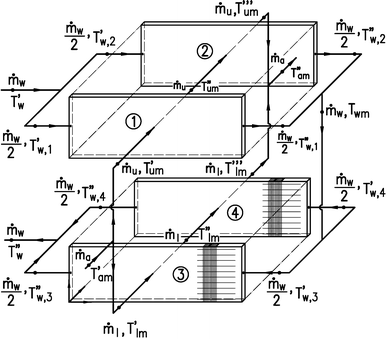
Flow diagram of two row cross-flow heat exchanger (automotive radiator) with two passes; 1 first tube row in upper pass, 2 second tube row in upper pass, 3 first tube row in lower pass, 4 second tube row in lower pass
- \(T_{um}^{\prime }\), \(T_{um}^{\prime \prime }\), \(T_{um}^{\prime \prime \prime }\) :
-
Average air temperature at inlet, after the first, and second row of tubes at the first (upper) pass, respectively, °C (Fig. 1)
- \(T_{w}\) :
-
Water temperature, °C
- \(T_{wm}\) :
-
Water outlet temperature after the first pass, °C
- \(T_{w}^{\prime }\), \(T_{w}^{\prime \prime }\) :
-
Water inlet and outlet temperature in the heat exchanger, respectively, °C
- \(T_{w,1}^{\prime }\), \(T_{w,2}^{\prime }\) :
-
Water temperature at the inlet to the first and second tube row in the first pass, °C (Fig. 1)
- \(T_{w,3}^{\prime }\), \(T_{w,4}^{\prime }\) :
-
Water temperature at the inlet to the first and second tube row in the second pass, °C (Fig. 1)
- \(T_{w,1}^{\prime \prime }\), \(T_{w,2}^{\prime \prime }\) :
-
Water temperature at the outlet from the first and second tube row in the first pass, °C (Fig. 1)
- \(T_{w,3}^{\prime \prime }\), \(T_{w,4}^{\prime \prime }\) :
-
Water temperature at the outlet from the first and second tube row in the second pass, °C (Fig. 1)
- U :
-
Overall heat transfer coefficient related to the outer surface of bare tube, W/(m2 K)
- \(\dot{V}_{a}^{\prime }\), \(\dot{V}_{w}^{\prime }\) :
-
Air and water volume flow rate before the heat exchanger, m3/s
- w a , w w :
-
Weighting factor for measured air and water temperature
- w max :
-
Average velocity in the minimum free flow area, m/s
- w 0 :
-
Average frontal flow velocity, m/s
- W :
-
Matrix of weighting factors
- x 1,…, x n :
-
Unknown parameters
- x :
-
Vector of unknown parameters
- x, y, z :
-
Cartesian coordinates
- δ f :
-
Fin thickness, m
- δ t :
-
Tube wall thickness, m
- ε :
-
Relative difference between water side and average heat flow rate, %
- η f :
-
Fin efficiency
- μ :
-
Dynamic viscosity, Pa s
- ν :
-
Kinematic viscosity, m2/s
- ξ :
-
Darcy–Weisbach friction factor
- ρ :
-
Density, kg/m3
- σ 2 a :
-
Variance of measured air temperature, K2
- σ 2 w :
-
Variance of measured water temperature, K2
- a :
-
Air
- f :
-
Fin
- in :
-
Inner
- o :
-
Outer
- t :
-
Tube
- w :
-
Water
- c :
-
Calculated
- (k):
-
Iteration number
- l :
-
Lower pass (second pass)
- m :
-
Measured
- u :
-
Upper pass
- −:
-
Average

References
Shah RK, Sekulić DP (2003) Fundamentals of heat exchanger design. Wiley, Hoboken
Dasgupta ES, Askar S, Ismail M, Fartaj A, Quaiyum MA (2012) Air cooling by multiport slabs heat exchanger: an experimental approach. Exp Thermal Fluid Sci 42:46–54
Park Y, Jacobi AM (2009) Air-side heat transfer and friction correlations for fat-tube louver–fin heat exchangers. ASME J Heat Transf 131:1801–1812
Welty JR, Wicks ChE, Wilson RE, Rorrer GL (2007) Fundamentals of momentum, heat, and mass transfer, 5th edn. Wiley, New York
McAdams WH (1954) Heat transmissions, 3rd edn. McGraw-Hill, New York
Dittus FW, Boelter LMK (1930) Heat transfer in automobile radiators of the tubular type. Univ Calif Publ Eng 2:443–461. Reprinted in: Int Commun Heat Mass Transf (1985) 12:3–22
Prandtl L (1910) Eine Beziehung zwischen Wärmeaustausch und Strömungswiderstand der Flüssigkeit. Z Physik 11:1072–1078
Petukhov BS, Genin AG, Kovalev SA (1974) Heat transfer in nuclear power plants. Atomizdat, Moscow (in Russian)
Prandtl L (1944) Führer durch die Strömungslehre. Vieweg und Sohn, Braunschweig
Lyon RN (1951) Liquid metal heat transfer coefficients. Chem Eng Prog 47:75–79
Kutateladze SS (1963) Fundamentals of heat transfer. Edward Arnold, London
Reichhardt H (1951) Vollständige Darstellung der turbulenten Geschwindigkeitsverteilung in glatten Leitungen. Zeitschrift für angewandte Mathematik und Mechanik 31:208–219
Gnielinski V (1975) Neue Gleichungen für den Wärme- und den Stoffübergang in turbulent durchströmten Rohren und Kanälen. Forsch Ingenieurwes 41:8–16
Gnielinski V (1976) New equations for heat and mass transfer in turbulent pipe and channel flow. Int Chem Eng 16:359–368
Wilson EE (1915) A basis for rational design of heat transfer apparatus. Trans ASME 37:47–70
Rose JW (2004) Heat-transfer coefficients, Wilson plots and accuracy of thermal measurements. Exp Thermal Fluid Sci 28:77–86
Kays WM, London AL (1984) Compact heat exchangers, 3rd edn. McGraw-Hill, New York
Wang CC, Webb RL, Chi KY (2000) Data reduction for air-side performance of fin-and-tube heat exchangers. Exp Thermal Fluid Sci 21:218–226
Taler D (2002) Theoretical and experimental analysis of heat exchangers with extended surfaces. Volume 25 Monograph 3, Cracow Branch of Polish Academy of Sciences, Automotive Committee, Cracow, Poland
Taler D (2004) Determination of heat transfer correlations for plate-fin-and-tube heat exchangers. Heat Mass Transf 40:809–822
Taler D (2004) Experimental determination of heat transfer and friction correlations for plate fin-and-tube heat exchangers. J Enhanc Heat Transf 11:183–204
Taler D, Trojan M, Taler J (2011) Mathematical modelling of tube heat exchangers with complex flow arrangement. Chem Process Eng 32:7–19
Taler D, Trojan M, Taler J (2011) Numerical modeling of cross-flow tube heat exchangers with complex flow arrangements. In: Ahsan A (ed) Evaporation condensation and heat transfer. InTech, Rijeka, pp 261–278
Taler D (2011) Direct and inverse heat transfer problems in dynamics of plate fin and tube heat exchangers. In: Belmiloudi A (ed) Heat transfer—mathematical modelling, numerical methods and information technology. InTech, Rijeka, pp 77–100
Krishnakumar K, John AK, Venkatarathnam G (2011) A review of transient test techniques for obtaining heat transfer design data of compact heat exchanger surfaces. Exp Thermal Fluid Sci 35:738–743
Jaremkiewicz M, Taler D, Sobota T (2009) Measuring transient temperature of the medium in power engineering machines and installations. Appl Therm Eng 29:3374–3379
Taler J (2007) Determination of local heat transfer coefficient from the solution of the inverse heat conduction problem. Forschung im Ingenieurwesen (Eng Res) 71:69–78
Taler J, Taler D (2012) Measurements of local heat flux and water-side heat transfer coefficient in water wall tubes. In: Kazi SN (ed) An overview of heat transfer phenomena. InTech, Rijeka, pp 3–34
Taler J, Taler D (2012) Measurement of heat flux and heat transfer coefficient. In: Cirimele G, D’Elia M (eds) Heat flux: processes, measurement techniques and applications. Nova Science Publishers, New York, pp 1–103
Junqi D, Jiangping C, Zhijiu C, Yimin Z, Wenfeng Z (2007) Heat transfer and pressure drop correaltions for the wavy fin and flat tube heat exchangers. Appl Therm Eng 27:2066–2073
Cuevas C, Makaire D, Dardenne L, Ngendakumana P (2011) Thermo-hydraulic characterization of a louvered fin and flat tube heat exchanger. Exp Thermal Fluid Sci 35:154–164
Taler D (2006) Measurement of pressure, velocity and flow rate of fluid. Publishing House of University of Science and Technology (AGH), Cracow, Poland (in Polish)
Seber GAF, Wild CJ (1989) Nonlinear regression. Wiley, New York
ESDU 86018 (1991) Effectiveness-NTU relationships for the design and performance evaluation of two-stream heat exchangers. Engineering Science Data Unit 86018 with amendment A, pp 92–107, ESDU International plc, London
Bevington PR (1969) Data reduction and error analysis for the physical sciences. McGraw-Hill, New York
Brandt S (1999) Data analysis. Statistical and computational methods for scientists and engineers, 3rd edn. Springer, Berlin
Coleman HW, Steele WG (2009) Experimentation, validation, and uncertainty analysis for engineers, 3rd edn. Wiley, Hoboken
Author information
Authors and Affiliations
Corresponding author
Rights and permissions
Open Access This article is distributed under the terms of the Creative Commons Attribution License which permits any use, distribution, and reproduction in any medium, provided the original author(s) and the source are credited.
About this article
Cite this article
Taler, D. Experimental determination of correlations for average heat transfer coefficients in heat exchangers on both fluid sides. Heat Mass Transfer 49, 1125–1139 (2013). https://doi.org/10.1007/s00231-013-1148-5
Received:
Accepted:
Published:
Issue Date:
DOI: https://doi.org/10.1007/s00231-013-1148-5