Mustafin varieties, moduli spaces and tropical geometry

Abstract

Mustafin varieties are flat degenerations of projective spaces, induced by a set of lattices in a vector space over a non-archimedean field. They were introduced by Mustafin (Math USSR-Sbornik 34(2):187, 1978) in the 70s in order to generalise Mumford’s groundbreaking work on the unformisation of curves to higher dimension. These varieties have a rich combinatorial structure as can be seen in pioneering work of Cartwright et al. (Selecta Math 17(4):757–793, 2011). In this paper, we introduce a new approach to Mustafin varieties in terms of images of rational maps, which were studied in Li (IMRN, 2017). Applying tropical intersection theory and tropical convex hull computations, we use this method to give a new combinatorial description of the irreducible components of the special fibers of Mustafin varieties. Finally, we outline a first application of our results in limit linear series theory.

1 Introduction

Mustafin varieties are flat degenerations of projective spaces induced by choosing a set of lattices in a K-vector space V. These objects were introduced by Mustafin in [22] in order to generalise Mumford’s groundbreaking work on uniformisation of curves to higher dimensions [21]. Since then they have been repeatedly studied under the name Deligne schemes (see e.g. [7, 10, 16]). By studying degenerations of projective spaces, we give a framework for the study of degenerations of projective subvarieties. In his original work, Mustafin studied the case of so-called convex subsets of ${\mathfrak {B}}_d$ as defined in Definition 2.12. An approach to study arbitrary subsets of ${\mathfrak {B}}_d$ was developed in [5], where the total space of this type of degenerations was named Mustafin variety for the first time. There it was proved that if the lattices in the subset of ${\mathfrak {B}}_d$ have diagonal form with respect to a common basis (i.e. they lie in the same apartment), the corresponding Mustafin variety is essentially a toric degeneration given by a mixed subdivision of a scaled simplex. These mixed subdivisions are beautiful combinatorial objects that are known to be equivalent to tropical polytopes and triangulations of products of simplices. For subsets of ${\mathfrak {B}}_d$ that do not obey this property some first structural results were proved. In this paper, we give a new combinatorial description of the special fibers of Mustafin varieties, which yields a complete classification of the irreducible components of special fibers of Mustafin varieties.

Let R be a discrete valuation ring, K the quotient field and k the residue field. We fix a uniformiser $\pi$. As an example take ${\mathbb {K}}={\mathbb {C}}((\pi ))$ as the ring of formal Laurent series over ${\mathbb {C}}$ with discrete valuation $v(\sum _{n\ge l}a_n\pi ^n)=l$ for $l\in {\mathbb {Z}}$ and $a_n\in {\mathbb {C}}$ with $a_l\ne 0$. Then $R=\{\sum _{n\ge l}a_n\pi ^n:l\in {\mathbb {Z}}_{\ge 0}\}$ and $k={\mathbb {C}}$. Moreover, let V be vector space of dimension d over K. We define ${\mathbb {P}}(V)=\mathrm {Proj}\mathrm {Sym}(V^*)$ as paramatrising lines through V. We call free R-modules $L\subset V$ of rank d lattices and define ${\mathbb {P}}(L)=\mathrm {Proj}\mathrm {Sym}(L^*)$, where $L^*=\mathrm {Hom}_R(L,R)$. Note, that we will mostly consider lattices up to homothety, i.e. $L\backsim L'$ if $L=c\cdot L'$ for some $c\in K^{\times }$. We denote the homothety class of L by [L].

Definition 1.1

(Mustafin varieties) Let $\Gamma =\{[L_1],\dots ,[L_n]\}$ be a set of lattice classes in V. Then ${\mathbb {P}}(L_1),\dots ,{\mathbb {P}}(L_n)$ are projective spaces over R whose generic fibers are canonically isomorphic to ${\mathbb {P}}(V)\simeq {\mathbb {P}}^{d-1}_{{\mathbb {K}}}$. The open immersions ${\mathbb {P}}(V)\hookrightarrow {\mathbb {P}}(L_i)$ give rise to a map

$$\begin{aligned} {\mathbb {P}}(V)\longrightarrow {\mathbb {P}}(L_1)\times _R\dots \times _R{\mathbb {P}}(L_n). \end{aligned}$$

We denote the closure of the image endowed with the reduced scheme structure by ${\mathcal {M}}(\Gamma )$. We call ${\mathcal {M}}(\Gamma )$ the associated Mustafin variety. Its special fiber ${\mathcal {M}}(\Gamma )_k$ is a scheme over k.

While the generic fiber of such a scheme is isomorphic to ${\mathbb {P}}^{d-1}$, the special fiber has many interesting properties.

The main tool in this paper is the study of closures of images of rational maps of the form

where W is a vector space over k of dimension d and $(W_i)_{i\in [n]}$ (with $[n]=\{1,\dots ,n\}$) is a tuple of sub-vector spaces $W_i\subset W$, such that $\bigcap W_i=\langle 0\rangle$ undertaken in [17]. We denote the closure of the above map by $X(W,W_1,\dots ,W_n)$.

We make the following assumption for the rest of the paper.

General Assumption

The residue field k is algebraically closed.

We proceed as follows: We denote by ${\mathfrak {B}}_d^0$ the set of lattice classes up to homothety in V. Let $\Gamma \subset {\mathfrak {B}}_d^0$ be a finite subset. To each lattice class $[L]\in {\mathfrak {B}}_d^0$, we associate a variety $X_{\Gamma ,[L]}$ of the form $X(k^d,W_1,\dots ,W_n)$ for some $W_i$ depending on [L] and $\Gamma$ (see Construction 3.1). We consider the convex hull $\mathrm {conv}(\Gamma )$ (see Definition 2.12), which is a set of lattices. Then we define a variety in $\left( {\mathbb {P}}_{k}^{d-1}\right) ^n$ as follows

$$\begin{aligned} \widetilde{{\mathcal {M}}}(\Gamma )=\bigcup _{[L]\in \mathrm {conv}(\Gamma )}X_{\Gamma ,[L]}. \end{aligned}$$

Moreover, when $\Gamma$ is contained in a single apartment of ${\mathfrak {B}}_d^0$, i.e. the lattices in $\Gamma$ are simulatenously diagonalisable, we identify a distinguished subset $V(\Gamma )$ of $\mathrm {conv}(\Gamma )$ and define

$$\begin{aligned} \widetilde{{\mathcal {M}}}^r(\Gamma )=\bigcup _{[L]\in V(\Gamma )}X_{\Gamma ,[L]}. \end{aligned}$$

The following is the main result of this paper.

Theorem 1.2

The irreducible components of the special fiber of Mustafin varieties are related to images of rational maps as follows:

• (1) If $\Gamma$ is a an arbitrary finite set of lattice classes, we have

  $$\begin{aligned} {\mathcal {M}}(\Gamma )_k=\widetilde{{\mathcal {M}}}(\Gamma ). \end{aligned}$$

• (2) If $\Gamma$ is a finite set of lattice classes in one apartment, we have

  $$\begin{aligned} {\mathcal {M}}(\Gamma )_k=\widetilde{{\mathcal {M}}}^r(\Gamma ). \end{aligned}$$

In each case, it is easy to see that the right hand side is contained in the special fiber of the Mustafin variety. For the other direction, we have to identify those lattice classes [L] that actually contribute an irreducible component. This is done by means of tropical intersection theory and multidegrees. Employing the techniques involved in the proof of Theorem 1.2, we obtain the following theorem.

Theorem 1.3

The varieties $X(k^d;W_1,\dots ,W_d)$ with $\mathrm {dim}(X(k^d;W_1,\dots ,W_d))=d-1$ classify all irreducible components of special fibers of Mustafin varieties, i.e.

• (1) Any irreducible component of the special fiber of a Mustafin variety is a variety of the form $X(k^d;W_1,\dots ,W_d)$ and

• (2) every variety $X(k^d;W_1,\dots ,W_n)$ with $\mathrm {dim}(X(k^d;W_1,\dots ,W_d))=d-1$ appears as an irreducible component of ${\mathcal {M}}(\Gamma )_k$ for some $\Gamma$.

Finally, we outline a first application of Theorem 1.2 in limit linear series theory.

This paper is structured as follows: In Sect. 2 we give a quick review of the tools needed to prove our theorems. In particular, we focus on the relation between the notions of tropical convexity and convexity in Bruhat–Tits buildings. We summarize some of the structural results for Mustafin varieties. Section 3 consists of the proof of Theorem 1.2 and Theorem 1.3. In Sect. 3.1, we construct the varieties $\widetilde{{\mathcal {M}}}(\Gamma )$ and $\widetilde{{\mathcal {M}}}^r(\Gamma )$. We prove Theorem 1.2 (1) in Sect. 3.2, Theorem 1.2 (2) in Sect. 3.3 and Theorem 1.3 in Sect. 3.4. In Sect. 4, we give a first application of our results in the theory of limit linear series.

2 Preliminaries

2.1 Tropical geometry

In this subsection, we recall some basics of tropical geometry required for this paper. Our main combinatorial tool in this paper is the notion of tropical convexity. We restrict ourselves to basic notions and results and refer to [20] Chapter 5.2 for a more detailed introduction. Our proof of Theorem 1.2 involves the identification of certain lattice points in so-called tropical convex hulls. We achieve this by means of tropical intersection theory of tropical linear spaces (i.e. tropical varieties of degree 1). Tropical intersection theory is a well-developed theory, for more details see e.g. [2] or [20].

2.1.1 Tropical convexity

In a sense tropical convexity is the notion of convexity over the tropical semiring $(\overline{{\mathbb {R}}},\oplus ,\odot )$, where $\overline{{\mathbb {R}}}={\mathbb {R}}\cup \{\infty \}$, $a\oplus b=\mathrm {min}(a,b)$ and $a\odot b=a+b$. We make this more precise in the following definition:

Definition 2.1

Let S be a subset of ${\mathbb {R}}^n$. We call S tropically convex, if for any choice $x,y\in S$ and $a,b\in {\mathbb {R}}$ we get $a\odot x\oplus b\odot y\in S$.

The tropical convex hull of a given subset V of ${\mathbb {R}}^n$ is given as the intersection of all tropically convex sets in ${\mathbb {R}}^n$ containing S. We denote the tropical convex hull of V by $\mathrm {tconv}(V)$.

This definition implies that every tropical convex set S is closed under tropical scalar multiplication. Thus, if $x\in S$ then so is $x+\lambda \mathbf{1 }$, where $\lambda \in {\mathbb {R}}$ and $\mathbf{1 }=(1,\dots ,1)$. Therefore, we will usually identify S with its image in $(n-1)$-dimension tropical torus .

We are interested in tropical convex hulls of a finite number of points. We begin by treating the case of two points.

Proposition 2.2

[8] The tropical convex hull of two points is a concatenation of at most $n-1$ ordinary line-segments. The direction of each line segment is a zero-one-vector.

The proof of this proposition is constructive and describes the points in the tropical convex hull explicitly. To give this explicit description for $x=(x_1,\dots ,x_n)$ and $y=(y_1,\dots ,y_n)$, we note that after relabelling and adding multiples of $\mathbf{1 }$, we may assume $0=y_1-x_1\le y_2-x_2\le \dots \le y_n-x_n$. Then the tropical convex hull consists of the concatenation of the lines connecting the following points:

$$\begin{aligned} x=&(y_1-x_1)\odot x\oplus y=(y_1,y_1-x_1+x_2,y_1-x_1+x_3,\dots ,y_1-x_1+x_n)\\&(y_2-x_2)\odot x\oplus y=(y_1,y_2,y_2-x_2+x_3,\dots ,y_2-x_2+x_n)\\&\cdots \cdots \\&(y_{n-1}-x_{n-1})\odot x\oplus y=(y_1,y_2,\dots ,y_{n-1},y_{n-1}-x_{n-1}+x_n)\\&(y_n-x_n)\odot x\oplus y=(y_1,\dots ,y_n) \end{aligned}$$

Some of these points might coincide, however they are always consecutive points on the line segment.

Next, we introduce a useful description of tropical convex hulls in terms of bounded cells of a tropical hyperplane arrangement: Fix a set $\Gamma =\{v_1,\dots ,v_n\}$ of , with $v_i=(v_{i1},\dots ,v_{in})$. Consider the standard tropical hyperplane at $v_i$ in the max-plus algebra:

Taking the common refinement, we obtain a polyhedral complex structure on , i.e. a subdivision into convex polyhedra, which we denote by $\mathrm {Tconv}(\Gamma )$. The support of the bounded cells of $\mathrm {Tconv}(\Gamma )$ is equal to $\mathrm {tconv}(\Gamma )$ (see e.g. chapter 5.2 in [20]). Moreover, we denote by $V(\Gamma )$ the set of vertices of the polyhedral complex $\mathrm {Tconv}(\Gamma )$.

In the following example we compute the tropical convex hull of three points in the tropical torus.

Example 2.3

We pick 3 points

$$\begin{aligned}&v_1=(0,-1,-2),\\&v_2=(0,-2,-4),\\&v_3=(0,-3,-6). \end{aligned}$$

Viewed as points in the tropical torus, we can identify these points with ${\widetilde{v}}_1=(-1,-2)$, ${\widetilde{v}}_1=(-2,-4)$ and ${\widetilde{v}}_3=(-3,-6)$. The tropical convex hull is illustrated in Fig. 1.

Remark 2.4

The tropical convex hull of finitely many points is also called a tropical polytope. Tropical polytopes can be thought of as tropicalisations of polytopes over the field of real Puiseux series ${\mathbb {R}}\{\{t\}\}$ (see Proposition 2.1 in [9]). One can generalise this notion to arbitrary tropical polyhedra and polyhedra over ${\mathbb {R}}\{\{t\}\}$, which in turn has applications in linear programming and complexity theory (see e.g. [1]).

2.1.2 Stable intersection

Tropical intersection theory is a well-developed field. In this paper, we will only intersect standard tropical hyperplanes, which is why we restrict ourselves to this case. A more general discussion can be found in [2, 20].

Definition 2.5

We fix n points $H_i$ be the standard tropical hyperplane at $v_i$. We denote the set-theoretic intersection of $H_1,\dots ,H_n$ by

$$\begin{aligned} H_1\cap \dots \cap H_n. \end{aligned}$$

Moreover, we define the stable intersection of $H_1,\dots ,H_n$ by

$$\begin{aligned} H_1\cap _{st}\dots \cap _{st}H_n=\lim _{\epsilon _1,\dots ,\epsilon _n\rightarrow 0}(H_1+\epsilon _1\cdot w_1)\cap \dots \cap (H_n+\epsilon _n\cdot w_n), \end{aligned}$$

where $+$ denotes the Minkowski sum and are generic vertices.

Fig. 1

The tropical convex hull of $v_1=(0,-1,-2)$, $v_2=(0,-2,-4)$ and $v_3=(0,-3,-6)$ in the tropical torus

Remark 2.6

We note, that there are several definitions of stable intersection in tropical geometry, which all turn out to be equivalent. For various viewpoints, we refer to [2, 14, 15, 25, 26].

Example 2.7

We illustrate the difference between set-theoretic intersection and stable intersection in the example of two lines not in tropical general position. The two lines in Fig. 2 intersect set-theoretically in the half-bounded line segment as illustrated in the upper right. However, the stable intersection only yields a single point as illustrated in the lower right.

Fig. 2

The difference between set-theoretic and stable intersection

In algebraic geometry, two general linear spaces of respective codimension $m_1$ and $m_2$ intersect in codimension $m_1+m_2$. A similar fact holds for tropical linear spaces. We first introduce a notion of points in tropical general position.

Definition 2.8

A square matrix $M\in {\mathbb {R}}^{r\times r}$ is tropically singular, if the minimum in

$$\begin{aligned} \mathrm {det}(M)=\bigoplus _{\sigma \in {\mathcal {S}}_r}m_{1\sigma (1)}\odot \cdots \odot m_{r\sigma (r)} \end{aligned}$$

is attained at least twice. A subset $\{m_1,\dots ,m_n\}\subset {\mathbb {R}}^{d}$ is in tropical general position, if every maximal minor of the matrix $((m_{ij})_{ij})$ is non-singular.

Let H be the standard tropical hyperplane at a point , then we denote the k-fold stable self-intersection (i.e. $\underbrace{H\cap _{st}\dots \cap _{st}H}_\text {\textit{k}\;times}$) by $H^k$. Moreover, for a polyhedral complex P of dimension d, we call its subcomplex $P'$ consisting of all polyhedra in P of dimension smaller or equal to k, where $k<d$, the k-skeleton of P. The following fact was proved in [3].

Lemma 2.9

Let H be the standard tropical hyperplane in at v. Its k-fold stable self-intersection $H^k$ is given by its $(d-k)$-skeleton.

Remark 2.10

Let be in tropically general position, let $m_1,\dots ,m_n\in {\mathbb {R}}_{\ge 0}$ and let $H_i$ be the standard tropical hyperplane at $v_i$. Then the stable intersection coincides with set-theoretic intersection in the sense that

$$\begin{aligned} H_1^{m_1}\cap _{st}\dots \cap _{st} H_n^{m_n}=H_1^{m_1}\cap \dots \cap H_n^{m_n}. \end{aligned}$$

We end this section, with the following proposition.

Proposition 2.11

Let and let $m_1,\dots ,m_n\in {\mathbb {R}}_{\ge 0}$, such that $\sum _{i=1}^nm_i=d-1$. Furthermore, let $H_i$ be standard tropical hyperplane at $v_i$, then

$$\begin{aligned} H_1^{m_1}\cap _{st}\dots \cap _{st} H_n^{m_n}=\{pt\} \end{aligned}$$

is exactly one point. Let $v_1,\dots ,v_n$ be in tropically general position, then the set-theoric intersection

$$\begin{aligned} H_1^{m_1}\cap \dots \cap H_n^{m_n}=\{pt\} \end{aligned}$$

coincides with the intersection product.

Proof

This follows immediately from theorem 5.7, theorem 5.8 in [2] and Lemma 2.9. $\square$

2.2 Bruhat-Tits buildings and tropical convexity

In this section, we recall some of the relations between Bruhat-Tits buildings and tropical convexity. For a short summary of Bruhat-Tits buildings, we refer to Section 2 of [5], for more details on the relation between buildings and tropical convexity see e.g. [27]. We denote the Bruhat-Tits building associated to $\mathrm {PGL}(V)$ by ${\mathfrak {B}}_d$. Furthermore, we denote by ${\mathfrak {B}}_d^0$ the set of lattice classes in V. We note that ${\mathfrak {B}}_d^0$ may be viewed as the set of integral points of ${\mathfrak {B}}_d$. We call two lattice classes [L], [M] in ${\mathfrak {B}}_d^0$ adjacent if there exist representatives $L'\in [L]$ and $M'\in [M]$, such that $\pi M'\subset L'\subset M'$.

We pick a basis $e_1,\dots ,e_d$ of V. The associated apartment A is the set of lattice classes in ${\mathfrak {B}}_d^0$ which are diagonal with respect to $e_1,\dots ,e_d$. We observe that the following map is a bijection:

(1)

For a subset $\Gamma \subset A$, we denote $\mathrm {Tconv}(\Gamma ):=\mathrm {Tconv}(f(\Gamma ))$ and $\mathrm {tconv}(\Gamma ):=\mathrm {tconv}(f(\Gamma ))$. Moreover, denote the set of lattices corresponding to the vertices of the polyhedral complex $\mathrm {Tconv}(\Gamma )$ by $V(\Gamma )$.

Definition 2.12

We call a subset $\Gamma \subset {\mathfrak {B}}_d^0$ convex if for $[L],[L']\in \Gamma$, any vertex of the form $[\pi ^aL\cap \pi ^bL']$ is also in $\Gamma$.

The convex hull $\mathrm {conv}(\Gamma )$ of a subset $\Gamma \subset {\mathfrak {B}}_d^0$ is the intersection of all convex sets containing $\Gamma$.

The following Lemma essentially goes back to [16], is a special case of Lemma 21 in [13] and can be found in this version as Lemma 4.1 in [5].

Lemma 2.13

Let $\Gamma \subset {\mathfrak {B}}_d^0$ be contained in one apartment A. The map in Eq. (1) induces a bijection between the lattices in $\mathrm {conv}(\Gamma )$ and the integral points in $\mathrm {tconv}(\Gamma )$.

Remark 2.14

We call a subset $\Gamma \subset {\mathfrak {B}}_d^0$ that is contained in the same apartment A in tropical general position, if the subset

is in tropical general position.

2.3 Images of rational maps

Let W be a d-dimensional vector space over k and let $(W_i)_{i=1}^n$ be a tuple of subvectorspaces of W with

$$\begin{aligned} \bigcap _{i=1}^nW_i=\langle 0\rangle . \end{aligned}$$

In [17], images of rational maps of the form

were studied. In particular, the Hilbert function and the multidegrees were computed. For every non-empty $I\subset [n]:=\{1,\dots ,n\}$ we define

$$\begin{aligned} d_I=\mathrm {dim}\bigcap _{i\in I}W_i. \end{aligned}$$

For every $h\in {\mathbb {Z}}_{\ge 0}$ we define M(h) to be the set

$$\begin{aligned} M(h)= & {} \{(m_1,\dots ,m_n)\in {\mathbb {Z}}_{\ge 0}^n:\sum _{i=1}^nm_i\\= & {} h\text { and }d-\sum _{i\in I}m_i>d_I\text { for every non-empty }I\subset [n]\}. \end{aligned}$$

Remark 2.15

There are several equivalent notions of the multidegree of a variety X in a product of projective spaces $\left( {\mathbb {P}}_k^{d-1}\right) ^n$. One possibility is to consider the multigraded Hilbert polynomial $h_X$: Let $x^u$ be a monomial of maximal degree in $h_X$ and $c_u$ be the coefficient. The multidegree function takes value $\frac{c_u}{u!}$ at u, where $u!=u_1!\cdots u_n!$.

Another way to describe the multidegree is to consider the intersection of X with a system of $u_i$ general linear equations in the i-th factor of , where we choose the $u_i$ such that the intersection is finite. Then the value of the multidegree function at $u=(u_1,\dots ,u_n)$ is the degree of this intersection product. For a more thorough introduction in terms of Chow classes, see e.g. [6]. We denote the set of multidegrees by

$$\begin{aligned} \mathrm {multDeg}(X)=\{u\in {\mathbb {Z}}_{\ge 0}^n:\text {the multidegree function is non-zero at }u\}. \end{aligned}$$

Theorem 2.16

[17] Assume k is algebraically closed. Set $p=\mathrm {max}\{h:M(h)\ne 0\}$. The dimension of $X(W,W_1,\dots ,W_n)$ is p. Its multidegree function takes value one at the integer vectors in M(p) and 0 otherwise. The Hilbert function of $X(W,W_1,\dots ,W_n)$ is

$$\begin{aligned} \sum _{S\subset M(p)}(-1)^{|S|-1}\prod _{j=1}^n{{u_i+\ell _{S,i}} \atopwithdelims ()\ell _{S,i}}, \end{aligned}$$

where the $u_i$ are the variables and $\ell _{S,i}$ is the smallest i-th components of all elements of S. Moreover, $X(W,W_1,\dots ,W_n)$ is Cohen-Macaulay.

We end this section with an example.

Example 2.17

Let $V={\mathbb {C}}^3$ and $e_1,e_2,e_3$ the standard basis. Moreover, let $V_1=(0),V_2=(e_2,e_3),V_3=(e_2,e_3)$ then

$$\begin{aligned} X=X(V,V_1,V_2,V_3)\cong {\mathbb {P}}^2\times {pt}\times {pt}. \end{aligned}$$

In the notation of Theorem 2.16, we see $p=2=\mathrm {dim}(X)$ with multidegree $\mathrm {multDeg}(X)=M(p)=M(2)=\{(2,0,0)\}$. The multidegree function takes value 1 at (2, 0, 0) and 0 else.

Let V and $e_1,e_2,e_3$ as above and let $V_1=(e_1), V_2=(e_1), V_3=(e_3)$. Furthermore, let $(x_{ij})_{i,j=1,2,3}$ be the coordinates on $\left( {\mathbb {P}}^2\right) ^3$, where $x_{1j},x_{2j},x_{3j}$ are the coordinates on the j-th factor. Then $X(V,V_1,V_2,V_3)$ is the subvariety of $\left( {\mathbb {P}}^2\right) ^3$ cut out be the ideal

$$\begin{aligned} I=(x_{11},x_{12},x_{33},x_{21}x_{32}-x_{31}x_{22}). \end{aligned}$$

In the notation of Theorem 2.16, we see $p=2=\mathrm {dim}(X)$ with multidegree $\mathrm {multDeg}(X)=M(p)=M(2)=\{(1,0,1),(0,1,1)\}$. The multidegree function takes value 1 at (1, 0, 1) and (0, 1, 1). The multidegree function takes value 0 else.

Moreover, we see that under the projection to the second and third factor of $\left( {\mathbb {P}}^2\right) ^3$, we have that $X(V,V_1,V_2,V_3)$ is mapped isomorphically to ${\mathbb {P}}^1\times {\mathbb {P}}^1$.

2.4 Mustafin varieties

Recall Definition 1.1 for a Mustafin variety ${\mathcal {M}}(\Gamma )$ associate to a subset $\Gamma \subset {\mathfrak {B}}_d^0$. In this subsection, we review the theory developed in [5], where many interesting structural results about ${\mathcal {M}}(\Gamma )$ and its special fiber were proved. We state results needed for our approach and refer to [5] for a more detailed discussion.

Proposition 2.18

([5, 22])

• (1) For a finite set of lattice classes $\Gamma \subset {\mathfrak {B}}_d^0$, the Mustafin variety ${\mathcal {M}}(\Gamma )$ is an integral, normal, Cohen-Macaulay scheme which is flat and projective over R. Its generic fiber is isomorphic to ${\mathbb {P}}^{d-1}_{{\mathbb {K}}}$ and its special fiber is reduced, Cohen-Macaulay and connected. All irreducible components are rational varieties and their number is at most ${n+d-2 \atopwithdelims ()d-1}$, where $n=|\Gamma |$.

• (2) If $\Gamma$ is a convex set in ${\mathfrak {B}}_d^0$, then the Mustafin variety is regular and its special fiber consists of n smooth irreducible components that intersect transversely. In this case the reduction complex of ${\mathcal {M}}(\Gamma )$ is induced by the simplicial subcomplex of ${\mathfrak {B}}_d$ induced by $\Gamma$.

• (3) If $\Gamma$ is contained in one apartment, the components of the special fiber correspond to maximal cells of the subdivision of the simplex $|\Gamma |\cdot \Delta _{d-1}$, which is dual to the polyhedral complex $\mathrm {Tconv}(\Gamma )$. If $\Gamma$ is in tropical general position, the irreducible components are products of projective linear spaces.

• (4) An irreducible component mapping birationally to the special fiber of ${\mathbb {P}}(L_i)$ is called a primary component. The other components are called secondary components. For each $i=1,\dots ,n$ there exists such a unique primary component. The primary components are pairwise distinct. A projective variety X arises as a primary component for some subset $\Gamma \subset {\mathfrak {B}}_d$ if and only if X is the blow-up of ${\mathbb {P}}_k^{d-1}$ at a collection of $n-1$ linear subspaces.

• (5) Let C be a secondary component of ${\mathcal {M}}(\Gamma )_k$. There exists an element v in $\mathrm {conv}(\Gamma )$, such that

  $$\begin{aligned} {\mathcal {M}}(\Gamma \cup \{v\})_k\longrightarrow {\mathcal {M}}(\Gamma )_k \end{aligned}$$

  restricts to a birational morphism ${\tilde{C}}\rightarrow C,$ where ${\tilde{C}}$ is the primary component of ${\mathcal {M}}(\Gamma \cup \{v\})_k$ corresponding to v.

Remark 2.19

We note that by e.g. [18, Proposition 4.4.16] the special fiber ${\mathcal {M}}(\Gamma )_k$ is equidimensional of dimension $d-1$. We note that the pairwise distinctness of primary components follows from [5, Theorem 5.3].

3 Special fibers of Mustafin varieties

The goal of this section is to prove Theorem 1.2 and Theorem 1.3.

3.1 Constructing the varieties $\widetilde{{\mathcal {M}}}(\Gamma )$ and $\widetilde{{\mathcal {M}}}^r(\Gamma )$

Let $\Gamma =\{L_1,\dots ,L_n\}\subset {\mathfrak {B}}_d^0$ be a finite set of lattice classes in V. The goal of this subsection is to construct the varieties $\widetilde{{\mathcal {M}}}(\Gamma )$ and $\widetilde{{\mathcal {M}}}^r(\Gamma )$. Our construction is motivated by the following way of choosing global coordinates on ${\mathcal {M}}(\Gamma )$ introduced in [5].

Consider the diagonal map

$$\begin{aligned} \Delta :{\mathbb {P}}(V)\longrightarrow {\mathbb {P}}(V)^n={\mathbb {P}}(V)\times _K\cdots \times _K{\mathbb {P}}(V). \end{aligned}$$

The image of $\Delta$ is the subvariety of ${\mathbb {P}}(V)^n$ cut out by the ideal generated by the $2\times 2$ minors of a matrix $X=(x_{ij})_{\begin{array}{c} i=1,\dots ,d\\ j=1,\dots ,n \end{array}}$ of unknowns, where the jth column corresponds to coordinates in the jth factor.

Start with an element $g\in \mathrm {GL}(V)$, it is represented by an invertible $n\times n$ matrix over K. It induces a dual map $g^t:V^*\rightarrow V^*$ and thus a morphism $g:{\mathbb {P}}(V)\rightarrow {\mathbb {P}}(V)$. For n elements $g_1,\dots ,g_n\in \mathrm {GL}(V)$, the image of

$$\begin{aligned} {\mathbb {P}}(V)\xrightarrow {\Delta }{\mathbb {P}}(V)^n\xrightarrow {g_1\times \dots \times g_n}{\mathbb {P}}(V)^n \end{aligned}$$

is the subvariety of ${\mathbb {P}}(V)^n$ cut out by the multihomogeneous prime ideal

$$\begin{aligned} I_2((g_1^{-1},\dots ,g_n^{-1})(X))\subset K[X], \end{aligned}$$

where $(g_1^{-1},\dots ,g_n^{-1})(X)$ is the matrix whose jth column is given by

$$\begin{aligned} g_j^{-1}\begin{pmatrix}x_{1j}\\ \vdots \\ x_{dj}\end{pmatrix}. \end{aligned}$$

Consider a reference lattice $L=Re_1+\cdots +Re_d$. For any set $\Gamma =\{[L_1],\dots ,[L_n]\}$ of lattice classes in ${\mathfrak {B}}_d^0$, we choose $g_i$, such that $g_iL_i=L$ for all i. The following diagram commutes:

It follows immediately that the Mustafin Variety ${\mathcal {M}}(\Gamma )$ is isomorphic to the subscheme of ${\mathbb {P}}(L)^n\cong ({\mathbb {P}}^{d-1}_R)^n$ cut out by the multihomogeneous ideal $I_2\left( (g_1^{-1},\dots ,g_n^{-1})(X)\right) \cap R[X]$ in R[X].

Motivated by this choice of coordinates on ${\mathcal {M}}(\Gamma )$, we proceed with the following construction.

Construction 3.1

Let $\Gamma =\{[L_1],\dots ,[L_n]\}\subset {\mathfrak {B}}_d^0$ be a finite set of lattices. Moreover, let $L=Re_1+\dots +Re_d$ be a lattice in V for $e_1,\dots ,e_d\in V$. As in the choice of coordinates on ${\mathcal {M}}(\Gamma )$ above, we let $g_1,\dots ,g_n\in \mathrm {GL}(V)$, such that $g_iL_i=L$. We denote ${\underline{g}}=(g_1,\dots ,g_n)$. In the following, we construct a variety $X_{[L],{\underline{g}}}$ over k associated to this data.

• (a) To begin with, we construct for open immersion $g_i:{\mathbb {P}}(V)\rightarrow {\mathbb {P}}(L)$ a continuation to a rational map

  $$\begin{aligned} g_i':{\mathbb {P}}(L)\dashrightarrow {\mathbb {P}}(L) \end{aligned}$$

  with

  $$\begin{aligned} {g_i'}_{|{\mathbb {P}}(V)}\equiv g_i. \end{aligned}$$

  (2)

  In order to construct this continuation, we note that since L is a free rank d lattice, we have that $e_1,\dots ,e_d$ is a basis of V. Let $G_i$ be the matrix representation of $g_i$ with respect to the basis $e_1,\dots ,e_d$. We define

  $$\begin{aligned} s_i=\mathrm {min}_{\mu ,\nu =1,\dots ,d}(\mathrm {val}((G_i)_{\mu \nu })) \end{aligned}$$

  and $G_i'=\pi ^{-s_i}G_i$. Then $G_i'$ is defined over R, but $\pi ^{-1}G_i'$ is not. We first note that $G_i'$ and $G_i$ induce the same morphism

  $$\begin{aligned} {\mathbb {P}}(V)\xrightarrow {g_i}{\mathbb {P}}(L) \end{aligned}$$

  since they lie in the same equivalence class of $\mathrm {PGL}(V)$. Moreover, $G_i'$ induces a linear map $g_i':L\rightarrow L$, which yields the desired rational map

  

  (3)

  satisfying Eq. (2). We note that $g_i'$ is independent of the choice of basis $e_1,\dots ,e_d$ and the representative of [L].

• (b) Secondly, we observe that by the above considerations, we have constructed a continuation of ${\mathbb {P}}(V)\xrightarrow {(g_1,\dots ,g_n)\circ \Delta }{\mathbb {P}}(L)^n$ to the rational map

  

  We denote by $(g_i')_k:{\mathbb {P}}(L)_k\dashrightarrow {\mathbb {P}}(L)_k$ the rational map over the special fibers induced by Eq. (3). Then, the map over the special fibers induced by $F_{[L],{\underline{g}}}$ is given by

  

  i.e. we have

  $$\begin{aligned} \left( F_{[L],{\underline{g}}}\right) _{|{\mathbb {P}}(L)_k}\equiv f_{[L],{\underline{g}}}. \end{aligned}$$

  We define the variety

  $$\begin{aligned} X_{[\Gamma ],{\underline{g}}}:=\overline{\mathrm {Im}(f_{[L],{\underline{g}}})}. \end{aligned}$$

Remark 3.2

We note that in the notation of Construction 3.1, the basis $e_1,\dots ,e_d$ of L induces a basis $e_1',\dots ,e_d'$ on $k^d\equiv L\,\mathrm {mod}\,\pi$. With respect to this basis, the map $(g_i')_k:{\mathbb {P}}(L)_k\rightarrow {\mathbb {P}}(L)_k$ is given by the matrix $G_i'\,\mathrm {mod}\,\pi$.

In Construction 3.1, our construction of $X_{\Gamma ,{\underline{g}}}$ depends on choices of elements $g_i\in \mathrm {GL}(V)$, such that $g_iL_i=L$. In the following lemma, we show that while the construction depends on these choices, the variety itself does not.

Lemma 3.3

Let L and $\Gamma$ given as in Construction 3.1. Moreover, let ${\underline{g}}=(g_1,\dots ,g_n)\in \mathrm {GL}(V)^n$ and ${\underline{h}}=(h_1,\dots ,h_n)\in \mathrm {GL}(V)^n$, such that $g_iL_i=h_iL_i=L$. Then, we have

$$\begin{aligned} X_{[L],{\underline{g}}}\cong X_{[L],{\underline{h}}}. \end{aligned}$$

Therefore, we will also denote the variety constructed in Construction 3.1 by $X_{[L],\Gamma }$.

Proof

We first observe that since $g_iL_i=h_iL_i=L$, we have for $l_i=h_i\circ g_i^{-1}$ that $l_iL=L$. Thus, we obtain isomorphisms ${\mathbb {P}}(L)\xrightarrow {l_i}{\mathbb {P}}(L)$, which induce isomorphisms ${\mathbb {P}}(L)_k\xrightarrow {(l_i)_k}{\mathbb {P}}(L)_k$ over the special fibers. In particular, we obtain an isomorphism

$$\begin{aligned} {\mathbb {P}}(L)^n\xrightarrow {(l_1,\dots ,l_n)}{\mathbb {P}}(L)^n \end{aligned}$$

and again an isomorphism over the special fiber

In the notation of Construction 3.1, we consider the following commutative diagram

which induces the commutative diagram

As the vertical arrow in Eq. (4) is an isomorphism, the lemma follows. $\square$

We are now ready to define $\widetilde{{\mathcal {M}}}(\Gamma )$ and $\widetilde{{\mathcal {M}}}^r(\Gamma )$.

Definition 3.4

We fix a reference lattice L, let $\Gamma =\{[L_1],\dots ,[L_n]\}\subset {\mathfrak {B}}_d^0$ and $g_i\in \mathrm {GL}(V)$ such that $g_iL_i=L$. Moreover, for any $[L']\in {\mathfrak {B}}_d^0$ with representative $L'$, we choose $h_{L'}\in GL(V)$ with $h_{L'}L'=L$.

For any $[L']\in {\mathfrak {B}}_d^0$, we consider the linear isomorphisms

$$\begin{aligned} {\tilde{h}}_{L'}:{\mathbb {P}}(L')^n\xrightarrow {(h_{L'},\dots ,h_{L'})}{\mathbb {P}}(L)^n. \end{aligned}$$

Then, for ${\underline{g}}_{[L']}=(h_{L'}^{-1}g_1,\dots ,h_{L'}^{-1}g_n)$ we define

$$\begin{aligned} \widetilde{{\mathcal {M}}}(\Gamma )=\bigcup _{[L']\in \mathrm {conv}(\Gamma )}{\tilde{h}}_{L'}(X_{[L'],{\underline{g}}_{[L']}}). \end{aligned}$$

Moreover, when $\Gamma$ is contained in a single apartment, we define

$$\begin{aligned} \widetilde{{\mathcal {M}}}^r(\Gamma )=\bigcup _{[L']\in V(\Gamma )}{\tilde{h}}_{L'}(X_{[L'],{\underline{g}}_{[L']}}). \end{aligned}$$

Before relating $\widetilde{{\mathcal {M}}}(\Gamma )$ and $\widetilde{{\mathcal {M}}}^r(\Gamma )$ to ${\mathcal {M}}(\Gamma )_k$, we make the following important remarks.

Remark 3.5

• (1) By a similar argument as in the proof of Lemma 3.3, we see that $\widetilde{{\mathcal {M}}}(\Gamma )$ and $\widetilde{{\mathcal {M}}}^r(\Gamma )$ do not depend on the reference lattice L or the chosen elements $g_i,g_{j,[L']}\in \mathrm {GL}(V)$.

• (2) In the situation of Construction 3.1, let the subset $\Gamma =\{[L_1],\dots ,[L_n]\}\subset {\mathfrak {B}}_d^0$ be contained in one apartment A associated to the basis $e_1,\dots ,e_d$. Let L be lattice with $[L]\in A$, then we may choose the following representations

  $$\begin{aligned}&L=\pi ^{m_1}Re_1+\dots +\pi ^{m_d}Re_d\quad \text {and}\\&L_i=\pi ^{n_1^i}Re_1+\dots +\pi ^{n_d^i}Re_d. \end{aligned}$$

  Therefore, we may choose the matrices $G_i$ in Construction 3.1 as

  $$\begin{aligned} \begin{pmatrix} \pi ^{m_1-n_1^i} &{} &{}\\ &{}\ddots &{} \\ &{} &{} \pi ^{m_d-n_d^i} \end{pmatrix} \end{aligned}$$

  Then, we obtain $G_i'=\pi ^{-s_i}G_i$, where $s_i=\mathrm {min}_{j=1,\dots ,d}(m_j-n_j^i)$. In particular, by Remark 3.2 the map $f_{[L],{\underline{g}}}$ is represented by $(H_1,\dots ,H_n)$, where

  $$\begin{aligned} H_i=G_i'\,\mathrm {mod}\,\pi =\begin{pmatrix} a_1 &{} &{}\\ &{} \ddots &{}\\ &{} &{} a_d \end{pmatrix}, \end{aligned}$$

  where

  $$\begin{aligned} a_j=1, \text { if }m_j-n_j^i=\min _{l=1,\dots ,d}(m_l-n_l^i) \end{aligned}$$

  and $a_j=0$ else. (see Example 3.6).

• (3) The key observation for the proof of Theorem 1.2 is that the maps $f_{[L],{\underline{g}}}$ factorise as follows:

  

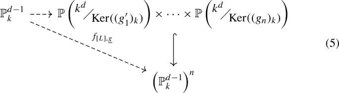
  Thus, each variety $X_{[L],\Gamma }$ is a variety of the form $X(k^d,W_1,\dots ,W_n)$, where $W_i=\mathrm {ker}((g_i')_k)$. Note that $\bigcap _{i=1}^nW_i$ might not be trivial. However, by Remark 2.19 the components of ${\mathcal {M}}(\Gamma )_k$ are equidimensional. The vertices with $\bigcap _{i=1}^nW_i\ne \langle 0\rangle$ contribute varieties of lower dimension and thus are contained in an irreducible component by Lemma 3.7. This irreducible component is contributed by a vertex satisfying $\bigcap _{i=1}^nW_i=\langle 0\rangle$.

Before we prove Theorem 1.2, we illustrate our construction in the following example:

Example 3.6

By Lemma 2.13, there is a natural correspondence between lattice points in and lattice classes in V over R. In Example 2.2 in [5], the special fiber of the Mustafin variety corresponding to the vertices in Example 2.3 was computed to be the union of the following irreducible components

$$\begin{aligned} {\mathbb {P}}^2\times & {} pt \times pt,\ pt \times {\mathbb {P}}^2\times pt,\ pt \times pt\times {\mathbb {P}}^2,\ {\mathbb {P}}^1\\\times & {} {\mathbb {P}}^1\times pt,\ {\mathbb {P}}^1\times pt\times {\mathbb {P}}^1 ,\ pt\times {\mathbb {P}}^1\times {\mathbb {P}}^1 \end{aligned}$$

Our construction yields the same variety as seen in the following computations. For $v=v_3$, we obtain the map

$$\begin{aligned} \begin{pmatrix}1 &{} 0 &{} 0\\ 0 &{} \pi ^2 &{} 0\\ 0 &{} 0 &{} \pi ^4 \end{pmatrix}\times \begin{pmatrix} 1 &{} 0 &{} 0\\ 0 &{} \pi &{} 0\\ 0 &{} 0 &{} \pi ^2\end{pmatrix}\times \mathrm {id}\end{aligned}$$

Modding out $\pi$, we immediately see that

$$\begin{aligned} X_{[L],\Gamma }=pt\times pt \times {\mathbb {P}}^2, \end{aligned}$$

where [L] is the lattice class corresponding to $v_3$. Analogously, we obtain $pt \times {\mathbb {P}}^2\times pt$ and ${\mathbb {P}}^2 \times pt\times pt$ for $v=v_2$ and $v=v_1$ respectively.

For $v=(0,-1,-4)$, we obtain the map

$$\begin{aligned} \begin{pmatrix}1 &{} 0 &{} 0\\ 0 &{} 1 &{} 0\\ 0 &{} 0 &{} \pi ^2 \end{pmatrix}\times \begin{pmatrix}\pi &{} 0 &{} 0\\ 0 &{} 1 &{} 0\\ 0 &{} 0 &{} \pi \end{pmatrix}\times \begin{pmatrix}\pi ^2 &{} 0 &{} 0\\ 0 &{} 1 &{} 0\\ 0 &{} 0 &{} 1\end{pmatrix}. \end{aligned}$$

Modding out $\pi$, we immediately see that

$$\begin{aligned} X_{[L],\Gamma }={\mathbb {P}}^1\times pt\times {\mathbb {P}}^1, \end{aligned}$$

where once again [L] is the lattice class corresponding to v. Analogously, we obtain ${\mathbb {P}}^1\times {\mathbb {P}}^1\times pt$ and $pt\times {\mathbb {P}}^1\times {\mathbb {P}}^1$ for $v=(0,-1,-3)$ and $v=(0,-2,-4)$ respectively.

The following Lemma implies the easier containment for the equalities of Theorem 1.2.

Lemma 3.7

In the notation of Construction 3.1, for any lattice class $[L]\in {\mathfrak {B}}_d^0$, the following relation holds:

$$\begin{aligned} X_{[L],{\underline{g}}}\subset {\mathcal {M}}(\Gamma )_k. \end{aligned}$$

Moreover, the variety $X_{[L],{\underline{g}}}$ is an irreducible component of ${\mathcal {M}}(\Gamma )_k$ if and only if

$$\begin{aligned} \mathrm {dim}(X_{[L],{\underline{g}}})=\mathrm {dim}({\mathcal {M}}(\Gamma )_k). \end{aligned}$$

Proof

To prove the first assertion, we observe that

$$\begin{aligned} X_{[L],{\underline{g}}}=\overline{F_{[L],{\underline{g}}}\left( \overline{{\mathbb {P}}(V)}\right) \cap {\mathbb {P}}(L)_k^n}, \end{aligned}$$

while by the discussion at the beginning of this subsection, we have

$$\begin{aligned} {\mathcal {M}}(\Gamma )_k=\overline{F_{[L],{\underline{g}}}({\mathbb {P}}(V))}\cap {\mathbb {P}}(L)^n_k=\overline{\overline{F_{[L],{\underline{g}}}({\mathbb {P}}(V))}\cap {\mathbb {P}}(L)^n_k}. \end{aligned}$$

Since $F_{[L],{\underline{g}}}$ is a continuous map, we have that $F_{[L],{\underline{g}}}\left( \overline{{\mathbb {P}}(V)}\right) \subset \overline{F_{[L],{\underline{g}}}({\mathbb {P}}(V))}$. The second assertion follows immediately by Remark 2.19. $\square$

To end this subsection, we give a purely tropical description of the map $f_{[L],{\underline{g}}}$, whenever $\Gamma$ is a finite set in one apartment A and $[L]\in A$. In fact, we associate such a map and thus a variety to any finite subset of the tropical torus .

Construction 3.8

Let be a finite subset of the tropical torus, where $v_i=(v_i^1,\dots ,v_i^n)$. For any , where $v=(v^1,\dots ,v^n)$, we define rational maps

$$\begin{aligned} f_{[v],\Gamma }:{\mathbb {P}}_k^{d-1}\dashrightarrow ({\mathbb {P}}_k^{d-1})^n \end{aligned}$$

where the map $g_j'$ to the jth factor is given by

$$\begin{aligned} \begin{pmatrix} a_1 &{} &{}\\ &{} \ddots &{}\\ &{} &{} a_d \end{pmatrix}, \end{aligned}$$

where $a_m=1$, if $v_j^m-v^m=\mathrm {min}_{l}(v_j^l-v^l)$ and $a_m=0$ otherwise. We further define $X_{[v],\Gamma }=\overline{\mathrm {Im}(f_{[v],\Gamma })}$ and define

$$\begin{aligned} {\widetilde{M}}^r(\Gamma )=\bigcup _{[v]\in V(\Gamma )}X_{v,\Gamma }. \end{aligned}$$

For $\Gamma '=\{[L_1],\dots ,[L_n]\}\subset {\mathfrak {B}}_d^0$ be finite set of lattice classes in one apartment A and let $\Gamma =\{[v_1],\dots ,[v_n]\}$ be the corresponding subset of the tropical torus, then by the discussion in Remark 3.5 (2), we have

$$\begin{aligned} {\widetilde{M}}(\Gamma )={\widetilde{M}}(\Gamma ')\,\,\mathrm {and}\,\,{\widetilde{M}}^r(\Gamma )={\widetilde{M}}^r(\Gamma '). \end{aligned}$$

3.2 Proof of Theorem 1.2 (1)

This subsection is devoted to proving Theorem 1.2 (1). The strategy of the proof is to show that

$$\begin{aligned} {\mathcal {M}}(\Gamma )_k=\widetilde{{\mathcal {M}}}(\Gamma ) \end{aligned}$$

for convex subset of lattice classes $\Gamma$ and recover the general case by using [5, Lemma 2.4].

We fix a convex subset $\Gamma =\{[L_1],\dots ,[L_n]\}\subset {\mathfrak {B}}_d^0$. By Proposition 2.18 (2), the special fiber consists of n irreducible components. Thus, in order to prove

$$\begin{aligned} {\mathcal {M}}(\Gamma )_k=\widetilde{{\mathcal {M}}}(\Gamma ) \end{aligned}$$

we need to show that $\widetilde{{\mathcal {M}}}(\Gamma )$ has n pairwise distinct irreducible components.

Let $[L_i]\in \Gamma$ and choose $g_1,\dots ,g_n\in \mathrm {GL}(V)$ with $g_jL_j=L_i$. In particular, we may choose $g_i=\mathrm {id}$. In the notation of Construction 3.1, we consider for each $j\in [n]$ the following commutative diagram

where $p_j$ denotes the projection to the j-th factor. There is a dense open subset $U_j\subset {\mathbb {P}}(L_i)_k$, such that ${p_j\circ f_{[L_i],{\underline{g}}}}_{|U}\equiv (g_j')_k$.

In particular, we obtain ${p_j\circ f_{[L_i],{\underline{g}}}}_{|U}\equiv \mathrm {id}$. In other words, for $j=i$ the vertical arrow is a birational map between $X_{[L_i],{\underline{g}}}$ and ${\mathbb {P}}(L_i)$. Therefore, we have that $\mathrm {dim}(X_{[L_i],{\underline{g}}})=d-1$. Thus, by Lemma 3.7 it follows that $X_{[L_i],{\underline{g}}}$ is an irreducible component of ${\mathcal {M}}(\Gamma )_k$, which is in fact the i-th primary component. Since by Proposition 2.18 (4), the primary components are pairwise distinct, this completes the proof of Theorem 1.2 (1) for convex sets $\Gamma$.

Now, let $\Gamma$ be any subset of ${\mathfrak {B}}_d^0$. Then by lemma 2.4 of [5], we can compare the special fibers of ${\mathcal {M}}(\Gamma )$ and ${\mathcal {M}}(\mathrm {conv}(\Gamma ))$: Let C be an irreducible component of ${\mathcal {M}}(\Gamma )_k$, then there exists a unique irreducible component ${\tilde{C}}$ of ${\mathcal {M}}(\mathrm {conv}(\Gamma ))_k$ which projects onto C under

$$\begin{aligned} p_{\Gamma }:\prod _{L\in \mathrm {conv}(\Gamma )}{\mathbb {P}}(L)_k\rightarrow \prod _{L\in \Gamma }{\mathbb {P}}(L)_k. \end{aligned}$$

The key idea in proving Theorem 1.2 (1) for arbitrary subsets $\Gamma \subset {\mathfrak {B}}_d^0$ is to observe that Construction 3.1 commutes with projections. More precisely, let L be any lattice, $\Gamma '=\mathrm {conv}(\Gamma )=\{[L_1],\dots ,[L_n],[L_{n+1}],\dots ,[L_\nu ]\}$ and we denote $g_1,\dots ,g_\nu$ with $g_iL_i=L$. Moreover, we set ${\underline{g}}=(g_1,\dots ,g_\nu )$ and $\tilde{{\underline{g}}}=(g_1,\dots ,g_n)$ the following diagramm commutes:

We have proved that

$$\begin{aligned} {\mathcal {M}}(\Gamma ')_k=\bigcup _{L\in \Gamma '}X_{[L],\Gamma '} \end{aligned}$$

To see that

$$\begin{aligned} {\mathcal {M}}(\Gamma )_k=\bigcup _{L\in \Gamma '}X_{[L],\Gamma '} \end{aligned}$$

we fix an irreducible component $C\in {\mathcal {M}}(\Gamma )_k$ and denote the component which projects onto it by ${\widetilde{C}}$. By the previous discussion, there exists a unique lattice class $[L_C]\in \Gamma '$, such that ${\widetilde{C}}=X_{[L_C],\Gamma '}$. By the commutative diagram, we see that $C=p_{\Gamma }({\widetilde{C}})=X_{[L_C],\Gamma }$. Thus, every component C of ${\mathcal {M}}(\Gamma )_k$ is contained in $\widetilde{{\mathcal {M}}}(\Gamma )$, which together with Lemma 3.7 completes the proof. $\square$

3.3 Proof of Theorem 1.2 (2)

In this subsection, we prove the equality of the variety $\widetilde{{\mathcal {M}}}^r(\Gamma )$ defined in Definition 3.4 and the special fiber of the Mustafin variety ${\mathcal {M}}(\Gamma )$ defined in Definition 1.1 when $\Gamma$ is contained in one apartment. We have already seen that $\widetilde{{\mathcal {M}}}^r(\Gamma )\subset {\mathcal {M}}(\Gamma )_k$ in Lemma 3.7. To see the other direction, we compare the multidegrees. Since ${\mathcal {M}}(\Gamma )_k$ is a flat degeneration of the diagonal of $({\mathbb {P}}^{d-1})^n$, we know (see e.g. [7]) that

$$\begin{aligned} \mathrm {multDeg}({\mathcal {M}}(\Gamma )_k)=\left\{ (m_1,\dots ,m_n)\in {\mathbb {Z}}_{\ge 0}^n:\;\sum _{i=1}^nm_i=d-1\right\} . \end{aligned}$$

(6)

Moreover, the multidegree function takes value 1 at each multidegree. It is easy to see that $|\mathrm {multDeg}({\mathcal {M}}(\Gamma )_k)|={{n+d-2}\atopwithdelims (){d-1}}$.

If we prove that the same holds true for the multidegree function of $\widetilde{{\mathcal {M}}}^r(\Gamma )$, we can deduce equality. Thus, we have to prove two statements:

• The special fiber of the Mustafin variety and the variety we constructed have the same multidegrees: $\mathrm {multDeg}(\widetilde{{\mathcal {M}}}^r(\Gamma ))=\mathrm {multDeg}({\mathcal {M}}(\Gamma )_k)$, where we know the right hand side of the equation.

• The multidegree function takes value one at each $(m_1,\dots ,m_n)\in \mathrm {multDeg}(\widetilde{{\mathcal {M}}}^r(\Gamma ))$.

The basic idea is as follows: For every tuple $(m_1,\dots ,m_n)$ as above, we find a vertex in $\mathrm {Tconv}(\Gamma )$ whose associated variety contributes multidegree $(m_1,\dots ,m_n)$. We use basic tropical intersection theory. By our method, it is immediate that there is only one vertex that can contribute a variety of this multidegree.

We begin by treating the case of lattice classes being in tropical general position. The case of arbitrary subsets $\Gamma$ will follow using stable intersection.

3.3.1 $\Gamma$ in tropical general position

For a finite subset $\Gamma \subset {\mathfrak {B}}_d^0$ in tropical general position, the cardinality of $V(\Gamma )$ is ${{n+d-2}\atopwithdelims (){d-1}}$ as proved in [8]. This coincides with the cardinality of $\mathrm {multDeg}({\mathcal {M}}(\Gamma )_k)$. Therefore, the natural candidates for the correct multidegrees are the elements of $V(\Gamma )$.

We begin by describing the lattices in $V(\Gamma )$ and start by defining a map

$$\begin{aligned} \begin{aligned} C:V(\Gamma )&\longrightarrow \left\{ (m_1,\dots ,m_n)\in {\mathbb {Z}}_{\ge 0}^n|\sum _{i=1}^nm_i=d-1\right\} \\v&\longmapsto (C(v)_1,\dots ,C(v)_n), \end{aligned} \end{aligned}$$

(7)

where $C(v)_i$ is the largest k, such that v lies in the codimension k-skeleton of the hyperplane rooted at the lattice class $[L_i]\in \Gamma$. It is not obvious why this map is well defined. This is where tropical intersection theory comes into play.

As mentioned before the cardinality of $V(\Gamma )$ coincides with the number of tuples $(m_1,\dots ,m_n)\in \mathrm {multDeg}({\mathcal {M}}(\Gamma )_k)$. If we construct one pre-image for each such tuple under the map C in Eq. (7), we are done. Let $(m_1,\dots ,m_n)$ be such a tuple. We identify a vertex in $V(\Gamma )$ as follows: Let $\Gamma =\{[L_1],\dots ,[L_n]\}$ and $v_1,\dots ,v_n$ the corresponding vertices in the tropical torus. We intersect the standard max-hyperplanes $H_i$ at $v_i$

$$\begin{aligned} H_1^{m_1}\cap _{st}\dots \cap _{st}H_n^{m_n}=H_1^{m_1}\cap \dots \cap H_n^{m_n}=\{v\} \end{aligned}$$

as in Proposition 2.11. This intersection point v is a an element of $V(\Gamma )$ and thus C is well-defined. In fact we have proved that the map C is bijective.

Now, we study the maps $f_{[v],\Gamma }=((g_1')_k,\dots ,(g_n')_k)$ as in Construction 3.8, in particular the associated numerical data

$$\begin{aligned} d_I=\mathrm {dim}\bigcap _{i\in I}\mathrm {ker}(g_i')_k. \end{aligned}$$

Lemma 3.9

Let $v\in \mathrm {tconv}(v_1,\dots ,v_n)$ such that v is contained in the codimension $m_i$ skeleton at $v_i$, but not in the codimension $m_i+1$ skeleton. Then,

$$\begin{aligned} \mathrm {dim}\mathrm {Ker}((g_i')_k)=d-1-m_i, \end{aligned}$$

where $(g_i')_k$ is the map to the i-th factor in Construction 3.8.

Proof

We look at $v_i-v=(v_{i0}-v_1,\dots ,v_{id}-v_d)$. Since v is contained in the codimension $m_i$ skeleton at $v_i$, but not in the codimension $m_i+1$ skeleton, the minimum of $v_{i0}-v_1,\dots ,v_{id}-v_d$ is attained $m_i+1$ times. As described in Construction 3.8, the map $(g_i')_k$ over the special fiber is given by

$$\begin{aligned} D=\begin{pmatrix}a_1 &{} &{} \\ &{} \ddots &{}\\ &{} &{} a_d\end{pmatrix}, \end{aligned}$$

where $a_j=1,$ if the minimum is attained at $v_{ij}-v_1$ and $a_j=0$ else. Thus, the dimension of the kernel of the map is given by $d-(m_i+1)$. $\square$

Lemma 3.10

Let v be a vertex of $\mathrm {Tconv}(v_1,\dots ,v_n)$, where the $v_i$ are in tropical general position. For any $I\subset \{1,\dots ,n\}$, we have

$$\begin{aligned} d_I=\bigcap _{i\in I}\mathrm {ker}(g_i')=d-1-\sum _{i\in I}m_i, \end{aligned}$$

where $g_i'$ is the map to the i-th factor in Construction 3.8 and $m_i=C(v)_i$.

Proof

Let v be a vertex of $\mathrm {Tconv}(v_1,\dots ,v_n)$ as before. Moreover, let $C_i$ be the codimension $m_i$ cone of the hyperplane at $v_i$ in which v is contained.

Let $H_I$ be the intersection of the $C_i$ for $i\in I$. We can describe each $C_i$ as follows:

for some $J_i\subset \{1,\dots ,d\}$ such that $|J_i|=m_i+1$. Since $v_1,\dots ,v_n$ are in general position, $(v_i)_{i\in I}$ are in general position as well. Moreover, with the same arguments as before, the codimension $m_i$ skeleta at $v_i$ for $i\in I$ intersect in codimension $\sum _{i\in I}m_i$. Thus, we have

$$\begin{aligned} \left| \bigcup _{i\in I}J_i\right| =\sum _{i\in I}m_i+1. \end{aligned}$$

Now the kernel of the map $(g_i')_k$ is generated by the basis vectors $e_j$, such that $j\notin J_i$. Thus, the intersection of the kernels is generated by those basis vectors $e_j$ such that $j\notin J_i$ for all i, that is

$$\begin{aligned} d_I=\left| \left( \bigcup _{i\in I}J_i\right) ^c\right| =d-(\sum _{i\in I}m_i+1). \end{aligned}$$

Thus the Lemma follows. $\square$

Example 3.11

Let $v_1$, $v_2$ and $v_3$ as in Example 2.3. We want to find the vertex which contributes the multidegree (1, 0, 1). In order to do this, we intersect the codimension 1 skeleton at $v_1$, the codimension 0 skeleton at $v_2$ and the codimmension 1 skeleton at $v_3$ as illustrated in Fig. 3. We obtain the vertex $(0,-1,-4)$, which by Example 3.6 contributes the variety ${\mathbb {P}}^1\times pt\times {\mathbb {P}}^1$, which has multidegree (1, 0, 1).

Fig. 3

The intersection of skeleta as outlined in Example 3.11

We are now ready to prove Theorem 1.2 (2) for the case that $\Gamma$ is in tropical general position.

Proof of Theorem 1.2 (2) for $\Gamma$ in tropical general position

Proof

Fix a multidegree $(m_1,\dots ,m_n)\in \mathrm {multDeg}({\mathcal {M}}(\Gamma )_k)$ (see Eq. (6)). We pick the vertex v with $C(v)=(m_1,\dots ,m_n)$ (where the map C is defined in Eq. (7)) and let [L] be the lattice class corresponding to v. We want to prove that $\mathrm {multDeg}(\overline{\mathrm {Im}(f_{\Gamma ,[L]})})=\{(m_1,\dots ,m_n)\}$. By Theorem 2.16, we need to show that the tuple $(m_1,\dots ,m_n)$ is the only one with $\sum m_i=d-1$ that fulfils the inequalities

$$\begin{aligned} d-\sum _{i\in I} m_i>d_I \end{aligned}$$

for all $I\subset \{1,\dots ,n\}$ and that there is no tuple $(n_1,\dots ,n_n)$ with $\sum n_i>d-1$ that fulfils these inequalities. The first claim follows immediately from Lemma 3.9 and Lemma 3.10. For the second claim note that if such a tuple existed, the dimension of $\overline{\mathrm {Im}(f_{[v],\Gamma })}$ would be bigger than $d-1$ which is contradiction to Lemma 3.7. This proves that

$$\begin{aligned} \mathrm {multDeg}(\widetilde{{\mathcal {M}}}^r(\Gamma ))=\mathrm {multDeg}({\mathcal {M}}(\Gamma )_k). \end{aligned}$$

To see that the multidegree function takes value 1 at each element in $\mathrm {multDeg}(\widetilde{{\mathcal {M}}}^r(\Gamma ))$ we use Theorem 2.16: For every variety $X=X(V,V_1,\dots ,V_n)$ the multidegree function takes value 1 at each element of $\mathrm {multDeg}(X)$. Thus we need to prove that for each multidegree, there is exactly one variety contributing it. However, this is true by the arguments we needed for the set-theoric equality of the multidegrees. $\square$

Note, that our method translate to the case when , such that we obtain the following corollary.

Corollary 3.12

Let be a finite set in tropical general position. Then, we obtain for each $[v]\in V(\mathrm {tconv}(\Gamma ))$

$$\begin{aligned} \mathrm {multdeg}(\overline{\mathrm {Im}(f_{[v],\Gamma })}=C(v). \end{aligned}$$

3.3.2 $\Gamma$ in arbitrary position

We now use the theory of stable intersection to deduce Theorem 1.2 (2) for arbitrary finite sets $\Gamma$ in the tropical torus.

Proof of Theorem 1.2 (2) for $\Gamma$ in arbitrary position

Proof

Let $\Gamma =\{v_1,\dots ,v_n\}$ be a subset of the tropical torus in arbitrary position. We slightly perturbate $v_i$ fo $\tilde{v_i}$, such that we obtain a new subset ${\widetilde{\Gamma }}$ in general position. By considering the limit ${\widetilde{\Gamma }}\rightarrow \Gamma$ given by $\tilde{v_i}\rightarrow v_i$, we obtain a contraction $\mathrm {tconv}({\widetilde{\Gamma }})\rightarrow \mathrm {tconv}(\Gamma )$, such that any $v\in V(\Gamma )$ is the limit of several vertices $w_1,\dots ,w_l$ in $V({\widetilde{\Gamma }})$. We claim that

$$\begin{aligned} \mathrm {multDeg}(f_{[v],\Gamma })=\{C(w_1),\dots ,C(w_l)\}, \end{aligned}$$

(8)

then we have by Corollary 3.12

$$\begin{aligned} \mathrm {multDeg}(\widetilde{{\mathcal {M}}}^r(\Gamma ))&=\mathrm {multDeg}(\widetilde{{\mathcal {M}}}^r({\widetilde{\Gamma }}))\\&=\left\{ (m_1,\dots ,m_n)\in {\mathbb {Z}}_{\ge 0}^n:\;\sum _{i=1}^nm_i=d-1\right\} \\&=\mathrm {multDeg}({\mathcal {M}}({\Gamma })_k)) \end{aligned}$$

and together with the same argument about the multidegree function as in the tropical general position case, the theorem follows. Note that

$$\begin{aligned} \mathrm {multDeg}(\widetilde{{\mathcal {M}}}^r(\Gamma ))=\bigcup _{v\in V(\Gamma )}\mathrm {multDeg}(f_{[v],\Gamma }), \end{aligned}$$

(9)

where each $\mathrm {multDeg}(f_{[v],\Gamma })$ is a set of multidegrees as in Eq. (8) and the union is disjoint.

Thus, fix $\Gamma$ and ${\widetilde{\Gamma }}$ as before. Let $v\in \mathrm {tconv}(\Gamma ),w_1,\dots ,w_l\in \mathrm {tconv}({\widetilde{\Gamma }})$, such that $w_1,\dots ,w_l\rightarrow v$ under the contraction $\mathrm {tconv}({\widetilde{\Gamma }})\rightarrow \mathrm {tconv}(\Gamma )$. Recall, that the tropical convex hull $\mathrm {tconv}(v,v_i)$ consists of a concentation of lines $l_1,\dots ,l_m$. We observe that the map $(g_i')_k$ to the i-th factor only depends on the slopes of $l_1,\dots ,l_m$. We call the collection of these slopes the combinatorial type of $\mathrm {tconv}(v,v_i)$.

Under the contraction $\mathrm {tconv}({\widetilde{\Gamma }})\rightarrow \mathrm {tconv}(\Gamma )$, the tropical convex hulls $\mathrm {tconv}(w_i,\tilde{v_j})$ collapses to $\mathrm {tconv}(v,v_j)$, i.e. the contraction shrinks edges of $\mathrm {tconv}(w_i,\tilde{v_j})$. In particular $\mathrm {tconv}(v,v_j)$ consists at most of as many lines as $\mathrm {tconv}(w_i,\tilde{v_j})$ and the combinatorial type of $\mathrm {tconv}(v,v_j)$ is a subset of the combinatorial type of $\mathrm {tconv}(w_i,{\tilde{v}}_j)$. Thus, we obtain

$$\begin{aligned} \mathrm {Ker}((f_{[v],\Gamma })_j)\subset \mathrm {Ker}((f_{[w_i],{\widetilde{\Gamma }}})_j) \end{aligned}$$

for all i and j, where $(f_{[v],\Gamma })_j$ and $(f_{[w_i],{\widetilde{\Gamma }}})_j$ denote the respective maps to the j-th factor.

We denote by $d_I^v$ and $d_I^{w_i}$ the dimensions of the intersections of the kernels with respect to $f_{[v],\Gamma }$ and $f_{[w_i],{\widetilde{\Gamma }}}$ respectively. We see that $d_I^v\le d_I^{w_i}$. Now, let $C(w_i)=(m_1^i,\dots ,m_n^i)$. This tuple satisfies the equations $d-\sum _{j\in I}m_j^i>d_I^{v}$.

We still have to prove that $M(h)=\emptyset$ for $h>|C(w_i)|$: If $M(h)\ne \emptyset$ for some $h>|C(w_i)|$, then by Theorem 2.16$\mathrm {dim}(X_{[L],\Gamma })>d$, where [L] is the lattice class corresponding to v. However, this is a contradiction to $X_{[L],\Gamma }$ being contained in the special fiber of the Mustafin variety. Thus we obtain set-theoric equality of the multidegrees. As mentioned before, the multidegree functions coincide follows by the same arguments as in the tropical general position case and the fact that the union in Eq. (9) is disjoint. $\square$

Example 3.13

Let $v_1=(0,0,0)$ and $v_2=(0,1,1)$. Let $\Gamma =\{L_1,L_2\}\subset {\mathfrak {B}}_3^0$ with $[L]_i$ being the lattice class corresponding to $v_i$. We compute

$$\begin{aligned} I({\mathcal {M}}(\Gamma )_k)=\langle x_{22},x_{32}\rangle \cap \langle x_{11},x_{21}x_{32}-x_{31}x_{22}\rangle , \end{aligned}$$

where $x_{1i},x_{2i},x_{3i}$ are the coordinates in the i-th factor. We see that $v_1$ contributes the variety corresponding to $\langle x_{22},x_{32}\rangle$ of multidegree $\{(2,0)\}$ and that $v_2$ contributes the variety corresponding to $\langle x_{11},x_{21}x_{32}-x_{31}x_{22}\rangle$ of multidegree $\{(1,1),(0,2)\}$. We want to see these multidegrees in the combinatorics of the tropical convex hull. In order to do this, we perturbate the vertex $v_2$ as illustrated in Fig. 4, to obtain the set $\Gamma '$ corresponding to $v_1'=(0,0,0)$, $v_2'=(0,1,2)$. We see that $v_1$ is the limit of $v_1'$ and $v_2$ is the limit of $v_2'$ and (0, 1, 1) by reversing the perturbation. We note that $v_1'$ contributes a variety to ${\mathcal {M}}(\Gamma ')_k$ of multidegree $\{(2,0)\}$, (0, 1, 1) contributes a variety of multidegree $\{(1,1)\}$ and $v_2'$ contributes a variety of multidegree $\{(0,2)\}$. Then we see as in the proof that the multidegree of a vertex v in $\mathrm {conv}(\Gamma )$ is given by the union of the multidegrees of the vertices whose limit is v by reversing the perturbation.

Fig. 4

Perturbating the vertex $v_2$

3.4 Classification of the irreducible components of special fibers of Mustafin varieties

We begin this subsection by proving Theorem 1.3.

Proof of Theorem 1.3

The first part of the Theorem follows from Theorem 1.2 and the map in Eq. (5). To see the second part, fix a variety $X(k^d;W_1,\dots ,W_n)$ satisfying $\mathrm {dim}(X(k^d;W_1,\dots ,W_n))=d-1$, where $\bigcap _{i=1}^nW_i=\langle 0\rangle$ and fix linear maps $g_i':k^d\rightarrow k^d$, such that $\mathrm {ker}(g_i')=W_i$. Fix a reference lattice L and choose invertible $d\times d$ matrices $G_i$ over K, such that we obtain $g_i$ from $G_i$ by modding out $\pi$. Finally, let $\Gamma =\{G_1^{-1}L,\dots ,G_n^{-1}L\}$ for a reference lattice [L]. By Lemma 3.7$X_{[L](\Gamma )}$ is contained in ${\mathcal {M}}(\Gamma )_k$. Moreover, by assumption, we have $\mathrm {dim}(X(k^d,W_1,\dots ,W_n))=d-1$ and thus by Lemma 3.7$X(k^d,W_1,\dots ,W_n)$ is an irreducible component as desired. $\square$

Another question raised in [5] is how many irreducible components the special fiber of a Mustafin variety has. In the one apartment case, this count is inherent in the combinatorial data inherent in the tropical convex hull, which was observed in Theorem 4.4 in [5] (and also follows from Theorem 1.2 (2)). The next remark comments on the number of irreducible components for arbitrary $\Gamma$.

Remark 3.14

We note that Theorem 1.2 yields a linear algebra algorithm for counting the number of irreducible components of ${\mathcal {M}}(\Gamma )_k$ for arbitrary $\Gamma$. Namely, we first compute the convex hull $\mathrm {conv}(\Gamma )$. As a next step, compute the set of lattices ${\mathcal {L}}$, such that such that $\mathrm {dim}(X_{[L],\Gamma })=d-1$, which only depends on the numerical data given by the $d_I$. We note that $X_{[L],\Gamma }\ne X_{[L'],\Gamma }$ for $[L]\ne [L']$ and $[L],[L']\in {\mathcal {L}}$. This is true, as otherwise both $X_{[L],\mathrm {conv}(\Gamma )}$ and $X_{[L'],\mathrm {conv}(\Gamma )}$ project onto $X_{[L],\Gamma }$, which would contradict [5, Lemma 2.4] since $X_{[L],\mathrm {conv}(\Gamma )}$ and $X_{[L'],\mathrm {conv}(\Gamma )}$ are distinct by the arguments in Sect. 3.2. Thus, the cardinality of ${\mathcal {L}}$ coincides with the number of irreducible components of ${\mathcal {M}}(\Gamma )_k$. In the one apartment case, we can express the number of irreducible components as combinatorial data inherent in the tropical convex hull. We believe that a similar description is possible for arbitrary $\Gamma$ using the tropical description of convex hulls in a Bruhat-Tits building given in [13]. Computing the tropical convex hull in the Bergmann fan in the associated matroid, we can perform similar intersection products in the respective tropical linear space. More precisely, the tropical linear space will be of dimension $d-1$. Thus, for a fixed multi-degree $(m_1,\dots ,m_n)$, intersecting the linear space with the codimension $m_i$ skeleta at the i-th vertices, we will obtain exactly one polyhedral vertex in the associated tropical convex hull. However, proving that the variety associated to the polyhedral vertex contributes in fact an irreducible component with multi-degree $(m_1,\dots ,m_n)$ is not as simple as in the one apartment case. More precisely, the first step in computing the dimension of the intersections of the corresponding kernels requires knowing the basis vectors of each lattice, which in general is not as evident from the combinatorial structure as in the one apartment case.

We finish this section with the following remark.

Remark 3.15

Let $n>2$ and we fix $A_1,\dots ,A_n$ be $3\times 4$ matrices over R. This yields a map

We call $\overline{\mathrm {Im}(f)}$ the associated multiview variety. These varieties appear in computer vision: Each matrix corresponds to a camera, as taking a picture of a geometric object in ${\mathbb {P}}^3$ corresponds to a linear map from ${\mathbb {P}}^3$ to ${\mathbb {P}}^2$. For further literature, we refer to [4, 19].

We see that the map f factorises as follows

Moreover, it is easy to see that for generic choices of $A_i$, we have $\mathrm {dim}(\overline{\mathrm {Im}(f)})=3$. Therefore, for generic $A_i$, the multiview variety appears as an irreducible component in the special fiber of a Mustafin variety.

4 A first application: prelinked Grassmannians

In this section, we outline a first application of our main result to the theory of limit linear series. More precisely, we use Theorem 1.2 to describe the special fibre of a family of moduli schemes in limit linear series theory in Theorem 4.8.

Our starting point is one of the main results in [10], where Faltings expresses ${\mathcal {M}}(\Gamma )$ as a moduli space parametrising certain tuples of line bundles.

Theorem 4.1

[10] Let $\Gamma \subset {\mathfrak {B}}_d^0$ be a convex set. Then ${\mathcal {M}}(\Gamma )$ represents the following functor: To every R-scheme S we associated the set of all tuples of line bundles $(l(L)\subset L\otimes {\mathcal {O}}_S)_{[L]\in \Gamma }$, such that

• (1) for $\pi \cdot L=L'$, we have $\pi \cdot l(L)=l(L')$ and

• (2) for $L\subset L'$, we have $l(L)\subset l(L')$.

Remark 4.2

We note that Faltings’ notion of projective space is the dual construction to the one used here, i.e. in [10] ${\mathbb {P}}(V)$ parametrises hyperplanes instead of lines. This yields the notion of quotient bundles in loc. cit. instead of sub-bundles, which we use here.

This interpretation allows us to relate Mustafin varieties to so-called prelinked Grassmannians, which appear in the theory of limit linear series [12, 23, 24].

We begin by introducing these objects.

Definition 4.3

Let G be a finite directed graph, connected by (directed) paths, d an integer and S a scheme. Suppose we are given the following data: ${\mathcal {E}}_{\bullet }$, consisting of vector bundles ${\mathcal {E}}_v$ of rank d over S for each $v\in V(G)$ and morphisms $f_{e}:{\mathcal {E}}_v\rightarrow {\mathcal {E}}_{v'}$ for each edge $e\in E(G)$, where e points from v to $v'$. For a directed path P in G, we denote by $f_P$ the composition of the morphisms $f_e$ along the edges e in the path.

Given an integer $r<d$ suppose further that we also have the following condition satisfied: For any two paths $P,P'$ in G with the same head and tail, there are sections $s,s'\in \Gamma (S,{\mathcal {O}}_S)$ such that

$$\begin{aligned} s\cdot f_P=s'\cdot f_{P'}. \end{aligned}$$

Moreover, if P (resp. $P'$) is minimal (i.e. a shortest path with respect to the canonical graph metric), then $s'$ (resp. s) is invertible.

Then define the prelinked Grassmannian $\mathrm {LG}(r,{\mathcal {E}}_{\bullet })$ to be the scheme representing the functor associating to an S-scheme T the set of all collections $({\mathcal {F}}_v)_{v\in V(G)}$ of rank$-r$ subbundles of the ${\mathcal {E}}_{v,T}$ satisfying the property that for all edges $e\in E(G)$, we have $f_e({\mathcal {F}}_v)\subset {\mathcal {F}}_{v'}$, where e points from v to $v'$. It was proved in [24] that this functor is representable. Moreover, $\mathrm {LG}(r,{\mathcal {E}}_{\bullet })$ is a projective scheme over S and compatible with base change.

When studying prelinked Grassmannians, the focus is usually on the notion of so-called simple points.

Definition 4.4

Let k be a field over S and $(F_v)_v$ a $k-valued$ point of a prelinked Grassmannian $\mathrm {LG}(r,{\mathcal {E}}_{\bullet })$. We say that $(F_v)_v$ is simple if there exist $v_1,\dots ,v_r\in V(G)$ and $s_i\in F_{v_i}$ for $i=1,\dots ,r$, such that for every $v\in V(G)$, there exist paths $P^{v_i}$ with each $P^{v_i}$ going from $v_i$ to v and such that $f_{P^{v_1}}(s_1),\dots ,f_{P^{v_r}}(s_r)$ form a basis for $F_v$.

Fig. 5

The underlying graph of the prelinked Grassmannian together with the input data

One of the questions regarding simple points is whether they are dense in the fibers of $\mathrm {LG}(r,{\mathcal {E}}_{\bullet })$. For the situation when the underlying graph G is given as in Fig. 5, a criterion for density of the simple points was given in [23]. Moreover, it was proved in [12] that the same criterion under additional assumptions implies that $\mathrm {LG}(r,{\mathcal {E}}_{\bullet })$ is flat.

We first observe that for convex subset $\Gamma \subset {\mathfrak {B}}_d^0$, the associated Mustafin variety ${\mathcal {M}}(\Gamma )$ is a prelinked Grassmannian, which is flat. We then apply Theorem 1.2 to show that for this new example class of prelinked Grassmannians the simple points are indeed dense.

We first associate a prelinked Grassmannian to a convex set $\Gamma$.

Definition 4.5

Let $\Gamma$ be a convex subset of ${\mathfrak {B}}_d^0$. We fix the following data.

• (1) The base scheme is R.

• (2) We fix a reference lattice $L=R e_1+\cdots +R e_d$.

• (3) We associate a graph $G=G(\Gamma )=(V(\Gamma ),E(\Gamma ))$ to $\Gamma$.

• (4) The vertex set $V(\Gamma )$ of the graph G is given by the set of lattice classes in $\mathrm {conv}(\Gamma )=\Gamma$. For each vertex v, we denote the corresponding lattice class by $[L_v]$.

• (5) The edge set is given by $E(\Gamma )=\{([L_i],[L_j]):\;[L_i]\mathrm {\ is\ adjacent\ to\ }[L_j]$ in the building $\}$.

• (6) For each vertex v, we pick a representative $L_v$ of the respective lattice class $[L_v]$ and an element $g_v\in \mathrm {GL}(V)$, such that $g_vL_v=L$.

• (7) Let v, w be adjacent vertices and $m_{v,w}$ the minimum, such that $\pi ^{m_{v,w}}L_v\subset L_w$. We define $g_{v,w}=g_v^{-1}\pi ^{m_{v,w}}g_w$.

• (8) For each v, w, we fix a representative $f_{v,w}\in \mathrm {GL}(V)$ of the equivalence class of $g_{v,w}$ in $\mathrm {PGL}(V)$, such that for its matrix representation $A_{v,w}=(a_{ij})_{i,j}$ with respect to $e_1,\dots ,e_d$, we have $\mathrm {val}(a_{ij})\ge 0$ and for at least one pair $(i',j')$, we have $\mathrm {val}(a_{i'j'})=0$.

• (9) We fix the vector bundle at each vertex to be $L\otimes {\mathcal {O}}_R$.

• (10) For an edge e from v to w, we declare the map to be $f_{v,w}:L\rightarrow L$.

We denote the prelinked Grassmannian for rank r subbundles of L associated to the above data by $\mathrm {LG}(r,\Gamma )$.

In order for Definition 4.5 to be well-defined, We have to check that this data acutally satisfies the conditions in Definition 4.3. The only thing to check is the condition on the paths. However, let P and $P'$ be two paths from the vertex v to the vertex w. Then, the associated maps are given by $f_P=c\pi ^sg_{v}^{-1}g_w$ and $f_{P'}=c'\pi ^{t}g_{v}^{-1}g_w$ for $c,c'\in K^*, s,t\in {\mathbb {Z}}$. Moreover, if P is minimal, we have $s\le t$, which proves the condition.

We now observe that for $r=1$ in Definition 4.5, we have simply chosen coordinates on the functor in Theorem 4.1. In fact, let S be an R-scheme and $(l_v)_{v\in V(\Gamma )}$ be a tuple of line bundles with $l_v\subset L\otimes {\mathcal {O}}_S$ parametrised by the prelinked Grassmannian $\mathrm {LG}(1,\Gamma )$. Then, the isomorphisms $g_v^{-1}:L\rightarrow L_v$ induce isomorphisms $L\otimes {\mathcal {O}}_S\rightarrow L_v\otimes {\mathcal {O}}_S$. Thus, $l_v$ is mapped to a line bundle $l(L_v)\subset L_v\otimes {\mathcal {O}}_S$. Moreover, for any $L_v'\in [L_v]$ we have $\pi ^sL_v=L_v'$ for some $s\in {\mathbb {Z}}$. Thus, we may define the line bundle $l(L_v'):=\pi ^s{\tilde{l}}_{L_v}\subset L_v'\otimes {\mathcal {O}}_S$. We see immediately that the tuple of line bundles $(l(L_v))_{[L_v]\in \Gamma }$ satisfies the two conditions in Theorem 4.1. This construction may be reversed. Therefore, we obtain the following corollary of Theorem 4.1.

Corollary 4.6

Let $\Gamma \subset {\mathfrak {B}}_d^0$ be a convex subset. Then, we have

$$\begin{aligned} {\mathcal {M}}(\Gamma )\cong \mathrm {LG}(1,\Gamma ). \end{aligned}$$

In particular, $\mathrm {LG}(1,\Gamma )$ is a flat scheme with reduced fibers.

Remark 4.7

We note that a similar argument shows that when $\Gamma$ is a full-dimensional simplex the associated Mustafin variety ${\mathcal {M}}(\Gamma )$ coincides with the local model of Shimura varieties of rank 1 studied in [11].

We now turn our attention to the notion of simple points. More precisely, our goal is to prove the following proposition. As the maps $f_{v,w}$ in Definition 4.5 are isomorphisms over $\mathrm {Spec}(K)$, the locus of simple points is dense in $\mathrm {LG}(1,\Gamma )_K$. Our final goal is to prove the following proposition, which establishes density of the simple points in the special fiber as well. We denote the locus of simple points in $\mathrm {LG}(1,\Gamma )_k$ by $\mathrm {Simp}(\Gamma )$.

Proposition 4.8

Let $\Gamma$ be a convex subset of ${\mathfrak {B}}_d^0$. Then the closure of the locus of simple points in $\mathrm {LG}(1,\Gamma )_k$ is given by the special fiber of the Mustafin varieties:

$$\begin{aligned}\overline{\mathrm {Simp}(\Gamma )}={\mathcal {M}}(\Gamma )_k.\end{aligned}$$

In other words, the locus of simple points is dense in the special fiber of $\mathrm {LG}(1,\Gamma )$.

Proof

In the rank 1 case, simple points translate to the following situation: Let $(l_v)_{v\in V(G)}$ be a simple point in the special fiber of $\mathrm {Spec}(k)$. For each vertex $v'\in V(G)$, we take minimal paths $P_{v',v}$ from $v'$ to $v\in V(G)$ for each v. We may further consider the associated maps $f_{P_{v',v}}$ and let $F_{P_{v',v}}$ be the respective map after base changing to $\mathrm {Spec}(k)$. As $(l_v)_{v\in V(G)}$ is a simple point, there exists $v'\in V(G)$, such that we have $l_{v}=F_{P_{v',v}}(l_v')$ and we say $(l_v)_{v\in V(G)}$ is rooted at $v'$. Thus we can classify the set $\mathrm {Simp}(\Gamma )_{v'}$ of all simple points rooted at $v'$ as the image of the following rational map

since ${\mathbb {P}}_k^{d-1}$ parametrises one dimensional subvectorspaces of $k^d$. Moreover, we see immediately that

$$\begin{aligned}\mathrm {Simp}(\Gamma )=\bigcup _{v\in V(G)}\mathrm {Simp}(\Gamma )_{v'}.\end{aligned}$$

It is easy to see, that the map $T_{v'}$ coincides with the map $f_{[L_v'],\underline{g_{v'}}}$ for $\underline{g_{v'}}=((f_{P_{v',v}})_{v\in V(G)})$ in Construction 3.1. Therefore, we obtain

$$\begin{aligned}\mathrm {Simp}(\Gamma )=\bigcup _{v\in V(\Gamma )}\mathrm {Simp}(\Gamma )_v=\bigcup _{[L_v]\in \mathrm {conv}(\Gamma )} \mathrm {Im}({f_{[L],\underline{g_{v'}}}})\end{aligned}$$

and by taking the closure and applying Theorem 1.2 we obtain

$$\begin{aligned}\overline{\mathrm {Simp}(\Gamma )}={\mathcal {M}}(\Gamma )_k\end{aligned}$$

as desired. $\square$

References

Allamigeon, X., Benchimol, P., Gaubert, S., Joswig, M.: Tropicalizing the simplex algorithm. SIAM J. Discrete Math. 29(2), 751–795 (2015)
Allermann, L., Hampe, S., Rau, J.: On rational equivalence in tropical geometry. Can. J. Math. 68(2), 241–257 (2016)
Allermann, L., Rau, J.: First steps in tropical intersection theory. Math. Z. 264(3), 633–670 (2010)
Aholt, C., Sturmfels, B., Thomas, R.: A Hilbert scheme in computer vision. Can. J. Math. 65(5), 961–988 (2013)
Cartwright, D., Häbich, M., Sturmfels, B., Werner, A.: Mustafin Varieties. Selecta Math. 17(4), 757–793 (2011)
Castillo, F., Li, B., Zhang, N.: Representable Chow classes of a product of projective spaces. arXiv preprint arXiv:1612.00154 (2016)
Cartwright, D., Sturmfels, B.: The Hilbert scheme of the diagonal in a product of projective spaces. IMRN 2010(9), 1741–1771 (2010)
Develin, M., Sturmfels, B.: Tropical convexity. Doc. Math. 9, 1–27 (2004)
Develin, M., Josephine, Yu.: Tropical polytopes and cellular resolutions. Exp. Math. 16(3), 277–291 (2007)
Faltings, G.: Toroidal resolutions for some matrix singularities. In: Faber, C., van der Geer, G., Oort, F. (eds.) Moduli of Abelian Varieties, pp. 157–184. Springer, Berlin (2001)
Görtz, U.: On the flatness of models of certain Shimura varieties of PEL-type. Math. Ann. 321(3), 689–727 (2001)
Helm, D., Osserman, B.: Flatness of the linked Grassmannian. Proc. Am. Math. Soc. 136(10), 3383–3390 (2008)
Joswig, M., Sturmfels, B., Josephine, Yu.: Affine buildings and tropical convexity. Albanian J. Math. 1(4), 187–211 (2007)
Jensen, A., Josephine, Yu.: Stable intersections of tropical varieties. J. Algebraic Comb. 43(1), 101–128 (2016)
Katz, E.: Tropical intersection theory from toric varieties. Collect. Math. 63(1), 29–44 (2012)
Keel, S., Tevelev, J.: Geometry of Chow quotients of Grassmannians. Duke Math. 134(2), 259–311 (2006)
Li, B.: Images of rational maps of projective spaces. In: IMRN (2017)
Liu, Q.: Algebraic Geometry and Arithmetic Curves, vol. 6. Oxford University Press, Oxford (2002)
Lieblich, M., Van Meter, L.: Two hilbert schemes in computer vision. arXiv preprint arXiv:1707.09332 (2017)
Maclagan, D., Sturmfels, B.: Introduction to Tropical Geometry. Graduate Studies in Mathematics, vol. 161. American Mathematical Society, Providence (2015)
Mumford, D.: An analytic construction of degenerating curves over complete local rings. Compos. Math. 24, 129–174 (1972)
Mustafin, G.A.: Nonarchimedean uniformization. Math. USSR-Sbornik 34(2), 187 (1978)
Osserman, B.: A limit linear series moduli scheme. Annales de l’institut Fourier 56, 1165–1205 (2006)
Osserman, B.: Limit linear series moduli stacks in higher rank. arXiv preprint arXiv:1405.2937 (2014)
Rau, J.: Intersections on tropical moduli spaces. Rocky Mt. J. Math. 46(2), 581–662 (2016)
Shaw, K.M.: A tropical intersection product in matroidal fans. SIAM J. Discrete Math. 27(1), 459–491 (2013)
Werner, A.: A tropical view on Bruhat-Tits buildings and their compactifications. Cent. Eur. J. Math. 9(2), 390–402 (2011)
Acknowledgements
We thank Hannah Markwig for her guidance and proof-reading throughout the preparation of this paper. Furthermore, we would like to thank Sarah Brodsky, Michael Joswig, Brian Osserman, Johannes Rau, Frank-Olaf Schreyer, Kristin Shaw and Bernd Sturmfels for many interesting discussions, comments and suggestions concerning this topic. We thank Annette Werner for pointing out a gap in Theorem 1.2 (2) in an earlier version of this paper. Finally, we thank an anonymous referee for many helpful comments on an earlier version. The first author acknowledges partial support by the DFG collaborative research center TRR 195, project A11 (INST 248/235-1).
Funding
Open Access funding provided by Projekt DEAL.
Author information
Authors and Affiliations
Corresponding author
Additional information
Publisher's Note
Springer Nature remains neutral with regard to jurisdictional claims in published maps and institutional affiliations.
Rights and permissions
Open Access This article is licensed under a Creative Commons Attribution 4.0 International License, which permits use, sharing, adaptation, distribution and reproduction in any medium or format, as long as you give appropriate credit to the original author(s) and the source, provide a link to the Creative Commons licence, and indicate if changes were made. The images or other third party material in this article are included in the article’s Creative Commons licence, unless indicated otherwise in a credit line to the material. If material is not included in the article’s Creative Commons licence and your intended use is not permitted by statutory regulation or exceeds the permitted use, you will need to obtain permission directly from the copyright holder. To view a copy of this licence, visit http://creativecommons.org/licenses/by/4.0/.
About this article
Cite this article
Hahn, M.A., Li, B. Mustafin varieties, moduli spaces and tropical geometry. manuscripta math. 166, 167–197 (2021). https://doi.org/10.1007/s00229-020-01237-8
Received:
Accepted:
Published:
Issue Date:
DOI: https://doi.org/10.1007/s00229-020-01237-8