A Logic for Document Spanners

Abstract

Document spanners are a formal framework for information extraction that was introduced by Fagin, Kimelfeld, Reiss, and Vansummeren (PODS 2013, JACM 2015). One of the central models in this framework are core spanners, which formalize the query language AQL that is used in IBM’s SystemT. As shown by Freydenberger and Holldack (ICDT 2016, ToCS 2018), there is a connection between core spanners and $\phantom {\dot {i}\!}\mathsf {EC}^{\text {reg}}$, the existential theory of concatenation with regular constraints. The present paper further develops this connection by defining $\phantom {\dot {i}\!}\mathsf {SpLog}$, a fragment of $\phantom {\dot {i}\!}\mathsf {EC}^{\text {reg}}$ that has the same expressive power as core spanners. This equivalence extends beyond equivalence of expressive power, as we show the existence of polynomial time conversions between $\phantom {\dot {i}\!}\mathsf {SpLog}$ and core spanners. Consequences and applications include an alternative way of defining relations for spanners, a pumping lemma for core spanners, and insights into the relative succinctness of various classes of spanner representations and their connection to graph querying languages. We also briefly discuss the connection between $\phantom {\dot {i}\!}\mathsf {SpLog}$ with negation and core spanners with a difference operator.

1 Introduction

Fagin, Kimelfeld, Reiss, and Vansummeren [13] introduced document spanners as a formal framework for information extraction in order to formalize the query language AQL that is used in SystemT, the information extraction engine of IBM BigInsights [34]. On an intuitive level, document spanners can be viewed as a generalized form of searching in a text w: In its basic form, search can be understood as taking a search term u (or a regular expression $\phantom {\dot {i}\!}\alpha$) and a word w, and computing all intervals of positions of w that contain u (or a word from $\phantom {\dot {i}\!}\mathcal {L}(\alpha )$). These intervals are called spans. Spanners generalize searching by computing relations over spans of w.

In order to define spanners, [13] introduced regex formulas, which are regular expressions with variables. Each variable x is connected to a subexpression α, and when $\phantom {\dot {i}\!}\alpha$ matches a subword of w, the corresponding span is stored in x (this behaves like the capture groups that are often used in real world implementation of search-and-replace functionality). Core spanners combine these regex formulas with the algebraic operators projection π, union ∪, join ⋈ (on spans), and string equality selection ζ⁼. Fagin et al. chose the term “core spanners” as these capture the core of the query language AQL, and thereby the core functionality of SystemT.

For example, assume the terminal alphabet $\phantom {\dot {i}\!}{\Sigma }$ contains the usual ASCII symbols, $\phantom {\dot {i}\!}{\Sigma }_{\mathsf {let}}$ contains the lowercase letters $\phantom {\dot {i}\!}\mathtt {a}$ to $\phantom {\dot {i}\!}\mathtt {z}$, and that we use ˽ to represent the space symbol. Now consider the following regex formula:

$$\alpha_{\mathsf{mail}}[x_{\mathsf{local}},x_{\mathsf{domain}}]:={\Sigma}^{*} \text{\textvisiblespace}\: x_{\mathsf{local}}\{({\Sigma}_{\mathsf{let}})^{+}\}\:\texttt{@}\:x_{\mathsf{domain}}\{({\Sigma}_{\mathsf{let}})^{+}\mathtt{.}({\Sigma}_{\mathsf{let}})^{+}\}\text{\textvisiblespace}\:{\Sigma}^{*} $$

Then $\phantom {\dot {i}\!}\alpha _{\mathsf {mail}}$ is a regex formula that matches (simplified) email addresses in the text. In every match, it stores the span of local part of the address (before the @) in the variable $\phantom {\dot {i}\!}x_{\mathsf {local}}$ and the span of the domain part (after the @) in the variable $\phantom {\dot {i}\!}x_{\mathsf {domain}}$. Assume that the input word w contains each of the following two subwords exactly once:

$$u:= \texttt{\text{\textvisiblespace}\:petra@example.com\text{\textvisiblespace}}\qquad v:= \texttt{\text{\textvisiblespace}\:petra@example.edu\text{\textvisiblespace}} $$

Then the result of $\phantom {\dot {i}\!}\alpha _{\mathsf {mail}}$ on w is a table that contains an entry that assigns the span of $\phantom {\dot {i}\!}\texttt {petra}$ for the occurrence of u to $\phantom {\dot {i}\!}x_{\mathsf {local}}$ and the span of the corresponding $\phantom {\dot {i}\!}\texttt {example.com}$ to $\phantom {\dot {i}\!}x_{\mathsf {domain}}$. It also contains an element that assigns the spans of $\phantom {\dot {i}\!}\texttt {petra}$ for the occurrence of v to x_local and the span for the corresponding $\phantom {\dot {i}\!}\texttt {example.edu}$ to $\phantom {\dot {i}\!}x_{\mathsf {domain}}$. Each additional occurrence of these words would produce another entry in the result table (and so would other parts of w that match). Using relational operators, core spanners can define more complicated queries, like the following:

$$\rho :=\pi_{\emptyset}\zeta^{\neq}_{x_{\mathsf{domain}},y_{\mathsf{domain}}} \zeta^=_{x_{\mathsf{local}},y_{\mathsf{local}}} (\alpha_{\mathsf{mail}}[x_{\mathsf{local}},x_{\mathsf{domain}}] \bowtie \alpha_{\mathsf{mail}}[y_{\mathsf{local}},y_{\mathsf{domain}}]) $$

Read from the inside out, $\phantom {\dot {i}\!}\rho$ first builds two tables with spans for user and local parts of email addresses, as described above. These tables are then joined with ⋈; and as the tables use different variables, this join acts like a cross product. After this, the string equality selection $\phantom {\dot {i}\!}\zeta ^=_{x_{\mathsf {local}},y_{\mathsf {local}}}$ ensures that in all remaining entries, the variables $\phantom {\dot {i}\!}x_{\mathsf {local}}$ and $\phantom {\dot {i}\!}y_{\mathsf {local}}$ describe the same word (but not necessarily at the same positions). Analogously, the string inequality selection ensures that the variables for the domain parts describe different words¹. Finally, the projection turns $\phantom {\dot {i}\!}\rho$ into a Boolean spanner (which returns only the empty tuple for “true”, or the empty set for “false”). From our discussion, we conclude that $\phantom {\dot {i}\!}\rho$ returns true if and only if the input text contains two email addresses that have the same local part, but different domains. So, if w contained the two example words u and v from above, $\phantom {\dot {i}\!}\rho$ would return “true”; but if w consisted only of multiple occurrences of u, then $\phantom {\dot {i}\!}\rho$ would return “false” (e.g., if $\phantom {\dot {i}\!}w=u^{99}$).

The main topic of this paper is a logic that captures core spanners. Freydenberger and Holldack [16] connected core spanners to $\phantom {\dot {i}\!}\mathsf {EC}^{\text {reg}}$, the existential theory of concatenation with regular constraints. Described very informally, $\phantom {\dot {i}\!}\mathsf {EC}^{\text {reg}}$ is a logic that combines equations on words (like $\phantom {\dot {i}\!}x\mathtt {a}\mathtt {b} y=y\mathtt {b}\mathtt {a} x$) with positive logical connectives, and regular languages that constrain variable replacement. In particular, [16] showed that every core spanner can be transformed into an $\phantom {\dot {i}\!}\mathsf {EC}^{\text {reg}}$-formula, which can then be used to decide satisfiability. Furthermore, while every $\phantom {\dot {i}\!}\mathsf {EC}^{\text {reg}}$-formula can be converted into an equisatisfiable core spanner, the resulting spanner cannot be used to evaluate the formula directly (as the encoding requires that the input word w of the spanner encodes the formula).

This paper further develops the connection of core spanners and $\phantom {\dot {i}\!}\mathsf {EC}^{\text {reg}}$. As main conceptual contribution, we introduce $\phantom {\dot {i}\!}\mathsf {SpLog}$ (short for spanner logic), a natural fragment of EC^reg that has the same expressive power as core spanners. In contrast to the PSPACE-complete combined complexity of $\phantom {\dot {i}\!}\mathsf {EC}^{\text {reg}}$-evaluation, the combined complexity of $\phantom {\dot {i}\!}\mathsf {SpLog}$-evaluation is NP-complete, and its data complexity is in NL. As main technical result, we prove polynomial time conversions between $\phantom {\dot {i}\!}\mathsf {SpLog}$ and spanner representations (in both directions), even if the spanners are defined with automata instead of regex formulas.

As a consequence, $\phantom {\dot {i}\!}\mathsf {SpLog}$ can augment (or even replace) the use of regex formulas, automata, or relational operators in the definition of core spanners. Moreover, this shows that the PSPACE upper bounds from [16] for deciding satisfiability and hierarchicality of regex formula based spanners apply to automata based spanners as well. We also adapt a pumping lemma for word equations to $\phantom {\dot {i}\!}\mathsf {SpLog}$ (and, hence, to core spanners). The main result also provides insights into the relative succinctness of classes of automata based spanners: While there are exponential trade-offs between various classes of automata, these differences disappear when adding the algebraic operators.

In addition to these immediate uses and insights, the author also expects that $\phantom {\dot {i}\!}\mathsf {SpLog}$ will simplify future work on core spanners; in particular as the semantics of $\phantom {\dot {i}\!}\mathsf {SpLog}$ might be considered simpler than the semantics of core spanners and their variants. While the present paper mostly deals with core spanners (which use string equalities), we also introduce an alternative way of defining the semantics of the underlying regex formulas and v-automata using so-called ref-words. We shall see that this allows us to use various tools from automata theory with little or no extra effort.

From a more general point of view, this paper can also be seen as an attempt to connect spanners to the research on equations on words and on groups (cf. Diekert [10, 11] for surveys), where $\phantom {\dot {i}\!}\mathsf {EC}^{\text {reg}}$ has been studied as a natural extension of word equations. We shall see that $\phantom {\dot {i}\!}\mathsf {SpLog}$ is a natural fragment of $\phantom {\dot {i}\!}\mathsf {EC}^{\text {reg}}$: On an informal level, $\phantom {\dot {i}\!}\mathsf {SpLog}$ has to express relations on a word w without using additional working space (which explains the friendlier complexity of evaluation, in comparison to $\phantom {\dot {i}\!}\mathsf {EC}^{\text {reg}}$).

This gives reason to hope that $\phantom {\dot {i}\!}\mathsf {SpLog}$ can be applied to other models, like graph databases. In fact, we shall see that fragments of $\phantom {\dot {i}\!}\mathsf {SpLog}$ have natural counterparts in graph querying formalisms, if the latter are restricted to paths. As a related example of using $\phantom {\dot {i}\!}\mathsf {EC}^{\text {reg}}$ for graph databases, Barceló and Muñoz [3] use a restricted class of $\phantom {\dot {i}\!}\mathsf {EC}^{\text {reg}}$-formulas for which data complexity is also in NL.

The paper is structured as follows: Section 2 gives the definitions of $\phantom {\dot {i}\!}\mathsf {EC}^{\text {reg}}$ and of spanners. Section 3 examines the notion of functional automata that provides additional context for the main result, as well as an efficient evaluation algorithm. Section 4 introduces $\phantom {\dot {i}\!}\mathsf {SpLog}$ (the main topic) and provides polynomial time transformations between $\phantom {\dot {i}\!}\mathsf {SpLog}$-formulas and core spanners. We then examine properties of $\phantom {\dot {i}\!}\mathsf {SpLog}$: Section 5 discusses how $\phantom {\dot {i}\!}\mathsf {SpLog}$ can be used to express relations and languages. In addition to offering an alternative way of defining relations for core spanners, this section also introduces and applies a normal form for $\phantom {\dot {i}\!}\mathsf {SpLog}$, and gives an efficient conversion of a subclass of xregex (regular expressions with back-references) to $\phantom {\dot {i}\!}\mathsf {SpLog}$. Section 6 examines what is not possible in SpLog: We use an $\phantom {\dot {i}\!}\mathsf {EC}$-inexpressibility method to obtain the first general $\phantom {\dot {i}\!}\mathsf {SpLog}$-inexpressibility method that does not rely on unary alphabets. We also briefly discuss separating SpLog from $\phantom {\dot {i}\!}\mathsf {EC}^{\text {reg}}$. Section 7 explores connections between fragments of $\phantom {\dot {i}\!}\mathsf {SpLog}$ and graph querying languages, and uses this to obtain new restrictions on previous undecidability and descriptional complexity results for core spanners. Section 8 extends $\phantom {\dot {i}\!}\mathsf {SpLog}$ with negation, and connects the resulting logic $\phantom {\dot {i}\!}\mathsf {SpLog}^{\neg }$ to core spanners with difference. Section 9 concludes the paper.

2 Preliminaries

Let $\phantom {\dot {i}\!}{\Sigma }$ be a fixed finite alphabet of (terminal) symbols. Except when stated otherwise, we assume $\phantom {\dot {i}\!}|{\Sigma }|\geq 2$. Let $\phantom {\dot {i}\!}{\Xi }$ be an infinite alphabet of variables that is disjoint from $\phantom {\dot {i}\!}{\Sigma }$. We use $\phantom {\dot {i}\!}\varepsilon$ to denote the empty word. For every word w and every letter a, let $\phantom {\dot {i}\!}|w|$ denote the length of w, and $\phantom {\dot {i}\!}|w|_{a}$ the number of occurrences of a in w. A word x is a subword of a word y if there exist words $\phantom {\dot {i}\!}u,v$ with $\phantom {\dot {i}\!}y=uxv$. We denote this by $\phantom {\dot {i}\!}x\sqsubseteq y$; and we write x ⋢ y if $\phantom {\dot {i}\!}x\sqsubseteq y$ does not hold. For words $\phantom {\dot {i}\!}x,y,z$ with $\phantom {\dot {i}\!}x=yz$, we say that y is a prefix of x, and z is a suffix of x. A prefix or suffix y of x is proper if $\phantom {\dot {i}\!}x\neq y$. For every $\phantom {\dot {i}\!}k\geq 0$, a k-ary word relation (over $\phantom {\dot {i}\!}{\Sigma }$) is a subset of $\phantom {\dot {i}\!}({\Sigma }^{*})^{k}$. Given a nondeterministic finite automaton (NFA) A (or a regular expression $\phantom {\dot {i}\!}\alpha$), we use $\phantom {\dot {i}\!}\mathcal {L}(A)$ (or $\phantom {\dot {i}\!}\mathcal {L}(\alpha )$) to denote its language. In NFAs, we allow the use of $\phantom {\dot {i}\!}\varepsilon$-transitions (this model is also called $\phantom {\dot {i}\!}\varepsilon$-NFA in literature).

The remainder of this section contains the models that this paper connects: word equations $\phantom {\dot {i}\!}\mathsf {EC}^{\text {reg}}$ in Section 2.1, and document spanners in Section 2.2.

2.1 Word Equations and E C ^reg

A pattern is a word $\phantom {\dot {i}\!}\alpha \in ({\Sigma }\cup {\Xi })^{*}$, and a word equation is a pair of patterns $\phantom {\dot {i}\!}(\eta _{L},\eta _{R})$, which can also be written as η_L = η_R. A pattern substitution (or just substitution) is a morphism $\phantom {\dot {i}\!}\sigma \colon ({\Xi }\cup {\Sigma })^{*}\to {\Sigma }^{*}$ with $\phantom {\dot {i}\!}\sigma (a)=a$ for all a ∈Σ. Recall that a morphism from a free monoid $\phantom {\dot {i}\!}A^{*}$ to a free monoid $\phantom {\dot {i}\!}B^{*}$ is a function $\phantom {\dot {i}\!}h\colon A^{*}\to B^{*}$ such that $\phantom {\dot {i}\!}h(x\cdot y)=h(x)\cdot h(y)$ for all $\phantom {\dot {i}\!}x,y\in A^{*}$. Hence, in order to define h, it suffices to define $\phantom {\dot {i}\!}h(x)$ for all $\phantom {\dot {i}\!}x\in A$. Therefore, we can uniquely define a pattern substitution $\phantom {\dot {i}\!}\sigma$ by defining $\phantom {\dot {i}\!}\sigma (x)$ for each $\phantom {\dot {i}\!}x\in {\Xi }$.

A substitution $\phantom {\dot {i}\!}\sigma$ is a solution of a word equation $\phantom {\dot {i}\!}(\eta _{L},\eta _{R})$ if $\phantom {\dot {i}\!}\sigma (\eta _{L})=\sigma (\eta _{R})$. The set of all variables in a pattern $\phantom {\dot {i}\!}\alpha$ is denoted by $\phantom {\dot {i}\!}\mathsf {var}(\alpha )$. We extend this to word equations $\phantom {\dot {i}\!}\eta =(\eta _{L},\eta _{R})$ by $\phantom {\dot {i}\!}\mathsf {var}(\eta ):= \mathsf {var}(\eta _{L})\cup \mathsf {var}(\eta _{R})$.

The existential theory of concatenation$\phantom {\dot {i}\!}\mathsf {EC}$ is obtained by combining word equations with $\phantom {\dot {i}\!}\land$, $\phantom {\dot {i}\!}\lor$, and existential quantification over variables. Formally, every word equation $\phantom {\dot {i}\!}\eta$ is an $\phantom {\dot {i}\!}\mathsf {EC}$-formula, and $\phantom {\dot {i}\!}\sigma \models \eta$ if $\phantom {\dot {i}\!}\sigma$ is a solution of $\phantom {\dot {i}\!}\eta$. If $\phantom {\dot {i}\!}\varphi _{1}$ and $\phantom {\dot {i}\!}\varphi _{2}$ are $\phantom {\dot {i}\!}\mathsf {EC}$-formulas, so are $\phantom {\dot {i}\!}\varphi _{\land }:=(\varphi _{1} \land \varphi _{2})$ and $\phantom {\dot {i}\!}\varphi _{\lor }:=(\varphi _{1} \lor \varphi _{2})$, with $\phantom {\dot {i}\!}\sigma \models \varphi _{\land }$ if $\phantom {\dot {i}\!}\sigma \models \varphi _{1}$ and σ⊧φ₂; and $\phantom {\dot {i}\!}\sigma \models \varphi _{\lor }$ if $\phantom {\dot {i}\!}\sigma \models \varphi _{1}$ or $\phantom {\dot {i}\!}\sigma \models \varphi _{2}$. Finally, for every $\phantom {\dot {i}\!}\mathsf {EC}$-formula $\phantom {\dot {i}\!}\varphi$ and every $\phantom {\dot {i}\!}x\in {\Xi }$, we have that $\phantom {\dot {i}\!}\psi := (\exists x\colon \varphi )$ is an $\phantom {\dot {i}\!}\mathsf {EC}$-formula, and $\phantom {\dot {i}\!}\sigma \models \psi$ if there exists some $\phantom {\dot {i}\!}w\in {\Sigma }^{*}$ with $\phantom {\dot {i}\!}\sigma _{[x\to w]}\models \varphi$, where $\phantom {\dot {i}\!}\sigma _{[x\to w]}$ is defined by $\phantom {\dot {i}\!}\sigma _{[x\to w]}(y):= w$ if $\phantom {\dot {i}\!}y=x$, and $\phantom {\dot {i}\!}\sigma _{[x\to w]}(y):=\sigma (y)$ if $\phantom {\dot {i}\!}y\neq x$.

We also consider $\phantom {\dot {i}\!}\mathsf {EC}^{\text {reg}}$, the existential theory of concatenation with regular constraints. In addition to word equations, $\phantom {\dot {i}\!}\mathsf {EC}^{\text {reg}}$-formulas can use constraints $\phantom {\dot {i}\!}{\mathsf {C}}_{A}(x)$, where $\phantom {\dot {i}\!}x\in {\Xi }$ is a variable, A is an NFA, and $\phantom {\dot {i}\!}\sigma \models {\mathsf {C}}_{A}(x)$ if $\phantom {\dot {i}\!}\sigma (x)\in \mathcal {L}(A)$. As every regular expression can be directly converted into an equivalent NFA, we also allow constraints $\phantom {\dot {i}\!}{\mathsf {C}}_{\alpha }(x)$ that use regular expressions instead of NFAs. We freely omit parentheses, as long as the meaning of the formula remains unambiguous. Existential quantifiers may also range over multiple variables: In other words, we use $\phantom {\dot {i}\!}\exists x_{1}, x_{2}, \ldots , x_{k}\colon \varphi$ as a shorthand for $\exists x_{1}\colon \exists x_{2}\colon {\dots } \exists x_{k}\colon \varphi$.

The set $\phantom {\dot {i}\!}\mathsf {free}(\varphi )$ of free variables of an $\phantom {\dot {i}\!}\mathsf {EC}^{\text {reg}}$-formula $\phantom {\dot {i}\!}\varphi$ is defined by $\phantom {\dot {i}\!}\mathsf {free}(\eta )=\mathsf {var}(\eta )$, $\phantom {\dot {i}\!}\mathsf {free}(\varphi _{1}\land \varphi _{2}):= \mathsf {free}(\varphi _{1}\lor \varphi _{2}):= \mathsf {free}(\varphi _{1})\cup \mathsf {free}(\varphi _{2})$, and $\phantom {\dot {i}\!}\mathsf {free}(\exists x\colon \varphi ):= \mathsf {free}(\varphi )-\{x\}$. Finally, we define $\phantom {\dot {i}\!}\mathsf {free}(C)=\emptyset$ for every constraint C. One could also argue in favor of $\phantom {\dot {i}\!}\mathsf {free}(C(x))=\{x\}$; but for us, this question is moot, as our definitions in Section 4 will exclude this fringe case².

For all $\phantom {\dot {i}\!}\varphi \in \mathsf {EC}^{\text {reg}}$, let $\phantom {\dot {i}\!}\llbracket \varphi \rrbracket :=\{\sigma \mid \sigma \models \varphi \}$. For every $\phantom {\dot {i}\!}\mathcal {C}\subseteq \mathsf {EC}^{\text {reg}}$, we define $\llbracket \mathcal {C} \rrbracket :=\{\llbracket \varphi \rrbracket \mid \varphi \in \mathcal {C}\}$. Two formulas $\phantom {\dot {i}\!}\varphi _{1},\varphi _{2}\in \mathsf {EC}^{\text {reg}}$ are equivalent if $\phantom {\dot {i}\!}\mathsf {free}(\varphi _{1})=\mathsf {free}(\varphi _{2})$ and $\phantom {\dot {i}\!}\llbracket \varphi _{1} \rrbracket =\llbracket \varphi _{2} \rrbracket$. We write this as $\phantom {\dot {i}\!}\varphi _{1}\equiv \varphi _{2}$. For increased readability, we use $\phantom {\dot {i}\!}\varphi (x_{1},\ldots ,x_{k})$ to denote $\phantom {\dot {i}\!}\mathsf {free}(\varphi )=\{x_{1},\ldots ,x_{k}\}$. Building on this, we also use $\phantom {\dot {i}\!}(w_{1},\ldots ,w_{k})\models \varphi (x_{1},\ldots ,x_{k})$ to denote $\phantom {\dot {i}\!}\sigma \models \varphi$ for the substitution $\phantom {\dot {i}\!}\sigma$ that is defined by $\phantom {\dot {i}\!}\sigma (x_{i}):= w_{i}$ for $\phantom {\dot {i}\!}1\leq i\leq k$.

Example 2.1

Consider the $\phantom {\dot {i}\!}\mathsf {EC}$-formula $\phantom {\dot {i}\!}\varphi _{1}(x,y,z):= \exists \hat {x},\hat {y}\colon (x=z\hat {x} \land y=z\hat {y})$ and the $\phantom {\dot {i}\!}\mathsf {EC}^{\text {reg}}$-formula $\phantom {\dot {i}\!}\varphi _{2}(x,y,z):= \exists \hat {x},\hat {y}\colon (x=z\hat {x} \land y=z\hat {y} \land {\mathsf {C}}_{{\Sigma }^{+}}(z))$. Then $\phantom {\dot {i}\!}\sigma \models \varphi _{1}$ if and only if $\phantom {\dot {i}\!}\sigma (x)$ and $\phantom {\dot {i}\!}\sigma (y)$ have $\phantom {\dot {i}\!}\sigma (z)$ as common prefix. If, in addition to this, $\phantom {\dot {i}\!}\sigma (z)\neq \varepsilon$, then $\phantom {\dot {i}\!}\sigma \models \varphi _{2}$.

Word equations and $\phantom {\dot {i}\!}\mathsf {EC}$ have the same expressive power (cf. Choffrut and Karhumäki [6] or Karhumäki, Mignosi, and Plandowski [30]). More formally, for every $\phantom {\dot {i}\!}\mathsf {EC}$-formula $\phantom {\dot {i}\!}\varphi$, one can construct a word equation $\phantom {\dot {i}\!}\eta$ with $\phantom {\dot {i}\!}\mathsf {var}(\eta )\supseteq \mathsf {free}(\varphi )$, such that $\phantom {\dot {i}\!}\sigma \models \varphi$ if and only if there is a $\phantom {\dot {i}\!}\sigma ^{\prime }$ with $\phantom {\dot {i}\!}\sigma ^{\prime }\models \eta$ and $\phantom {\dot {i}\!}\sigma ^{\prime }(x)=\sigma (x)$ for all $\phantom {\dot {i}\!}x\in \mathsf {free}(\varphi )$. This can directly be extended to convert any $\phantom {\dot {i}\!}\mathsf {EC}^{\text {reg}}$-formula into a word equation with constraints (cf. Diekert [10]). For conjunctions, the construction is easily explained: Choose distinct $\phantom {\dot {i}\!}a,b\in {\Sigma }$. Hmelevskii’s pattern pairing function is defined by $\phantom {\dot {i}\!}\langle \alpha ,\beta \rangle := \alpha a\beta \alpha b\beta$. Then $\phantom {\dot {i}\!}(\alpha _{L}=\alpha _{R}) \land (\beta _{L}=\beta _{R})$ holds if and only if $\phantom {\dot {i}\!}\langle \alpha _{L}, \beta _{L}\rangle = \langle \alpha _{R},\beta _{R}\rangle$. This follows from a simple length argument, where the terminals a and b act as “barriers” that prevent unintended equalities (see Section 5.3 of [6] for details). The construction for disjunctions is similar, but it is also more involved and introduces new variables. Furthermore, converting alternating disjunctions and conjunctions may increase the size exponentially.

2.2 Document Spanners

2.2.1 Spanners and Primitive Spanner Representations

Let $\phantom {\dot {i}\!}w := a_{1} a_{2} {\cdots } a_{n}$ be a word over $\phantom {\dot {i}\!}{\Sigma }$, with $\phantom {\dot {i}\!}n\geq 0$ and $\phantom {\dot {i}\!}a_{1},\ldots ,a_{n}\in {\Sigma }$. A span ofw is an interval $\phantom {\dot {i}\!}[i,j\rangle$ with 1 ≤ i ≤ j ≤ n + 1. For each span $\phantom {\dot {i}\!}[i,j\rangle$ of w, we define $\phantom {\dot {i}\!}w_{[i,j\rangle }:= a_{i}{\cdots } a_{j-1}$. That is, each span describes a subword of w by its bounding indices.

Example 2.2

Let $\phantom {\dot {i}\!}w := \mathtt {a}\mathtt {a}\mathtt {b}\mathtt {b}\mathtt {c}\mathtt {a}\mathtt {b}\mathtt {a}\mathtt {a}$. As $\phantom {\dot {i}\!}|w| = 9$, both $\phantom {\dot {i}\!}[3,3\rangle$ and $\phantom {\dot {i}\!}[5,5\rangle$ are spans of w, but $\phantom {\dot {i}\!}[10,11\rangle$ is not. As $\phantom {\dot {i}\!}3 \neq 5$, the two spans are not equal, even though $\phantom {\dot {i}\!}w_{[3,3\rangle } = w_{[5,5\rangle } = \varepsilon$. The whole word w is described by the span $\phantom {\dot {i}\!}[1,10\rangle$.

Let $\phantom {\dot {i}\!}V \subset {\Xi }$ be finite, and let $\phantom {\dot {i}\!}w \in {\Sigma }^{*}$. A $\phantom {\dot {i}\!}(V,w)$-tuple is a function $\phantom {\dot {i}\!}\mu$ that maps each variable in V to a span of w. If V is clear, we write w-tuple instead of $\phantom {\dot {i}\!}(V,w)$-tuple. A set of $\phantom {\dot {i}\!}(V,w)$-tuples is called a $\phantom {\dot {i}\!}(V,w)$-relation. A spanner is a function P that maps every $\phantom {\dot {i}\!}w \in {\Sigma }^{*}$ to a (V,w)-relation $\phantom {\dot {i}\!}P(w)$. Let V be denoted by $\phantom {\dot {i}\!}{\mathsf {SVars}\left (P\right )}$. Two spanners $\phantom {\dot {i}\!}P_{1}$ and $\phantom {\dot {i}\!}P_{2}$ are equivalent if $\phantom {\dot {i}\!}{\mathsf {SVars}\left (P_{1}\right )}={\mathsf {SVars}\left (P_{2}\right )}$, and $\phantom {\dot {i}\!}P_{1}(w)=P_{2}(w)$ for every w ∈Σ^∗.

Hence, a spanner can be understood as a function that maps a word w to a set of functions, each of which assigns spans of w to the variables of the spanner. We now examine a formalism that can be used to define spanners.

Definition 2.3

A regex formula is an extension of regular expressions to include variables. The syntax is specified with the recursive rules

$$\alpha := \emptyset\mid \varepsilon \mid a \mid (\alpha\mathbin{\vee}\alpha) \mid (\alpha\cdot\alpha) \mid (\alpha)^{*} \mid x\{\alpha\} $$

for $\phantom {\dot {i}\!}a\in {\Sigma }$, $\phantom {\dot {i}\!}x\in {\Xi }$. We add and omit parentheses freely, as long as the meaning remains clear; and we use $\phantom {\dot {i}\!}\alpha ^{+}$ and $\phantom {\dot {i}\!}{\Sigma }$ as shorthands for $\phantom {\dot {i}\!}\alpha \cdot \alpha ^{*}$ and $\phantom {\dot {i}\!}\bigvee _{a\in {\Sigma }}a$, respectively.

Both syntax and semantics of regex formulas can be seen as special case of so-called xregex, a model that extends classical regular expressions with a repetition operator (see Section 5.3 for a brief and [16] for a more detailed discussion). In particular, both models define their syntax with parse trees, which is rather inconvenient for many of our proofs. Instead of using this definition, we present one that is based on the ref-words (short for reference words) of Schmid [41]. A ref-word is a word over the extended alphabet $\phantom {\dot {i}\!}({\Sigma }\cup {\Gamma })$, where $\phantom {\dot {i}\!}{\Gamma }:=\{{\vdash }_{x},\; {\dashv }_{x}\mid x\in {\Xi }\}$. Intuitively, the symbols ⊩_x and $\phantom {\dot {i}\!}{\dashv }_{x}$ mark the beginning and the end of the span that belongs to the variable x. In order to define the semantics of regex formulas, we treat them as generators of ref-languages (i.e., languages of ref-words).

Definition 2.4

For every regex formula $\phantom {\dot {i}\!}\alpha$, we define its ref-language $\phantom {\dot {i}\!}\mathcal {R}(\alpha )$ by $\phantom {\dot {i}\!}\mathcal {R}(\emptyset ):= \emptyset$, $\phantom {\dot {i}\!}\mathcal {R}(a):= \{a\}$ for $\phantom {\dot {i}\!}a\in {\Sigma }\cup \{\varepsilon \}$, $\phantom {\dot {i}\!}\mathcal {R}(\alpha _{1}\mathbin {\vee }\alpha _{2}):= \mathcal {R}(\alpha _{1})\cup \mathcal {R}(\alpha _{2})$, $\phantom {\dot {i}\!}\mathcal {R}(\alpha _{1}\cdot \alpha _{2}):= \mathcal {R}(\alpha _{1})\cdot \mathcal {R}(\alpha _{2})$, $\phantom {\dot {i}\!}\mathcal {R}(\alpha _{1}^{*}):= \mathcal {R}(\alpha _{1})^{*}$, and $\phantom {\dot {i}\!}\mathcal {R}(x\{\alpha _{1}\}):= {\vdash }_{x}\mathcal {R}(\alpha _{1}){\dashv }_{x}$.

Let $\phantom {\dot {i}\!}{\mathsf {SVars}\left (\alpha \right )}$ be the set of all $\phantom {\dot {i}\!}x\in {\Xi }$ such that $\phantom {\dot {i}\!}x\{\:\}$ occurs in $\phantom {\dot {i}\!}\alpha$. A ref-word $\phantom {\dot {i}\!}r\in \mathcal {R}(\alpha )$ is valid if, for every $\phantom {\dot {i}\!}x\in {\mathsf {SVars}\left (\alpha \right )}$, we have $\phantom {\dot {i}\!}|r|_{{\vdash }_{x}}= 1$.

Let $\phantom {\dot {i}\!}\mathsf {Ref}(\alpha ):= \{r\in \mathcal {R}(\alpha )\mid \text {\textit {r} is valid}\}$. We call $\phantom {\dot {i}\!}\alpha$ functional if $\phantom {\dot {i}\!}\mathsf {Ref}(\alpha )=\mathcal {R}(\alpha )$, and denote the set of all functional regex formulas by $\phantom {\dot {i}\!}\mathsf {RGX}$.

In other words, $\phantom {\dot {i}\!}\mathcal {R}(\alpha )$ treats $\phantom {\dot {i}\!}\alpha$ like a standard regular expression over the alphabet $\phantom {\dot {i}\!}({\Sigma }\cup {\Gamma })$, where $\phantom {\dot {i}\!}x\{\alpha _{1}\}$ is interpreted as ⊩_xα₁⊣_x. Furthermore, $\phantom {\dot {i}\!}\mathsf {Ref}(\alpha )$ consists of those words where each variable x is opened and closed exactly once.

Example 2.5

Define regex formulas $\phantom {\dot {i}\!}\alpha := (x\{\mathtt {a}\}y\{\mathtt {b}\})\mathbin {\vee }(y\{\mathtt {a}\}x\{\mathtt {b}\})$, $\phantom {\dot {i}\!}\beta _{1}:= x\{\mathtt {a}\}\mathbin {\vee } y\{\mathtt {a}\}$, $\phantom {\dot {i}\!}\beta _{2}:= x\{\mathtt {a}\}x\{\mathtt {a}\}$, and $\phantom {\dot {i}\!}\beta _{3}:= (x\{\mathtt {a}\})^{*}$. Then $\phantom {\dot {i}\!}\alpha$ is a functional, while $\phantom {\dot {i}\!}\beta _{1}$ to $\phantom {\dot {i}\!}\beta _{3}$ are not.

Like [13, 16], we adopt the convention that a regex formula is functional, unless we explicitly note otherwise³. Hence, without loss of generality, we assume that no variable binding $\phantom {\dot {i}\!}x\{\:\}$ occurs under a Kleene star ∗, and that no variable binding $\phantom {\dot {i}\!}x\{\}$ occurs inside a binding for the same variable.

The definition of $\phantom {\dot {i}\!}\mathcal {R}(\alpha )$ implies that every $\phantom {\dot {i}\!}r\in \mathsf {Ref}(\alpha )$ has a unique factorization $\phantom {\dot {i}\!}r= r_{1}{\vdash }_{x} r_{2} {\dashv }_{x} r_{3}$ for every $\phantom {\dot {i}\!}x\in {\mathsf {SVars}\left (\alpha \right )}$. This can be used to define $\phantom {\dot {i}\!}\mu (x)$ (i.e., the span that is assigned to x). To this end, we define a morphism $\phantom {\dot {i}\!}\mathsf {clr}\colon ({\Sigma }\cup {\Gamma })^{*}\to {\Sigma }^{*}$ by $\phantom {\dot {i}\!}\mathsf {clr}(a):= a$ for all $\phantom {\dot {i}\!}a\in {\Sigma }$, and $\phantom {\dot {i}\!}\mathsf {clr}(g):= \varepsilon$ for all $\phantom {\dot {i}\!}g\in {\Gamma }$ (in other words, $\phantom {\dot {i}\!}\mathsf {clr}$ projects ref-words to $\phantom {\dot {i}\!}{\Sigma }$). Then $\phantom {\dot {i}\!}\mathsf {clr}(r_{1})$ contains the part of w that precedes $\phantom {\dot {i}\!}\mu (x)$, and $\phantom {\dot {i}\!}\mathsf {clr}(r_{2})$ contains $\phantom {\dot {i}\!}w_{\mu (x)}$.

For $\phantom {\dot {i}\!}\alpha \in \mathsf {RGX}$ and $\phantom {\dot {i}\!}w\in {\Sigma }^{*}$, let $\phantom {\dot {i}\!}\mathsf {Ref}(\alpha ,w):= \{r\in \mathsf {Ref}(\alpha )\mid \mathsf {clr}(r)=w\}$. Then each $\phantom {\dot {i}\!}r\in \mathsf {Ref}(\alpha ,w)$ encodes a w-tuple $\phantom {\dot {i}\!}\mu ^{r}$ that is consistent with $\phantom {\dot {i}\!}\alpha$:

Definition 2.6

Let $\phantom {\dot {i}\!}\alpha \in \mathsf {RGX}$, $\phantom {\dot {i}\!}w\in {\Sigma }^{*}$, and $\phantom {\dot {i}\!}V:={\mathsf {SVars}\left (\alpha \right )}$. Every $\phantom {\dot {i}\!}r\in \mathsf {Ref}(\alpha ,w)$ defines a $\phantom {\dot {i}\!}(V,w)$-tuple $\phantom {\dot {i}\!}\mu ^{r}$ in the following way: For every $\phantom {\dot {i}\!}x\in {\mathsf {Vars}\left (\alpha \right )}$, there exist uniquely defined $\phantom {\dot {i}\!}r_{1},r_{2},r_{3}$ with $\phantom {\dot {i}\!}r = r_{1} {\vdash }_{x} r_{2} {\dashv }_{x} r_{3}$. Then $\phantom {\dot {i}\!}\mu ^{r}(x):= [i,j\rangle$, with $\phantom {\dot {i}\!}i:=|\mathsf {clr}(r_{1})|+ 1$ and j := |clr(r₁r₂)| + 1. The function $\phantom {\dot {i}\!}\llbracket \alpha \rrbracket$ from words $\phantom {\dot {i}\!}w\in {\Sigma }^{*}$ to $\phantom {\dot {i}\!}(V,w)$-relations is defined by $\phantom {\dot {i}\!}\llbracket \alpha \rrbracket (w) :=\{\mu ^{r}\mid r\in \mathsf {Ref}(\alpha ,w)\}$.

Example 2.7

Assume that $\phantom {\dot {i}\!}\mathtt {a},\mathtt {b}\in {\Sigma }$. We define the functional regex formula

$$\alpha:= {\Sigma}^{*} \cdot x\left\{\mathtt{a}\cdot y\{{\Sigma}^{*}\} \cdot (z\{\mathtt{a}\}\mathbin{\vee} z\{\mathtt{b}\})\right\}\cdot{\Sigma}^{*}. $$

Let $\phantom {\dot {i}\!}w:= \mathtt {baaba}$. Then $\phantom {\dot {i}\!}\llbracket \alpha \rrbracket (w)$ consists of the tuples in the table to the left (we also picture w and its positions to the right):

As one example of an $\phantom {\dot {i}\!}r\in \mathsf {Ref}(\alpha ,w)$, consider $\phantom {\dot {i}\!}r=\mathtt {b} {\vdash }_{x} \mathtt {a} {\vdash }_{y} \mathtt {a} {\dashv }_{y} {\vdash }_{z} \mathtt {b} {\dashv }_{z}{\dashv }_{x} \mathtt {a}$, which defines $\phantom {\dot {i}\!}\mu ^{r}(x)=[2,5\rangle$, $\phantom {\dot {i}\!}\mu ^{r}(y)=[3,4\rangle$, and $\phantom {\dot {i}\!}\mu ^{r}(z)=[4,5\rangle$, and corresponds to the following picture:

	⊩x	$\phantom {\dot {i}\!}\mathtt {a}$	⊩y	$\phantom {\dot {i}\!}\mathtt {a}$	$\phantom {\dot {i}\!}{\dashv }_{y} {\vdash }_{z}$	$\phantom {\dot {i}\!}\mathtt {b}$	$\phantom {\dot {i}\!}{\dashv }_{z}{\dashv }_{x}$	$\phantom {\dot {i}\!}\mathtt {a}$
1		2		3		4		5

Although using ref-words is often convenient, it comes with a caveat. While $\phantom {\dot {i}\!}\mathsf {Ref}(\alpha _{1})=\mathsf {Ref}(\alpha _{2})$ implies $\phantom {\dot {i}\!}{\llbracket \alpha _{1}\rrbracket }={\llbracket \alpha _{2}\rrbracket }$, the converse does not hold: For example, consider $\phantom {\dot {i}\!}\alpha _{1}:= x\{y\{ \mathtt {a}\}\}$ and $\phantom {\dot {i}\!}\alpha _{2}:= y\{x\{ \mathtt {a}\}\}$, and the ref-words $\phantom {\dot {i}\!}r_{1} := {\vdash }_{x} {\vdash }_{y} \mathtt {a} {\dashv }_{y} {\dashv }_{x}$ and r₂ := ⊩_y⊩_x⊣_x⊣_y with $\phantom {\dot {i}\!}r_{i}\in \mathsf {Ref}(\alpha _{i})$. Although $\phantom {\dot {i}\!}r_{1}\neq r_{2}$, both define the same $\phantom {\dot {i}\!}\mathtt {a}$-tuple $\phantom {\dot {i}\!}\mu$ (with $\phantom {\dot {i}\!}\mu (x)=\mu (y)=[1,2\rangle$).

It is easily seen that the definition of $\phantom {\dot {i}\!}\llbracket \alpha \rrbracket$ via ref-words is equivalent to the definition from [13]. Defining the semantics by ref-words has two advantages: Firstly, treating $\phantom {\dot {i}\!}\mathcal {R}(\alpha )$ as a language over $\phantom {\dot {i}\!}({\Sigma }\cup {\Gamma })$ allows us to use standard techniques from automata theory with little or no extra effort (see Section 3 in particular). Secondly, it generalizes naturally to vset- and vstk-automata, two models for defining spanners that we are going to discuss next. Both models were introduced in [13], using an equivalent definition of behavior that is based on runs. We begin with the first model.

Definition 2.8

Let $\phantom {\dot {i}\!}V\subset {\Xi }$ be a finite set of variables, and define $\phantom {\dot {i}\!}{\Gamma }v:=\{{\vdash }_{x},{\dashv }_{x}\mid x\in V\}$. A variable set automaton (vset-automaton) over $\phantom {\dot {i}\!}{\Sigma }$ with variables V is a tuple $\phantom {\dot {i}\!}A=(Q,q_{0},q_{f},\delta )$, where Q is the set of states, $\phantom {\dot {i}\!}q_{0},q_{f}\in Q$ are the initial and the final state, and $\phantom {\dot {i}\!}\delta \colon Q\times ({\Sigma }\cup \{\varepsilon \}\cup {\Gamma }v)\to 2^{Q}$ is the transition function. Let $\phantom {\dot {i}\!}\mathsf {SVars}({A})$ denote the set of all $\phantom {\dot {i}\!}x\in V$ such that ⊩_x or $\phantom {\dot {i}\!}{\dashv }_{x}$ occurs on a transition in δ.

We interpret A as a directed graph, where the nodes are the elements of Q, each $\phantom {\dot {i}\!}q\in \delta (p,\lambda )$ is represented with an edge from p to q with label λ, where p ∈ Q and $\phantom {\dot {i}\!}\lambda \in ({\Sigma }\cup \{\varepsilon \}\cup {\Gamma }v)$. We extend $\phantom {\dot {i}\!}\delta$ to $\phantom {\dot {i}\!}\delta ^*\colon Q\times ({\Sigma }\cup {\Gamma }v)^{*}\to 2^{Q}$ such that for all $\phantom {\dot {i}\!}p,q\in Q$ and r ∈ (Σ ∪Γv)^∗, we have $\phantom {\dot {i}\!}q\in \delta ^*(p,r)$ if and only if there is a path from p to q that is labeled with r. We use this to define $\mathcal {R}(A):=\{r\in ({\Sigma }\cup {\Gamma }v)^{*} \mid q_{f}\in \delta ^*(q_{0},r)\}$.

An $\phantom {\dot {i}\!}r\in \mathcal {R}(A)$ is valid if, for every $\phantom {\dot {i}\!}x\in V$, $\phantom {\dot {i}\!}|r|_{{\vdash }_{x}}=|r|_{{\dashv }_{x}}= 1$, and ⊩_x occurs to the left of $\phantom {\dot {i}\!}{\dashv }_{x}$. We define $\phantom {\dot {i}\!}\mathsf {Ref}(A)$, $\phantom {\dot {i}\!}\mathsf {Ref}(A,w)$, and ⟦A⟧ as for regex formulas.

Hence, a vset-automaton can be understood as an NFA over $\phantom {\dot {i}\!}{\Sigma }$ that has additional transitions that open and close variables. When using ref-words, it is interpreted as NFA over the alphabet $\phantom {\dot {i}\!}({\Sigma }\cup {\Gamma })$, and defines the ref-language $\phantom {\dot {i}\!}\mathcal {R}(A)$; and $\phantom {\dot {i}\!}\mathsf {Ref}(A)$ is the subset of $\phantom {\dot {i}\!}\mathcal {R}(A)$ where each variable in V is opened and closed exactly once (and the two operations occur in the correct order). This also demonstrates why our definition is equivalent to the definition from [13] (there, opening and closing every variable exactly once is ensured by the definition of the successor relation for configurations). In particular, every word in $\phantom {\dot {i}\!}\mathsf {Ref}(A)$ encodes an accepting run of A (as defined in [13]).

Fagin et al. [13] also introduced another model, the variable stack automaton (vstk-automaton). Its definition is almost identical to then vset-automaton; the only difference is that instead of using a distinct symbol $\phantom {\dot {i}\!}{\dashv }_{x}$ for every variable x, vstk-automata have only a single closing symbol ⊣, which closes the variable that was opened most recently (hence the “stack” in “variable stack automaton”). From now on, we assume that $\phantom {\dot {i}\!}{\Gamma }$ may include $\phantom {\dot {i}\!}{\dashv }$ instead of the symbols $\phantom {\dot {i}\!}{\dashv }_{x}$ (which type of closing symbol is used shall be clear from the context), and adapt $\phantom {\dot {i}\!}\mathsf {clr}$ by defining $\phantom {\dot {i}\!}\mathsf {clr}({\dashv }):=\varepsilon$.

For every vstk-automaton A, we define $\phantom {\dot {i}\!}\mathcal {R}(A)$ and $\phantom {\dot {i}\!}{\mathsf {SVars}\left (A\right )}$ analogously to vset-automata. Accordingly, $\phantom {\dot {i}\!}\mathsf {Ref}(A)$ is the set of all valid $\phantom {\dot {i}\!}r\in \mathcal {R}(A)$, where r is valid if, for each $\phantom {\dot {i}\!}x\in V$, we have that ⊩_x occurs exactly once in w, and is closed by a matching $\phantom {\dot {i}\!}{\dashv }$. More formally, r is valid if $|r|_{{\dashv }} = {\sum }_{x\in {\mathsf {SVars}\left (A\right )}} |r|_{{\vdash }_{x}}$, and for every $\phantom {\dot {i}\!}x\in V$, we have that $\phantom {\dot {i}\!}|r|_{{\vdash }_{x}}= 1$ and r can be uniquely factorized into $\phantom {\dot {i}\!}r=r_{1} {\vdash }_{x} r_{2} {\dashv }\: r_{3}$, with $|r_{2}|_{{\dashv }} = {\sum }_{x\in V} |r_{2}|_{{\vdash }_{x}}$. This unique factorization allows us to obtain $\phantom {\dot {i}\!}\mu ^{r}$ from $\phantom {\dot {i}\!}r\in \mathsf {Ref}(A)$ analogously to vset-automata.

We use v-automaton as general term that encompasses vset- and vstk-automata. Furthermore, we call a v-automaton trim if every state is reachable from its initial state, and the final state can be reached from every state. Each v-automaton can be turned straightforwardly into an equivalent trim v-automaton of the same type: Given some v-automaton A, let $\phantom {\dot {i}\!}A_{\mathsf {trim}}$ denote the automaton that is obtained from A by removing all states that are not reachable from the initial state, or from which the final state cannot be reached. Then $\phantom {\dot {i}\!}\mathcal {R}(A_{\mathsf {trim}})=\mathcal {R}(A)$, which implies $\phantom {\dot {i}\!}\llbracket A \rrbracket =\llbracket A_{\mathsf {trim}} \rrbracket$. Thus, if A has n states and m transitions, then A_trim can be constructed in time $\phantom {\dot {i}\!}O(m+n)$ using a standard reachability analysis (e.g. by breadth-first search, see Cormen et al. [8]). For our purposes, this complexity is negligible; thus, we assume that every v-automaton is trim unless explicitly noted otherwise. We define the size of a v-automaton as the number transitions (for trim automata, the number of transitions dominates the number of states). Hence, assuming that $\phantom {\dot {i}\!}{\Sigma }$ is fixed and keeping in mind that we consider trim automata by convention, the upper bound for the size of a v-automaton with n states and k variables is $\phantom {\dot {i}\!}O(kn^{2})$.

Let $\phantom {\dot {i}\!}\mathsf {\mathsf {VA}_{\mathsf {set}}}$ and $\phantom {\dot {i}\!}\mathsf {\mathsf {VA}_{\mathsf {stk}}}$ be the classes of all trim vset-automata and all trim vstk-automata (respectively), and define $\phantom {\dot {i}\!}\mathsf {VA}:=\mathsf {\mathsf {VA}_{\mathsf {set}}}\cup \mathsf {\mathsf {VA}_{\mathsf {stk}}}$. Examples for vset- and vstk-automata can be found in Fig. 1.

Fig. 1

A vset-automaton A_set (left) and a vstk-automaton A_stk (right). Then Ref(A_set) consist of ref-words $\mathtt {a}^{i_{1}}{\vdash }_{x}\mathtt {a}^{i_{2}}{\vdash }_{y}\mathtt {a}^{i_{3}}{\dashv }_{z_{1}}\mathtt {a}^{i_{4}}{\dashv }_{z_{2}}\mathtt {a}^{i_{5}}$, with i₁,…,i₅ ≥ 0, z₁,z₂ ∈{x,y} and z₁≠z₂. Similarly, the ref-words from Ref(A_stk) are of the form $\mathtt {a}^{i_{1}}{\vdash }_{x}\mathtt {a}^{i_{2}}{\vdash }_{y}\mathtt {a}^{i_{3}}{\dashv }\:\mathtt {a}^{i_{4}}{\dashv }\:\mathtt {a}^{i_{5}}$, with i₁,…,i₅ ≥ 0. The left ⊣ closes y, and the right ⊣ closes x

Finally, observe that we can straightforwardly convert each regex formula $\phantom {\dot {i}\!}\alpha$ into a vset-automaton A with $\phantom {\dot {i}\!}\mathcal {R}(A)=\mathcal {R}(\alpha )$: First, we treat each $\phantom {\dot {i}\!}x\{\cdots \}$ as ⊩_x⋯⊣_x, thus interpreting $\phantom {\dot {i}\!}\alpha$ as regular expression for $\phantom {\dot {i}\!}\mathcal {R}(\alpha )$. Then, we transform this regular expression into a finite automaton. Finally, we ensure that the resulting automaton has exactly one final state (Definition 2.8 follows Fagin et al. [13] in requiring this). This allows us to use any algorithm that transforms a regular expression into an NFA, see Gruber and Holzer [26] for a survey that also considers complexity issues. An analogous observation can be made for the transformation to vstk-automata.

2.2.2 Spanner Algebras

In order to capture the expressive power of AQL, Fagin et al. [13] also defined the following spanner operators.

Definition 2.9

Let $\phantom {\dot {i}\!}P,P_{1},$ and $\phantom {\dot {i}\!}P_{2}$ be spanners. The algebraic operators union, projection, natural join and selection are defined as follows for all $\phantom {\dot {i}\!}w\in {\Sigma }^{*}$.

Union::

If $\phantom {\dot {i}\!}{\mathsf {SVars}\left (P_{1}\right )} = {\mathsf {SVars}\left (P_{2}\right )}$, we define $\phantom {\dot {i}\!}(P_{1} \cup P_{2})$, the union of $\phantom {\dot {i}\!}P_{1}$ and $\phantom {\dot {i}\!}P_{2}$, by $\phantom {\dot {i}\!}{\mathsf {SVars}\left (P_{1} \cup P_{2}\right )} := {\mathsf {SVars}\left (P_{1}\right )}$ and $\phantom {\dot {i}\!}(P_{1} \cup P_{2})(w) := P_{1}(w) \cup P_{2}(w)$.

Projection::

Let $\phantom {\dot {i}\!}Y \subseteq {\mathsf {SVars}\left (P\right )}$. Then $\phantom {\dot {i}\!}\pi _{Y} P$, the projection ofP to Y, is defined by ${\mathsf {SVars}\left (\pi _{Y} P\right )} := Y$ and $\phantom {\dot {i}\!}\pi _{Y} P(w) := {P|}_{Y}(w)$, where $\phantom {\dot {i}\!}{P|}_{Y}(w)$ is the restriction of all $\phantom {\dot {i}\!}\mu \in P(w)$ to Y .

Join::

Let $\phantom {\dot {i}\!}V_{i} := {\mathsf {SVars}\left (P_{i}\right )}$ for $\phantom {\dot {i}\!}i \in \{1,2\}$. Then $\phantom {\dot {i}\!}(P_{1} \bowtie P_{2})$, the natural join of $\phantom {\dot {i}\!}P_{1}$ and $\phantom {\dot {i}\!}P_{2}$, is defined by $\phantom {\dot {i}\!}{\mathsf {SVars}\left (P_{1} \bowtie P_{2}\right )} := {\mathsf {SVars}\left (P_{1}\right )} \cup {\mathsf {SVars}\left (P_{2}\right )}$ and $\phantom {\dot {i}\!}(P_{1}\bowtie P_{2})(w)$ is the set of all $\phantom {\dot {i}\!}(V_{1} \cup V_{2}, w)$-tuples μ for which there exist $\phantom {\dot {i}\!}\mu _{1}\in P_{1}(w)$ and $\phantom {\dot {i}\!}\mu _{2}\in P_{2}(w)$ with $\phantom {\dot {i}\!}{\mu |}_{V_{1}}(w) = \mu _{1}(w)$ and $\phantom {\dot {i}\!}{\mu |}_{V_{2}}(w) = \mu _{2}(w)$.

Selection::

The k-ary string equality selection operator $\phantom {\dot {i}\!}\zeta ^=$ is parameterized by k variables $\phantom {\dot {i}\!}x_{1},\dots ,x_{k} \in {\mathsf {SVars}\left (P\right )}$, written as $\phantom {\dot {i}\!}\zeta ^=_{x_{1},\dots ,x_{k}}$. The selection $\phantom {\dot {i}\!}\zeta ^=_{x_{1},\dots ,x_{k}} P$ is defined by $\phantom {\dot {i}\!}{\mathsf {SVars}\left (\zeta ^=_{x_{1},\dots ,x_{k}} P\right )} := {\mathsf {SVars}\left (P\right )}$ and $\phantom {\dot {i}\!}\zeta ^=_{x_{1},\dots ,x_{k}} P(w)$ is the set of all $\phantom {\dot {i}\!}\mu \in P(w)$ for which $\phantom {\dot {i}\!}w_{\mu (x_{1})}= \dots = w_{\mu (x_{k})}$.

Take special note that join operates on spans, while selection compares the subwords of w that are described by the spans. Also observe that $\phantom {\dot {i}\!}P_{1}\bowtie P_{2}$ is equivalent to the intersection $\phantom {\dot {i}\!}P_{1}\cap P_{2}$ if $\phantom {\dot {i}\!}{\mathsf {SVars}\left (P_{1}\right )}={\mathsf {SVars}\left (P_{2}\right )}$, and to the Cartesian product $\phantom {\dot {i}\!}P_{1}\times P_{2}$ if $\phantom {\dot {i}\!}{\mathsf {SVars}\left (P_{1}\right )}$ and $\phantom {\dot {i}\!}{\mathsf {SVars}\left (P_{2}\right )}$ are disjoint. If applicable, we may write $\phantom {\dot {i}\!}\cap$ or $\phantom {\dot {i}\!}\times$ instead of $\phantom {\dot {i}\!}\bowtie$.

We refer to regex formulas and v-automata as primitive spanner representations. A spanner algebra is a finite set of spanner operators. If $\phantom {\dot {i}\!}\mathsf {O}$ is a spanner algebra and C is a class of primitive spanner representations, then $\phantom {\dot {i}\!}C^{\mathsf {O}}$ denotes the set of all spanner representations that can be constructed by (repeated) combination of the symbols for the operators from $\phantom {\dot {i}\!}\mathsf {O}$ with primitive representations from C. For each spanner representation of the form $\phantom {\dot {i}\!}o\rho$ (or $\phantom {\dot {i}\!}\rho _{1} \mathbin {o} \rho _{2}$), where $\phantom {\dot {i}\!}o\in \mathsf {O}$, we define $\phantom {\dot {i}\!}\llbracket {o\rho }\rrbracket =o\llbracket {\rho }\rrbracket$ (and $\phantom {\dot {i}\!}\llbracket {\rho _{1}\rrbracket \mathbin {o} \rho _{2}}=\llbracket {\rho _{1}\rrbracket } \mathbin {o} \llbracket {\rho _{2}\rrbracket }$). Furthermore, $\phantom {\dot {i}\!}\llbracket {C^{\mathsf {O}\rrbracket }}$ is the closure of $\phantom {\dot {i}\!}\llbracket {C}\rrbracket$ under the spanner operators in $\phantom {\dot {i}\!}\mathsf {O}$.

Fagin et al. [13] refer to $\phantom {\dot {i}\!}\llbracket \mathsf {RGX}^{{\{\pi ,\zeta ^=,\cup ,\bowtie \}}} \rrbracket$ as the class of core spanners, as these capture the core of the functionality of SystemT. Following this, we define $\phantom {\dot {i}\!}\mathsf {core}:= {\{\pi ,\zeta ^=,\cup ,\bowtie \}}$. This allows us to use more compact notation, like $\phantom {\dot {i}\!}\mathsf {RGX}^{\mathsf {core}}$, $\phantom {\dot {i}\!}\mathsf {VA}_{\mathsf {set}}^{\mathsf {core}}$, $\phantom {\dot {i}\!}\mathsf {VA}_{\mathsf {stk}}^{\mathsf {core}}$, and $\phantom {\dot {i}\!}\mathsf {VA}^{\mathsf {core}}$.

3 On v-Automata

This section develops some basic insights on v-automata, which we use in Section 4 to provide further context for the main result: Section 3.1 introduces and examines functional v-automata, while Section 3.2 examines the relative succinctness of different classes of v-automata.

3.1 Functionality and Evaluation of v-Automata

We begin with a short observation on the complexity of the evaluation of v-automata, namely that even on the empty word, evaluation is hard.

Lemma 3.1

Given $\phantom {\dot {i}\!}A\in \mathsf {VA}$ , deciding whether $\phantom {\dot {i}\!}\llbracket A \rrbracket (\varepsilon )\neq \emptyset$ is NP -hard.

Proof

We show $\phantom {\dot {i}\!}\mathsf {NP}$-hardness by reduction from the directed Hamiltonian path problem (see e.g. Garey and Johnson [21]), which is defined as follows: Given a directed graph $\phantom {\dot {i}\!}G=(V,E)$, does G contain a Hamiltonian path? A Hamiltonian path is a sequence $\phantom {\dot {i}\!}(i_{1},\ldots ,i_{n})$ with $\phantom {\dot {i}\!}n=|V|$, $\phantom {\dot {i}\!}i_{1},\ldots ,i_{n}\in V$, and $\phantom {\dot {i}\!}(i_{j},i_{j + 1})\in E$ for all $\phantom {\dot {i}\!}1\leq j < n$, such that for each $\phantom {\dot {i}\!}v\in V$, there is exactly one j with $\phantom {\dot {i}\!}i_{j}=v$.

We begin with the construction for vset-automata. Given a directed graph $\phantom {\dot {i}\!}G=(V,E)$, we construct $\phantom {\dot {i}\!}A\in \mathsf {\mathsf {VA}_{\mathsf {set}}}$ such that $\phantom {\dot {i}\!}\llbracket A \rrbracket (\varepsilon )\neq \emptyset$ if and only if G contains a Hamiltonian path. Assume that $\phantom {\dot {i}\!}V=\{1,\ldots ,n\}$ for some $\phantom {\dot {i}\!}n\geq 1$. We shall define A with $\phantom {\dot {i}\!}{\mathsf {SVars}\left (A\right )}=\{x_{1},\ldots ,x_{n}\}$. Let $\phantom {\dot {i}\!}A:=(Q,q_{0},q_{f},\delta )$, where Q := {q₀,q_f}∪{q_i∣1 ≤ i ≤ n}, and $\phantom {\dot {i}\!}\delta$ is defined as follows:

$$\begin{array}{@{}rcl@{}} \delta(q_{0},{\vdash}_{x_{j}})&:=&\{q_{j}\} \text{ for all \(0\leq i\leq n\)},\\ \delta(q_{i},{\vdash}_{x_{j}})&:=&\{q_{j}\} \text{ for all \((i,j)\in E\)},\\ \delta(q_{i},{\dashv}_{x_{j}})&:=&\{q_{f}\} \text{ for all \(1\leq i\leq n\), \(1\leq j\leq n\),}\\ \delta(q_{F},{\dashv}_{x_{j}})&:=&\{q_{f}\} \text{ for all \(1\leq j\leq n\).} \end{array} $$

The intuition behind the automaton A is as follows: Every state $\phantom {\dot {i}\!}q_{j}$ corresponds to the node j of G, and it can only be entered by reading ${\vdash }_{x_{j}}$. Hence, the reduction represents each edge $\phantom {\dot {i}\!}(i,j)\in E$ as a transition from $\phantom {\dot {i}\!}q_{i}$ to $\phantom {\dot {i}\!}q_{j}$ that is labeled with ${\vdash }_{x_{j}}$. Finally, at any point, A can change to the final state by reading any $\phantom {\dot {i}\!}{\dashv }_{x_{j}}$. It then finishes by closing all remaining variables.

Thus, $\phantom {\dot {i}\!}\mathcal {R}(A)$ is the language of words $\phantom {\dot {i}\!}r={\vdash }_{x_{i_{1}}}{\vdash }_{x_{i_{2}}}\cdots {\vdash }_{x_{i_{k}}}\cdot c$ for some $\phantom {\dot {i}\!}k\geq 1$, where $\phantom {\dot {i}\!}c\in \{{\dashv }_{x_{j}}\mid 1\leq j\leq n\}^{*}$, as well as $\phantom {\dot {i}\!}i_{1},\ldots ,i_{k}\in V$ and $\phantom {\dot {i}\!}(i_{j},i_{j + 1})\in E$ for all $\phantom {\dot {i}\!}1\leq j< k$. This means that we can interpret each $\phantom {\dot {i}\!}r\in \mathcal {R}(A)$ as a path $\phantom {\dot {i}\!}(i_{1},\ldots ,i_{k})$ in G; and for every path, we can construct a corresponding ref-word.

Moreover, if $\phantom {\dot {i}\!}r\in \mathsf {Ref}(A)$, then each ${\vdash }_{x_{i}}$ has to occur exactly once in r, which means that the path $\phantom {\dot {i}\!}(i_{1},\ldots ,i_{k})$ is a Hamiltonian path. Likewise, every Hamiltonian path can be used to construct a word from $\phantom {\dot {i}\!}\mathsf {Ref}(A)$.

As no transition of A is labeled with a letter from $\phantom {\dot {i}\!}{\Sigma }$, $\phantom {\dot {i}\!}\mathsf {Ref}(A)=\mathsf {Ref}(A,\varepsilon )$. Hence, $\phantom {\dot {i}\!}\mathsf {Ref}(A,\varepsilon )\neq \emptyset$ if and only if G contains a Hamiltonian path. As the Hamiltonian path problem is $\phantom {\dot {i}\!}\mathsf {NP}$-complete, this means that deciding emptiness of $\phantom {\dot {i}\!}\mathsf {Ref}(A,\varepsilon )$ is $\phantom {\dot {i}\!}\mathsf {NP}$-hard. For vstk-automata, we can use the same construction and replace each $\phantom {\dot {i}\!}{\dashv }_{x_{i}}$ with $\phantom {\dot {i}\!}{\dashv }$. □

Furthermore, note that for every set of variables V, there exists only one possible $\phantom {\dot {i}\!}(V,\varepsilon )$-tuple μ (namely $\phantom {\dot {i}\!}\mu (x)=[1,1\rangle$ for all $\phantom {\dot {i}\!}x\in V$). Hence, Lemma 3.1 also establishes the following.

Corollary 3.2

Given $\phantom {\dot {i}\!}A\in \mathsf {VA}$ , $\phantom {\dot {i}\!}w\in {\Sigma }^{*}$ , and a $\phantom {\dot {i}\!}(V,w)$ -tuple μ , deciding whether $\phantom {\dot {i}\!}\mu \in \llbracket A \rrbracket (w)$ is NP -hard.

The proof of Lemma 3.1 uses that the semantics of v-automata ensure that every variable is opened and closed exactly once (or, in ref-word terminology, it uses that the semantics are defined only by valid ref-words, instead of the full ref-language). This raises the question whether these problems become tractable if we restrict the automata analogously.

Although [13] defines $\phantom {\dot {i}\!}\mathsf {RGX}$ as the set of functional regex formulas, no such notion is introduced for v-automata. But there is a natural way of defining this: First, consider that every match of a functional regex formula guarantees that every variable is assigned exactly once (in contrast to non-functional regex formulas like $\phantom {\dot {i}\!}x\{\mathtt {a}\}x\{\mathtt {a}\}$ and $\phantom {\dot {i}\!}x\{\mathtt {a}\}\mathbin {\vee } y\{\mathtt {a}\}$, which assign variables twice or not at all). Using ref-word terminology, this means that $\phantom {\dot {i}\!}\mathsf {Ref}(\alpha ,w)$ can be derived directly from $\phantom {\dot {i}\!}\mathcal {R}(\alpha )$, as this language contains only valid ref-words.

We adapt this notion to v-automata, and call $\phantom {\dot {i}\!}A\in \mathsf {VA}$functional if $\phantom {\dot {i}\!}\mathsf {Ref}(A)=\mathcal {R}(A)$. Figure 2 contains examples for (non-)functional vset-automata (similar observations can be made for vstk-automata). This definition is also natural under the semantics as defined in [13]: Translated to these semantics, a v-automaton A is functional if every path from $\phantom {\dot {i}\!}q_{0}$ to $\phantom {\dot {i}\!}q_{f}$ describes an accepting run.

Fig. 2

Two vset-automata A_N and A_F, which both define the universal spanner for the single variable x (cf. [13]) over the alphabet {}. As $\mathcal {R}(A_{N})$ contains ref-words like ⊣_x⊩_x or ⊩_x⊩_x, A_N is not functional. In contrast to this, A_F is functional, as it uses its three states to ensure that its ref-words contain each of ⊩_x and ⊣_x exactly once, and in the right order

At the end of Section 2.2.1, we discussed that transformations of regular expressions into finite automata can be used to transform a regex formula α into a vset-automaton A with $\phantom {\dot {i}\!}\mathcal {R}(A)=\mathcal {R}(\alpha )$. Hence, every functional regex formula can be transformed into an $\phantom {\dot {i}\!}\mathcal {R}$-equivalent functional vset-automaton. Again, analogous observations can be made for vstk-automata.

While v-automata in general have to keep track of the used variables, functional v-automata store this information implicitly in their states. We formalize this in the following definition.

Definition 3.3

Let $\phantom {\dot {i}\!}A\in \mathsf {VA}$ be functional with $\phantom {\dot {i}\!}A=(Q,q_{0},q_{f},\delta )$. For every $\phantom {\dot {i}\!}q\in Q$, we define

• a set $\phantom {\dot {i}\!}O_{q}$ that contains the variables that have been opened when A is in state q, and

• if A is a vset-automaton, a set $\phantom {\dot {i}\!}C_{q}$ that contains the variables that have been closed when A is in state q; or,

• if A is a vstk-automaton, a number $\phantom {\dot {i}\!}N_{q}$ that is the number of variables that have been closed when A is in state q.

More formally and using ref-words, we can define these as follows.

$$\begin{array}{@{}rcl@{}} O_{q}&:=& \{x\in{\mathsf{SVars}\left( A\right)}\mid q\in\delta^*(q_{0},r)\text{ for some } r\in({\Sigma}\cup{\Gamma})^{*} \text{ with } |r|_{{\vdash}_{x}}= 1\},\\ C_{q}&:=& \{x\in{\mathsf{SVars}\left( A\right)}\mid q\in\delta^*(q_{0},r)\text{ for some } r\in({\Sigma}\cup{\Gamma})^{*} \text{ with } |r|_{{\dashv}_{x}}= 1\},\\ N_{q}&:=& |r|_{{\dashv}},\text{ for some } r\in({\Sigma}\cup{\Gamma})^{*} \text{ with } q\in\delta^*(q_{0},r). \end{array} $$

It is an important feature of functional v-automata that any ref-word that leads from $\phantom {\dot {i}\!}q_{0}$ to q can be used to define $\phantom {\dot {i}\!}O_{q}$ and $\phantom {\dot {i}\!}C_{q}$ (or $\phantom {\dot {i}\!}O_{q}$ and $\phantom {\dot {i}\!}N_{q}$).

Lemma 3.4

Let $\phantom {\dot {i}\!}A\in \mathsf {VA}$befunctionalwith $\phantom {\dot {i}\!}A=(Q,q_{0},q_{f},\delta )$andlet $\phantom {\dot {i}\!}q\in Q$. For allref-words $\phantom {\dot {i}\!}r_{1},r_{2}\in ({\Sigma }\cup {\Gamma })^{*}$withq ∈ δ^∗(q₀,r₁) ∩ δ^∗(q₀,r₂), wehave:

• 1. $\phantom {\dot {i}\!}|r_{1}|_{{\vdash }_{x}} = |r_{2}|_{{\vdash }_{x}}$ for all $x\in {\mathsf {SVars}\left (A\right )}$ , and,

• 2. if A is a vset-automaton, $\phantom {\dot {i}\!}|r_{1}|_{{\dashv }_{x}} = |r_{2}|_{{\dashv }_{x}}$ for all $x\in {\mathsf {SVars}\left (A\right )}$ , or

• 3. if A is a vstk-automaton, $\phantom {\dot {i}\!}|r_{1}|_{{\dashv }} = |r_{2}|_{{\dashv }}$.

Proof

We only prove the first claim, the others follow analogously. Assume there exist ref-words $\phantom {\dot {i}\!}r_{1},r_{2}\in ({\Sigma }\cup {\Gamma })^{*}$ such that $\phantom {\dot {i}\!}|r_{1}|_{{\vdash }_{x}} \neq |r_{2}|_{{\vdash }_{x}}$ for some $\phantom {\dot {i}\!}x\in {\mathsf {SVars}\left (A\right )}$, and there is a state $\phantom {\dot {i}\!}q\in \delta ^*(q_{0},r_{1})\cap \delta ^*(q_{0},r_{2})$.

Recall that A is trim by definition of $\phantom {\dot {i}\!}\mathsf {VA}$. Hence, there exist $\phantom {\dot {i}\!}s_{1},s_{2}\in ({\Sigma }\cup {\Gamma })^{*}$ with $\phantom {\dot {i}\!}q_{f}\in \delta ^*(q,s_{i})$. Thus, for all $\phantom {\dot {i}\!}i,j\in \{1,2\}$, we have that $\phantom {\dot {i}\!}(r_{i}\cdot s_{j}) \in \mathcal {R}(A)$, which leads to $\phantom {\dot {i}\!}(r_{i}\cdot s_{j})\in \mathsf {Ref}(A)$, as A is functional.

Therefore, every $\phantom {\dot {i}\!}r_{i}\cdot s_{j}$ must be valid, which implies $\phantom {\dot {i}\!}|r_{i}\cdot s_{i}|_{{\vdash }_{x}} = 1$. As a consequence, $\phantom {\dot {i}\!}|r_{i}|_{{\vdash }_{x}} \in \{0,1\}$. Combining this with our initial assumption of $\phantom {\dot {i}\!}|r_{1}|_{{\vdash }_{x}} \neq |r_{2}|_{{\vdash }_{x}}$, we conclude that one of the ref-words $\phantom {\dot {i}\!}r_{1}$ and $\phantom {\dot {i}\!}r_{2}$ contains exactly one occurrence of ⊩_x, while the other ref-word contains no occurrence of ⊩_x. Assume without loss of generality that $\phantom {\dot {i}\!}|r_{1}|_{{\vdash }_{x}}= 1$ and $\phantom {\dot {i}\!}|r_{2}|_{{\vdash }_{x}}= 0$. As $\phantom {\dot {i}\!}r_{2}\cdot s_{2}$ is valid, the latter implies $\phantom {\dot {i}\!}|s_{2}|_{{\vdash }_{x}}= 1$. Hence, $\phantom {\dot {i}\!}|r_{1}\cdot s_{2}|_{{\vdash }_{x}}= 2$, which means that the ref-word $\phantom {\dot {i}\!}r_{1}\cdot s_{2}$ is invalid. Contradiction. □

Hence, Lemma 3.4 allows us to compute all $\phantom {\dot {i}\!}O_{q}$ and all $\phantom {\dot {i}\!}C_{q}$ (or $\phantom {\dot {i}\!}O_{q}$ and $\phantom {\dot {i}\!}N_{q}$) by choosing any ref-word that takes A from $\phantom {\dot {i}\!}q_{0}$ to q. This provides us with the following functionality test that we shall also use as part of an evaluation algorithm for functional v-automata.

Lemma 3.5

There is an algorithm that, given $\phantom {\dot {i}\!}A\in \mathsf {VA}$ with mtransitions, and k variables, decides whether A is functional in time $\phantom {\dot {i}\!}O(km)$ .

If A is functional, the algorithm also computes all $\phantom {\dot {i}\!}O_{q}$ and all $\phantom {\dot {i}\!}C_{q}$ (if $\phantom {\dot {i}\!}A\in \mathsf {\mathsf {VA}_{\mathsf {set}}}$ ) or all $\phantom {\dot {i}\!}O_{q}$ and all $\phantom {\dot {i}\!}N_{q}$ (if $\phantom {\dot {i}\!}A\in \mathsf {\mathsf {VA}_{\mathsf {stk}}}$ ) as defined in Definition 3.3.

Proof

Let $\phantom {\dot {i}\!}A=(Q,q_{0},q_{f},\delta )$ be a v-automaton. We first discuss the algorithm for vset-automata, and then how it can be adapted to vstk-automata.

Algorithm for vset-automata::

A pseudo-code representation of this algorithm can be found in Algorithm 1. We know A is trim by definition of $\phantom {\dot {i}\!}\mathsf {\mathsf {VA}_{\mathsf {set}}}$. Hence, every state can be reached from $\phantom {\dot {i}\!}q_{0}$, and $\phantom {\dot {i}\!}q_{f}$ can be reached from every state.

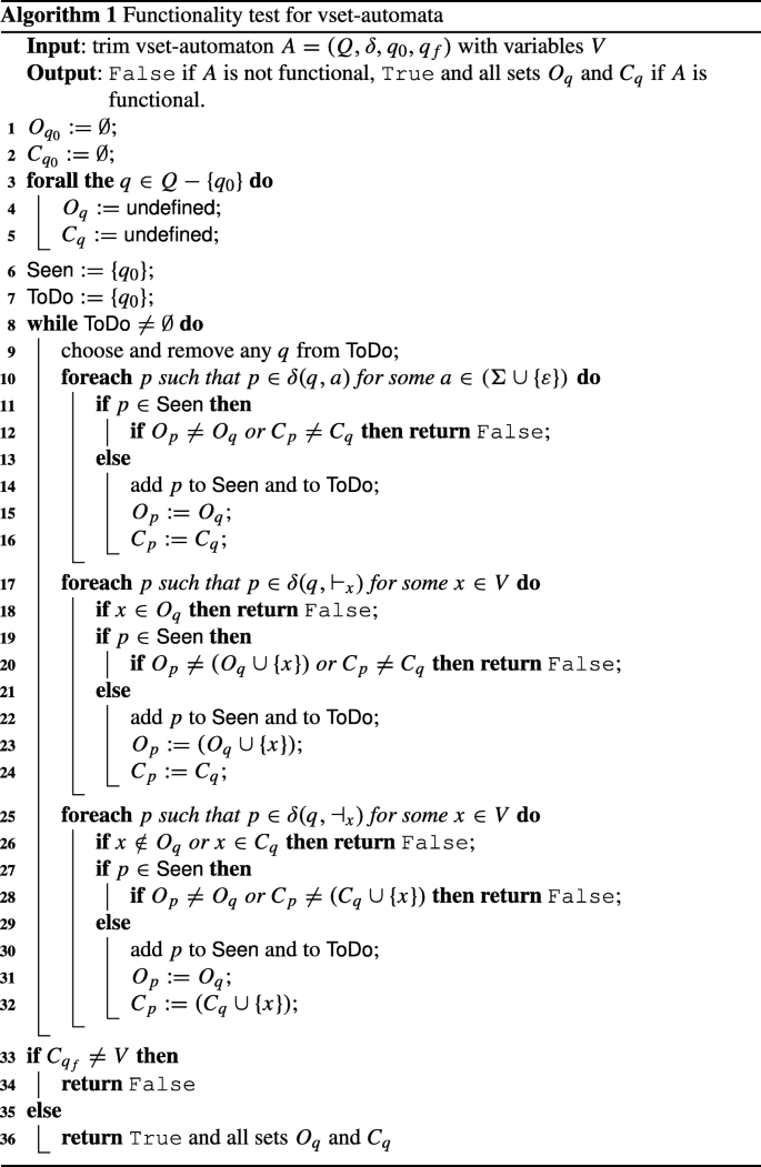
The algorithm tries to find a state q that violates Lemma 3.4. To do so, it inductively constructs all $\phantom {\dot {i}\!}O_{q}$ and all $\phantom {\dot {i}\!}C_{q}$, while looking for a transition that causes these sets to be inconsistent.

We start by defining $\phantom {\dot {i}\!}O_{q_{0}}:= C_{q_{0}}:=\emptyset$, and declaring all sets $\phantom {\dot {i}\!}O_{q}$ and $\phantom {\dot {i}\!}C_{q}$ with $\phantom {\dot {i}\!}q\neq q_{0}$ as undefined. In the main loop, the algorithm picks a state p ∈ Q that has not been picked before and for which $\phantom {\dot {i}\!}O_{p}$ and $\phantom {\dot {i}\!}C_{p}$ are defined. It then iterates over all transitions from p. For each such transition from p to some state q ∈ Q with some label $\phantom {\dot {i}\!}\lambda \in ({\Sigma }\cup {\Gamma }\cup \{\varepsilon \})$, we know that a functional automaton must satisfy the following conditions that depend on $\phantom {\dot {i}\!}\lambda$:

• if $\phantom {\dot {i}\!}\lambda \in ({\Sigma }\cup \{\varepsilon \})$, then $\phantom {\dot {i}\!}O_{q}=O_{p}$ and $\phantom {\dot {i}\!}C_{q}=C_{p}$ must hold,

• if $\phantom {\dot {i}\!}\lambda ={\vdash }_{x}$, then $\phantom {\dot {i}\!}x\notin O_{p}$, $\phantom {\dot {i}\!}O_{q}=O_{p}\cup \{x\}$, and $\phantom {\dot {i}\!}C_{q}=C_{p}$ must hold,

• if $\phantom {\dot {i}\!}\lambda ={\dashv }_{x}$, then $\phantom {\dot {i}\!}x\in O_{p}$, $\phantom {\dot {i}\!}x\notin C_{p}$, $\phantom {\dot {i}\!}O_{q}=O_{p}$, and $\phantom {\dot {i}\!}C_{q}=C_{p}\cup \{x\}$ must hold.

In each case, the conditions describe that the sets for q are correct successors to the sets for p after using this transition. For the variable transitions, the conditions also ensure that each variable is opened or closed only once, and that a variable can only be closed if it has been opened.

If the current transition is a variable transition (i.e., $\phantom {\dot {i}\!}\lambda \in \{{\vdash }_{x},{\dashv }_{x}\}$ for some $\phantom {\dot {i}\!}x\in {\mathsf {SVars}\left (A\right )}$), the algorithm first checks either whether $\phantom {\dot {i}\!}x\notin O_{p}$ (if λ = ⊩_x), or whether $\phantom {\dot {i}\!}x\in O_{p}$ and $\phantom {\dot {i}\!}x\notin C_{p}$ (if $\phantom {\dot {i}\!}\lambda ={\dashv }_{x}$). If this check fails, the algorithm terminates and declares that A is not functional (as q contradicts Lemma 3.4).

If this check succeeds, or if the transition is not a variable transition, the algorithm distinguishes two cases:

• If $\phantom {\dot {i}\!}O_{q}$ and $\phantom {\dot {i}\!}C_{q}$ are undefined, it defines them according to the respective condition and continues.

• If $\phantom {\dot {i}\!}O_{q}$ and $\phantom {\dot {i}\!}C_{q}$ are defined, the algorithm checks whether the sets satisfy the respective condition. If this check fails, the algorithm terminates and declares that A is not functional (like above, we know that q contradicts Lemma 3.4). Otherwise, it continues.

If A has not been declared as not functional, the algorithm then proceeds to the next transition for p (or the next iteration of the main loop).

After the main loop has finished without declaring A as not functional, we know that all transitions of A result in consistent sets $\phantom {\dot {i}\!}O_{q}$ and $\phantom {\dot {i}\!}C_{q}$. Finally, the algorithm declares A to be functional if and only if $\phantom {\dot {i}\!}C_{q_{f}}={\mathsf {SVars}\left (A\right )}$. This is correct for the following reason: If there is an $\phantom {\dot {i}\!}x\in ({\mathsf {SVars}\left (A\right )}- C_{q_{f}})$, we know that $\phantom {\dot {i}\!}|r|_{{\dashv }_{x}}= 0$ for all $\phantom {\dot {i}\!}r\in \mathcal {R}(A)$. Hence, $\phantom {\dot {i}\!}\mathcal {R}$ contains invalid words, which means that A is not functional.

On the other hand, $\phantom {\dot {i}\!}C_{q_{f}}={\mathsf {SVars}\left (A\right )}$ implies $\phantom {\dot {i}\!}O_{q_{f}}={\mathsf {SVars}\left (A\right )}$, as the conditions above ensure that $\phantom {\dot {i}\!}C_{q}\subseteq O_{q}$ for all $\phantom {\dot {i}\!}q\in Q$. Furthermore, the conditions also ensure that each variable is opened and closed exactly once. This allows us to conclude that for all $\phantom {\dot {i}\!}x\in {\mathsf {SVars}\left (A\right )}$, every $\phantom {\dot {i}\!}r\in \mathcal {R}(A)$ contains each of ⊩_x and $\phantom {\dot {i}\!}{\dashv }_{x}$ exactly once, and in the right order. Hence, $\phantom {\dot {i}\!}\mathcal {R}(A)=\mathsf {Ref}(A)$, which means that A is functional, and we can output the sets $\phantom {\dot {i}\!}O_{q}$ and $\phantom {\dot {i}\!}C_{q}$ for all $\phantom {\dot {i}\!}q\in Q$.

All that remains is to verify the upper bound on the running time: The main loop and the included iterations over the transitions touch each of the m transitions exactly once. For each transition, we can perform the checks on the sets in time $\phantom {\dot {i}\!}O(k)$. This yields a total time of $\phantom {\dot {i}\!}O(km)$.

Algorithm for vstk-automata::

This requires only minor modifications: We define $\phantom {\dot {i}\!}N_{q_{0}}:= 0$, and $\phantom {\dot {i}\!}N_{q}$ defaults to undefined for each $\phantom {\dot {i}\!}q\neq q_{0}$. The conditions for transitions from p to q with label $\phantom {\dot {i}\!}\lambda$ are as follows:

• if $\phantom {\dot {i}\!}\lambda \in ({\Sigma }\cup \{\varepsilon \})$, then $\phantom {\dot {i}\!}O_{q}=O_{p}$ and $\phantom {\dot {i}\!}N_{q}=N_{p}$ must hold,

• if $\phantom {\dot {i}\!}\lambda ={\vdash }_{x}$, then $\phantom {\dot {i}\!}x\notin O_{p}$, $\phantom {\dot {i}\!}O_{q}=O_{p}\cup \{x\}$, and $\phantom {\dot {i}\!}N_{q}=N_{p}$ must hold,

• if $\phantom {\dot {i}\!}\lambda ={\dashv }$, then $\phantom {\dot {i}\!}|N_{p}|<|O_{p}|$, $\phantom {\dot {i}\!}O_{q}=O_{p}$, and $\phantom {\dot {i}\!}N_{q}=N_{p}+ 1$ must hold.

The only noteworthy change here is in the last condition: There, we can only process ⊣ if the number of variables that has already been closed is smaller than the number of variables that has been opened. Apart from that, the algorithm proceeds as for vset-automata, with the final check whether $\phantom {\dot {i}\!}|N_{q_{f}}|=|{\mathsf {SVars}\left (A\right )}|$. Analogously to the vset-case, this holds only if $\phantom {\dot {i}\!}O_{q_{f}}={\mathsf {SVars}\left (A\right )}$.

□

Recall that we showed in Lemma 3.1 and Corollary 3.2 suggest that evaluation of v-automata in general is NP-hard. But for functional v-automata, we can use the information that is encoded in the $\phantom {\dot {i}\!}O_{q}$ and $\phantom {\dot {i}\!}C_{q}$ (or $\phantom {\dot {i}\!}O_{q}$ and $\phantom {\dot {i}\!}N_{q}$) for an efficient evaluation algorithm. In other words, non-functionality is the only source of intractability for v-automata evaluation.

Lemma 3.6

Given $\phantom {\dot {i}\!}w\in {\Sigma }^{*}$ , a functional $\phantom {\dot {i}\!}A\in \mathsf {VA}$ , and a $\phantom {\dot {i}\!}({\mathsf {SVars}\left (A\right )},w)$ -tuple μ , we can decide in polynomial time whether $\phantom {\dot {i}\!}\mu \in \llbracket A \rrbracket (w)$ .

Proof

We first show the vset-automata case; the construction for vstk-automata only requires some minor modifications and is given at the end of the proof. Let $\phantom {\dot {i}\!}A=(Q,q_{0},q_{f},\delta )$ be a functional vset-automaton. Now, we need to keep in mind that, for every $\phantom {\dot {i}\!}w\in {\Sigma }^{*}$, multiple ref-words r can define the same $\phantom {\dot {i}\!}({\mathsf {SVars}\left (A\right )},w)$-tuple $\phantom {\dot {i}\!}\mu ^{r}$. For example, if $\phantom {\dot {i}\!}\mu (x)=\mu (y)$, the corresponding ref-word can contain e.g. ⊩_x ⊩_y⊣_x⊣_y or ⊩_y⊣_y⊩_x⊣_x (or any other arrangement that opens and closes each variable in the right order). To deal with this partial commutativity, we represent $\phantom {\dot {i}\!}\mu$ as a sequences of words $\phantom {\dot {i}\!}w_{0},\ldots ,w_{n}\in {\Sigma }^{*}$ and sequence of sets $\phantom {\dot {i}\!}M_{1},\ldots ,M_{n}\subseteq {\Gamma }$ for some $\phantom {\dot {i}\!}n\geq 0$ such that the following holds:

• 1. w = w₀w₁⋯w_n,

• 2. w_i≠ε for 0 < i < n,

• 3. the sets M₁,…,M_n are non-empty and pairwise disjoint,

• 4. $\bigcup _{i = 1}^{n} M_{i} = \{{\vdash }_{x},{\dashv }_{x}\mid x\in {\mathsf {SVars}\left (A\right )}\}$,

• 5. μ(x) = [o,c〉 if and only if there exist 1 ≤ i ≤ j ≤ n with ⊩_x ∈ M_i, ⊣_x ∈ M_j, o = |w₀⋯w_i− 1| + 1, and c = |w₀⋯w_j− 1| + 1.

Intuitively, the combined sequence $\phantom {\dot {i}\!}w_{0},M_{1},w_{1},\dots ,M_{n},w_{n}$ describes how A has to match $\phantom {\dot {i}\!}\mu$ to w, where successive variable transitions are considered commutative. The words $\phantom {\dot {i}\!}w_{i}$ describe the how A consumes the input, and the sets $\phantom {\dot {i}\!}M_{i}$ describe how A acts on variables. Hence, the sequence captures how A alternates between both types of behavior.

As a consequence, if $\phantom {\dot {i}\!}r\in ({\Sigma }\cup {\Gamma })^{*}$ with $\phantom {\dot {i}\!}\mu ^{r}=\mu$, then for every $\phantom {\dot {i}\!}M_{i}$, the symbols in $\phantom {\dot {i}\!}M_{i}$ can be arranged into a word $\phantom {\dot {i}\!}v_{i}\in {\Gamma }^{+}$ such that r = w₀(v₁w₁)⋯(v_nw_n). As we require $\phantom {\dot {i}\!}w_{i}\neq \varepsilon$ and $\phantom {\dot {i}\!}S_{i}\neq \emptyset$, every pair $\phantom {\dot {i}\!}\mu$ and w defines a unique pair of sequences w₀,…,w_n and $\phantom {\dot {i}\!}M_{1},\ldots ,M_{\ell }$.

We now simulate all possible r with $\phantom {\dot {i}\!}\mu ^{r}=\mu$ using a generalization of the on-the-fly computation of the powerset construction (for the simulation of NFAs with DFAs). More specifically, the algorithm shall construct a sequence of sets $\phantom {\dot {i}\!}S_{0},T_{1},S_{1},\dots ,T_{n},S_{n}\subseteq Q$, where each $\phantom {\dot {i}\!}S_{i}$ describes the states that A can have after processing $\phantom {\dot {i}\!}w_{0}, (M_{1}, w_{1}),\dots ,(M_{i}, w_{i})$, while $\phantom {\dot {i}\!}T_{i}$ describes the states that can be reached by processing $\phantom {\dot {i}\!}(w_{0}, M_{1}), \dots , (w_{i-1}, M_{i})$.

In order to ensure that the $\phantom {\dot {i}\!}T_{i}$ are computed correctly, we also define

$$O_{i} := \bigcup_{j = 1}^{i} \{x \mid {\vdash}_{x}\in M_{j}\}, \quad C_{i} := \bigcup_{j = 1}^{i} \{x\mid {\dashv}_{x}\in M_{j}\} $$

for all $\phantom {\dot {i}\!}1\leq i\leq \ell$, as well as $\phantom {\dot {i}\!}O_{0}:= C_{0} := \emptyset$. Intuitively, $\phantom {\dot {i}\!}O_{i}$ and $\phantom {\dot {i}\!}C_{i}$ shall represent the sets $\phantom {\dot {i}\!}O_{q}$ and $\phantom {\dot {i}\!}C_{q}$ for any q that can be reached after processing $\phantom {\dot {i}\!}w_{0} (M_{1} w_{1})\cdots (M_{i} w_{i})$. This necessarily results in $\phantom {\dot {i}\!}O_{n}=C_{n}={\mathsf {SVars}\left (A\right )}$.

We now define $\phantom {\dot {i}\!}S_{0} := \delta ^*(q_{0},w_{0})$. The algorithm then iterates the following loop for i from 1 to n:

• 1. Let T_i be the set of all states q ∈ Q such that

  • (a) O_q = O_i and C_q = C_i, and

  • (b) there exists a state p ∈ S_i− 1 such that q can be reached from p using only ε-transitions and variable-transitions.

• 2. Let $S_{i}:= \bigcup _{p\in T_{i}} \delta ^*(p,w_{i})$.

After computing $\phantom {\dot {i}\!}S_{n}$, we only need to check whether $\phantom {\dot {i}\!}q_{f}\in S_{n}$. This holds if and only if there is an $\phantom {\dot {i}\!}r\in \mathcal {R}(A)$ with $\phantom {\dot {i}\!}\mu ^{r}=\mu$. Hence, we can decide μ ∈⟦A⟧(w); and this is clearly possible in polynomial time (recall that due to Lemma 3.5, we can precompute the sets $\phantom {\dot {i}\!}O_{q}$ and $\phantom {\dot {i}\!}C_{q}$ for all $\phantom {\dot {i}\!}q\in Q$ in polynomial time).

vstk-automata: :

For vstk-automata, instead of storing different $\phantom {\dot {i}\!}{\dashv }_{x}$ in the sets $\phantom {\dot {i}\!}M_{i}$, and using these to compute $\phantom {\dot {i}\!}C_{i}$ for every step i, we compute sets $\phantom {\dot {i}\!}N_{i}$ that determine how many variables have been closed.

We also have to refine the computation of the $\phantom {\dot {i}\!}T_{i}$ to account for a special case of opening variables: Due to the stack behavior, we can encounter cases where two variables are opened in the same $\phantom {\dot {i}\!}M_{i}$, but closed at different times. Those variables are not commutative within $\phantom {\dot {i}\!}M_{i}$. Hence, we define the partial order $\phantom {\dot {i}\!}\prec _{\mu }$ on $\phantom {\dot {i}\!}{\mathsf {SVars}\left (A\right )}$ such that x ≺_μy if $\phantom {\dot {i}\!}\mu (x)=[k,m\rangle$ and $\phantom {\dot {i}\!}\mu (y)=[k,n\rangle$ with $\phantom {\dot {i}\!}m<n$. In addition to the criteria that hold for vset-automata, the reachability analysis that computes $\phantom {\dot {i}\!}T_{i}$ now may only use transitions from some state $\phantom {\dot {i}\!}p^{\prime }$ to some state $\phantom {\dot {i}\!}q^{\prime }$ with label ⊩_y if $\phantom {\dot {i}\!}x\in O_{p^{\prime }}$ for all $\phantom {\dot {i}\!}x\prec _{\mu } y$.

Apart from that, we proceed analogously to the vset-construction by processing the $\phantom {\dot {i}\!}w_{i}$ as in the simulation of an NFA, and the sets $\phantom {\dot {i}\!}M_{i}$ with a reachability analysis, where the sets $\phantom {\dot {i}\!}O_{i}$ and $\phantom {\dot {i}\!}N_{i}$ determine which states are viable destinations. Clearly, $\phantom {\dot {i}\!}\prec _{\mu }$ can be computed in polynomial time from $\phantom {\dot {i}\!}\mu$. □

This approach was used by Freydenberger, Kimelfeld, and Peterfreund [17] to develop a polynomial delay algorithm for regular spanners.

3.2 Relative Succinctness of v-Automata

Our next goal is to compare the succinctness of functional and general v-automata, as well as that of vstk- and vset-automata. To this end, we introduce a lemma that allows us to treat certain v-automata as NFAs that accept ref-words. Note that the result applies regardless of whether the ref-words close variables by name with ⊣_x or by stack with ⊣. But as a convention, we shall only apply the following lemma to two ref-words if either both of them close variables by name or both of them close variables by stack.

Lemma 3.7

For a finite $\phantom {\dot {i}\!}V\subset {\Xi }$ , consider any valid $\phantom {\dot {i}\!}r\in ({\Sigma }\cup {\Gamma }_{V})^{*}$ that contains no subword from $\phantom {\dot {i}\!}{\Gamma }v^{2}$ . Then for every valid $\phantom {\dot {i}\!}\hat {r}\in ({\Sigma }\cup {\Gamma }v)^{*}$ with $\phantom {\dot {i}\!}\mathsf {clr}(\hat {r})=\mathsf {clr}(r)$ that closes variables in the same way as r, we have that $\phantom {\dot {i}\!}\mu ^{\hat {r}}=\mu ^{r}$ implies $\phantom {\dot {i}\!}\hat {r}=r$ .

Proof

Every valid $\phantom {\dot {i}\!}r\in ({\Sigma }\cup {\Gamma }_{V})^{*}$ that contains no subword from $\phantom {\dot {i}\!}{\Gamma }v^{2}$ has a unique factorization $\phantom {\dot {i}\!}r = w_{0} (v_{1} w_{1}){\cdots } (v_{2k}w_{2k})$ with $\phantom {\dot {i}\!}v_{i}\in {\Gamma }v$, $\phantom {\dot {i}\!}w_{0},w_{2k}\in {\Sigma }^{*}$, and $\phantom {\dot {i}\!}w_{1},\ldots ,w_{2k-1}\in {\Sigma }^{+}$. Hence, for all $\phantom {\dot {i}\!}x\in V$ and $\phantom {\dot {i}\!}[i_{x},j_{x}\rangle :=\mu ^{r}(x)$, we have $\phantom {\dot {i}\!}i_{x}\neq j_{x}$; and for all $\phantom {\dot {i}\!}y\in (V-\{x\})$ and $\phantom {\dot {i}\!}[i_{y},j_{y}\rangle := \mu ^{r}(y)$, we know $\phantom {\dot {i}\!}i_{x},j_{x},i_{y},j_{y}$ are pairwise distinct.

Now assume that there is a valid $\phantom {\dot {i}\!}\hat {r}\in ({\Sigma }\cup {\Gamma }v)^{*}$ with $\phantom {\dot {i}\!}\mathsf {clr}(\hat {r})=\mathsf {clr}(r)$ and $\phantom {\dot {i}\!}\mu ^{\hat {r}}=\mu ^{r}$. We first observe that $\phantom {\dot {i}\!}\hat {r}$ contains no factor from $\phantom {\dot {i}\!}{\Gamma }v^{2}$. Otherwise, we would have $\phantom {\dot {i}\!}\mu ^{\hat {r}}\neq \mu ^{r}$, as there would be some $\phantom {\dot {i}\!}x\in V$ where $\phantom {\dot {i}\!}i_{\hat {x}} = j_{\hat {x}}$ for $[i_{\hat {x}},j_{\hat {x}}\rangle :=\mu ^{\hat {r}}(x)$, or there is some $\phantom {\dot {i}\!}y\in (V-\{x\})$ such that $\phantom {\dot {i}\!}i_{\hat {x}},j_{\hat {x}},i_{\hat {y}},j_{\hat {y}}$ are not pairwise distinct for $[i_{\hat {y}},j_{\hat {y}}\rangle :=\mu ^{\hat {r}}(y)$.

Thus, $\phantom {\dot {i}\!}\hat {r}$ can be factorized into $\phantom {\dot {i}\!}\hat {r} = \hat {w}_{0} (\hat {v}_{1} \hat {w}_{1}){\cdots } (\hat {v}_{2k}\hat {w}_{2k})$, analogously to r. By comparing the factorizations of r and $\phantom {\dot {i}\!}\hat {r}$ from left to right, we observe that $\phantom {\dot {i}\!}\hat {w}_{i} = w_{i}$ and $\phantom {\dot {i}\!}\hat {v}_{j}=v_{j}$ has to hold for all i and j. Otherwise, we would obtain a contradiction to $\mu ^{\hat {r}}=\mu ^{r}$ or $\phantom {\dot {i}\!}\mathsf {clr}(\hat {r})=\mathsf {clr}(r)$. We conclude $\phantom {\dot {i}\!}\hat {r}=r$. □

Lemma 3.7 provides us with a sufficient criterion for ref-words r that uniquely define μ^r. This allows us to identify v-automata that can be treated as NFAs. In particular, we shall use the following result by Birget [4] (although the proof in [4] refers only to NFAs without $\phantom {\dot {i}\!}\varepsilon$-transitions, it directly generalizes to those with $\phantom {\dot {i}\!}\varepsilon$-transitions).

Lemma 3.8 (Birget 4)

Let L be a regular language. Assume there exist pairs of words $\phantom {\dot {i}\!}(u_{1}, v_{1}), {\ldots } , (u_{n}, v_{n})$ such that

• 1. u_iv_i ∈ Lfor1 ≤ i ≤ n,and

• 2. u_iv_j∉Loru_jv_i∉Lforall 1 ≤ i < j ≤ n.

Then any NFA accepting L must have at least n states.

Now we are ready to compare functional and general v-automaton. The author considers it no surprise that standard automata techniques allow us to transform every vset- or vstk-automaton into an equivalent functional v-automaton of the same type; but this may result in an exponential number of states. While combining Lemma 3.1 with Lemma 3.6 already suggests that this conversion is not possible in polynomial time (unless the number of variables is bounded, or $\phantom {\dot {i}\!}\mathsf {P}=\mathsf {NP}$), we also show matching exponential size bounds.

Proposition 3.9

Let $\phantom {\dot {i}\!}f_{\mathsf {set}}(k):= 3^{k}$, $\phantom {\dot {i}\!}f_{\mathsf {stk}}(k):= (k + 2)2^{k-1}$,and $\phantom {\dot {i}\!}s\in \{\mathsf {set},\mathsf {stk}\}$.For every $\phantom {\dot {i}\!}A\in \mathsf {VA}_{s}$with nstates andk variables, there exists an equivalent functionalA_fun ∈VA_swith $\phantom {\dot {i}\!}n\cdot f_{s}(k)$states.For every $\phantom {\dot {i}\!}k\geq 1$,there is an $\phantom {\dot {i}\!}A_{k}\in \mathsf {VA}_{s}$withone state andk variables, such that every equivalent functionalA_fun ∈VA_shasat least $\phantom {\dot {i}\!}f_{s}(k)$states.

Proof

This proof is organized as follows: We first discuss vset-automata, then vstk-automata. For each of these, we first discuss upper and then lower bounds.

Upper bound for vset-automata::

Consider a vset-automaton $\phantom {\dot {i}\!}A=(Q,q_{0},q_{f},\delta )$ with $\phantom {\dot {i}\!}k\geq 1$ variables. Our goal is to construct a functional vset-automaton $\phantom {\dot {i}\!}A_{\mathsf {fun}}$ with $\phantom {\dot {i}\!}3^{k}|Q|$ states and $\phantom {\dot {i}\!}\llbracket {A_{\mathsf {fun}}}\rrbracket =\llbracket {A}\rrbracket$. The main idea is to intersect A with a functional vset-automaton that keeps track of the sets $\phantom {\dot {i}\!}O_{q}$ and $\phantom {\dot {i}\!}C_{q}$ for all $\phantom {\dot {i}\!}q\in Q$ (Definition 3.3). Formally, we associate each state of $\phantom {\dot {i}\!}A_{\mathsf {fun}}$ with a function $\phantom {\dot {i}\!}s\colon \mathsf {SVars}({A})\to \{\mathtt {w},\mathtt {o},\mathtt {c}\}$, where $\phantom {\dot {i}\!}s(x)$ represents the following:

• $\phantom {\dot {i}\!}\mathtt {w}$ stands for “waiting”, meaning ⊩_x has not been read,

• $\phantom {\dot {i}\!}\mathtt {o}$ stands for “open”, meaning ⊩_x has been read, but not $\phantom {\dot {i}\!}{\dashv }_{x}$,

• $\phantom {\dot {i}\!}\mathtt {c}$ stands for “closed”, meaning ⊩_x and $\phantom {\dot {i}\!}{\dashv }_{x}$ have been read.

Let S be the set of all such functions. Observe that $\phantom {\dot {i}\!}|S|= 3^{k}$. We now define $\phantom {\dot {i}\!}A_{\mathsf {fun}}:= (Q_{\mathsf {fun}},q_{0}^{\mathsf {fun}},q_{f}^{\mathsf {fun}},\delta _{\mathsf {fun}})$ in the following way:

• $\phantom {\dot {i}\!}Q_{\mathsf {fun}}:= Q\times S$,

• $\phantom {\dot {i}\!}q_{0}^{\mathsf {fun}}:= (q_{0},s_{0})$, where $\phantom {\dot {i}\!}s_{0}$ is defined by $\phantom {\dot {i}\!}s_{0}(x) = \mathtt {w}$ for all $\phantom {\dot {i}\!}x\in {\mathsf {SVars}\left (A\right )}$,

• $\phantom {\dot {i}\!}q_{f}^{\mathsf {fun}}:= (q_{f},s_{f})$, where $\phantom {\dot {i}\!}s_{f}$ is defined by $\phantom {\dot {i}\!}s_{f}(x)=\mathtt {c}$ for all $\phantom {\dot {i}\!}x\in {\mathsf {SVars}\left (A\right )}$,

• $\phantom {\dot {i}\!}\delta _{\mathsf {fun}}((p,s),a):= \{(q,s)\mid q\in \delta (p,a)\}$ for $\phantom {\dot {i}\!}a\in ({\Sigma }\cup \{\varepsilon \})$ and $\phantom {\dot {i}\!}(p,s)\in Q_{\mathsf {fun}}$,

• for all $\phantom {\dot {i}\!}(p,s)\in Q_{\mathsf {fun}}$ and all $\phantom {\dot {i}\!}x\in {\mathsf {SVars}\left (A\right )}$, let

  $$\begin{array}{@{}rcl@{}} \delta_{\mathsf{fun}}((p,s),{\vdash}_{x})&:=& \left\{\begin{array}{ll} \emptyset & \text{if } s(x)\neq\mathtt{w},\\ \{(q,t_{o})\mid q\in\delta(p,{\vdash}_{x})\} & \text{if } s(x)=\mathtt{w}, \end{array}\right.\\ \delta_{\mathsf{fun}}((p,s),{\dashv}_{x})&:=& \left\{\begin{array}{ll} \emptyset & \text{if } s(x)\neq\mathtt{o},\\ \{(q,t_{c})\mid q\in\delta(p,{\dashv}_{x})\} & \text{if } s(x)=\mathtt{o}, \end{array}\right. \end{array} $$

  where $\phantom {\dot {i}\!}t_{o}$ is defined by $\phantom {\dot {i}\!}t(x):= \mathtt {o}$ and $\phantom {\dot {i}\!}t_{o}(y):= s(y)$ for all $\phantom {\dot {i}\!}y\neq x$, and $\phantom {\dot {i}\!}t_{c}$ is defined by $\phantom {\dot {i}\!}t_{c}(x):= \mathtt {c}$ and $\phantom {\dot {i}\!}t_{c}(y):= s(y)$ for all $\phantom {\dot {i}\!}y\neq x$.

In order to see that $\phantom {\dot {i}\!}A_{\mathsf {fun}}$ is correct and functional, note that it simulates A, while the definition of $\phantom {\dot {i}\!}\delta _{\mathsf {fun}}$ ensures that in each state $\phantom {\dot {i}\!}(q,s)$, each variable x can only be opened if $\phantom {\dot {i}\!}s(x)=\mathtt {w}$, and only be closed if $\phantom {\dot {i}\!}s(x)=\mathtt {o}$. The initial state $\phantom {\dot {i}\!}(q_{0},s_{0})$ and the final state $\phantom {\dot {i}\!}(q_{f},s_{f})$ ensure that every variable is opened and closed exactly once. Finally, as $\phantom {\dot {i}\!}A_{\mathsf {fun}}$ has exactly $\phantom {\dot {i}\!}3^{k} |Q|$ states, this proves the upper bound for vset-automata.

Lower bound for vset-automata::

Let $\phantom {\dot {i}\!}\mathtt {a}\in {\Sigma }$, $\phantom {\dot {i}\!}k\geq 1$, and $\phantom {\dot {i}\!}X_{k}:=\{x_{1},\ldots ,x_{k}\}\subset {\Xi }$. We define the following vset-automaton $\phantom {\dot {i}\!}A_{k}$ with variables $\phantom {\dot {i}\!}X_{k}$:

In the terminology of [13], $\phantom {\dot {i}\!}A_k$ defines the universal spanner over $\phantom {\dot {i}\!}\{\mathtt {a}\}$ with variables $\phantom {\dot {i}\!}X_k$.

Recall the set S of all functions $\phantom {\dot {i}\!}s\colon X_k\to \{\mathtt {w},\mathtt {o},\mathtt {c}\}$, which we already used for the upper bound above. For every $\phantom {\dot {i}\!}s\in S$, we define ref-words $u_s:= u^s_1{\cdots } u^s_k$ and $\phantom {\dot {i}\!}v_s:= v^s_1 {\cdots } v^s_k$, where the words $\phantom {\dot {i}\!}u^s_i$ and $\phantom {\dot {i}\!}v^s_i$ are defined as follows for every i, $\phantom {\dot {i}\!}1\leq i\leq k$:

$$\begin{array}{@{}rcl@{}} {u^{s}_{i}}&:=& \left\{\begin{array}{ll} \varepsilon & \text{if } s(x_{i}) = \mathtt{w},\\ {\vdash}_{x_{i}}\mathtt{a} & \text{if } s(x_{i}) = \mathtt{o},\\ {\vdash}_{x_{i}}\mathtt{a}{\dashv}_{x_{i}}\mathtt{a} & \text{if } s(x_{i}) = \mathtt{c} \end{array}\right.\\ {v^{s}_{i}}&:=& \left\{\begin{array}{ll} {\vdash}_{x_{i}}\mathtt{a}{\dashv}_{x_{i}}\mathtt{a} & \text{if } s(x_{i}) = \mathtt{w},\\ {\dashv}_{x_{i}}\mathtt{a} & \text{if } s(x_{i}) = \mathtt{o},\\ \varepsilon& \text{if } s(x_{i}) = \mathtt{c} \end{array}\right. \end{array} $$

Now observe that $\phantom {\dot {i}\!}u_s\cdot v_s\in \mathsf {Ref}(A_k)$ for each $\phantom {\dot {i}\!}s\in S$. Furthermore, $\phantom {\dot {i}\!}u_s\cdot v_s$ does not contain any subword from $\phantom {\dot {i}\!}{\Gamma }^2$. Hence, according to Lemma 3.7, $\phantom {\dot {i}\!}u_s v_s\in \mathsf {Ref}(A)$ must hold for every vset-automaton A with $\phantom {\dot {i}\!}\llbracket A \rrbracket =\llbracket A_k \rrbracket$.

Let $\phantom {\dot {i}\!}A\in \mathsf {\mathsf {VA}_{\mathsf {set}}}$ be functional with $\phantom {\dot {i}\!}\llbracket A \rrbracket =\llbracket A_k \rrbracket$. As A is functional, $\phantom {\dot {i}\!}\mathsf {Ref}(A)=\mathcal {R}(A)$, which implies $\phantom {\dot {i}\!}u_s\cdot v_s\in \mathcal {R}(A)$ for all $\phantom {\dot {i}\!}s\in S$. Furthermore, for all $\phantom {\dot {i}\!}s,t\in S$ with $\phantom {\dot {i}\!}s\neq t$, we have that $\phantom {\dot {i}\!}u_s\cdot v_t \notin \mathcal {R}(A)$ must hold, as $\phantom {\dot {i}\!}u_s\cdot v_t$ is not a valid ref-word. In order to see this, consider an $\phantom {\dot {i}\!}x_i$ with s(x_i)≠t(x_i). As each ${\vdash }_{x_i}$ and $\phantom {\dot {i}\!}{\dashv }_{x_i}$ occurs only in $\phantom {\dot {i}\!}u^s_i$ and $\phantom {\dot {i}\!}v^t_i$, the ref-word $\phantom {\dot {i}\!}u_s\cdot v_t$ cannot contain both of ${\vdash }_{x_i}$ and $\phantom {\dot {i}\!}{\dashv }_{x_i}$ exactly once.

This allows us to use Lemma 3.8: For each $\phantom {\dot {i}\!}s\in S$, we observe $\phantom {\dot {i}\!}u_s\cdot v_s \in \mathcal {R}(A)$ and $\phantom {\dot {i}\!}u_s \cdot v_t \notin \mathcal {R}(A)$ for all $\phantom {\dot {i}\!}t\in S$ with $\phantom {\dot {i}\!}t\neq s$. Hence, A has at least $\phantom {\dot {i}\!}|S|= 3^k$ states. As A was chosen freely among functional vset-automata, this proves the claimed lower bound.

Upper bound for vstk-automata: :

Assume $\phantom {\dot {i}\!}A=(Q,q_0,q_f,\delta )$ is a vstk-automaton with $\phantom {\dot {i}\!}k\geq 1$ variables. Our goal is to construct a functional vstk-automaton $\phantom {\dot {i}\!}A_{\mathsf {fun}}$ with $\phantom {\dot {i}\!}(k + 2)2^{k-1}|Q|$ states and $\phantom {\dot {i}\!}\llbracket {A_{\mathsf {fun}}}\rrbracket =\llbracket {A}\rrbracket$. On a conceptual level, the construction is very similar to the vset-automata construction above. The only difference is what information on the variables is stored in the states. For vstk-automata, we store which variables have been opened (to ensure that every variable is opened exactly once), and how many variables have been closed (to ensure that every variable is closed at least once, and to prevent processing $\phantom {\dot {i}\!}{\dashv }$ when no variables can be closed). We now define $\phantom {\dot {i}\!}A_{\mathsf {fun}}:= (Q_{\mathsf {fun}},q_{0}^{\mathsf {fun}},q_{f}^{\mathsf {fun}},\delta _{\mathsf {fun}})$ in the following way:

• $\phantom {\dot {i}\!}Q_{\mathsf {fun}}:= \{ (q, O, i) \mid q\in Q, O\subseteq {\mathsf {SVars}\left (A\right )}, 0\leq i \leq |O|\}$,

• $\phantom {\dot {i}\!}q_{0}^{\mathsf {fun}}:= (q_0,\emptyset ,0)$,

• $\phantom {\dot {i}\!}q_{f}^{\mathsf {fun}}:= (q_f,{\mathsf {SVars}\left (A\right )},k)$,

• $\phantom {\dot {i}\!}\delta _{\mathsf {fun}}((p,O,i),a):= \{(q,O,i)\mid q\in \delta (p,a)\}$ for $\phantom {\dot {i}\!}a\in ({\Sigma }\cup \{\varepsilon \})$ and $\phantom {\dot {i}\!}(p,O,i)\in Q_{\mathsf {fun}}$,

• for all $\phantom {\dot {i}\!}(p,O,i)\in Q_{\mathsf {fun}}$ and all $\phantom {\dot {i}\!}x\in {\mathsf {SVars}\left (A\right )}$, let

  $$\begin{array}{@{}rcl@{}} \delta_{\mathsf{fun}}((p,O,i),{\vdash}_{x})&:=& \left\{\begin{array}{ll} \emptyset & \text{if } x\in O,\\ \{(q,O\cup\{x\},i)\mid q\in\delta(p,{\vdash}_{x})\} & \text{if } x\notin O, \end{array}\right.\\ \delta_{\mathsf{fun}}((p,O,i),{\dashv})&:=& \left\{\begin{array}{ll} \emptyset & \text{if } i\geq |O|,\\ \{(q,O,i + 1)\mid q\in\delta(p,{\dashv})\} & \text{if } i< |O| \end{array}\right. \end{array} $$

It is now easy to see that $\phantom {\dot {i}\!}A_{\mathsf {fun}}$ simulates A. In addition to this, the definition of $\phantom {\dot {i}\!}\delta _{\mathsf {fun}}$ ensures that variables are only opened if they have not been opened before (as ⊩_x can only be precessed if $\phantom {\dot {i}\!}x\notin O$), and that variables can only be closed if there are sufficiently many open variables (as $\phantom {\dot {i}\!}{\dashv }$ can only be processed if i < |O|). Furthermore, $\phantom {\dot {i}\!}A_{\mathsf {fun}}$ accepts only if every variable has been opened, and if k variables have been closed. Hence, $\phantom {\dot {i}\!}A_{\mathsf {fun}}$ is functional and equivalent to A. All that remains for this upper bound is to prove that $\phantom {\dot {i}\!}|Q_{\mathsf {fun}}| = (k + 2)2^{k-1}|Q|$. First, note that in the definition of $\phantom {\dot {i}\!}Q_{\mathsf {fun}}$, each state of Q is paired with an element of the set $\phantom {\dot {i}\!}M := \{(O,i) \mid O\subseteq {\mathsf {SVars}\left (A\right )}, 0\leq i\leq |O|\}$. We observe that $\phantom {\dot {i}\!}|M| = {\sum }_{j = 0}^{k} \binom {k}{j} (j + 1)$, as there are $\phantom {\dot {i}\!}\binom {k}{j}$ possible sets O with $\phantom {\dot {i}\!}|O|=j$; and for each such set, we have $\phantom {\dot {i}\!}(j + 1)$ choices for i. By simplifying this formula (e.g. using ones favorite software), we obtain $\phantom {\dot {i}\!}|M|=(k + 2)2^{k-1}$. As |Q_fun| = |M||Q|, this concludes the proof of the upper bound.

Lower bound for vstk-automata: :

Again, this proof is similar to the vstk-case. Let $\phantom {\dot {i}\!}\mathtt {a}\in {\Sigma }$, $\phantom {\dot {i}\!}k\geq 1$, and $\phantom {\dot {i}\!}X_k:=\{x_1,\ldots ,x_k\}\subset {\Xi }$. We define the following vset-automaton $\phantom {\dot {i}\!}A_k$ with variables $\phantom {\dot {i}\!}X_k$:

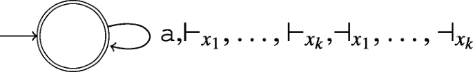
In the terminology of [13], $\phantom {\dot {i}\!}A_{k}$ defines the universal hierarchical spanner over $\phantom {\dot {i}\!}\{\mathtt {a}\}$ with variables $\phantom {\dot {i}\!}X_{k}$. Again, we want to define a sequence of pairs of ref-words that allows us to use Lemma 3.8. Recall the set $\phantom {\dot {i}\!}M := \{(O,i) \mid O\subseteq X_{k}, i\leq |O|\}$ that we already used in the proof for the upper bound. For each $\phantom {\dot {i}\!}(O,i)\in M$, we define ref-words $\phantom {\dot {i}\!}u_{O,i} := {u^{O}_{1}}{\cdots } {u^{O}_{k}} ({\dashv } \mathtt {a})^{i}$ and $\phantom {\dot {i}\!}v_{O,i}:= {v^{O}_{1}}{\cdots } {v^{O}_{k}} ({\dashv } \mathtt {a})^{k-i}$ by

$$\begin{array}{@{}rcl@{}} {u^{O}_{j}} &:=& \left\{\begin{array}{ll} {\vdash}_{x_{j}}\mathtt{a} & \text{if } x_{j}\in O,\\ \varepsilon & \text{if } x_{j}\notin O \end{array}\right.\\ {v^{O}_{j}} &:=& \left\{\begin{array}{ll} \varepsilon & \text{if } x_{j}\in O,\\ {\vdash}_{x_{j}}\mathtt{a} & \text{if } x_{j}\notin O \end{array}\right. \end{array} $$

for all j with $\phantom {\dot {i}\!}1\leq j\leq k$. First, observe that $\phantom {\dot {i}\!}u_{O,i}\cdot v_{O,i}\in \mathsf {Ref}(A_{k})$ holds for all $\phantom {\dot {i}\!}(O,i)\in M$. Assume that A is a functional vstk-automaton with ⟦A⟧ = ⟦A_k⟧. As Lemma 3.7 applies, we know that $\phantom {\dot {i}\!}u_{O,i}\cdot v_{O,i}\in \mathcal {R}(A)$ holds for all $\phantom {\dot {i}\!}(O,i)\in M$. Next, consider $(O,i), (O^{\prime },i^{\prime })\in M$ with $\phantom {\dot {i}\!}(O,i)\neq (O^{\prime },i^{\prime })$ and let $\phantom {\dot {i}\!}r:= u_{O,i}\cdot v_{O^{\prime },i^{\prime }}$. Then $\phantom {\dot {i}\!}r\notin \mathcal {R}(A)$ must hold: If $\phantom {\dot {i}\!}i\neq i^{\prime }$, then r contains too many or too few occurrences of $\phantom {\dot {i}\!}{\dashv }$. If $\phantom {\dot {i}\!}O\neq O^{\prime }$, then a variable x is opened more than once (if $\phantom {\dot {i}\!}x\in O$ and $\phantom {\dot {i}\!}x\notin O^{\prime }$) or less than once (if $\phantom {\dot {i}\!}x\notin O$ and $\phantom {\dot {i}\!}x\in O^{\prime }$). In each of these cases, r is not valid, which contradicts our assumption that A is functional. Hence, we can apply Lemma 3.8, and conclude that A has at least $\phantom {\dot {i}\!}|M|$ states. As we established in the proof of the upper bound, $\phantom {\dot {i}\!}|M|=(k + 2)2^{k-1}$.

□

We also briefly compare vset- and vstk-automata: It was shown in [13] that $\phantom {\dot {i}\!}\llbracket \mathsf {\mathsf {VA}_{\mathsf {stk}}} \rrbracket \subset \llbracket \mathsf {\mathsf {VA}_{\mathsf {set}}} \rrbracket$. This inclusion is proper for the following reason: As vstk-automata always close the variable that was opened most recently, they can only express hierarchical spanners (a spanner is hierarchical if it contains only w-tuples with non-overlapping spans; for a formal definition, see [13]). While this behavior can be simulated with vset-automata, a slight modification of the proof of Proposition 3.9 shows that this causes an exponential blowup.

Proposition 3.10

For every $\phantom {\dot {i}\!}k\geq 1$ , there is a vstk-automaton $\phantom {\dot {i}\!}A_{k}$ with one state and k variables, such that every vset-automaton A with $\phantom {\dot {i}\!}\llbracket A \rrbracket =\llbracket A_{k} \rrbracket$ has at least $\phantom {\dot {i}\!}k!$ states.

Proof

Let $\phantom {\dot {i}\!}\mathtt {a}\in {\Sigma }$, $\phantom {\dot {i}\!}k\geq 1$, and $\phantom {\dot {i}\!}X_{k}:=\{x_{1},\ldots ,x_{k}\}\subset {\Xi }$. We use the same vstk-automaton $\phantom {\dot {i}\!}A_{k}$ as in the proof of the lower bound for vstk-automata in Proposition 3.9.

We now focus on the following subset of $\phantom {\dot {i}\!}\mathsf {Ref}(A_{k})$:

$$R_{k}:= \left\{ ({\vdash}_{x_{p(1)}} \mathtt{a}) {\cdots} ({\vdash}_{x_{p(k)}} \mathtt{a}) ({\dashv} \mathtt{a})^{k} \mid p\in\mathsf{Perm}(k)\right\}, $$

where $\phantom {\dot {i}\!}\mathsf {Perm}(k)$ is the set of all permutations of $\phantom {\dot {i}\!}\{1,\ldots ,k\}$. Translating these ref-words to ref-words that use explicit closing commands, we obtain the language

$$R^{\prime}_{k}:= \left\{ ({\vdash}_{x_{p(1)}} \mathtt{a}) {\cdots} ({\vdash}_{x_{p(k)}} \mathtt{a}) ({\dashv}_{x_{p(k)}} \mathtt{a}) {\cdots} ({\dashv}_{x_{p(1)}} \mathtt{a}) \mid p\in\mathsf{Perm}(k)\right\}.$$

As $\phantom {\dot {i}\!}R^{\prime }_{k}$ makes the closing of variables explicit, we can state that for every $\phantom {\dot {i}\!}r\in R_{k}$, there is an $\phantom {\dot {i}\!}r^{\prime }\in R^{\prime }_{k}$ with $\phantom {\dot {i}\!}\mu ^{r} = \mu ^{r^{\prime }}$, and vice versa. Hence, for every vset-automaton A with $\phantom {\dot {i}\!}\llbracket {A}\rrbracket =\llbracket {A_{k}\rrbracket }$, Lemma 3.7 implies that $\phantom {\dot {i}\!}R^{\prime }_{k}\subseteq \mathcal {R}(A)$. For every permutation p ∈Perm(k), we now define

$$u_{p}:= ({\vdash}_{x_{p(1)}}\mathtt{a}){\cdots} ({\vdash}_{x_{p(k)}}\mathtt{a}), \quad v_{p} := ({\dashv}_{x_{p(k)}}\mathtt{a}){\cdots} ({\dashv}_{x_{p(1)}}\mathtt{a}). $$

Then $\phantom {\dot {i}\!}u_{p}v_{p}\in R^{\prime }_{k}$ holds for every $\phantom {\dot {i}\!}p\in \mathsf {Perm}(k)$, which implies $\phantom {\dot {i}\!}u_{p}v_{p}\in \mathcal {R}(A)$. Next, consider any $\phantom {\dot {i}\!}p,q\in \mathsf {Perm}(k)$ with $\phantom {\dot {i}\!}p\neq q$, and let r := u_pv_q. Choose the largest i for which $\phantom {\dot {i}\!}p(i)\neq q(i)$. As $\phantom {\dot {i}\!}p(j)=q(j)$ for all $\phantom {\dot {i}\!}j>i$, the ref-words $\phantom {\dot {i}\!}v_{p}$ and $\phantom {\dot {i}\!}v_{q}$ have the common prefix $\phantom {\dot {i}\!}{\dashv }_{x_{p(k)}}\mathtt {a} {\cdots } {\dashv }_{x_{p(i + 1)}}\mathtt {a}$, and the leftmost letters where the two ref-words disagree are $\phantom {\dot {i}\!}{\dashv }_{x_{p(i)}}$ and $\phantom {\dot {i}\!}{\dashv }_{x_{q(i)}}$ (in $\phantom {\dot {i}\!}v_{p}$ and in $\phantom {\dot {i}\!}v_{q}$, respectively). In $\phantom {\dot {i}\!}u_{p}$, the variable $\phantom {\dot {i}\!}x_{p(i)}$ is opened after $\phantom {\dot {i}\!}x_{q(i)}$ is opened – hence, it is closed in $\phantom {\dot {i}\!}v_{p}$ before $\phantom {\dot {i}\!}x_{q(i)}$ is closed. But in $\phantom {\dot {i}\!}v_{q}$, the variable $\phantom {\dot {i}\!}x_{q(i)}$ is closed before $\phantom {\dot {i}\!}x_{p(i)}$, which means that while $\phantom {\dot {i}\!}u_{p} v_{q}$ is a valid ref-word, it defines an $\phantom {\dot {i}\!}X_{k}$-tuple that is not hierarchical, which means that it cannot correspond to any ref-word that is defined by a vstk-automaton (in particular not by $\phantom {\dot {i}\!}A_{k}$). Hence, as A and $\phantom {\dot {i}\!}A_{k}$ are equivalent, $\phantom {\dot {i}\!}u_{p} v_{q}\notin \mathsf {Ref}(A)$ must hold. By Lemma 3.8, A has at least $\phantom {\dot {i}\!}|\mathsf {Perm}(k)|=k!$ states. □

To obtain an exponential upper bound, one can construct a vset-automaton that stores a set of variables that have been opened, and a stack of variables that are currently open.

While the proof of Proposition 3.10 uses non-functional vstk-automata, we can observe a lower bound for functional vstk-automata that is not $\phantom {\dot {i}\!}k!$, but still exponential in k.

Proposition 3.11

For every $\phantom {\dot {i}\!}k\geq 1$ , there is a functional vstk-automaton $\phantom {\dot {i}\!}A_{k}$ with $\phantom {\dot {i}\!}5k$ states and $\phantom {\dot {i}\!}2k$ variables, such that every vset-automaton A with $\phantom {\dot {i}\!}\llbracket A \rrbracket =\llbracket A_{k} \rrbracket$ has at least $\phantom {\dot {i}\!}2^{k}$ states.

Proof

Let $\phantom {\dot {i}\!}\mathtt {a}\in {\Sigma }$ and $\phantom {\dot {i}\!}k\geq 1$. We define the functional vstk-automaton $\phantom {\dot {i}\!}A_{k}$ with variables $\phantom {\dot {i}\!}\{x_{1},y_{1}\ldots ,x_{k},y_{k}\}\subset {\Xi }$ as follows:

Observe that $\phantom {\dot {i}\!}A_{k}$ has $\phantom {\dot {i}\!}5k + 1$ states: the starting state, $\phantom {\dot {i}\!}3k$ states that handle opening the variables, and $\phantom {\dot {i}\!}2k$ states that handle closing the variables. Intuitively, for each pair x_i and $\phantom {\dot {i}\!}y_{i}$ of variables, $\phantom {\dot {i}\!}A_{k}$ chooses whether it opens first $\phantom {\dot {i}\!}x_{i}$ and then $\phantom {\dot {i}\!}y_{i}$, or vice versa. As there are k such pairs of variables, there are $\phantom {\dot {i}\!}2^{k}$ different combinations of choices.

Building on this, the proof proceeds analogously to that of Proposition 3.10: We can restrict our considerations to those ref-words where exactly one $\phantom {\dot {i}\!}\mathtt {a}$ is read after each variable operation, which allows us to use Lemma 3.7. For each of the $\phantom {\dot {i}\!}2^{k}$ combinations of choices, we can define a pair $\phantom {\dot {i}\!}(u_{i},v_{j})$ of ref-words for vstk-automata, where $\phantom {\dot {i}\!}u_{i}$ corresponds to opening the variables and $\phantom {\dot {i}\!}v_{i}$ to closing them. We then invoke Lemma 3.8 to conclude that every vset-automaton that is equivalent to $\phantom {\dot {i}\!}A_{k}$ needs to have at least $\phantom {\dot {i}\!}2^{k}$ states. □

In contrast to Proposition 3.10, these functional vstk-automata have more than a single state. This is to be expected, as it is easily seen that a functional vstk-automaton with k variables needs to have at least $\phantom {\dot {i}\!}2k + 1$ states (it needs at least $\phantom {\dot {i}\!}2k$ transitions for the variable operations, each of which has to lead a new state in order to guarantee functionality).

We conclude that although vstk-automata can express less than vset-automata, they may offer an exponential succinctness advantage; and this advantage is orthogonal to the advantage of non-functional over functional automata. We revisit these succinctness issues in Section 4.

4 S p L o g: A Logic for Spanners

In this section, we introduce $\phantom {\dot {i}\!}\mathsf {SpLog}$ as a fragment of $\phantom {\dot {i}\!}\mathsf {EC}^{\text {reg}}$ and connect it to core spanners. Section 4.1 discusses the definitions and the main result; Section 4.2 contains the proof of the main result.

4.1 The Logic

As shown by Freydenberger and Holldack [16], every element of $\phantom {\dot {i}\!}\mathsf {RGX}^{\mathsf {core}}$ can be converted into an $\phantom {\dot {i}\!}\mathsf {EC}^{\text {reg}}$-formula, and every word equation with regular constraints can be converted to $\phantom {\dot {i}\!}\mathsf {RGX}^{\mathsf {core}}$ (and so can every $\phantom {\dot {i}\!}\mathsf {EC}^{\text {reg}}$-formula; see the comments after Example 2.1). While conversion from word equations or $\phantom {\dot {i}\!}\mathsf {EC}^{\text {reg}}$ results in a spanner that is satisfiable if and only if the formula is satisfiable, the input word of the spanner needs to encode the whole word equation. Hence, the spanner can only simulate satisfiability, but not evaluation. Moreover, this construction can lead to an exponential blowup. To overcome these problems, we introduce $\phantom {\dot {i}\!}\mathsf {SpLog}$ (short for spanner logic), a fragment of $\phantom {\dot {i}\!}\mathsf {EC}^{\text {reg}}$ that directly corresponds to core spanners.

Definition 4.1

A formula $\phantom {\dot {i}\!}\varphi \in \mathsf {EC}$ is safe if the following conditions are met:

• 1. If (φ₁ ∨ φ₂) is a subformula of φ, then free(φ₁) = free(φ₂).

• 2. Every constraint C_A(x) occurs only as part of a subformula (ψ ∧C_A(x)), with x ∈free(ψ).

Let $\phantom {\dot {i}\!}\mathsf {W}\in {\Xi }$. Then $\phantom {\dot {i}\!}\mathsf {SpLog}(\mathsf {W})$, the set of all $\phantom {\dot {i}\!}\mathsf {SpLog}$-formulas with mainvariable $\phantom {\dot {i}\!}\mathsf {W}$, is the set of all safe $\phantom {\dot {i}\!}\varphi \in \mathsf {EC}^{\text {reg}}$ such that

• 1. all word equations in φ are of the form W = η_R, with η_R ∈ ((Ξ −{W}) ∪Σ)^∗,

• 2. for every subformula ψ of φ, W ∈free(ψ).

We also define the set of all $\phantom {\dot {i}\!}\mathsf {SpLog}$-formulas by $\phantom {\dot {i}\!}\mathsf {SpLog}:=\bigcup _{W\in {\Xi }}\mathsf {SpLog}(\mathsf {W})$, and we use $\phantom {\dot {i}\!}\mathsf {SpLog}_{\mathsf {rx}}$ to denote the fragment of $\phantom {\dot {i}\!}\mathsf {SpLog}$ that exclusively defines constraints with regular expressions instead of NFAs.

Less formally, for every $\phantom {\dot {i}\!}\varphi \in \mathsf {SpLog}(\mathsf {W})$, the main variable $\phantom {\dot {i}\!}\mathsf {W}$ appears on the left side of every equation (and is never bound with a quantifier). The requirement that φ is safe ensures that each variable corresponds to a subword of $\phantom {\dot {i}\!}\mathsf {W}$. When declaring the free variables of a $\phantom {\dot {i}\!}\mathsf {SpLog}$-formula, we slightly diverge from our convention for EC^reg-formulas, and write $\phantom {\dot {i}\!}\varphi (\mathsf {W};x_{1},\ldots ,x_{k})$ to denote a formula with main variable $\phantom {\dot {i}\!}\mathsf {W}$, and $\phantom {\dot {i}\!}\mathsf {free}(\varphi )=\{\mathsf {W},x_{1},\ldots ,x_{k}\}$. To account for the special role of the main variable, we also use $\phantom {\dot {i}\!}\llbracket \varphi \rrbracket (w)$ to denote the set of all $\phantom {\dot {i}\!}\sigma \in \llbracket \varphi \rrbracket$ that satisfy $\phantom {\dot {i}\!}\sigma (\mathsf {W})=w$.

Definition 4.1 can be seen as restricting the definition of $\phantom {\dot {i}\!}\mathsf {EC}^{\text {reg}}$. For some purposes, in particular when extending $\phantom {\dot {i}\!}\mathsf {SpLog}$ as we shall do in Section 8, it is more convenient to deal with a recursive definition. Hence, before we consider some example formulas, we introduce the following recursive definition of $\phantom {\dot {i}\!}\mathsf {SpLog}$, which is equivalent to Definition 4.1.

Definition 4.2

Let $\phantom {\dot {i}\!}\mathsf {W}\in {\Xi }$. Then $\phantom {\dot {i}\!}\mathsf {SpLog}(\mathsf {W})$, the set of all $\phantom {\dot {i}\!}\mathsf {SpLog}$-formulas with mainvariable $\phantom {\dot {i}\!}\mathsf {W}$, is the subset of $\phantom {\dot {i}\!}\mathsf {EC}^{\text {reg}}$ that is obtained from the following recursive rules.

• B1. (W = η_R) ∈SpLog(W) for every η_R ∈ ((Ξ −{W}) ∪Σ)^∗.

• R1. If φ₁,φ₂ ∈SpLog(W), then (φ₁ ∧ φ₂) ∈SpLog(W).

• R2. If φ₁,φ₂ ∈SpLog(W) and free(φ₁) = free(φ₂), then (φ₁ ∨ φ₂) ∈SpLog(W).

• R3. If φ ∈SpLog(W) and x ∈free(φ) −{W}, then (∃x: φ) ∈SpLog(W).

• R4. If φ ∈SpLog(W) and x ∈free(φ), then (φ ∧C_A(x)) ∈SpLog(W) for every NFA or regular expression A.

Example 4.3

Define $\phantom {\dot {i}\!}\varphi _{1}(\mathsf {W};x):= \exists y\colon \mathsf {W} = xy \land {\mathsf {C}}_{{\Sigma }+}(x)$. Then $\phantom {\dot {i}\!}\varphi _{1}$ is a $\phantom {\dot {i}\!}\mathsf {SpLog}(\mathsf {W})$-formula, and $\phantom {\dot {i}\!}\sigma \models \varphi _{1}$ if and only if σ(x) as a non-empty prefix of $\phantom {\dot {i}\!}\sigma (\mathsf {W})$.

In contrast to this, $\phantom {\dot {i}\!}\varphi _{2}(\mathsf {W};x,y):= (\mathsf {W} = xx\lor \mathsf {W} = yyy)$ is not a $\phantom {\dot {i}\!}\mathsf {SpLog}$-formula, as it is not safe. Intuitively, if for example $\phantom {\dot {i}\!}\sigma (\mathsf {W})=\sigma (x)^{2}$, then σ⊧φ₂, even if σ (y) ⋢ σ (W).

Now define $\phantom {\dot {i}\!}\mathsf {SpLog}$-formulas

$$\begin{array}{@{}rcl@{}} \varphi_{3}(\mathsf{W};x,y)&:=& \left( \exists x_{1},x_{2}\colon \mathsf{W} = x_{1} x x_{2}\right) \land \left( \exists y_{1},y_{2}\colon \mathsf{W} = y_{1} y y_{2}\right), \\ \varphi_{4}(\mathsf{W};x,y)&:=& \exists z_{1},z_{2},z_{3}\colon \left( \mathsf{W} = z_{1} x z_{2} y z_{3} \lor \mathsf{W} = z_{1} y z_{2} x z_{3}\right). \end{array} $$

Then $\phantom {\dot {i}\!}\sigma \models \varphi _{3}$ if and only if $\phantom {\dot {i}\!}\sigma (\mathsf {W})$ contains an occurrence of $\phantom {\dot {i}\!}\sigma (x)$ and one of $\phantom {\dot {i}\!}\sigma (y)$; and $\phantom {\dot {i}\!}\sigma \models \varphi _{4}$ holds if and only if σ(W) contains an occurrence of $\phantom {\dot {i}\!}\sigma (x)$ and one of $\phantom {\dot {i}\!}\sigma (y)$ that do not overlap. For example, if $\phantom {\dot {i}\!}\sigma (\mathsf {W})=\mathtt {banana}$, $\phantom {\dot {i}\!}\sigma (x)=\mathtt {ban}$, and σ(y) =, then $\phantom {\dot {i}\!}\sigma \models \varphi _{3}$, but not $\phantom {\dot {i}\!}\sigma \models \varphi _{4}$. Next, we define the $\phantom {\dot {i}\!}\mathsf {SpLog}$-formula

$$\begin{array}{@{}rcl@{}} &&\varphi_{5}(\mathsf{W};x,y):= \exists z_{1},z_{2},z_{3}\colon\\ &&~~~~~~~~~~~~~~~~~~~~~~~~~\left( \mathsf{W} = z_{1} x z_{2} y z_{3} \land {\mathsf{C}}_{\alpha_{\geq 5}}(z_{2}) \right)\lor\left( \mathsf{W} = z_{1} y z_{2} x z_{3} \land {\mathsf{C}}_{\alpha_{\leq 7}}(z_{2})\right), \end{array} $$

where $\phantom {\dot {i}\!}\alpha _{\geq 5}$ and $\phantom {\dot {i}\!}\alpha _{\leq 7}$ are regular expressions with $\phantom {\dot {i}\!}\mathcal {L}(\alpha _{\geq 5})=\{w\in {\Sigma }^{*}\mid |w|\geq 5\}$ and $\phantom {\dot {i}\!}\mathcal {L}(\alpha _{\leq 7})=\{w\in {\Sigma }^{*}\mid |w|\leq 7\}$. Then $\phantom {\dot {i}\!}\sigma \models \varphi _{5}$ if and only if

• 1. σ(W) contains an occurrence of σ(x) to the left of an occurrence of σ(y) with at least five terminals between them, or

• 2. σ(W) contains an occurrence of σ(y) to the left of an occurrence of σ(x) with at most seven terminals between them.

For more examples, see Example 4.5 below and Section 5, which also contains notational shorthands that simplify writing $\phantom {\dot {i}\!}\mathsf {SpLog}$-formulas.

Before we examine conversions between $\phantom {\dot {i}\!}\mathsf {SpLog}$ and various representations of core spanners, we introduce a result that provides us with a convenient shorthand notation.

Lemma 4.4

Let $\phantom {\dot {i}\!}\varphi \in \mathsf {SpLog}(\mathsf {W})$ , $\phantom {\dot {i}\!}x\in \mathsf {free}(\varphi )-\{\mathsf {W}\}$ , and $\phantom {\dot {i}\!}\psi \in \mathsf {SpLog}(x)$ such that $\phantom {\dot {i}\!}\mathsf {W}$ does not occur in $\phantom {\dot {i}\!}\psi$ . We can compute in polynomial time $\phantom {\dot {i}\!}\chi \in \mathsf {SpLog}(\mathsf {W})$ with $\phantom {\dot {i}\!}\chi \equiv (\varphi \land \psi )$ .

Proof

Let $\phantom {\dot {i}\!}x_{1},x_{2}$ be new variables and define

$$\chi:= \varphi\land \exists x_{1},x_{2}\colon \left( (W=x_{1}\cdot x\cdot x_{2}) \land \hat{\psi}\right), $$

where $\phantom {\dot {i}\!}\hat {\psi }$ is obtained from $\phantom {\dot {i}\!}\psi$ by replacing every equation $\phantom {\dot {i}\!}x=\eta _{R}$ with $\phantom {\dot {i}\!}W=x_{1}\cdot \eta _{R}\cdot x_{2}$. Given $\phantom {\dot {i}\!}W=x_{1}\cdot x\cdot x_{2}$, these equations define the same relations as the $\phantom {\dot {i}\!}x=\eta _{R}$. Then $\phantom {\dot {i}\!}\chi \equiv (\varphi \land \psi )$ holds. □

This allows us to combine $\phantom {\dot {i}\!}\mathsf {SpLog}$-formulas with different main variables.

Example 4.5

First, note that $\phantom {\dot {i}\!}\sigma (x)\models \psi _{1}$ holds for the $\phantom {\dot {i}\!}\mathsf {EC}$-formula $\phantom {\dot {i}\!}\psi _{1}(x,y):= \exists u,v\colon \left (x=uv \land y=vu \right )$ if and only if $\phantom {\dot {i}\!}\sigma (x)$ is a cyclic permutation of y (and vice versa). For example, this holds if $\phantom {\dot {i}\!}\sigma (x)=\mathtt {owl}$ and $\phantom {\dot {i}\!}\sigma (y)=\mathtt {low}$, or if $\phantom {\dot {i}\!}\sigma (x)=\mathtt {headgear}$ and $\phantom {\dot {i}\!}\sigma (y)=\mathtt {gearhead}$.

Now assume that we want to extend the formula φ₄(W;x,y) from Example 4.3 with the additional requirement that x is a cyclic permutation of y. We could do this directly using the following formula:

$$\begin{array}{@{}rcl@{}} \psi_{2}(\mathsf{W};x,y):= \exists z_{1},z_{2},z_{3}\colon \left( \mathsf{W} = z_{1} x z_{2} y z_{3} \lor \mathsf{W} = z_{1} y z_{2} x z_{3} \right) \\ \land \exists u,v\colon \left( \left( \exists z_{4},z_{5}\colon \mathsf{W} = z_{4} x z_{5} \land \mathsf{W} = z_{4} uv z_{5} \right)\right.\\ \left.\land \left( \exists z_{6},z_{7}\colon \mathsf{W} = z_{6} y z_{7} \land \mathsf{W} = z_{6} vu z_{7} \right) \right). \end{array} $$

Using Lemma 4.4, we can express this using the following simplified notation:

$$\begin{array}{@{}rcl@{}} \psi_{3}(\mathsf{W};x,y):= \exists z_{1},z_{2},z_{3}\colon{\kern12.5pc}\\ \left( \mathsf{W} = z_{1} x z_{2} y z_{3} \lor \mathsf{W} = z_{1} y z_{2} x z_{3} \right) \land \exists u,v\colon \left( x= uv \land y = vu \right), \end{array} $$

where we treat x and y as main variables of subformulas.

When comparing the expressive power of spanners and $\phantom {\dot {i}\!}\mathsf {SpLog}$, we need to address one important difference of the two models: While $\phantom {\dot {i}\!}\mathsf {SpLog}$ is defined on words, spanners are defined on spans of an input word. Apart from slight modifications to adapt it to $\phantom {\dot {i}\!}\mathsf {SpLog}$, the following definition for the conversion of spanners to formulas was introduced in [16].

Definition 4.6

Let P be a spanner and let $\phantom {\dot {i}\!}\varphi \in \mathsf {SpLog}(\mathsf {W})$ with $\phantom {\dot {i}\!}\mathsf {free}(\varphi )=\{\mathsf {W}\}\cup \{x^{P},x^{C}\mid x\in {\mathsf {SVars}\left (P\right )}\}$. We say that $\phantom {\dot {i}\!}\varphi$ realizes P if, for all w ∈Σ^∗, we have $\phantom {\dot {i}\!}\sigma \in \llbracket \varphi \rrbracket (w)$ if and only if $\phantom {\dot {i}\!}\mu \in P(w)$ where, for each $\phantom {\dot {i}\!}x\in {\mathsf {SVars}\left (P\right )}$ and $\phantom {\dot {i}\!}[i,j\rangle :=\mu (x)$, both $\phantom {\dot {i}\!}\sigma (x^{P}) = w_{[1,i\rangle }$ and σ(x^C) = w_[i,j〉.

The intuition behind this definition is that every span $\phantom {\dot {i}\!}[i,j\rangle$ of w is uniquely identified by its content $\phantom {\dot {i}\!}w_{[i,j\rangle }$, and by $\phantom {\dot {i}\!}w_{[1,i\rangle }$, the prefix of w that precedes the span. Hence, we represent every variable x of the spanner with two variables $\phantom {\dot {i}\!}x^{C}$ and $\phantom {\dot {i}\!}x^{P}$, which store the content and the prefix, respectively. Moreover, the main variable of the $\phantom {\dot {i}\!}\mathsf {SpLog}$-formula corresponds to the input word of the spanner. Next, we consider conversions in the other direction.

Definition 4.7

Let $\phantom {\dot {i}\!}\varphi \in \mathsf {SpLog}(\mathsf {W})$. A spanner P with $\phantom {\dot {i}\!}{\mathsf {SVars}\left (P\right )}=\mathsf {free}(\varphi )-\{\mathsf {W}\}$ realizes $\phantom {\dot {i}\!}\varphi$ if, for all $\phantom {\dot {i}\!}w\in {\Sigma }^{*}$, we have $\phantom {\dot {i}\!}\sigma \in \llbracket \varphi \rrbracket (w)$ if and only if there exists some $\phantom {\dot {i}\!}\mu \in P(w)$ with $\phantom {\dot {i}\!}w_{\mu (x)}=\sigma (x)$ for all $\phantom {\dot {i}\!}x\in {\mathsf {SVars}\left (P\right )}$.

Again, the main variable of the $\phantom {\dot {i}\!}\mathsf {SpLog}$-formula corresponds to the input word of the spanner. Note that it is possible to define realizability in a stricter way: Instead of requiring that $\phantom {\dot {i}\!}\mu \in P(w)$ holds for one$\phantom {\dot {i}\!}\mu$ with $\phantom {\dot {i}\!}w_{\mu (x)}=\sigma (x)$ for all $\phantom {\dot {i}\!}x\in {\mathsf {SVars}\left (P\right )}$, we could require $\phantom {\dot {i}\!}\mu \in P(w)$ for all such$\phantom {\dot {i}\!}\mu$. But such a spanner can directly be constructed from a spanner P that satisfies Definition 4.7, by joining P with a universal spanner (cf. [13]), and using string equality selections (for our purposes, this does not affect the complexity, as this paper only considers spanners that allow string equality relations – see the proof of Lemma 8.3 for a use of this construction).

Let $\phantom {\dot {i}\!}C_{1}$ be a class of spanner representations (or $\phantom {\dot {i}\!}\mathsf {SpLog}$-formulas), and let $\phantom {\dot {i}\!}C_{2}$ be a class of $\phantom {\dot {i}\!}\mathsf {SpLog}$-formulas (or spanner representations). A polynomial size conversion from $\phantom {\dot {i}\!}C_{1}$ to $\phantom {\dot {i}\!}C_{2}$ is an algorithm that, given some $\phantom {\dot {i}\!}\rho _{1}\in C_{1}$, computes some $\phantom {\dot {i}\!}\rho _{2}\in C_{2}$ such that $\phantom {\dot {i}\!}\rho _{2}$ realizes $\phantom {\dot {i}\!}\rho _{1}$, and the size of $\phantom {\dot {i}\!}\rho _{2}$ is polynomial in the size of $\phantom {\dot {i}\!}\rho _{1}$. If the algorithm also works in polynomial time, we say that there is a polynomial time conversion. First, we use Lemma 3.1 to obtain a negative result on conversions of v-automata to $\phantom {\dot {i}\!}\mathsf {SpLog}$.

Lemma 4.8

P = NP,if there is a polynomial time conversionfrom $\phantom {\dot {i}\!}\mathsf {\mathsf {VA}_{\mathsf {set}}}$or $\phantom {\dot {i}\!}\mathsf {\mathsf {VA}_{\mathsf {stk}}}$toSpLog.

Proof

We show this by reduction from the problem of checking whether $\phantom {\dot {i}\!}\llbracket A \rrbracket (\varepsilon )\neq \emptyset$, which is $\phantom {\dot {i}\!}\mathsf {NP}$-hard according to Lemma 3.1. Let A ∈VA, and assume that we can construct in polynomial time a formula $\phantom {\dot {i}\!}\varphi \in \mathsf {SpLog}(\mathsf {W})$ that realizes A. Then $\phantom {\dot {i}\!}\llbracket A \rrbracket (\varepsilon )\neq \emptyset$ holds if and only if there is a substitution σ ∈⟦φ⟧(ε). As $\phantom {\dot {i}\!}\sigma$ maps every variable in $\phantom {\dot {i}\!}\varphi$ to a subword of $\phantom {\dot {i}\!}\sigma (\mathsf {W})=\varepsilon$, we have $\phantom {\dot {i}\!}\sigma (x)=\varepsilon$ for all $\phantom {\dot {i}\!}x\in \mathsf {free}(\varphi )$. The same applies to all variables that are introduced with existential quantifiers. Hence, $\phantom {\dot {i}\!}\sigma \models \varphi$ if and only if σ_ε⊧φ, where the substitution $\phantom {\dot {i}\!}\sigma _{\varepsilon }$ is defined by $\phantom {\dot {i}\!}\sigma _{\varepsilon }(x):= \varepsilon$ for all $\phantom {\dot {i}\!}x\in {\Xi }$.

Whether this holds can be easily verified by rewriting $\phantom {\dot {i}\!}\varphi$ into a Boolean expression over 1 and 0: Every equation $\phantom {\dot {i}\!}\mathsf {W} = \eta _{R}$ is replaced with 1 if σ_ε(η_R) = ε, and with 0 if $\phantom {\dot {i}\!}\sigma _{\varepsilon }(\eta _{R})\neq \varepsilon$. Likewise, every constraint $\phantom {\dot {i}\!}{\mathsf {C}}_{A_{C}}(x)$ is replaced with 1 if $\varepsilon \in \mathcal {L}(A_{C})$, and 0 if $\phantom {\dot {i}\!}\varepsilon \notin \mathcal {L}(A_{C})$ (as $\phantom {\dot {i}\!}A_{C}$ is an NFA, this can be checked in polynomial time). Finally, all existential quantifiers are removed. This results in a Boolean expression (consisting of 0, 1, $\phantom {\dot {i}\!}\land$ and $\phantom {\dot {i}\!}\lor$), which we just need to evaluate. If the result is 1, we know that $\phantom {\dot {i}\!}\llbracket A \rrbracket (\varepsilon )\neq \emptyset$; if it is 0, $\phantom {\dot {i}\!}\llbracket A \rrbracket (\varepsilon )=\emptyset$ holds.

All this is possible in polynomial time. Hence, if a polynomial time conversion from $\phantom {\dot {i}\!}\mathsf {\mathsf {VA}_{\mathsf {set}}}$ or $\phantom {\dot {i}\!}\mathsf {\mathsf {VA}_{\mathsf {stk}}}$ to $\phantom {\dot {i}\!}\mathsf {SpLog}$ exists, $\phantom {\dot {i}\!}\mathsf {P}=\mathsf {NP}$ follows. □

This result is less negative than it might appear at the first glance, as it relies on very specific circumstances. More specifically, it requires a combination of the fact that deciding $\phantom {\dot {i}\!}\llbracket A \rrbracket (\varepsilon )\neq \emptyset$ is $\phantom {\dot {i}\!}\mathsf {NP}$-hard (Lemma 3.1) for non-functional v-automata with the observation that $\phantom {\dot {i}\!}\mathsf {SpLog}$-formulas can be evaluated trivially on input ε.

We can avoid these circumstances with a very minor relaxation of the definition of polynomial time conversions: We say that a $\phantom {\dot {i}\!}\mathsf {SpLog}$-formula $\phantom {\dot {i}\!}\varphi$realizes a spannerP modulo$\phantom {\dot {i}\!}\varepsilon$ if $\phantom {\dot {i}\!}\varphi$ realizes a spanner $\phantom {\dot {i}\!}\hat {P}$ with $\phantom {\dot {i}\!}P(w)=\hat {P}(w)$ for all $\phantom {\dot {i}\!}w\in {\Sigma }^{+}$. In other words, $\phantom {\dot {i}\!}\varphi$ realizes P on all inputs, except ε (where the behavior is undefined). Likewise, a polynomial time conversion modulo $\phantom {\dot {i}\!}\varepsilon$ computes formulas that realize the spanners modulo ε. We now state the central result of this paper.

Theorem 4.9

There are polynomial time conversions

• 1. from R G X ^core to S p L o g _{r x} , and from S p L o g _{r x} to R G X ^core ,

• 2. from S p L o g to $\mathsf {VA}_{\mathsf {set}}^{\mathsf {core}}$ and to $\mathsf {VA}_{\mathsf {stk}}^{\mathsf {core}}$ ,

• 3. modulo ε from V A ^core to S p L o g .

Within the framework of spanners realizing $\phantom {\dot {i}\!}\mathsf {SpLog}$-formulas (and vice versa), this establishes that core spanners and $\phantom {\dot {i}\!}\mathsf {SpLog}$ have the same expressive power. As the proof of this result is quite lengthy, we first discuss some of its implications. The actual proof can then be found in Section 4.2 (note that the conversion from $\phantom {\dot {i}\!}\mathsf {RGX}^{\mathsf {core}}$ to $\phantom {\dot {i}\!}\mathsf {SpLog}$ was basically proven in [16], only minor modifications are required).

Recall that $\phantom {\dot {i}\!}\mathsf {SpLog}_{\mathsf {rx}}$ is the fragment of $\phantom {\dot {i}\!}\mathsf {SpLog}$ that uses only regular expressions to define constraints. The conversion from $\phantom {\dot {i}\!}\mathsf {RGX}^{\mathsf {core}}$ to $\phantom {\dot {i}\!}\mathsf {SpLog}_{\mathsf {rx}}$ is almost identical to the conversion from $\phantom {\dot {i}\!}\mathsf {RGX}^{\mathsf {core}}$ to $\phantom {\dot {i}\!}\mathsf {EC}^{\text {reg}}$ that was presented in [16]. The most technically challenging part is the conversion of non-functional v-automata to $\phantom {\dot {i}\!}\mathsf {SpLog}$, which requires a gadget that acts as a synchronization mechanism inside the formula. It uses sets of variables that map to either $\phantom {\dot {i}\!}\varepsilon$ or the first letter of $\phantom {\dot {i}\!}\mathsf {W}$, which is the main reason that the construction only works modulo ε. Generally, $\phantom {\dot {i}\!}P(\varepsilon )$ can be considered a pathological edge case: As $\phantom {\dot {i}\!}P(w)$ can be understood as search in w, P(ε) corresponds to a search in the empty word (arguably not a particularly interesting text to search).

But even if we insist on this case, we are still able to observe conversions that might not run in polynomial time, but produce a formula of polynomial size. Furthermore, this is only an issue when dealing with non-functional v-automata; for functional v-automate, we can handle this special case in polynomial time.

Corollary 4.10

There are polynomial size conversions from $\phantom {\dot {i}\!}\mathsf {VA}^{\mathsf {core}}$ to $\phantom {\dot {i}\!}\mathsf {SpLog}$ . These conversions run in polynomial time if all v-automata in the spanner representation are functional.

Proof

The polynomial time conversions modulo $\phantom {\dot {i}\!}\varepsilon$ from Theorem 4.9 also imply a polynomial upper bound on the size of the computed representations. For the conversion of v-automata to $\phantom {\dot {i}\!}\mathsf {SpLog}$-formulas, this size bound also holds if we omit the modulo ε, as for every $\phantom {\dot {i}\!}A\in \mathsf {VA}$, there are only two possible cases: Either ⟦A⟧(ε) = ∅, or $\phantom {\dot {i}\!}\llbracket A \rrbracket (\varepsilon )=\mu$, where $\phantom {\dot {i}\!}\mu (x)=[1,1\rangle$ for all $\phantom {\dot {i}\!}x\in {\mathsf {SVars}\left (A\right )}$. In the latter case, we add this special case to the constructed formula.

If we consider only functional v-automata, Lemma 3.6 ensures that this question be decided in polynomial time, which makes the conversion a polynomial time conversion. □

As discussed in Section 3, there are exponential blowups when moving from general to functional v-automata, as well as from vstk- to vset-automata. Another consequence of Theorem 4.9 is that these blowups disappear when we can also use the $\phantom {\dot {i}\!}\mathsf {core}$-algebra.

Corollary 4.11

Given $\phantom {\dot {i}\!}\rho \in \mathsf {VA}^{\mathsf {core}}$ , we can compute an equivalent $\phantom {\dot {i}\!}\rho _{f}\in \mathsf {VA}_{\mathsf {set}}^{\mathsf {core}}$ or $\phantom {\dot {i}\!}\rho _{f}\in \mathsf {VA}_{\mathsf {stk}}^{\mathsf {core}}$ , where

• 1. ρ _f is of polynomial size,

• 2. every v-automaton in ρ _f is functional,

• 3. every join⋈ inρ_fisa cross product ×.

Proof

First, note that the proof of Theorem 4.9 constructs spanner representations that use $\phantom {\dot {i}\!}\times$ instead of $\phantom {\dot {i}\!}\bowtie$, and that the constructed v-automata are functional. Hence, we can take a spanner representation $\phantom {\dot {i}\!}\rho \in \mathsf {VA}^{\mathsf {core}}$, and convert it into a $\phantom {\dot {i}\!}\mathsf {SpLog}$-formula φ, which is then converted into a spanner representation $\hat {\rho }\in \mathsf {\mathsf {VA}_{\mathsf {set}}}$ or $\phantom {\dot {i}\!}\hat {\rho }\in \mathsf {\mathsf {VA}_{\mathsf {stk}}}$. We need one additional step, as the conversion to $\phantom {\dot {i}\!}\varphi$ doubles the number of variables (as every x is turned into an $\phantom {\dot {i}\!}x^{P}$ and an $\phantom {\dot {i}\!}x^{C}$). In order to obtain $\phantom {\dot {i}\!}\rho _{f}$, we join $\phantom {\dot {i}\!}\hat {\rho }$ with $\phantom {\dot {i}\!}x^{P}\{{\Sigma }^{*}\}\cdot x^{C}\{{\Sigma }^{*}\}\cdot {\Sigma }^{*}$ for every x, and then project away the x^P. It is also possible to solve this with $\phantom {\dot {i}\!}\times$ instead of ⋈: For every x, we define a spanner $\phantom {\dot {i}\!}x_{N}\{{\Sigma }^{*}\}\cdot x\{{\Sigma }^{*}\}\cdot {\Sigma }^{*}$ (where x_N is a new variable), which we combine with $\phantom {\dot {i}\!}\hat {\rho }$ by use of $\phantom {\dot {i}\!}\times$. Before projecting the variables x_N,x^P, and x^C away, we select $\phantom {\dot {i}\!}\zeta ^=_{x_{N},x^{P}}$ and $\phantom {\dot {i}\!}\zeta ^=_{x,x^{C}}$. □

Again, if non-functional automata are involved, Lemma 3.1 ensures that computing an equivalent representation ρ_f in polynomial time would imply P = NP; but we can compute in polynomial time a representation ρ_f that is equivalent modulo ε. On the other hand, if all automata in $\phantom {\dot {i}\!}\rho$ are functional, we can compute an equivalent representations in polynomial time without relaxing the requirements to modulo ε.

Corollary 4.11 also demonstrates that $\phantom {\dot {i}\!}\bowtie$ can be simulated by a combination of × and ζ⁼, in addition to showing that the algebra compensates the aforementioned disadvantages in succinctness. While we leave open whether there are polynomial size conversions from $\phantom {\dot {i}\!}\mathsf {SpLog}$ to $\phantom {\dot {i}\!}\mathsf {RGX}^{\mathsf {core}}$, or from $\phantom {\dot {i}\!}\mathsf {VA}^{\mathsf {core}}$ to $\phantom {\dot {i}\!}\mathsf {SpLog}_{\mathsf {rx}}$ or $\phantom {\dot {i}\!}\mathsf {RGX}^{\mathsf {core}}$, we observe that, due to Theorem 4.9, all these questions are equivalent to asking how efficiently $\phantom {\dot {i}\!}\mathsf {SpLog}_{\mathsf {rx}}$ can simulate NFAs.

Another question that we leave open is whether $\phantom {\dot {i}\!}\llbracket \mathsf {SpLog} \rrbracket =\llbracket \mathsf {EC}^{\text {reg}}\rrbracket$ (see Section 6.2). But we observe an important difference between the two logics: While evaluation of $\phantom {\dot {i}\!}\mathsf {EC}^{\text {reg}}$-formulas is PSPACE-hard, this does not hold for SpLog (assuming $\phantom {\dot {i}\!}\mathsf {NP}\neq \mathsf {PSPACE}$).

Corollary 4.12

Given $\phantom {\dot {i}\!}\varphi \in \mathsf {SpLog}$anda substitution $\phantom {\dot {i}\!}\sigma$,deciding $\phantom {\dot {i}\!}\sigma \models \varphi$isNP-complete. For every fixed $\phantom {\dot {i}\!}\varphi \in \mathsf {SpLog}$,given a substitution $\phantom {\dot {i}\!}\sigma$,decidingσ⊧φisinL.

Proof

We begin with the combined complexity: $\phantom {\dot {i}\!}\mathsf {NP}$-hardness follows from the $\phantom {\dot {i}\!}\mathsf {NP}$-hardness of evaluation of $\phantom {\dot {i}\!}\mathsf {RGX}^{\mathsf {core}}$, as shown in [16] (or, more elegantly, directly from the membership problem for pattern languages, that is used in that proof). For the upper bounds, we could refer to the corresponding upper bounds for $\phantom {\dot {i}\!}\mathsf {RGX}^{\mathsf {core}}$ in [16] and discuss the necessary modifications, but it is more convenient (and more elegant) to discuss this directly for $\phantom {\dot {i}\!}\mathsf {SpLog}$.

The $\phantom {\dot {i}\!}\mathsf {NP}$ upper bound is due to the fact that, given $\phantom {\dot {i}\!}\varphi \in \mathsf {SpLog}(\mathsf {W})$ and $\phantom {\dot {i}\!}\sigma$, it suffices to guess a substitution for every variable that is existentially quantified in $\phantom {\dot {i}\!}\varphi$, and to verify this guess. As every variable has to be a subword of $\phantom {\dot {i}\!}\sigma (\mathsf {W})$, this is possible in polynomial time.

A similar reasoning proves the NL upper bound for data complexity: If $\phantom {\dot {i}\!}\varphi \in \mathsf {SpLog}(\mathsf {W})$ is fixed, we can use two pointers to represent each variable of $\phantom {\dot {i}\!}\varphi$ by marking its first and its last letter in $\phantom {\dot {i}\!}\sigma (\mathsf {W})$. We can then guess a substitution for each variable, and verify the correctness of this substitution with a constant amount of additional pointers that track our way through φ. □

Theorem 4.9 also shows that the PSPACE upper bounds of deciding satisfiability and hierarchicality for $\phantom {\dot {i}\!}\mathsf {RGX}^{\mathsf {core}}$ that were observed in [16] also apply to $\phantom {\dot {i}\!}\mathsf {VA}_{\mathsf {set}}^{\mathsf {core}}$ and $\phantom {\dot {i}\!}\mathsf {VA}_{\mathsf {stk}}^{\mathsf {core}}$. The same holds for the upper bounds for combined and data complexity.

Finally, the undecidability results of for core spanners from [16] also carry over to $\phantom {\dot {i}\!}\mathsf {SpLog}$. This means universality, containment, and equivalence are undecidable; and that adding negation turns $\phantom {\dot {i}\!}\mathsf {SpLog}$ into an undecidable theory. There are also effects on the relative succinctness of $\phantom {\dot {i}\!}\mathsf {SpLog}$-formulas (see Section 4.2 in [16]). We briefly discuss aspects of this in Section 7.4.

4.2 Proof of Theorem 4.9

Due to its length, we split the proof of Theorem 4.9 into multiple sections. The conversions from $\phantom {\dot {i}\!}\mathsf {SpLog}$ to spanner representations can be found in Section 4.2.1, while the conversions from spanner representations to $\phantom {\dot {i}\!}\mathsf {SpLog}$ are distributed over Section 4.2.2 to 4.2.5 as follows:

• 1. First, we consider the conversion of primitive spanner representations:

  • (a) For regex formulas, see Section 4.2.2.

  • (b) For vset-automata, see Section 4.2.3.

  • (c) For vstk-automata, see Section 4.2.4.

• 2. We then examine the conversion of spanner operators in Section 4.2.5.

Two parts of the conversion to $\phantom {\dot {i}\!}\mathsf {SpLog}$ were already shown in [16]: The conversion of regex formulas to $\phantom {\dot {i}\!}\mathsf {EC}^{\text {reg}}$ from [16] only requires a minimal modification that ensures safety (see Section 4.2.2), and the construction for spanner operators can be used directly (see Section 4.2.5). We repeat these constructions below in order to present all parts of the conversion procedure in one place, and to show that these constructions really result in $\phantom {\dot {i}\!}\mathsf {SpLog}$-formulas.

4.2.1 From S p L o g to Spanner Representations

As the proof is basically identical for all three types of primitive spanner representations (RGX, $\phantom {\dot {i}\!}\mathsf {\mathsf {VA}_{\mathsf {set}}}$, and $\phantom {\dot {i}\!}\mathsf {\mathsf {VA}_{\mathsf {stk}}}$), we consider all three at the same time.

Word Equations

Consider the word equation η := (W,η_R) with $\phantom {\dot {i}\!}\eta _{R}=\eta _{1}\cdots \eta _{n}$, $\phantom {\dot {i}\!}n\geq 0$, and $\phantom {\dot {i}\!}\eta _{i}\in ({\Sigma }\cup {\Xi })-\{\mathsf {W}\}$ for $\phantom {\dot {i}\!}1\leq i\leq n$. Assume $\phantom {\dot {i}\!}\mathsf {var}(\eta _{R})=\{x_{1},\ldots ,x_{k}\}$ for some $\phantom {\dot {i}\!}k\geq 0$. If $\phantom {\dot {i}\!}n = 0$ (and $\phantom {\dot {i}\!}\eta _{R}=\varepsilon$), we output the functional regex formula $\phantom {\dot {i}\!}\varepsilon$ (or an equivalent functional automaton).

Otherwise, assume that we want to construct a regex formula (the case for each of the automata representations proceeds analogously). We define the regex formula $\phantom {\dot {i}\!}\alpha := \alpha _{1} {\cdots } \alpha _{n}$ as follows: If $\phantom {\dot {i}\!}\eta _{i}\in {\Sigma }$, then $\phantom {\dot {i}\!}\alpha _{i}:=\eta _{i}$. Else, we have $\phantom {\dot {i}\!}\eta _{i}=x$ with $\phantom {\dot {i}\!}x\in {\Xi }$. We distinguish two subcases: If i is the leftmost occurrence of x in $\phantom {\dot {i}\!}\eta _{R}$ (in other words, if $\phantom {\dot {i}\!}|\eta _{1}\cdots \eta _{i-1}|_{x} = 0$), we define $\phantom {\dot {i}\!}\alpha _{i}:= x\{{\Sigma }^{*}\}$, and $\phantom {\dot {i}\!}\ell _{x} := i$. Otherwise, let $\phantom {\dot {i}\!}\alpha _{i}:= x^{(i)}\{{\Sigma }^{*}\}$.

Next, define $\phantom {\dot {i}\!}\rho := \pi _{Y} S \alpha$, where $\phantom {\dot {i}\!}Y:= \mathsf {var}(\eta _{R})$, and S is a sequence of selections $\phantom {\dot {i}\!}\zeta ^=_{x,x^{(j)}}$ for each $\phantom {\dot {i}\!}x\in \mathsf {var}(\eta _{R})$ and each $\phantom {\dot {i}\!}j> \ell _{x}$ with $\phantom {\dot {i}\!}\eta _{j} = x$.

Clearly, $\phantom {\dot {i}\!}\rho$ can be computed in polynomial time. Note that the regex formula $\phantom {\dot {i}\!}\alpha$ is functional, as each occurrence of $\phantom {\dot {i}\!}x\in \mathsf {var}(\eta _{R})$ is converted into a distinct variable x or $\phantom {\dot {i}\!}x^{(i)}$. In addition to this, we can turn $\phantom {\dot {i}\!}\alpha$ into a functional vset- or vstk-automaton. Furthermore, the projection $\phantom {\dot {i}\!}\pi _{Y}$ ensures that $\phantom {\dot {i}\!}\mathsf {SVars}({\rho })=\mathsf {var}(\eta _{R})=\mathsf {free}(\eta )-\{\mathsf {W}\}$.

In order to see that the construction is correct, first assume that there is a substitution $\phantom {\dot {i}\!}\sigma$ with $\phantom {\dot {i}\!}\sigma \models \eta$ (i.e., $\phantom {\dot {i}\!}\sigma (\mathsf {W})=\sigma (\eta _{R})$). Let w := σ(W), and $\phantom {\dot {i}\!}w_{i}:= \sigma (x_{i})$ for $\phantom {\dot {i}\!}1\leq i \leq k$. We now want to construct $\phantom {\dot {i}\!}\mu \in \llbracket \rho \rrbracket (w)$ with $\phantom {\dot {i}\!}w_{\mu (x_{i})}=w_{i}$ for $\phantom {\dot {i}\!}1\leq i\leq k$. To this end, consider the ref-word $\phantom {\dot {i}\!}r=r_{1}{\cdots } r_{n}$, where each $\phantom {\dot {i}\!}r_{i}$ is defined as follows: If $\phantom {\dot {i}\!}\eta _{i}\in {\Sigma }$, then $\phantom {\dot {i}\!}r_{i} := \eta _{i}$. Else, we have $\phantom {\dot {i}\!}\eta _{i}=x$ for some x ∈Ξ. Now, if $\phantom {\dot {i}\!}i=l_{x}$, then $\phantom {\dot {i}\!}r_{i} := {\vdash }_{x} \sigma (x){\dashv }_{x}$. Otherwise, let $\phantom {\dot {i}\!}r_{i} := {\vdash }_{x^{(i)}} \sigma (x){\dashv }_{x^{(i)}}$. As $\phantom {\dot {i}\!}\sigma (\mathsf {W})=\sigma (\eta _{R})=w$, we know that $\phantom {\dot {i}\!}\mathsf {clr}(r)=w$. Hence, and as r follows the same construction principle as $\phantom {\dot {i}\!}\alpha$, we observe $\phantom {\dot {i}\!}r\in \mathsf {Ref}(\alpha ,w)$. Furthermore, $\phantom {\dot {i}\!}w_{\mu ^{r}(x)}=w_{\mu ^{r}(x^{(i)})}=\sigma (x)$ holds for all $\phantom {\dot {i}\!}x\in \mathsf {var}(\eta )$ and all $\phantom {\dot {i}\!}i > \ell _{x}$ with $\phantom {\dot {i}\!}\eta _{i}=x$. Thus, $\phantom {\dot {i}\!}\mu ^{r}\in \llbracket S\alpha \rrbracket (w)$. This implies μ ∈⟦ρ⟧(w) for $\phantom {\dot {i}\!}\mu := \mu ^{r}|_{Y}$, which concludes this direction of the proof.

For the opposite direction, assume that $\phantom {\dot {i}\!}\mu \in \llbracket \rho \rrbracket (w)$ for some $\phantom {\dot {i}\!}w\in {\Sigma }^{*}$. By definition, there exists an $\phantom {\dot {i}\!}r\in \mathsf {Ref}(\alpha ,w)$ with $\phantom {\dot {i}\!}\mu =\mu ^{r}|_{Y}$. The construction of $\phantom {\dot {i}\!}\alpha$ allows us to factorize r into $\phantom {\dot {i}\!}r=r_{1} {\cdots } r_{n}$, where for each $\phantom {\dot {i}\!}1\leq i \leq n$, one of three cases holds:

• 1. r_i ∈Σ and r_i = η_i,

• 2. $\phantom {\dot {i}\!}r_{i} = {\vdash }_{x} u_{i} {\dashv }_{x}$, with $\phantom {\dot {i}\!}u_{i}\in {\Sigma }^{*}$, x ∈Ξ, and i = ℓ_x,

• 3. $\phantom {\dot {i}\!}r_{i} = {\vdash }_{x^{(i)}} u_{i} {\dashv }_{x}$, with $\phantom {\dot {i}\!}u_{i}\in {\Sigma }^{*}$, x ∈Ξ, and i > ℓ_x.

Furthermore, as $\phantom {\dot {i}\!}\mu \in \llbracket S \alpha \rrbracket (w)$, we observe $\phantom {\dot {i}\!}u_{\ell _{x}}=u_{i}$ for all $\phantom {\dot {i}\!}x\in {\Xi }$ and all $\phantom {\dot {i}\!}i>\ell _{x}$ with $\phantom {\dot {i}\!}\eta _{i} = x$. Hence, if we define a substitution $\phantom {\dot {i}\!}\sigma$ by $\phantom {\dot {i}\!}\sigma (\mathsf {W}):= w$, and $\phantom {\dot {i}\!}\sigma (x):= u_{\ell _{x}}$ for all $\phantom {\dot {i}\!}x\in \mathsf {var}(\eta _{R})$, we obtain $\phantom {\dot {i}\!}\sigma (\eta _{R})=w=\sigma (\mathsf {W})$, and conclude $\phantom {\dot {i}\!}\sigma \models \eta$.

Constraint Symbols

Let ψ := (φ ∧C_A(x)). Recall that $\phantom {\dot {i}\!}\mathsf {SpLog}$-formulas are safe; hence, constraint symbols occur only as part of formulas $\phantom {\dot {i}\!}\varphi \land {\mathsf {C}}_{A}(x)$, with $\phantom {\dot {i}\!}x\in \mathsf {free}(\varphi )$. Let $\phantom {\dot {i}\!}\rho _{\varphi }$ be an appropriate spanner representation that realizes φ, and let $\phantom {\dot {i}\!}x^{T}$ be a new variable. If A is a regular expression and our goal is to construct a regex formula, let $\phantom {\dot {i}\!}\rho _{A}:= {\Sigma }^{*}\cdot x_{T}\{A\}\cdot {\Sigma }^{*}$. Likewise, if A is an NFA, we can directly construct a corresponding v-automaton $\phantom {\dot {i}\!}\rho _{A}$. Now, let $\phantom {\dot {i}\!}\rho := \pi _{Y} \zeta ^=_{x,x^{T}} (\rho _{\varphi }\times \rho _{A})$, where $\phantom {\dot {i}\!}Y:= \mathsf {free}(\varphi )-\{\mathsf {W}\}$. In order to see that $\phantom {\dot {i}\!}\rho$ realizes $\phantom {\dot {i}\!}\psi$, observe that for all w, we have that $\phantom {\dot {i}\!}\mu \in \llbracket {\rho }\rrbracket (w)$ holds if and only if both $\phantom {\dot {i}\!}\mu \in \llbracket {\rho _{\varphi }\rrbracket }$ and $\phantom {\dot {i}\!}w_{\mu (x)}=w_{\mu (x^{T})}\in \mathcal {R}(A)$.

Disjunctions

Let ψ := (φ₁ ∨ φ₂), where $\phantom {\dot {i}\!}\varphi _{1},\varphi _{2}\in \mathsf {SpLog}(\mathsf {W})$ are realized by spanner representations $\phantom {\dot {i}\!}\rho _{1}$ and $\phantom {\dot {i}\!}\rho _{2}$. As $\phantom {\dot {i}\!}\psi$ is safe, $\phantom {\dot {i}\!}\mathsf {free}(\varphi _{1})=\mathsf {free}(\varphi _{2})$ holds, which implies $\phantom {\dot {i}\!}\mathsf {SVars}({\rho _{1}})=\mathsf {SVars}({\rho _{2}})$. Hence, we can define $\phantom {\dot {i}\!}\rho := (\rho _{1}\cup \rho _{2})$. We conclude that $\phantom {\dot {i}\!}\rho$ realizes $\phantom {\dot {i}\!}\psi$ directly from the definitions.

Conjunctions

Let ψ := (φ₁ ∧ φ₂), where $\phantom {\dot {i}\!}\varphi _{1},\varphi _{2}\in \mathsf {SpLog}(\mathsf {W})$ are realized by spanner representations $\phantom {\dot {i}\!}\rho _{1}$ and $\phantom {\dot {i}\!}\rho _{2}$. Let $\phantom {\dot {i}\!}Y:= (\mathsf {SVars}({\varphi _{1}})\cap \mathsf {SVars}({\varphi _{2}}))-\{\mathsf {W}\}$, and let $\phantom {\dot {i}\!}\hat {\rho }_{2}$ be the spanner representation that is obtained from $\phantom {\dot {i}\!}\rho _{2}$ by renaming each $\phantom {\dot {i}\!}x\in Y$ to a new variable $\phantom {\dot {i}\!}x^{T}$. Now define $\phantom {\dot {i}\!}\rho := \pi _{Y} S(\rho _{1}\times \hat {\rho }_{2})$, where S is a sequence of selections $\phantom {\dot {i}\!}\zeta ^=_{x,x^{T}}$ for each $\phantom {\dot {i}\!}x\in Y$. Note that this is indeed $\phantom {\dot {i}\!}\times$ (instead of a more general $\phantom {\dot {i}\!}\bowtie$), as the renaming ensures that $\phantom {\dot {i}\!}\rho _{1}$ and $\phantom {\dot {i}\!}\hat {\rho }_{2}$ have no common variables. Due to the selections, we observe that $\phantom {\dot {i}\!}\mu \in \llbracket {\rho }\rrbracket (w)$ holds if and only if, firstly, $\phantom {\dot {i}\!}\mu \in \llbracket {\rho _{1}\rrbracket }(w)$ and, secondly, there is some $\phantom {\dot {i}\!}\hat {\mu }_{2}\in \llbracket {\hat {\rho }_{2}}\rrbracket (w)$ such that $\phantom {\dot {i}\!}w_{\mu (x)}=w_{\hat {\mu }_{2}(x^{T})}$ for all $\phantom {\dot {i}\!}x\in Y$. Define $\phantom {\dot {i}\!}\mu _{2}$ by $\phantom {\dot {i}\!}\mu _{2}(x):=\hat {\mu }_{2}(x^{T})$ for each $\phantom {\dot {i}\!}x\in Y$. Then $\phantom {\dot {i}\!}\mu _{2}\in \llbracket {\rho _{2}}\rrbracket (w)$ holds if and only if $\phantom {\dot {i}\!}\hat {\mu }_{2}\in \llbracket {\hat {\rho }_{2}}\rrbracket (w)$. Now it is easily seen that $\phantom {\dot {i}\!}\rho$ realizes $\phantom {\dot {i}\!}\psi$.

Existential Quantifiers

Let ψ := (∃x: φ), with $\phantom {\dot {i}\!}\varphi \in \mathsf {SpLog}(\mathsf {W})$, $\phantom {\dot {i}\!}x\in \mathsf {free}(\varphi )-\{\mathsf {W}\}$, and let $\phantom {\dot {i}\!}\varphi$ be realized by some spanner representation $\phantom {\dot {i}\!}\rho _{\varphi }$. Then we simply define $\phantom {\dot {i}\!}\rho := \pi _{Y} \rho _{\varphi }$, with $\phantom {\dot {i}\!}Y:= \mathsf {free}(\varphi )-\{\mathsf {W},x\}$. Again, we can conclude that $\phantom {\dot {i}\!}\rho$ realizes $\phantom {\dot {i}\!}\varphi$ directly from the definitions.

4.2.2 Conversion of Functional Regex Formulas

As mentioned above, the construction in this section was already presented by Freydenberger and Holldack in the proof of Theorem 3.12 in [16]. Although that proof constructs some $\phantom {\dot {i}\!}\mathsf {EC}^{\text {reg}}$-formulas that are not $\phantom {\dot {i}\!}\mathsf {SpLog}$-formulas in a strict sense, Lemma 4.4 allows us to interpret these cases as $\phantom {\dot {i}\!}\mathsf {SpLog}$-formulas (we shall mention where this is relevant).

Consider a functional regex formula $\phantom {\dot {i}\!}\rho \in \mathsf {RGX}$. Our goal is to construct a formula $\phantom {\dot {i}\!}\varphi _{\rho }\in \mathsf {SpLog}_{\mathsf {rx}}(\mathsf {W})$ that realizes $\phantom {\dot {i}\!}\rho$. As explained in [16], we can assume that $\phantom {\dot {i}\!}\rho$ does not contain $\phantom {\dot {i}\!}\emptyset$, by rewriting $\phantom {\dot {i}\!}\rho$ in polynomial time if necessary⁴.

Throughout the construction, we use $\phantom {\dot {i}\!}\vec {x}_{[i..j]}$ as shorthand notation for $\phantom {\dot {i}\!}{x^{P}_{i}},{x^{C}_{i}}\ldots ,{x^{P}_{j}},{x^{C}_{j}}$ (with $\phantom {\dot {i}\!}\vec {z}_{[i..j]}$ defined analogously). We now distinguish the following cases:

• 1. If ρ does not contain any variables, the ρ is a regular expression, and we define φ_ρ(W) := ∃x: (W = x ∧C_ρ(x)).

• 2. If ρ contains variables, we assume that ${\mathsf {SVars}\left (\rho \right )}=\{x_{1},\ldots ,x_{k}\}$ with k ≥ 1. As ρ is functional by definition of RGX, no variable of ρ may occur inside of a Kleene star. Hence, we can distinguish three cases:

  • (a) ρ = ρ₁ ∨ ρ₂, where ρ₁,ρ₂ ∈RGX with ${\mathsf {SVars}\left (\rho _{1}\right )}={\mathsf {SVars}\left (\rho _{2}\right )}={\mathsf {SVars}\left (\rho \right )}$. We define

    $$\varphi_{\rho}(\mathsf{W};\vec{x}_{[1..k]}):= \left( \varphi_{\rho_{1}}(\mathsf{W};\vec{x}_{[1..k]})\lor \varphi_{\rho_{1}}(\mathsf{W};\vec{x}_{[1..k]})\right).$$

  • (b) ρ = ρ₁ ⋅ ρ₂, where ρ₁,ρ₂ ∈RGX with ${\mathsf {SVars}\left (\rho _{1}\right )}\cup {\mathsf {SVars}\left (\rho _{2}\right )}={\mathsf {SVars}\left (\rho \right )}$ and ${\mathsf {SVars}\left (\rho _{1}\right )}\cap {\mathsf {SVars}\left (\rho _{2}\right )}=\emptyset$. Without loss of generality, we assume ${\mathsf {SVars}\left (\rho _{1}\right )}=\{x_{1},\ldots ,x_{m}\}$ and ${\mathsf {SVars}\left (\rho _{2}\right )}=\{x_{m + 1},\ldots ,x_{k}\}$

    with $\phantom {\dot {i}\!}0\leq m \leq k$. We define

    $$\begin{array}{@{}rcl@{}} \varphi_{\rho}(\mathsf{W};\vec{x}_{[1..k]}) := \exists y_{1}, y_{2}, \vec{z}_{[m + 1..k]}\colon{\kern5.8pc} \\ \left( \vphantom{\bigwedge_{m + 1\leq i \leq n}}(\mathsf{W} = y_{1}\cdot y_{2}) \land \varphi_{\rho_{1}}(y_{1};\vec{x}_{[1..m]}) \land \varphi_{\rho_{2}}(y_{2};\vec{z}_{[m + 1..k]})\right.\\ \left.\land \bigwedge\limits_{m + 1\leq i \leq n}\left( ({x^{P}_{i}} = y_{1} \cdot {z^{P}_{i}})\land ({x^{C}_{i}} = {z^{C}_{i}}) \right) \right). \end{array} $$

    Note that Lemma 4.4 allows us to use SpLog_rx-formulas with other main variables in the definition of this formula, and that this does not cause complexity issues (see the discussion after that lemma).

  • c. $\rho = x\{\hat {\rho }\}$ for some x ∈{x₁,…,x_k}, and $\hat {\rho }$ is a functional regex formula with ${\mathsf {SVars}\left (\hat {\rho }\right )} = {\mathsf {SVars}\left (\rho \right )}-\{x\}$. Without loss of generality, let x = x₁. We define

    $$\varphi_{\rho}(\mathsf{W};\vec{x}_{[1..k]}) := \left( ({x^{P}_{1}}=\varepsilon) \land (\mathsf{W}={x^{C}_{1}}) \land \varphi_{\hat{\rho}}(\mathsf{W};\vec{x}_{[2..k]})\right). $$

    This case also uses Lemma 4.4.

Clearly, the size of $\phantom {\dot {i}\!}\varphi _{\rho }$ is polynomial in the size of $\phantom {\dot {i}\!}\rho$. Furthermore, we construct $\phantom {\dot {i}\!}\varphi _{\rho }$ by following the syntax of $\phantom {\dot {i}\!}\rho$ without any expensive additional computations. Therefore, we conclude that $\phantom {\dot {i}\!}\varphi _{\rho }$ can be computed in polynomial time. For the proof of correctness and further explanations, see Theorem 3.12 in [16].

4.2.3 Conversion of vset-Automata

The construction for vset-automata is more involved than for regex formulas. The main reason for this is that the latter are restricted to functional regex formulas, which ensure syntactically that every variable is assigned exactly one value. In contrast to this, vset-automata ensure this assignment in their behavior (in the original semantics from [13], this is ensured in the definition of accepting runs; our ref-word definition ensures this through $\phantom {\dot {i}\!}\mathsf {Ref}$).

While one could encode all possible combinations of how variables overlap, this would result in a formula with a size that is exponential in the number of variables. As our goal is to construct a formula in polynomial time (and, hence, also polynomial size), we choose a more refined approach. Let $\phantom {\dot {i}\!}A=(Q,q_{0},q_{f},\delta )$ be a vset-automaton, and let $\phantom {\dot {i}\!}\mathsf {SVars}({A})=\{x_{1},\ldots ,x_{k}\}$, $\phantom {\dot {i}\!}k\geq 0$.

We now make some observations that form the fundament the construction: For every $\phantom {\dot {i}\!}w\in {\Sigma }^{*}$, every $\phantom {\dot {i}\!}r\in \mathsf {Ref}(A,w)$ has a unique factorization

$$r = w_{0}\cdot v_{1} \cdot w_{1} \cdot v_{2} {\cdots} w_{2k-1} \cdot v_{2k} \cdot w_{2k},$$

with $\phantom {\dot {i}\!}w_{i}\in {\Sigma }^{*}$ and $\phantom {\dot {i}\!}v_{i}\in \{{\vdash }_{x_{j}},{\dashv }_{x_{j}}\mid 1\leq j\leq k\}$. Then $\phantom {\dot {i}\!}w=w_{0}\cdot w_{1} {\cdots } w_{2k}$, while the $\phantom {\dot {i}\!}v_{i}$ describe the variable operations (opening or closing). Furthermore, there exist states $\phantom {\dot {i}\!}s_{0},\ldots ,s_{2k},t_{0},\ldots ,t_{2k}\in Q$ such that the following holds:

• 1. s₀ = q₀,

• 2. t_i ∈ δ(s_i,w_i) for each 0 ≤ i ≤ 2k,

• 3. s_j+ 1 ∈ δ(t_j,v_j+ 1) for each 0 ≤ j < 2k,

• 4. t_2k = q_f.

In other words, each $\phantom {\dot {i}\!}s_{i}$ is the state between processing $\phantom {\dot {i}\!}v_{i}$ and $\phantom {\dot {i}\!}w_{i}$, and $\phantom {\dot {i}\!}t_{i}$ is the state between $\phantom {\dot {i}\!}w_{i}$ and $\phantom {\dot {i}\!}v_{i + 1}$. Also see Fig. 3.

Fig. 3

A graphical representation of the factorization of r ∈Ref(A,w), which is used in the proof of Theorem 4.9, Section 4.2.3. The s_i and t_i denote the states before and after processing the w_i, while the v_i denote variable operations

The main idea is that special variables represent all states $\phantom {\dot {i}\!}s_{i}$ and $\phantom {\dot {i}\!}t_{i}$, and in which $\phantom {\dot {i}\!}v_{i}$ variables are opened and closed. Two central limitations of $\phantom {\dot {i}\!}\mathsf {SpLog}$ are that each variable has to be a subword of $\phantom {\dot {i}\!}\mathsf {W}$, and that it is a purely positive theory. Nonetheless, we can work around this: For each piece of information that is represented (e.g., for each state $\phantom {\dot {i}\!}s_{i}$), we define a group of variables that represents the possible choices (e.g. variables $\phantom {\dot {i}\!}{s_{i}^{q}}$ for all $\phantom {\dot {i}\!}q\in Q$), and ensure that for every satisfying $\phantom {\dot {i}\!}\sigma$, exactly one of these variables is mapped to the first letter of $\phantom {\dot {i}\!}\mathsf {W}$, while all others are mapped to $\phantom {\dot {i}\!}\varepsilon$.

Our goal is constructing a $\phantom {\dot {i}\!}\mathsf {SpLog}(\mathsf {W})$-formula $\phantom {\dot {i}\!}\varphi$ that realizes A on all $\phantom {\dot {i}\!}w\in {\Sigma }^{+}$ (the case of $\phantom {\dot {i}\!}w=\varepsilon$ is ignored, as the conversion works modulo ε). Assuming $\phantom {\dot {i}\!}w\neq \varepsilon$ allows us to define the formula $\phantom {\dot {i}\!}\varphi _{\hat {a}}:= \exists \hat {w}\colon (\mathsf {W} = \hat {a}\cdot \hat {w})$, which stores the first letter of w in $\hat {a}$, the special variable that we shall use to synchronize various subformulas.

As mentioned above, the construction uses various sets of variables, where in each set, exactly one shall be mapped to the first letter of w, while all others are mapped to $\phantom {\dot {i}\!}\varepsilon$. This allows us to synchronize different parts of $\phantom {\dot {i}\!}\varphi$, and to store non-deterministic decisions, like the assigned states. The sets are as follows:

• 1. For 0 ≤ i ≤ 2k, $S_{i} := \{{s^{q}_{i}} \mid q\in Q\}$, where ${s^{q}_{i}}= \hat {a}$ represents s_i = q,

• 2. For 0 ≤ i ≤ 2k, $T_{i} := \{{t^{q}_{i}} \mid q\in Q\}$, where ${t^{q}_{i}}= \hat {a}$ represents t_i = q,

• 3. For 1 ≤ i ≤ k, $O_{i}:= \{{o^{j}_{i}} \mid 1\leq j \leq 2k\}$, where ${o^{j}_{i}}= \hat {a}$ represents $\phantom {\dot {i}\!}v_{j}={\vdash }_{x_{i}}$,

• 4. For 1 ≤ i ≤ k, $C_{i}:= \{{c^{j}_{i}} \mid 1\leq j \leq 2k\}$, where ${c^{j}_{i}}= \hat {a}$ represents $\phantom {\dot {i}\!}v_{j}={\dashv }_{x_{i}}$.

In order to manage these variables, we heavily rely on four types of auxiliary formulas. We begin with the formulas that handle the allocation of the states $\phantom {\dot {i}\!}s_{i}$ and $\phantom {\dot {i}\!}t_{i}$. For $\phantom {\dot {i}\!}0\leq i \leq 2k$, $\phantom {\dot {i}\!}q\in Q$, let

$$\varphi_{s,i}^{q} := ({s_{i}^{q}}=\hat{a})\land\bigwedge_{\underset{p\neq q}{p\in Q,}}({s_{i}^{p}}=\varepsilon),\quad \varphi_{t,i}^{q} := ({t_{i}^{q}}=\hat{a})\land\bigwedge_{\underset{p\neq q}{p\in Q,}}({t_{i}^{p}}=\varepsilon).$$

On an intuitive level, $\phantom {\dot {i}\!}\varphi _{s,i}^{q}$ represents that $\phantom {\dot {i}\!}s_{i}=q$ (likewise, $\phantom {\dot {i}\!}\varphi _{t,i}^{q}$ represents $\phantom {\dot {i}\!}t_{i}=q$). Note that $\phantom {\dot {i}\!}\mathsf {free}(\varphi _{s,i}^{q})=S_{i}\cup \{\mathsf {W},\hat {a}\}$ and $\phantom {\dot {i}\!}\mathsf {free}(\varphi _{t,i}^{q})=T_{i}\cup \{\mathsf {W},\hat {a}\}$, as we implicitly assume the formulas to be $\phantom {\dot {i}\!}\mathsf {SpLog}(\mathsf {W})$-formulas (see Lemma 4.4, and the discussion thereafter). In fact, this definition of $\phantom {\dot {i}\!}\varphi _{s,i}^{q}$ is to be understood as a notational shorthand for the equivalent (but less readable) $\phantom {\dot {i}\!}\mathsf {SpLog}(w)$-formula

$$\varphi_{s,i}^{q}= \left( \exists \hat{w}\colon \left( \mathsf{W}={s_{i}^{q}}\hat{w}\right)\land(\mathsf{W}=\hat{a}\hat{w})\right)\land\bigwedge_{\underset{p\neq q}{p\in Q,}}\left( \exists\hat{w}\colon\left( \mathsf{W}={s_{i}^{p}}\hat{w}\right)\land\left( \mathsf{W}=\hat{w}\right)\right). $$

This equivalence only holds only if we assume that $\phantom {\dot {i}\!}\hat {a}$ refers to the first letter of $\phantom {\dot {i}\!}\mathsf {W}$, which shall be ensured by $\phantom {\dot {i}\!}\varphi _{\hat {a}}$. Further down, the fact that the set of free variables of $\phantom {\dot {i}\!}\varphi _{s,i}^{q}$ depends only on i, and not on q, shall allow us to use these formulas in disjunctions.

To handle the variable operations, for $\phantom {\dot {i}\!}1\leq i\leq k$ and $\phantom {\dot {i}\!}1\leq j \leq 2k$, we define

$$\varphi_{o,i}^{j}:= ({o_{i}^{j}}=\hat{a} )\land\bigwedge_{\underset{l\neq j}{1\leq l\leq 2k,}} ({o_{i}^{l}}=\varepsilon),\quad \varphi_{c,i}^{j}:= ({c_{i}^{j}}=\hat{a} )\land\bigwedge_{\underset{l\neq j}{1\leq l\leq 2k,}} ({c_{i}^{l}}=\varepsilon), $$

Like our formulas for the states $\phantom {\dot {i}\!}s_{i}$ and $\phantom {\dot {i}\!}t_{i}$, the formulas $\phantom {\dot {i}\!}\varphi _{o,i}^{j}$ and $\phantom {\dot {i}\!}\varphi _{c,i}^{j}$ represent $\phantom {\dot {i}\!}v_{j}={\vdash }_{x_{i}}$ and $\phantom {\dot {i}\!}v_{j}={\dashv }_{x_{i}}$, respectively. Again, we observe $\phantom {\dot {i}\!}\mathsf {free}(\varphi _{o,i}^{j})=O_{i}\cup \{\mathsf {W},\hat {a}\}$, and $\phantom {\dot {i}\!}\mathsf {free}(\varphi _{c,i}^{j})=C_{i}\cup \{\mathsf {W},\hat {a}\}$, which we shall also use to construct disjunctions.

While the formulas $\phantom {\dot {i}\!}\varphi _{o,i}^{j}$ and $\phantom {\dot {i}\!}\varphi _{c,i}^{j}$ allow us to check where a variable $\phantom {\dot {i}\!}x_{i}$ is opened or closed, we also need formulas that express the opposite direction (i.e., which variable $\phantom {\dot {i}\!}x_{j}$ is opened or closed in some operation $\phantom {\dot {i}\!}v_{i}$). To this end, we define for $\phantom {\dot {i}\!}1\leq i \leq 2k$ and $\phantom {\dot {i}\!}1\leq j\leq k$ the formulas

$$\begin{array}{@{}rcl@{}} \varphi_{v,i}^{{\vdash},j}&:=& \left( ({o^{i}_{j}} = \hat{a}) \land ({c^{i}_{j}}=\varepsilon) \right)\land \bigwedge_{\underset{l\neq j}{1\leq l \leq k,}}\left( ({o^{i}_{l}} = \varepsilon) \land ({c^{i}_{l}}=\varepsilon)\right),\\ \varphi_{v,i}^{{\dashv},j}&:=& \left( ({o^{i}_{j}} = \varepsilon) \land ({c^{i}_{j}}=\hat{a}) \right)\land \bigwedge_{\underset{l\neq j}{1\leq l \leq k,}}\left( ({o^{i}_{l}} = \varepsilon) \land ({c^{i}_{l}}=\varepsilon)\right). \end{array} $$

Like $\phantom {\dot {i}\!}\varphi _{o,j}^{i}$, the formula $\phantom {\dot {i}\!}\varphi _{v,i}^{{\vdash },j}$ expresses that $\phantom {\dot {i}\!}v_{i}={\vdash }_{x_{j}}$, and $\phantom {\dot {i}\!}\varphi _{c,j}^{i}$ and $\phantom {\dot {i}\!}\varphi _{v,i}^{{\dashv },j}$ both express $\phantom {\dot {i}\!}v_{i}={\dashv }_{x_{j}}$. But $\phantom {\dot {i}\!}\mathsf {free}(\varphi _{v,i}^{{\vdash },j})=\mathsf {free}(\varphi _{v,i}^{{\dashv },j})=\{\mathsf {W},\hat {a}\}\cup \{{o^{i}_{j}},{c^{i}_{j}}\mid 1\leq j\leq k\}$. Hence, these new formulas can be used in disjunctions where the variable operation is fixed (instead of the variable). We now define

$$\varphi:= \exists \vec{v}\colon \varphi_{\hat{a}}\land \varphi_{\mathsf{fact}} \land \varphi_{\mathsf{init}}\land \varphi_{\mathsf{final}}\land \varphi_{\mathsf{span}}\land\varphi_{\mathsf{t-trans}}\land \varphi_{\mathsf{v-trans}}, $$

where the sequence of variables $\phantom {\dot {i}\!}\vec {v}$ is an arbitrary ordering of the variable set

$$V:=\{\mathtt{a},w_{0},w_{1},\ldots,w_{2k}\}\cup \bigcup_{i = 0}^{2k}S_{i}\cup \bigcup_{i = 0}^{2k}T_{i} \cup \bigcup_{i = 1}^{k}O_{i}\cup \bigcup_{i = 1}^{k}C_{i}, $$

and the subformulas of $\phantom {\dot {i}\!}\varphi$ are defined as follows:

• $\phantom {\dot {i}\!}\varphi _{\mathsf {fact}}:= (\mathsf {W}=w_{0}\cdot w_{1}{\cdots } w_{2k})$. This factorizes w into $\phantom {\dot {i}\!}w= w_{0}\cdot w_{1}{\cdots } w_{2k}$.

• $\phantom {\dot {i}\!}\varphi _{\mathsf {init}}:= \varphi _{s,0}^{q_{0}}$. This ensures $\phantom {\dot {i}\!}s_{0}=q_{0}$

• $\phantom {\dot {i}\!}\varphi _{\mathsf {final}}:= \varphi ^{q_{f}}_{t,2k}$. This expresses $\phantom {\dot {i}\!}t_{2k}= q_{f}$.

• $\phantom {\dot {i}\!}\varphi _{\mathsf {span}}$ is defined as

  $$\bigwedge_{i = 1}^{k} \bigvee_{j = 1}^{2k-1} \bigvee_{l=j + 1}^{2k}\left( \varphi_{o,i}^{j}\land \varphi_{c,i}^{l} \land \varphi_{\mathsf{fact}} \land \left( {x_{i}^{P}} \,=\, w_{0} \cdots w_{j-1}\right)\!\land\! \left( {x_{i}^{C}} \,=\, w_{j}{\cdots} w_{l-1}\right)\right) $$

  To every $\phantom {\dot {i}\!}x_{i}$, this formula assigns a range between $\phantom {\dot {i}\!}v_{j}$ and $\phantom {\dot {i}\!}v_{l}$, by setting $\phantom {\dot {i}\!}v_{j} = {\vdash }_{x_{i}}$ and $\phantom {\dot {i}\!}v_{l} = {\dashv }_{x_{i}}$ with $\phantom {\dot {i}\!}l>j$, as well as ${x_{i}^{P}} = w_{0}{\cdots } w_{j-1}$, $\phantom {\dot {i}\!}{x_{i}^{C}} = w_{j}{\cdots } w_{l-1}$.

  To see that $\phantom {\dot {i}\!}\varphi _{\mathsf {span}}$ is safe, note that or each i, the formula consists of a disjunction of formulas, each of which has the free variables

  $$O_{i}\cup C_{i}\cup\{\mathsf{W},\hat{a},w_{0},\ldots,w_{2k}, {x_{i}^{P}}, {x_{i}^{C}}\}. $$

• $\phantom {\dot {i}\!}\varphi _{\mathsf {t-trans}}$ covers terminal transitions. It ensures that each $\phantom {\dot {i}\!}w_{i}$ corresponds to a path from $\phantom {\dot {i}\!}s_{i}$ to $\phantom {\dot {i}\!}t_{i}$ in A, where the transitions along the path have labels from $\phantom {\dot {i}\!}{\Sigma }\cup \{\varepsilon \}$. In order to define this, for each pair $\phantom {\dot {i}\!}p,q\in Q$, we define an NFA $\phantom {\dot {i}\!}A_{p,q}:= (Q,p,q,\delta _{p,q})$, where $\phantom {\dot {i}\!}\delta _{p,q}$ is the restriction of $\phantom {\dot {i}\!}\delta$ to $\phantom {\dot {i}\!}Q\times ({\Sigma }\cup \varepsilon )\to 2^{Q}$. In other words, for all $\phantom {\dot {i}\!}\hat {q}\in Q$ and all $\phantom {\dot {i}\!}\lambda \in ({\Sigma }\cup \{\varepsilon \}\cup {\Gamma })$,

  $$\delta_{p,q}(\hat{q},\lambda):= \left\{\begin{array}{ll} \delta(\hat{q},\lambda) & \text{ if } \lambda\in{\Sigma}\cup\{\varepsilon\},\\ \emptyset & \text{ if } \lambda\in{\Gamma}. \end{array}\right. $$

  Hence, each $\phantom {\dot {i}\!}A_{p,q}$ is the NFA over $\phantom {\dot {i}\!}{\Sigma }$ that simulates A when starting in p, accepting in q, and using no variable transitions. Then we define

  $$\varphi_{\mathsf{t-trans}}:= \bigwedge_{i = 0}^{2k} \bigvee_{p,q\in Q} \left( \varphi_{s,i}^{p} \land \varphi_{t,i}^{q} \land (w_{i}\sqsubseteq \mathsf{W}) \land {\mathsf{C}}_{A_{p,q}}(w_{i}) \right), $$

  where we use $\phantom {\dot {i}\!}w_{i}\sqsubseteq \mathsf {W}$ as shorthand for $\phantom {\dot {i}\!}\exists \hat {w}_{1}, \hat {w}_{2}\colon (\mathsf {W} = \hat {w}_{1}\cdot w_{i} \cdot \hat {w}_{2})$. (This has to be included, otherwise, we could not use $\phantom {\dot {i}\!}{\mathsf {C}}_{A_{p,q}}(w_{i})$ inside the conjunction.) Again, it is easily seen that the formula is safe, as for each i, the disjunction ranges over subformulas that have the free variables $\phantom {\dot {i}\!}\{\mathsf {W},\hat {a},w_{i}\}\cup S_{i}\cup T_{i}$.

  Now, $\phantom {\dot {i}\!}\varphi _{\mathsf {t-trans}}$ states that for each $\phantom {\dot {i}\!}0\leq i\leq 2k$, $\phantom {\dot {i}\!}w_{i}\in \mathcal {L}(A_{s_{i},t_{i}})$, which is equivalent to $\phantom {\dot {i}\!}t_{i}\in \delta (s_{i},w_{i})$.

• $\phantom {\dot {i}\!}\varphi _{\mathsf {v-trans}}$ covers variable transitions. It ensures $\phantom {\dot {i}\!}s_{i}\in \delta (t_{i-1},v_{i})$ for each $\phantom {\dot {i}\!}v_{i}$. We define $\phantom {\dot {i}\!}\varphi _{\mathsf {v-trans}}$ as

  $$\bigwedge_{i = 1}^{2k} \bigvee_{j = 1}^{k} \left( \left( \varphi^{{\vdash},j}_{v,i} \!\land \bigvee_{\underset{q\in\delta(p,{\vdash}_{x_{j}})}{p\in Q,}}(\varphi_{t,i-1}^{p}\land\varphi_{s,i}^{q}) \right) \!\lor\! \left( \varphi^{{\dashv},j}_{v,i} \!\land \bigvee_{\underset{q\in\delta(p,{\dashv}_{x_{j}})}{p\in Q,}}(\varphi_{t,i-1}^{p}\land\varphi_{s,i}^{q}) \right) \right) $$

  Here, $\phantom {\dot {i}\!}\varphi _{\mathsf {v-trans}}$ considers each $\phantom {\dot {i}\!}v_{i}$, finds the (unique) j with $\phantom {\dot {i}\!}v_{i}=\{{\vdash }_{x_{i}},{\dashv }_{x_{i}}\}$, and ensures $\phantom {\dot {i}\!}s_{i}\in \delta (t_{i-1},{\vdash }_{x_{j}})$. To see that $\phantom {\dot {i}\!}\varphi _{\mathsf {v-trans}}$ is safe, first recall that for the used auxiliary formulas, the set of free variables depends only on i (not on j, p, or q). Also recall that $\phantom {\dot {i}\!}\mathsf {free}(\varphi ^{{\vdash },j}_{v,i})=\mathsf {free}(\varphi ^{{\dashv },j}_{v,i})$ holds by definition.

Correctness

In order to see the correctness of this construction, recall the explanations that are provided with each subformula. First, we examine why every σ ∈⟦φ⟧ corresponds to an $\phantom {\dot {i}\!}r\in \mathsf {Ref}(A,\sigma (\mathsf {W}))$. By $\phantom {\dot {i}\!}\varphi _{\mathsf {fact}}$, we have $\phantom {\dot {i}\!}\sigma (\mathsf {W})=\sigma (w_{0})\cdots \sigma (w_{2k})$. Furthermore, $\phantom {\dot {i}\!}\varphi _{\mathsf {span}}$ and $\phantom {\dot {i}\!}\varphi _{\mathsf {v-trans}}$ ensure that the $\phantom {\dot {i}\!}v_{i}$ are valid for a word from $\phantom {\dot {i}\!}\mathsf {Ref}(A,\sigma (\mathsf {W}))$: Due to $\phantom {\dot {i}\!}\varphi _{\mathsf {v-trans}}$, every $\phantom {\dot {i}\!}v_{i}$ with $\phantom {\dot {i}\!}1\leq i \leq 2k$ is assigned exactly one value from the set $\phantom {\dot {i}\!}\{{\vdash }_{x_{1}},\ldots ,{\vdash }_{x_{k}},{\dashv }_{x_{1}},\ldots ,{\dashv }_{x_{k}}\}$; and due to $\phantom {\dot {i}\!}\varphi _{\mathsf {span}}$, for every $\phantom {\dot {i}\!}1\leq i\leq k$, there exist exactly one j and one l with $\phantom {\dot {i}\!}1\leq j < l \leq k$, such that $\phantom {\dot {i}\!}v_{j} = {\vdash }_{x_{i}}$ and $\phantom {\dot {i}\!}v_{l}={\dashv }_{x_{i}}$.

Next, we check that r corresponds to an accepting run of A: $\phantom {\dot {i}\!}\varphi _{\mathsf {init}}$ and $\phantom {\dot {i}\!}\varphi _{\mathsf {final}}$ ensure $\phantom {\dot {i}\!}s_{0}=q_{0}$ and $\phantom {\dot {i}\!}t_{2k}=q_{f}$, respectively. For $\phantom {\dot {i}\!}0\leq i\leq 2k$, $\phantom {\dot {i}\!}\varphi _{\mathsf {t-trans}}$ guarantees $\phantom {\dot {i}\!}t_{i}\in \delta (q_{i},\sigma (w_{i}))$, while $\phantom {\dot {i}\!}\varphi _{\mathsf {v-trans}}$ enforces $\phantom {\dot {i}\!}s_{i}\in \delta (t_{i-1},v_{i})$ for $\phantom {\dot {i}\!}1\leq i\leq 2k$. This allows us to conclude that $\phantom {\dot {i}\!}\sigma$ encodes an $\phantom {\dot {i}\!}r\in \mathsf {Ref}(A,\sigma (\mathsf {W}))$. Finally, $\phantom {\dot {i}\!}\varphi _{\mathsf {span}}$ also ensures that all span variables $\phantom {\dot {i}\!}{x^{P}_{i}}$ and $\phantom {\dot {i}\!}{x^{C}_{i}}$ have the correct contents.

For the other direction, assume that $\phantom {\dot {i}\!}r\in \mathsf {Ref}(A,w)$. As explained above, r has a unique factorization $\phantom {\dot {i}\!}r= w_{0} v_{1} w_{1} {\cdots } v_{2k} w_{2k}$, from which we can directly derive a substitution $\phantom {\dot {i}\!}\sigma \in \llbracket {\varphi }\rrbracket$.

Complexity

In oder to prove that φ can be computed in polynomial time, it suffices to show that the size of $\phantom {\dot {i}\!}\varphi$ is polynomial in the size of A (as $\phantom {\dot {i}\!}\varphi$ is directly derived from the structure of A). Let $\phantom {\dot {i}\!}n:= |Q|$, and recall that $\phantom {\dot {i}\!}k=|\mathsf {SVars}({A})|$. By examining the subformulas, we can determine that $\phantom {\dot {i}\!}\varphi$ is of size $\phantom {\dot {i}\!}O(k^{4}+k^{2}n^{3}+kn^{4})$, which is clearly polynomial in the size of A. Hence, $\phantom {\dot {i}\!}\varphi$ can be constructed in polynomial time.

4.2.4 Conversion of vstk-Automata

The construction for vstk-automata is very similar to the construction for vset-automata (see Section 4.2.3). But as vstk-automata do not close variables explicitly, we need to extend the constructed formula. Let $\phantom {\dot {i}\!}A=(Q,q_{0},q_{f},\delta )$ be a vstk-automaton with $\phantom {\dot {i}\!}\mathsf {SVars}({A})=\{x_{1},\ldots ,x_{k}\}$, $\phantom {\dot {i}\!}k\geq 0$.

For every $\phantom {\dot {i}\!}w\in {\Sigma }^{*}$, every $\phantom {\dot {i}\!}\hat {r}\in \mathsf {Ref}(A,w)$ can be rewritten into an $\phantom {\dot {i}\!}r\in ({\Sigma }\cup {\Gamma })^{*}$, such that $\phantom {\dot {i}\!}\mu ^{r}=\mu ^{\hat {r}}$, by replacing each $\phantom {\dot {i}\!}{\dashv }$ with an appropriate $\phantom {\dot {i}\!}{\dashv }_{x_{i}}$. Then r has the same unique factorization $\phantom {\dot {i}\!}r = w_{0}\cdot v_{1} \cdot w_{1} \cdot v_{2} {\cdots } w_{2k-1} \cdot v_{2k} \cdot w_{2k},$ as in Section 4.2.3. This allows us to reuse the construction from the vset-automata case, if we also add a formula $\phantom {\dot {i}\!}\varphi _{\mathsf {stack}}$ that ensures that variables are closed in the stack order. We define

$$\varphi:= \exists \vec{v}\colon \varphi_{\hat{a}}\land \varphi_{\mathsf{fact}} \land \varphi_{\mathsf{init}}\land \varphi_{\mathsf{final}}\land \varphi_{\mathsf{span}}\land\varphi_{\mathsf{t-trans}}\land \hat{\varphi}_{\mathsf{v-trans}}\land\varphi_{\mathsf{stack}}, $$

where all formulas are defined as in Section 4.2.3, in addition to the following two new formulas:

• $\phantom {\dot {i}\!}\hat {\varphi }_{\mathsf {v-trans}}$ is $\phantom {\dot {i}\!}\varphi _{\mathsf {v-trans}}$, adapted to use $\phantom {\dot {i}\!}{\dashv }$ instead of $\phantom {\dot {i}\!}{\dashv }_{x_{i}}$. We define $\phantom {\dot {i}\!}\hat {\varphi }_{\mathsf {v-trans}}$ as

  $$\begin{array}{@{}rcl@{}} \bigwedge_{i = 1}^{2k} \bigvee_{j = 1}^{k} \left( \left( \varphi^{{\vdash},j}_{v,i} \land \bigvee_{\underset{q\in\delta(p,{\vdash}_{x_{j}})}{p\in Q,}}(\varphi_{t,i-1}^{p}\land\varphi_{s,i}^{q}) \right) \lor \left( \varphi^{{\dashv},j}_{v,i} \land \bigvee_{\underset{q\in\delta(p,{\dashv})}{p\in Q,}}(\varphi_{t,i-1}^{p}\land\varphi_{s,i}^{q}) \right) \right) \end{array} $$

  Hence, $\phantom {\dot {i}\!}\hat {\varphi }_{\mathsf {v-trans}}$can interpret each $\phantom {\dot {i}\!}{\dashv }$ as any $\phantom {\dot {i}\!}{\dashv }_{x_{i}}$. This does not ensure that variables are closed in the correct order (this is done by $\phantom {\dot {i}\!}\varphi _{\mathsf {stack}}$).

• $\phantom {\dot {i}\!}\varphi _{\mathsf {stack}}$ states that each closing operator closes the most recent open variable. To this end, we define $\phantom {\dot {i}\!}\varphi _{\mathsf {stack}}$ as

  $$\begin{array}{@{}rcl@{}} \!\bigwedge_{1\leq i < k}\:\bigwedge_{i< j \leq k} \bigvee_{\underset{l_{2}<l_{3} < l_{4} \leq 2k}{1\leq l_{1} < l_{2},}} \left( \left( \varphi^{l_{1}}_{o,i}\land\varphi^{l_{2}}_{o,j}\land\varphi^{l_{3}}_{c,j}\land\varphi^{l_{4}}_{c,i}\right) \!\lor\! \left( \varphi^{l_{1}}_{o,i}\land\varphi^{l_{2}}_{c,i}\land\varphi^{l_{3}}_{o,j}\land\varphi^{l_{4}}_{c,j}\right)\right.\\ \left.\!\lor\! \left( \varphi^{l_{1}}_{o,j}\land\varphi^{l_{2}}_{o,i}\land\varphi^{l_{3}}_{c,i}\land\varphi^{l_{4}}_{c,j}\right) \!\lor\! \left( \varphi^{l_{1}}_{o,j}\land\varphi^{l_{2}}_{c,j}\land\varphi^{l_{3}}_{o,i}\land\varphi^{l_{4}}_{c,i}\right)\right). \end{array} $$

  In order to understand this formula, let $\phantom {\dot {i}\!}o_{i},c_{i}\in \{1,\ldots ,2k\}$ such that $\phantom {\dot {i}\!}v_{o_{i}}={\vdash }_{x_{i}}$, and $\phantom {\dot {i}\!}v_{c_{i}}={\dashv }_{x_{i}}$, and define $\phantom {\dot {i}\!}o_{j},c_{j}$ analogously for x_j. The four parts of the inner disjunction describe each possible combination how $\phantom {\dot {i}\!}x_{i}$ and $\phantom {\dot {i}\!}x_{j}$ can be opened and closed according to the rules of a vset-automaton: The first expresses $\phantom {\dot {i}\!}o_{i} < o_{j} < c_{j} < c_{i}$, the second $\phantom {\dot {i}\!}o_{i} < c_{i} < o_{j} < c_{j}$, and remaining two express the same for switched roles of $\phantom {\dot {i}\!}x_{i}$ and $\phantom {\dot {i}\!}x_{j}$. Hence, for any pair $\phantom {\dot {i}\!}{i,j}$, this ensures that if $\phantom {\dot {i}\!}x_{j}$ is opened while $\phantom {\dot {i}\!}x_{i}$ is open, $\phantom {\dot {i}\!}x_{j}$ has to be closed before $\phantom {\dot {i}\!}x_{i}$ can be closed (and vice versa). As $\phantom {\dot {i}\!}\varphi _{\mathsf {stack}}$ expresses this for all pairs of variables in $\phantom {\dot {i}\!}{\mathsf {SVars}\left (A\right )}$, this ensures that all variables are closed correctly. The formula is safe, as for all fixed $\phantom {\dot {i}\!}i,j$, the disjunctions range over formulas with free variables $\phantom {\dot {i}\!}\{\mathsf {W}\}\cup O_{i}\cup O_{j}\cup C_{i}\cup C_{j}$.

The correctness of the construction follows immediately from our remarks on $\phantom {\dot {i}\!}\varphi _{\mathsf {stack}}$, and from correctness of the construction from Section 4.2.3. Regarding the complexity, we observe that $\phantom {\dot {i}\!}\varphi _{\mathsf {stack}}$ is of size $\phantom {\dot {i}\!}O(k^{7})$: There are $\phantom {\dot {i}\!}O(k^{2})$ different combinations of i and j. Each of these leads to O(k⁴) choices for $\phantom {\dot {i}\!}l_{1}$ to $\phantom {\dot {i}\!}l_{4}$, each of which requires a formula of size $\phantom {\dot {i}\!}O(k)$. This leads to a total size of $\phantom {\dot {i}\!}O(k^{7}+k^{2}n^{3}+kn^{4})$, which is larger than for vset-automata, but still polynomial in the size of A.

4.2.5 Putting The Parts Together (Converting Operators)

Here, we can directly use the construction from the proof of Theorem 3.12 in [16]. We use the same shorthand notation $\phantom {\dot {i}\!}\vec {x}_{[i..j]}$ as in Section 4.2.2. In contrast to Section 4.2.2, we shall use Lemma 4.4 only once.

Consider a representation $\phantom {\dot {i}\!}\rho \in \mathsf {RGX}^{\mathsf {core}}$ or $\phantom {\dot {i}\!}\rho \in \mathsf {VA}^{\mathsf {core}}$. To construct a $\phantom {\dot {i}\!}\mathsf {SpLog}(\mathsf {W})$-formula $\phantom {\dot {i}\!}\varphi _{\rho }$ that realizes $\phantom {\dot {i}\!}\rho$, we distinguish the following cases:

• 1. If ρ is a regex formula or a vset-automaton, we construct φ_ρ as described in the appropriate previous section.

• 2. $\rho = \pi _{Y} \hat {\rho }$, with $Y={\mathsf {SVars}\left (\rho \right )}$ and ${\mathsf {SVars}\left (\hat {\rho }\right )}\supseteq {\mathsf {SVars}\left (\rho \right )}$. Assume w. l. o. g. Y = {x₁,…,x_n} and $\mathsf {SVars}({\hat {\rho }})=\{x_{1},\ldots ,x_{n+m}\}$ with m,n ≥ 0. We define

  $$\varphi_{\rho}(\mathsf{W};\vec{x}_{[1..n]}) := \exists \vec{x}_{[n + 1..n+m]}\colon \varphi_{\hat{\rho}}\left( \mathsf{W};\vec{x}_{[1..n+m]}\right). $$

• 3. $\rho = \zeta ^=_{\vec {x}} \hat {\rho }$, with ${\mathsf {SVars}\left (\rho \right )}=\{x_{1},\ldots ,x_{k}\}$ where k ≥ 2, as well as $\vec {x}\in ({\mathsf {SVars}\left (\rho \right )})^{m}$ with 2 ≤ m ≤ k, and $\mathsf {SVars}({\hat {\rho }})=\mathsf {SVars}({\rho })$. Assume w. l. o. g. that $\vec {x}=x_{1},\ldots ,x_{k}$. We define

  $$\varphi_{\rho}(\mathsf{W}; \vec{x}_{[1..k]}) :=\ \left( \varphi_{\hat{\rho}}(\mathsf{W};\vec{x}_{[1..k]}) \land \bigwedge_{2\leq i \leq k} ({x^{C}_{1}} = {x^{C}_{i}})\right). $$

  In this case, we use Lemma 4.4 to interpret this as a SpLog(W)-formula.

• 4. ρ = (ρ₁ ∪ ρ₂), with ${\mathsf {SVars}\left (\rho _{1}\right )}={\mathsf {SVars}\left (\rho _{2}\right )}={\mathsf {SVars}\left (\rho \right )}=\{x_{1},\dots ,x_{k}\}$. Let

  $$\begin{array}{@{}rcl@{}} \varphi_{\rho}(\mathsf{W};\vec{x}_{[1..k]}) := \left( \varphi_{\rho_{1}}\left( \mathsf{W};\vec{x}_{[1..k]}\right) \mathbin{\vee} \varphi_{\rho_{2}}(\mathsf{W};\vec{x}_{[1..k]})\right). \end{array} $$

• 5. ρ = (ρ₁⋈ρ₂) with ${\mathsf {SVars}\left (\rho \right )} = {\mathsf {SVars}\left (\rho _{1}\right )} \cup {\mathsf {SVars}\left (\rho _{2}\right )}$. We assume without loss of generality that SVars(ρ₁) = {x₁,…,x_l} and SVarsρ₂ = {x_m,…,x_n} with 0 ≤ l ≤ n and 1 ≤ m ≤ n + 1. We define

  $$\varphi_{\rho}(\mathsf{W};\vec{x}_{[1..n]}) := \left( \varphi_{\rho_{1}}(\mathsf{W};\vec{x}_{[1..l]}) \land \varphi_{\rho_{2}}(\mathsf{W};\vec{x}_{[m..n]})\right). $$

Explanations and a correctness proof can be found in the proof of Theorem 3.12 in [16]. As $\phantom {\dot {i}\!}\varphi _{\rho }$ can be constructed in polynomial time, this concludes the proof.

5 Expressing Languages and Relations in S p L o g

This section examines expressing relations and languages in $\phantom {\dot {i}\!}\mathsf {SpLog}$: Section 5.1 lays the formal groundwork by introducing selectability of relations in $\phantom {\dot {i}\!}\mathsf {SpLog}$. Section 5.2 defines a normal form with an example application. Section 5.3 provides an efficient conversion of a subclass of xregex to $\phantom {\dot {i}\!}\mathsf {SpLog}$.

5.1 Selectable Relations

One of the topics of Fagin et al. [13] is which relations can be used for selections in core spanners, without increasing the expressive power. This translates to the question which relations can be used in the definition of $\phantom {\dot {i}\!}\mathsf {SpLog}$-formulas. For $\phantom {\dot {i}\!}\mathsf {EC}^{\text {reg}}$, this question is simple: If, for any k-ary relation R, there is an $\phantom {\dot {i}\!}\mathsf {EC}^{\text {reg}}$-formula $\phantom {\dot {i}\!}\varphi _{R}$ such that $\phantom {\dot {i}\!}\vec {w}\models \varphi _{R}$ holds if and only if $\phantom {\dot {i}\!}\vec {w}\in R$, we know that we can use $\phantom {\dot {i}\!}\varphi _{R}$ in the construction of $\phantom {\dot {i}\!}\mathsf {EC}^{\text {reg}}$-formulas. In contrast to this, the special role of the main variable makes the situation a little bit more complicated for $\phantom {\dot {i}\!}\mathsf {SpLog}$. Fortunately, [13] already introduced an appropriate concept for core spanners, that we can directly translate to $\phantom {\dot {i}\!}\mathsf {SpLog}$: A k-ary word relation R is selectable by core spanners if, for every $\phantom {\dot {i}\!}\rho \in \mathsf {RGX}^{\mathsf {core}}$ and every sequence $\vec {x} = (x_{1}, \ldots , x_{k})$ of variables with $\phantom {\dot {i}\!}x_{1},\ldots ,x_{k}\in {\mathsf {SVars}\left (\rho \right )}$, the spanner $\phantom {\dot {i}\!}\llbracket \zeta ^{R}_{\vec {x}} \rho \rrbracket$ is expressible in $\phantom {\dot {i}\!}\mathsf {RGX}^{\mathsf {core}}$, where $\phantom {\dot {i}\!}\zeta ^{R}$ is the generalization of $\phantom {\dot {i}\!}\zeta ^=$ to R. More specifically, $\phantom {\dot {i}\!}\llbracket \zeta ^{R}_{\vec {x}}\rho \rrbracket (w)$ is defined as the set of all $\phantom {\dot {i}\!}\mu \in \llbracket \rho \rrbracket (w)$ for which $\left (w_{\mu (x_{1})}, \dots , w_{\mu (x_{k})}\right ) \in R$.

Analogously, we say that R is $\phantom {\dot {i}\!}\mathsf {SpLog}$-selectable if for every $\phantom {\dot {i}\!}\varphi \in \mathsf {SpLog}(\mathsf {W})$ and every sequence $\phantom {\dot {i}\!}\vec {x}=(x_{1},\ldots ,x_{k})$ of variables with x₁,…,x_k ∈free(φ) −{W}, there is a $\phantom {\dot {i}\!}\mathsf {SpLog}$-formula $\phantom {\dot {i}\!}\varphi ^{R}_{\vec {x}}$ with $\phantom {\dot {i}\!}\mathsf {free}(\varphi )=\mathsf {free}(\varphi ^{R}_{\vec {x}})$, and $\sigma \models \varphi ^{R}_{\vec {x}}$ if and only if $\phantom {\dot {i}\!}\sigma \models \varphi$ and $\phantom {\dot {i}\!}(\sigma (x_{1}),\ldots ,\sigma (x_{k}))\in R$. Before we consider some examples, we prove that these two definitions are equivalent not only to each other, but also to a more convenient third definition.

Lemma 5.1

For every relation $\phantom {\dot {i}\!}R\subseteq ({\Sigma }^{*})^{k}$ , $\phantom {\dot {i}\!}k\geq 1$ , the following conditions are equivalent:

• 1. R is selectable by core spanners,

• 2. R isSpLog-selectable,

• 3. there isφ(W;x₁,…,x_k) ∈SpLogsuch that for allσthat satisfy$\sigma (x_{i})\sqsubseteq \sigma (\mathsf {W})$forallx_i,σ⊧φif and only if (σ(x₁),…,σ(x_k)) ∈ R.

Proof

Choose $R\subseteq ({\Sigma }^{*})^{k}$, $\phantom {\dot {i}\!}k\geq 1$.

Equivalence of conditions 1 and 2: :

We first prove that R is selectable by core spanners if and only if it is $\phantom {\dot {i}\!}\mathsf {SpLog}$-selectable. We only examine the “only if ”-direction (the “if”-direction proceeds analogously). Assume that R is selectable by core spanners. Let $\phantom {\dot {i}\!}\varphi \in \mathsf {SpLog}(\mathsf {W})$, choose $\phantom {\dot {i}\!}x_{1},\ldots ,x_{k}\in \mathsf {free}(\varphi )-\{\mathsf {W}\}$, and define $\phantom {\dot {i}\!}\vec {x}=(x_{1},\ldots ,x_{k})$. Our goal is constructing a formula $\phantom {\dot {i}\!}\varphi ^{R}$ such that $\phantom {\dot {i}\!}\sigma \models \varphi ^{R}$ if and only if $\phantom {\dot {i}\!}\sigma \models \varphi$ and $\phantom {\dot {i}\!}(\sigma (x_{1}),\ldots ,\sigma (x_{k}))\in R$. According to Theorem 4.9, there exists a representation $\phantom {\dot {i}\!}\rho \in \mathsf {RGX}^{\mathsf {core}}$ that realizes $\phantom {\dot {i}\!}\varphi$. More explicitly, this means that ${\mathsf {SVars}\left (\rho \right )}=\mathsf {free}(\varphi )-\{\mathsf {W}\}$, and for every $\phantom {\dot {i}\!}w\in {\Sigma }^{*}$, we have $\phantom {\dot {i}\!}\sigma \in \llbracket \varphi \rrbracket (w)$ if and only if there exists some $\phantom {\dot {i}\!}\mu \in \llbracket \rho \rrbracket (w)$ with $\phantom {\dot {i}\!}w_{\mu (x)}=\sigma (x)$ for all $\phantom {\dot {i}\!}x\in {\mathsf {SVars}\left (\rho \right )}$.

As R is selectable by core spanners, there also exists a representation $\phantom {\dot {i}\!}\rho ^{R}\in \mathsf {RGX}^{\mathsf {core}}$ with $\phantom {\dot {i}\!}\llbracket \rho ^{R} \rrbracket =\llbracket \zeta ^{R}_{\vec {x}}\rho \rrbracket$. Then ${\mathsf {SVars}\left (\rho ^{R}\right )}={\mathsf {SVars}\left (\rho \right )}$, and for all $\phantom {\dot {i}\!}w\in {\Sigma }^{*}$, $\phantom {\dot {i}\!}\mu \in \llbracket \rho ^{R} \rrbracket (w)$ holds if and only if $\phantom {\dot {i}\!}\mu \in \llbracket \rho \rrbracket (w)$ and $\phantom {\dot {i}\!}(w_{\mu (x_{1})},\ldots ,w_{\mu (x_{k})})\in R$.

Hence, for all $\phantom {\dot {i}\!}w\in {\Sigma }^{*}$, we have that $\phantom {\dot {i}\!}\sigma \in \llbracket \varphi \rrbracket (w)$ and $\phantom {\dot {i}\!}(\sigma (x_{1}),\ldots ,\sigma (x_{k}))\in R$ holds if and only if there exists some $\phantom {\dot {i}\!}\mu \in \llbracket \rho ^{R} \rrbracket (w)$ with $\phantom {\dot {i}\!}w_{\mu (x)}=\sigma (x)$ for all $\phantom {\dot {i}\!}x\in {\mathsf {SVars}\left (\rho ^{R}\right )}$.

Again by Theorem 4.9, there exists a formula $\phantom {\dot {i}\!}\hat {\varphi }^{R}\in \mathsf {SpLog}$ that realizes ρ^R. Note that $\mathsf {free}(\hat {\varphi }^{R})=\{\mathsf {W}\}\cup \{x^{P},x^{C}\mid x\in \mathsf {free}(\varphi )-\{\mathsf {W}\}\}$. In order to clean this up, let $\phantom {\dot {i}\!}\tilde {\varphi }^{R}$ be obtained from $\phantom {\dot {i}\!}\hat {\varphi }^{R}$ by renaming each $\phantom {\dot {i}\!}x^{C}$ to x. Then define $\phantom {\dot {i}\!}\vec {p}$ as any ordering of the set $\phantom {\dot {i}\!}\{x^{P}\mid x\in \mathsf {free}(\tilde {\varphi }^{R})\}$, and let $\phantom {\dot {i}\!}\varphi ^{R}:= \exists \vec {p}\colon \tilde {\varphi }^{R}$. Then for every $\phantom {\dot {i}\!}w\in {\Sigma }^{*}$, we have $\phantom {\dot {i}\!}\sigma \in \llbracket \varphi ^{R} \rrbracket (w)$ if and only if there exists some $\phantom {\dot {i}\!}\mu \in \llbracket \rho ^{R} \rrbracket (w)$ with $\phantom {\dot {i}\!}w_{\mu (x)}=\sigma (x)$ for all $\phantom {\dot {i}\!}x\in {\mathsf {SVars}\left (\rho _{R}\right )}$. As we established before, this holds if and only if $\phantom {\dot {i}\!}\sigma \models \varphi$ and $\phantom {\dot {i}\!}(\sigma (x_{1}),\ldots ,\sigma (x_{k}))\in R$. This concludes the “only if”-direction of the proof of the equivalence of selectability by core spanners and by $\phantom {\dot {i}\!}\mathsf {SpLog}$. As mentioned above, the proof of the “if”-direction proceeds analogously, by using Theorem 4.9 twice.

Equivalence of conditions 2 and 3: :

For the “if”-direction, let $\phantom {\dot {i}\!}\varphi (\mathsf {W};x_{1},\ldots ,x_{k})\in \mathsf {SpLog}(\mathsf {W})$ such that σ ⊧ φ if and only if $\phantom {\dot {i}\!}(\sigma (x_{1}),\ldots ,\sigma (x_{k}))\in R$ and $\sigma (x_{i})\sqsubseteq \sigma (\mathsf {W})$ holds for all x_i. Now, for $\phantom {\dot {i}\!}\psi \in \mathsf {SpLog}(\mathsf {W})$ and $\phantom {\dot {i}\!}\vec {x}:=(x_{1},\ldots ,x_{k})\in (\mathsf {free}(\psi ))^{k}$, define $\phantom {\dot {i}\!}\psi ^{R}_{\vec {x}}:= (\psi \land \varphi )$. Then $\phantom {\dot {i}\!}\sigma \models \psi ^{R}_{\vec {x}}$ if and only if $\phantom {\dot {i}\!}\sigma \models \psi$ and $\phantom {\dot {i}\!}(\sigma (x_{1}),\ldots ,\sigma (x_{k}))\in R$. As $\phantom {\dot {i}\!}\psi ^{R}_{\vec {x}}$ is a $\phantom {\dot {i}\!}\mathsf {SpLog}$-formula,we observe that R is $\phantom {\dot {i}\!}\mathsf {SpLog}$-selectable.

For the “only if”-direction, assume R is $\phantom {\dot {i}\!}\mathsf {SpLog}$-selectable. We define a $\phantom {\dot {i}\!}\mathsf {SpLog}(\mathsf {W})$-formula $\phantom {\dot {i}\!}\psi := \bigwedge _{1\leq i\leq k} \exists y_{i},z_{i}\colon (\mathsf {W} = y_{i}\cdot x_{i}\cdot z_{i})$. Clearly, $\phantom {\dot {i}\!}\sigma \models \psi$ if and only if $\phantom {\dot {i}\!}\sigma (x_{i})\sqsubseteq \sigma (\mathsf {W})$ for all $\phantom {\dot {i}\!}1\leq i\leq k$. As R is $\phantom {\dot {i}\!}\mathsf {SpLog}$-selectable, there exists $\phantom {\dot {i}\!}\varphi \in \mathsf {SpLog}$ such that $\phantom {\dot {i}\!}\sigma \models \varphi$ if and only if $\phantom {\dot {i}\!}\sigma \models \psi$ and $\phantom {\dot {i}\!}(\sigma (x_{1}),\ldots \sigma (x_{k}))\in R$. Hence, σ ⊧ φ if and only if $\phantom {\dot {i}\!}(\sigma (x_{1}),\ldots ,\sigma (x_{k}))\in R$ and $\sigma (x_{i})\sqsubseteq \!\sigma (\mathsf {W})$ holds for all x_i. □

The equivalence of the two notions of selectability is one of the features of $\phantom {\dot {i}\!}\mathsf {SpLog}$: When defining core spanners, one can use $\phantom {\dot {i}\!}\mathsf {SpLog}$ to define relations that are used in selections. As the proof is constructive and uses Theorem 4.9, this does not even affect efficiency.

Before we discuss how the equivalent third condition in Lemma 5.1 can be used to simplify this even further, we consider a short example. As shown by Fagin et al. [13], the relation $\phantom {\dot {i}\!}\sqsubseteq$ is selectable by core spanners. We reprove this by showing that it is $\phantom {\dot {i}\!}\mathsf {SpLog}$-selectable.

Example 5.2

The subword relation $\phantom {\dot {i}\!}R_{\sqsubseteq }:=\{(x,y)\mid x\sqsubseteq y\}$ is selected by the $\phantom {\dot {i}\!}\mathsf {SpLog}$-formula

$$\varphi_{\sqsubseteq}(\mathsf{W};x,y):= \exists z_{1},z_{2},y_{1},y_{2}\colon ((\mathsf{W} = z_{1} y_{1} x y_{2} z_{2}) \land (\mathsf{W} = z_{1} y z_{2})). $$

If this is not immediately clear, note that the formula implies $\phantom {\dot {i}\!}z_{1} y_{1} x y_{2} z_{2} = z_{1} y z_{2}$, which can be reduced to $\phantom {\dot {i}\!}y_{1} x y_{2} = y$.

This allows us to use $\phantom {\dot {i}\!}x \sqsubseteq y$ as a shorthand in $\phantom {\dot {i}\!}\mathsf {SpLog}$-formulas. We also use $\phantom {\dot {i}\!}\sqsubseteq$ to address two inconveniences that arise when strictly observing the syntax of SpLog-formulas: Firstly, the need to introduce additional variables that might affect readability (like $\phantom {\dot {i}\!}z_{1}$ and $\phantom {\dot {i}\!}z_{2}$ in Example 5.2), and, secondly, the basic form that equations have the main variable $\phantom {\dot {i}\!}\mathsf {W}$ on the left side. Together with Lemma 4.4 and the third condition of Lemma 5.1, the selectability of $\sqsubseteq$ allows us more compact definitions of $\phantom {\dot {i}\!}\mathsf {SpLog}$-selectable relations: Instead of dealing with a single main variable, we can combine multiple $\phantom {\dot {i}\!}\mathsf {SpLog}$-functions with different main variables. Hence, when using $\phantom {\dot {i}\!}\mathsf {SpLog}$ to define a relation over a set of variables V, we may assume that the formula is of the form $(\bigwedge _{x\in V} x\sqsubseteq \mathsf {W})\land \varphi$, and specify only $\phantom {\dot {i}\!}\varphi$.

Example 5.3

Using the aforementioned simplifications, we can write the formula from Example 5.2 as $\varphi _{\sqsubseteq }(\mathsf {W};x,y):= \exists y_{1},y_{2}\colon (y = y_{1}\cdot x\cdot y_{2})$. Similarly, we can select the prefix relation with the formula $\phantom {\dot {i}\!}\varphi _{\mathsf {pref}}(\mathsf {W};x,y):= \exists z\colon y = xz$. Both are shorthands for $\phantom {\dot {i}\!}\mathsf {SpLog}(\mathsf {W})$-formulas.

As mentioned above, this allows us to use $\phantom {\dot {i}\!}x\sqsubseteq y$ as syntactic sugar. Other extensions are $\phantom {\dot {i}\!}x\neq \varepsilon$ and $\phantom {\dot {i}\!}x\neq y$: For $\phantom {\dot {i}\!}x\neq \varepsilon$, we can choose

$$\varphi_{\neq\varepsilon}(\mathsf{W};x):= ( x\sqsubseteq \mathsf{W}) \land ({\mathsf{C}}_{{\Sigma}^{+}}(x)).$$

The more general $\phantom {\dot {i}\!}x\neq y$ is expressed as follows:

$$\begin{array}{@{}rcl@{}} \varphi_{\neq}(\mathsf{W};x,y)& := & \left( \left( \exists x_{2}\colon (x = yx_{2}) \land (x_{2}\neq \varepsilon) \right) \lor \left( \exists y_{2}\colon (y = xy_{2}) \land (y_{2}\neq \varepsilon) \right) \right) \\ & \lor & \left( \bigvee_{a\in{\Sigma}} \left( \exists z, x_{2}, y_{2}, b\colon (x = z a x_{2})\land (y = z b y_{2}) \land {\mathsf{C}}_{{\Sigma}-\{a\}}(b)\right)\right) \end{array} $$

The core spanner selectability of $\phantom {\dot {i}\!}\neq$ was already shown in [13], Proposition 5.2. Depending on personal preferences, $\phantom {\dot {i}\!}\varphi _{\neq }$ might be considered more readable than the spanner in that proof. A similar construction was also used in [30] to show $\phantom {\dot {i}\!}\mathsf {EC}$-expressibility of $\phantom {\dot {i}\!}\neq$, as $\phantom {\dot {i}\!}{\Sigma }^{+}$ and $\phantom {\dot {i}\!}{\Sigma }-\{a\}$ can be expressed without using constrains; for example by defining $\phantom {\dot {i}\!}\varphi _{\neq \varepsilon }(\mathsf {W};x):= \bigvee _{a\in {\Sigma }} (\exists y\colon x = a y)$.

Example 5.4

In this example, we show that $\phantom {\dot {i}\!}\mathsf {SpLog}$-formulas can be used to express relations of words that are approximately identical. In literature, this is commonly defined by the notion of an edit distance between two words. Following Navarro [37], we consider edit distances that are based on three operations: For words $\phantom {\dot {i}\!}u,v\in {\Sigma }^{*}$, we say that v can be obtained from u with

• 1. an insertion, if u = u₁ ⋅ u₂ and v = u₁ ⋅ a ⋅ u₂,

• 2. a deletion, if u = u₁ ⋅ a ⋅ u₂ and v = u₁ ⋅ u₂,

• 3. a replacement, if u = u₁ ⋅ a ⋅ u₂ and v = u₁ ⋅ b ⋅ u₂,

where $\phantom {\dot {i}\!}u_{1},u_{2}\in {\Sigma }^{*}$ and $\phantom {\dot {i}\!}a,b\in {\Sigma }$. For every choice of permitted operations, a distance $\phantom {\dot {i}\!}d(u,v)$ is then defined as the minimal number of operations that is required to obtain v from u. One common example is the Levenshtein-distanced_L (also called edit distance), which uses insertion, deletion, and replacement. The following $\phantom {\dot {i}\!}\mathsf {SpLog}$-formula demonstrates that, for each $\phantom {\dot {i}\!}k\geq 1$, the relation of all $\phantom {\dot {i}\!}(u,v)$ with $\phantom {\dot {i}\!}d_{\mathsf {L}}(u,v)\leq k$ is $\phantom {\dot {i}\!}\mathsf {SpLog}$-selectable:

$$\begin{array}{@{}rcl@{}} \varphi_{\mathsf{L}(k)}(\mathsf{W};x,y) := \exists x_{1},\ldots,x_{k},y_{1},\ldots,y_{k},z_{0},\ldots,z_{k} \colon\\ (x = z_{0}\cdot x_{1}\cdot z_{1}\cdot x_{2}\cdot z_{2}\cdots\cdot x_{k}\cdot z_{k}) \land \bigwedge_{i = 1}^{k} {\mathsf{C}}_{\alpha}(x_{i})\\ \land (y = z_{0}\cdot y_{1}\cdot z_{1}\cdot y_{2}\cdot z_{2}\cdots\cdot y_{k}\cdot z_{k}) \land \bigwedge_{i = 1}^{k} {\mathsf{C}}_{\beta}(y_{i}) \end{array} $$

where $\phantom {\dot {i}\!}\alpha := \beta := ({\Sigma }\lor \varepsilon )$. An insertion is expressed by assigning $\phantom {\dot {i}\!}x_{i}=\varepsilon$ and $\phantom {\dot {i}\!}y_{i}\in {\Sigma }$, a deletion by $\phantom {\dot {i}\!}x_{i}\in {\Sigma }$ and $\phantom {\dot {i}\!}y_{i}=\varepsilon$, and a replacement by $\phantom {\dot {i}\!}x_{i},y_{i}\in {\Sigma }$. This case and $\phantom {\dot {i}\!}x_{i}=y_{i}=\varepsilon$ also handle if less than k operations are used.

Hence, by changing the constraints, this formula can also be used for the Hammingdistance (only replacements), and the episode distance (only insertions), by defining $\phantom {\dot {i}\!}\alpha :=\beta :={\Sigma }$, or $\phantom {\dot {i}\!}\alpha :=\varepsilon$ and $\phantom {\dot {i}\!}\beta :=({\Sigma }\lor \varepsilon )$, respectively.

With some additional effort, we can also express the relation for the longest commonsubsequence distance, which uses only insertions and deletions. Instead of changing α or β, we need to ensure that for every i, $\phantom {\dot {i}\!}x_{i}=\varepsilon$ or $\phantom {\dot {i}\!}y_{i}=\varepsilon$ holds. We cannot directly write $\phantom {\dot {i}\!}((x_{i}=\varepsilon )\lor (y_{i}=\varepsilon ))$, as this is not a safe formula. Instead, we extend the conjunction inside $\phantom {\dot {i}\!}\varphi _{L(k)}$ with

$$\bigwedge_{i = 1}^{k} \left( ((x_{i}=\varepsilon)\land(y_{i}\sqsubseteq \mathsf{W}))\lor((y_{i}=\varepsilon)\land(x_{i}\sqsubseteq \mathsf{W}))\right),$$

which is safe and equivalent to $\phantom {\dot {i}\!}\bigwedge _{i = 1}^{k}((x_{i}=\varepsilon )\lor (y_{i}=\varepsilon ))$. In other words, we use $\phantom {\dot {i}\!}\sqsubseteq$ to guard the $\phantom {\dot {i}\!}x_{i}$ and $\phantom {\dot {i}\!}y_{i}$.

5.2 A Normal Form for S p L o g

Another advantage of using a logic is the existence of normal forms⁵, although this should not be misunderstood as a claim that core spanners do not have normal forms. The core-simplification lemma (Lemma 4.16 in Fagin et al. [13]) states that every core spanner can be expressed as $\phantom {\dot {i}\!}\pi _{V} SA$, where $\phantom {\dot {i}\!}A\in \mathsf {\mathsf {VA}_{\mathsf {set}}}$, $\phantom {\dot {i}\!}V\subseteq {\mathsf {SVars}\left (A\right )}$, and S is a sequence of selections $\phantom {\dot {i}\!}\zeta ^=_{x,y}$ for $x,y\in {\mathsf {SVars}\left (A\right )}$. But as the construction from the proof of Theorem 4.9 converts vset-automata into rather complicated formulas, this does not directly translate into a compact normal form for $\phantom {\dot {i}\!}\mathsf {SpLog}$. Instead, we consider the following normal form, which allows us to study a closure property of the class of $\phantom {\dot {i}\!}\mathsf {SpLog}$-definable languages (Lemma 5.7 below). We shall also use this normal form in Section 7.3 to establish connections between $\phantom {\dot {i}\!}\mathsf {SpLog}$ and certain types of graph queries.

Definition 5.5

A $\phantom {\dot {i}\!}\varphi \in \mathsf {SpLog}$ is a prenex conjunction if it is of the form $\phantom {\dot {i}\!}\varphi = \exists x_{1},\ldots ,x_{k}\colon (\bigwedge _{i = 1}^{m} \eta _{i} \land \bigwedge _{j = 1}^{n} C_{j})$, with $\phantom {\dot {i}\!}k,n\geq 0$, $\phantom {\dot {i}\!}m\geq 1$, where the $\phantom {\dot {i}\!}\eta _{i}$ are word equations, and the $\phantom {\dot {i}\!}C_{j}$ are constraints. A $\phantom {\dot {i}\!}\mathsf {SpLog}$-formula is in DPC-normal form if it is a disjunction of prenex conjunctions. Let $\phantom {\dot {i}\!}\mathsf {DPC}$ and $\phantom {\dot {i}\!}\mathsf {PC}$ denote the class of all $\phantom {\dot {i}\!}\mathsf {SpLog}$-formulas in DPC-normal form and the class of all prenex conjunctions, respectively. We use $\phantom {\dot {i}\!}\mathsf {DPC}_{\mathsf {rx}}$ and PC_rx for the subclasses of $\phantom {\dot {i}\!}\mathsf {SpLog}_{\mathsf {rx}}$.

Lemma 5.6

Given $\phantom {\dot {i}\!}\varphi \in \mathsf {SpLog}$ , we can compute $\phantom {\dot {i}\!}\psi \in \mathsf {DPC}$ with $\phantom {\dot {i}\!}\varphi \equiv \psi$ .

Proof

First, we ensure that for every subformula of $\phantom {\dot {i}\!}\varphi$ that has the form $\phantom {\dot {i}\!}\exists x\colon \psi$, x does not appear in $\phantom {\dot {i}\!}\varphi$ outside of $\phantom {\dot {i}\!}\psi$. In particular, this means that quantifiers do not rebind variables, and no two quantifiers range over the same variable. This is easily achieved by renaming variables. The DPC-normal form can then be computed by applying the following rewriting rules:

$$\begin{array}{@{}rcl@{}} \left( (\varphi_{1}\lor\varphi_{2})\land \varphi_{C}\right) &\to& \left( (\varphi_{1} \land \varphi_{C})\lor(\varphi_{2}\land\varphi_{C})\right),\quad ~~(R_{1})\\ \left( (\exists x\colon \varphi_{1}) \land \varphi_{C})\right) &\to& \left( \exists x\colon (\varphi_{1}\land\varphi_{C})\right),~~~~~~~~~~~~~~\quad ~~(R_{2})\\ \left( \exists x\colon (\varphi_{1}\lor \varphi_{2})\right) &\to& \left( (\exists x\colon \varphi_{1})\lor (\exists x\colon \varphi_{2})\right),~~~~\quad ~~~(R_{3}) \end{array} $$

where $\phantom {\dot {i}\!}x\in {\Xi }$, $\phantom {\dot {i}\!}\varphi _{1},\varphi _{2}\in \mathsf {SpLog}$, and $\phantom {\dot {i}\!}\varphi _{C}$ is a $\phantom {\dot {i}\!}\mathsf {SpLog}$-formula or a constraint. These rules are also applied modulo commutation of $\phantom {\dot {i}\!}\land$ and $\phantom {\dot {i}\!}\lor$; in other words, $\phantom {\dot {i}\!}\varphi _{C} \land (\varphi _{1} \lor \varphi _{2})$ is rewritten to $\phantom {\dot {i}\!}(\varphi _{1} \land \varphi _{C})\lor (\varphi _{2}\land \varphi _{C})$.

Intuitively, the rules can be understood as follows: If one views the syntax tree of the formula, $\phantom {\dot {i}\!}R_{1}$ moves $\phantom {\dot {i}\!}\lor$ over $\phantom {\dot {i}\!}\land$, $\phantom {\dot {i}\!}R_{2}$ moves $\phantom {\dot {i}\!}\exists$ over $\phantom {\dot {i}\!}\land$, and $\phantom {\dot {i}\!}R_{3}$ moves $\phantom {\dot {i}\!}\lor$ over $\phantom {\dot {i}\!}\exists$. Hence, when no more rules can be applied, the resulting formula has $\phantom {\dot {i}\!}\lor$ over $\phantom {\dot {i}\!}\exists$, and $\phantom {\dot {i}\!}\exists$ over $\phantom {\dot {i}\!}\land$, which is exactly the order that is required by DPC-normal form.

Furthermore, note that the rules preserve the syntactic requirements of $\phantom {\dot {i}\!}\mathsf {SpLog}$-formulas. In particular, as the equations are not rewritten and no new existential quantifiers are introduced, it suffices to check that the resulting formulas are safe. For example, consider $\phantom {\dot {i}\!}R_{1}$. For every $\phantom {\dot {i}\!}\varphi \in \mathsf {SpLog}$ with $\phantom {\dot {i}\!}\varphi =((\varphi _{1}\lor \varphi _{2})\land \varphi _{C})$, $\phantom {\dot {i}\!}\mathsf {free}(\varphi _{1})=\mathsf {free}(\varphi _{2})$ must hold. This has two consequences. Firstly, $\phantom {\dot {i}\!}\mathsf {free}(\varphi _{1} \land \varphi _{C})=\mathsf {free}(\varphi _{2} \land \varphi _{C})$, which means that the disjunction that results from $\phantom {\dot {i}\!}R_{1}$ is safe. Secondly, if $\phantom {\dot {i}\!}\varphi _{C}$ is some constraint $\phantom {\dot {i}\!}C_{A}(x)$, then $\phantom {\dot {i}\!}x\in \mathsf {free}(\varphi _{1}\lor \varphi _{2})$ must hold. Hence, as $\phantom {\dot {i}\!}\mathsf {free}(\varphi _{1})=\mathsf {free}(\varphi _{2})=\mathsf {free}(\varphi _{1}\lor \varphi _{2})$, the resulting subformulas $\phantom {\dot {i}\!}(\varphi _{1}\land \varphi _{C})$ and $\phantom {\dot {i}\!}(\varphi _{2}\land \varphi _{C})$ are safe. □

The construction from the proof of Lemma 5.6 might result in an exponential blowup; the author conjectures that this blowup cannot be avoided.

We use DPC-normal form to illustrate some differences between $\phantom {\dot {i}\!}\mathsf {SpLog}$ and $\phantom {\dot {i}\!}\mathsf {EC}^{\text {reg}}$. First, we define the notion of the language of a formula (in Section 6.1, we shall see that this has applications beyond the language theoretic point of view). Every $\phantom {\dot {i}\!}\mathsf {EC}^{\text {reg}}$-formula $\phantom {\dot {i}\!}\varphi$ defines a language $\phantom {\dot {i}\!}\mathcal {L}_{x}(\varphi ):= \{\sigma (x)\mid \sigma \models \varphi \}$ for every variable $\phantom {\dot {i}\!}x\in \mathsf {free}(\varphi )$. If $\phantom {\dot {i}\!}\varphi$ has exactly one free variable (say x), we define $\mathcal {L}(\varphi ):= \mathcal {L}_{x}(\varphi )$. For $\phantom {\dot {i}\!}\mathcal {C}\subseteq \mathsf {EC}^{\text {reg}}$, a language $\phantom {\dot {i}\!}L\subseteq {\Sigma }^{*}$ is a $\phantom {\dot {i}\!}\mathcal {C}$-language if there is a formula $\phantom {\dot {i}\!}\varphi \in \mathcal {C}$ with $\mathcal {L}(\varphi )=L$. We denote this by $\phantom {\dot {i}\!}L\in \mathcal {L}(\mathcal {C})$. Hence, $\phantom {\dot {i}\!}\mathsf {SpLog}$-languages are always defined by the main variable.

For $\phantom {\dot {i}\!}L\subseteq {\Sigma }^{*}$ and $\phantom {\dot {i}\!}a\in {\Sigma }$, we define $\phantom {\dot {i}\!}L/a$, the right quotient ofL by a, as the language of all w with $\phantom {\dot {i}\!}wa\in L$. The class of $\phantom {\dot {i}\!}\mathsf {EC}^{\text {reg}}$-languages is closed under this operation, as we have $\phantom {\dot {i}\!}\mathcal {L}(\varphi _{/a})=\mathcal {L}(\varphi )/a$ for $\phantom {\dot {i}\!}\varphi _{/a}(w):= \exists u\colon ((u=wa)\land \varphi (u))$. But as $\phantom {\dot {i}\!}\mathsf {SpLog}$-variables can only contain subwords of the main variable, writing $\phantom {\dot {i}\!}u=\mathsf {W} a$ is not possible in $\phantom {\dot {i}\!}\mathsf {SpLog}(\mathsf {W})$. Hence, our proof for the $\phantom {\dot {i}\!}\mathsf {SpLog}$-case is more involved and relies on Lemma 5.6.

Lemma 5.7

$L/a\in \mathcal {L}(\mathsf {SpLog})$ for all $\phantom {\dot {i}\!}L\in \mathcal {L}(\mathsf {SpLog})$ and all $\phantom {\dot {i}\!}a\in {\Sigma }$ .

Proof

Let $\phantom {\dot {i}\!}\varphi (\mathsf {W})\in \mathsf {SpLog}(\mathsf {W})$, and let $\phantom {\dot {i}\!}a\in {\Sigma }$. It suffices to prove the claim for $\phantom {\dot {i}\!}\varphi \in \mathsf {PC}$: Assume that $\phantom {\dot {i}\!}\varphi$ is not a prenex conjunction. According to Lemma 5.6, $\phantom {\dot {i}\!}\varphi \equiv \bigvee \varphi _{i}$ for some $\phantom {\dot {i}\!}\varphi _{i}\in \mathsf {PC}$. Hence, $\phantom {\dot {i}\!}\mathcal {L}(\varphi )/a =\bigcup (\mathcal {L}(\varphi _{i})/a)$.

Thus, assume without loss of generality that $\phantom {\dot {i}\!}\varphi$ is a prenex conjunction

$$\varphi:= \exists x_{1},\ldots,x_{k}\colon \left( \bigwedge_{i = 1}^{m} \eta_{i} \land \bigwedge_{j = 1}^{n} C_{j}\right) $$

with $\phantom {\dot {i}\!}k,n\geq 0$ and $\phantom {\dot {i}\!}m\geq 1$, and $\phantom {\dot {i}\!}\eta _{i}=(\mathsf {W},\alpha _{i})$ with $\phantom {\dot {i}\!}\alpha _{i}\in (X\cup {\Sigma })^{*}$, where $\phantom {\dot {i}\!}X:=\{x_{1},\ldots ,x_{k}\}$.

Our goal is to bring the $\phantom {\dot {i}\!}\alpha _{i}$ into a form where we can easily split off a at the right side. Hence, we consider all possibilities which variables or terminals generate the rightmost letter in a word $\phantom {\dot {i}\!}w\in \mathcal {L}(\varphi )$. As some variables might be erased,this is not always the rightmost variable of an $\phantom {\dot {i}\!}\eta _{i}$. To this end, for each set $\phantom {\dot {i}\!}N\subseteq X$, we define a morphism $\phantom {\dot {i}\!}\pi _{N}\colon (X\cup {\Sigma })^{*}\to (N\cup {\Sigma })^{*}$ by $\phantom {\dot {i}\!}\pi _{N}(c):= c$ for all $\phantom {\dot {i}\!}c\in {\Sigma }$, $\phantom {\dot {i}\!}\pi _{N}(x):= x$ for $\phantom {\dot {i}\!}x\in N$, and $\phantom {\dot {i}\!}\pi _{N}(x):= \varepsilon$ for $\phantom {\dot {i}\!}x\in (X- N)$. In other words, $\phantom {\dot {i}\!}\pi _{N}$ erases the variables from $\phantom {\dot {i}\!}X- N$, and leaves variables from N and terminals unchanged. For each of these N, we now define a formula

$$\varphi_{N}:= \exists \vec{x}_{N}\colon \left( \bigwedge_{i = 1}^{m} (\mathsf{W}= \pi_{N}(\alpha_{i})) \land \bigwedge_{j = 1}^{n} C_{j}\land \bigwedge_{x\in N} (x\neq \varepsilon)\land\bigwedge_{x\in(X- N)}(x=\varepsilon) \right), $$

where $\phantom {\dot {i}\!}\vec {x}_{N}$ contains exactly the variables from N. Some (or all) of these formulas might not be satisfiable (e.g., when $\phantom {\dot {i}\!}x=\varepsilon$ is forbidden by a constraint on x), but this is not a problem. We observe that $\phantom {\dot {i}\!}\varphi \equiv \bigvee _{\emptyset \subseteq N\subseteq X} \varphi _{N}$.

The end goal of the construction is finding formulas $\phantom {\dot {i}\!}\psi _{N}$ with $\phantom {\dot {i}\!}\mathcal {L}(\psi _{N})=\mathcal {L}(\varphi _{N})/a$ for each set N. As intermediate step, we shall construct formulas χ_N with $\phantom {\dot {i}\!}\mathcal {L}(\chi _{N})=\mathcal {L}(\varphi _{N})\cap ({\Sigma }^{*}\cdot a)$.

As all remaining variables have to be substituted with non-empty words, we know that some $\phantom {\dot {i}\!}\varphi _{N}$ can only generate a word that ends on $\phantom {\dot {i}\!}\mathtt {a}$ if every variable that is the rightmost symbol of some $\phantom {\dot {i}\!}\pi _{N}(\alpha _{i})$ is substituted with a word that ends on a. In order to simulate this, we first define the set of these variables as

$$R_{N}:= \{x\in N\mid \text{some \(\pi_{N}(\alpha_{i})\) ends on \textit{x}}\}.$$

We use this to define a morphism $\phantom {\dot {i}\!}s_{N}\colon (N\cup {\Sigma })^{*}\to (N\cup {\Sigma }^{*})$ by $\phantom {\dot {i}\!}s_{N}(c):= c$ for all $\phantom {\dot {i}\!}c\in {\Sigma }$, $\phantom {\dot {i}\!}s_{N}(x):= x$ for all x ∈ (N − R_N), and $\phantom {\dot {i}\!}s_{N}(x):= x\cdot a$ for all $\phantom {\dot {i}\!}x\in R_{N}$. We use this to define $\phantom {\dot {i}\!}\beta _{N,i}:= s_{N}(\pi _{N}(\alpha _{i}))$ for $\phantom {\dot {i}\!}1\leq i\leq m$. But we also need adapt the constraints that refer to variables from $\phantom {\dot {i}\!}R_{N}$: For each $\phantom {\dot {i}\!}1\leq j\leq n$, there exist an NFA A and a variable $\phantom {\dot {i}\!}x\in X$ such that $\phantom {\dot {i}\!}C_{j}= {\mathsf {C}}_{A}(x)$. If x∉R_N, we define $\phantom {\dot {i}\!}C^{/a}_{j}:= C_{j}$. On the other hand, if $\phantom {\dot {i}\!}x\in R_{N}$, let $\phantom {\dot {i}\!}C^{/a}_{j}:= {\mathsf {C}}_{A_{/a}}(x)$, where $\phantom {\dot {i}\!}A_{/a}$ is an NFA with $\mathcal {L}(A_{/a})=\mathcal {L}(A)/a$. As the class of regular languages is closed under $\phantom {\dot {i}\!}/a$ (proving this is a standard exercise), such an $\phantom {\dot {i}\!}A_{/a}$ always exists (and although $\phantom {\dot {i}\!}\mathcal {L}(A_{/a})=\emptyset$ might hold, this simply results in a formula that is not satisfiable). We combine this to

$$\chi_{N}:= \exists \vec{x}_{N}\colon \left( \bigwedge_{i = 1}^{m} (\mathsf{W}= \beta_{N,i}) \land \bigwedge_{j = 1}^{n} C^{/a}_{j}\land \bigwedge_{x\in (N- R_{N})} (x\neq \varepsilon)\right). $$

As we replaced each $\phantom {\dot {i}\!}x\in R_{n}$ with $\phantom {\dot {i}\!}x\cdot a$, we exclude these variables from the conjunction that requires $\phantom {\dot {i}\!}x\neq \varepsilon$. Due to our definitions of the $\phantom {\dot {i}\!}\beta _{N,i}$ and $\phantom {\dot {i}\!}C^{/a}_{j}$, we know that $\phantom {\dot {i}\!}\mathcal {L}(\chi _{N})=\mathcal {L}(\varphi _{N})\cap ({\Sigma }^{*}\cdot a)$ holds.

Now we are ready for the final step, splitting off the a. Our goal is to define formulas $\phantom {\dot {i}\!}\psi _{N}$ with $\phantom {\dot {i}\!}\mathcal {L}(\psi _{N})=\mathcal {L}(\varphi _{N})/a$. We distinguish two cases: Firstly, if, for some N, any of the $\phantom {\dot {i}\!}\beta _{N,i}$ is $\phantom {\dot {i}\!}\varepsilon$ or ends on some terminal from $\phantom {\dot {i}\!}{\Sigma }-\{a\}$, we know that $\mathcal {L}(\varphi _{N})\cap ({\Sigma }^{*}\cdot a)=\emptyset$, which is equivalent to $\phantom {\dot {i}\!}\mathcal {L}(\varphi _{N})/a=\emptyset$. Hence, we can discard this choice of N. To simplify the presentation, we then assume that $\phantom {\dot {i}\!}\psi _{N}$ is formula that is not satisfiable, like $\phantom {\dot {i}\!}(\mathsf {W}=a)\land (\mathsf {W}=aa)$.

Otherwise, we know that for this N, each $\phantom {\dot {i}\!}\beta _{N,i}$ has to end on a. Thus, for each $\phantom {\dot {i}\!}1\leq i\leq m$, there exists a well-defined $\phantom {\dot {i}\!}\gamma _{N,i}$ with $\phantom {\dot {i}\!}\gamma _{N,i}=\beta _{N,i}\cdot a$. We define

$$\psi_{N}:= \exists \vec{x}_{N}\colon \left( \bigwedge_{i = 1}^{m} (\mathsf{W}= \gamma_{N,i}) \land \bigwedge_{j = 1}^{n} C^{/a}_{j}\land \bigwedge_{x\in (N- R_{N})} (x\neq \varepsilon)\right). $$

and observe that $\phantom {\dot {i}\!}\mathcal {L}(\psi _{N})=\mathcal {L}(\chi _{N})/a=\mathcal {L}(\varphi _{N})/a$. All that remains is to combine the formulas into a single formula $\phantom {\dot {i}\!}\psi := \bigvee _{\emptyset \subset N\subseteq X} \psi _{N}$. As $\phantom {\dot {i}\!}\mathsf {free}(\psi _{N})=\{\mathsf {W}\}$ for each N, this is indeed a $\phantom {\dot {i}\!}\mathsf {SpLog}$-formula. By our previous observations, we can state $\phantom {\dot {i}\!} \mathcal {L}(\psi ) = \bigcup \mathcal {L}(\psi _{N}) = \bigcup \mathcal {L}(\varphi _{N})/a = \left (\bigcup \mathcal {L}(\varphi _{N})\right )/a = \mathcal {L}(\varphi )/a$. Hence, the class of $\phantom {\dot {i}\!}\mathsf {SpLog}$-languages is closed under $\phantom {\dot {i}\!}/a$. □

The same can be observed for the analogously defined left quotient by a. We use Lemma 5.7 twice in Section 6.2.

5.3 Efficient Conversion of vsf-xregex to S p L o g

Most modern implementations of regular expressions use a backreference operator that allows the definition of non-regular languages (see e.g. Freydenberger and Schmid [18] for more details). This is formalized in xregex (a. k. a. extended regular expressions, regex, or regular expressions with backreferences), which extend regex formulas with variable references $\phantom {\dot {i}\!}\&x$ for every $\phantom {\dot {i}\!}x\in {\Xi }$. Intuitively, the semantics of $\phantom {\dot {i}\!}\&x$ can be understood as repeating the last value that was assigned to $\phantom {\dot {i}\!}x\{\;\}$, assuming that the xregex is parsed left to right. We examine two short examples of xregex languages; more can be found in [5, 14, 18, 41].

Example 5.8

Let $\phantom {\dot {i}\!}\alpha := x\{{\Sigma }^{*}\}\cdot \&x\cdot \&x$ and $\phantom {\dot {i}\!}\beta := x\{\mathtt {a}\mathtt {a}^{+}\}(\&x)^{+}$. Then $\phantom {\dot {i}\!}\mathcal {L}(\alpha )$ is the language of all www with $\phantom {\dot {i}\!}w\in {\Sigma }^{*}$, while $\mathcal {L}(\beta )$ is the language of all words $\phantom {\dot {i}\!}\mathtt {a}^{n}$, such that $\phantom {\dot {i}\!}n\geq 4$ is not a prime number⁶.

We give a ref-words based definition of xregex semantics in the following section. Readers who are satisfied with the informal semantics are invited to skip to the discussion of the actual result in Section 5.3.2

5.3.1 Xregex Semantics

We define the semantics of xregex using the ref-word approach by Schmid [41] (for a definition with parse trees, cf. Freydenberger and Holldack [16]).

Recall that the syntax of xregex extends that of regex formulas, by adding the case $\phantom {\dot {i}\!}\&x$ for all $\phantom {\dot {i}\!}x\in {\Xi }$ to the recursive definition. We exclude all cases of variable bindings $\phantom {\dot {i}\!}x\{\alpha \}$ where $\phantom {\dot {i}\!}\alpha$ contains $\phantom {\dot {i}\!}\&x$ or some $\phantom {\dot {i}\!}x\{\beta \}$.

Likewise, the notion of the ref-language$\phantom {\dot {i}\!}\mathcal {L}(\alpha )$ of an xregex $\phantom {\dot {i}\!}\alpha$ is obtained by adding the rule $\phantom {\dot {i}\!}\mathcal {R}(\&x)=x$ for all $\phantom {\dot {i}\!}x\in {\Xi }$ to the definition for regex formulas.

Intuitively, each subword ⊩_xw ⊣_x, where w does not contain ⊩_x or $\phantom {\dot {i}\!}{\dashv }_{x}$, represents that the value w is bound to the variable x. Every variable in r that occurs to the right of this subword is now assigned the value w, unless another binding changes the value of x. More formally, if $\phantom {\dot {i}\!}u x$ is a prefix of some ref-word r, this occurrence of x in r is undefined if u does not contain a subword ⊩_xv⊣_x. Otherwise, if $\phantom {\dot {i}\!}u_{1} {\vdash }_{x} u_{2}{\dashv }_{x} u_{3} x$ is a prefix of r, this occurrence of xrefers to ⊩_xu₂⊣_x if $\phantom {\dot {i}\!}u_{3}$ does not contain ⊩_x (hence, it also does not contain ⊣_x).

The dereference $\phantom {\dot {i}\!}\mathsf {D}(r)$ of a ref-word r is obtained by first deleting all undefined occurrences of variables (in other words, these default to $\phantom {\dot {i}\!}\varepsilon$). Then, we choose any prefix $\phantom {\dot {i}\!}u_{1} {\vdash }_{x} u_{2}{\dashv }_{x}$ of r for which $\phantom {\dot {i}\!}u_{2}\in {\Sigma }^{*}$. We then replace all variables x that refer to this prefix with $\phantom {\dot {i}\!}u_{2}$, and rewrite u₁⊩_xu₂⊣_x to $\phantom {\dot {i}\!}u_{1} u_{2}$. This process is repeated until we obtain a word from $\phantom {\dot {i}\!}{\Sigma }^{*}$ (cf. [18, 41] for more information). Finally, we define $\mathcal {L}(\alpha ):= \{\mathsf {D}(r)\mid r\in \mathcal {R}(\alpha )\}$.

5.3.2 Converting vsf-xregex

As shown by Fagin et al. [13], core spanners cannot define all xregex languages (e.g., they cannot express $\phantom {\dot {i}\!}\mathcal {L}(\beta )$ from Example 5.8, see [16]). But Freydenberger and Holldack [16] identified a core spanner definable subclass of xregex, the variable-star-free xregex (short: vsf-xregex). A vsf-xregex is an xregex that does not use $\phantom {\dot {i}\!}x\{\:\}$ or $\phantom {\dot {i}\!}\&x$ inside a Kleene star *. Every vsf-regex can be converted effectively into a core spanner; but the conversion from [16] can lead to an exponential blowup. The question whether a more efficient conversion is possible was left open in [16]. Using $\phantom {\dot {i}\!}\mathsf {SpLog}$, we answer this positively.

Theorem 5.9

Given a vsf-xregex $\phantom {\dot {i}\!}\alpha$ , we can compute in polynomial time $\phantom {\dot {i}\!}\varphi \in \mathsf {SpLog}$ with $\phantom {\dot {i}\!}\mathcal {L}(\varphi )=\mathcal {L}(\alpha )$ .

Before we give the actual proof in Section 5.3.3, we discuss some of the consequences of this result. Using Theorem 5.9, it is possible to extend the syntax of $\phantom {\dot {i}\!}\mathsf {SpLog}_{\mathsf {rx}}$, $\phantom {\dot {i}\!}\mathsf {SpLog}$, and $\phantom {\dot {i}\!}\mathsf {EC}^{\text {reg}}$ by defining constraints with vsf-xregex instead of classical regular expressions, without affecting the complexity of evaluation or satisfiability. Naturally, this also allows core spanner representations to use vsf-xregex (e.g. in the definition of relations).

Theorem 5.9 also shows that, given vsf-xregex $\phantom {\dot {i}\!}\alpha _{1},\ldots ,\alpha _{n}$, one can decide in PSPACE whether $\phantom {\dot {i}\!}\bigcap \mathcal {L}(\alpha _{i})=\emptyset$ (by converting each $\phantom {\dot {i}\!}\alpha _{i}$ into a formula $\phantom {\dot {i}\!}\varphi _{i}$, and deciding the satisfiability of $\phantom {\dot {i}\!}\bigwedge \varphi _{i}$). This is an interesting contrast to the full class of xregex, where even the intersection emptiness problem for two languages is undecidable (cf. Carle and Narendran [5]). An application of this consequence of Theorem 5.9 can be found in Freydenberger and Schmid [18].

5.3.3 Proof of Theorem 5.9

Let $\phantom {\dot {i}\!}\alpha$ be a vsf-xregex. We first briefly recall a part of the construction that was used in [16] to prove that every language that is generated by a vsf-xregex is also a core spanner language (and, hence, a $\phantom {\dot {i}\!}\mathsf {SpLog}$-language). There, it is first shown that every vsf-xregex can be expressed as a finite disjunction of xregex paths, where an xregex path is a vsf-xregex that is also variable-disjunction free. In other words, an xregex path is a vsf-xregex $\phantom {\dot {i}\!}\alpha$ such that for each subexpression $\phantom {\dot {i}\!}(\alpha _{1}\mathbin {\vee }\alpha _{2})$ of $\phantom {\dot {i}\!}\alpha$, neither $\phantom {\dot {i}\!}\alpha _{1}$ nor $\phantom {\dot {i}\!}\alpha _{2}$ contains any variable bindings or references. This is proven by a straightforward rewriting, where for a subexpression $\phantom {\dot {i}\!}(\alpha _{1}\mathbin {\vee }\alpha _{2})$ that contains variable bindings or references is replaced with $\phantom {\dot {i}\!}\alpha _{1}$ and $\phantom {\dot {i}\!}\alpha _{2}$, yielding two vsf-xregex. This process is repeated until each resulting vsf-xregex is also an xregex path. For example, $\phantom {\dot {i}\!}(x\{\mathtt {a}\}\mathbin {\vee } x\{\mathtt {b}\})(y\{\mathtt {c}\}\mathbin {\vee } y\{\mathtt {d}\})$ is converted into the four xregex paths $\phantom {\dot {i}\!}x\{\mathtt {a}\}y\{\mathtt {c}\}$, $\phantom {\dot {i}\!}x\{\mathtt {a}\}y\{\mathtt {d}\}$, $\phantom {\dot {i}\!}x\{\mathtt {b}\}y\{\mathtt {c}\}$, and $\phantom {\dot {i}\!}x\{\mathtt {b}\}y\{\mathtt {d}\}$. We also refer to this replacement process as expanding the variable-disjunctions.

Naturally, this can result in an exponential number of xregex paths. As we shall see, $\phantom {\dot {i}\!}\mathsf {SpLog}$ can be used to simulate all these xregex paths without explicitly encoding them one by one.

The main problem that the construction has to overcome is handling variables that can be bound multiple times, or not at all. For example, consider the vsf-xregex $\phantom {\dot {i}\!}(x\{\mathtt {a}\}\mathbin {\vee } y\{\mathtt {b}\})\cdot (x\{\mathtt {c}\}\mathbin {\vee } y\{\mathtt {d}\})\cdot \&x\cdot \&y$. There, it is possible to bind each variable once, or one twice and the other not at all, resulting in the words $\phantom {\dot {i}\!}\mathtt {acc}$, $\phantom {\dot {i}\!}\mathtt {adad}$, $\phantom {\dot {i}\!}\mathtt {bccb}$, and $\phantom {\dot {i}\!}\mathtt {bdd}$ (recall that unbound variables default to $\phantom {\dot {i}\!}\varepsilon$).

To overcome this, we shall represent each variable x in $\phantom {\dot {i}\!}\alpha$ with variables $\phantom {\dot {i}\!}x_{0}$ to $\phantom {\dot {i}\!}x_{n(x)}$ in the formula, where $\phantom {\dot {i}\!}n(x)$ is the highest number of times that x can be bound to a value (hence, in the most recent example, $\phantom {\dot {i}\!}n(x)=n(y)= 2$). For vsf-xregex, this is always bounded by the total number of bindings for x in $\phantom {\dot {i}\!}\alpha$. To handle these different variables $\phantom {\dot {i}\!}x_{i}$, we construct a directed acyclic graph $\phantom {\dot {i}\!}G(\alpha )$ from $\phantom {\dot {i}\!}\alpha$ that allows us to see how often the value of each variable x can be assigned, and which x_i is accessed by an occurrence of a variable reference $\phantom {\dot {i}\!}\&x$ (further down, we discuss this idea in more details).

We represent $\phantom {\dot {i}\!}\alpha$ as a tree $\phantom {\dot {i}\!}T(\alpha )$, where each node v has a label $\phantom {\dot {i}\!}\lambda (v)$. If v is a leave, $\phantom {\dot {i}\!}\lambda (v)$ is a regular expressions or a variable references. If v is an inner node, $\phantom {\dot {i}\!}\lambda (v)$ is $\phantom {\dot {i}\!}\mathbin {\vee }$, $\phantom {\dot {i}\!}\circ$, or $\phantom {\dot {i}\!}x\{\}$ for some $\phantom {\dot {i}\!}x\in {\Xi }$. More specifically, if $\phantom {\dot {i}\!}\alpha$ is a regular expression or an $\phantom {\dot {i}\!}x\in {\Xi }$, $\phantom {\dot {i}\!}T(\alpha )$ consists of one node with label $\phantom {\dot {i}\!}\alpha$. If $\phantom {\dot {i}\!}\alpha =(\alpha _{1}\cdot \alpha _{2})$, the root of $\phantom {\dot {i}\!}T(\alpha )$ is labeled with $\phantom {\dot {i}\!}\circ$, and it has $\phantom {\dot {i}\!}T(\alpha _{1})$ and $\phantom {\dot {i}\!}T(\alpha _{2})$ as left and right subtree, respectively. Likewise, if $\phantom {\dot {i}\!}\alpha =(\alpha _{1}\mathbin {\vee } \alpha _{2})$, the root of $\phantom {\dot {i}\!}T(\alpha )$ is labeled with $\phantom {\dot {i}\!}\mathbin {\vee }$, and $\phantom {\dot {i}\!}T(\alpha _{1})$ and $\phantom {\dot {i}\!}T(\alpha _{2})$ are left and right subtree, respectively. Finally, if $\phantom {\dot {i}\!}\alpha =x\{\beta \}$, the root of $\phantom {\dot {i}\!}T(\alpha )$ is labeled with $\phantom {\dot {i}\!}x\{\}$, and its only subtree is $\phantom {\dot {i}\!}T(\beta )$.

We now use $\phantom {\dot {i}\!}T(\alpha )$ to construct a directed acyclic graph $\phantom {\dot {i}\!}G(\alpha )$. In order to do so, for every node v of $\phantom {\dot {i}\!}T(\alpha )$, we recursively define the directed acyclic graph $\phantom {\dot {i}\!}G(v)$ with and a function $\phantom {\dot {i}\!}\mathsf {snk}(v)$ as follows:

• If $\phantom {\dot {i}\!}\mathsf {lab}(v)$ is a regular expression or a variable reference, let $\phantom {\dot {i}\!}G(v):=(V,E)$ with $\phantom {\dot {i}\!}V:=\{v\}$ and $\phantom {\dot {i}\!}E:=\emptyset$, and define $\phantom {\dot {i}\!}\mathsf {snk}(v):= v$.

• If $\phantom {\dot {i}\!}\mathsf {lab}(v)=x\{\}$, let u denote the only child of v, and let $\phantom {\dot {i}\!}(V_{u},E_{u}):= G(u)$. Let $\phantom {\dot {i}\!}\hat {v}$ be an unlabeled new node, and define $\phantom {\dot {i}\!}\mathsf {snk}(v)=\hat {v}$. Then $\phantom {\dot {i}\!}G(v):=(V,E)$, with $\phantom {\dot {i}\!}V:= \{v,\hat {v}\}\cup V_{u}$ and $\phantom {\dot {i}\!}E:= E_{u}\cup \{(v,u),(\mathsf {snk}(u),\hat {v})\}$.

• If $\phantom {\dot {i}\!}\mathsf {lab}(v)\in \{\circ ,\mathbin {\vee }\}$, let $\phantom {\dot {i}\!}u_{l}$ and $\phantom {\dot {i}\!}u_{r}$ denote the left and right child of v, respectively. Let $\phantom {\dot {i}\!}(V_{l},E_{l}):= G(u_{l})$ and $\phantom {\dot {i}\!}(V_{r},E_{r}):= G(u_{r})$, and ensure that $\phantom {\dot {i}\!}(V_{l}\cap V_{r})=\emptyset$. Let $\phantom {\dot {i}\!}\hat {v}$ be an unlabeled new node, and define $\phantom {\dot {i}\!}\mathsf {snk}(v)=\hat {v}$ and $\phantom {\dot {i}\!}V:= \{v,\hat {v}\}\cup V_{l} \cup V_{R}$. Furthermore:

  • If $\phantom {\dot {i}\!}\mathsf {lab}(v)=\circ$, $\phantom {\dot {i}\!}E:= E_{l}\cup E_{r}\cup \{(v,u_{l}), (\mathsf {snk}(u_{l}),u_{r}), (\mathsf {snk}(u_{r}),\hat {v})\}$.

  • If $\phantom {\dot {i}\!}\mathsf {lab}(v)=\mathbin {\vee }$, $\phantom {\dot {i}\!}E:= E_{l}\cup E_{r}\cup \{(v,u), (\mathsf {snk}(u),\hat {v})\mid u\in \{u_{l},u_{r}\}\}$.

We use $\phantom {\dot {i}\!}G(\alpha )$ to denote $\phantom {\dot {i}\!}G(\mathsf {rt})$, where $\phantom {\dot {i}\!}\mathsf {rt}$ is the root of $\phantom {\dot {i}\!}T(\alpha )$.

Now each path in $\phantom {\dot {i}\!}G(\alpha )$ from $\phantom {\dot {i}\!}\mathsf {rt}$ to $\phantom {\dot {i}\!}\mathsf {snk}(\mathsf {rt})$ corresponds to an xregex path that can be derived from $\phantom {\dot {i}\!}\alpha$ when expanding the variable-disjunctions. This is due to the following reasoning: The process of expanding can be understood as processing $\phantom {\dot {i}\!}T(\alpha )$ top down. If one encounters a disjunction that contains variable bindings or references, one chooses a side of the disjunction, and discards the other. The obtained xregex path corresponds exactly to the path through $\phantom {\dot {i}\!}G(\alpha )$ that passes from the nodes of the chosen sides to their $\phantom {\dot {i}\!}\mathsf {snk}$-nodes (over and all other appropriate nodes in between).

An example for $\phantom {\dot {i}\!}T(\alpha )$ and the construction of $\phantom {\dot {i}\!}G(\alpha )$ can be found in Fig. 4.

Fig. 4

In black: The tree T(α) for the example α := ((x{}∨ y{}) ⋅ (x{}∨ y{})) ⋅ (&x ⋅& y) from the proof of Theorem 5.9. In red: The edges and the snk-nodes of G(α). Recall that each node of T(α) is also a node of G(α). There are four different paths from the root to its sink. Each of these paths corresponds to one of the xregex paths x{}x{}&x&y, x{}y{}&x&y, y{}x{}&x&y, and y{}y{}&x&y that result from expanding the variable-disjunctions in α

For every node v of $\phantom {\dot {i}\!}G(\alpha )$ and every $\phantom {\dot {i}\!}x\in {\Xi }$, we now define $\phantom {\dot {i}\!}\mathsf {mb}(x,v)$ as the maximal number of nodes with label $\phantom {\dot {i}\!}x\{\}$ that can appear on a path from $\phantom {\dot {i}\!}\mathsf {rt}$ to v (not including the label of v). Intuitively, $\phantom {\dot {i}\!}\mathsf {mb}(x,v)$ determines the maximal number of times that a new value can be assigned to x along the path to v. Moreover, if lab(v) = x{}, and $\phantom {\dot {i}\!}\mathsf {mb}(x,\mathsf {snk}(v))=i$, we know x has been bound at most $\phantom {\dot {i}\!}i-1$ times before this binding, which is why we can represent this binding of x with the variable x_i in the formula. We also know that there is a path in $\phantom {\dot {i}\!}G(\alpha )$, and hence a corresponding xregex path, where this is exactly the i-th binding of x. Recall that by definition, for each subexpression $\phantom {\dot {i}\!}x\{\beta \}$, we have that $\phantom {\dot {i}\!}\beta$ contains neither $\phantom {\dot {i}\!}x\{ \}$ nor $\phantom {\dot {i}\!}\&x$. For an example, see Fig. 5.

Fig. 5

The graph G(α) for the example from Fig. 4. The numbers indicate the value mb(x,v), where v is the respective node. In order to use this example for the values for mb(y,v), the numbers that are marked in red have to be changed: From left to right, 1, 0, 2, 1 are replaced with 0, 1, 1, 2, respectively. For all other nodes, mb(x,v) = mb(y,v) holds

Furthermore, for each node, $\phantom {\dot {i}\!}\mathsf {mb}$ can be computed in polynomial time. One way of doing this is using a longest path algorithm (where the edges to nodes with label $\phantom {\dot {i}\!}x\{\}$ have weight 1, and all others have weigth 0), which can be solved in time $\phantom {\dot {i}\!}O(|V|+|E|)$, cf. Sedgewick and Wayne [42].

The main idea of the construction is that every occurrence of $\phantom {\dot {i}\!}\&x$ (in some node v) is represented by a variable $\phantom {\dot {i}\!}x_{i}$ with $\phantom {\dot {i}\!}i=\mathsf {mb}(x,v)$. To make this work, the formula “fills up” missing variable bindings. More formally, assume that for some $\phantom {\dot {i}\!}x\in X$, a disjunction has children u and v with $\phantom {\dot {i}\!}i:=\mathsf {mb}(u,x)$ and $\phantom {\dot {i}\!}j:=\mathsf {mb}(v,x)$, such that $\phantom {\dot {i}\!}i>j$. The formula then extends the subformula for v with assignments $\phantom {\dot {i}\!}x_{j + 1}=x_{j}$, $\phantom {\dot {i}\!}x_{j + 2}=x_{j}$ up to $\phantom {\dot {i}\!}x_{i}=x_{j}$.

For every node v of $\phantom {\dot {i}\!}T(\alpha )$, we define a $\phantom {\dot {i}\!}\mathsf {SpLog}$-formula $\phantom {\dot {i}\!}\varphi _{v}$. Each of these $\phantom {\dot {i}\!}\varphi _{v}$ has a characteristic free variable $\phantom {\dot {i}\!}y_{v}$ that represents the part of $\phantom {\dot {i}\!}\mathsf {W}$ that is created by the sub-xregex that is represented by v. We now define the formulas:

• If $\phantom {\dot {i}\!}\mathsf {lab}(v)$ is a regular expression, we define $\phantom {\dot {i}\!}\varphi _{v}:= (y_{v}\sqsubseteq \mathsf {W})\land {\mathsf {C}}_{\mathsf {lab}(v)}(y_{v})$. This expresses that $\phantom {\dot {i}\!}y_{v}$ has to be mapped to a word in $\phantom {\dot {i}\!}\mathcal {L}(\mathsf {lab}(v))$, and needs no further explanation.

• If $\phantom {\dot {i}\!}\mathsf {lab}(v)=\&x$, let $\phantom {\dot {i}\!}\varphi _{v}:= (y_{v}=x_{\mathsf {mb}(x,v)})$. This expresses that $\phantom {\dot {i}\!}y_{v}$ has to be mapped to the same value as $\phantom {\dot {i}\!}x_{i}$, which is supposed to contain the most recent binding of x (this shall be ensured by the formulas for conjunctions further down).

• If $\phantom {\dot {i}\!}\mathsf {lab}(v)=x\{\}$, let u denote the child of v in $\phantom {\dot {i}\!}T(\alpha )$, and define

  $$\varphi_{v}:= \exists y_{u}\colon (y_{v}=y_{u})\land (x_{\mathsf{mb}(x,\mathsf{snk}(v))}=y_{u}).$$

  As explained above, if $\phantom {\dot {i}\!}i:= \mathsf {mb}(x,\mathsf {snk}(v))$, then x was bound at most $\phantom {\dot {i}\!}i-1$ times before the most recent binding. Hence, we store the most current value of x in $\phantom {\dot {i}\!}x_{i}$. The task of generating the word that is represented by $\phantom {\dot {i}\!}y_{v}$ is then delegated to $\phantom {\dot {i}\!}y_{u}$.

• If $\phantom {\dot {i}\!}\mathsf {lab}(v)=\circ$, let $\phantom {\dot {i}\!}u_{l}$ and $\phantom {\dot {i}\!}u_{r}$ to denote the left and the right child of v in $\phantom {\dot {i}\!}T(\alpha )$. We define

  $$\varphi_{v}:= \exists y_{u_{l}},y_{u_{r}}\colon \left( (y_{v}= y_{u_{l}}\cdot y_{u_{r}})\land \varphi_{u_{l}}\land\varphi_{u_{r}}\right).$$

  This is also straightforward: $\phantom {\dot {i}\!}y_{v}$ is a concatenation of $\phantom {\dot {i}\!}y_{u_{l}}$ and $\phantom {\dot {i}\!}y_{u_{r}}$, and these words are handled by the respective subformulas.

• If $\phantom {\dot {i}\!}\mathsf {lab}(v)=\mathbin {\vee }$, use $\phantom {\dot {i}\!}u_{1}$ and $\phantom {\dot {i}\!}u_{2}$ to denote the children of v in $\phantom {\dot {i}\!}T(\alpha )$, without any particular regard to which is left or right. We define

  $$X:=\{x_{i}\mid x\in\mathsf{var}(\alpha), 0\leq i\leq \mathsf{mb}(x,\mathsf{snk}(\mathsf{rt}))\},$$

  and also $\phantom {\dot {i}\!}{m^{x}_{l}}:= \mathsf {mb}(x,\mathsf {snk}(u_{l}))$ for $\phantom {\dot {i}\!}l\in \{1,2\}$, and use this for the following formula:

  $$\begin{array}{@{}rcl@{}} \varphi_{v} &:=& \left( \exists y_{u_{1}}\colon (y_{v} = y_{u_{1}})\land \varphi_{u_{1}}\land\bigwedge\limits_{x_{i}\in X}(x_{i}\sqsubseteq W) \land \bigwedge\limits_{\underset{m_{1}^{x}<i\leq {m_{2}^{x}}}{x\in\mathsf{var}(\alpha),}} (x_{i}=x_{{m_{1}^{x}}}) \right)\\ &\lor& \left( \exists y_{u_{2}}\colon (y_{v} = y_{u_{2}})\land \varphi_{u_{2}}\land\bigwedge\limits_{x_{i}\in X}(x_{i}\sqsubseteq W) \land \bigwedge\limits_{\underset{m_{2}^{x}<i\leq {m_{1}^{x}}}{x\in\mathsf{var}(\alpha),}} (x_{i}=x_{{m_{2}^{x}}}) \right) \end{array} $$

  This formula consists of two almost identical subformulas, which we now examine from left to right: First, the subformula states that $\phantom {\dot {i}\!}y_{v}$ is determined by $\phantom {\dot {i}\!}y_{u_{l}}$ with l ∈{1,2}, and delegates the task of determining $\phantom {\dot {i}\!}y_{u_{l}}$ to $\phantom {\dot {i}\!}\varphi _{u_{l}}$. Next, the conjunction $\phantom {\dot {i}\!}\bigwedge _{x_{i}\in X}(x_{i}\sqsubseteq W)$ ensures that the formula is safe. Finally, the last part of the formula realizes the aforementioned “filling up”. Assume that $\phantom {\dot {i}\!}l = 1$ and $\phantom {\dot {i}\!}i<j$, where $\phantom {\dot {i}\!}i:= {m^{x}_{1}}$ and $\phantom {\dot {i}\!}j:= {m^{x}_{2}}$ for some x. Then $\phantom {\dot {i}\!}\varphi _{u_{1}}$ defines $\phantom {\dot {i}\!}x_{i + 1}=x_{i}$, $\phantom {\dot {i}\!}x_{i + 2}=x_{i}$ up to $\phantom {\dot {i}\!}x_{j}=x_{i}$.

The last step of the construction is extending $\phantom {\dot {i}\!}\varphi _{\mathsf {rt}}$ to the formula

$$\varphi:= \exists y_{\mathsf{rt}},\vec{x}\colon \left( (\mathsf{W}=y_{\mathsf{rt}})\land\varphi_{\mathsf{rt}}\land\bigwedge_{x\in\mathsf{var}(\alpha)}(x_{0}=\varepsilon) \right),</p><p class="noindent">$$

where $\phantom {\dot {i}\!}\vec {x}$ is any ordering of $\phantom {\dot {i}\!}\{x_{0}\mid x\in \mathsf {var}(\alpha )\}$. As mentioned above, $\phantom {\dot {i}\!}\mathsf {mb}$ can be computed in time that is polynomial in the size of $\phantom {\dot {i}\!}\alpha$; hence, $\phantom {\dot {i}\!}\varphi$ can be constructed in polynomial time. All that remains is proving $\phantom {\dot {i}\!}\mathcal {L}(\varphi )=\mathcal {L}(\alpha )$.

For both directions of this claim, we observe the following invariant: If v is a node of $\phantom {\dot {i}\!}T(\alpha )$ with $\phantom {\dot {i}\!}\mathsf {lab}(v)=\mathbin {\vee }$, and $\phantom {\dot {i}\!}i:= \mathsf {mb}(x,v)$ and $\phantom {\dot {i}\!}j:= \mathsf {mb}(x,\mathsf {snk}(v))$, then $\phantom {\dot {i}\!}\varphi _{v}$ assigns exactly the variables $\phantom {\dot {i}\!}x_{l}$ with $\phantom {\dot {i}\!}i< l\leq j$. Each of these assignments can happen either through an equation $\phantom {\dot {i}\!}x_{l}=y_{u}$ (due to a variable binding $\phantom {\dot {i}\!}x\{\}$), or due to some $\phantom {\dot {i}\!}x_{l}=x_{\hat {l}}$ with $\phantom {\dot {i}\!}i\leq \hat {l}< l$ (from the disjunction at v, or from a disjunction in a subexpression of that disjunction).

Now, for each $\phantom {\dot {i}\!}w\in \mathcal {L}(\alpha )$, there is an xregex path $\phantom {\dot {i}\!}\hat {\alpha }$ that is obtained from $\phantom {\dot {i}\!}\alpha$ by expanding the variable-disjunctions, and $\phantom {\dot {i}\!}w\in \mathcal {L}(\hat {\alpha })$. As mentioned above, $\phantom {\dot {i}\!}\hat {\alpha }$ corresponds to a path in $\phantom {\dot {i}\!}G(\alpha )$ from $\phantom {\dot {i}\!}\mathsf {rt}$ to $\phantom {\dot {i}\!}\mathsf {snk}(\mathsf {rt})$, which is equivalent to a choice of disjunctions in $\phantom {\dot {i}\!}\varphi$. For every variable reference $\phantom {\dot {i}\!}\&x$ in $\phantom {\dot {i}\!}\hat {\alpha }$, the corresponding formula uses a variable $\phantom {\dot {i}\!}x_{i}$, where $\phantom {\dot {i}\!}x_{i}=x_{j}$ holds, and j is the number of the most recent binding for x (in particular, if x has never been bound, it defaults to $\phantom {\dot {i}\!}x_{0}=\varepsilon$). Hence, $\phantom {\dot {i}\!}w\in \mathcal {L}(\varphi )$ holds. Likewise, if $\phantom {\dot {i}\!}w\in \mathcal {L}(\varphi )$, we can follow the corresponding $\phantom {\dot {i}\!}\sigma \models \varphi$ with $\phantom {\dot {i}\!}\sigma (\mathsf {W})=w$ along the structure of $\phantom {\dot {i}\!}\varphi$, updating the substitution whenever we encounter an existential quantifier. Whenever we encounter a disjunction, there is at least one side where the current substitution is satisfied. That side corresponds to a node in $\phantom {\dot {i}\!}T(\alpha )$, and we can use this to construct the respective path in $\phantom {\dot {i}\!}G(\alpha )$. This concludes the proof of Theorem 5.9.

6 Limitations of S p L o g

While Section 5 discusses various aspects of expressing languages and relations in $\phantom {\dot {i}\!}\mathsf {SpLog}$, the present section focuses on what $\phantom {\dot {i}\!}\mathsf {SpLog}$ cannot express. Its main part is Section 6.1, where we adapt an inexpressibility result for $\phantom {\dot {i}\!}\mathsf {EC}$ to $\phantom {\dot {i}\!}\mathsf {SpLog}$. In addition to this, Section 6.2 discusses separating $\phantom {\dot {i}\!}\llbracket \mathsf {SpLog}\rrbracket$ and $\phantom {\dot {i}\!}\llbracket \mathsf {EC}^{\text {reg}}\rrbracket$.

6.1 From E C-Inexpressibility to Non-Selectability for S p L o g

In Section 5.1, we defined the notion of $\phantom {\dot {i}\!}\mathsf {SpLog}$-selectable relations, and examined various relations that are selectable. Our next topic is the opposite: Showing that a relation cannot be selected with $\phantom {\dot {i}\!}\mathsf {SpLog}$. For this, we shall frequently use the $\phantom {\dot {i}\!}\mathsf {SpLog}$-inexpressibility of appropriate languages (we defined the notion of $\phantom {\dot {i}\!}\mathsf {SpLog}$-languages in Section 5.2 – recall in particular that these are defined via the main variable of the formulas). Hence, general tools for language inexpressibility (like a pumping lemma) would be very convenient. Up to now, the only (somewhat) general technique for core spanner inexpressibility was given in [16], where it was observed that on unary alphabets, core spanners can only define semi-linear (and, hence, regular) languages. Due to the limited applicability of this result, this left a need for further inexpressibility techniques. As $\phantom {\dot {i}\!}\mathsf {SpLog}$ is a fragment of $\phantom {\dot {i}\!}\mathsf {EC}^{\text {reg}}$, it is natural to ask whether this connection can be used to obtain inexpressibility results.

Karhumäki, Mignosi, and Plandowski [30] developed multiple inexpressibility techniques for $\phantom {\dot {i}\!}\mathsf {EC}$. Sadly, $\phantom {\dot {i}\!}\mathsf {EC}$-inexpressibility does not imply $\phantom {\dot {i}\!}\mathsf {SpLog}$-inexpressibility: For example, if $\phantom {\dot {i}\!}{\Sigma }\supseteq \{\mathtt {a},\mathtt {b},\mathtt {c}\}$, one can use the techniques from [30] to show that even the regular language $\phantom {\dot {i}\!}\{\mathtt {a},\mathtt {b}\}^{*}$ is not $\phantom {\dot {i}\!}\mathsf {EC}$-expressible, although it is obviously $\phantom {\dot {i}\!}\mathsf {SpLog}$-expressible (like every regular language). On the other hand, while $\phantom {\dot {i}\!}\mathsf {EC}^{\text {reg}}$-inexpressibility results would be useful, to the author’s knowledge, the only result that can be used for this is from Ciobanu, Diekert, and Elder [7], namely that every $\phantom {\dot {i}\!}\mathsf {EC}^{\text {reg}}$-language is an EDT0L-language. In principle, this allows us to use EDT0L-inexpressibility results (of which there are only few; e.g. Ehrenfeucht and Rozenberg [12]), but the comparatively large expressive power of EDT0L limits the usefulness of this approach⁷.

But as we shall see, developing a sufficient criterion for $\phantom {\dot {i}\!}\mathsf {EC}$-expressible $\phantom {\dot {i}\!}\mathsf {SpLog}$-languages allows us to use one of the techniques from [30] for $\phantom {\dot {i}\!}\mathsf {SpLog}$. We begin with a definition: A language $\phantom {\dot {i}\!}L\subseteq {\Sigma }^{*}$ is bounded if there exist words $\phantom {\dot {i}\!}w_{1},w_{2},\ldots ,w_{n}\in {\Sigma }^{+}$, $\phantom {\dot {i}\!}n\geq 1$, such that $\phantom {\dot {i}\!}L\subseteq w_{1}^{*} w_{2}^{*} {\cdots } w_{n}^{*}$. Combining a characterization of the class of bounded regular languages (Ginsburg and Spanier [23]) with observations on $\phantom {\dot {i}\!}\mathsf {EC}$ from [30] yields the following.

Lemma 6.1

Every bounded regular language is an $\phantom {\dot {i}\!}\mathsf {EC}$ -language.

Proof

We base our proof on Theorem 1.1 from [23], which states that the class of bounded regular languages is exactly the smallest class that contains all finite languages, all languages $\phantom {\dot {i}\!}w^{*}$ with $\phantom {\dot {i}\!}w\in {\Sigma }^{*}$, and is closed under finite union and concatenation.

As the class of $\phantom {\dot {i}\!}\mathsf {EC}$-languages is closed under finite union by definition, every finite language is an $\phantom {\dot {i}\!}\mathsf {EC}$-language. Closure under concatenation is also straightforward. Finally, as shown in Theorem 5 in [30], for every $\phantom {\dot {i}\!}w\in {\Sigma }^{*}$, $\phantom {\dot {i}\!}w^{*}$ is an $\phantom {\dot {i}\!}\mathsf {EC}$-language. Hence, every bounded regular languages is an $\phantom {\dot {i}\!}\mathsf {EC}$-language. □

Theorem 6.2

Every bounded $\phantom {\dot {i}\!}\mathsf {SpLog}$ -language is an $\phantom {\dot {i}\!}\mathsf {EC}$ -language.

Proof

Let $\phantom {\dot {i}\!}\varphi \in \mathsf {SpLog}(\mathsf {W})$ such that $\phantom {\dot {i}\!}\mathcal {L}(\varphi )$ is bounded. Hence, $\phantom {\dot {i}\!}\mathcal {L}(\varphi )\subseteq B$ for some $\phantom {\dot {i}\!}B:= w_{1}^{*} {\cdots } w_{k}^{*}$, with $\phantom {\dot {i}\!}k\geq 1$ and $w_{1},\ldots ,w_{k}\in {\Sigma }^{*}$.

Our goal is to show that each constraint $\phantom {\dot {i}\!}{\mathsf {C}}_{A}(x)$ in $\phantom {\dot {i}\!}\varphi$ can be replaced with bounded regular language $\phantom {\dot {i}\!}L_{\sqsubseteq }$. Then, Lemma 6.1 states there exists an $\phantom {\dot {i}\!}\mathsf {EC}$-formula $\phantom {\dot {i}\!}\varphi _{A}$ with $\phantom {\dot {i}\!}\mathcal {L}(\varphi _{A})=L_{\sqsubseteq }$; which means that we can replace each $\phantom {\dot {i}\!}{\mathsf {C}}_{A}(x)$ with $\phantom {\dot {i}\!}\varphi _{A}(x)$ without changing the language (these replacements are non-constructive, as we only state the existence of B).

To this end, consider any constraint $\phantom {\dot {i}\!}{\mathsf {C}}_{A}(x)$ in $\phantom {\dot {i}\!}\varphi$, together with a substitution $\phantom {\dot {i}\!}\sigma$ that is obtained from a substitution $\phantom {\dot {i}\!}\hat {\sigma }\models \varphi$. As φ may contain existential quantifiers, we do not consider $\phantom {\dot {i}\!}\hat {\sigma }$ directly, but we observe that $\phantom {\dot {i}\!}\sigma (\mathsf {W})=\hat {\sigma }(\mathsf {W})$ must hold. Furthermore, we have σ(W) ∈ B, as $\phantom {\dot {i}\!}\mathcal {L}(\varphi )\subseteq B$.

As $\phantom {\dot {i}\!}\varphi$ is a $\phantom {\dot {i}\!}\mathsf {SpLog}(\mathsf {W})$-formula, $\phantom {\dot {i}\!}\sigma (x)\sqsubseteq \sigma (\mathsf {W})$, which implies $\phantom {\dot {i}\!}\sigma (x)\in B_{\sqsubseteq }$, where $\phantom {\dot {i}\!}B_{\sqsubseteq }:= \{u\mid u\sqsubseteq v\text { for some }v\in B\}$. Hence, $\sigma (x)\in L_{\sqsubseteq }$, where we define $\phantom {\dot {i}\!}L_{\sqsubseteq }:= \mathcal {L}(A_{\sqsubseteq })\cap B_{\sqsubseteq }$. Less formally, we observe that the constraint $\phantom {\dot {i}\!}{\mathsf {C}}_{A}$ does not actually use all of $\mathcal {L}(A)$, but just the words from $\phantom {\dot {i}\!}L_{\sqsubseteq }$. All that remains to be shown is that this language is bounded regular, as then Lemma 6.1 applies.

Observe that B is a regular language; and as the class of regular languages is closed under taking the set of all subwords (a common exercise), this means that $\phantom {\dot {i}\!}B_{\sqsubseteq }$ is regular as well. The class of regular languages is also closed under intersection; thus, $\phantom {\dot {i}\!}L_{\sqsubseteq }$ is regular. It is also bounded, as every set of subwords of a bounded language is bounded (Lemma 5.1.1 in Ginsburg [22]). □

The intuition behind this is very simple: In $\phantom {\dot {i}\!}\mathsf {SpLog}$, every variable is a subword of the main variable. Hence, if the formula defines a bounded language, the constraints of the variables also have to “fit into” the bounded language, which means that they can be replaced with a bounded regular language, which is an $\phantom {\dot {i}\!}\mathsf {EC}$-language (due to Lemma 6.1). This reasoning does not generalize to $\phantom {\dot {i}\!}\mathsf {EC}^{\text {reg}}$, as that logic does not restrict variables to subwords (hence, the variables do not inherit the boundedness of the language).

The $\phantom {\dot {i}\!}\mathsf {EC}$-inexpressibility technique from [30] that we are going to use is based on the following definition by Karhumäki, Plandowski, and Rytter [31].

Definition 6.3

A word $\phantom {\dot {i}\!}w\in {\Sigma }^{+}$ is imprimitive if there exist a word $\phantom {\dot {i}\!}u\in {\Sigma }^{+}$ and $\phantom {\dot {i}\!}n\geq 2$ with $\phantom {\dot {i}\!}w=u^{n}$. Otherwise, w is primitive. For a primitive word Q, the $\phantom {\dot {i}\!}\mathscr{F}_Q$-factorization of $\phantom {\dot {i}\!}w\in {\Sigma }^{*}$ is the factorization $\phantom {\dot {i}\!}w = w_{0}\cdot Q^{x_{1}}\cdot w_{1} {\cdots } Q^{x_{k}}\cdot w_{k}$ that satisfies the following conditions:

• 1. Q² ⋢ w_i for all 0 ≤ i ≤ k,

• 2. Q is a proper suffix of w₀, or w₀ = ε,

• 3. Q is a proper prefix of w_k, or w_k = ε,

• 4. Q is a proper prefix and a proper suffix of w_i for all 0 < i < k.

Finally, we define $\phantom {\dot {i}\!}\exp _{Q}(w):= \max (T_{Q}(w)\cup \{0\})$, where

$$T_{Q}(w):=\{x\mid Q^{x}\text{ occurs in the } \mathscr{F}_Q\text{-factorization of } w\}.</p><p class="noindent">$$

For every primitive word Q, the $\phantom {\dot {i}\!}\mathscr{F}_Q$-factorization of every word w and $\phantom {\dot {i}\!}\exp _{Q}(w)$ are uniquely defined (cf. [30, 31]). We use this definition in the following pumping result for $\phantom {\dot {i}\!}\mathsf {EC}$.

Theorem 6.4 (Karhumäki et al. [30])

For every $\phantom {\dot {i}\!}\mathsf {EC}$ -language L and every primitive word Q, there exists $\phantom {\dot {i}\!}k\geq 0$ such that, for each $\phantom {\dot {i}\!}w \in L$ with $\phantom {\dot {i}\!}\exp _{Q}(w)>k$ , there is a word $\phantom {\dot {i}\!}u\in L$ with $\phantom {\dot {i}\!}\exp _{Q}(u)\leq k$ which is obtained from w by removing some occurrences of Q.

Combining this with Theorem 6.2, we immediately obtain the following pumping result for $\phantom {\dot {i}\!}\mathsf {SpLog}$ (and, hence, core spanners).

Theorem 6.5

For every bounded $\phantom {\dot {i}\!}\mathsf {SpLog}$-language L and every primitive word Q, there exists $\phantom {\dot {i}\!}k\geq 0$suchthat, for each $\phantom {\dot {i}\!}w \in L$with $\phantom {\dot {i}\!}\exp _{Q}(w)>k$,there is a word $\phantom {\dot {i}\!}u\in L$with$\exp _{Q}(u)\leq k$whichis obtained fromw by removing some occurrences ofQ.

Example 6.6

As shown by Fagin et al. [13] (Theorem 4.21), $\phantom {\dot {i}\!}L_{\mathsf {el}}:=\{\mathtt {a}^{i}\mathtt {b}^{i}\mid i\geq 0\}$ is not expressible with core spanners. The length of this proof is roughly one page in the style of Journal of the ACM.

Contrast this to the following: Assume that $\phantom {\dot {i}\!}L_{\mathsf {el}}$ is a $\phantom {\dot {i}\!}\mathsf {SpLog}$-language. Choose the primitive word $\phantom {\dot {i}\!}Q:= \mathtt {a}$. Then there exists $\phantom {\dot {i}\!}k\geq 0$ that satisfies Theorem 6.5. Choose $\phantom {\dot {i}\!}w:=\mathtt {a}^{k + 2}\mathtt {b}^{k + 2}$, and observe that $\phantom {\dot {i}\!}\exp _{Q}(w)=k + 1>k$, which is due to the factorization $\phantom {\dot {i}\!}w= \varepsilon \cdot \mathtt {a}^{k + 1}\cdot \mathtt {a}\mathtt {b}^{k + 2}$. Hence there exists a word $\phantom {\dot {i}\!}u=\mathtt {a}^{k + 2 - j}\mathtt {b}^{k + 2}$, $\phantom {\dot {i}\!}j>0$, with $\phantom {\dot {i}\!}u\in L_{\mathsf {el}}$. As $\phantom {\dot {i}\!}k + 2 - j < k + 2$, this is a contradiction.

From the inexpressibility of $\phantom {\dot {i}\!}L_{\mathsf {el}}$, Fagin et al. then conclude that the equal length relation $\phantom {\dot {i}\!}R_{\mathsf {el}}=\{(u,v)\mid |u|=|v|\}$ is not selectable with core spanners. Expressed with $\phantom {\dot {i}\!}\mathsf {SpLog}$ instead of spanners, the argument is that otherwise, $\phantom {\dot {i}\!}\mathcal {L}(\varphi )=L_{\mathsf {el}}$ for $\phantom {\dot {i}\!}\varphi (\mathsf {W}):= \exists x,y\colon (\mathsf {W} = xy \land {\mathsf {C}}_{\mathtt {a}^{*}}(x)\land {\mathsf {C}}_{\mathtt {b}^{*}}(y)\land R_{\mathsf {el}}(x,y))$.

Note that Karhumäki et al. [30] and Ilie [28] use the same approach (show the non-selectability of a relation by proving that a suitable language is not expressible) to show that $\phantom {\dot {i}\!}R_{\mathsf {el}}$ and various other relations are not selectable with $\phantom {\dot {i}\!}\mathsf {EC}$ (in particular, they also use $\phantom {\dot {i}\!}L_{\mathsf {el}}$ and Theorem 6.4 for $\phantom {\dot {i}\!}R_{\mathsf {el}}$). Before we use this technique to prove that some other relations are not $\phantom {\dot {i}\!}\mathsf {SpLog}$-selectable, we introduce a few more definitions: For every word $\phantom {\dot {i}\!}w\in {\Sigma }^{*}$, its reversal$\phantom {\dot {i}\!}w^{R}$ is the word that is obtained by reading w from right to left. For $\phantom {\dot {i}\!}x,y\in {\Sigma }^{*}$, we say that x is a scattered subword of y if there exist $\phantom {\dot {i}\!}k\geq 1$ and words $x_{1},\ldots ,x_{k},y_{0},{\ldots } y_{k}\in {\Sigma }^{*}$ such that $\phantom {\dot {i}\!}x=x_{1}{\cdots } x_{k}$ and $\phantom {\dot {i}\!}y = y_{0} (x_{1} y_{1}) {\cdots } (x_{k} y_{k})$.

Proposition 6.7

Consider the following binary relations over $\phantom {\dot {i}\!}{\Sigma }^{*}$ :

$$\begin{array}{@{}rcl@{}} R_{\mathsf{scatt}} &:=& \{(u,v)\mid u \text{ is a scattered subword of } v\}, \\ R_{\mathsf{num}(a)} &:=& \{(u,v)\mid |u|_{a} = |v|_{a} \} \text{ for } a\in{\Sigma}, \\ R_{\mathsf{permut}} &:=& \{(u,v)\mid |u|_{a} = |v|_{a} \text{ for all } a\in{\Sigma}\},\\ R_{\mathsf{rev}} &:=& \{(u,v)\mid v = u^{R}\}, \\ R_{<} &:=& \{(u,v)\mid |u|<|v|\}. \end{array} $$

None of these relations is $\phantom {\dot {i}\!}\mathsf {SpLog}$ -selectable.

Proof

The proof follows the same outline as Example 6.6: We first define three languages $\phantom {\dot {i}\!}L_{1}$ to $\phantom {\dot {i}\!}L_{3}$, each of which is shown not to be a $\phantom {\dot {i}\!}\mathsf {SpLog}$-language. For each relation, we then show that $\phantom {\dot {i}\!}\mathsf {SpLog}$-selectability of this relation implies $\phantom {\dot {i}\!}L_{i}\in \mathcal {L}(\mathsf {SpLog})$ for some i. We choose distinct $\phantom {\dot {i}\!}\mathtt {a},\mathtt {b},\in {\Sigma }$, and define

$$\begin{array}{@{}rcl@{}} L_{1} &:=& \{\mathtt{a}^{i} \mathtt{b}^{j}\mid 0 \leq i\leq j\}, \\ L_{2} &:=& \{\mathtt{a}^{i} (\mathtt{b}\mathtt{a})^{j}\mid 0 \leq i\leq j\},\\ L_{3} &:=& \{(\mathtt{abaabb})^{i} (\mathtt{bbaaba})^{i}\mid i\geq 0\}. \end{array} $$

Each of these three languages is bounded. Hence, we can use Theorem 6.5 to show that they are not $\phantom {\dot {i}\!}\mathsf {SpLog}$-languages.

ad $\phantom {\dot {i}\!}L_{1}$ : :

This proof is almost identical to the example: Assume that $\phantom {\dot {i}\!}L_{1}$ is a $\phantom {\dot {i}\!}\mathsf {SpLog}$-language, and choose $\phantom {\dot {i}\!}Q_{1}:=\mathtt {b}$. Then there exists some $\phantom {\dot {i}\!}k_{1}$ that satisfies Theorem 6.5. Let $\phantom {\dot {i}\!}w_{1}:= \mathtt {a}^{k_{1}+ 2}\mathtt {b}^{k_{1}+ 2}$, and observe the $\phantom {\dot {i}\!}\mathscr{F}_{Q_{1}}$-factorization $\phantom {\dot {i}\!}w_{1} = \mathtt {a}^{k + 2}\mathtt {b}\cdot \mathtt {b}^{k + 1}\cdot \varepsilon$. Hence, $\phantom {\dot {i}\!}\exp _{Q_{1}}(w_{1})=k + 1 > k$, and there exists an $\phantom {\dot {i}\!}u= \mathtt {a}^{k_{1}+ 2}\mathtt {b}^{k_{1}+ 2-j}$ with $\phantom {\dot {i}\!}j>0$ and $\phantom {\dot {i}\!}u\in L_{1}$. As $\phantom {\dot {i}\!}k_{1}+ 2>k_{1}+ 2-j$, we observe the contradiction $\phantom {\dot {i}\!}u_{1}\notin L_{1}$. Therefore, $\phantom {\dot {i}\!}L_{1}\notin \mathcal {L}(\mathsf {SpLog})$.

ad $\phantom {\dot {i}\!}L_{2}$ : :

The proof proceeds as for $\phantom {\dot {i}\!}L_{1}$, by choosing $\phantom {\dot {i}\!}Q_{2}:=\mathtt {b}\mathtt {a}$, $\phantom {\dot {i}\!}w_{2} = \mathtt {a}^{k + 2} (\mathtt {b}\mathtt {a})^{k + 2}$, and observing the $\phantom {\dot {i}\!}\mathscr{F}_{Q_{2}}$-factorization $\phantom {\dot {i}\!}w_{2} = \mathtt {a}^{k + 2}\mathtt {b}\mathtt {a}\cdot (\mathtt {b}\mathtt {a})^{k + 1}\cdot \varepsilon$.

ad $\phantom {\dot {i}\!}L_{3}$ : :

Assume that $\phantom {\dot {i}\!}L_{3}$ is a $\phantom {\dot {i}\!}\mathsf {SpLog}$-language, and choose $\phantom {\dot {i}\!}Q_{3}:= \mathtt {abaabb}$. Let $\phantom {\dot {i}\!}k_{3}$ be the constant from Theorem 6.5, and choose $\phantom {\dot {i}\!}w_{3}:= (\mathtt {abaabb})^{k_{3} + 2} (\mathtt {bbaaba})^{k_{3} + 2}$. The $\phantom {\dot {i}\!}\mathscr{F}_{Q_{3}}$-factorization is $\phantom {\dot {i}\!}w_{3} =\varepsilon \cdot (\mathtt {abaabb})^{k_{3} + 1} \cdot \mathtt {abaabb}(\mathtt {bbaaba})^{k_{3} + 2}$; hence, $\phantom {\dot {i}\!}\exp _{Q_{3}}(w_{3})=k_{3} + 1$. By Theorem 6.5, there is some $\phantom {\dot {i}\!}j>0$ such that $\phantom {\dot {i}\!}u_{3}\in L_{3}$ for $\phantom {\dot {i}\!}u_{3}:=(\mathtt {abaabb})^{k_{3} + 2 -j} (\mathtt {bbaaba})^{k_{3} + 2}$. Contradiction. Thus, $\phantom {\dot {i}\!}L_{3}\notin \mathcal {L}(\mathsf {SpLog})$.

Using the languages::

Assume some relation R out of $\phantom {\dot {i}\!}R_{\mathsf {scatt}},$$\phantom {\dot {i}\!}R_{\mathsf {num}(a)},$$\phantom {\dot {i}\!}R_{\mathsf {permut}},$$\phantom {\dot {i}\!}R_{\mathsf {rev}},$ and $\phantom {\dot {i}\!}R_{<}$ is selected by $\phantom {\dot {i}\!}\varphi _{R}(\mathsf {W};x,y)\in \mathsf {SpLog}$. We then define:

$$\begin{array}{@{}rcl@{}} {}\varphi_{1}(\mathsf{W})&\!:=\!& \exists x,y\colon (\mathsf{W} \,=\, x\cdot y)\land {\mathsf{C}}_{\mathtt{a}^{*}}(x)\land {\mathsf{C}}_{(\mathtt{b}\mathtt{a})^{*}}(y) \land \varphi_{R_{\mathsf{scatt}}}(\mathsf{W};x,y),\\ {}\varphi_{2}(\mathsf{W})&\!:=\!& \exists x,y\colon (\mathsf{W} \,=\, x\cdot y)\land {\mathsf{C}}_{(\mathtt{abaabb})^{*}}(x)\land {\mathsf{C}}_{(\mathtt{bbaaba})^{*}}(y) \land \varphi_{R_{\mathsf{num}(\mathtt{a})}}(\mathsf{W};x,y),\\ {}\varphi_{3}(\mathsf{W})&\!:=\!& \exists x,y\colon (\mathsf{W} \,=\, x\cdot y)\land {\mathsf{C}}_{(\mathtt{abaabb})^{*}}(x)\land {\mathsf{C}}_{(\mathtt{bbaaba})^{*}}(y) \land \varphi_{R_{\mathsf{permut}}}(\mathsf{W};x,y),\\ {}\varphi_{4}(\mathsf{W})&\!:=\!& \exists x,y\colon (\mathsf{W} \,=\, x\cdot y)\land {\mathsf{C}}_{(\mathtt{abaabb})^{*}}(x)\land {\mathsf{C}}_{(\mathtt{bbaaba})^{*}}(y) \land \varphi_{R_{\mathsf{rev}}}(\mathsf{W};x,y),\\ {}\varphi_{5}(\mathsf{W})&\!:=\!& \exists x,y\colon (\mathsf{W} \,=\, x\cdot y)\land {\mathsf{C}}_{\mathtt{a}^{*}}(x)\land {\mathsf{C}}_{\mathtt{b}^{*}}(y) \land \varphi_{R_{<}}(\mathsf{W};x,y). \end{array} $$

Now observe that $\phantom {\dot {i}\!}\mathcal {L}(\varphi _{1})=L_{2}$, $\phantom {\dot {i}\!}\mathcal {L}(\varphi _{2})=\mathcal {L}(\varphi _{3})=\mathcal {L}(\varphi _{4})=L_{3}$, and $\phantom {\dot {i}\!}\mathcal {L}(\varphi _{5})=L_{1}$. Hence, if one of these relations is SpLog-selectable, the corresponding language is a $\phantom {\dot {i}\!}\mathsf {SpLog}$-language, which contradicts our previous observations.

□

To our inconvenience, the restriction to bounded languages limits the applicability of this approach. For example, Ilie [28] shows that over a two letter alphabet, the language of square-free words (i.e., words that contain no subword xx with $\phantom {\dot {i}\!}x\neq \varepsilon$) is not an $\phantom {\dot {i}\!}\mathsf {EC}$-language. Although one might conjecture that it is also not a $\phantom {\dot {i}\!}\mathsf {SpLog}$-language, one can easily see that every bounded subset of this language has to be finite, which means that our technique fails.

Furthermore, consider the relation $\phantom {\dot {i}\!}R_{\mathsf {pow}}:= \{(x,x^{n})\mid x\in {\Sigma }^{*}, n\geq 1\}$. It was already conjectured in [16] that $\phantom {\dot {i}\!}R_{\mathsf {pow}}$ is not $\phantom {\dot {i}\!}\mathsf {SpLog}$-selectable; but there is no suitable bounded language that could be used to prove this.

Another example where this approach fails is the uniform-0-chunk language$L_{\mathsf {uzc}}:= \mathcal {L}(\alpha _{\mathsf {uzc}})$, which is defined through the xregex (see Section 5.3) $\phantom {\dot {i}\!}\alpha _{\mathsf {uzc}}:= 1^{+} x\{0^{*}\} (1^{+} \&x)^{*} 1^{+}$. Intuitively, in every word of $\phantom {\dot {i}\!}L_{\mathsf {uzc}}$, all 0-chunks (maximal subwords from $\phantom {\dot {i}\!}0^{*}$) have the same length. This language was used in [13] to prove that the relation ⋢ is not selectable with core spanners. Clearly, $\phantom {\dot {i}\!}L_{\mathsf {uzc}}$ is not bounded, and intersecting it with a bounded languages limits us to a bounded number of 0-chunks in every word, or to 0-chunks of a bounded length (thus obtaining a regular language). Hence, this approach fails for $\phantom {\dot {i}\!}L_{\mathsf {uzc}}$.

6.2 Comparing the Power of S p L o g and E C ^reg

A question that remains open in this paper is whether $\phantom {\dot {i}\!}\llbracket \mathsf {EC}^{\text {reg}}\rrbracket =\llbracket \mathsf {SpLog}\rrbracket$. We briefly address some aspects of an open subproblem, namely whether $\phantom {\dot {i}\!}\mathcal {L}(\mathsf {EC}^{\text {reg}})=\mathcal {L}(\mathsf {SpLog})$. While one might conjecture that $\phantom {\dot {i}\!}\mathsf {EC}^{\text {reg}}$ is more powerful, our proof that the class of $\phantom {\dot {i}\!}\mathsf {SpLog}$-languages is closed under right quotient $\phantom {\dot {i}\!}/{a}$ (Lemma 5.7) serves as an example of where $\phantom {\dot {i}\!}\mathsf {SpLog}$ replicates behavior of $\phantom {\dot {i}\!}\mathsf {EC}^{\text {reg}}$; although with significant extra effort.

The right quotient $\phantom {\dot {i}\!}/a$ can be seen as a variant of the prefix operator, but closure under the latter is more complicated than for the former. In fact, the question whether $\phantom {\dot {i}\!}\mathcal {L}(\mathsf {SpLog})$ is closed under the prefix operator is inherently related to the question whether $\phantom {\dot {i}\!}\mathsf {SpLog}$ and $\phantom {\dot {i}\!}\mathsf {EC}^{\text {reg}}$ can define the same languages.

Proposition 6.8

$\mathcal {L}(\mathsf {EC}^{\text {reg}})=\mathcal {L}(\mathsf {SpLog})$ if and only if $\phantom {\dot {i}\!}\mathcal {L}(\mathsf {SpLog})$ is closed under the prefix operator.

Proof

For the “only if”-direction, assume $\phantom {\dot {i}\!}\mathcal {L}(\mathsf {EC}^{\text {reg}})=\mathcal {L}(\mathsf {SpLog})$, and choose any $\phantom {\dot {i}\!}\mathcal {L}(\varphi )\in \mathcal {L}(\mathsf {SpLog})$. We then define ψ(x) := ∃y,z: ((y = xz) ∧ φ(y)). Then $\phantom {\dot {i}\!}\mathcal {L}(\psi )=\{x\mid x\text { is prefix of some } y\in \mathcal {L}(\varphi )\}$. This shows that the language of all prefixes of words from $\phantom {\dot {i}\!}\mathcal {L}(\varphi )$ is an $\phantom {\dot {i}\!}\mathsf {EC}^{\text {reg}}$-language. As we assumed $\phantom {\dot {i}\!}\mathcal {L}(\mathsf {EC}^{\text {reg}})=\mathcal {L}(\mathsf {SpLog})$, it is also a $\phantom {\dot {i}\!}\mathsf {SpLog}$-language.

For the “if”-direction, assume that $\phantom {\dot {i}\!}\mathcal {L}(\mathsf {SpLog})$ is closed under the prefix operator, and choose any $\phantom {\dot {i}\!}\mathcal {L}(\varphi )\in \mathcal {L}(\mathsf {EC}^{\text {reg}})$. Assume that $\phantom {\dot {i}\!}\mathsf {free}(\varphi )=\{x\}$. As explained by Diekert [10] (also see the remark at the end of Section 2.1), $\phantom {\dot {i}\!}\varphi$ can be converted into an equivalent $\phantom {\dot {i}\!}\mathsf {EC}^{\text {reg}}$-formula $\phantom {\dot {i}\!}\chi =\exists \vec {y}\colon (\eta \land C)$ where $\phantom {\dot {i}\!}\vec {y}$ is a sequence of variables, and C is a conjunction of constraints.

Now, let $\phantom {\dot {i}\!}\$$ be a new terminal letter, let W be a new variable that does not occur in $\phantom {\dot {i}\!}\chi$, and define $\phantom {\dot {i}\!}\psi := \exists \vec {y}\colon ((\mathsf {W} = x\$ \eta _{L}) \land (\mathsf {W} = x\$ \eta _{R})\land C)$. Then $\phantom {\dot {i}\!}\psi$ is a $\phantom {\dot {i}\!}\mathsf {SpLog}(\mathsf {W})$-formula, and $\phantom {\dot {i}\!}\mathcal {L}(\psi )=\{\sigma (x)\$\sigma (\eta _{L})\mid \sigma \models \varphi \}$. Now, let

$$\begin{array}{@{}rcl@{}} L_{1} &:=& \{u \mid \text{there is a word } v\in({\Sigma}\cup\{\$\})^{*} \text{ with } uv\in\mathcal{L}(\psi)\},\\ L_{2} &:=& L_{1} \cap ({\Sigma}^{*}\cdot \$),\\ L_{3} &:=& L_{2} /\$. \end{array} $$

Now, $\phantom {\dot {i}\!}L_{1}$ is the result of applying the prefix operator to the $\phantom {\dot {i}\!}\mathsf {SpLog}$-language $\phantom {\dot {i}\!}\mathcal {L}(\psi )$; which means that $\phantom {\dot {i}\!}L_{1}$ is a $\phantom {\dot {i}\!}\mathsf {SpLog}$-language due to our initial assumption. As SpLog-languages are closed under intersection with regular languages (by simply adding the corresponding regular constraint), $\phantom {\dot {i}\!}L_{2}$ is a $\phantom {\dot {i}\!}\mathsf {SpLog}$-language; and so is $\phantom {\dot {i}\!}L_{3}$ (due to Lemma 5.7). We conclude $\phantom {\dot {i}\!}L_{3} = \{\sigma (x)\mid \sigma \models \chi \} = \mathcal {L}(\chi )=\mathcal {L}(\varphi )$. Hence, $\phantom {\dot {i}\!}\mathcal {L}(\varphi )\in \mathcal {L}(\mathsf {SpLog})$. □

To avoid potential confusion, recall that although we showed in Example 5.3 that the prefix relation is $\phantom {\dot {i}\!}\mathsf {SpLog}$-selectable, this does not mean that we can use this to turn a $\phantom {\dot {i}\!}\mathsf {SpLog}$-formula for some language L into a formula for the language of all prefixes of L.

In principle, Proposition 6.8 could offer an elegant way of (dis-)proving $\phantom {\dot {i}\!}\mathcal {L}(\mathsf {SpLog})=\mathcal {L}(\mathsf {EC}^{\text {reg}})$ by (dis-)proving that the former class is closed under the prefix operator. In practice, this seems to be more of indicator that (dis-)proving closure under the prefix operator is hard.

The question whether $\phantom {\dot {i}\!}\mathcal {L}(\mathsf {SpLog})=\mathcal {L}(\mathsf {EC}^{\text {reg}})$ seems to be surprisingly complicated; even when only considering only word equations without constraints: We only discuss this briefly, as a deeper examination would require considerable additional notation. In contrast to $\phantom {\dot {i}\!}\mathsf {EC}$ and $\phantom {\dot {i}\!}\mathsf {EC}^{\text {reg}}$, $\phantom {\dot {i}\!}\mathsf {SpLog}$ can only use variables that are subwords of the main variable. Hence, one might expect that it is easy to construct an $\phantom {\dot {i}\!}\mathsf {EC}$-formula where other variables are necessary. But as it turns out, many word equations can be rewritten to reduce the number of variables. In particular, there is a notion of word equations where the solution set can be parameterized (i.e., expressed with a finite number of so-called parametric words – for more details, see e.g. Czeizler [9], Karhumäki and Saarela [32]). In all cases that the author considered, it turned out that one could use these parametrizations to construct $\phantom {\dot {i}\!}\mathsf {SpLog}$-formulas. Similarly, the solution sets of non-parametrizable equations that the author examined, like $\phantom {\dot {i}\!}x\mathtt {a}\mathtt {b} y=y\mathtt {b}\mathtt {a} x$, are self-similar in a way that allows the construction of $\phantom {\dot {i}\!}\mathsf {SpLog}$-formulas (cf. Czeizler [9], Ilie and Plandowski [29]). On the other hand, these constructions do not appear to generalize straightforwardly to an equivalence proof.

We conclude this section with a consequence that $\phantom {\dot {i}\!}\mathcal {L}(\mathsf {EC}^{\text {reg}})\neq \mathcal {L}(\mathsf {SpLog})$ would have. To prove this, we combine Lemma 5.7 with the following result that is commonly known as Greibach’s Theorem (originally from Greibach [24], this formulation is Theorem 8.14 in Hopcroft and Ullman [27]).

Greibach’s Theorem

Let $\phantom {\dot {i}\!}\mathcal {C}$bea class of languages that is effectively closed underconcatenation with regular sets and union, and for which“= Σ^∗”is undecidable for any sufficiently large fixed $\phantom {\dot {i}\!}{\Sigma }$.LetP be any non-trivial property that is truefor all regular languages and that is preservedunder $\phantom {\dot {i}\!}/a$,where $\phantom {\dot {i}\!}a\in {\Sigma }$.Then P is undecidable for $\phantom {\dot {i}\!}\mathcal {C}$.

Proposition 6.9

Assume $\phantom {\dot {i}\!}\mathcal {L}(\mathsf {EC}^{\text {reg}})\neq \mathcal {L}(\mathsf {SpLog})$ . Given $\phantom {\dot {i}\!}\varphi \in \mathsf {EC}^{\text {reg}}$ , it is undecidable whether $\phantom {\dot {i}\!}\mathcal {L}(\varphi )\in \mathcal {L}(\mathsf {SpLog})$ .

Proof

Assume that $\phantom {\dot {i}\!}\mathcal {L}(\mathsf {EC}^{\text {reg}})\neq \mathcal {L}(\mathsf {SpLog})$. To use Greibach’s Theorem, we choose the class of $\phantom {\dot {i}\!}\mathsf {EC}^{\text {reg}}$-languages for $\phantom {\dot {i}\!}\mathcal {C}$, the property “L is a $\phantom {\dot {i}\!}\mathsf {SpLog}$-language” for P. We discuss the conditions of Greibach’s Theorem step by step: The class of $\phantom {\dot {i}\!}\mathsf {SpLog}$-languages is effectively closed under concatenation and union: Given $\phantom {\dot {i}\!}\varphi _{1},\varphi _{2}\in \mathsf {EC}^{\text {reg}}$, we have $\phantom {\dot {i}\!}\mathcal {L}(\varphi _{1}\lor \varphi _{2}) = \mathcal {L}(\varphi _{1}) \cup \mathcal {L}(\varphi _{2})$ and $\phantom {\dot {i}\!}\mathcal {L}(\varphi _{c}) = \mathcal {L}(\varphi _{1}) \cdot \mathcal {L}(\varphi _{2})$ for φ_c := ∃u,v: (mv = u ⋅ v) ∧ φ₁(u) ∧ φ₂(v). Recall that $\phantom {\dot {i}\!}\mathsf {EC}^{\text {reg}}$ includes all regular languages, which gives us effective closure under concatenation with regular languages.

If $\phantom {\dot {i}\!}|{\Sigma }|\geq 2$, then $\phantom {\dot {i}\!}\mathcal {L}(\varphi )={\Sigma }^{*}$ is undecidable when given $\phantom {\dot {i}\!}\varphi \in \mathsf {EC}^{\text {reg}}$ as input: This follows (even for $\phantom {\dot {i}\!}\varphi \in \mathsf {SpLog}$) for example from Theorem 5.9 and the undecidability of this problem for vsf-xregex (see [14]). An alternative proof is discussed in Section 7.4.

Next, P is a non-trivial property: The class of $\phantom {\dot {i}\!}\mathsf {SpLog}$-languages is not empty, and $\phantom {\dot {i}\!}\mathcal {L}(\mathsf {SpLog})\neq \mathcal {L}(\mathsf {SpLog})$ holds by our assumption. Every regular language is also a SpLog-language, and $\phantom {\dot {i}\!}\mathcal {L}(\mathsf {SpLog})$ is closed under $\phantom {\dot {i}\!}/a$ according to Lemma 5.7. Hence, if $\phantom {\dot {i}\!}\mathcal {L}(\mathsf {EC}^{\text {reg}})\neq \mathcal {L}(\mathsf {SpLog})$, Greibach’s Theorem applies; which means that $\phantom {\dot {i}\!}\mathcal {L}(\varphi )\in \mathcal {L}(\mathsf {SpLog})$ is undecidable for $\phantom {\dot {i}\!}\varphi \in \mathsf {SpLog}$. □

7 Conjunctive Path Queries on Marked Paths

In this section, we examine the connection between $\phantom {\dot {i}\!}\mathsf {SpLog}$ and a querying language for graphs, namely unions of conjunctive regular path queries (UCRPQs) that are extended with string equalities. In the conference version [15] of this paper, this section was a short paragraph that mostly consisted of the following claim: “Using our methods, it is easy to show that there are polynomial time transformations between $\phantom {\dot {i}\!}\mathsf {CRPQ}^{=}$ and $\phantom {\dot {i}\!}\mathsf {SpLog}$ prenex conjunctions, and between $\phantom {\dot {i}\!}\mathsf {UCRPQ}^{=}$ and DPCNF.” (Recall that we defined prenex conjunctions and DPC-normal form in Section 5.2.)

But this claim was overly optimistic. In fact, if taken literally, it is wrong; although we shall see that it holds for a rich and natural class of restricted queries. But explaining this adequately requires further definitions, and the author apologizes to the reader for burdening them with even more notation.

This section is structured as follows: First, we introduce UCRPQs in Section 7.1. We then discuss the notion of marked paths, and how graph queries on marked paths connect to $\phantom {\dot {i}\!}\mathsf {SpLog}$ in Section 7.2. Finally, Section 7.3 states the transformations between these queries and $\phantom {\dot {i}\!}\mathsf {SpLog}$, and Section 7.4 briefly discusses how this can be used to extend previous undecidability results.

7.1 Conjunctive Regular Path Queries with Equality

We begin with the definition of the data model. Let $\phantom {\dot {i}\!}{\Delta }$ be a terminal alphabet. A $\phantom {\dot {i}\!}{\Delta }$-labeled db-graph is a directed graph $\phantom {\dot {i}\!}G=(V,E)$, where V is a finite set of nodes, and $\phantom {\dot {i}\!}E\subseteq V\times {\Delta }\times V$ is a finite set of edges with labels from $\phantom {\dot {i}\!}{\Delta }$. A pathp between two nodes $\phantom {\dot {i}\!}v_{0},v_{n}\in G$ with $\phantom {\dot {i}\!}n\geq 1$ is a sequence

$$p=(v_{0}, a_{1}, v_{1})(v_{1}, a_{2}, v_{2}){\cdots} (v_{n-1}, a_{n}, v_{n}) $$

of edges $\phantom {\dot {i}\!}(v_{i-1},a_{i},v_{i})\in E$, and we define its label$\phantom {\dot {i}\!}\mathsf {lab}(p):= a_{1} a_{2} {\cdots } a_{n}$ as the word that is formed by the labels along the edges of p. We also define the empty path$\phantom {\dot {i}\!}(v,\varepsilon ,v)$ for every $\phantom {\dot {i}\!}v\in V$, with $\phantom {\dot {i}\!}\mathsf {lab}(v,\varepsilon ,v)=\varepsilon$.

A regular path query (RPQ) is a query of the form $\phantom {\dot {i}\!}\varphi (x,y)= (x,L,y)$, where the variables x and y range over nodes, and L is a regular language; and $\phantom {\dot {i}\!}\llbracket {\varphi }\rrbracket (G)$ contains exactly those pairs of nodes $\phantom {\dot {i}\!}(x,y)$ for which there is a path p from x to y in G such that $\phantom {\dot {i}\!}\mathsf {lab}(p)\in L$. By considering conjunctions of RPQs, one obtains conjunctive regular path queries (CRPQs). Barceló, Libkin, Lin, and Wood [2] introduced extended regular path queries (ECRPQs), which extend CRPQs by allowing comparisons of path labels via regular relations, like string equality and the equal lengths relation. In this paper, we follow Fagin et al. [13], by considering a class of queries between CRPQ and ECRPQ, namely conjunctive regular queries with string equality predicates.

The following definition of these queries is based on the definition of ECRPQs by Barceló et al. [2].

Definition 7.1

A conjunctive regular path query withstring equalities (equality CRPQ) over the alphabet $\phantom {\dot {i}\!}{\Delta }$ is a formula

$$\varphi(\vec{z}_{f})= \exists\vec{z}_{b}\colon \bigwedge_{1\leq i \leq m}(x_{i},\pi_{i}\colon L_{i},y_{i}) \land \bigwedge_{1\leq j \leq n}\left( {\xi^{L}_{j}}={\xi^{R}_{j}} \right) $$

such that $\phantom {\dot {i}\!}m\geq 1$, $\phantom {\dot {i}\!}n\geq 0$, and

• 1. all x₁,…,x_m and y₁,…,y_m are node variables (and not necessarily distinct); the set of these variables is denoted by ${\mathsf {NVars}\left (\varphi \right )}$,

• 2. π₁,…,π_m are pairwise distinct path variables, the set of these is denoted by ${\mathsf {PVars}\left (\varphi \right )}$,

• 3. the L_i are regular languages over Δ that are defined by NFAs or regular expressions, and we call L_i the range of π_i,

• 4. the ${\xi ^{L}_{j}}$ and ${\xi ^{R}_{j}}$ are path variables from ${\mathsf {PVars}\left (\varphi \right )}$,

• 5. $\vec {z}_{f}$ is a tuple of variables from ${\mathsf {NVars}\left (\varphi \right )}$; these are the free variables of φ, and their set is denoted by free(φ),

• 6. $\vec {z}_{b}$ is a tuple that contains exactly the variables of ${\mathsf {NVars}\left (\varphi \right )}-\mathsf {free}(\varphi )$.

We use $\phantom {\dot {i}\!}\mathsf {CRPQ}^{=}$ to denote the class of all equality CRPQs, and $\phantom {\dot {i}\!}\mathsf {CRPQ}e_{\mathsf {rx}}$ to denote the subclass of that defines all $\phantom {\dot {i}\!}L_{j}$ only by using regular expressions.

For every $\phantom {\dot {i}\!}{\Delta }$-labeled db-graph $\phantom {\dot {i}\!}G=(V,E)$ and every mapping $\phantom {\dot {i}\!}\tau \colon \mathsf {free}(\varphi )\to V$, we define that $\phantom {\dot {i}\!}(\tau ,G)\models \varphi$ if there exist a mapping $\phantom {\dot {i}\!}\tau ^{\prime }$ from ${\mathsf {NVars}\left (\varphi \right )}$ to V and a mapping μ from ${\mathsf {PVars}\left (\varphi \right )}$ to paths in G such that:

• 1. $\tau ^{\prime }(x)=\tau (x)$ for all x ∈free(φ),

• 2. μ(π_i) is a path from $\tau ^{\prime }(x_{i})$ to $\tau ^{\prime }(y_{i})$ for all 1 ≤ i ≤ m,

• 3. lab(μ(π_i)) ∈ L_i for all 1 ≤ i ≤ m,

• 4. $\mathsf {lab}(\mu ({\xi ^{L}_{j}}))=\mathsf {lab}(\mu ({\xi ^{R}_{j}}))$ for all 1 ≤ j ≤ n.

Based on this, we define $\phantom {\dot {i}\!}\llbracket \varphi \rrbracket (G)$ as the set of all $\phantom {\dot {i}\!}\tau$ with $\phantom {\dot {i}\!}(\tau ,G)\models \varphi$.

Intuitively, all variables are quantified existentially, and the words formed by the labels along the paths have to belong to the respective languages or satisfy the respective string equalities.

An important difference between Definition 7.1 and the definition of ECRPQs from Barceló et al. [2] is that we assume that all path variables are bound. We shall only consider path queries on very restricted graphs, where all paths are uniquely identified by their first and last node. This allows us to streamline the definition. We also use the shorthand notation $\phantom {\dot {i}\!}(x,L,y)$ instead of $\phantom {\dot {i}\!}(x,\pi \colon L,y)$, if $\phantom {\dot {i}\!}\pi$ is not used in any equality check.

Example 7.2

Consider the following equality CRPQ:

$$\begin{array}{@{}rcl@{}} \varphi(x,y):= \exists z_{1},z_{2}\colon{\kern16.3pc}\\ (x,\pi_{1}\colon (\mathtt{a}\mathtt{a})^{+},z_{1}) \land (z_{1},\mathtt{b},z_{2}) \land (z_{2},\pi_{3}\colon (\mathtt{a}\mathtt{a}\mathtt{a})^{+},y) \land (\pi_{1}=\pi_{3}). \end{array} $$

Then for every db-grap G, we have that $\phantom {\dot {i}\!}\llbracket \varphi \rrbracket (G)$ contains exactly those pairs of nodes $\phantom {\dot {i}\!}(x,y)$ of G for which there exists a path $\phantom {\dot {i}\!}\pi$ from x to y such that $\phantom {\dot {i}\!}\mathsf {lab}(\pi )$ is from the language $\phantom {\dot {i}\!}\mathtt {a}^{6i}\mathtt {b}\mathtt {a}^{6i}$, $\phantom {\dot {i}\!}i\geq 1$. Nodes and edges may occur multiple times along π.

Another model that was examined by Fagin et al. [13] are unions of equality CRPQs (short: equality UCRPQs). An equality UCRPQ is a formula $\phantom {\dot {i}\!}\varphi = \bigvee _{i = 1}^{k} \varphi _{i}$, where $\phantom {\dot {i}\!}\varphi _{i}\in \mathsf {CRPQ}^{=}$ for all $\phantom {\dot {i}\!}1\leq i \leq k$, and all $\phantom {\dot {i}\!}\varphi _{i}$ have the same free variables. Consequently, we define $\phantom {\dot {i}\!}\llbracket \varphi \rrbracket (G):= \bigcup _{i = 1}^{k} \llbracket {\varphi _{i}}\rrbracket (G)$; and we use $\phantom {\dot {i}\!}\mathsf {UCRPQ}^{=}$ to denote the class of all equality UCRPQs, and $\phantom {\dot {i}\!}\mathsf {UCRPQ}^{=}rx$ for the subclass that defines ranges only with regular expressions.

7.2 Marked Paths

Obviously, any attempt to compare $\phantom {\dot {i}\!}\mathsf {SpLog}$ (or spanners) with path queries must overcome the basic problem that the former query strings, while the latter query graphs. As a solution, Fagin et al. [13] proposed that the input of the path queries is restricted to marked paths. The marked path for a word $\phantom {\dot {i}\!}w=a_{1}{\cdots } a_{n}$ with $\phantom {\dot {i}\!}n\geq 0$ is the db-graph $\phantom {\dot {i}\!}\mathsf {G}^{w}_{\mathsf {mp}}$ over the extended alphabet $\phantom {\dot {i}\!}{\Delta }:={\Sigma }\cup \{\triangleright ,\triangleleft \}$ that consists of the nodes 1 to $\phantom {\dot {i}\!}n + 1$, and an edges with label $\phantom {\dot {i}\!}a_{i}$ from i to $\phantom {\dot {i}\!}i + 1$ for each $\phantom {\dot {i}\!}1\leq i \leq n$. Furthermore, there is a loop with the special symbol $\phantom {\dot {i}\!}\triangleright$ on the node 1, and a loop with the special symbol $\phantom {\dot {i}\!}\triangleleft$ on the node $\phantom {\dot {i}\!}n + 1$. This is depicted in the following illustration:

Fagin et al. [13] point out that the markings can be used to identify the first and last node of the marked path using the RPQs $\phantom {\dot {i}\!}(x,\triangleright ,x)$ and $\phantom {\dot {i}\!}({x}, {\triangleleft }, {x})$, respectively.

As shown in [13], every core spanner on input w can be expressed by an equality UCRPQ on the marked path $\phantom {\dot {i}\!}\mathsf {G}^{w}_{\mathsf {mp}}$, by using two node variables $\phantom {\dot {i}\!}x^{{\vdash }}$ and $\phantom {\dot {i}\!}x^{{\dashv }}$ for every span variable x. These variables represent the start and the end of the span, and every node assignment $\phantom {\dot {i}\!}\tau$ translates into the span $\phantom {\dot {i}\!}[\tau (x^{{\vdash }}),\tau (x^{{\dashv }})\rangle$.

Likewise, [13] showed that every equality UCRPQ that expresses a span in this way can also be transformed into an equivalent core spanner representation. The transformations were not considered with respect to their complexity, but as we shall prove, some are impossible in polynomial time (unless $\phantom {\dot {i}\!}\mathsf {P}=\mathsf {NP}$).

But first, note that using $\phantom {\dot {i}\!}\mathsf {SpLog}$ as a framework allows us to define a more convenient notion of “simulating a path query”, as we can represent each node i on a marked path $\phantom {\dot {i}\!}\mathsf {G}^{w}_{\mathsf {mp}}$ in $\phantom {\dot {i}\!}\mathsf {SpLog}$ as the prefix of w that has length i. This is used in the following definition.

Definition 7.3

Let $\phantom {\dot {i}\!}\varphi \in \mathsf {UCRPQ}^{=}$ and $\phantom {\dot {i}\!}\psi \in \mathsf {SpLog}(\mathsf {W})$ with $\phantom {\dot {i}\!}\mathsf {free}(\varphi )=\mathsf {free}(\psi )-\{\mathsf {W}\}$. We say that $\phantom {\dot {i}\!}\psi$ realizes $\phantom {\dot {i}\!}\varphi$(onmarked paths) if for all $\phantom {\dot {i}\!}w\in {\Sigma }^{*}$, we have $\phantom {\dot {i}\!}\sigma \in \llbracket \psi \rrbracket (w)$ if and only if $\phantom {\dot {i}\!}\tau \in \llbracket \varphi \rrbracket (\mathsf {G}^{w}_{\mathsf {mp}})$ with $\phantom {\dot {i}\!} w_{[1,\tau (x)\rangle }=\sigma (x)$ for all $\phantom {\dot {i}\!}x\in \mathsf {free}(\varphi )$.

Building on this definition, we can compare arbitrary equality UCRPQs on marked paths to $\phantom {\dot {i}\!}\mathsf {SpLog}$, instead of being restricted to those that simulate spanners (this notion also extends to any type of query that maps db-graphs to sets of node assignments, but this is outside the scope of the present paper).

For the other direction, we combine Definition 4.7 with the encoding of spanners in path queries from [13] that was mentioned above.

Definition 7.4

Let $\phantom {\dot {i}\!}\varphi \in \mathsf {SpLog}(\mathsf {W})$ and $\phantom {\dot {i}\!}\psi \in \mathsf {UCRPQ}^{=}$ with

$$\mathsf{free}(\psi)=\{x^{{\vdash}},x^{{\dashv}} \mid x\in(\mathsf{free}(\varphi)- \{\mathsf{W}\})\}. $$

Then $\phantom {\dot {i}\!}\psi$realizes$\phantom {\dot {i}\!}\varphi$ if, for all $\phantom {\dot {i}\!}w\in {\Sigma }^{*}$ and all substitutions $\phantom {\dot {i}\!}\sigma$, we have $\phantom {\dot {i}\!}\tau \in \llbracket {\psi }\rrbracket (\mathsf {G}^{w}_{\mathsf {mp}})$ if and only if $\phantom {\dot {i}\!}\sigma \in \llbracket {\varphi }\rrbracket (w)$ with $\phantom {\dot {i}\!}\sigma (x)=w_{[\tau (x^{{\vdash }}),\tau (x^{\dashv })\rangle }$ for all $\phantom {\dot {i}\!}x\in \mathsf {free}(\psi )$.

With these definitions, we can directly adapt the notion of polynomial time conversions (recall Section 4.1) to queries on marked paths.

Our next step is proving that equality UCRPQs on marked paths are too powerful to allow polynomial time transformations to $\phantom {\dot {i}\!}\mathsf {SpLog}$. But as we shall see in the other results of this section, this is arguably due to side effects of the encoding, and not an inherent succinctness advantage of $\phantom {\dot {i}\!}\mathsf {CRPQ}^{=}$ over $\phantom {\dot {i}\!}\mathsf {SpLog}$.

More specifically, we can prove that the existence of a polynomial time transformation from $\phantom {\dot {i}\!}\mathsf {CRPQ}^{=}$ to $\phantom {\dot {i}\!}\mathsf {SpLog}$ implies $\phantom {\dot {i}\!}\mathsf {P}=\mathsf {NP}$. To show this, we shall abuse the loop with the start marker $\phantom {\dot {i}\!}\triangleright$ to encode the NP-hard non-emptiness problem for regular expressions over unary alphabets⁸.

Lemma 7.5 (Neven and Martens 35)

Given regular expressions $\phantom {\dot {i}\!}\alpha _{1},\ldots \alpha _{k}$ over the alphabet $\phantom {\dot {i}\!}\{\mathtt {a}\}$ , deciding whether $\phantom {\dot {i}\!}\emptyset \neq \bigcap _{i = 1}^{k} \mathcal {L}(\alpha _{i})$ is NP -hard.

Lemma 7.5 directly allows us to state the following lower bound result on the evaluation of equality CRPQs. Note that it holds for any fixed marked path, even the marked path $\phantom {\dot {i}\!}\mathsf {G}^{\varepsilon }_{\mathsf {mp}}$.

Lemma 7.6

Fix $\phantom {\dot {i}\!}w\in {\Sigma }^{*}$ . Given $\phantom {\dot {i}\!}\varphi \in \mathsf {CRPQ}^{=}_{\mathsf {rx}}$ , deciding $\phantom {\dot {i}\!}\llbracket \varphi \rrbracket (\mathsf {G}^{w}_{\mathsf {mp}})\neq \emptyset$ is NP -hard.

Proof

We prove this via reduction from the non-emptiness problem for regular expressions over unary alphabets, see Lemma 7.5. Given regular expressions α₁,…,α_k over the unary terminal alphabet $\phantom {\dot {i}\!}\{\triangleright \}$, we define the equality CRPQ

$$\varphi(x) := \colon \bigwedge_{i = 1}^{k} (x,\pi_{i}\colon \alpha_{i},x) \land \bigwedge_{j = 2}^{k} (\pi_{1} =\pi_{j}). $$

Then for every marked path $\phantom {\dot {i}\!}\mathsf {G}^{w}_{\mathsf {mp}}$, we have $\phantom {\dot {i}\!}\llbracket \varphi \rrbracket (\mathsf {G}^{w}_{\mathsf {mp}})\neq \emptyset$ if and only if there is an $\phantom {\dot {i}\!}n\geq 0$ with $\triangleright ^{n}\in \bigcap _{i = 1}^{k} \mathcal {L}(\alpha _{i})$. □

As $\phantom {\dot {i}\!}\mathsf {SpLog}$-formulas can be evaluated in polynomial time on the input ε (see the proof of Lemma 4.8), Lemma 7.6 immediately leads us to the following.

Proposition 7.7

P = NP,if there is a polynomial time conversionfrom $\phantom {\dot {i}\!}\mathsf {CRPQ}^{=}_{\mathsf {rx}}$onmarked paths to $\phantom {\dot {i}\!}\mathsf {SpLog}$.

The proof of Lemma 7.6 shows that the encoding of words in marked paths causes problems for the transformation, as we have to account for arbitrarily long blocks of the marker symbols ⊳ and ⊲.

One way of dealing with this problem is to prevent the use of equality checks on path variables that can contain these marker symbols (which was proposed by Fagin et al. [13]). In fact, this is the approach that we shall choose; but before we do that in Section 7.3, we briefly discuss an alternative way of encoding words in paths, which we call straight marked paths. Instead of using loops on the first and last nodes (like the marked paths do), straight marked paths and an additional initial and final node. Hence, the straight marked path $\phantom {\dot {i}\!}\mathsf {G}^{w}_{\mathsf {smp}}$ of a word $\phantom {\dot {i}\!}w=a_{1}{\cdots } a_{n}$ is this graph:

In particular, the graph $\phantom {\dot {i}\!}\mathsf {G}^{\varepsilon }_{\mathsf {smp}}$ that encodes the empty word as a straight marked path consists of the path $\phantom {\dot {i}\!}(0,\triangleright ,1), (1,\triangleleft ,2)$. In contrast to marked paths, straight marked paths do not allow queries to assign paths of arbitrary length. But as the proof of the next result demonstrates, this encoding causes new problems.

Proposition 7.8

Given $\phantom {\dot {i}\!}\varphi \in \mathsf {CRPQ}^{=}_{\mathsf {rx}}$ , deciding if $\phantom {\dot {i}\!}\llbracket \varphi \rrbracket (\mathsf {G}^{\varepsilon }_{\mathsf {smp}})\neq \emptyset$ is NP -hard.

Proof

We show this via a reduction from the problem one-in-threesatisfiability, which is defined as follows: Given a set M and non-empty subsets $\phantom {\dot {i}\!}S_{1},\dots ,S_{k}\subseteq M$ such that $\phantom {\dot {i}\!}|S_{i}|\leq 3$ for all i, is there a subset $\phantom {\dot {i}\!}T\subseteq M$ with $\phantom {\dot {i}\!}|S_{i}\cap T|= 1$ for all i? As shown by Schaefer [40], this problem is NP-complete.

Assume that each $\phantom {\dot {i}\!}S_{i}$ consists of $\phantom {\dot {i}\!}s_{i,1}\ldots , s_{i,|S_{i}|}$. The main idea is to represent each $\phantom {\dot {i}\!}s_{i,j}$ with a path variable $\phantom {\dot {i}\!}\pi _{i,j}$ that is mapped to the path (0,⊳,1) if $\phantom {\dot {i}\!}s_{i,j}\in T$, and to an empty path on 0 or 1 otherwise. Equality tests are used to ensure that all $\phantom {\dot {i}\!}s_{i,j}$ and $\phantom {\dot {i}\!}s_{i^{\prime },j^{\prime }}$ with $\phantom {\dot {i}\!}s_{i,j}=s_{i^{\prime },j^{\prime }}$ have consistent assignments. Following this intuition, we define

$$\begin{array}{@{}rcl@{}} \varphi(x_{0},x_{1},y_{1},\ldots,y_{k},z_{1},\ldots,z_{k}):= (x_{0},\triangleright,x_{1}){\kern7.3pc} \\ \land \bigwedge\limits_{i_{1}}^{k} \left( (x_{0},\pi_{i,j}\colon L_{i,1},y_{i})\land (y_{i},\pi_{i,j}\colon L_{i,2},z_{i})\land (z_{i},\pi_{i,j}\colon L_{i,2},x_{1})\right)\\ \land \bigwedge\limits_{i = 1}^{k} \bigwedge\limits_{j = 1}^{|S_{i}|}\bigwedge\limits_{s_{i^{\prime},j^{\prime}}=s_{i,j}}(\pi_{i,j}=\pi_{i^{\prime},j^{\prime}}), \end{array} $$

where $\phantom {\dot {i}\!}L_{i,j}:=\{\varepsilon \}$ if $\phantom {\dot {i}\!}j>|S_{i}|$, and $\phantom {\dot {i}\!}L_{i,j}:=\{\varepsilon ,\triangleright \}$ if $\phantom {\dot {i}\!}j\leq |S_{i}|$. Clearly, $\phantom {\dot {i}\!}\varphi$ can be constructed in polynomial time. To see that it is correct, note that on $\phantom {\dot {i}\!}\mathsf {G}^{\varepsilon }_{\mathsf {smp}}$, the node variables $\phantom {\dot {i}\!}x_{0}$ and $\phantom {\dot {i}\!}x_{1}$ have to map to the nodes 0 and 1, respectively. Then the conjunctions in the middle row of the definition of $\phantom {\dot {i}\!}\varphi$ ensure that for each $\phantom {\dot {i}\!}S_{i}$, exactly one $\phantom {\dot {i}\!}\pi _{i,j}$ is set to the path from 0 to 1. Take particular note that if $\phantom {\dot {i}\!}j>|S_{i}|$, then $\phantom {\dot {i}\!}\pi _{i,j}$ must map to the empty path (on the node 0 or 1).

Hence, there is a one-to-one correspondence between node assignments $\phantom {\dot {i}\!}\tau \in \llbracket \varphi \rrbracket (\mathsf {G}^{\varepsilon }_{\mathsf {smp}})$, and sets T that are solutions of the one-in-three satisfiability problem; which means that $\phantom {\dot {i}\!}\llbracket {\varphi }\rrbracket (\mathsf {G}^{\varepsilon }_{\mathsf {smp}})\neq \emptyset$ if and only if such a set T exists. □

Hence, Proposition 7.7 also holds for $\phantom {\dot {i}\!}\mathsf {CRPQ}^{=}_{\mathsf {rx}}$ on straight marked paths (if we extend Definition 7.4 appropriately). The author considers this a sign that changing the encoding of the string does not overcome the encoding issues (at least not when using obvious encodings). Instead, the next section follows the example of Fagin et al. [13] and restricts the queries.

7.3 Conversions Between U C R P Q ⁼ and S p L o g

We saw in the previous section that the special symbols $\phantom {\dot {i}\!}\triangleright$ and $\phantom {\dot {i}\!}\triangleleft$ can be problematic when they occur in the languages of path variables that are compared with equalities. This was already observed by Fagin et al. [13] (although not from a complexity point of view). To overcome technical difficulties in the transformation of path queries to spanners, Fagin et al. proposed the notion of $\phantom {\dot {i}\!}{\Sigma }$-restriced equality UCRPQs, which can only compare paths that do not have the special markers as labels.

Definition 7.9

A path variable in an equality CRPQ φ is $\phantom {\dot {i}\!}{\Sigma }$-restricted if its range is a subset of $\phantom {\dot {i}\!}{\Sigma }^{*}$ (i.e., no word in the range contains $\phantom {\dot {i}\!}\triangleright$ or ⊲). An equality $\phantom {\dot {i}\!}(\pi =\rho )$ in $\phantom {\dot {i}\!}\varphi$ is $\phantom {\dot {i}\!}{\Sigma }$-restricted if $\phantom {\dot {i}\!}\pi$ and $\phantom {\dot {i}\!}\rho$ are $\phantom {\dot {i}\!}{\Sigma }$-restricted. Finally, $\phantom {\dot {i}\!}\varphi$ is $\phantom {\dot {i}\!}{\Sigma }$-restricted if all of its equalities are $\phantom {\dot {i}\!}{\Sigma }$-restricted; and an equality UCRPQ is $\phantom {\dot {i}\!}{\Sigma }$-restricted if all of its underlying equality CRPQs are $\phantom {\dot {i}\!}{\Sigma }$-restricted.

Clearly, one can check in polynomial time whether an equality UCRPQ is $\phantom {\dot {i}\!}{\Sigma }$-restricted. Moreover, as shown in [13], every equality UCRPQ can be converted into a $\phantom {\dot {i}\!}{\Sigma }$-restricted equality URCPQ that is equivalent on marked paths. But we can conclude from Lemma 7.6 that this transformation is not possible in polynomial time (under the assumption that $\phantom {\dot {i}\!}\mathsf {P}\neq \mathsf {NP})$.

Lemma 7.10

Assume that there is an algorithm that, given $\phantom {\dot {i}\!}\varphi \in \mathsf {CRPQ}^{=}_{\mathsf {rx}}$ , computes in polynomial time a $\phantom {\dot {i}\!}{\Sigma }$ -restricted $\phantom {\dot {i}\!}\psi \in \mathsf {UCRPQ}^{=}$ with $\phantom {\dot {i}\!}\llbracket \psi \rrbracket (\mathsf {G}^{w}_{\mathsf {mp}})=\llbracket \varphi \rrbracket (\mathsf {G}^{w}_{\mathsf {mp}})$ for all $\phantom {\dot {i}\!}w\in {\Sigma }^{*}$ . Then $\phantom {\dot {i}\!}\mathsf {P}=\mathsf {NP}$ .

Proof

This follows directly from Lemma 7.6, and the fact that for $\phantom {\dot {i}\!}{\Sigma }$-restricted $\phantom {\dot {i}\!}\psi \in \mathsf {UCRPQ}^{=}$, one can decide in polynomial time whether $\llbracket \psi \rrbracket (\mathsf {G}^{\varepsilon }_{\mathsf {mp}})\neq \emptyset$. The latter holds as $\phantom {\dot {i}\!}\mathsf {G}^{\varepsilon }_{\mathsf {mp}}$ contains only a single node, and no edges with labels from $\phantom {\dot {i}\!}{\Sigma }$. Hence, path variables that occur in string equalities can only be mapped to the empty path, which has label $\phantom {\dot {i}\!}\varepsilon$. Thus, once can consider each $\phantom {\dot {i}\!}\psi _{i}$ from $\phantom {\dot {i}\!}\psi =\bigvee _{i = 1}^{k} \psi _{i}$ by itself, and observe that $\phantom {\dot {i}\!}\llbracket \psi _{i} \rrbracket (\mathsf {G}^{\varepsilon }_{\mathsf {mp}})\neq \emptyset$ holds if and only if for each range $\phantom {\dot {i}\!}L_{j}(\pi _{j})$ of $\phantom {\dot {i}\!}\psi _{i}$, the following holds:

• if $\phantom {\dot {i}\!}\pi _{j}$ occurs in an equality check of $\phantom {\dot {i}\!}\psi _{i}$, then $\phantom {\dot {i}\!}\varepsilon \in L_{j}$,

• if $\phantom {\dot {i}\!}\pi _{j}$ does not occur in an equality check of $\phantom {\dot {i}\!}\psi _{i}$, then $\phantom {\dot {i}\!}L_{j}\cap \{\triangleright ,\triangleleft \}^{*} \neq \emptyset$.

Clearly, this can be checked in polynomial time. □

But even in $\phantom {\dot {i}\!}{\Sigma }$-restricted queries, the ranges for variables that do not occur in equality checks can still contain a combination of letters from $\phantom {\dot {i}\!}{\Sigma }$ and the special marker symbols. This is technically cumbersome; and to simplify our reasoning, we first consider queries that further restrict the use of $\phantom {\dot {i}\!}\triangleright$ and $\phantom {\dot {i}\!}\triangleleft$.

Definition 7.11

We say that $\phantom {\dot {i}\!}\varphi \in \mathsf {UCRPQ}^{=}$ over the alphabet Δ := Σ ∪{⊳,⊲} is explicitly marked (or just explicit) if for every range $\phantom {\dot {i}\!}L_{j}$ in $\phantom {\dot {i}\!}\varphi$, one of $\phantom {\dot {i}\!}L_{j}=\{\triangleright \}$, $\phantom {\dot {i}\!}L_{j}=\{\triangleleft \}$, or $\phantom {\dot {i}\!}L_{j}\subseteq {\Sigma }^{*}$ holds.

In other word, explicit queries use the special symbols only to explicitly designate nodes as first or last node of a marked path. In this way, they could also be understood as queries that can use constants for the first and last node of the marked path. Although a query that is explicit is not necessarily $\phantom {\dot {i}\!}{\Sigma }$-restricted by definition, it is easy to see that it can be straightforwardly made $\phantom {\dot {i}\!}{\Sigma }$-restricted (as equality checks over $\phantom {\dot {i}\!}\triangleright$ and $\phantom {\dot {i}\!}\triangleleft$ can be replaced). Thus, we can view explicit queries as a subclass of $\phantom {\dot {i}\!}{\Sigma }$-restricted queries.

We are now ready to observe the following connection between equality UCRPQs and $\phantom {\dot {i}\!}\mathsf {SpLog}$ (recall that we defined $\phantom {\dot {i}\!}\mathsf {PC}$ and $\phantom {\dot {i}\!}\mathsf {PC}_{\mathsf {rx}}$ in Definition 5.5 back in Section 5.2).

Theorem 7.12

There are polynomial time conversions in both directions

• 1. between P C and explicit C R P Q ⁼ ,

• 2. between P C _{r x} and explicit $\mathsf {CRPQ}^{=}_{\mathsf {rx}}$ .

Proof

We prove both claims at once: The second is a special case of the first, which we handle by avoiding the use of automata instead of regular expressions (we mention this in the constructions when it is necessary). Although both directions are comparatively straightforward, the transformation to $\phantom {\dot {i}\!}\mathsf {CRPQ}^{=}$ requires a little more technical attention. We begin with the other direction.

From $\phantom {\dot {i}\!}\mathsf {CRPQ}^{=}$ to $\phantom {\dot {i}\!}\mathsf {SpLog}$ : :

Consider an explicit $\phantom {\dot {i}\!}\varphi \in \mathsf {CRPQ}^{=}$. As described in the comment after Definition 7.11, we can also assume that $\phantom {\dot {i}\!}\varphi$ is $\phantom {\dot {i}\!}{\Sigma }$-restricted. Let

$$\varphi(\vec{z}_{f})= \exists\vec{z}_{b}\colon \bigwedge_{1\leq i \leq m}(x_{i},\pi_{i}\colon L_{i},y_{i}) \land \bigwedge_{1\leq j \leq n}\left( {\xi^{L}_{j}}={\xi^{R}_{j}}\right), $$

and let $\phantom {\dot {i}\!}X:={\mathsf {NVars}\left (\varphi \right )}$. The main idea in the construction of the $\phantom {\dot {i}\!}\mathsf {SpLog}(\mathsf {W})$-formula $\phantom {\dot {i}\!}\psi$ is that each path variable $\phantom {\dot {i}\!}\pi _{i}$ in $\phantom {\dot {i}\!}\varphi$ is represented by a SpLog-variable $\phantom {\dot {i}\!}p_{i}$ in $\phantom {\dot {i}\!}\psi$. In particular, this translates an RPQ $\phantom {\dot {i}\!}(x,\pi _{i}\colon L_{i},y)$ with $\phantom {\dot {i}\!}L_{i}\subseteq {\Sigma }^{*}$ into the quantified conjunction $\phantom {\dot {i}\!}\exists z\colon (\mathsf {W}=xp_{i}z) \land (\mathsf {W}=yz)\land {\mathsf {C}}_{L_{i}}(p_{i})$, and the equality tests $\phantom {\dot {i}\!}\pi _{i}=\pi _{j}$ are directly transformed into word equations $\phantom {\dot {i}\!}p_{i}=p_{j}$.

Following this idea, we construct an intermediate formula $\phantom {\dot {i}\!}\chi$ that realizes $\phantom {\dot {i}\!}\varphi$, but is not yet a prenex conjunction. By applying a straightforward rewriting, we shall then obtain $\phantom {\dot {i}\!}\psi$ from $\phantom {\dot {i}\!}\chi$. We now define

$$\chi:= \exists \vec{z}_{b},p_{1},\ldots,p_{m}\colon \bigwedge_{i = 1}^{m}\chi_{i}\land\bigwedge_{j = 1}^{n}\eta_{j}, $$

where each equality check $\phantom {\dot {i}\!}(\pi _{l} = \pi _{r})$ in $\phantom {\dot {i}\!}\varphi$ defines a word equation $\phantom {\dot {i}\!}\eta _{j}:= (p_{l},p_{r})$; and for each RPQ $\phantom {\dot {i}\!}(x_{i},\pi _{i}\colon L_{i},y_{i})$ in $\phantom {\dot {i}\!}\varphi$, we define $\phantom {\dot {i}\!}\chi _{i}$ as follows:

• if $\phantom {\dot {i}\!}L_{i}=\{\triangleright \}$, then χ_i := (x_i = ε) ∧ (y_i = ε) ∧ (p_i = ε),

• if $\phantom {\dot {i}\!}L_{i}=\{\triangleleft \}$, then χ_i := (W = x_i) ∧ (W = y_i) ∧ (p_i = ε),

• if $\phantom {\dot {i}\!}L_{i}\subseteq {\Sigma }^{*}$, then $\phantom {\dot {i}\!}\chi _{i} := \exists z\colon (\mathsf {W} = x_{i}\cdot p_{i}\cdot z)\land (\mathsf {W} = y_{i}\cdot z) \land {\mathsf {C}}_{L_{i}}(p_{i})$.

If $\phantom {\dot {i}\!}\varphi \in \mathsf {CRPQ}^{=}_{\mathsf {rx}}$, we can define the constraint $\phantom {\dot {i}\!}{\mathsf {C}}_{L_{i}}$ with a regular expression, which ensures that $\phantom {\dot {i}\!}\psi \in \mathsf {SpLog}_{\mathsf {rx}}$.

Now, $\phantom {\dot {i}\!}\chi$ is only “almost” a prenex conjunction, as it contains some existential quantifiers inside the conjunctions. We now obtain $\phantom {\dot {i}\!}\psi$ from $\phantom {\dot {i}\!}\chi$ by renaming all variables that are quantified in this way, and moving the quantifiers outside (as in the proof of Lemma 5.6; and observe that this is compatible with Lemma 4.4). Clearly, all this is possible in polynomial time.

From $\phantom {\dot {i}\!}\mathsf {SpLog}$ to $\phantom {\dot {i}\!}\mathsf {CRPQ}^{=}$ : :

Assume we are given a $\phantom {\dot {i}\!}\mathsf {SpLog}(\mathsf {W})$ prenex conjunction

$$\varphi = \exists \vec{x}\colon \left( \bigwedge_{i = 1}^{m} \eta_{i} \land \bigwedge_{j = 1}^{n} C_{j}\right).$$

Let $\phantom {\dot {i}\!}X:= \left (\bigcup \mathsf {var}(\eta _{i})\right )-\{\mathsf {W}\}$. To simplify our definition, we assume the following:

• All right sides of the word equations $\phantom {\dot {i}\!}\eta _{i}$ are of the same length $\phantom {\dot {i}\!}\ell$ (this is not essential, but streamlines the notation). More formally, we assume that each $\phantom {\dot {i}\!}\eta _{i}$ is of the form $\phantom {\dot {i}\!}\eta _{i} = (\mathsf {W}=\eta _{i,1}\cdots \eta _{i,\ell } )$, with $\phantom {\dot {i}\!}\eta _{i,j}\in (X \cup {\Sigma })$.

• For every variable $\phantom {\dot {i}\!}x\in X$, there is exactly one constraint $\phantom {\dot {i}\!}C_{x}$ in $\phantom {\dot {i}\!}\varphi$.

The second assumption can be ensured by rewriting $\phantom {\dot {i}\!}\varphi$ in polynomial time: If there is an $\phantom {\dot {i}\!}x\in X$ with no constraint, we add the constraint $\phantom {\dot {i}\!}{\mathsf {C}}_{{\Sigma }^{*}}(x)$. If x has multiple constraints $\phantom {\dot {i}\!}C_{1},\ldots ,C_{k}$ with $\phantom {\dot {i}\!}k\geq 2$, we cannot simply combine these into a single constraint for the intersection, as we would face a blowup that is exponential in k. Instead, we proceed as follows: First, we introduce new existentially quantified variables $\phantom {\dot {i}\!}\hat {x}_{2},\ldots ,\hat {x}_{k},y,z$. We then add the conjunction $(\mathsf {W} = y x z)\land \bigwedge _{2\leq i \leq k} (\mathsf {W} = y \hat {x}_{i} z)$, which ensures that every solution maps x and all $\phantom {\dot {i}\!}\hat {x}_{i}$ to the same values. Finally, in each $\phantom {\dot {i}\!}C_{i}$ with i ≥ 2, we replace x with $\phantom {\dot {i}\!}\hat {x}_{i}$.

Now, let $\phantom {\dot {i}\!}\vec {x}_{f}$ be a tuple that contains exactly the variables from $\phantom {\dot {i}\!}\{x^{{\vdash }},x^{{\dashv }}\mid x\in (X\cap \mathsf {free}(\varphi ))\}$, and let $\phantom {\dot {i}\!}\vec {x}_{b}$ be a tuple of the variables of X that do not occur in $\phantom {\dot {i}\!}\vec {x}_{f}$. We then define the explicit and $\phantom {\dot {i}\!}{\Sigma }$-restricted $\phantom {\dot {i}\!}\psi \in \mathsf {CRPQ}^{=}$ as follows:

$$\begin{array}{@{}rcl@{}} \psi(\vec{x}_{f}):= \exists \vec{x}_{b}, y_{1,0},\ldots,y_{m,\ell} \colon \bigwedge_{x\in X}(x^{{\vdash}},\pi_{x}\colon {\Sigma}^{*},x^{{\dashv}}) \land \bigwedge_{\underset{\eta_{i,j}=x}{x\in X,}} (\pi_{x}=\eta_{i,j})\\ \land \bigwedge_{i = 1}^{m} \left( (y_{i,0},\triangleright,y_{i,0}) \land (y_{i,\ell},\triangleleft,y_{i,\ell})\land \bigwedge_{j = 1}^{\ell}\left( (y_{i,j-1},\rho_{i,j}\colon L_{i,j},y_{i,j}) \right) \right) \end{array} $$

where the languages $\phantom {\dot {i}\!}L_{i,j}$ are defined as follows:

• if $\phantom {\dot {i}\!}\eta _{i,j}\in {\Sigma }$, then $\phantom {\dot {i}\!}L_{i,j}:= \{\eta _{i,j}\}$,

• if $\phantom {\dot {i}\!}\eta _{i,j}\in X$ with $\phantom {\dot {i}\!}\eta _{i,j}=x$, let $\phantom {\dot {i}\!}L_{i,j}$ be the language of the constraint $\phantom {\dot {i}\!}C_{x}$ (recall that we ensured above that this is uniquely defined).

In the second case, if $\phantom {\dot {i}\!}\varphi \in \mathsf {SpLog}_{\mathsf {rx}}$, then we can also ensure that $\phantom {\dot {i}\!}L_{i,j}$ is defined with a regular expression (if our goal is a $\phantom {\dot {i}\!}\mathsf {SpLog}_{\mathsf {rx}}$-formula).

In order to understand this construction, first note that for each $\phantom {\dot {i}\!}x\in X$, the RPQ $\phantom {\dot {i}\!}(x^{{\vdash }},\pi _{x}\colon {\Sigma }^{*},x^{{\dashv }})$ defines a path $\phantom {\dot {i}\!}\pi _{x}$ from $\phantom {\dot {i}\!}x^{{\vdash }}$ to $\phantom {\dot {i}\!}x^{{\dashv }}$. This models all possible substitutions for x in the input word of $\phantom {\dot {i}\!}\varphi$.

The second part of $\phantom {\dot {i}\!}\psi$, in the lower row, expresses each word equation $\phantom {\dot {i}\!}\eta _{i}$ as a path from $\phantom {\dot {i}\!}y_{i,0}$ to $\phantom {\dot {i}\!}y_{i,l}$, using the markers $\phantom {\dot {i}\!}\triangleright$ and $\phantom {\dot {i}\!}\triangleright$ to ensure that the whole word is matched. Each position $\phantom {\dot {i}\!}\eta _{i,j}$ of $\phantom {\dot {i}\!}\eta _{i}$ is represented by a path variable $\phantom {\dot {i}\!}\rho _{i,j}$, and the choice of the range ensures that the constraints are respected. Furthermore, the equalities $\phantom {\dot {i}\!}\pi _{x}=\eta _{i,j}$ guarantee that all occurrences of a variable x are replaced in the same way. Like for the other direction, it is clear that the transformation is possible in polynomial time. □

As UCRPQs are disjunctions of CRPQs, and as $\phantom {\dot {i}\!}\mathsf {DPC}$ consists of disjunctions of $\phantom {\dot {i}\!}\mathsf {PC}$-formulas (again, recall Definition 5.5), we can directly conclude the following.

Corollary 7.13

There are polynomial time conversions in both directions

• 1. between D P C and explicit U C R P Q ⁼ ,

• 2. between D P C _{r x} and explicit $\mathsf {UCRPQ}^{=}_{\mathsf {rx}}$ .

We discuss a significant consequence of Theorem 7.12 in Section 7.4. Before that, we consider the transformation of queries that are not explicitly marked.

Theorem 7.14

There are polynomial time conversions

• 1. from Σ-restrictedUCRPQ⁼toSpLog,

• 2. from Σ-restricted $\mathsf {UCRPQ}^{=}_{\mathsf {rx}}$toSpLog_rx.

Proof

Following the same reasoning as for Corollary 7.13, it suffices to give a construction for conjunctive queries. As in the proof of Theorem 7.12, we treat $\phantom {\dot {i}\!}\mathsf {CRPQ}^{=}_{\mathsf {rx}}$ as a special case that is mentioned only when necessary.

The main idea of this construction is that we rewrite those underlying RPQs where the range contains words with $\phantom {\dot {i}\!}\triangleright$ or $\phantom {\dot {i}\!}\triangleleft$. For each of these queries, we distinguish whether the special symbol is actually used or not. To simplify our construction, we abuse the notation, and allow alternations between conjunctions and disjunctions inside the rewritten queries. This is not a problem, as we can extend the proof of Theorem 7.12 to directly translate these disjunctions into $\phantom {\dot {i}\!}\mathsf {SpLog}$-disjunctions. In order to define the rewriting, we use the following operations on languages $\phantom {\dot {i}\!}L\subseteq {\Delta }^{*}$ with $\phantom {\dot {i}\!}a\in \{\triangleright ,\triangleleft \}$:

• the a-elimination, $\phantom {\dot {i}\!}\mathsf {elim}_{a}(L):= L \cap ({\Delta }-\{a\})^{*}$,

• the left quotient by $\phantom {\dot {i}\!}a^{+}$, $\phantom {\dot {i}\!}\mathsf {lq}_{a^+}(L):=\{v\mid uv\in L \text { for some } u\in \{a\}^{+}\}$,

• the right quotient by $\phantom {\dot {i}\!}a^{+}$, $\phantom {\dot {i}\!}\mathsf {rq}_{a^+}(L):=\{u\mid uv\in L \text { for some } v\in \{a\}^{+}\}$

We shall discuss further down how these operations can be implemented efficiently on NFAs and regular expressions. Before that, we discuss the rewriting.

Consider any RPQ $\phantom {\dot {i}\!}(x,\pi \colon L,y)$ that is part of the input $\phantom {\dot {i}\!}{\Sigma }$-restricted equality CRPQ. Assume that L contains a word in which $\phantom {\dot {i}\!}\triangleright$ occurs. We now rewrite this RPQ into the following disjunction of equality CRPQs:

$$(x,\pi\colon \mathsf{elim}_{\triangleright}(L),y) \lor \left( (x,\triangleright,x)\land (x,\pi\colon \mathsf{elim}_{\triangleright}(\mathsf{lq}_{\triangleright^+}(L)),y) \right) $$

In the left part of the disjunction, we handle the case that $\phantom {\dot {i}\!}\triangleright$ is not used. The resulting language might be empty, but this is not a problem. In the right part, we first express that $\phantom {\dot {i}\!}\triangleright$ is read at least once. This is done by using $\phantom {\dot {i}\!}(x,\triangleright ,x)$, and allows us to restrict the path $\phantom {\dot {i}\!}\pi$ to $\phantom {\dot {i}\!}\mathsf {lq}_{\triangleright ^+}(L)$. But as we can consume arbitrarily many $\phantom {\dot {i}\!}\triangleright$ this way, we can also restrict $\phantom {\dot {i}\!}\pi$ to use only letters from $\phantom {\dot {i}\!}{\Delta }-\{\triangleright \}$. As our input query is Σ-restricted, we know that $\phantom {\dot {i}\!}\pi$ does not occur in equality checks. Hence, this rewriting does not change the behaviour on marked paths.

After this rewriting, we can assume that all ranges consist of subsets of $\phantom {\dot {i}\!}({\Sigma }\cup \{\triangleleft \})^{*}$. We now consider all underlying RPQs $\phantom {\dot {i}\!}(x,\pi \colon L,y)$ where L contains words with $\phantom {\dot {i}\!}\triangleleft$. These are rewritten into

$$(x,\pi\colon \mathsf{elim}_{\triangleleft}(L),y)\land \left( (y,\triangleleft,y) \land (x,\pi\colon \mathsf{elim}_{\triangleleft}(\mathsf{rq}_{\triangleleft^+}(L)),y) \right) $$

The reasoning is exactly the same as in the case for $\phantom {\dot {i}\!}\triangleright$. These rewriting steps results in ranges that are $\phantom {\dot {i}\!}\{\triangleright \}$, $\phantom {\dot {i}\!}\{\triangleleft \}$, or a subset of Σ^∗. Hence, if we “multiplied out” the constructed query, we would obtain an explicit $\phantom {\dot {i}\!}{\Sigma }$-restricted equality UCRPQ that, on marked paths, is equivalent to the input query. Obviously, this might result in a query of exponential size. But if we instead allow the transformation from the proof of Theorem 7.12 to convert the path query disjunctions directly into $\phantom {\dot {i}\!}\mathsf {SpLog}$-disjunctions, we obtain a polynomial time transformation to $\phantom {\dot {i}\!}\mathsf {SpLog}$, assuming that we can guarantee (as promised above) that the language operations can be computed in polynomial time.

If a range is defined using an NFA A, this can be shown by combining some standard constructions (which can be found in e.g. Hoproft and Ullman [27]): For a-eliminiation, we construct an NFA for $\phantom {\dot {i}\!}\mathsf {elim}_{a}(\mathcal {L}(A))$ by removing all transitions with the label a from the NFA A. This is clearly possible in polynomial time. For left quotient by $\phantom {\dot {i}\!}a^{+}$, we first convert A into an NFA with multiple initial states $\phantom {\dot {i}\!}A^{\prime }$, where the initial states of $\phantom {\dot {i}\!}A^{\prime }$ are those states of A that can be reached by using only transitions with label a. We then convert $\phantom {\dot {i}\!}A^{\prime }$ into an equivalent NFA. Again, each of these steps is possible in polynomial time. Finally, we observe that the right quotient by $\phantom {\dot {i}\!}a^{+}$ can be computed in polynomial time by using the left quotient by $\phantom {\dot {i}\!}a^{+}$ and the reversal operation.

If the range is defined with a regular expression $\phantom {\dot {i}\!}\alpha$, we first observe that a regular expression for the a-elimination can be computed by replacing all occurrences of a in α with $\phantom {\dot {i}\!}\emptyset$. The only complicated case is the left quotient by $\phantom {\dot {i}\!}a^{+}$. Luckily, the main result of Gruber and Holzer [25] states that there exists a regular expression $\phantom {\dot {i}\!}\alpha ^{\prime }$ for this language, and that $\phantom {\dot {i}\!}\alpha ^{\prime }$ is of polynomial size. Moreover, the proof in [25] also implies that $\phantom {\dot {i}\!}\alpha ^{\prime }$ can be computed in polynomial time. Finally, the reversal of a regular expression can be computed by reversing the expression, which allows us to reduce the right quotient by $\phantom {\dot {i}\!}a^{+}$ to the left quotient, as we did in the automata case. □

The author considers it unlikely that the other conversion direction is possible in polynomial time: The $\phantom {\dot {i}\!}\mathsf {SpLog}$-formulas that are derived from the construction in the proof of Theorem 7.14 use disjunctions in a very restricted way (as both parts of the disjunction look “rather similar”), and alternate a bounded number of times between disjunctions and conjunctions. A polynomial time transformation in the opposite direction would need to handle disjunctions of arbitrary formulas, and arbitrary numbers of alternations.

7.4 Adapting Undecidability Results for ECPRQs to Spanners

We conclude our comparison of equality UCRPQs and $\phantom {\dot {i}\!}\mathsf {SpLog}$ with a brief discussion on how Theorem 7.12 can be used to refine some results of Freydenberger and Holldack [16]. As shown in Theorem 4.6 of [16], it is undecidable whether a core spanner representation defines a regular spanner (in other words, whether string equality selections ζ⁼ are necessary to define the spanner). This holds even for spanners from the fragment $\phantom {\dot {i}\!}\mathsf {RGX}^{\{\pi ,\zeta ^=,\cup \}}$ (i.e., $\phantom {\dot {i}\!}\mathsf {RGX}^{\mathsf {core}}$ without ⋈).

More importantly, this also affects the relative succinctness of core and regular spanner representations, and the complementation of core spanners: In both cases, the transformation can lead to blowups that are not bounded by any recursive function (see Theorems 4.9 to 4.11 of [16]). By Theorem 4.9, these results also apply to $\phantom {\dot {i}\!}\mathsf {SpLog}$-formulas. In particular, the trade-off from $\phantom {\dot {i}\!}\mathsf {SpLog}$ to regular languages (regardless of whether they are defined by regular expressions or by NFAs) is not bounded by any recursive function.

Similar results were obtained for ECRPQs by Freydenberger and Schweikardt in [19] (see in particular Theorem 4.6 in that paper). Notably, the proofs of most results in [19] do not require the full power of ECRPQs, but use equality CRPQs instead. Moreover, most of the proofs are restricted to arguing on graphs that are paths, and can directly be used for $\phantom {\dot {i}\!}\mathsf {CRPQ}^{=}$ on marked paths (see in particular the definition of $\phantom {\dot {i}\!}F_{L}$ in Section 4 of [19]). The proof of Theorem 4.6 in [19] fits the second of these criteria, and we can directly transform its query into an explicit $\phantom {\dot {i}\!}{\Sigma }$-restricted query; the only (minor) problem is that it also uses not just string equalities, but also the special k-ary relation $\phantom {\dot {i}\!}R_{\mathsf {xor}}:=\{(w_{1},\ldots ,w_{k})\mid \text {there is exactly one \textit {i} with }w_{i}\neq \varepsilon \}$.

Luckily, the constructed query applies $\phantom {\dot {i}\!}R_{\mathsf {xor}}$ only to variables $\phantom {\dot {i}\!}c^{{\bigstar }}_{1,1},\ldots ,c^{{\bigstar }}_{k,1}$, each having the range $\phantom {\dot {i}\!}\{\varepsilon ,{\bigstar }\}$. Thus, we can express this specific use of R_xor as

$$(\mathsf{W}= x\cdot c^{{\bigstar}}_{1,1}{\cdots} c^{{\bigstar}}_{k,1}\cdot y) \land (\mathsf{W}= x \cdot {\bigstar} \cdot y) \land \bigwedge_{i = 1}^{k} {\mathsf{C}}_{(\varepsilon\mathbin{\vee}{\bigstar})}(c^{{\bigstar}}_{i,1}), $$

or, alternatively, its $\phantom {\dot {i}\!}\mathsf {CRPQ}^{=}$-equivalent. Hence, we can combine these observations, the proof of Theorem 4.6 in [19], and our Theorem 7.12 to conclude that the aforementioned undecidabilities and non-recursive blowups still hold if we do not consider all of $\phantom {\dot {i}\!}\mathsf {SpLog}$, but only prenex conjunctions. Finally, note that the transformation of SpLog to spanner representations from the proof of Theorem 4.9 (see Section 4.2.1) transforms $\phantom {\dot {i}\!}\mathsf {PC}_{\mathsf {rx}}$ to core spanner representations from the fragment $\phantom {\dot {i}\!}\mathsf {RGX}^{\{\pi ,\zeta ^=,\times \}}$; and the analogous result holds for $\phantom {\dot {i}\!}\mathsf {PC}$ and $\phantom {\dot {i}\!}\mathsf {VA}^{\{\pi ,\zeta ^=,\times \}}$. Thus, while [16] showed that these results hold for core spanners without join, we can also conclude that they hold for core spanners that do not use union, and only use join as cross product.

8 Negation for S p L o g and Difference for Spanners

Fagin et al. [13] also examined core spanners that are extended with a difference operator. Let $\phantom {\dot {i}\!}P_{1}$ and $\phantom {\dot {i}\!}P_{2}$ be spanners with $\phantom {\dot {i}\!}{\mathsf {SVars}\left (P_{1}\right )}={\mathsf {SVars}\left (P_{2}\right )}$. Then their difference$\phantom {\dot {i}\!}P_{1}- P_{2}$ is defined by $\phantom {\dot {i}\!}{\mathsf {SVars}\left (P_{1}- P_{2}\right )}:= {\mathsf {SVars}\left (P_{1}\right )}$ and $\phantom {\dot {i}\!}(P_{1}- P_{2})(w)=P_{1}(w)- P_{2}(w)$ for all $\phantom {\dot {i}\!}w\in {\Sigma }^{*}$. As shown in [13], $\phantom {\dot {i}\!}\llbracket \mathsf {RGX}^{\mathsf {core}\cup \{-\}} \rrbracket \supset \llbracket \mathsf {RGX}^{\mathsf {core}} \rrbracket$. In other words, allowing the difference operator increases the expressive power of core spanners.

As one of the reviewers pointed out, this raises the question whether the strong connection between $\phantom {\dot {i}\!}\mathsf {SpLog}$ and core spanners also exists between $\phantom {\dot {i}\!}\mathsf {SpLog}$ with negation and core spanners with a difference operator. First, note that Quine [38] observed already as far back as 1942 that extending $\phantom {\dot {i}\!}\mathsf {EC}$ with negation results in an undecidable theory⁹. More specifically, satisfiability and evaluation both become undecidable. In order to define negation for $\phantom {\dot {i}\!}\mathsf {SpLog}$, we basically have two choices: One is starting with a definition of $\phantom {\dot {i}\!}\mathsf {EC}^{\text {reg}}$ that is extended with negation, and then restricting the syntax to $\phantom {\dot {i}\!}\mathsf {SpLog}$ with negation. The other is directly defining syntax and semantics of $\phantom {\dot {i}\!}\mathsf {SpLog}$ that is extended with negation (while ignoring negation for $\phantom {\dot {i}\!}\mathsf {EC}^{\text {reg}}$). In order to keep the formulas cleaner, we shall choose the second approach; but this does not affect the results that we obtain.

We now define $\phantom {\dot {i}\!}\mathsf {SpLog}$ with negation, or $\phantom {\dot {i}\!}\mathsf {SpLog}^{\neg }$ for short.

Definition 8.1

Let $\phantom {\dot {i}\!}\mathsf {W}\in {\Xi }$. Then $\phantom {\dot {i}\!}\mathsf {SpLog}^{\neg }(\mathsf {W})$, the set of all $\phantom {\dot {i}\!}\mathsf {SpLog}^{\neg }$-formulaswith main variable $\phantom {\dot {i}\!}\mathsf {W}$, is defined by extending the recursive definition of $\phantom {\dot {i}\!}\mathsf {SpLog}$ from Definition 4.2 with the additional rule that if $\phantom {\dot {i}\!}\varphi \in \mathsf {SpLog}^{\neg }(\mathsf {W})$, then $\phantom {\dot {i}\!}(\neg \varphi )\in \mathsf {SpLog}^{\neg }(\mathsf {W})$, with $\phantom {\dot {i}\!}\mathsf {free}(\neg \varphi )=\mathsf {free}(\varphi )$. We define $\mathsf {SpLog_{rx}^{\neg }}$ analogously to $\phantom {\dot {i}\!}\mathsf {SpLog}_{\mathsf {rx}}$.

The semantics of $\phantom {\dot {i}\!}\mathsf {SpLog}^{\neg }$ extend the semantics of $\phantom {\dot {i}\!}\mathsf {SpLog}$ by defining that $\phantom {\dot {i}\!}\sigma \models \neg \varphi$ if we have

• 1. $\sigma (x)\sqsubseteq \sigma (\mathsf {W})$ for all x ∈free(φ), and

• 2. σ⊧φ does not hold.

We apply all notational conventions for $\phantom {\dot {i}\!}\mathsf {EC}^{\text {reg}}$ and $\phantom {\dot {i}\!}\mathsf {SpLog}$ to $\phantom {\dot {i}\!}\mathsf {SpLog}^{\neg }$ as well. Regarding the definition of the semantics of negation, note that the first condition (“all free variables need to map to subwords of the main variable”) is used to ensure that $\phantom {\dot {i}\!}\mathsf {SpLog}^{\neg }$ behaves like $\phantom {\dot {i}\!}\mathsf {SpLog}$ in the sense that it guarantees that all variables are safe. We could achieve the same behavior syntactically if we dropped that condition in the semantics, and required that negation is only used in formulas that are guarded, in a manner like $\lnot \varphi \land \bigwedge _{x\in \mathsf {free}(\varphi )-\{\mathsf {W}\}}x\sqsubseteq \mathsf {W}$. This would shift the effort of ensuring safety from the semantics to the syntax, and result in less readable formulas. As stated above, this would not affect the results in this section.

The notions of formulas that realize spanners, and vice versa, that are given in Definitions 4.6 and 5.2 (respectively) directly generalize from $\phantom {\dot {i}\!}\mathsf {SpLog}$ to $\phantom {\dot {i}\!}\mathsf {SpLog}^{\neg }$. Building on these, we observe the following.

Lemma 8.2

Let $\phantom {\dot {i}\!}\varphi _{1},\varphi _{2}\in \mathsf {SpLog}^{\neg }(\mathsf {W})$ be formulas that realizes spanners $\phantom {\dot {i}\!}P_{1}$ and $\phantom {\dot {i}\!}P_{2}$ , respectively. Then $\phantom {\dot {i}\!}\varphi _{1}\land \lnot \varphi _{2}$ realizes $\phantom {\dot {i}\!}P_{1}- P_{2}$ .

Proof

This follows directly from Definition 4.6, extended to $\phantom {\dot {i}\!}\mathsf {SpLog}^{\neg }$. □

The other direction requires more technical effort. This is due to a peculiar aspect of Definition 5.2 (also recall the discussion after it), which is explained in more detail in the proof of the following rather technical result.

Lemma 8.3

Let $\phantom {\dot {i}\!}\varphi \in \mathsf {SpLog}^{\neg }(\mathsf {W})$ , and let P be a spanner that realizes φ . Let $\phantom {\dot {i}\!}X:={\mathsf {SVars}\left (P\right )}$ and define ${\Upsilon }_{X} := \Join _{x\in X}\llbracket {\Sigma }^{*} x\{{\Sigma }^{*}\}{\Sigma }^{*} \rrbracket$ . We use $\phantom {\dot {i}\!}\hat {P}$ to denote the spanner that is obtained from P by renaming each variable $\phantom {\dot {i}\!}x\in X$ into a new variable $\phantom {\dot {i}\!}\hat {x}$ , and define $P_{\lnot }:= {\Upsilon }_{X} - \pi _{X} S\left ( {\Upsilon }_{X} \times \hat {P} \right ),$ where S is a sequence of string equality selections that contains exactly the selections $\zeta ^=_{x,\hat {x}}$ with $\phantom {\dot {i}\!}x\in X$ . Then $\phantom {\dot {i}\!}P_{\lnot }$ realizes $\lnot \varphi$ .

Proof

First, note that $\phantom {\dot {i}\!}{\Upsilon }_{X}$ is the universal spanner for X. See [13] for details; for our purposes, it suffices to know that for all $\phantom {\dot {i}\!}w\in {\Sigma }^{*}$, we have that $\phantom {\dot {i}\!}{\Upsilon }_{X}(w)$ contains all possible $\phantom {\dot {i}\!}(X,w)$-tuples.

Next, recall that according to Definition 5.2 we have $\phantom {\dot {i}\!}\sigma \in \llbracket \varphi \rrbracket (w)$ if and only if there exists some $\phantom {\dot {i}\!}\mu \in P(w)$ with $\phantom {\dot {i}\!}w_{\mu (x)}=\sigma (x)$ for all $\phantom {\dot {i}\!}x\in {\mathsf {SVars}\left (P\right )}$. But this is not enough implement negation through the difference operator. For this, we need to describe all such $\phantom {\dot {i}\!}(X,w)$-tuples. This issue was already mentioned in the discussion after Definition 5.2, and $\phantom {\dot {i}\!}P^{\prime }:=\pi _{X} S\left ( {\Upsilon }_{X} \bowtie \hat {P} \right )$ is the result of the construction that is described there. By definition, $\phantom {\dot {i}\!}\mu \in P^{\prime }(w)$ holds if and only if there is some $\phantom {\dot {i}\!}\hat {\mu }\in \hat {P}(w)$ with $\phantom {\dot {i}\!}w_{\mu (x)}=w_{\hat {\mu }(\hat {x})}$ for all $\phantom {\dot {i}\!}x\in X$. As $\hat {P}$ is just a renamed version of P, and as P realizes $\phantom {\dot {i}\!}\varphi$, we conclude $\phantom {\dot {i}\!}\mu \in P^{\prime }(w)$ if and only if $\phantom {\dot {i}\!}\sigma _{\mu }\models \varphi$, where the substitution σ_μ is defined by $\phantom {\dot {i}\!}\sigma _{\mu }(\mathsf {W}):= w$ and $\phantom {\dot {i}\!}\sigma _{\mu }(x):= w_{\mu (x)}$ for all $\phantom {\dot {i}\!}x\in X$.

Finally, observe that for every $\phantom {\dot {i}\!}w\in {\Sigma }^{*}$, we have $\phantom {\dot {i}\!}\mu \in P_{\lnot }(w)$ if and only if $\phantom {\dot {i}\!}\mu$ is an $\phantom {\dot {i}\!}(X,w)$-tuple and $\phantom {\dot {i}\!}\mu \notin P^{\prime }(w)$, which (according to the previous paragraph) holds if and only if $\phantom {\dot {i}\!}\mu$ is an $\phantom {\dot {i}\!}(X,w)$-tuple but we do not have $\phantom {\dot {i}\!}\sigma _{\mu }\models \varphi$. In other words, $\phantom {\dot {i}\!}P_{\lnot }$ realizes $\phantom {\dot {i}\!}\lnot \varphi$. □

By adding Lemma 8.2 and 8.3 to the proof of Theorem 4.9, we can directly extend the latter to cover $\phantom {\dot {i}\!}\mathsf {SpLog}^{\neg }$. The same applies to Corollary 4.10. We summarize this as follows.

Theorem 8.4

There are polynomial time conversions

• 1. from R G X ^core∪{−} to $\ifmmode {\mathsf {SpLog_{rx}^{\neg }}}\else {\textsf {SpLog_{\mathsf {rx}}^{\neg }}}\xspace \fi$ , and from $\ifmmode {\mathsf {SpLog_{rx}^{\neg }}}\else {\textsf {SpLog_{\mathsf {rx}}^{\neg }}}\xspace \fi$ to R G X ^core∪{−} ,

• 2. from S p L o g ^¬ to $\mathsf {VA}_{\mathsf {set}}^{\mathsf {core}\cup \{-\}}$ and to $\mathsf {VA}_{\mathsf {stk}}^{\mathsf {core}\cup \{-\}}$ ,

• 3. modulo ε from V A ^core∪{−} to S p L o g ^¬ .

There are polynomial size conversions from $\phantom {\dot {i}\!}\mathsf {VA}^{\mathsf {core}\cup \{-\}}$ to $\phantom {\dot {i}\!}\mathsf {SpLog}^{\neg }$ . These conversions run in polynomial time if all v-automata in the spanner representation are functional.

In other words, the relation between $\phantom {\dot {i}\!}\mathsf {SpLog}$ and core spanners is the same as the one between $\phantom {\dot {i}\!}\mathsf {SpLog}^{\neg }$ and core spanners with difference. Likewise, $\phantom {\dot {i}\!}\mathsf {SpLog}^{\neg }$ can be used to define relations for core spanners with difference. Hence, $\phantom {\dot {i}\!}\mathsf {SpLog}^{\neg }$ and core spanners with difference can be used as interchangeably as $\phantom {\dot {i}\!}\mathsf {SpLog}$ and core spanners. A thorough study of the the properties of $\phantom {\dot {i}\!}\mathsf {SpLog}^{\neg }$ (and, thereby, core spanners with difference) is outside the scope of the current paper, and left to future publication.

We only note that some properties of $\phantom {\dot {i}\!}\mathsf {SpLog}^{\neg }$ follow immediately from previously known properties of core spanners or the theory of concatenation. For example, we can directly conclude from the undecidability of core spanner universality (see [16]) that satisfiability is undecidable for $\phantom {\dot {i}\!}\mathsf {SpLog}^{\neg }$ (this also follows, although with a little more effort, from the fact that the theory of concatenation is undecidable, see [38]). Another direct consequence of [16] is that the blowup from $\phantom {\dot {i}\!}\mathsf {SpLog}^{\neg }$ to $\phantom {\dot {i}\!}\mathsf {SpLog}$ is not bounded by any recursive function. Of course, like one of the reviewers pointed out, the restriction that each variable is mapped to a subword of the main variable ensures that evaluation of $\phantom {\dot {i}\!}\mathsf {SpLog}^{\neg }$ is satisfiable; and it is easily seen that for inputs $\phantom {\dot {i}\!}\varphi \in \mathsf {SpLog}^{\neg }$ and $\phantom {\dot {i}\!}\sigma$, one can decide in PSPACE whether $\phantom {\dot {i}\!}\sigma \models \varphi$, by reasoning analogously to the NP upper bound in Corollary 4.12.

In contrast to these easy pickings, there is no general inexpressibility result for $\phantom {\dot {i}\!}\mathsf {SpLog}^{\neg }$ (like Theorem 6.5 for $\phantom {\dot {i}\!}\mathsf {SpLog}$). The author is not aware of a result for $\phantom {\dot {i}\!}\mathsf {EC}$ with negation that corresponds to Theorem 6.4. While some pumping result for $\phantom {\dot {i}\!}\mathsf {SpLog}^{\neg }$ (and, hence, core spanners with difference) would be very interesting, it seems safe to assume that finding such a result is even more challenging than finding new inexpressibility results for $\phantom {\dot {i}\!}\mathsf {SpLog}$. But at the very least, $\phantom {\dot {i}\!}\mathsf {SpLog}^{\neg }$ provides us with an alternative approach to examining the expressive power of core spanners with difference.

9 Conclusions and Further Directions

As we have seen, $\phantom {\dot {i}\!}\mathsf {SpLog}$ has the same expressive power as the three classes of representations for core spanners that were introduced by Fagin et al. [13], and it is possible to convert between these models in polynomial time (and the analogous result holds for $\phantom {\dot {i}\!}\mathsf {SpLog}^{\neg }$ and core spanners with difference). As a result of this, core spanner representations can be converted to $\phantom {\dot {i}\!}\mathsf {SpLog}$ to decide satisfiability and hierarchicality, and $\phantom {\dot {i}\!}\mathsf {SpLog}$ provides a convenient way of defining core spanners, and in particular relations that are selectable by core spanners (see e.g. the formula $\phantom {\dot {i}\!}\varphi _{\neq }$ in Example 5.3). Of course, whether one considers $\phantom {\dot {i}\!}\mathsf {SpLog}$ or one of the spanner representations more convenient depends on personal preferences and the task at hand. Independent of one’s opinion regarding the practical applications of $\phantom {\dot {i}\!}\mathsf {SpLog}$, it can be used as a versatile tool for examining core spanners: For example, we used $\phantom {\dot {i}\!}\mathsf {SpLog}$ as intermediary to obtain polynomial time conversions between various subclasses of $\phantom {\dot {i}\!}\mathsf {VA}^{\mathsf {core}}$.

In addition to this, we defined a pumping lemma for core spanners by connecting $\phantom {\dot {i}\!}\mathsf {SpLog}$ to $\phantom {\dot {i}\!}\mathsf {EC}$. A promising next step could be extending this to more general inexpressibility techniques that go beyond bounded $\phantom {\dot {i}\!}\mathsf {SpLog}$-languages. While the connection to word equations suggests that this line of research is difficult, one might also expect that at least some of the existing techniques for word equations can be used or extended in a suitable way.

Another set of question where the comparatively simple syntax and semantics of $\phantom {\dot {i}\!}\mathsf {SpLog}$ might prove useful is the relative succinctness of various models. For example, in order to examine the blowup from $\phantom {\dot {i}\!}\mathsf {VA}^{\mathsf {core}}$ to $\phantom {\dot {i}\!}\mathsf {RGX}^{\mathsf {core}}$, it suffices to examine the blowup from NFAs to $\phantom {\dot {i}\!}\mathsf {SpLog}_{\mathsf {rx}}$. The author conjectures that this blowup is exponential.

As another topic, note that the conversion of $\phantom {\dot {i}\!}\mathsf {SpLog}$-formulas to spanner representations preserves many structural properties. Hence, when looking for subclasses of spanners that have certain properties (e.g., more efficient combined complexity of evaluation), the search can start with examining certain fragments of $\phantom {\dot {i}\!}\mathsf {SpLog}$ that correspond to interesting classes of spanners. One direction that seems to be promising as well as challenging is developing a notion of acyclic core spanners, which would need to account for the interplay of join and string equality (as seen in Corollary 4.11, every spanner representation can be rewritten into a representation that simulates $\phantom {\dot {i}\!}\bowtie$ with $\phantom {\dot {i}\!}\times$ and $\phantom {\dot {i}\!}\zeta ^=$). This direction might be helped by first defining acyclicity for $\phantom {\dot {i}\!}\mathsf {SpLog}$-formulas, which in turn could be inspired by the restrictions that are discussed in Reidenbach and Schmid [39].

A more fundamental question is whether $\phantom {\dot {i}\!}\llbracket \mathsf {EC}^{\text {reg}}\rrbracket =\llbracket \mathsf {SpLog}\rrbracket$. In addition to our discussion in Section 5.2, a potential approach to this is examining whether every bounded $\phantom {\dot {i}\!}\mathsf {EC}^{\text {reg}}$-language is an $\phantom {\dot {i}\!}\mathsf {EC}$-language (as the reasoning from Theorem 6.2 does not carry over from $\phantom {\dot {i}\!}\mathsf {SpLog}$ to EC^reg). As a related question, the expressive power of $\phantom {\dot {i}\!}\mathsf {SpLog}^{\neg }$ remains open (aside of $\phantom {\dot {i}\!}\llbracket {\mathsf {SpLog}}\rrbracket \subset \llbracket {\mathsf {SpLog}^{\neg }}\rrbracket$, which follows from [13]).

Another aspect of $\phantom {\dot {i}\!}\mathsf {SpLog}$ that makes it interesting beyond its connection to core spanners is that it can be understood as the fragment of $\phantom {\dot {i}\!}\mathsf {EC}^{\text {reg}}$ describes properties of words without using any additional space, as every variable and equation has to be a subword of the main variable (hence, the name “SpLog” can also be interpreted as “subword property logic”). One effect of this is that evaluation of $\phantom {\dot {i}\!}\mathsf {SpLog}$ has a friendlier upper bound than evaluation of $\phantom {\dot {i}\!}\mathsf {EC}^{\text {reg}}$ (NP and PSPACE, respectively). While we have only defined $\phantom {\dot {i}\!}\mathsf {SpLog}$ with a single main variable, a natural generalization would be allowing multiple main variables (the definition generalizes naturally to “every variable is a subword of one of the main variables”, and the upper bound for evaluation remains). A potential application of $\phantom {\dot {i}\!}\mathsf {SpLog}$ with two multiple variables is describing relations for path labels in graph databases.

References

Abigail: Re: Random number in perl. Posting in the newsgroup comp.lang.perl.misc, October 1997. Message-ID slrn64sudh.qp.abigail@betelgeuse.wayne.fnx.com
Barceló, P., Libkin, L., Lin, A.W., Wood, P.T.: Expressive languages for path queries over graph-structured data. ACM Trans. Database Syst. 37(4), 31:1–31:46 (2012)
Barceló, P., Muñoz, P.: Graph logics with rational relations: the role of word combinatorics. ACM Trans. Comput. Logic 18(2), 10:1–10:41 (2017)
Birget, J.-C.: Intersection and union of regular languages and state complexity. Inf. Process. Lett. 43(4), 185–190 (1992)
Carle, B., Narendran, P.: On extended regular expressions. In: LATA 2009 (2009)
Choffrut, C., Karhumäki, J.: Combinatorics of words. In: Rozenberg, G., Salomaa, A. (eds.) Handbook of Formal Languages, volume 1: Word, Language, Grammar, chapter 6, pp. 329–438. Springer (1997)
Ciobanu, L., Diekert, V., Elder, M.: Solution sets for equations over free groups are EDT0L languages. In: ICALP 2015 (2015)
Cormen, T.H., Leiserson, C.E., Rivest, R.L., Stein, C.: Introduction to Algorithms, 3rd edn. MIT Press, Cambridge (2009)
Czeizler, E.: The non-parametrizability of the word equation xyz=zvx: a short proof. Theor. Comput. Sci. 345(2-3), 296–303 (2005)
Diekert, V.: Makanin’s algorithm. In: Lothaire, M. (ed.) Algebraic Combinatorics on Words, chapter 12. Cambridge University Press (2002)
Diekert, V.: More than 1700 years of word equations. In: CAI 2015 (2015)
Ehrenfeucht, A., Rozenberg, G.: A pumping theorem for EDT0l languages. Technical report, Tech. Rep CU-CS-047-74 University of Colorado (1974)
Fagin, R., Kimelfeld, B., Reiss, F., Vansummeren, S.: Document spanners: a formal approach to information extraction. J. ACM 62(2), 12 (2015)
Freydenberger, D.D.: Extended regular expressions: succinctness and decidability. Theory Comput. Syst. 53(2), 159–193 (2013)
Freydenberger, D.D.: A logic for document spanners. In: ICDT 2017 (2017)
Freydenberger, D.D., Holldack, M.: Document spanners: from expressive power to decision problems. Theory Comput. Syst. 62, 854–898 (2018)
Freydenberger, D.D., Kimelfeld, B., Peterfreund, L.: Joining extractions of regular expressions. In: PODS 2018 (2018)
Freydenberger, D.D., Schmid, M.L.: Deterministic regular expressions with back-references. In: STACS 2017 (2017)
Freydenberger, D.D., Schweikardt, N.: Expressiveness and static analysis of extended conjunctive regular path queries. J. Comput. Syst. Sci. 79(6), 892–909 (2013)
Galil, Z.: Hierarchies of complete problems. Acta Informatica 6, 77–88 (1976)
Garey, M.R., Johnson, D.S.: Computers and Intractability. Freeman, San Francisco (1979)
Ginsburg, S.: The Mathematical Theory of Context-Free Languages. McGraw-Hill, New York (1966)
Ginsburg, S., Spanier, E.H.: Bounded regular sets. Proc. Amer. Math. Soc. 17(5), 1043–1049 (1966)
Greibach, S.A.: A note on undecidable properties of formal languages. Math. Syst. Theory 2(1), 1–6 (1968)
Gruber, H., Holzer, M.: Language operations with regular expressions of polynomial size. Theor. Comput. Sci. 410(35), 3281–3289 (2009)
Gruber, H., Holzer, M.: From finite automata to regular expressions and back - a summary on descriptional complexity. Int. J. Found. Comput. Sci. 26(8), 1009–1040 (2015)
Hopcroft, J.E., Ullman, J.D.: Introduction to Automata Theory, Languages, and Computation. Addison-Wesley, Reading (1979)
Ilie, L.: Subwords and power-free words are not expressible by word equations. Fundamenta Informaticae 38(1-2), 109–118 (1999)
Ilie, L., Plandowski, W.: Two-variable word equations. RAIRO–Theoretical Inform. Appl. 34(6), 467–501 (2000)
Karhumäki, J., Mignosi, F., Plandowski, W.: The expressibility of languages and relations by word equations. J. ACM 47(3), 483–505 (2000)
Karhumäki, J., Plandowski, W., Rytter, W.: Generalized factorizations of words and their algorithmic properties. Theor. Comput. Sci. 218(1), 123–133 (1999)
Karhumäki, J., Saarela, A.: An analysis and a reproof of Hmelevskii’s theorem. In: DLT 2008 (2008)
Kari, L., Rozenberg, G., Salomaa, A.: L systems. In: Rozenberg, G., Salomaa, A. (eds.) Handbook of Formal Languages, volume 1: Word, Language, Grammar, chapter 5, pp. 253–328. Springer, New York (1997)
Li, Y., Reiss, F., Laura, C.: SystemtT: A declarative information extraction system. In: ACL 2011 (2011)
Martens, W., Neven, F.: Frontiers of tractability for typechecking simple XML transformations. J. Comput. Syst. Sci. 73(3), 362–390 (2007)
Mateescu, A., Salomaa, A.: Aspects of classical language theory. In: Rozenberg, G., Salomaa, A. (eds.) Handbook of Formal Languages, volume 1: Word, Language, Grammar, chapter 4, pp. 175–251. Springer (1997)
Navarro, G.: A guided tour to approximate string matching. ACM Comput. Surv. 33(1), 31–88 (2001)
Quine, W.V.: Concatenation as a basis for arithmetic. J Symbol. Logic 11(4), 105–114 (1946)
Reidenbach, D., Schmid, M.L.: Patterns with bounded treewidth. Inf. Comput. 239, 87–99 (2014)
Schaefer, T.J.: The complexity of satisfiability problems. In: STOC 1978 (1978)
Schmid, M.L.: Characterising REGEX languages by regular languages equipped with factor-referencing. Inf. Comput. 249, 1–17 (2016)
Sedgewick, R., Wayne, K.: Algorithms. Addison-Wesley, Reading (2011)
Stockmeyer, L.J., Meyer, A.R.: Word problems requiring exponential time: preliminary report. In: STOC 1973 (1973)
Acknowledgements
The author thanks Wim Martens for helpful comments and discussions, Benny Kimelfeld for answering questions, and the anonymous reviewers of this and the conference version for their insightful feedback and suggestions.
Author information
Authors and Affiliations
Corresponding author
Additional information
Publisher’s Note
Springer Nature remains neutral with regard to jurisdictional claims in published maps and institutional affiliations.
This article is part of the Topical Collection on Special Issue on Database Theory
Partly supported by Deutsche Forschungsgemeinschaft (DFG) under grant FR 3551/1-1. A preliminary version of this article appeared as [15].
Rights and permissions
Open Access This article is distributed under the terms of the Creative Commons Attribution 4.0 International License (http://creativecommons.org/licenses/by/4.0/), which permits unrestricted use, distribution, and reproduction in any medium, provided you give appropriate credit to the original author(s) and the source, provide a link to the Creative Commons license, and indicate if changes were made.
About this article
Cite this article
Freydenberger, D. A Logic for Document Spanners. Theory Comput Syst 63, 1679–1754 (2019). https://doi.org/10.1007/s00224-018-9874-1
Published:
Issue Date:
DOI: https://doi.org/10.1007/s00224-018-9874-1