
Abstract
We uncover a precise relation between superblocks for correlators of superconformal field theories (SCFTs) in various dimensions and symmetric functions related to the BC root system. The theories we consider are defined by two integers (m, n) together with a parameter \(\theta \) and they include correlators of all half-BPS correlators in 4d theories with \({\mathcal {N}}=2n\) supersymmetry, 6d theories with (n, 0) supersymmetry and 3d theories with \({\mathcal {N}}=4n\) supersymmetry, as well as all scalar correlators in any non SUSY theory in any dimension, and conjecturally various 5d, 2d and 1d superconformal theories. The superblocks are eigenfunctions of the super Casimir of the superconformal group whose action we find to be precisely that of the \(BC_{m|n}\) Calogero–Moser–Sutherland Hamiltonian. When \(m=0\) the blocks are polynomials, and we show how these relate to \(BC_n\) Jacobi polynomials. However, differently from \(BC_n\) Jacobi polynomials, the \(m=0\) blocks possess a crucial stability property that has not been emphasised previously in the literature. This property allows for a novel supersymmetric uplift of the \(BC_n\) Jacobi polynomials, which in turn yields the \((m,n;\theta )\) superblocks. Superblocks defined in this way are related to Heckman–Opdam hypergeometrics and are non polynomial functions. A fruitful interaction between the mathematics of symmetric functions and SCFT follows, and we give a number of new results on both sides. One such example is a new Cauchy identity which naturally pairs our superconformal blocks with Sergeev–Veselov super Jacobi polynomials and yields the CPW decomposition of any free theory diagram in any dimension.
Notes
The importance of stability for the construction of BC symmetric functions from BC polynomials was discussed by Rains [32].
This is the complexification of either a U(1) subgroup of the internal subgroup or the group of dilatations when there is no internal subgroup (i.e. \(n=0\)) and it corresponds to the single marked Dynkin node.
For \(\theta =1,2\) we will have \(\#=1\) whereas for \(\theta =\frac{1}{2}\) we will have \(\#=\frac{1}{2}\).
We will focus initially on the case where all parameters are integers as for example occurs in a (generalised) free conformal field theory. However the analytic continuation to non integer values (for example to include anomalous dimensions) is considered in detail in Sect. 6.
For a direct derivation of this limit from the OPE see the discussion around eq. (20) in [9] for the \(\theta =1\) case and the discussion around (33)–(35) of [8] for \(\theta =2\). This limit is also implicit in earlier work for \(\theta =1\) [6] as well as in the bosonic case [11] for any \(\theta \).
Notice also that the eigenvalue for \(F_{\gamma ,{\underline{\smash \lambda }}}\) is the same as for \(P_{{\underline{\smash \lambda }}}\), since \(\textbf{H}P_{{\underline{\smash \lambda }}}=h_{{\underline{\smash \lambda }}} P_{{\underline{\smash \lambda }}}\) and \(\sum _i z_i\partial _i P_{{\underline{\smash \lambda }}}=|{\underline{\smash \lambda }}| P_{{\underline{\smash \lambda }}}\).
We have momentarily suppressed the parameters in \(J_{{\underline{\smash \lambda }}}(;\theta ,p^-,p^+)\), since they do not play an immediate role. Note that \(P_{{\underline{\smash \mu }}}(y_1,\ldots ,y_n)\) here is \(P^{(n,0)}_{{\underline{\smash \mu }}}(y_1,\ldots ,y_n|;\theta )\) in supersymmetric notation, not to be confused with the \(P^{(0,n)}_{{\underline{\smash \mu }}}(|y_1,\ldots ,y_n;\theta )\) polynomials. See Appendix C and C.5 for further details.
In other words, \(\beta = \min \left( \tfrac{1}{2} (\gamma {-} p_{12}), \tfrac{1}{2} (\gamma {-} p_{43}) \right) \).
To derive this relation one also needs to use the fact that super Jack polynomials are well behaved under transposition
$$\begin{aligned} P_{{\underline{\smash \lambda }}'}(\textbf{y}|\textbf{x};\tfrac{1}{\theta }) = (-1)^{|{\underline{\smash \lambda }}|} \Pi _{{\underline{\smash \lambda }}}(\theta ) P_{{\underline{\smash \lambda }}}(\textbf{x}|\textbf{y};\theta )\ \end{aligned}$$(2.34)For more details see the discussion around (C.47).
We thank Tadashi Okazaki for pointing out \(D(2,1;\alpha )\) in the list.
An easy way to understand the existence of inequivalent Dynkin diagrams for the case of SL(M|N) is to notice that a change of basis (in particular swapping even and odd basis elements) can not always be achieved via an SL(M|N) transformation (unlike in the bosonic case). For each inequivalent change of basis there is a different Dynkin diagram. In the case of interest here, for \(\theta =1\) the standard basis for the complexified superconformal group SL(2m|2n) would give a Dynkin diagram with \(2m-1\) even nodes then one odd node then \(2n-1\) even nodes. If instead we choose the basis (m|2n|m) we end up with the diagram (3.3a) involving two odd nodes.
These results suggest the existence of a supersymmetric generalisation of the Bott-Borel-Weil theorem, which would be interesting to explore further.
Other cases will be discussed in Appendix A.
More precisely, the second half of the basis is reversed compared to the first half. Taking \(\theta =1\) as the illustrative example, then a is \((m|n)\times (m|n)\), X is \((m|n)\times (n|m)\), c is \((n|m)\times (m|n)\) and d is \((n|m)\times (n|m)\). However when referring to a, c, d, X we will consider them with the bases rearranged, so they all have the same dimensions \((m|n)\times (m|n)\).
A toy model for the coset construction, corresponding to \((m,n;\theta )=(0,1;1)\) is just the Riemann sphere, realised by taking \(g=\big (\,^{\hat{a}\ \hat{b}\,}_{\hat{c}\ \hat{d}\,}\big )\) in \(SL(2,\mathbb {C})\) and \(h=\big (\,^{a\,\, 0\,}_{c\ d\,}\big )\). Then \(\big (\,^{1\,\, x\,}_{0\ 1\,}\big )\) is the coset representative and \(\big (\,^{1\,\, x\,}_{0\ 1\,}\big ) g=h \big (\,^{1\, f(x)}_{0\ 1\,}\big ) \sim \big (\,^{1\, f(x)}_{0\ 1\,}\big )\) where \(f(x)=({ \hat{d}x + \hat{b}})/({\hat{c}x + \hat{a}})\) and \(a=\hat{a}+x \hat{c}, c=\hat{c},d=\hat{d}-\hat{c} f(x)\). From f we recognise Möbius transformations acting on the Riemann sphere as the coset \( H \backslash SL(2,\mathbb {C})\). By taking just the top row of the coset representative, (1, x), we recognise this construction to be completely equivalent to the projective space \(P^1\). Similarly, the general \((m,n;\theta )\) construction is equivalent to a Grassmannian space.
Although we will be dealing with infinite dimensional representations, the representation of the parabolic subgroup itself will always be finite dimensional.
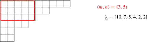
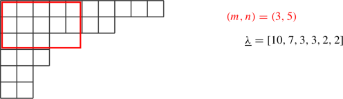
In this specific drawing \(m=4\), \(n=7\), then \(\lambda _1=20\) and \(\lambda _9=1\), while \(\lambda '_1=9\) and \(\lambda '_{20}=1\).
It might be instructive to compare with [45], which also treats all maximally supersymmetric cases together. They use internal labels \((a_\texttt{there},b_\texttt{there})\) where \(a_{there}=\tfrac{1}{2} \gamma {-}\lambda '_2, \quad b_{there}=\tfrac{1}{2} \gamma {-}\lambda '_1\).
The combination \(\lambda +\frac{\theta \gamma }{2}\) appears in the Dynkin diagram (A.14) for the (1, 0) bosonic theory.
This combination is the value appearing in (A.15) sitting on crossed through Dynkin node.
These can be obtained by solving their defining differential equations. In the dual case this is (2.26). For the Jacobi polynomial we refer to [28]. Alternatively, the 1d combinatorial formula in [41] straightforwardly gives the result. The normalisation of the Jacobi is taken such that \(J_{[\lambda ]}=y^\lambda +\ldots \), and this gives the prefactor w.r.t. to the\(~_2F_1\) series.
In fact twisted Harish Chandra functions since we exclude the \((-1)^{\lambda -\beta }\) in the definition of the block.
Notice that \(\textbf{H}_{}\) shows up directly in (5.8), since it is found by replacing \(\textbf{D}_I \rightarrow z_I^2 \partial _I^2 \) and \(\textbf{d}_I\rightarrow \partial _I\). Terms of the Casimir in which \(\textbf{D}_I \rightarrow -z_I^3 \partial _I^2\) and \(\textbf{d}_I\rightarrow -z_I\partial _I\), are generated by the commutator.
Indeed these are the first two Hamiltonians of a tower found in [34], which establishes the classical integrability of the system.
One might worry whether the uplift is unique. For this we can make use of inputs from the physics. In particular, that the Casimir is second order in derivatives, and at most it has degree one under rescaling of \(z_I\). But also knowledge of the operators whose coefficient is a and b dependent, since these come from the Casimir prefactor in (2.5). This reduced possible combinations and helps checking uniqueness.
To do this we use explicit formulae for \(C^-_{\underline{\kappa }}(w;\theta )\) from [26],
$$\begin{aligned} C^{-}_{{\underline{\smash \mu }}}(\theta ;\theta )&= \frac{ \prod _{k=1}^{\mu '_1} \frac{ (\mu _k+\theta (\mu '_1-k)+\theta -1)! }{ (\theta -1)!} }{ \prod _{1\le k_1<k_2\le \mu '_1} (\mu _{k_1}{-}\mu _{k_2}{+}\theta (k_2{-}k_1) )_\theta } \\ C^{-}_{{\underline{\smash \mu }}}(1;\theta )&=\frac{ \prod _{k=1}^{\mu '_1} (\mu _k+\theta (\mu '_1-k))! }{ \prod _{1\le k_1<k_2\le \mu '_1} (\mu _{k_1}{-}\mu _{k_2}{+}\theta (k_2{-}k_1)-(\theta {-}1) )_\theta }\, . \nonumber \end{aligned}$$after which the majority of contributions to \({ \Pi _{{\underline{\smash \mu }}}(\theta ) }\big /{ \Pi _{{\underline{\smash \mu }}+\Box _{ij}}(\theta ) }\) simplify in the ratio.
A posteriori, \(\textbf{f}\) can also be written in terms of the A-type binomial coefficient, built out of the A-type interpolation polynomials of Okounkov [67], which can be seen as the limit \(u=\infty \) in (C.30). The duality \(\textbf{f}\leftrightarrow \textbf{g}\) can be proven using the identification with the A-type binomial coefficient.
As discussed at the end of Sect. 4.2 we believe this is also a certain \(S_n\) combination of Harish Chandra contributions to the corresponding Heckman–Opdam hypergeometric.
The \(C_{\underline{\smash \mu }}^0(w;\theta )\) was defined in (5.38). Here we are giving the final result for \({C^0_{{\underline{\smash \mu }}/{\underline{\smash \lambda }}}(\theta \alpha ;\theta ) C^0_{{\underline{\smash \mu }}/{\underline{\smash \lambda }}}(\theta \beta ;\theta ) }\).
For example, the RHS can be transposed by using
$$\begin{aligned} (T_{-\theta \gamma })^{{\underline{\smash \mu }}'}_{{\underline{\smash \lambda }}'}(\tfrac{1}{\theta },-\theta p_{12},-\theta p_{43} )=\frac{(-)^{|{\underline{\smash \lambda }}|} \Pi _{{\underline{\smash \lambda }}}(\theta ) }{(-)^{|{\underline{\smash \mu }}| }\Pi _{{\underline{\smash \mu }}}(\theta ) }(T_{\gamma })^{{\underline{\smash \mu }}}_{{\underline{\smash \lambda }}}(\theta ,p_{12},p_{43}) \end{aligned}$$which follows from \(\textbf{C}^{(\theta ,a,b,c)}(\textbf{x}|\textbf{y})=-\theta \, \textbf{C}^{(\frac{1}{\theta }, -a \theta ,-b \theta ,-c \theta )}(\textbf{y}|\textbf{x})\), and properties of the (super) Jack polynomials under transposition.
Upon writing \(\left( {T}_{\tilde{\gamma } }\right) _{N^M\backslash {\underline{\smash \lambda }}}^{N^M\backslash {\underline{\smash \mu }}}( {\theta }, -p_{12} ,-p_{43} )\) note that \(C^0_{{\underline{\smash \mu }}/{\underline{\smash \lambda }}}\left( \theta \alpha , \theta \beta ;\theta \right) \) is recovered by using (7.22).
The sum over \({\underline{\smash \lambda }}\) in (8.15) we kept unbounded (since it automatically truncates to \(M^n\)) will now also automatically truncate since \((S^{(M)})_{{\underline{\smash \mu }}}^{{\underline{\smash \lambda }}}=0\) when \({\underline{\smash \mu }}\subset {\underline{\smash \lambda }}\). The result is therefore a polynomial, i.e. the Jacobi polynomial.
This then gives

An equivalent parametrisations, \(\gamma _{ij}=p_i-p_j-2b_{ij}\), counts the number of bridges going from \({\mathcal {O}}_{p_i}{\mathcal {O}}_{p_j}\) to the opposite pair. \(\gamma _{12}+\gamma _{13}+\gamma _{23}=\sum _i p_i\), is a Mandelstam-type constraint for free theory four-point correlators.
Note the difference with the corresponding group theory interpretation of the Jack decomposition (C.59) which is instead equivalent to decomposing reps of \(U(m+m'|n+n')\rightarrow U(m|n)\otimes U(m'|n')\) in the \(\theta =1\) case.
Minkowski superpsace corresponds to the coset space obtained by putting cross through all odd (white) nodes in the relevant super Dynkin diagram rather than the crossed through nodes of analytic superspace (3.3).
In the context of integrability this has been studied in, e.g. [80].
In this paper, we used the limit \(q\rightarrow 1\) and \(t\rightarrow q^\theta \), in the notation of [32].
The limit to the Jacobi polynomials is designed to degenerate the BC interpolation polynomials to Jack polynomials and the q-deformed binomial coefficient to its classical counterpart [41].
We thank Ole Warnaar for pointing out this to us.
This is a change of basis of the matrix form in (A.3).
Note the following useful relations
$$\begin{aligned} \left\{ \begin{array}{cl} z_I&{}=-\frac{1}{4} \left( \frac{1}{\sqrt{ \hat{z}_I} }-\sqrt{ \hat{z}_I } \right) ^{\!\! 2} \\ z_I-1&{}=-\frac{1}{4} \left( \frac{1}{\sqrt{ \hat{z}_I} }+\sqrt{ \hat{z}_I } \right) ^{\!\! 2} \end{array}\right. \qquad ;\qquad \left\{ \begin{array}{lll} \hat{z}_I \frac{\partial z_I}{\partial \hat{z}_I}= &{}\frac{1}{4} \frac{ (1-\hat{z}_I^2 ) }{ \hat{z}_I}&{} = \sqrt{ z_I(z_I-1)} \\ &{}\frac{1}{4}\frac{ (1+\hat{z}_I^2 ) }{ \hat{z}_I} &{}= -(z_I-\frac{1}{2})\end{array}\right. \end{aligned}$$See [29] for a comprehensive introduction.
The skew diagram \({\underline{\smash \lambda }}/\underline{\kappa }\) is sometimes known as a horizontal strip.
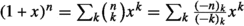
Indeed the Pochhammer symbol \((-z)_k\) is precisely a case of interpolating polynomial, giving the standard one-variable binomial expansion
 .
.Conventionally the supersymmetric filling is also reversed, hence decreasing rather than increasing.
We can also rewrite the above equality as
$$\begin{aligned} \frac{ h^{(\theta )}_{{\underline{\smash \lambda }}+(\theta \tau ')^m}-h_{(\theta \tau ')^m}^{(\theta )}}{2\theta \tau '} +\frac{ h_{{\underline{\smash \lambda }}'+\tau '^n}^{(\frac{1}{\theta })}+ h_{(-\tau ')^n}^{(\frac{1}{\theta })}}{2\tau '}= |m^n|+|\lambda '|+|(\tau ')^n| \end{aligned}$$(C.52)In the limit \(\tau '\rightarrow 0\) the RHS is simply \(\sum _{i=1}^m \lambda _i + \sum _{j=1}^n \lambda '_j\).
This is
$$ C^-_{\underline{\kappa }+(\tau ')^n}(w;\theta )\big / C^-_{\underline{\kappa }}(w;\theta )=C^-_{(\tau ')^n}(w;\theta ) \times C^0_{\underline{\kappa }}(w+\tau '+\theta (n-1);\theta )\big / C^0_{\underline{\kappa }}(w+\theta (n-1);\theta ) $$For the last rewriting consider that \(((\mu _s-m^n)')_i=\mu _{m+i}\) \(\forall i\ge 1\).
These terms are
$$\begin{aligned} \frac{(-)^{|{\underline{\smash \mu }}|+\beta \mu _1} C^-_{{\underline{\smash \mu }}}(\theta ;\theta ) }{ C^0_{{\underline{\smash \mu }}}(\beta \theta ;\theta )C^-_{\mu _1^\beta \backslash {\underline{\smash \mu }}}(\theta ;\theta ) }\times \frac{C^0_{\mu _1^\beta \backslash {\underline{\smash \mu }}}(\beta \theta ;\theta ) }{ C^-_{\mu _1^\beta }(1;\theta ) }\times { C^0_{\mu _1^\beta \backslash {\underline{\smash \mu }}}(-\mu _1;\theta ) C^0_{{\underline{\smash \mu }}}(1+\theta (\beta -1);\theta ) }{}=1 \end{aligned}$$using \(w=\theta \) in (E.8) and \(w=\mu _1\) in (E.7), then again \(w=-\beta \theta \) in (E.7). Finally \((-)^{\beta \mu _1}C^0_{\mu _1^\beta }(-\mu _1;\theta )/C^-_{\mu _1^\beta }(1;\theta )=1\) and \(C^0_{\mu _1^\beta }(\beta \theta ;\theta )/C^-_{\mu _1^\beta }(\theta ;\theta )=1\), directly from their definitions.
Of course the same is true for a symmetric permutation of all variables on the LHS
In [11], see formulae (3.11), (3.18) and (3.19).

 .
.References
Galperin, A., Ivanov, E., Kalitsyn, S., Ogievetsky, V., Sokatchev, E.: Unconstrained N = 2 matter, Yang-Mills and supergravity theories in harmonic superspace. Class. Quant. Grav. 1, 469–498 (1984)[erratum: Class. Quant. Grav. 2, 127 (1985). https://doi.org/10.1088/0264-9381/1/5/004
Howe, P.S., Hartwell, G.G.: A superspace survey. Class. Quant. Grav. 12, 1823–1880 (1995). https://doi.org/10.1088/0264-9381/12/8/005
Hartwell, G.G., Howe, P.S.: (N, p, q) harmonic superspace. Int. J. Mod. Phys. A 10, 3901–3920 (1995). https://doi.org/10.1142/S0217751X95001820. arXiv:hep-th/9412147 [hep-th]
Howe, P.S., Leeming, M.I.: Harmonic superspaces in low dimensions. Class. Quant. Grav. 11, 2843–2852 (1994). https://doi.org/10.1088/0264-9381/11/12/004. arXiv:hep-th/9408062 [hep-th]
Howe, P.S.: Aspects of the D = 6, (2,0) tensor multiplet. Phys. Lett. B 503, 197–204 (2001). https://doi.org/10.1016/S0370-2693(00)01304-6. arXiv:hep-th/0008048 [hep-th]
Heslop, P.J.: Superfield representations of superconformal groups. Class. Quant. Grav. 19, 303–346 (2002). https://doi.org/10.1088/0264-9381/19/2/309. arXiv:hep-th/0108235 [hep-th]
Heslop, P.J., Howe, P.S.: Four point functions in N = 4 SYM. JHEP 01, 043 (2003). https://doi.org/10.1088/1126-6708/2003/01/043. arXiv:hep-th/0211252 [hep-th]
Heslop, P.J.: Aspects of superconformal field theories in six dimensions. JHEP 07, 056 (2004). https://doi.org/10.1088/1126-6708/2004/07/056. arXiv:hep-th/0405245 [hep-th]
Doobary, R., Heslop, P.: Superconformal partial waves in Grassmannian field theories. JHEP 12, 159 (2015). https://doi.org/10.1007/JHEP12(2015)159. arXiv:1508.03611 [hep-th]
Howe, P.S., Lindström, U.: Notes on super killing tensors. JHEP 03, 078 (2016). https://doi.org/10.1007/JHEP03(2016)078. arXiv:1511.04575 [hep-th]
Dolan, F.A., Osborn, H.: Conformal partial waves and the operator product expansion. Nucl. Phys. B 678, 491–507 (2004). https://doi.org/10.1016/j.nuclphysb.2003.11.016. arXiv:hep-th/0309180 [hep-th]
Isachenkov, M., Schomerus, V.: Superintegrability of \(d\)-dimensional conformal blocks. Phys. Rev. Lett. 117(7), 071602 (2016). https://doi.org/10.1103/PhysRevLett.117.071602. arXiv:1602.01858 [hep-th]
Chen, H.Y., Qualls, J.D.: Quantum integrable systems from conformal blocks. Phys. Rev. D 95(10), 106011 (2017). https://doi.org/10.1103/PhysRevD.95.106011. arXiv:1605.05105 [hep-th]
Isachenkov, M., Schomerus, V.: Integrability of conformal blocks Part I. Calogero–Sutherland scattering theory. JHEP 07, 180 (2018). https://doi.org/10.1007/JHEP07(2018)180. arXiv:1711.06609 [hep-th]
Chen, H.Y., Sakamoto, J.I.: Superconformal block from holographic geometry. JHEP 07, 028 (2020). https://doi.org/10.1007/JHEP07(2020)028. arXiv:2003.13343 [hep-th]
Heckman, G.J.: Root systems and hypergeometric functions II. Compos. Math. 64, 329–352 (1987)
Heckman, G.J.: Root systems and hypergeometric functions I. Compos. Math. 64, 353–373 (1987)
Ferrara, S., Grillo, A.F., Parisi, G., Gatto, R.: Covariant expansion of the conformal four-point function. Nucl. Phys. B 49, 77 (1972)
Ferrara, S., Grillo, A.F., Gatto, R.: Tensor representations of conformal algebra and conformally covariant operator product expansions. Ann. Phys. (N.Y.) 76, 161 (1973)
Dobrev, V.K., Mack, G., Petkova, V.B., Petrova, S.G., Todorov, I.T.: On Clebsch Gordan expansions for the Lorentz group in n dimensions. Rep. Math. Phys. 9, 219 (1976)
Mack, G.: D-independent representation of conformal field theories in d dimensions via transformation to auxiliary dual resonance models. Scalar amplitudes. arXiv:0907.2407 [hep-th]
Dolan, F.A., Osborn, H.: Conformal four point functions and the operator product expansion. Nucl. Phys. B 599, 459–496 (2001). https://doi.org/10.1016/S0550-3213(01)00013-X. arXiv:hep-th/0011040 [hep-th]
Dolan, F.A., Osborn, H.: Superconformal symmetry, correlation functions and the operator product expansion. Nucl. Phys. B 629, 3–73 (2002). https://doi.org/10.1016/S0550-3213(02)00096-2. arXiv:hep-th/0112251 [hep-th]
Nirschl, M., Osborn, H.: Superconformal Ward identities and their solution. Nucl. Phys. B 711, 409–479 (2005). https://doi.org/10.1016/j.nuclphysb.2005.01.013. arXiv:hep-th/0407060 [hep-th]
Dolan, F.A., Osborn, H.: Conformal partial wave expansions for N = 4 chiral four point functions. Ann. Phys. 321, 581–626 (2006). https://doi.org/10.1016/j.aop.2005.07.005. arXiv:hep-th/0412335 [hep-th]
Beerends, R.J., Opdam, E.M.: Certain hypergeometric series related to the root system \(BC\). Trans. AMS 339(2), 581–609 (1993)
Macdonald, I.G.: Orthogonal polynomials associated with root systems. Unpublished manuscript 1987; Sém. Lothar. Combin. 45, B45a (2000)
Macdonald, I.G.: Hypergeometric functions I. Unpublished manuscript, 1987; arXiv:1309.4568 [math.CA] (2013)
Macdonald, I.G.: Symmetric Functions and Hall Polynomials, 2nd edn. Oxford University Press, Oxford (1994)
Koornwinder, T.H.: Askey–Wilson polynomials for root systems of type BC. In: Hypergeometric Functions on Domains of Positivity, Jack Polynomials, and Applications. Contemporary Mathematics, vol. 138 , pp. 189–204. American Mathematical Society (1992)
Stokman, J.V., Koornwinder, T.H.: Limit transitions for BC type multivariable orthogonal polynomials. Can. J. Math. 49, 373–404 (1997)
Rains, E.M.: \(BC_n\)-symmetric polynomials. Transform. Groups 10, 63–132 (2005)
Okounkov, A.: \(BC\)-type interpolation Macdonald polynomials and binomial formula for Koornwinder polynomials. Transform. Groups 3, 181–207 (1998)
Sergeev, A.N., Veselov, A.P.: Generalised discriminats, deformed CMS operators and super-Jack polynomials. Adv. Math. 192, 341–375 (2005)
Sergeev, A.N., Veselov, A.P.: Deformed quantum Calogero–Moser problems and Lie superalgebras. Commun. Math. Phys. 245, 249–278 (2004)
Sergeev, A.N., Veselov, A.P.: Deformed Macdonald–Ruijsenaars operators and super Macdonald polynomials. arXiv:0707.3129 [math.QA] (2008)
Moens, E.M., Van der Jeugt, J.: A determinantal formula for supersymmetric Schur polynomials. J. Algebraic Comb. 17(3), 283–307 (2003)
Sergeev, A.N., Veselov, A.P.: BC\(_\infty \) Calogero–Moser operator and super Jacobi polynomials. Adv. Math. 222(5), 1687–1726 (2009). arXiv: 0807.3858 [math-ph]]
R. Doobary, Unpublished notes (2016)
Okounkov, A., Olshanski, G.: Limits of BC orthogonal polynomials as the number of variables goes to infinity. In: Contemporary Mathematics, 417, 281–318, American Mathematical Society, Providence, RI (2006). arXiv:math/0606085 [math.RT]
Koornwinder, T.H.: Okounkov’s BC type interpolation Macdonald polynomials and their q = 1 limit. Sémin. Lothar. Combin. B72a (2015). arXiv:1408.5993 [math.CA]
Mimachi, K.: A duality of Macdonald–Koornwinder polynomials and its application to integral representations. Duke Math. J. 107(2), 265–281 (2001)
Shimeno, N.: A formula for the hypergeometric function of type \(BC_n\). Pac. J. Math. 236(1). arXiv:0706.3555 [math.RT] (2008)
Dolan, F.A., Osborn, H.: On short and semi-short representations for four-dimensional superconformal symmetry. Ann. Phys. 307, 41–89 (2003). https://doi.org/10.1016/S0003-4916(03)00074-5. arXiv:hep-th/0209056 [hep-th]
Dolan, F.A., Gallot, L., Sokatchev, E.: On four-point functions of 1/2-BPS operators in general dimensions. JHEP 09, 056 (2004). https://doi.org/10.1088/1126-6708/2004/09/056. arXiv:hep-th/0405180 [hep-th]
Beem, C., Lemos, M., Liendo, P., Rastelli, L., van Rees, B.C.: The \( \cal{N} =2 \) superconformal bootstrap. JHEP 03, 183 (2016). https://doi.org/10.1007/JHEP03(2016)183. arXiv:1412.7541 [hep-th]
Chester, S.M., Lee, J., Pufu, S.S., Yacoby, R.: The \( \cal{N} =8 \) superconformal bootstrap in three dimensions. JHEP 09, 143 (2014). https://doi.org/10.1007/JHEP09(2014)143. arXiv:1406.4814 [hep-th]
Beem, C., Rastelli, L., van Rees, B.C.: More \({mathcal N }=4\) superconformal bootstrap. Phys. Rev. D 96(4), 046014 (2017). arXiv:1612.02363 [hep-th]]
Lemos, M., Liendo, P., Meneghelli, C., Mitev, V.: Bootstrapping \(\cal{N} =3\) superconformal theories. JHEP 04, 032 (2017). https://doi.org/10.1007/JHEP04(2017)032. arXiv:1612.01536 [hep-th]
Liendo, P., Meneghelli, C., Mitev, V.: Bootstrapping the half-BPS line defect. JHEP 10, 077 (2018). https://doi.org/10.1007/JHEP10(2018)077. arXiv:1806.01862 [hep-th]
Alday, L.F., Chester, S.M., Raj, H.: 6d (2,0) and M-theory at 1-loop. JHEP 01, 133 (2021). https://doi.org/10.1007/JHEP01(2021)133. arXiv:2005.07175 [hep-th]
Lassalle, M.: Explicitation des polynômes de Jack et de Macdonald en longueur trois. C. R. Acad. Sci. Paris Sér. I Math. 333, 505–508 (2001)
Lassalle, M., Schlosser, M.: Inversion of the Pieri formula for Macdonald polynomials. arXiv:math/0402127 (2014). Adv. Math. 202, 289–325 (2006)
Schlosser, M.: Explicit computation of the q,t Littlewood–Richardson coefficients. In: Contemporary Mathematics, vol. 417. American Mathematical Society, Providence (2006).https://www.mat.univie.ac.at/~schlosse/qtlr.html
Howe, P.S., West, P.C.: AdS / SCFT in superspace. Class. Quant. Grav. 18, 3143–3158 (2001). https://doi.org/10.1088/0264-9381/18/16/305. arXiv:hep-th/0105218 [hep-th]
Heslop, P.J., Howe, P.S.: Aspects of N = 4 SYM. JHEP 01, 058 (2004). https://doi.org/10.1088/1126-6708/2004/01/058. arXiv:hep-th/0307210 [hep-th]
Howe, P.S.: On harmonic superspace. Lect. Notes Phys. 524, 68 (1999). https://doi.org/10.1007/BFb0104588. arXiv:hep-th/9812133 [hep-th]
Okazaki, T.: Superconformal Quantum Mechanics from M2-branes. arXiv:1503.03906 [hep-th]
Aprile, F., Santagata, M.: Two-particle spectrum of tensor multiplets coupled to \(AdS_3\times S^3\) gravity. arXiv:2104.00036 [hep-th]
Baston, R.J., Eastwood, M.G.: The Penrose Transform: Its Interaction with Representation Theory
Cornwell, J.F.: Group Theory in Physics, vol. 3. Academic Press, Canbridge (1984)
Rösler, M.: Positive convolution structure for a class of Heckman–Opdam hypergeometric functions of type BC. J. Funct. Anal. 258(8), 2779–2800 (2010). arXiv:0907.2447
https://functions.wolfram.com/HypergeometricFunctions/Hypergeometric2F1/17/02/05/0003/
https://functions.wolfram.com/HypergeometricFunctions/Hypergeometric2F1/17/02/07/0005/
Stanley, R.P.: Some combinatorial properties of Jack symmetric functions. Adv. Math. 77, 76–115 (1989)
Lassalle, M.: Une formule du binôme généralisée pour les polynômes de Jack. C. R. Acad. Sci. Paris Sér. I Math. 310, 253–256 (1990)
Okounkov, A., Olshanski, G.: Shifted Jack polynomials, binomial formula, and applications. Math. Res. Lett. 4, 69–78 (1997)
Yan, Z.: A class of generalized hypergeometric functions in several variables. Can. J. Math. 44, 1317–1338 (1992)
Lassalle, M.: Jack polynomials and some identities for partitions. Trans. Am. Math. Soc. 356, 3455–3476 (2004). arXiv:math/0306222v2 [math.CO]
Caron-Huot, S.: Analyticity in spin in conformal theories. JHEP 09, 078 (2017). https://doi.org/10.1007/JHEP09(2017)078. arXiv:1703.00278 [hep-th]
Matsumoto, S.: Averages of ratios of characteristic polynomials in circular beta-ensembles and super-Jack polynomials. arXiv:0805.3573
Aprile, F., Drummond, J.M., Heslop, P., Santagata, M.: Free theory OPE data from a Cauchy identity (in preparation)
Abl, T., Heslop, P., Lipstein, A.E.: Higher-Dimensional Symmetry of AdS\(_2\times \)S\(^2\) Correlators. arXiv:2112.09597 [hep-th]
Aprile, F., Drummond, J.M., Heslop, P., Paul, H.: Quantum gravity from conformal field theory. JHEP 01, 035 (2018). https://doi.org/10.1007/JHEP01(2018)035. arXiv:1706.02822 [hep-th]
Aprile, F., Drummond, J.M., Heslop, P., Paul, H.: Loop corrections for Kaluza–Klein AdS amplitudes. JHEP 05, 056 (2018). https://doi.org/10.1007/JHEP05(2018)056. arXiv:1711.03903 [hep-th]
Aprile, F., Drummond, J., Heslop, P., Paul, H.: One-loop amplitudes in AdS\(_{5}\times \)S\(^{5}\) supergravity from \( \cal{N} \) = 4 SYM at strong coupling. JHEP 03, 190 (2020). https://doi.org/10.1007/JHEP03(2020)190. arXiv:1912.01047 [hep-th]
Heslop, P., Lipstein, A.E.: M-theory beyond the supergravity approximation. JHEP 02, 004 (2018). https://doi.org/10.1007/JHEP02(2018)004. arXiv:1712.08570 [hep-th]
Abl, T., Heslop, P., Lipstein, A.E.: Recursion relations for anomalous dimensions in the 6d \((2, 0)\) theory. JHEP 04, 038 (2019). https://doi.org/10.1007/JHEP04(2019)038. arXiv:1902.00463 [hep-th]
Beem, C., Lemos, M., Rastelli, L., van Rees, B.C.: The (2, 0) superconformal bootstrap. Phys. Rev. D 93(2), 025016 (2016). https://doi.org/10.1103/PhysRevD.93.025016. arXiv:1507.05637 [hep-th]
Babichenko, A., Stefanski, B., Jr., Zarembo, K.: Integrability and the AdS(3)/CFT(2) correspondence. JHEP 03, 058 (2010). https://doi.org/10.1007/JHEP03(2010)058. arXiv:0912.1723 [hep-th]
Penedones, J., Silva, J.A., Zhiboedov, A.: Nonperturbative Mellin amplitudes: existence, properties, applications. JHEP 08, 031 (2020). https://doi.org/10.1007/JHEP08(2020)031. arXiv:1912.11100 [hep-th]
Sleight, C., Taronna, M.: The unique Polyakov blocks. JHEP 11, 075 (2020). https://doi.org/10.1007/JHEP11(2020)075. arXiv:1912.07998 [hep-th]
Carmi, D., Caron-Huot, S.: A conformal dispersion relation: correlations from absorption. JHEP 09, 009 (2020). https://doi.org/10.1007/JHEP09(2020)009. arXiv:1910.12123 [hep-th]
Caron-Huot, S., Mazac, D., Rastelli, L., Simmons-Duffin, D.: Dispersive CFT sum rules. JHEP 05, 243 (2021). https://doi.org/10.1007/JHEP05(2021)243. arXiv:2008.04931 [hep-th]
Gopakumar, R., Sinha, A., Zahed, A.: Crossing symmetric dispersion relations for Mellin amplitudes. Phys. Rev. Lett. 126(21), 211602 (2021). https://doi.org/10.1103/PhysRevLett.126.211602. arXiv:2101.09017 [hep-th]
Hogervorst, M., Osborn, H., Rychkov, S.: Diagonal limit for conformal blocks in \(d\) dimensions. JHEP 08, 014 (2013). https://doi.org/10.1007/JHEP08(2013)014. arXiv:1305.1321 [hep-th]
Hogervorst, M., Rychkov, S.: Radial coordinates for conformal blocks. Phys. Rev. D 87, 106004 (2013). https://doi.org/10.1103/PhysRevD.87.106004. arXiv:1303.1111 [hep-th]
Schomerus, V., Sobko, E.: From spinning conformal blocks to matrix Calogero–Sutherland models. JHEP 04, 052 (2018). https://doi.org/10.1007/JHEP04(2018)052. arXiv:1711.02022 [hep-th]
Buric, I., Schomerus, V., Sobko, E.: JHEP 01, 159 (2020). https://doi.org/10.1007/JHEP01(2020)159. arXiv:1904.04852 [hep-th]
Burić, I., Isachenkov, M., Schomerus, V.: Conformal group theory of tensor structures. JHEP 10, 004 (2020). https://doi.org/10.1007/JHEP10(2020)004. arXiv:1910.08099 [hep-th]
Burić, I., Schomerus, V., Sobko, E.: JHEP 10, 147 (2020). https://doi.org/10.1007/JHEP10(2020)147. arXiv:2005.13547 [hep-th]
Bergeron, N., Garsia, A.M.: Zonal polynomials and domino tableaux. Discrete Math. 99(1–3), 3–15 (1992)
Olshanetsky, M.A., Perelomov, A.M.: Quantum integrable systems related to lie algebras. Phys. Rep. 94, 313–404 (1983). https://doi.org/10.1016/0370-1573(83)90018-2
Serganova, V.: On generalizations of root systems. Commun. Alg. 24(13), 4281–4299 (1996)
Atai, F., Hallnas, M., Langmann, E.: Orthogonality of super-Jack polynomials and Hilbert space interpretation of deformed CMS operators. arXiv:1802.02016 [math.QA] (2018)
Delduc, F., Magro, M., Vicedo, B.: An integrable deformation of the \(AdS_5 \times S^5\) superstring action. Phys. Rev. Lett. 112(5), 051601 (2014). https://doi.org/10.1103/PhysRevLett.112.051601. arXiv:1309.5850 [hep-th]
Delduc, F., Magro, M., Vicedo, B.: Derivation of the action and symmetries of the \(q\)-deformed \(AdS_{5} \times S^{5}\) superstring. JHEP 10, 132 (2014). https://doi.org/10.1007/JHEP10(2014)132. arXiv:1406.6286 [hep-th]
Arutyunov, G., Frolov, S., Hoare, B., Roiban, R., Tseytlin, A.A.: Scale invariance of the \(\eta \)-deformed \(AdS_5\times S^5\) superstring, T-duality and modified type II equations. Nucl. Phys. B 903, 262–303 (2016). https://doi.org/10.1016/j.nuclphysb.2015.12.012. arXiv:1511.05795 [hep-th]
Koornwinder, T., Sprinkhuizen-Kuyper, I.: Generalized power series expansions for a class of orthogonal polynomials in two variables. Siam J. Math. Anal. 9, 457 (1978)
Ole Warnaar, S.: Bisymmetric functions, Macdonald polynomials and \(sl_3\) basic hypergeometric series. Compos. Math. 144, 271–303 (2008). arXiv:math/0511333v1
Acknowledgements
We would like to thank Ole Warnaar for very illuminating conversations about BC symmetric functions, and guidance into the literature. With great pleasure we would like to thank Reza Doobary for collaboration at an initial stage of this work, and James Drummond, Arthur Lipstein, and Hynek Paul, Michele Santagata for collaboration on related projects over the years. We also thank Chiung Hwang, Gleb Arutunov, Pedro Vieira, Sara Pasquetti, Volker Schomerus and other members of the DESY theory group for discussions on related topics.
Funding
FA is supported by FAPESP grant 2016/01343-7, 2019/24277-8 and 2020/16337-8, and was partially supported by the ERC-STG grant 637844-HBQFTNCER. PH is supported by STFC Consolidated Grant ST/P000371/1 and the European Union’s Horizon 2020 research and innovation programme under the Marie Sklodowska-Curie grant agreement No.764850 “SAGEX”. Both authors contributed equally to the manuscript. No data beyond those presented in this paper are needed to validate its results.
Author information
Authors and Affiliations
Corresponding author
Additional information
Communicated by Horng-Tzer Yau.
Publisher's Note
Springer Nature remains neutral with regard to jurisdictional claims in published maps and institutional affiliations.
Appendices
Super/Conformal/Compact Groups of Interest
Here we give details about the supercoset construction of Sect. 3, and in particular show how the general formalism ties in with the more standard approach in the case of non-supersymmetric conformal blocks.
1.1 \(\theta =1\): SU(m, m|2n)
The SU(m, m|2n) is the simplest family of theories with a supergroup interpretation for any value of m, n positive integers. This corresponds to the case \(\theta =1\).
The supercoset here is the most straightforward of the three general classes: Firstly view the complexified group \(SU(m,m|2n)=SL(2m|2n;{\mathbb C})\) as the set of \((m|2n|m)\times (m|2n|m)\) matrices (this is a straightforward change of basis of the more standard \((2m|2n)\times (2m|2n)\) matrices). Then the supercoset space we consider has the \(2\times 2\) block structure of (3.4) with each block being a \((m|n)\times (m|n)\) matrix (or rearrangement thereof - see footnote 16.) These blocks are unconstrained beyond the overall unit superdeterminant condition: \({\text {sdet}}(G)={\text {sdet}}(H)=1\). So in particular the coordinates \(X^{AA'}\) of (3.6) are unconstrained \((m|n)\times (m|n)\) matrices. Here A and \(A'\) are both superindices carrying the fundamental representation of two independent SL(m|n) subgroups. This supercoset corresponds to the super Grassmannian Gr(m|n, 2m|2n). For more details see [2, 3, 6, 7, 56].
Then a four point function (and in particular the superconformal blocks) can be written in terms of a function of the four points \(X_1,X_2,X_3,X_4\) invariant under the action of G. This in turn boils down to a function of the \((m|n) \times (m|n)\) matrix Z invariant under conjugation (see [7] for more details)
The \(m+n\) eigenvalues \(x_i,y_i\) then yield the \(m+n\) arguments of the superblocks \(B_{\gamma ,{\underline{\smash \lambda }}}\).
Thus any function of Z invariant under conjugation will automatically solve the superconformal Ward identities associated with the four point function. As first pointed out in this context in [7] the simplest way to construct a basis of all such polynomials associated with a Young diagram \({\underline{\smash \lambda }}\) naturally yields (super) Schur polynomials (which are just the Jack polynomials with \(\theta =1\)). The construction is as follows. Take \(|{\underline{\smash \lambda }}|\) copies of \(Z_A^B\) and symmetrise the upper (B) indices according to the Young symmetriser of \({\underline{\smash \lambda }}\). Then contract all upper and lower indices. For example

Inputting the eigenvalues of Z (A.1) into these we obtain (up to an overall normalisation) precisely the corresponding Schur polynomials i.e. Jack polynomials with \(\theta =1\), \(P_{\underline{\smash \lambda }}(\textbf{z};\theta =1)\). This correspondence works for any Young diagram \({\underline{\smash \lambda }}\).
1.2 \(\theta =2: OSp(4m|2n)\)
Details of this supercoset construction can be found (specialised to the \(m=2\) case) in [5, 8]. We summarise here.
When \(\theta =2\) the relevant (complexified) supergroup is OSp(4m|2n) which has bosonic subgroup \(SO(4m) \times Sp(2n)\) with SO(4m) non-compact and Sp(2n) compact. Of physical interest is the case \(m=2\) in which SO(8) is the complexification of the 6d conformal group SO(2, 6) and Sp(2n) is the internal symmetry group for (0, n) superconformal field theories.
The supercoset space is defined by the marked Dynkin diagram (3.12)b (or (3.13)b if \(n=0\)) and can be realised in the block \(2\times 2\) matrix form of (3.4). To see this one needs to realise the group osp(4m|2n) as the set of supermatrices orthogonal wrt the metric J:

Inputting \(M=H\) in the block form of (3.4) into this we find that a is related to d but is itself unconstrained. Thus the Levi subgroup (under which the operators transform explicitly) is isomorphic to GL(2m|n). Similarly, inputting \(M=s(X)\) in the form of (3.6), we find that the coordinates are \((2m|n)\times (2m|n)\) antisymmetric supermatrices
Note that here and elsewhere \(X^T\) denotes the supertranspose \((X^{AB})^T=X^{BA}(-1)^{AB}\). Four-point functions are written in terms of a function of four such Xs, \(X_1,X_2,X_3,X_4\) invariant under OSp(4m|2n). We can use the symmetry to set \(X_3 \rightarrow 0\) and then \(X_2^{-1} \rightarrow 0\). Then we can use the remaining symmetry to set
Finally we end up with the problem of finding a function of \(X_4\) which is invariant under \(X_4 \rightarrow AX_4A^{T}\) where \(AKA^T=K\). The group of matrices satisfying \(AKA^T=K\) is OSp(n|2m). So letting \(Z=X_4K\) we seek functions of Z invariant under conjugation under \(OSp(n|2m)\subset GL(2m|n)\). Ultimately, an invariant function of \(X_1,X_2,X_3,X_4\) will be a function of the eigenvalues of this matrix Z. The eigenvalues of the \(m\times m\) piece of the matrix Z (3.8) are repeated
As always the independent ones yield the m|n arguments of the superblocks (2.7).
This construction again provides a completely manifest way of solving the superconformal Ward identities. Fascinatingly the simplest way to construct a basis of functions solving these Ward identities yields the super Jack polynomials! To construct a basis of such functions in 1-1 correspondence with Young diagrams \({\underline{\smash \lambda }}\) proceed as follows. Take \(|{\underline{\smash \lambda }}|\) copies of \(W=X_4\), and symmetrise all indices according to the Young symmetriser of \(\widehat{\underline{\smash \lambda }}\) the Young diagram obtained from \({\underline{\smash \lambda }}\) by duplicating all rows. Then contract all indices with \(|{\underline{\smash \lambda }}|\) copies of K.
Let us illustrate this with the simplest examples:

Inputting the eigenvalues of Z (A.6) into these we obtain (up to an overall normalisation) precisely the corresponding Jack polynomial with \(\theta =2\), \(P_{\underline{\smash \lambda }}(\textbf{z};\theta =2)\). This correspondence continues for any Young diagram \({\underline{\smash \lambda }}\).
Note that this derivation of superblocks and super Jacks from group theory makes manifest the stability in m, n of both, since they arise from formulae derived from matrices Z of arbitrary dimensions. A combinatoric description of (super)Jack polynomials with \(\theta =2\) along these lines has also been discussed in [92].
1.3 \(\theta =\frac{1}{2}: OSp(4n|2m)\)
The other value of \(\theta \) for which there is a supergroup interpretation for any m, n is \(\theta =\frac{1}{2}\). Here the relevant (complexified) supergroup is OSp(4n|2m), the same complexified group as previously but with the roles of m, n reversed. This has bosonic subgroup \( Sp(2m) \times SO(4n)\) but now with Sp(2m) non-compact (for \(m=2\) this is the complexified 3d conformal group \(Sp(4) \sim SO(5) \sim SO(2,3)\)) and SO(4n) compact the internal subgroup.
The following is then essentially identical to the \(\theta =2\) case but with the role of Grassmann odd and even exchanged. The supercoset space defined by the marked Dynkin diagram (3.12)c (or (3.13)c if \(n=0\)) can also be realised in the block \(2\times 2\) matrix form of (3.4) by realising the group osp(4n|2m) in the following formFootnote 45 :

The Levi subgroup (under which the operators transform explicitly) is isomorphic to GL(m|2n) and the coordinates are \((m|2n)\times (m|2n)\) symmetric supermatrices
Four-point functions are written in terms of a function of four such Xs, \(X_1,X_2,X_3,X_4\) invariant under OSp(4n|2m). We can use the symmetry to set \(X_3 \rightarrow 0\) and then \(X_2^{-1} \rightarrow 0\). Then we can use the remaining symmetry to set
We then are left with a function of \(X_4\) which invariant under \(X_4 \rightarrow AX_4A^{T}\) where \(AKA^T=K\) i.e. under OSp(m|2n). Letting \(Z=X_4K\) we seek functions of Z invariant under conjugation under \(OSp(m|2n)\subset GL(m|2n)\). Thus ultimately, an invariant function of \(X_1,X_2,X_3,X_4\) will be a function of the eigenvalues of this matrix Z. The eigenvalues of the internal \(n\times n\) piece of the matrix Z (3.8) are repeated and the independent eigenvalues yield the m|n arguments of the superblocks (2.7)
As for \(\theta =2\) this construction provides a completely manifest way of solving the superconformal Ward identities naturally giving \(\theta =\frac{1}{2}\) super Jack polynomials! Take \(|{\underline{\smash \lambda }}|\) copies of \(W=X_4\), and symmetrise all indices according to the Young symmetriser of \(\widehat{\underline{\smash \lambda }}\) which is this time the Young diagram obtained from \({\underline{\smash \lambda }}\) by duplicating all columns rather than rows. Then contract all indices with \(|{\underline{\smash \lambda }}|\) copies of K.
In the simplest examples:

Inputting the eigenvalues of Z (A.11) into these we obtain (up to an overall normalisation) precisely the corresponding Jack polynomials with \(\theta =\frac{1}{2}\), \(P_{\underline{\smash \lambda }}(\textbf{z};\theta =\frac{1}{2})\). This correspondence works for any Young diagram \({\underline{\smash \lambda }}\).
As for \(\theta =1,2\) this derivation of superblocks and super Jacks from group theory makes manifest the stability in m, n of both, since they arise from formulae derived from matrices Z of arbitrary dimensions.
1.4 Non-supersymmetric conformal and internal blocks
We conclude our discussion by considering non-supersymmetric conformal and compact blocks. These were first analysed in [11] using an embedding space formalism for Minkowski space. Here we see how an unusual coset representation of Minkowski space relates these cases to the general matrix formalism we have presented.
1.4.1 Conformal blocks \((m,n)=(2,0)\) with any \(\theta \in \mathbb {Z}^+/2\)
Complexified Minkowski space in d dimensions, \(M_d\), can be viewed as a coset of the complexified conformal group \(SO(d+2;\mathbb {C})\) divided by the subgroup consisting of Lorentz transformations, dilatations and special conformal transformations. It is both an orthogonal Grassmannian and a flag manifold and can be conveniently denoted by taking the Dynkin diagram of \(SO(d+2;\mathbb {C})\) and putting a single cross through the first node (see [60])

This crossed-through node represents the group of dilatations and the remaining Dynkin diagram (with the crossed node omitted) represents the Lorentz subgroup \(SO(d;\mathbb {C})\) with \(d=2\theta +2\).
The coset construction for \(\theta =\frac{1}{2},1,2\) in the previous section suggests to start now from the spinorial representation of \(SO(d+2)\), with \(d=2\theta +2\), rather than the fundamental representation. This representation is \(2^{d/2}\) dimensional for d even (the Weyl representation) and \(2^{(d+1)/2}\) dimensional for d odd. In this representation, the coset space can be written in the block form (3.6) and the coordinates X are \(2^{\lceil \theta \rceil } \times 2^{\lceil \theta \rceil }\) matrices. The matrices will be highly constrained in general. The cross-ratios arise as eigenvalues of the matrix Z which are now repeated (due to the constraints, this matches (A.6) for the case \(\theta =2\) when \(m=2,n=0\)):
thus there are always just two independent cross-ratios \(x_{1},x_2\)‘ which become the variables of the conformal blocks in (2.7).
Representations of the conformal group are specified by placing Dynkin weights below the nodes, so for example a fundamental scalar is given by placing a −1 by the first node and zero’s everywhere else. The scalars of dimension \(\Delta \), \({\mathcal {O}}_\Delta \) appearing as external operators in the four-point function (2.5), have a \(-\Delta \) by the first node

The fact that it has a negative Dynkin label is consistent with the fact that this corresponds to an infinite dimensional representation of the (complexified) conformal group (positive Dynkin labels give finite reps). From the diagram one reads off the field representation on Minkowski space: it has dilatation weight \(\Delta \) and is a scalar under the Lorentz subgroup (since it has zero’s under all nodes of the uncrossed part of the Dynkin diagram).
The only reps which occur in the OPE of two such scalars has dimension \(\Delta \) and Lorentz spin l. The corresponding Dynkin diagram is

where the Young tableau \({\underline{\smash \lambda }}\) is at most two row (the only shape consistent with \((m,n)=(2,0)\)) and
Notice again the redundancy in the description in terms of \(\gamma \) and \({\underline{\smash \lambda }}\). The two operators \({\mathcal {O}}_{\gamma ,[\lambda _1,\lambda _2]}={\mathcal {O}}_{\gamma -2k,[\lambda _1+\theta k,\lambda _2+\theta k]}\) give the same representation for any k as long as it leaves a valid Young tableau. We could use this to set \(\gamma =0\) in this case and just have a description in terms of the Young tableau \({\underline{\smash \lambda }}\) only.
Note that there are different ways of realising \(M_d\) as a coset. The above way is a bit complicated for large d. Had we started instead from the fundamental representation of \(SO(d+2)\), the coset construction would be equivalent to the embedding space formalism, in which \(M_d\) is viewed as the space of null \(d+2\) vectors in projective space \(P_{d+1}\). This is the approach used in [11]. This approach does not fit directly into the general \((m,n,\theta )\) matrix formalism we worked out in the previous cases with \(\theta =\frac{1}{2},1,2\) however. In particular the coset is not in the \(2\times 2\) block form of (3.6), and the independent cross-ratios have no natural origin arising from a diagonal matrix.
1.4.2 Internal blocks \((m,n)=(0,2)\) with \(\theta \in 2/\mathbb {Z}^+\)
A very similar case occurs for \(m=0,n=2\), corresponding to internal blocks. Namely instead of four conformal scalars we have four finite dimensional reps of \(SO(4+\frac{2}{\theta })\). Blocks for these were again discussed in Dolan and Osborn [11]. Here the complexified coset space is the same as in the previous case with \(\theta \leftrightarrow \frac{1}{\theta }\) (although the real forms will be different, previously \(SO(2,2+2\theta )\), now \(SO(4+\frac{2}{\theta })\)).

The discussion of these spaces as explicit matrices is also identical to the previous section.
The external states are a specific representation of \(SO(4+2/\theta )\) specified by placing p above the first node and zeros everywhere else. Note that this time the Dynkin label is positive as it is a finite dimensional representation.

The only reps which occur in the ‘OPE’ (in this case equivalent to the tensor product) of two such reps have Dynkin labels

The Young tableau \({\underline{\smash \lambda }}\) is at most two column (the only shape consistent with \((m,n)=(0,2)\) this is a rotation of a standard SL(2) Young tableau) and we have
Again there is redundancy in the description in terms of \(\gamma \) and \({\underline{\smash \lambda }}\) with \({\mathcal {O}}_{\gamma ,[\lambda '_1,\lambda '_2]'}={\mathcal {O}}_{\gamma +2\delta ,[\lambda '_1+\delta ,\lambda '_2+\delta ]'}\) for any \(\delta \) as long as it leaves a valid Young tableau. Here we could use this to force \(\lambda _2'=0\), so only allow 1 column Young tableaux.
From CMS Hamiltonians to the Superblock Casimir
Jack polynomials (in suitable variables) are eigenfunctions of the Hamiltonian of the Calogero–Moser–Sutherland system for \(A_n\) root sytem whilst Jacobi polynomials (as well as dual Jacobi functions/ blocks) are eigenfunctions of the \(BC_n\) root system. Similarly deformed (i.e. supersymmetric) Calogero–Moser–Sutherland (CMS) Hamiltonians of the generalised root systems \(A_{n|m}\) and \(BC_{n|m}\) yield super Jack polynomials and dual super Jacob fucntions (superblocks) as eigenfunctions.
In this section we review the deformed Calogero–Moser–Sutherland (CMS) Hamiltonian associated to generalised root systems and show explicitly how the BC type relates to the super Casimir for superblocks in our theories.
1.1 Deformed CMS Hamiltonians.
The (non-deformed) Calogero–Moser–Sutherland (CMS) operator for any (not necessarily reduced) root system was first given in [93] via the Hamiltonian
where
-
the \(u^I\) are coordinates in a vector space, \(\partial _I:=\partial /\partial u^I\), and the indices are raised and lowered using the Euclidean metric \(g_{IJ}\).
-
the roots \(\{\alpha _I\}\) are a set of covectors (the roots of the root system) and \(R_+\) is the set of positive roots. \(\alpha ^2\) denotes the length squared of root \(\alpha \), \(\alpha ^2= \alpha _I \alpha _Jg^{IJ}\).
-
Finally to each root \(\alpha \) is associated a parameter \(k_{\alpha }\), which is constant under Weyl transformations, so \(k_{w\alpha }=k_{\alpha }\) for w in the Weyl group. For any covector \(\alpha \) which is not a root then we have \(k_{\alpha }=0\).
In [35] this story was generalised and deformed CMS operators were defined in terms of generalized (or supersymmetric) root systems. The irreducible generalized root systems were first classified by Serganova [94]. The generalized root systems are no longer required to have a Euclidean metric but can have non-trivial signature, and they have the analogous relation to Lie superalgebras as root systems do to Lie algberas. In the classification there are just two infinite series, \(A_{m,n}\) and \(BC_{m,n}\) (which we will concentrate on) together with a handful of exceptional cases.
The deformed Hamiltonian has the same form as (B.1) but with some additional subtleties
-
The metric \(g_{IJ}\) need not be Euclidean.
-
There are odd (also known as imaginary) roots which must have \(k_\alpha =1\).
-
There will be relations between some of the parameters \(k_\alpha \) even when they are not related by Weyl reflections.
We will give the two main cases, \(A_{n|m}\) and \(BC_{n|m}\) explicitly in the next subsections.
In all cases there is a special eigenfunction (the ground state) of \(\mathcal {H}\) which takes the universal form,
This is automatic in the non-deformed case but in the deformed case it requires the additional relations between parameters \(k_\alpha \).
It is useful to then write other eigenfunctions of \(\mathcal {H}\) as the product \(\Psi _0 f\) for some function \(f(u_I,\{ k_{\alpha }\})\). The function f is then an eigenfunction of the conjugate operator \(\Psi _0^{-1} {\mathcal {H}} \Psi _0\). This is the one we shall relate to the super Casimir. This conjugate operator also has a universal (and indeed simpler ) form for all such (generalised) root systems
for some constant c.
Our presentation in this appendix collects a number of known results and follows [35]. In addition, we will rewrite the differential operators \(\mathcal {L}\), by using the (orthogonal) measures associated to the root systems.
1.2 A-type Hamiltonians and Jack polynomials
The \(A_{n-1|m-1}\) generalised root system can be placed inside an \(n+m\) dimensional vector space. The positive roots will be parametrised as
where \(e_{I=1,\ldots m+n}\) give the basis of unit vectors. The (inverse) metric is
\(R^{+}_{}\) splits into three separate Weyl orbits (therefore there will be three distinct \(k_{\alpha }\)) and the three families of roots are
Plugging in these, the CMS operator (B.1) thus becomes
where the parity assignment is \(\pi _{i=1,\ldots n}=0\) and \(\pi _{i'=n+1,\ldots n+m}=1\).
The ground state is given by
and the conjugated operator (B.3) is
where \(\rho _{\theta }=\sum _{\alpha } k_{\alpha }\alpha =\sum _{I<J}(-\theta )^{1-\pi _I-\pi _J}(e_I-e_J)\), and \(|\rho _\theta |^2\) is the norm of \(\rho _{\theta }\) under \(g^{IJ}\).
Notice that \(\mathcal {L}^{A}_{}\) contains in principle all terms coming from \(\sum _I (-\theta )^{\pi _I} \partial _I^2 \Psi _0\) and in particular the terms \(\sum _{\beta } \sum _{\alpha \ne \beta } k_{\alpha } k_{\beta }\, (\alpha _I g^{IJ} \beta _J)\, \cot (\alpha ^{}_I u^I) \cot (\beta _I u^I)\), which have mixed nature and do not cancel immediately with the ones from \(\mathcal {H}^A\). However these can be replaced in favour of a \(\theta \) dependent constant, \(-\sum _{\beta } \sum _{\alpha \ne \beta } k_{\alpha } k_{\beta }\, (\alpha _I g^{IJ} \beta _J)\), because of the following relation
This condition is automatically satisfied by the \(k_{\alpha }\) assignment of the roots, and can be understood as a consistency condition on \(\Psi _0\) being the ground state.
Finally, by changing variables to \(z_I=e^{2i u_I}\), we find \(\cot (u_I-u_J)=i(z_I+z_J)/(z_I-z_J)\) and \(\partial _{u_I}=2i z_I \partial _{z_I}\). Therefore,
and one can check that
where \(\textbf{H}_{}\) is defined in (5.9) and is the defining operator of super Jacks (5.12) .
At this point it is also interesting to note that superJack operators are orthogonal in an \(A_{(m,n)}\) measure [95]
(where the parity assignment is \(\pi _{i=1,\ldots n}=0\) and \(\pi _{i'=n+1,\ldots n+m}=1\)) and the A-type CMS operator (B.10) can be rewritten in a very simple way in terms of this measure as
Finally, we point out that Jack polynomials are also eigenfunctions of the one-parameter family of Sekiguchi differential operators [67].
1.3 \(BC_{}\)-type Hamiltonians and superblocks
We now move on to the CMS operator for the generalised BC root system and relate it to the Casimir which give superblocks.
The positive roots of the \(BC_{n|m}\) root system live in an \(m+n\) dimensional vector space and are as follows
where again \(e_{I=1,\ldots m+n}\) are the basis of unit vectors and the inverse metric is the same as in the \(A_{n|m}\) case (B.5). The parameters are assigned as follows,
and
Plugging these values into the general formula (B.1) we obtain the Hamiltonian
where the first line is a trivial modification of (B.7).
The ground state (B.2) becomes
and the conjugated operator is
where \(\rho _{\theta }=\sum _{\alpha } k_{\alpha }\alpha \) and \(\mathcal {D}_{I}=( \partial _{I}+ 2\cot (2u_I) )-2(-\theta )^{-\pi _I} ( p \cot u_I + (2q+1) \cot (2u_I) )\).
Going through the computation notice that for the ground state to be so, the following relation had to be satisfyied
This was not automatic for the \(k_{\alpha }\) assignment but puts a constraint which we used to solve for r and s. The summation over \(\beta \not \sim \alpha \) excludes roots which are parallel in the vector space. The origin of this constraint again can be understood as a rewriting of the potential terms arising from \( \sum (-\theta )^{\pi _I} \partial _I^2 \Psi _0\) coming from mixed products which do not cancel immediately against the potential terms in \(\mathcal {H}^{BC}_{}\).
We now change variables to exponential coordinates \(\hat{z}_I = e^{2iu_I}\), and we get
We can rearrange the sum over many-body interactions as a sum over \(I\ne J\), then for a single derivative we can add up the two terms \(\frac{\hat{z}_I+\hat{z}^{\pm }_J}{\hat{z}_I-\hat{z}^{\pm }_J}\) to find \(\frac{2\hat{z}_J(1-\hat{z}_I^2)}{(\hat{z}_I -\hat{z}_J)(1-\hat{z}_i \hat{z}_J)}\).
Finally we need to change variables again toFootnote 46
and we obtain
At this point we can understand the relation between the super Casimir \(\textbf{C}\), defining the superblocks, and \(\mathcal {L}^{BC}_{}\). One can check that they are closely related after conjugation and a shift

with \(\beta = \min \left( \tfrac{1}{2} (\gamma {-} p_{12}), \tfrac{1}{2} (\gamma {-} p_{43}) \right) \). We have thus shown that the differential operator corresponding to \(BC_{}\) root system is equivalent to our Casimir operator.
Before concluding this section however, we point that there is an analogue of the measure based relation (B.13) in the super BC case which we have not seen in the literature previously. Macdonald used a measure to define \(BC_n\) Jacobi polynomials as orthogonal (see for example [28] page 52). This measure has a natural generalisation to the \(BC_{n|m}\) case as follows
We then find that the operator \(\tfrac{1}{4}\mathcal {L}^{BC}\) has the simple form
where \(p=\theta (p^- - p^+)\) and \(q=-\frac{1}{2}+\theta p^+\). Recall that \(p^{\pm }=\frac{|p_{43}\pm p_{12}|}{2}\) in terms of the external charges.
Symmetric and Supersymmetric Polynomials
In this section we review relevant background regarding Young diagrams and symmetric polynomials (Jacks and interpolation Jacks), both in the bosonic and supersymmetric case. We shall view multivariate Jack polynomials and interpolation polynomials as fundamental, in the sense that they are homogeneous polynomials in certain variables. In particular they can be constructed as a sum over semistandard Young tableaux, or filling, as we will see. On the other hand, Jacobi polynomials (and blocks) we view as ‘composite’: they naturally can be thought of as a sum of Jacks as we have done throughout the paper. In this appendix we focus on the fundamental objects themselves.
1.1 Symmetric polynomials
A Young diagram is a collection of boxes drawn consecutively on rows and columns, with the number of boxes on each row decreasing as we go down, for example

By counting the number of boxes on the rows we define a representation of the Young diagram of the form \({\underline{\smash \lambda }}=[\lambda _1,\ldots ]\). Equivalently, by counting the number of boxes on the columns we define the transposed representation \({\underline{\smash \lambda }}'=[\lambda _1',\ldots ]\). Both \({\underline{\smash \lambda }}\) and \({\underline{\smash \lambda }}'\) are partitions of the total number of boxes. A box \(\Box \) in the diagram has coordinates (i, j) where for each row index i, \(1\le j\le \lambda _i\), and for each column index j, \(1\le j\le \lambda '_i\).
Physics-wise, Jack and Jacobi polynomials are best known as eigenfunctions of known differential operators, but more abstractly, the theory of symmetric polynomials associates polynomials to Young diagrams in such a way that polynomials are characterised by properties and uniqueness theorems [27, 28, 32, 33], which are equivalent to solving the corresponding differential equations.Footnote 47
In this appendix we will highlight a combinatorial definition for Jack and interpolation polynomials, which is very efficient in actual computations. We focus on bosonic polynomials first, for which there is no distinction among \(\{x_1,\ldots x_m\}\) variables, differently from the supersymmetric case discussed afterwards.
For a polynomial P of m variables, the combinatorial formula takes the form
The functions \(\Psi \) and f depend on the polynomials under consideration (i.e. Jack or Interpolation polynomials). Note that in some cases the function \({f}_{}\) may depend explicitly on the integers (i, j) and the integer \(\mathcal{T}(i,j)\), in addition to the variable \(x_{\mathcal{T}(i,j)}\), but we will usually suppress this dependence in order to avoid cluttering the notation. Both \(\Psi \) and f may also depend on various external parameters, which we denoted collectively by \(\textbf{s}\). As a concrete example to have in mind: Jack polynomials have simply \({f}_{}(x,i,j;\theta )= x\) and for the special case with \(\theta =1\) (corresponding to Schur polynomials) the coefficient \(\Psi _\mathcal{T}(\theta =1)=1\).
The sum in (C.2) is over all fillings (also known as semistandard Young tableaux) of the Young diagram \({\underline{\smash \lambda }}\), denoted here and after by \(\{\mathcal{T}\}\). A filling \(\mathcal {T}\) assigns to a box with coordinates \((i,j)\in {\underline{\smash \lambda }}\), a number in \(\{1, \ldots m\}\) in such a way that \(\mathcal{T}(i,j)\) is weakly decreasing in j, which means from left-to-right, and strongly decreasing in i, from top-to-bottom, which means \(\mathcal{T}(i,j)>\mathcal{T}(i-1,j)\), \(\mathcal{T}(i,j)\ge \mathcal{T}(i,j-1)\).
Note that the fillings precisely correspond to the independent states of the U(m) representation \({\underline{\smash \lambda }}\) which one typically views as a tensor with \(|{\underline{\smash \lambda }}|\) indices symmetrised via a Young symmetrizer.
For example, if \({\underline{\smash \lambda }}=[3,1]\) and \(m=2\), the fillings \(\{\mathcal {T}\}\) are

which correspond to the three states in the corresponding rep of U(2), the independent states in a tensor of the form \(S_{abcd} = T_{(abc)d}-T_{(dbc)a}\) where the indices \(a,b,c,d= 1,2\). Then for example the Schur polynomial can be directly read off from (C.2) with \(f(x) =x\) and \(\Psi =1\) as
We immediately see from this definition that if the number of rows of \({\underline{\smash \lambda }}\) is greater than the number of variables m then \(P_{\underline{\smash \lambda }}=0\) since it is not possible to construct a valid semistandard tableaux and the sum is empty (just as for U(m) reps).
In order to define \(\Psi \) it is first useful to note that there is a simple way to generate all the fillings \(\{\mathcal{T}\}\) given a Young diagram \({\underline{\smash \lambda }}\), via recursion in the number of variables m. (See for example the discussion in [67].) This recursion in fact gives a way of generating the polynomial itself also, equivalent to the combinatorial formula (C.2). It reads
where \({\underline{\smash \lambda }}/ \underline{\kappa }\) is the skew Young diagram obtained by taking the Young diagram of \({\underline{\smash \lambda }}\) and deleting the boxes of the sub Young diagram \(\underline{\kappa }\) (see Sect. C.2). Here \(\psi ^{}\) is closely related to \(\Psi \) mentioned above (we will give the precise relation shortly), and the symbol \(\underline{\kappa } \prec {\underline{\smash \lambda }}\) means that \(\underline{\kappa }\) belongs to the following set,Footnote 48
In this formula, if \({\underline{\smash \lambda }}\) is a partition with less than \(m+1\) rows, it is extended with trailing zeros. The recursion generates sequences of Young diagrams of the form
with a strict inclusion, i.e. \(\underline{\kappa }^{(i-1)}\subset \underline{\kappa }^{(i)}\). This is the same as considering the set of fillings \(\{\mathcal{T}\}\). For example, for the above case with \({\underline{\smash \lambda }}=[3,1]\) in (C.3) the sum in (C.5) would be over \(\underline{\kappa }\in \{[3],[2],[1]\}\). These sub Young diagrams are then filled with \(x_1\)’s and the remaining bits \({\underline{\smash \lambda }}/\underline{\kappa }\) filled with \(x_2\) reproducing (C.3).
It follows that for a filling \(\mathcal{T}\) corresponding to a sequence (C.7),
and the recursion and the combinatorial formula (C.2) are the same. In particular l is the level of nesting in the recursive formula. In the example above with \(m+1\) variables, the relation between l and \(\mathcal{T}(i,j)\) is
Given the above facts it is enough for us to define \(\psi ^{}_{{\underline{\smash \lambda }},\underline{\kappa }}\) and the function \(f(x;\textbf{s})\) in order to fully define the symmetric function.
We will now examine the various specific cases, beginning with the Jack polynomials.
1.2 Jack polynomials
Jack polynomials depend on one parameter, \(\theta \). The defining function is (for example [67])
with,
Considering the top-left Pochhammer symbol, notice that \(\psi _{{\underline{\smash \lambda }},\underline{\kappa }}\) vanishes when,
i.e. when one of the terms vanishes. This happens precisely when \(\underline{\kappa }\nprec {\underline{\smash \lambda }}\).
As a simple example then consider \(P_{[2,1]}(x_1,x_2;\theta )\). The case with \(\theta =1\) (Schur polynomial) is given in (C.4). For arbitrary \(\theta \) we need the coefficient \(\Psi _\mathcal{T}(\theta )\) for the three fillings \(\mathcal T\) in (C.3). The first and third filling have \(\Psi =1\) whereas the second has \(\Psi =\tfrac{2\theta }{1+\theta }\) and we thus obtain
Notice that Jack polynomials are stable, i.e. \(P_{{\underline{\smash \lambda }}}(x_1,\ldots x_m,0;\theta )=P_{{\underline{\smash \lambda }}}(x_1,\ldots x_m;\theta )\) as can be shown directly from the combinatorial formula (as well as from their definition as the unique polynomial eigenfunctions of the differential equation (5.12) with eigenvalues and differential operator independent of m, and with the same normalisation).
Also note that Jack polynomials have the following property
It is instructive to prove (C.14) by showing again that both RHS and LHS are eigenfunctions of the \(A_{n}\) CMS operator \(\textbf{H}\) in (5.12). Applying \(\textbf{H}\) on the LHS we simply find the corresponding eigenvalue \(h_{{\underline{\smash \lambda }}+\tau ^m}\). On the RHS we need to consider what happens upon conjugation,
Thus applying \(\textbf{H}\!\cdot \!\) to (C.14) we find
which is an identity, and proves (C.14), since both RHSand l.h.s have the same small variable expansion.
Remark. When there is an ambiguity in the notation, in relation to the supersymmetric case, we will specify \(P^{(m,0)}(\textbf{z};\theta )\) to mean the bosonic Jack polynomial.
1.2.1 Dual Jack polynomials
Jack polynomials are orthogonal but not orthonormal (except when \(\theta =1\) where they reduce to Schur polynomials) under the Hall inner product. The dual Jack polynomials (where dual here denotes the usual vector space dual under the Hall inner product) are thus simply a normalisation of the Jacks, defined so that they have unit inner product with the corresponding Jack. Given a Jack polynomial, the dual Jack polynomial has the form [29]
where, as throughout
1.2.2 Skew Jack polynomials
For one way of defining super Jack polynomials shortly we will also need the concept of skew Jack polynomials.
A skew Young diagram \({\underline{\smash \lambda }}/{\underline{\smash \mu }}\), where \({\underline{\smash \mu }}\subseteq {\underline{\smash \lambda }}\) is obtained by erasing \({\underline{\smash \mu }}\) from \({\underline{\smash \lambda }}\). The Figure below gives a simple example,

Skew Jack polynomials are then defined by a similar combinatorial formula but where one sums only over semi standard skew Young tableaux. Or equivalently by the recursion formula
Notice that \(m+1\ge \lambda '_1-\mu '_1\). The number of variables here is the number of variables that can fill in the Young diagram according to recursion in (C.6). The recursion goes on as long as \({\underline{\smash \mu }}\prec \underline{\kappa }^{(1)} \prec \ldots \prec \underline{\kappa }^{(m)}\prec \underline{\kappa }^{(m+1)}\equiv {\underline{\smash \lambda }}\) and the condition \({\underline{\smash \mu }}\prec \underline{\kappa }^{(1)}\) is non trivial, since it implies that a skew Jack polynomial has the vanishing property
For example, imagine a \({\underline{\smash \lambda }}\) with very long rows, and take a very small \({\underline{\smash \mu }}\), then no horizontal strip of \({\underline{\smash \lambda }}\) will contain \({\underline{\smash \mu }}\). Indeed the minimal diagram \(\underline{\kappa }\) generated by the table (C.6) at each step of the recursion is given by components of \({\underline{\smash \lambda }}\) properly shifted upwards.
An example of a skew Jack polynomial is
Skew polynomials have the property that
1.2.3 Structure constants and decomposition formulae for Jacks
The Jack structure constants \({\mathcal {C}}_{{\underline{\smash \lambda }}{\underline{\smash \mu }}}^{\underline{\smash \nu }}(\theta )\) are defined as follows
For \(\theta =1\) they are just the Littlewood–Richardson coefficients.
Then there are related coefficients \(\mathcal{S}_{{\underline{\smash \nu }}}^{\underline{{\underline{\smash \lambda }}}\,{\underline{\smash \mu }}}(\theta )\) obtained from decomposing skew Jack polynomials into Jack polynomials
The property (C.22) then yields the decomposition formula for decomposing higher dimensional Jacks into sums of products of lower dimensional Jacks
For \(\theta =1\) these decomposition coefficients are also the Littlewood-Richardson coefficients, \({\mathcal {C}}_{{\underline{\smash \lambda }}{\underline{\smash \mu }}}^{\underline{\smash \nu }}(1)=\mathcal{S}_{{\underline{\smash \nu }}}^{\underline{{\underline{\smash \lambda }}}\,{\underline{\smash \mu }}}(1)\), but for general \(\theta \) they are related via normalisation:
Note that the structure constants \({\mathcal {C}}_{{\underline{\smash \lambda }}{\underline{\smash \mu }}}^{\underline{\smash \nu }}(\theta )\) and \(\mathcal{S}_{{\underline{\smash \nu }}}^{\underline{{\underline{\smash \lambda }}}\,{\underline{\smash \mu }}}(\theta )\) do not depend on the dimensions of the Jack polynomials in any of the above formulae.
Also note that if the Young diagram \({\underline{\smash \lambda }}\) is built from two Young diagrams \({\underline{\smash \mu }},{\underline{\smash \nu }}\) on top of each other then the corresponding structure constant is 1:
This can be seen by (C.24) noting that the Jack polynomial of dimension equal to the height of \({\underline{\smash \mu }}\) is equal to the skew Jack
This can be verified from the respective combinatoric formulae.
1.3 Interpolation polynomials
The interpolation polynomials of relevance here (i.e. the BC-type which appear in Sect. 7) depend on two parameters, \(\theta \), and a new one denoted here by u. They can be defined in a very similar way to the Jack polynomials and we will denote them \(P^{ip}_{}(\textbf{x};\theta ,u)\). They are symmetric polynomials in the variables \(\textbf{x}=(x_1,..,x_m)\). Generically \(P^{ip}_{}\) is a complicated, non factorisable polynomial and it is uniquely defined by the following vanishing property
where \(\underline{\delta }=(m{-}1,..,1,0)\). This idea generalises what happens for the Pochhammer symbol \((-z)_\lambda =(-z)(-z+1)\ldots (-z+\lambda -1)\) which vanishes if \(0\le z<\lambda \).Footnote 49
The interpolation polynomial is defined via the combinatorial formula (C.2) (or the equivalent recursion (C.5)) with \(\psi \) exactly the same as for the Jacks (C.10), but with a more complicated x dependence arising from a modified f
where \(\psi _{{\underline{\smash \lambda }},\underline{\kappa }}(\theta )\) is the defining function for Jack polynomials (C.10). Instead, note that f here depends explicitly on (i, j) and l. As in (C.7) the index l labels the nesting and is related to \(\mathcal{T}(i,j)\) via (C.9).
One can see an example of the vanishing property from the above definition: take the last variable \(x_{m}\) and the last row \(i=m\) in (C.31), this contributes with terms which vanish for all \(x_{m}=j-1+u\), where \(j=1,\ldots \kappa _{m}\).
Because of the various shifts in the vanishing property (C.29), it is useful to define the non-symmetric version of the interpolation polynomial \(P^{*}(\textbf{x};\theta ,u)\) by
So the vanishing property (C.29) takes the form
(Recalling however that \(P^*_{{\underline{\smash \mu }}}\) here is no longer symmetric in its variables \(\textbf{z}\).)
This interpolation polynomial is \(\mathbb {Z}_2\) invariant under \(x_i\leftrightarrow -x_i\). It was introduced by Okounkov [33], and re-obtained by Rains [32], using a different approach.
1.4 Supersymmetric polynomials
The general combinatorial formulation of symmetric polynomials outlined in Sect. C.1 has a natural supersymmetric generalisation [34]. This allows in particular to define super Jack polynomials and super interpolation Jack polynomials. The only real modification in the general story is that the definition of a filling (semistandard tableaux) is modified to become a supersymmetric filling (or bitableau) since it has to take into account two alphabets, \(x_1,\ldots x_m\) and \(y_1,\ldots y_n\). Written in terms of the letters \(\textbf{z}\), the labelling is \(z_i=x_i\) for \(i=1,\ldots m\), and \(z_{m+j}=y_j\) for \(j=1,\ldots n\) and the combinatorial formula then looks the same as in (C.2)
but with the sum now over all supersymmetric fillings.
The supersymmetric filling assigns to a box of coordinate (i, j) a number \(\{1,\ldots n+m\}\) such that \(\mathcal{T}(i,j)\) is weakly decreasingFootnote 50 in j, i.e. from left-to-right, and is weakly decreasing in i, i.e. from top-to-bottom. But, if \(\mathcal{T}(i,j)\in \{1,\ldots m\}\), then \(\mathcal{T}(i,j)\) is strictly decreasing in i, i.e. from top-to-bottom, and if \(\mathcal{T}(i,j)\in \{n+1,\ldots n+m\}\), then \(\mathcal{T}(i,j)\) is strictly decreasing in j, i.e. from left-to-right.
Note that the above notion of a supersymmetric filling has a direct relation with states of the supergroup U(m|n) just as the ordinary fillings relate to states of U(m). This can again be clearly seen by representing the U(m|n) irrep \({\underline{\smash \lambda }}\) as a tensor \(T_{A_1 A_2 .. A_{|{\underline{\smash \lambda }}|}}\) with superindices \(A\in \{1,..,m|m+1,..,m+n\}\) and symmetrising the indices in the standard fashion via a Young symmetriser. The only caveat is that when the index \(A \in \{m+1,..,m+n\}\) the index is viewed as ‘fermionic’ and so symmetrising two of them becomes anti-symmetrising and vice versa. The resulting independent states obtained in this way will have a precise correspondence with the supersymmetric fillings.
1.4.1 A first example, \({\underline{\smash \lambda }}=[3,1]\) with \((z_1,z_2|z_3)\).
This has two rows, so we can fill it in as in (C.3), namely

Then we introduce the variable \(z_3=y_1\), once

and twice

These correspond to the states of the U(2|1) rep [3, 1] as can be seen via Young symmetrising as described above.
1.4.2 A second example, \({\underline{\smash \lambda }}=[3,1]\) with \((z_1,z_2|z_3,z_4)\).
Again we can fill \({\underline{\smash \lambda }}\) as in the previous example, with both 3 and \(3\rightarrow 4\). Then we have new fillings in which both \(z_3\) and \(z_4\) appear. These are

and


for a total of \(3+2\times 9+4+7\) fillings. These correspond to the states of the U(2|2) rep [3, 1] as can be seen via Young symmetrising.
The variables \(\textbf{z}=(x_1,\ldots x_m|y_{m+1},\ldots y_{m+n})\) are defined to have a parity \(\pi _{i}=0\) if \(x_i\) and \(\pi _i=1\) if \(y_i\).
A Young diagram \({\underline{\smash \lambda }}\) endowed with an (m, n) structure is a Young diagram \({\underline{\smash \lambda }}\) that has to satisfy the condition \(\lambda _{m+1}\le n\). One can easily check that only then will the diagram allow any supersymmetric filling, and correspondingly only then can it yield a non vanishing U(m|n) rep. This condition implies that the Young diagram has at most a hook shape, with only m arbitrarily long rows and only n arbitrarily long columns. The reps split into two cases,
-
typical Young diagram, i.e. \(\lambda _{m+1}\le n\) such that it contains the rectangle \(n^m\). These correspond to long representations of U(m|n).
 (C.40)
 -
atypical Young diagram, i.e. \(\lambda _{m+1}\le n\) such that it does not contain \(n^m\). These correspond to short representations of U(m|n).
 (C.41)


Typical representations are such that the box with coordinates (m, n) lies in the diagram. The simplest example of an atypical representation is the empty diagram.
In both cases it can be useful to define two sub Young diagrams, by essentially cutting open the diagram vertically after the nth column. We then define the Young diagram obtained from the first n columns and transposing as \({\underline{\smash \lambda }}_s\) and the remaining diagram as \({\underline{\smash \lambda }}_e\). So in the above atypical example:

These sub Young tableaux have a direct interpretation in terms of the corresponding U(m|n) rep. They are simply the corresponding representations of the U(n) and U(m) subgroups of the highest weight state. Or put another way, the highest term in the supersymmetric filling will have only y entries in \({\underline{\smash \lambda }}_s\) and only x entries in \({\underline{\smash \lambda }}_e\).
1.5 Super Jack polynomials
Having outlined the general structure of supersymmetric polynomials let us now specify to the main interest, the super Jack polynomials. We just need to define \(\Psi \) and f in (C.34). To define \(\Psi \) we split the superfilling \(\mathcal T\) of \({\underline{\smash \lambda }}\) into \(\mathcal{T}_1\), the part containing \(m+1,..,m+n\), and the rest \(\mathcal{T}_0=\mathcal{T}/\mathcal{T}_1\). Say that \({\underline{\smash \mu }}\) is the shape of \(\mathcal{T}_1\). Then \(\Psi (\mathcal{T};\theta )\) is defined in terms of the Jack \(\Psi \) as [34]
According to this definition the superJack is given as a sum over all decompositions of the form
where the sum can also be restricted to \({\underline{\smash \mu }}\) such that \(\textrm{max}(\lambda '_j-m,0) \le \mu '_{j}\le \lambda '_j \) with \(j=1,\ldots n\).
Note also that we could construct the superJacks directly from Jack polynomials via their decomposition into U(m) and U(n) reps following [34] (see also [95] for a nice review). Quite nicely [34] showed that this decomposition can be brought to (C.45). From this point of view it might be useful to compare this with the bosonic decomposition (C.22).
Remark. A super Jack polynomial is denoted by \(P_{{\underline{\smash \lambda }}}^{(m,n)}(\textbf{z} ;\theta )\). However, the (m, n) dependence can be read off the variables \(\textbf{z}\), when there are no ambiguities in the notation. When this is the case, we will simply use \(P_{{\underline{\smash \lambda }}}^{}(\textbf{z} ;\theta )\).
Some simple observations which can be seen directly from this formula:
1) If \({\underline{\smash \lambda }}\) fails to have an (m, n) structure, so \((i,j)=(m{+}1,n{+}1)\) is in the Young diagram \({\underline{\smash \lambda }}\), then the superJack vanishes. For any \({\underline{\smash \mu }}\) in the summation, either the box \((m+1,n+1)\) is in \({\underline{\smash \mu }}\), in which case \(Q_{\mu '}=0\) as \({\underline{\smash \mu }}'\) will have \(n+1\) rows, or \((m+1,n+1)\) is in \({{\underline{\smash \lambda }}/ {\underline{\smash \mu }}}\) in which case \(P_{{\underline{\smash \lambda }}/ {\underline{\smash \mu }}}=0\) as \({\underline{\smash \lambda }}/ {\underline{\smash \mu }}\) will have a full column with \(m+1\) elements.
2) When \(m=0\) the sum localises on \({\underline{\smash \mu }}={\underline{\smash \lambda }}\), and since \(P_{{\underline{\smash \lambda }}/{\underline{\smash \lambda }}}=P_{\varnothing }=1\), the superJack polynomial reduces to a (normalised) dual Jack polynomial \((-)^{|{\underline{\smash \lambda }}'|}Q_{{\underline{\smash \lambda }}'}( \textbf{y};\tfrac{1}{\theta })\). When \(n=0\) the sum localises on \({\underline{\smash \mu }}=\varnothing \) and the superJack polynomials reduces to \(P_{{\underline{\smash \lambda }}}(\textbf{x};\theta )\).
1.6 Properties of Super Jack polynomials
1.6.1 Stability
The combinatorial formula makes stability of superJacks manifest. Alternatively, from the fact that the eigenvalue of the A-type CMS differential depends only on the Young diagram, and the uniqueness of the polynomial solution for given Young diagram, we also infer that the super Jack polynomials are stable.
1.6.2 The m and n switch
From the bosonisation of the eigenvalue and a property of the differential operator \(\textbf{H}\), namely
we deduce that \(P_{{\underline{\smash \lambda }}'}(\textbf{y}|\textbf{x}; \frac{1}{\theta })\) has to be proportional to \(P_{{\underline{\smash \lambda }}}(\textbf{x}|\textbf{y};{\theta })\). Looking at the precise normalisations we arrive at
We can also show this more directly from either the combinatorial formula or the decomposition formula (where we further decompose the skew Jacks into Jacks via structure constants, and use some known properties of the structure constants).
1.6.3 Shift transformation of superJacks
We have emphasised that blocks should be invariant under the shift symmetry (2.20). In Appendix D we will show that the coefficients \(T_\gamma \) in the expansion of blocks over Jacks possesses this symmetry, but we thus also require the symmetry for the Jacks themselves in order that the blocks have this symmetry. We consider this here.
Let \({\underline{\smash \lambda }}\) be a typical (m, n) representation, i.e. \(\lambda _m \ge n,\lambda _{m+1}\le n\). Then we consider: 1) the Young diagram obtained by a horizontal shift of \(\theta \tau '\) to the first m rows of \({\underline{\smash \lambda }}\) (on the east), and 2) the Young diagram obtained by a vertical shift of \(\tau '\) to the first n columns of \({\underline{\smash \lambda }}'\) (on the south). We will show that
are proportional to each other, then we will find the proportionality factor.
For the bosonic \(n=0\) Jack polynomials, the above claim follows from (C.16) with \(\tau =\theta \tau '\). We will thus use the same argument, and show that both the LHS and r.h.s in (C.48) are eigenfunctions of \(\textbf{H}\) with both m and n turned on.
So let us see what happens when we apply \(\textbf{H}\) on (C.48). On the LHS we simply find the eigenvalue \(h_{{\underline{\smash \lambda }}+(\tau )^m}^{(\theta )}\). On the RHS we use
Note also that the constant term can be written in terms of the same eigenvalue of \(\textbf{H}\),
(In the bosonic case, \(n=0\), this was \(h^{(\theta )}_{\tau ^m}\)). Then, the action of \(\textbf{H}\) on (C.48) matches because of the identity
Note that this is true only if \(\lambda _m \ge n,\lambda _{m+1}\le n\) ie only for typical, long representations. For example it is clearly false for \({\underline{\smash \lambda }}=[\varnothing ]\), which would read“\(0=2\theta \tau ' |m^n|\)".Footnote 51
Having established that the polynomials in (C.48) are proportional to each other, we only need to fix the proportionality. By considering the first term in the decomposition formula (C.45) the only change to take into account is the \(\Pi \) function inside Q for the lowest representation. Following this through we arrive at the shift formula (D.8)
where we are using \(\Pi _{{\underline{\smash \nu }}}^{-1}(\frac{1}{\theta })=\Pi _{\nu '}(\theta )\), and we introduced
as in (C.42).
1.6.4 Super Jacks and the superconformal Ward identity
The uplift of Jack to superJack polynomials follows from a characterisation theorem, cf. Theorem 2 of [34]. In particular, a superJack polynomial \(P_{{\underline{\smash \lambda }}}(\textbf{x}|\textbf{y};\theta )\) is generated by the map \(\varphi _{(m,n)}\) which acts on the power sum decomposition of \(P_{{\underline{\smash \lambda }}}(\textbf{z};\theta )\) as
Note that this map is very easy to understand in the cases \(\theta =1,2,\frac{1}{2}\) where there is a group theoretic interpretation. For example, when \(\theta =1\) we consider the symmetric polynomials as functions of the \(n\times n\) matrix Z, invariant under conjugation \(f(Z)=f(G^{-1}Z G)\), with \(z_i\) the eigenvalues of Z. Then the supersymmetric case just corresponds to the case where Z is a \((m|n)\times (m|n)\) supermatrix and the map \(\varphi \) is just taking the supertrace (see (A.1) and the following discussion). So for example the power sums
A similar discussion also follows in the cases \(\theta =2\) and \(\theta =\frac{1}{2}\) (which is dual under the m, n swap) with the only real difference as far as power sums is concerned being that there are repeated eigenvalues of Z in these cases, which accounts for the factors of \(\theta \) appearing. (See (A.6) and the following for the \(\theta =2\) case and (A.11) for the \(\theta =\frac{1}{2}\) case.)
The characterisation (C.55) implies that superJack polynomials satisfy the condition
From the point of view of the four point functions invariant under the superconformal group, this condition is a consequence of the super-conformal Ward identity. We understand in this way that our construction of the superconformal blocks, as given by the series over super Jack polynomials, automatically satisfy the super-conformal Ward identity. Our approach here is alternative to various other approaches which instead use the superconformal Ward identity to fix the superblock, given an ansatz of \(m\otimes n\) bosonic blocks. We will consider this approach in Appendix 9.
1.6.5 Structure constants and decomposition formulae for super Jacks
The super Jacks (from stability) have exactly the same structure constants as the Jacks. So (C.23) is true for superJacks
and furthermore so is the decomposition formula for decomposing higher dimensional super Jacks into sums of products of lower dimensional super Jacks
Here the arguments of the superJack on the LHS are split between the two superJacks on the RHS e.g. \( P_{{\underline{\smash \mu }}}^{(m|n)}(x_1,..,x_m|y_1,..,y_n)\) and \( P_{{\underline{\smash \nu }}}^{(m'|n')}(x_{m+1},..,x_{m+m'}|y_{n+1},..,y_{n+n'})\). The coefficients \({\mathcal {S}}_{\underline{\smash \lambda }}^{{\underline{\smash \mu }}{\underline{\smash \nu }}}(\theta )\) are completely independent of \(m,m',n,n'\) and are related to the structure constants just as before (C.26)
Indeed the definition of superJacks itself in terms of Jacks (C.45) is just an example of this decomposition with \(n=m'=0\) (after using (C.47) with \(n=0\)).
Note that in the \(\theta =1\) case this corresponds to the decomposition of \(U(m+m'|n+n') \rightarrow U(m|n)\otimes U(m'|n')\) for which the coefficients are the Littlewood Richardson coefficients.
1.7 Super interpolation polynomials
The last polynomials we review are the super interpolation polynomials which we first discuss below (7.29). These were first introduced in [38], and we will repeat below the definition given in [38] following our conventions.
Introduce the bosonic polynomial,
where the corresponding function f follows from (C.31), i.e.
where \(\mathcal{T}(i,j)=1+m-l\). In the main text, see (7.29), we wrote
The supersymmetrised version of \({\hat{I}}\) has the same structure as (C.45), simply reflecting the underlying sum over superfillings, and it is simply
In particular, we find \( \hat{I}^{(0,n)}_{{\underline{\smash \lambda }}}(|\textbf{y};\theta ,h)= (-\theta ^2)^{|{\underline{\smash \lambda }}|} \Pi _{{\underline{\smash \lambda }}'}(\frac{1}{\theta }) {\tilde{P}}^{*(n)}_{{\underline{\smash \lambda }}'}(\ldots y_n;\frac{1}{\theta } ,\tfrac{1}{2}+\tfrac{1}{2\theta }-\tfrac{h}{\theta } ) \), and for \(n=0\) we obvious recover \(\hat{I}_{{\underline{\smash \lambda }}}^{(m)}\). Note that if we take the scaling limit \(z\rightarrow \epsilon z\) and we look at the leading contribution as \(\epsilon \rightarrow \infty \), that polynomial is a superJack, i.e.
Following Veselov and Sergeev, we now define
This object is such that
where \({\underline{\smash \mu }}_s=[\mu '_1,.., \mu '_{{N}}]\) and \({\underline{\smash \mu }}_e\equiv {\underline{\smash \mu }}/{\underline{\smash \mu }}'_s=[(\mu _1 {-} {N})_+,..,(\mu _{{M}} {-} {N})_+]\) where \((x)_+\equiv \max (x,0)\). Note also that the leading contribution of I now gives a superJack polynomial through the relation in (C.47). In the main text, see (7.30), we wrote
with I being the supersymmetrisation we were looking for. Finally
The r.h.s. of course does not depend on (m, n) and it becomes (7.7) upon matching the parameters.
More Properties of Analytically Continued Superconformal Blocks
1.1 Shift symmetry of the supersymmetric form of the recursion
We would like the supersymmetric recursion (6.8) to be invariant under the supersymmetric shift:
This is almost the case for (6.8). The issue is to do with normalisation and we will fix it below. Let us emphasise first that this shift symmetry arises directly from the group theory in all cases with a group theory interpretation, \(\theta =\frac{1}{2},1,2\) (see (3.18)) but we expect it for any \(\theta \). Note that in writing (D.1), we are implicitly assuming that the Young diagram, prior to analytic continuation, contains the box with coordinates (m, n). Thus in a supersymmetric theory we are looking at typical or long representations.
We claim that the following normalisation of \(T_\gamma \) gives a shift invariant result:
where we split the diagrams into east and south components by taking the corresponding first m rows and first n columns. We might consider \({\underline{\smash \lambda }}_e\rightarrow {\underline{\smash \lambda }}_e-n^m\), however this is not important here.
So the claim is that \(T^\texttt{long}_{\gamma }\) is invariant under the shift (D.1). In particular, it solves the following recursion

Note that \(\textbf{c}^{(j)}_{{\underline{\smash \mu }}}(\theta )\) is built out of arm and leg length symbols, \( c_{{\underline{\smash \nu }}}(i,j)=\nu _i-j+(\nu '_j-i+1)/\theta \) and \(c'_{{\underline{\smash \nu }}}(i,j)=\nu _i-j+1+(\nu '_j-i)/\theta \) for \({\underline{\smash \nu }}={\underline{\smash \mu }},({\underline{\smash \mu }}'+\Box _j)'\). This \(\textbf{c}^{(j)}_{{\underline{\smash \mu }}}(\theta )\) is now invariant under (D.1) since it mixes rows and columns coherently, i.e.
The origin of the normalisation in (D.2) can be understood starting from the Casimir differential equations and the super Jack polynomials. Indeed, a quick way to see the invariance of the superblocks under (D.1) is to consider that the eigenvalue of the original Casimir operator on \(B_{\gamma ,{\underline{\smash \lambda }}}\) (2.11)
with \(e=+\frac{\theta \gamma }{2}\) and \(s=-\frac{\gamma }{2}\), is indeed invariant under (D.1). To see this, the hybrid form of the RHS is useful, therefore \(|\gamma |=\sum _{i=1}^m \lambda _i + \sum _{j=1}^n \lambda '_j -nm\), and for \(h_{{\underline{\smash \lambda }}}(\theta )\) the expression given in (5.26).
The precise statement about shift invariance of the long superconformal blocks is
The \(\Pi \) factors follow from the fact that we normalise our blocks so that the coefficient of the leading superJack \(P_{{\underline{\smash \lambda }}}\) is unity, i.e. \(B_{\gamma ,{\underline{\smash \lambda }}}=(\prod x_i^\theta \big /\prod _j y_j)^{\frac{\gamma }{2}} \big ( P_{{\underline{\smash \lambda }}}+\ldots \big )\), and from the analogous relation proved in Appendix C.6 for super Jack polynomials, namely
From (D.7) and (D.8) we find the corresponding transformation on the coefficients
This gives the normalisation of \(T^\texttt{long}_{\gamma }\) in (D.2), so that it is invariant under the shift
We could then define normalised long super Jack polynomial \(P_{{\underline{\smash \lambda }}}^\texttt{long}\) so that \((T^\texttt{long}_{\gamma })\) gives the expansion coefficients and all formulae are manifestly shift symmetric.
Finally, let us point out that the ratio of \(\Pi \) functions in (D.9) should simplify because it does not depend on \(\gamma \). Indeed, by using a property of \(C^-\) under shiftsFootnote 52 and rearranging the expression we obtain
As expected the ratio of \(\Pi \) functions above is more explicitly just a function of the skew diagrams.
1.2 Truncations of the superconformal block
An (m, n) superconformal block \(B_{\gamma ,{\underline{\smash \lambda }}}\) has been so far defined as the multivariate series
In this section we discuss how the infinite sum over \({\underline{\smash \mu }}\) depends effectively on the external parameters \(\alpha ,\beta \) and \({\underline{\smash \lambda }}\). Let us recall indeed that the \(\alpha \) and \(\beta \) dependence of \(T_{\gamma }\) is solved by the \(C^0\) factors, as we pointed out already in Sect. 5.4. Thus
where \(T^\mathtt{\, rescaled}_\gamma \) is \(\alpha ,\beta \) independent. The observation we will elaborate on is that the \(C^0\) factors have certain vanishing properties which in practise truncate the sum.
Given the various forms of the recursions, spelled out in previous sections, it is useful to put the \(C^0\) factors accordingly. To do so consider the equivalent rewritingsFootnote 53
which follow from the definition in (5.38). Then, let us note that \(C^0\) has the following analytic continuation,
therefore, if we consider the (m, 0) analytic continuation of Sect. 6, we are keeping fixed the number of rows of \({\underline{\smash \lambda }},{\underline{\smash \mu }}\), as for the Young diagrams, and we find that \(C^0_{{\underline{\smash \mu }}/{\underline{\smash \lambda }}}(w;\theta )\) has the correct (m, 0) analytic continuation. If instead we consider the (0, n) analytic continuation, we are keeping fixed the number of columns of \({\underline{\smash \lambda }},{\underline{\smash \mu }}\), and thus it is \(C^0_{{\underline{\smash \mu }}'/{\underline{\smash \lambda }}'}(-\tfrac{w}{\theta };\tfrac{1}{\theta })\) on the RHS of (D.14) the one with the correct (0, n) analytic continuation. Finally, the rewriting on the RHS of (D.15) is the one with the correct (m, n) analytic continuation.
To appreciate the vanishing properties of the \(C^0\) factors in (D.13), consider for example \(C^0_{{\underline{\smash \mu }}/{\underline{\smash \lambda }}}(\theta \alpha ;\theta )\). It will vanish when
and similarly for \(C^0_{{\underline{\smash \mu }}/{\underline{\smash \lambda }}}(\theta \beta ;\theta )\). In particular, it is enough that only one factor becomes zero. This of course depends on the values of \(\alpha \), \(\beta \), \(\theta \), as well as \({\underline{\smash \lambda }}\). The general situation is summarised by the following tables. On the east

with w here being either \(\beta \) or \(\alpha \). This means that when the condition is satisfied on a row index i, by progressively increasing \(\mu _i=\lambda _i+n_i\) by integers \(n_i\) we will hit a vanishing point. Similarly on the south
where again w is either \(\beta \) or \(\alpha \).
Consider now a situation with a group theory interpretation, thus relevant for superconformal blocks. Assume first that \({\underline{\smash \lambda }}\) is a Young diagram, then \({\underline{\smash \lambda }}\) has at most \(\beta \in \mathbb {N}\) rows (since in our conventions \(\beta \le \alpha \)). In particular, \(\lambda '_j-\beta \le 0\). From (D.19) with \(j=1\) we thus find \(\mu '_1\le \beta \), and we conclude that there is a vertical cut off on the Young diagrams \({\underline{\smash \mu }}\) over which we sum. On the contrary, note that by construction \(\lambda _i+\theta \beta \ge \theta (i-1)\), \(\forall \) \(i\le m\le \beta \), i.e. the opposite of the condition in (D.18), precisely because \(\beta \) sets the value for the maximal number of rows. Therefore there is no truncation on the horizontal east directions. The picture to have in mind for the superconformal blocks is thus

A posteriori, the cut-off on the south is expected, because the internal subgroup of the superconformal algebra is compact. Note also that for Young diagrams, since T only depends on diagrams, we can see that a solution \((T_{\gamma })_{{\underline{\smash \lambda }}}^{{\underline{\smash \mu }}}\) where \({\underline{\smash \mu }}\) has more than \(\beta \) rows does not exist, by considering an equivalent reasoning on the east. In fact, when \(i=\beta +1\) and \(\lambda _{i=\beta +1}=0\), we find from (D.18) that \(\mu _i=0\).
Consider now a long block with analytically continued \({\underline{\smash \lambda }}\), according to an (m, n) structure, in such a way to describe an anomalous dimension. In this case we still require finiteness of the sum (D.12) on the south, as expected for a compact group. From (D.19) we see then that even when \(\beta \) and \(\lambda '_j\) are generic, if however \(0\le \beta -\lambda '_{j=1,\ldots n}\in \mathbb {Z}^+\), the condition on the truncation can be satisfied. Note instead that our Young diagram argument on the east (D.18) now will not work, precisely because \(\beta \) is not integer for cases of physical interest where \(\lambda _i>0\). We notice however that taking the \(\lambda _i<0\) it woud be possible to have truncation on the east and the south simultaneously and perhaps this reproduces the Sergeev–Veselov super Jacobi polynomials.
The generic ‘shape’ of a physical superconformal block is thus the one illustrated in (D.20).
Revisiting Known Blocks with the Binomial Coefficient
Our formula for the coefficients \((T_{\gamma })_{{\underline{\smash \lambda }}}^{{\underline{\smash \mu }}}\) in (7.12), written in terms of interpolation polynomials, is valid for any Young diagram. We find instructive to test (7.12) against known analytic solutions of the recursion, such as the rank-one and rank-two bosonic blocks. Then, we will repeat a similar check for the determinantal solution found in [9] for \(\theta =1\).
We will use the rescaled version of it, where we omit the dependence on \(\alpha \) and \(\beta \). Therefore,
where
As pointed out already, the interpolation polynomials encode the non-factorisable \(\gamma \) dependence of \((T_{\gamma })_{{\underline{\smash \lambda }}}^{{\underline{\smash \mu }}}\), which we saw emerging experimentally from the recursion. However, the way the interpolation polynomials are evaluated is quite different compared with the recursion. In fact, in order to match \((T_{\gamma })_{{\underline{\smash \lambda }}}^{{\underline{\smash \mu }}}\) we will need to compute \(P^*\) of \(N^M\backslash {\underline{\smash \mu }}\), rather than looking recursing over \({\underline{\smash \mu }}/{\underline{\smash \lambda }}\), as we do in the recursion. Our exercise here will show in simple cases how these two combinatorics actually produce the same result.
Through this section, we shall take the minimal choice for N and M in the above formulae, i.e.
where \(\beta \) as usual fixes the maximal height of both \({\underline{\smash \lambda }}\) and \({\underline{\smash \mu }}\).
1.1 The half-BPS solution
The simplest case to start with is the derivation from (E.1) of the half-BPS solution in (5.37),
To obtain the \(\gamma \) dependence we need consider the ratio of interpolation polynomials in (E.1) and since \({\underline{\smash \lambda }}=[\varnothing ]\), the numerator \(P^*\) is evaluated on \(\mu _1^\beta \), which is a “constant" Young diagram. This evaluation is known. From [32] we find
which we need here for \(c=\mu _1\) and \(\ell =\beta \). For what concerns the denominator instead, this is always factorised for any \({\underline{\smash \lambda }}\) and it is given by (7.7). Putting together we find,
where we rewrote \(C^+_{}\) in terms of \(C^0\) using the explicit definition (7.9), and the fact that the Young diagram involved is a rectangle \(\mu _1^{\beta }\). At this point, the \(1/C^0(\theta \gamma ;\theta )\) comes out thanks to the identity,
taken with \(w=-\theta \gamma \), and the \((-1)^{|{\underline{\smash \mu }}|}\) cancels against the one in (E.2). Finally, the contribution \(1/C^-_{{\underline{\smash \mu }}}(1;\theta )\) comes from \(\Pi _{{\underline{\smash \mu }}}(\theta )\) in (E.2). The remaining terms in the binomial coefficient necessarily have to simplify to unity. When we collect them all,Footnote 54 upon using another identity
we finally obtain our desired result.
Already in this simple example we needed several identities between \(C^{\pm ,0}\) coefficients. This shows that the rewriting of T in terms of interpolation polynomials is quite non trivial.
1.2 Rank-one and rank-two
After the half-BPS solution, we will consider the rank-one cases, since these are fully factorised. Next, the rank-two case, which involves a\(~_4F_3\) and has non trivial dependence on \(\gamma \). Thus it is the most interesting case for our purpose. Our task will be to revisit the solution found by Dolan and Osborn in [11].
1.2.1 Rank-one (1, 0)
For the single row case \(\beta =1\), with \({\underline{\smash \mu }}=[\mu ]\) and \({\underline{\smash \lambda }}=[\lambda ]\), we find
which simplifies to a sign. Then, for the interpolation polynomials we find
in particular, the numerator is trivial, and the denominator follows straightforwardly from (7.7) and (7.9). Putting together the two results above we obtain the formula
which coincides with the one derived in Sect. 4.1.
This case was quite immediate and the reason is that the formula for the \(P^*\) is oriented on the east, as the (1, 0) theory. We will see now what happens in the (0, 1) theory.
1.2.2 Rank-one (0, 1)
For the single column case, the diagrams are \({\underline{\smash \lambda }}=[1^{\lambda '}]\) and \({\underline{\smash \mu }}=[1^{\mu '}]\). This is a case in which \(\lambda ',\mu '\le \beta \). Let us proceed with a direct computation starting with (E.1). The normalisation (E.2) becomes
For the ratio of interpolation polynomials the diagrams are \(\mu _1^\beta \backslash {\underline{\smash \mu }}=[1^{\beta -\mu '}]\) and \(\mu _1^\beta \backslash {\underline{\smash \lambda }}=[1^{\beta -\lambda '}]\) and the polynomials have \(\beta \) variables. This time the numerator involves a non trivial Young diagram, which however has less than \(\beta \) rows. To simplify the result we use the non-trivial reducibility property for the interpolation polynomials, which reads
where r is counting the excess between the number of variables \(\beta \) and the non zero parts of \(\underline{\kappa }\).Footnote 55 In our case, the above result gives back an evaluation formula to
and in fact the RHS follows from (E.5). Thus, the ratio of interpolation polynomials contributes as,
Putting it all together, the final result for \(T^\texttt{rescaled}_{\gamma }\) (defined in (5.45)) is
This coincides precisely with the one derived in Sect. 4.1 for \((T_{\gamma })_{[1^{\lambda '}]}^{[1^{\mu '}]}\) when we re-insert
properly oriented towards the south.
1.2.3 Rank-two (2, 0)
In the rank-one cases there is no room for any non trivial polynomial in \(\gamma \). The first non trivial case in this sense is then rank-two, corresponding to \(T_\gamma \) for two row Young diagrams. The recursion (5.35) for this case was solved explicitly by Dolan and Osborn [11]. They did this first on a case by case basis in dimensions \(d=2,4,6\), then for general \(\theta \) by using properties of the\(~_4F_3\) function, and manipulations inspired by those in [99].Footnote 56 We will show here how this relates to the interpolation polynomial of (7.12).
In our conventions the solution of [11] reads
with
where \({\underline{\smash \lambda }}=[\lambda _1,\lambda _2]\), \({\underline{\smash \mu }}=[\mu _1,\mu _2]\), and \(\kappa _{\pm }=\kappa _1\pm \kappa _2\), for \(\underline{\kappa }={\underline{\smash \lambda }},{\underline{\smash \mu }}\).
The contribution denoted by D is the translation to our conventions of the result of [11], where we implemented the shift symmetry and slightly rewrote some Pochhammers. Note that the\(~_4F_3\) has a series expansion which truncates at \(\min (\lambda _-, \mu _-)\) and can thus be written as the explicit finite sum

Now compare this expression with our expression for \(T_{\gamma }\) written in terms of interpolation polynomials (7.12) (with \(N=\mu _1\), \(M=2\)):
(Note that the shift symmetry shows up nicely in this formula since we can always put together combinations of the form \(\kappa _i+\frac{\theta }{2}\gamma \), and \(\mathcal {N}\) is automatically invariant.) All contributions in (E.21) coming from the denominator and the normalisation, can be straightforwardly computed, and written as product of Pochhammers or Gamma functions. The \(BC_2\) interpolation polynomial in the numerator is also known explicitly, and described by a \(~_4F_3\) [41],

Although similar, this \(~_4F_3\) is not identical to that of (E.19). Also note that it is not manifestly \(w_1 \leftrightarrow w_2\) invariant even though the polynomial is symmetric under this interchange. We thus have two possibilities leading to the same result. Using \(P^{ip}_{[\mu _1-\mu _2]}( w_2,w_1)\) we find
which becomes the same hypergeometric as in (E.19) upon using the Whipple identity
Similarly had we chosen \(P^*_{[\mu _1-\mu _2]}( w_1,w_2)\) a different \({}_4F_3\) identity will give the same final result. Thus we see how the\(~_4F_3\) of [11] arises directly from the interpolation polynomial.
It is quite spectacular to implement on a computer the above representation of \(T_{\gamma }\) and the one arising directly from the recursion and check that they agree over many examples.
1.3 Revisiting the \(\theta =1\) case and determinantals
The superconformal blocks for the case \(\theta =1\) and any (m, n) were obtained in [9]. One of the main outcomes of that derivation is an explicit expression for the coefficients in an expansion over super Schur polynomials, that we quote here below,
We can also conveniently rewrite the above formula for the coefficients as a determinant
In this section we want to directly show how \(({R}_{\gamma })_{{\underline{\smash \lambda }}}^{{\underline{\smash \mu }}}\) also arises from the interpolation polynomials via (7.12), namely we want to show
Notice that for \(\theta =1\) the normalisation simplifies massively,
and only the ratio of interpolation polynomials is important.
Let us begin by improving the expression of the determinant in such a way as to extract the same normalisation. Using \((a)_x=\Gamma [a+x]/\Gamma [a]\), it is simple to realise that various contributions depend solely on either row or column index, therefore can be factored out, and rearranged. We arrive at the expression
Our formula for \(T_{\gamma }\) in terms of interpolation polynomials can be manipulated quite explicitly when \(\theta =1\), since the BC interpolation polynomials for \(\theta =1\) themselves also have a determinantal representation [40],
The entries of the matrix are single-variable interpolation polynomials \(P^{ip}_{\kappa }(w_i,u)\). These do not depend on \(\theta \) and are given by a pair of Pochhammers,
The denominator of (E.30) is the \(\mathbb {Z}_2\) invariant Vandermonde determinant.
We can now proceed and compute \((T_{\gamma })_{{\underline{\smash \lambda }}}^{{\underline{\smash \mu }}}\) for \(\theta =1\). Since we already identified the normalisation, we will focus on \(({R}^\texttt{rescaled}_{\gamma })_{{\underline{\smash \lambda }}}^{{\underline{\smash \mu }}}\). This has to agree with
The idea is simple: we need to recognise the matrix in (E.29). To do so, we first use the expression of the \(BC_1\) interpolation polynomials given in (E.31), and pass from Pochhammers to \(\Gamma \) functions. The result is
where \(J=\beta +1-j\) and the signs have been factored out since only depended on the column index. For the same reason we can factor out \(\Gamma [i-\lambda _i+\mu _1 ] \Gamma [1-i+\gamma +\lambda _i-\mu _1]\) and cancel it between numerator and denominator. Moreover we can reverse the columns and switch \(j\leftrightarrow J\). We arrive at the simple formula
Comparing this result with (E.29) we are left with the statement
But notice that \(\Gamma [1+i-j-\lambda _i+\lambda _j]^{-1}\), because \(\lambda _{i}\ge \lambda _{i+1}\), makes the matrix on the r.h.s a triangular matrix, and the identity follows. Thus \((T^\texttt{rescaled}_{\gamma })_{{\underline{\smash \lambda }}}^{{\underline{\smash \mu }}} =({R}^\texttt{rescaled})_{{\underline{\smash \lambda }}}^{{\underline{\smash \mu }}}\) and our proof is concluded.
Rights and permissions
Springer Nature or its licensor (e.g. a society or other partner) holds exclusive rights to this article under a publishing agreement with the author(s) or other rightsholder(s); author self-archiving of the accepted manuscript version of this article is solely governed by the terms of such publishing agreement and applicable law.
About this article

Cite this article
Aprile, F., Heslop, P. Superconformal Blocks in Diverse Dimensions and BC Symmetric Functions. Commun. Math. Phys. 402, 995–1101 (2023). https://doi.org/10.1007/s00220-023-04740-7
Received:
Accepted:
Published:
Issue Date:
DOI: https://doi.org/10.1007/s00220-023-04740-7