
Abstract
We consider a class of non-integrable 2D Ising models whose Hamiltonian, in addition to the standard nearest neighbor couplings, includes additional weak multi-spin interactions which are even under spin flip. We study the model in cylindrical domains of arbitrary aspect ratio and compute the multipoint energy correlations at the critical temperature via a multiscale expansion, uniformly convergent in the domain size and in the lattice spacing. We prove that, in the scaling limit, the multipoint energy correlations converge to the same limiting correlations as those of the nearest neighbor Ising model in a finite cylinder with renormalized horizontal and vertical couplings, up to an overall multiplicative constant independent of the shape of the domain. The proof is based on a representation of the generating function of correlations in terms of a non-Gaussian Grassmann integral, and a constructive Renormalization Group (RG) analysis thereof. A key technical novelty compared with previous works is a systematic analysis of the effect of the boundary corrections to the RG flow, in particular a proof that the scaling dimension of boundary operators is better by one dimension than their bulk counterparts. In addition, a cancellation mechanism based on an approximate image rule for the fermionic Green’s function is of crucial importance for controlling the flow of the (superficially) marginal boundary terms under RG iterations.
1 Introduction
The Ising model may very well be the most studied model in statistical mechanics; partly because it is the simplest finite-dimensional model with bounded local interactions which can be shown to exhibit a phase transition, but probably more so because the two-dimensional (2D) Ising model with nearest-neighbor interactions on a locally planar graph is exactly solvable in a very strong sense. Exact solutions and related methods have been used over decades to generate a remarkably rich picture of the model, from the algebraic transfer matrix approach used by Lars Onsager to calculate the free energy and spontaneous magnetization on the square lattice with periodic boundary conditions [Ons44] through the mapping into free Fermions and Grassmann integrals [SML64, Hur66, KC71, Sam80] which give rise to many relationships among the correlation functions, to the set of quadratic difference equations used to determine the lattice correlation functions at any separation and any temperature [MPW81], just to mention a few. Among the byproducts of these methods are the identification of the critical point of the model, of the corresponding set of critical exponents and the computation of the scaling limit of the critical correlations [Wu+76]. More recently, using the methods of discrete holomorphicity introduced in [Ken01], and later developed in [Smi01, LSW04, Smi10], the set of correlation functions in the scaling limit has been proved to be conformally covariant [CS09, DS12, HS13, CHI15], in agreement with the predictions based on Wilsonian Renormalization Group (RG) [Wil71a, Wil71b] and on Conformal Field Theory (CFT) [BPZ84].
The predominant part of the mathematical results on the behavior of the 2D Ising model, in particular nearly all the results on the theory at the critical point (including the scaling limit of the critical correlations) are based on the exact solvability of the model with nearest-neighbor interactions; and, even more specifically, on the fact that the exact solution exhibits a simple determinant structure [KW52]. This is quite unsatisfactory: the predictions on the structure and properties of the scaling limit of the critical theory, based on RG and CFT, are expected to be robust under a large class of perturbations of the microscopic Hamiltonian, said to be irrelevant in the RG jargon, which break the exact solvability of the model. Furthermore, the robustness of the limit under such class of perturbations is the very content of the universality hypothesis, which is one of the cornerstones of modern statistical mechanics and is a key hypothesis that one would like to test. Therefore, it would be highly desirable to prove stability of the scaling limit of the critical theory under a large class of perturbations of the microscopic Hamiltonian.
Motivated by this, we introduce the following deformation of the standard nearest neighbor Ising model:
where: \(\Lambda \) is a finite portion of \({\mathbb {Z}}^2\), with appropriate boundary conditions, to be specified below; \(J_1,J_2\) are two positive constants, representing the couplings in the horizontal and vertical directions, and \({{\hat{e}}}_1,{{\hat{e}}}_2\) are the unit vectors in the two coordinate directions; the local spins \(\sigma _x\) take values in \(\{+1,-1\}\), and \(\sigma _X:=\prod _{z\in X}\sigma _z\); V(X) is a finite range, translationally invariant, even interaction; finally, \(\lambda \) is a parameter controlling the strength of the interaction, which can be of either sign and, for most of the discussion below, the reader can think of as being small, compared to \(J_1,J_2\), but independent of the system size. In the following, we shall refer to model (1.1) with \(\lambda \ne 0\) as to the ‘interacting’ model, in contrast with the standard nearest-neighbor model, which we will refer to as the ‘non-interacting’, one of several terminological conventions motivated by analogy with quantum field theory (an anology motivated, in particular, by the Grassmann representation of the model, discussed in Sect. 2 below).
Even though, physically, the presence of the additional interaction is not expected to change the macroscopic behavior of the system, particularly at or close to the critical point, rigorous results in this sense are rare. Among the very few available results, let us mention the recent proof of Pfaffian behavior of the boundary spin correlations [Aiz+19] for general (non-planar) pair interactions, based on the use of random currents and on a generalization of Russo–Seymour–Welsh theory [Rus78, SW78]; remarkably, this result does not require a smallness assumption on \(\lambda \), even though it requires the additional interaction beyond the nearest neighbor one to be a pair interaction of ferromagnetic type. The second result that we mention, and the only one where the scaling limit of the critical correlation functions of (1.1) has been fully computed, is [GGM12], where the infinite plane multipoint energy correlations have been considered, and their scaling limit proved to coincide with that of the nearest-neighbor model, for \(\lambda \) small enough,Footnote 1 up to a finite multiplicative renormalization of the energy observable. The proof of [GGM12] is based on constructive RG methods, and follows an earlier proposal [PS, Spe00]. One of the limitations of the result in [GGM12] is that it only concerns infinite plane observablesFootnote 2: the method of proof is based on translational invariance and is not able to accomodate the presence of a boundary. In particular, the result in [GGM12] is not strong enough to allow one to check conformal covariance of the scaling limit under geometric deformations of the domain, in the spirit of [Smi10, CS09, DS12, HS13, Che+14, CHI15]. In this paper we make a first step towards the longer term goal of understanding scaling limits of critical, non-integrable, statistical mechanics models in domains of arbitrary shape and their conformal covariance [Giu]: we consider the multipoint energy correlations of (1.1) in cylindrical domains of arbitrary aspect ratio and prove that the scaling limit coincides with the one of the non-interacting model, up to a finite multiplicative renormalization of the energy observable, independent of the shape of the domain. The major technical novelty required for proving this result is the control of the boundary effects under iterations of the RG map; the new technical tools introduced for this purpose may have an impact in several related problems, as discussed in more details below.
Main results We consider the model (1.1) in cylindrical geometry with free boundary conditions; that is, we let \(\Lambda ={\mathbb {Z}}_L \times \left( {\mathbb {Z}}\cap [1, M]\right) \), whereFootnote 3L, \(M\in {\mathbb {N}}\), and \({\mathbb {Z}}_L:={\mathbb {Z}}/L\mathbb Z\) is the set of integers modulo L (in the following, we shall identify the elements of \({\mathbb {Z}}_L\) with the integers \(1,\ldots , L\)); moreover, if \(z=((z)_1,(z)_2)\)Footnote 4 is on the upper boundary of \(\Lambda \), that is, if \(z=((z)_1,M)\) for some \((z)_1\in \{1,\ldots ,L\}\), then we interpret \(\sigma _{z+{{\hat{e}}}_2}\) as being equal to zero; if \(z=(L,(z)_2)\) for some \((z)_2\in \{1,\ldots ,M\}\), then we interpret \(\sigma _{z+{{\hat{e}}}_1}\) as being equal to \(\sigma _{(1,(z)_2)}\).
The set \(\Lambda \) can be naturally thought of as the vertex set of the graph \(G_\Lambda =(\Lambda ,{\mathfrak {B}}_\Lambda )\), whose edge set is the set \({\mathfrak {B}}_\Lambda \) of nearest neighbor edges (or ‘bonds’) of \(\Lambda \), including, of course, those connecting a point \(z=(L,(z)_2)\) with \(z+{{\hat{e}}}_1\equiv (1,(z)_2)\). The edges in \({\mathfrak {B}}_\Lambda \) are in one-to-one correspondence with their midpoints; therefore, in the following, we shall identify the elements of \({\mathfrak {B}}_\Lambda \) with the midpoints of the nearest-neighbor edges of \(\Lambda \) and, with some abuse of notation, we shall indiscriminately refer to \(x\in {\mathfrak {B}}_\Lambda \) as an edge, or as the midpoint of an edge. For \(x\in {\mathfrak {B}}_\Lambda \) and \(\sigma \in \Omega _\Lambda :=\{\pm 1\}^{\Lambda }\), we let \(\epsilon _x= \epsilon _x(\sigma ):=\sigma _z\sigma _{z'}\), with \(z,z'\) the two endpoints of the edge x. We are interested in computing the multipoint energy correlations \( { \left\langle \epsilon _{x_1}\cdots \epsilon _{x_n} \right\rangle }_{\beta ,\Lambda }\), where \( { \left\langle \cdot \right\rangle }_{\beta ,\Lambda }\) is the average with respect to the Gibbs measure associated with \(H_\Lambda \) at inverse temperature \(\beta \); that is, given an observable \(F:\Omega _\Lambda \rightarrow \mathbb R\),
Our results are more straightforward to derive and state in terms of the truncated correlations \( { \left\langle \epsilon _{x_1};\cdots ;\epsilon _{x_n} \right\rangle }_{\beta ,\Lambda }\), or cumulants, defined, for any \(n>1\), as
the ordinary correlation functions can easily be reconstructed from them. More precisely, we are interested in these truncated correlations at the critical temperature, in the limit \(L,M\rightarrow \infty \) with fixed aspect ratio L/M.
We fix once and for all an interaction V with the properties spelled out after (1.1). We also assume that \(J_1/J_2\) and L/M belong to a compact \(K\subset (0,+\infty )\). We let \(t_l:=t_l(\beta ):=\tanh \beta J_l\), with \(l=1,2\), and recall that in the non-interacting case, \(\lambda =0\), the critical temperature \(\beta _c(J_1,J_2)\) is the unique solution of \(t_2(\beta )=(1-t_1(\beta ))/(1+t_1(\beta ))\). Note that there exists a suitable compact \(K'\subset (0,1)\) such that whenever \(J_1/J_2 \in K\) and \(\beta \in [\tfrac{1}{2} \beta _c(J_1,J_2),2 \beta _c(J_1,J_2)]\), then \(t_1,t_2 \in K'\). From now on, we will think of \(K,K'\) as being fixed once and for all. In order to emphasize the dependence of the Gibbs measure upon \(\lambda , t_1, t_2\), we add labels to the Gibbs measure, and denote
We are now ready to state our main result.
Theorem 1.1
Fix V as discussed above. Fix \(J_1,J_2\) so that \(J_1/J_2\) belongs to the compact K introduced above. There exists \(\lambda _0>0\) and analytic functions \(\beta _c(\lambda )\), \(t_1^*(\lambda )\), \(Z_1(\lambda )\), \(Z_2(\lambda )\), defined for \(|\lambda | \le \lambda _0\), such that, for any finite cylinder \(\Lambda \) with \(L/M\in K\) and any m-tuple \({\varvec{x}}=(x_1,\ldots x_m)\) of distinct elements of \({\mathfrak {B}}_\Lambda \), with \(m_1\) horizontal elements, \(m_2\) vertical elements, and \(m=m_1+m_2\ge 2\),
where \(t_1(\lambda ):=\tanh (\beta _c(\lambda )J_1)\), \(t_2(\lambda ):=\tanh (\beta _c(\lambda )J_2)\) and \(t_2^*(\lambda ):=(1-t_1^*(\lambda ))/(1+t_1^*(\lambda ))\). Moreover, denoting by \(\delta ({\varvec{x}})\) the tree distance of \({\varvec{x}}\), i.e., the cardinality of the smallest connected subset of \({\mathfrak {B}}_\Lambda \) containing the elements of \({\varvec{x}}\), by \(d=d({\varvec{x}})=\min _{1\le i<j\le m}\delta (x_i,x_j)\), and by \(d_\partial =d_\partial ({\varvec{x}})=\min _{i=1}^m\delta _E (x_i)\), with \(\delta _E (x)\) the \(L^1\) distance between the midpoint of x and the boundary of \(\Lambda \), for all \(\theta \in (0,1)\) and \(\varepsilon \in (0,1/2)\) and a suitable \(C_{\theta ,\varepsilon }>0\), the remainder \(R_\Lambda \) can be bounded as
In this theorem, \(\beta _c(\lambda )\) has the interpretation of an interacting inverse critical temperature, and \( { \left\langle \cdot \right\rangle }_{0,t_1^*(\lambda ),t_2^*(\lambda );\Lambda }\) plays the role of the reference non-interacting critical Gibbs measure. In fact, Eq. (1.5) tells us that, for the purpose of computing the multipoint energy correlations, we can use this non-interacting measure instead of the interacting one, up to the finite multiplicative renormalization constants \(Z_1(\lambda ), Z_2(\lambda )\) and the remainder term \(R_\Lambda \). The non-interacting correlation function \( { \left\langle \epsilon _{x_1}; \dots ; \epsilon _{x_m} \right\rangle }_{0,t^*_1(\lambda ),t^*_2(\lambda );\Lambda }\) in the right side of (1.5) is explicitly known from Onsager’s solution of the nearest neighbor Ising model. In particular, the non-truncated energy correlation \(\Big \langle (\epsilon _{x_1}- { \left\langle \epsilon _{x_1} \right\rangle }_{0,t^*_1(\lambda ),t^*_2(\lambda );\Lambda })\cdots (\epsilon _{x_m}- { \left\langle \epsilon _{x_m} \right\rangle }_{0,t^*_1(\lambda ),t^*_2(\lambda );\Lambda })\Big \rangle _{0,t^*_1(\lambda ),t^*_2(\lambda );\Lambda }\) is the Pfaffian of a suitable \(2m\times 2m\) anti-symmetric matrix. In the limit that L, M, d, \(d_\partial \) all become large compared to the lattice spacing, with e.g. their ratios all kept bounded, this Pfaffian goes to zero like \(d^{-m}\), which indicates that the remainder term \(R_\Lambda \) is subdominant with respect to \( { \left\langle \epsilon _{x_1}; \dots ; \epsilon _{x_m} \right\rangle }_{0,t^*_1(\lambda ),t^*_2(\lambda );\Lambda }\) at large distances. Note that, since we consider the truncated energy correlations, the remainder also goes to zero as \(\delta ({\varvec{x}})\) becomes large at d fixed, as expected. Notably, the analyticity radius \(\lambda _0\) and the functions \(\beta _c(\lambda )\), \(t_1^*(\lambda )\), \(Z_1(\lambda )\), \(Z_2(\lambda )\) are all independent of L, M, as long as \(L/M\in K\). That is, the result is uniform in \(L,M\rightarrow \infty \), as long as the aspect ratio is bounded from above and below.
As a corollary of Theorem 1.1 (thanks in particular to the uniformity in L, M), we can compute the scaling limit of the energy correlations as follows. Fix two positive constants \(\ell _1,\ell _2\) with \(\ell _1/\ell _2\in K\), and let \(L=\lfloor a^{-1}\ell _1\rfloor \), \(M=\lfloor a^{-1}\ell _2\rfloor \) for \(a>0\) sufficiently small. Let \(\Lambda ^a:=a\Lambda \) and let \({\mathfrak {B}}_{\Lambda ^a}\) be the corresponding set of nearest neighbor bonds. As in the case \(a=1\), for \(x\in {\mathfrak {B}}_{\Lambda ^a}\), we let \(\epsilon _x\) be the product of the spins at the vertices of the edge x. We denote by \(\Lambda _{\ell _1,\ell _2}:=({\mathbb {R}}/\ell _1\mathbb R)\times [0,\ell _2]\) the continuous cylinder which \(\Lambda ^a\) reduces to in the limit \(a\rightarrow 0\). Moreover, for any z in the interior of \(\Lambda _{\ell _1,\ell _2}\), we define the rescaled energy observable as follows:
where \(l\in \{1,2\}\), x(z, l) is the edge of \({\mathfrak {B}}_{\Lambda ^a}\) with vertices \(a\lfloor z/a\rfloor \) and \(a\lfloor z/a\rfloor +a{{\hat{e}}}_l\), and
where \( { \left\langle \cdot \right\rangle }_{\lambda ,t_1(\lambda ),t_2(\lambda );\Lambda ^a}\) denotes the interacting critical Gibbs measure on \(\Lambda ^a\) (here \(t_l(\lambda )\) with \(l=1,2\) are the same as in Theorem 1.1).
Fix an m-tuple \({\varvec{z}}=(z_1,\ldots ,z_m)\) of points in the interior of \(\Lambda _{\ell _1,\ell _2}\), with \(m\ge 2\). Theorem 1.1 tells us that, for any \({\varvec{l}}=(l_1,\ldots , l_m)\in \{1,2\}^m\),
where, if \(\delta =\delta ({\varvec{z}})\) is the tree distanceFootnote 5 of \({\varvec{z}}\), \(d=\min _{1\le i<j\le m}d(z_i,z_j)\) and \(d_\partial ({\varvec{z}})=\min _{i=1}^m\) \({{\,\textrm{dist}\,}}(z_i,\partial \Lambda _{\ell _1,\ell _2})\),
where \(C_{\theta ,\varepsilon }\) is the same constant as in (1.6). Clearly, for any fixed \({\varvec{z}}\), the right side of (1.10) goes to zero as \(a\rightarrow 0\). Therefore, the scaling limit of the energy correlations is straightforwardly related to the corresponding quantity for the noninteracting model. On a cylinder, this latter quantity can be given explicitly; we formulate the result for the non-truncated energy correlations, rather than for truncated ones, since the resulting expression is now simpler in this form.
Corollary 1.2
Under the same assumptions as Theorem 1.1, for any m-tuple \({\varvec{z}}=(z_1,\ldots ,z_m)\) of points in the interior of \(\Lambda _{\ell _1,\ell _2}\), with \(m\ge 2\), and any \({\varvec{l}}\in \{1,2\}^m\),
where \(t_1(\lambda ), t_2(\lambda ), Z_1(\lambda ), Z_2(\lambda )\) are the same as in Theorem 1.1, and \(\varepsilon _{l}^a(z)\) is defined as in (1.7). The limit in the right side of (1.11) exists and equals
with \({\mathcal {M}}({\varvec{z}})\) the \(2\,m\times 2\,m\) anti-symmetrix matrix, whose elements, labelled by \((1,+),(1,-),\ldots \), \((m,+),(m,-)\), are equal to:
where \({\mathfrak {g}}_{\textrm{scal}}\) is the scaling limit propagator in (2.1.23) below, computed at \(t_1=t_1^*(\lambda )\), \(t_2=t_2^*(\lambda )\).
The analogue of (1.11) for the truncated correlations follows from (1.9)–(1.10); since the non-truncated correlations are combinations of products of truncated ones (and viceversa), the statement for truncated correlations implies the one for non-truncated ones. The existence of the limit in the right side of (1.11) and the computation of its explicit form, (1.12)–(1.13), follow from the exact solution of the nearest neighbor Ising model on the cylinder, which is reviewed in the companion paper [AGG22, Section 2]; in particular, for the proof of (1.12)–(1.13), see [AGG22, Appendix D]. It is easy to check that an analogue of Corollary 1.2 is valid for the energy correlations in the half-planeFootnote 6, as well.
The explicit expression of the scaling limit shows that it is covariant under uniform rescalings of the cylinder \(\Lambda _{\ell _1,\ell _2} \rightarrow \Lambda _{\xi \ell _1,\xi \ell _2}\), for any \(\xi >0\), see [AGG22, Appendix D]. As commented there, uniform rescalings, translations and parity transformations are the only conformal transformations mapping finite cylinders \(\Lambda _{\ell _1,\ell _2}\) to finite cylinders \(\Lambda _{\ell _1',\ell _2'}\) (or translations thereof). In order to check conformal covariance of the scaling limit in a more complete sense, it would be desirable to extend the proof of Corollary 1.2 to general finite domains with free boundary conditions; we discuss this further in Generalizations and perspectives below.
Method of proof, motivations and comparison with previous works As briefly mentioned above, the rigorous application of Wilsonian RG to interacting 2D Ising models at the critical point was sparked by Spencer’s proposal [Spe00] of a rigorous strategy to compute the energy-energy critical exponent and by the related (unpublished) work of Pinson and Spencer [PS]. The starting point of their approach is an exact representation of the partition and generating functions in terms of a non-gaussian Grassmann integral, a sort of fermionic \(\phi ^4_2\) theory, which can be studied via the constructive fermionic RG methods first developed in the mid ‘80 s and early ‘90 s [BG90, Ben+94, Fel+92, GK85, Les87] and later applied to several critical statistical mechanics models in two dimensions [BFM09, BFM10, GM04, GM05, GMT17, GMT20, Mas04] and to condensed matter systems in one [BM01, GM01], two [GM10, GMP12a, GMP12b] and higher dimensions [GMP21, Mas14]. Dimensionally, the quartic interaction of the effective \(\phi ^4_2\) model which the interacting Ising model is equivalent to, is marginal in the RG jargon. The same is true for several other critical two-dimensional statistical mechanics systems, such as interacting dimer models, six- and eight-vertex models, and the Ashkin-Teller model (see [BFM09, BFM10, GM04, GM05, GMT17, GMT20, Mas04] for a rigorous analysis of their critical behavior via fermionic RG methods). In all these systems, the marginal coupling is generically non-zero, and the analysis requires the use of subtle cancellations discovered by Benfatto, Gallavotti and Mastropietro in the context of interacting 1D fermions [Ben+94, BM01]. On the contrary, in the context of interacting Ising models, life is much simpler: the massless field in the fermionic formulation of the 2D critical Ising model is a two component Majorana fermion [ID91, Chapter 2]. This implies that there is no room for a local quartic coupling (see Sect. 3.1 for details, see in particular Eq. (3.1.10)) and, therefore, the fermionic quartic interaction is effectively irrelevant, rather than marginal. This is the key reason why one expects (and can prove in some cases, see [GGM12, GM13] and Corollary 1.2 above) that the infrared fixed point of 2D interacting Ising models is ‘trivial’, that is, the scaling limit at the critical point coincides with the non-interacting one, up to a finite multiplicative renormalization of the energy observable.
All the rigorous RG results mentioned so far rely on translation invariance of the model. From a technical point of view, this guarantees, in particular, that the relevant and marginal couplings are, in fact, constants, rather than functions depending on the position z in \(\Lambda \), the domain which the system is defined on. Constructive RG methods are not well developed yet in the case of critical theories in finite domains, where boundaries are present and affect the form of correlation functions in the scaling limit. This is a severe limitation for the rigorous construction of scaling limits in finite domains and for the study of their conformal covariance with respect to deformations of the domain. It is also a limitation for several other related problems, such as the understanding of interaction effects in systems with defects, which is an issue of relevance for, e.g., the Kondo problem [Aff95, BGJ15, Wil75], the problem of many-body localization [BAA06, Mas17, NH15], and even for the computation of monomer-monomer or spin-spin correlations in interacting dimer or Ising models (due to the fact that such correlations reduce to the computation of interacting Green functions in discrete Riemann surfaces with cuts, or ‘defects’, at the locations of the monomers, or of the spins [CHI15, Dub11]). At a theoretical physics level, RG methods in the presence of boundaries have been developed in the context of quantum wires [FG95, GM09, MEJ97, Med+00] and of the Casimir effect [Sym81, DD81a, DD81b], but a systematic theory is still lacking.
As discussed above, in the case of interacting 2D critical Ising models, the interaction is effectively irrelevant rather than marginal, contrary to many other 2D critical statistical mechanics systems. Therefore, this case looks like one of the easiest where to control boundary effects in the scaling limit. This is what we do in this paper; as far as we know, our work represents the first rigorous treatment of these effects in a critical theory. The methods we introduce may have an impact in related areas, such as the computation of boundary critical exponents in models of quantum wires or of quantum spin chains, the computation of the (universal?) sub-leading corrections to the critical free energy in models of interacting dimers, the Kondo problem, the Casimir effect in interacting systems, the computation of monomer-monomer or spin-spin correlations in interacting dimer or Ising models, etc.
Our strategy is roughly based on the following ideas: in the presence of a boundary, any contribution to the bulk thermodynamic functions, as well as to the generating function of correlations of observables located at points in the interior of the domain, can be decomposed into a bulk part (which is defined in a straightforward way based on its infinite plane counterpart), plus a remainder, which we call the ‘edge part’. One of the important results of this paper is that the edge part admits dimensional bounds that are dimensionally better by one scaling dimension, compared with their bulk counterparts: the edge part of a linearly relevant operator is marginal in the RG sense; the edge part of a marginal operator is irrelevant. Fundamentally, this is because the local part of the edge part can be taken to be supported on the boundary (as in the definitions we introduce in Sect. 3.1.2), so that the sum or integral associated with these terms is over one coordinate rather than two. This modified scaling dimension appears in Proposition 3.23, in particular as a dependence upon the label \(E_v\), which is equal to 1 for the edge contributions.
In the bulk theory of the 2D interacting Ising model studied in [GGM12] there is only one linearly relevant operator, corresponding to the ‘running temperature counterterm’, denoted by \(\nu _h\) both in [GGM12] and in this paper, which is used to fix the value of \(\beta \) corresponding to the interacting critical inverse temperature. Its edge part can be localized at the boundary, and in this way one obtains a boundary marginal running coupling constant, whose flow is (potentially) logarithmically divergent. We expect that, in general, this logarithmic divergence is the one responsible for anomalous boundary critical exponents, like those expected in Luttinger liquids on the half-line [FG95, GM09, MEJ97, Med+00].
In our situation of interest, a remarkable cancellation, see (3.1.29), implies that the boundary marginal running coupling constant is exactly zero. Therefore, the boundary terms are all effectively irrelevant, and they scale to zero in the infrared limit. Summarizing, if we start with the interacting Ising model on a cylinder, with open boundary conditions in the non-periodic direction, we tune the temperature at criticality, and take the scaling limit, we get a limiting theory in the continuous cylinder with, again, open boundary conditions in the non-periodic direction. This result is in line with the CFT expectation that the scaling limit of the 2D Ising model supports only two independent conformal boundary conditions, open and fixed ( \(+/-\)) boundary conditions [Car86]Footnote 7 The cancellation of the boundary marginal coupling is not related directly to the one of the bulk local quartic coupling, mentioned above: we could not anticipate it on the basis of the bulk analysis in [GGM12]. Rather, it is related to an approximate image rule satisfied by the propagator on the cylinder.
Generalizations and perspectives One of the limitations of this paper is the choice of cylindrical geometryFootnote 8: we expect analogous results to be true in finite domains of arbitrary shape with open boundary conditions, but we are currently unable to prove them. The generalization to rectangular domains should be feasible (even if involved) but extensions to more general domains appear to require new insights into the non-interacting model. In our approach, the choice of the domain is dictated by the availability of a sufficiently explicit exact solution for the reference non-interacting model. The partition function and the energy correlations of the non-interacting model exhibit a determinantal (or, more correctly, Pfaffian) structure in all domains, but the underlying matrix can be explicitly diagonalized only in very special cases, most notably the torus, the cylinder and the rectangle (explicit diagonalization of the relevant matrix on the cylinder is already quite involved, as compared to the torus, and is reviewed in the companion paper [AGG22], see Sect. 2.1 for a summary of the features of this exact diagonalization that are relevant for the present work; diagonalization on the rectangle is known [Huc17a, Huc17b] but even more involvedFootnote 9). We use the explicit diagonalization of the relevant matrix in order to derive a Fourier representation of the propagator (the fermionic Green’s function) and, correspondingly, a multiscale decomposition thereof, see (3.2); we also use it to write the propagator in Gram form, see (3.4), which is needed for our technical estimates. If we were given the same inputs (in particular, the ‘right’ decay bounds for the single-scale propagator, its Gram decomposition, and the cancellation of its appropriate components at the boundary) in a more general domain \(\Omega \), then we would be able to construct the scaling limit in \(\Omega \) as well: our multiscale RG construction, described in Sect. 3, is insensitive to the geometric details of \(\Omega \), provided the right inputs on the single-scale propagator are available.
A natural idea for proving the desired properties for the propagator of the non-interacting theory in general domains is to use the results on the scaling limit of the fermionic Green’s function in finite domains based on discrete holomorphicity, see [HS13, Che18]. The limiting propagator has all the desired properties; the hope is that, if the remainder (the difference between the rescaled finite-mesh propagator and its scaling limit) goes to zero sufficiently fast, then the desired properties can be proved for the finite-mesh propagator, as well. Unfortunately, the aforementioned results are not strong enough to provide us the desired inputs: the convergence to the scaling limit proved there is not quantitative.Footnote 10 The problem of computing the optimal convergence rate to the scaling limit for the planar Ising model is currently under investigation.
If, instead, we stick to the same cylindrical geometry as in Theorem 1.1, there are other, more straightforward, extensions of our main results: (1) computation of the massive scaling limit of the energy correlations, (2) computation of the scaling limit of the boundary energy and spin correlations, (3) computation of the universal sub-leading corrections to the critical free energy.
The solution of (1) for the massive scaling limit in the temperature direction is implicit in the proof of this paper: here we focus on the massless scaling limit only for simplicity, but our methods are flexible enough to allow us to control the massive one, see [GGM12], where the massive scaling limit in the infinite plane was explicitly obtained. The computation of the massive scaling limit in the direction of the magnetic field is harder, and we do not know how to approach it at the moment. See [CGN15, CGN16] for recent progress on such scaling limit in the non-interacting case.
Problem (2) has been solved in all its most essential aspects in [Cav20], and we plan to present the full proof in a forthcoming paper.
We expect that the solution of (3) will follow from a combination of the methods of this paper with those of [GM13]. We hope to come back to this problem in a future publication.
Summary and roadmap
-
In Sect. 2 we review the Grassmann representation of the generating function for the energy correlations of our model. This representation originates from the well known Grassmann representation of the partition function of the nearest neighbor Ising model [CCK17, Sam80]. While very similar to the one derived in [GGM12], the specific form of the Grassmann generating function used in this paper is slightly different, and we refer the reader to the companion paper [AGG22] for its derivation. Moreover, in Sect. 2, we set the stage for the multiscale computation of the Grassmann generating function, to be described in the following sections. In particular, we ‘add and subtract’ quadratic terms to the Grassmann action, depending on two parameters \(t_1^*,Z\), to be appropriately fixed in such a way that the reference non-interacting theory around which we expand is the correct one (i.e., the one with the correct dressed critical parameters \(t_1^*(\lambda ), t_2^*(\lambda )\), see Theorem 1.1, and with the correct asymptotics – at the level of the finite prefactor in front of the dominant power law behavior at large distances – of the fermionic Green’s function at the critical point).
-
In Sect. 3 we describe the iterative, multiscale, computation of the Grassmann generating function. We begin with a general introduction to the iterative integration scheme to be followed, defining, in particular, the sequence of effective potentials \(\mathcal {V}^{(h)}\) (which define a sequence of coarse grained models obtained by averaging fluctuations on scales of the order \(2^{-h}\) or smaller) and of ‘single-scale’ contributions to the generating function \(\mathcal {W}^{(h)}\) (that is, the contribution of the degrees of freedom eliminated in coarse-graining); in our conventions, the ‘scale label’ h is also equal to \(h=1-j\), with j the number of iteration steps performed. The goal of this section is to derive a uniformly convergent expansion for \(\mathcal {V}^{(h)}\) and \(\mathcal {W}^{(h)}\), with quantitative bounds on the norm of their kernels. After the general introduction, the exposition is organized as follows: in Sect. 3.1 we define the localization and renormalization operators \(\mathcal {L}\) and \(\mathcal {R}\), which allow us to isolate from \(\mathcal {V}^{(h)}\) the potentially divergent terms (the ‘local contributions’ \(\mathcal {L}\mathcal {V}^{(h)}\)) and to rewrite the remainder in a convenient, interpolated, form, denoted \(\mathcal {R}\mathcal {V}^{(h)}\), which will be shown to satisfy improved dimensional bounds, compared to its local counterpart; in particular, we define the notion of localization on the boundary and exhibit the cancellation of the marginal boundary coupling, see (3.1.29); compared to previous works, the definitions of \(\mathcal {L}\) and \(\mathcal {R}\) introduced here take into account boundary effects: correspondingly, the remainder \(\mathcal {R}\mathcal {V}^{(h)}\) consists of two contributions, which we call ‘bulk’ and ‘edge’ contributions; on the contrary, the local term \(\mathcal {L}\mathcal {V}^{(h)}\) contains by construction only bulk contributions and is parametrized by five real parameters: the running coupling constants \(\nu _h,\zeta _h,\eta _h\), and the effective vertex renormalizations \(Z_{1,h}, Z_{2,h}\). In Sect. 3.2 we define the so-called Gallavotti-Nicolò (GN) tree expansion for \(\mathcal {V}^{(h)}\) and \(\mathcal {W}^{(h)}\); compared to previous works, here we introduce the notions of bulk and edge vertices, and bulk and edge sub-trees, which are induced by the systematic decomposition of \(\mathcal {R}\mathcal {V}^{(h)}\) into its bulk and edge contributions. In Sect. 3.3 we prove \(L^1\) weighted bounds for the tree values, and prove that each sourceless edge vertex comes with a dimensional gain, represented by the factors \(2^{-E_v(h_v-h_{v'})}\) in Propositions 3.17, 3.19 (where \(E_v\) is the ‘edge index’, equal to 1 for edge vertices, and 0 otherwise) and the dependence upon \(E_v\) in the scaling dimension in Proposition 3.23; these are three of the main technical results of this paper. Finally, in Sect. 3.4, we show the boundedness of the sequence of effective vertex renormalizations; note that the boundedness (and asymptotic vanishing) of the running coupling constants follows from a standard fixed point argument, which requires the parameters \(t_1^*,Z\) mentioned above to be fixed properly; see [AGG22, Section 4.5] for the proof in the specific setting required in this work.
-
In Sect. 4 we conclude the proof of the main theorem, by adapting the bounds derived in Sect. 3.3 to the multipoint energy correlation functions. This section and the related “Appendix C” contains the other key technical novelties of the work. The strategy for bounding the correlation functions parallels the analogous discussion in [GGM12, Section 4]. However, in order to perform the sum over the scale labels we need to take into account that some branches of the GN trees have scaling dimension zero: this requires a modified procedure of summation over scales (which still leads to uniform bounds in the scaling limit, thanks to the fact that GN trees can be decomposed in a union of connected subtrees whose branches are all associated with negative scaling dimensions), described in Sects. 4.1, 4.2 and “Appendix C”
We emphasize that, in order to appreciate the technical novelties of the present paper, with respect to previous works on the multiscale construction of the bulk critical correlations of two-dimensional statistical mechanics models, such as [GGM12], the reader should compare our definitions and technical estimates with the corresponding, simpler, ones, introduced and used for the treatment of the infinite plane critical correlation functions. In order to help comparison and to provide a self-contained reference for such an infinite plane construction, we summarized all the necessary material in the companion paper [AGG22], which contains, in addition to a derivation of the exact solution of the nearest neighbor Ising model in cylindrical geometry using Grassmann variables, a review of the multiscale computation of the effective potentials in the infinite plane limit, in the same notation and via the same technical procedure used in the present work.
2 Grassmann Representation of the Generating Function
In this section we rewrite the generating function of the energy correlations for the Ising model (1.1) with finite range interactions as an interacting, non-Gaussian, Grassmann integral, and we set the stage for the multiscale integration thereof, to be discussed in the following sections. The estimates stated in this and in the following sections are uniform for \(J_1/J_2, L/M\in K\) and \(t_1,t_2\in K'\), but may depend upon the choice of \(K,K'\), with \(K,K'\) the compact sets introduced before the statement of Theorem 1.1. As anticipated there, we will consider \(K,K'\) to be fixed once and for all and, for simplicity, we will not track the dependence upon these sets in the constants \(C,C', \ldots , c,c', \ldots , \kappa , \kappa ', \ldots \), appearing below. Unless otherwise stated, the values of these constants may change from line to line.
The generating function of the energy correlations that we are interested in, in the notations introduced in Sect. 1, reads
where j(x) is 1, resp. 2, if x is the midpoint of a horizontal, resp. vertical, bond. Before we formulate the general representation of \(Z_\Lambda ({{\varvec{A}}})\) in terms of an interacting Grassmann integral, see Sect. 2.2 below, let us briefly recall the Gaussian Grassmann representation of the partition function in the case \(\lambda =0\); see [AGG22] for additional details.
2.1 The non-interacting theory in the cylinder
If \(\lambda =0\) and \({{\varvec{A}}}={{\varvec{0}}}\) we have [AGG22, Section 2]:
where \(\phi =\{\phi _{\omega ,z}\}_{\omega =\pm , z\in \Lambda }\) and \(\xi =\{\xi _{\omega ,z}\}_{\omega =\pm , z\in \Lambda }\) are two collections of 2LM Grassmann variables, \({\mathcal {D}} \phi \) and \({\mathcal {D}}\xi \) denote the Grassmann ‘differentials’,
and, letting \(\phi _{\omega ,(z)_2}(k_1):= \sum _{(z)_1=1}^Le^{ik_1(z)_1}\phi _{\omega ,((z)_1,(z)_2)}\) for any \(k_1\in {\mathcal {D}}_L\), with
and similarly for \(\xi _{\omega ,(z)_2}(k_1)\),
with \(\phi _{-,M+1}(k_1):= 0\), and, recalling that \(t_l =\tanh \beta J_{l}\) for \(l=1,2\),
Remark 2.1
The Grassmann variables \(\phi ,\xi \) used here are different from the ‘standard’ variables \({\overline{H}},H,{\overline{V}},V\) or \(\psi ,\chi \) used in [GGM12, ID91], even though they are related to these other sets of coordinates via an (explicit) invertible linear transformation. The use of the coordinates \(\phi ,\xi \) is particularly convenient in our cylindrical geometry: in fact, the linear transformation relating \(\phi ,\xi \) with \({\overline{H}},H,{\overline{V}},V\) corresponds to a Schur reduction that block diagonalizes the quadratic Grassmann action in the cylinder, see [AGG22, Eq. (2.1.9)]. The labels ‘c’ and ‘m’ attached to \(\mathcal {S}_c(\phi )\) and \(\mathcal {S}_m(\xi )\) stand for ‘critical’ and ‘massive’, and refer to the polynomial (resp. exponential) decay of the off-diagonal elements of the covariance matrix associated with \(\mathcal {S}_c(\phi )\) (resp. \(\mathcal {S}_m(\xi )\)) on the critical line \(t_2=(1-t_1)/(1+t_1)\).
Remark 2.2
(Reflection symmetries) The quadratic polynomials \(\mathcal {S}_c(\phi ), \mathcal {S}_m(\xi )\) are invariant under the following horizontal and vertical reflections:
where \(\theta _1z:=(L+1-(z)_1,(z)_2)\), and
where \(\theta _2z:=((z)_1,M+1-(z)_2)\). As discussed below, these symmetries are also present in the interacting theory, and will play a role in the multiscale computation of the generating function.
The quadratic forms \(\mathcal {S}_{c}(\phi )\) and \(\mathcal {S}_m(\xi )\) can be written as \(\mathcal {S}_{c}(\phi )=\frac{1}{2} (\phi , A_c\phi )\) and \(\mathcal {S}_{m}(\xi )=\frac{1}{2} (\phi , A_m\phi )\), respectively, for two \(2LM\times 2LM\) anti-symmetric matrices \(A_c=A_c(t_1,t_2)\) and \(A_m=A_m(t_1,t_2)\). In terms of these matrices, (2.1.1) can be rewritten as
[We recall that the Pfaffian of a \(2n\times 2n\) antisymmetric matrix A is defined as
where the sum is over permutations \(\pi \) of \((1,\ldots ,2n)\), with \((-1)^\pi \) denoting the signature. One of the properties of the Pfaffian is that \((\textrm{Pf} A)^2=\textrm{det}A\).] For later purpose, we also need to compute the averages of arbitrary monomials in the Grassmann variables \(\phi _{\omega ,z}\) and \(\xi _{\omega ,z}\), with \(\omega \in \{+,-\}\) and \(z\in \Lambda \). These can all be reduced to the computation of the inverses of \(A_c\) and \(A_m\), thanks to the ‘fermionic Wick rule’:
where \(P_c(\mathcal {D}\phi ):=\mathcal {D}\phi e^{\frac{1}{2}(\phi ,A_c\phi )}/\textrm{Pf}(A_c)\), \(P_m(\mathcal {D}\xi ):=\mathcal {D}\xi e^{\frac{1}{2}(\xi ,A_m\xi )}/\textrm{Pf}(A_m)\) are the Gaussian Grassmann integrations associated with \(A_c\), \(A_m\), respectively, and, if n is even, \(G_c\) and \(G_m\) are the \(n\times n\) matrices with entries
(if n is odd, the right sides of (2.1.10) should be interpreted as 0). The two-point functions \(\int P_c(\mathcal {D}\phi )\phi _{\omega ,z}\phi _{\omega ',z'}\) and \(\int P_m(\mathcal {D}\xi )\xi _{\omega ,z}\xi _{\omega ',z'}\) are referred to as the propagators of the Grassmann fields \(\phi \) and \(\xi \), respectively. They have been explicitly computed via Fourier diagonalization of \(A_c\) and \(A_m\) in [AGG22, Section 2]. Let us summarize here the main properties of these propagators to be used in the remainder of this article. The massive and critical propagators are denoted
The massive propagator, for all \(t_1,t_2\in (0,1)\), is given by the explicit formula
where, for any \(y\in \{1,\ldots ,L\}\), \(s_\pm (y):=\frac{1}{L}\sum _{k_1\in \mathcal D_L}\frac{e^{-ik_1y}}{1+t_1e^{\pm ik_1}}\). As for the critical propagator, we provide a detailed expression only on the critical line
which is the only case we need for the purposes of this paper: in this case,
where \(\mathcal {Q}_M(k_1)\) is the set of solutions of the following equation, thought of as an equation for \(k_2\) at \(k_1\) fixed, in the interval \(({-\pi ,\pi })\):
with \(B(k_1):= t_2\frac{|1+t_1 e^{ik_1}|^2}{1-t_1^2}\). Moreover, the normalization factor \(N_M\) is defined as
and
with
Note that the symmetries detailed in Remark 2.2 induce corresponding symmetry properties on the propagators. In particular, for the critical propagator, these read
for all \(k_1\in {\mathcal {D}}_L\) and \(k_2 \in \mathcal {Q}_M(k_1)\).
Remark 2.3
(Cancellation at the boundary) The definition (2.1.15) can be extended to all \(z, z' \in \mathbb {R}^2\); in particular, using (2.1.20), and letting \(P_uz:=((z)_1,M+1)\) (resp. \(P_dz:=((z)_1,0)\)) be the projection of z on the row at height \(M+1\) (resp. 0), right above (resp. below) \(\Lambda \) (the labels u and d stand for ‘up’ and ‘down’, respectively),
for all \(z, z'\in {\mathbb {R}}^2\). In the following, it will be convenient to introduce for any \(z\in \Lambda \) four additional fictitious variables, \(\phi _{\omega ,P_{u}z}\) and \(\phi _{\omega ,P_{d}z}\), with \(\omega \in \{+,-\}\), to be understood as Grassmann fields that, if tested against another field \(\phi _{\omega ',z'}\) with respect to \(P_c(\mathcal {D}\phi )\), produce as output the propagators \([{\mathfrak {g}}_c(P_uz,z')]_{\omega ,\omega '}\) and \([{\mathfrak {g}}_c(P_dz,z')]_{\omega ,\omega '}\), respectively. In particular, thanks to (2.1.21), the Grassmann fields \(\phi _+\) located at \(P_dz\) and the Grassmann fields \(\phi _-\) located at \(P_uz\) can be interpreted as being identically zero, and we shall do so in the following. Formally, the fact that \(\phi _+\) and \(\phi _-\) vanish at \(P_dz\) and at \(P_uz\), respectively, can be understood by noting that the system in the cylinder \(\Lambda =\mathbb Z_L\times ({\mathbb {Z}}\cap [1,M])\) can be obtained from one in the larger domain \({\mathbb {Z}}_L\times ({\mathbb {Z}}\cap [0,M+1])\) by removing the vertical couplings connecting the two bottom-most and the two up-most rows; equivalently, by setting the associated weights in the dimer representation to zero; or, again equivalently, by replacing the Grassmann variables associated with the ‘outside’ ends of these bonds (i.e., those at height 0 and \(M+1\), respectively) with zero. For the setup we consider in this paper, these are precisely the variables \(\phi _+\) at \(P_dz\) (also called \({\overline{V}}\) in the ‘standard’ notation where the four types of Grassmann variables are denoted \({\overline{H}}, H, {\overline{V}}, V\), see [AGG22, Eq. (2.1.10)]) and \(\phi _-\) at \(P_uz\) (also called V, see [AGG22, Eq. (2.1.10)]).
Remark 2.4
(Scaling limit) The scaling limit propagator in (1.13) is defined as
and is given explicitly by the following expression:
where, letting, for \(z=((z)_1,(z)_2)\),
we denoted \(g_1^{{\textrm{scal}}}(z):=g^{{\textrm{scal}}}(\frac{(z)_1}{1-t_2},\frac{(z)_2}{1-t_1})\), \(g_2^{{\textrm{scal}}}(z):=g^{{\textrm{scal}}}(\frac{(z)_2}{1-t_1},\frac{(z)_1}{1-t_2})\), and
For the computation leading to these explicit formulas and for constructive estimates on the speed of convergence of the right side of (2.1.22) to the limit, see [AGG22, Section 2.3 and Appendix C].
2.2 The interacting theory in the cylinder
Let \({\mathcal {O}}=\{+,-,i,-i\}\) and \(\mathcal {M}_{1,\Lambda }\) be the set of the tuples \(\Psi =((\omega _1,z_1),\ldots ,(\omega _n,z_n))\in (\mathcal {O}\times \Lambda )^n\) for some \(n\in 2{\mathbb {N}}\). Given a tuple \(\Psi =((\omega _1,z_1),\ldots ,(\omega _n,z_n))\in \mathcal {M}_{1,\Lambda }\), we let \(\phi (\Psi )\) be the following Grassmann monomial:
where \(\phi _{\omega ,z}\) denotes \(\phi _{+,z},\phi _{-,z},\xi _{+,z},\xi _{-,z}\) for \(\omega =+,-,i,-i\), respectively. In the following, with some abuse of notation, any element \(\Psi \in {\mathcal {M}_{1,\Lambda }}\) of length \(|\Psi |=n\) will be denoted indistinctly by \(\Psi =((\omega _1,z_1),\ldots ,(\omega _n,z_n))\) or \(\Psi =({\varvec{\omega }}, {\varvec{z}})\), with the understanding that \({\varvec{\omega }}=(\omega _1,\ldots ,\omega _n)\) and \({\varvec{z}}=(z_1,\ldots , z_n)\).
Moreover, we let \(\mathcal {X}_\Lambda \) be the set of the tuples \({\varvec{x}}=(x_1,\ldots ,x_m)\in {\mathfrak {B}}_\Lambda ^m\) for some \(m\in {\mathbb {N}}_0\), with the understanding that, if \(m=0\), then \({\varvec{x}}\) is the empty set. Given a tuple \({\varvec{x}}=(x_1,\ldots ,x_m)\in \mathcal {X}_\Lambda \), we let \(\#{\varvec{x}}:=m\) be its length, and \({\varvec{A}}({\varvec{x}}):=\prod _{i=1}^mA_{x_i}\), with the understanding that, if \(m=0\), then \({\varvec{A}}(\emptyset )=1\).
Given these definitions, we are ready to state the desired representation theorem for the (Taylor coefficients of the) generating function \(Z_\Lambda ({\varvec{A}})\) in (2.1), see [AGG22, Section 3] for the proof.
Proposition 2.5
For any translationally invariant, even, interaction V of finite range, there exists \(\lambda _0=\lambda _0 (V)\) such that, for any \(|\lambda | \le \lambda _0 (V)\), the derivatives of \(\log Z_\Lambda ({{\varvec{A}}})\) of order 2 or more, with no repetitions, computed at \({{\varvec{A}}}={{\varvec{0}}}\), are the same as those of \(\log \Xi _\Lambda ({\varvec{A}})\), with
where:
-
1.
$$\begin{aligned} {\mathcal {W}}({\varvec{A}})=\sum _{\begin{array}{c} {\varvec{x}}\in \mathcal {X}_\Lambda :\\ \#{\varvec{x}}\ge 2\, \end{array}}w_\Lambda ({\varvec{x}}) {\varvec{A}}({\varvec{x}}) \end{aligned}$$(2.2.3)
for suitable real functions \(w_\Lambda \) such that, for any \(m\ge 2\), and suitable positive constants \(C,c_0,\kappa \),Footnote 11
$$\begin{aligned} \sup _{x_1\in {\mathfrak {B}}_\Lambda }\sum _{x_2,\ldots ,x_m\in {\mathfrak {B}}_\Lambda }|w_\Lambda ({\varvec{x}})| e^{2c_0 \delta ({\varvec{x}})}\le C^{m}|\lambda |^{\max (1,\kappa m)}, \end{aligned}$$(2.2.4)where \({\varvec{x}}=(x_1,\ldots ,x_m)\) and \(\delta ({\varvec{x}})\) is the tree distance of \({\varvec{x}}\), that is, the cardinality of the smallest connected subset of \({\mathfrak {B}}_\Lambda \) containing the elements of \({\varvec{x}}\).
-
2.
$$\begin{aligned} \mathcal {V}(\phi ,\xi ,{\varvec{A}})= \mathcal {B}^{{\textrm{free}}}(\phi ,\xi ,{\varvec{A}})+ \mathcal {V}^\textrm{int}(\phi ,\xi ,{\varvec{A}}) \end{aligned}$$(2.2.5)
where
$$\begin{aligned} \begin{aligned}&\mathcal {B}^{{\textrm{free}}}(\phi ,\xi ,{\varvec{A}}):=\sum _{x\in {\mathfrak {B}}_\Lambda } (1-t_{j(x)}^2) E_x A_x\\&\mathcal {V}^\textrm{int}(\phi ,\xi ,{\varvec{A}}):=\sum _{\Psi \in \mathcal {M}_{1,\Lambda }}\sum _{{\varvec{x}}\in \mathcal {X}_\Lambda } W^\textrm{int}_\Lambda (\Psi ,{\varvec{x}}) \phi (\Psi ) {\varvec{A}}({\varvec{x}}), \end{aligned} \end{aligned}$$(2.2.6)and:
-
in the first line of (2.2.6), \(j(x)=1\) (resp. \(=2\)) if x is horizontal (resp. vertical), and: if x is a horizontal edge with endpoints \(z,z+{{\hat{e}}}_1\), then \(E_x:=H_{+,z} H_{-,z+{{\hat{e}}}_1}\), with (recall that \(s_\omega \) was defined after (2.1.13))
$$\begin{aligned} H_{\omega ,z}:= \xi _{\omega ,z}+ \sum _{y=1}^L s_\omega ((z)_1-y) \big (\phi _{+,(y,(z)_2)}-\omega \phi _{-,(y,(z)_2)}\big ), \end{aligned}$$(2.2.7)while, if x is a vertical edge x with endpoints \(z,z+{{\hat{e}}}_2\), then \(E_x:=\phi _{+,z}\phi _{-,z+{{\hat{e}}}_2}\);
-
in the second line of (2.2.6), \(W_\Lambda ^\textrm{int}\) are suitable real functions such that, for any \(n\in 2{\mathbb {N}}\), \(m\in {\mathbb {N}}\) and the same \(C,c_0,\kappa \) as in item 1,
$$\begin{aligned} \begin{aligned}&\sup _{{\varvec{\omega }}\in \mathcal {O}^n}\sup _{z_1\in \Lambda }\sum _{z_2,\ldots , z_{n} \in \Lambda }e^{2c_0 \delta ({\varvec{z}})} \big |W_\Lambda ^{\textrm{int}}(({\varvec{\omega }},{\varvec{z}}),\emptyset )\big |\le C^{n}|\lambda |^{\max (1, \kappa n)},\\&\sup _{{\varvec{\omega }}\in \mathcal {O}^n}\sup _{x_1\in {\mathfrak {B}}_\Lambda }\sum _{x_2,\ldots , x_{m} \in {\mathfrak {B}}_\Lambda }\sum _{{\varvec{z}}\in \Lambda ^n}e^{2c_0\delta ({\varvec{z}},{\varvec{x}})} \big |W_\Lambda ^{\textrm{int}}(({\varvec{\omega }},{\varvec{z}}),{\varvec{x}})\big |\le C^{n+m}|\lambda |^{\max (1, \kappa (n+m))}, \end{aligned} \end{aligned}$$(2.2.8)where, in the first line, \({\varvec{z}}=(z_1,\ldots ,z_n)\) and, in the second line, \({\varvec{x}}=(x_1,\ldots ,x_m)\); moreover, \(\delta ({\varvec{z}},{\varvec{x}})\) is the tree distance of \(({\varvec{z}},{\varvec{x}})\), that is, the cardinality of the smallest connected subset of \({\mathfrak {B}}_\Lambda \) that includes \({\varvec{x}}\) and touches the points in \({\varvec{z}}\) (we say that an edge \(x\in {\mathfrak {B}}_\Lambda \) touches a vertex \(z\in \Lambda \), if z is one of the endpoints of x), and \(\delta ({\varvec{z}})\equiv \delta ({\varvec{z}},\emptyset )\);
-
-
3.
\(w_\Lambda , W^\textrm{int}_\Lambda \), considered as functions of \(\lambda \), \(t_1\), and \(t_2\), can be analytically continued to any complex \(\lambda , t_1, t_2\) such that \(|\lambda | \le \lambda _0\) and \(|t_1|, |t_2|\in K'\), with \(K'\) the same compact set introduced before the statement of Theorem 1.1, and the analytic continuation satisfies the same bounds above.
A few remarks are in order. First of all, for uniformity and compactness of notation, we rewrite (2.2.5)–(2.2.6) as:
where \(W_\Lambda =B_\Lambda ^\textrm{free}+W_\Lambda ^\textrm{int}\), with \(B_\Lambda ^\textrm{free}\) the kernel associated with the first term in the right side of (2.2.6) and invariant under the symmetries described momentarily, which is supported on tuples \((\Psi , {\varvec{x}})\) such that \(|\Psi |=2\) and \(\#{\varvec{x}}=1\), and satisfies
The functions \(w_\Lambda \) and \(W_\Lambda \) satisfy the following properties, which will play an important role in the multiscale computation of the generating function.
-
1.
Symmetries. From the proof of Proposition 2.5 in [AGG22, Section 3], it follows that the functions \(w_\Lambda ({\varvec{x}})\) can be chosen to be: symmetric under permutations of \({\varvec{x}}\), translationally invariant in the horizontal direction (with periodic boundary conditions in the horizontal direction), and invariant under the reflection symmetries induced by the transformations \(A_x\rightarrow A_{\theta _l x}\), with \(l=1,2\), where \(\theta _1\), \(\theta _2\) act on a midpoint of an edge \(x=((x)_1,(x)_2)\in {\mathfrak {B}}_\Lambda \) as: \(\theta _1x=(L+1-(x)_1,(x)_2)\), \(\theta _2x=((x)_1,M+1-(x)_2)\). Similarly, \(W_\Lambda (({\varvec{\omega }},{\varvec{z}}),{\varvec{x}})\) can be chosen to be: anti-symmetric under simultaneous permutations of \({\varvec{\omega }}\) and \({\varvec{z}}\), symmetric under permutations of \({\varvec{x}}\), invariant under simultaneous translations of \({\varvec{z}}\) and \({\varvec{x}}\) in the horizontal direction (with anti-periodic and periodic boundary conditions in \({\varvec{z}}\) and \({\varvec{x}}\), respectively), invariant under the reflection symmetries induced by the transformations \(A_x\rightarrow A_{\theta _l x}\) and \(\phi _{\omega ,z}\rightarrow \Theta _l\phi _{\omega ,z}\), see (2.1.7)–(2.1.8). Therefore, with no loss of generality, we assume that \(w_\Lambda ,W^\textrm{int}_\Lambda \) are invariant under these symmetries.
-
2.
Infinite volume limit. From the discussion in [AGG22, Section 3], it also follows that \(w_\Lambda , W_\Lambda \) admit an infinite volume limit, in the following sense. Let \(\Lambda _\infty :={\mathbb {Z}}^2\) and let \({\mathfrak {B}}_\infty \) be the set of nearest neighbor edges of \({\mathbb {Z}}^2\). Then, for any fixed tuple \(({\varvec{z}},{\varvec{x}})\in \Lambda _\infty ^n\times {\mathfrak {B}}_\infty ^m\), with \(n\in 2{\mathbb {N}}\) and \(m\in {\mathbb {N}}_0\), we let
$$\begin{aligned} W_{\infty }(({\varvec{\omega }},{\varvec{z}}),{\varvec{x}}):=\lim _{L,M\rightarrow \infty }W_\Lambda (({\varvec{\omega }},{\varvec{z}}+z_{L,M}),{\varvec{x}}+z_{L,M}),\end{aligned}$$(2.2.11)where \(z_{L,M}=(L/2,\lfloor M/2\rfloor )\), \({\varvec{z}}+z_{L,M}\) is the translate of \({\varvec{z}}_\infty \) by \(z_{L,M}\), and similarly for \({\varvec{x}}+z_{L,M}\). The limiting kernel \(W_\infty \), besides being anti-symmetric under simultaneous permutations of \({\varvec{\omega }}\) and \({\varvec{z}}\), and symmetric under permutations of \({\varvec{x}}\), it is translationally invariant in both coordinate directions, and invariant under the following infinite plane reflection symmetries: \(A_x\rightarrow A_{(-(x)_1,(x)_2)}\), \(\phi _{\pm ,z}\rightarrow \pm i\phi _{\pm ,(-(z)_1,(z)_2)}\), \(\phi _{\pm i,z}\rightarrow i\phi _{\mp i,(-(z)_1,(z)_2)}\) (horizontal reflection), and \(A_x\rightarrow A_{((x)_1,-(x)_2)}\), \(\phi _{\pm ,z}\rightarrow i\phi _{\mp ,((z)_1,-(z)_2)}\), \(\phi _{\pm i,z}\rightarrow \mp i\phi _{\pm i,((z)_1,-(z)_2)}\) (vertical reflection). Moreover, the decomposition \(W_\Lambda =B^\textrm{free}_\Lambda +W^\textrm{int}_\Lambda \) induces an analogous decomposition for \(W_{\infty }\). Of course, \(B^\textrm{free}_\infty \) and \(W^\textrm{int}_\infty \) admit the same bounds (2.2.10) and (2.2.8) as \(B_\Lambda ^\textrm{free}\) and \(W_\Lambda ^\textrm{int}\), respectively, and are invariant under the same symmetries as \(W_\infty \). Similar considerations hold for \(w_\Lambda \), whose infinite volume limit is denoted by \(w_\infty \).
-
3.
Bulk-edge decomposition. Not only does the infinite volume limit of the kernels exist, but it is reached exponentially fast. This allows us to conveniently decompose the finite volume kernels into a bulk plus an edge part, with the edge part decaying exponentially fast to zero away from the boundary of the cylinder. For this purpose, note that any n-tuple \({\varvec{z}}\in \Lambda ^n\) with horizontal diameter smaller than L/2 can be identified (non uniquely, of course) with an n-tuple of points of \({\mathbb {Z}}^2\) with the same diameter and ‘shape’ as \({\varvec{z}}\); we let \({\varvec{z}}_\infty \in ({\mathbb {Z}}^2)^n\) be one of these representatives, chosen arbitrarilyFootnote 12; we use an analogous convention for the elements of \({\mathfrak {B}}_\Lambda ^m\) and of \(\Lambda ^n\times {\mathfrak {B}}_\Lambda ^m\) with horizontal diameter smaller than L/2 (with some abuse of notation, given \(({\varvec{z}},{\varvec{x}})\in \Lambda ^n\times {\mathfrak {B}}_\Lambda ^m\) with horizontal diameter smaller than L/2, we denote by \(({\varvec{z}}_\infty ,{\varvec{x}}_\infty )\equiv ({\varvec{z}},{\varvec{x}})_\infty \) its infinite volume representative). Given these definitions, we write \(W_\Lambda =W_B +W_E \), with
$$\begin{aligned} W_B (({\varvec{\omega }},{\varvec{z}}),{\varvec{x}}):=(-1)^{\alpha ({\varvec{z}})}\,\mathbbm {1}({{\,\textrm{diam}\,}}_1({\varvec{z}},{\varvec{x}})\le L/3)\,W_\infty (({\varvec{\omega }},{\varvec{z}}_\infty ),{\varvec{x}}_\infty ), \qquad \end{aligned}$$(2.2.12)and \(W_E (({\varvec{\omega }},{\varvec{z}}),{\varvec{x}})):=W_\Lambda (({\varvec{\omega }},{\varvec{z}}),{\varvec{x}}))-W_B (({\varvec{\omega }},{\varvec{z}}),{\varvec{x}}))\), where \(\mathbbm {1}(A)\) is the characteristic function of A, \({{\,\textrm{diam}\,}}_1\) is the horizontal diameter on the cylinder and, for any \({\varvec{z}}\) with \({{\,\textrm{diam}\,}}_1({\varvec{z}})\le L/3\),
$$\begin{aligned} \alpha ({\varvec{z}})= {\left\{ \begin{array}{ll} \#\{z_i\in {\varvec{z}}\, \ (z_i)_1\le L/3\}, &{} \text {if}\quad \max _{z_i,z_j\in {\varvec{z}}}\{(z_i)_1-(z_j)_1\}\ge 2L/3,\\ 0 , &{} \text {otherwise.} \end{array}\right. }\nonumber \\ \end{aligned}$$(2.2.13)Note that the factor \((-1)^{\alpha ({\varvec{z}})}\) guarantees that both \(W_B \) and \(W_E \) are invariant under simultaneous translations of \({\varvec{z}}\) and \({\varvec{x}}\) in the horizontal direction, with anti-periodic and periodic boundary conditions in \({\varvec{z}}\) and \({\varvec{x}}\), respectively. In addition to this, both kernels are invariant under the same reflection symmetries as \(W_\Lambda \). Of course, in analogy with \(W_\Lambda \) and \(W_\infty \), \(W_B \) and \(W_E \) can also be decomposed as \(W_B =B^\textrm{free}_B +W^\textrm{int}_B \) and \(W_E =B^\textrm{free}_E +W^\textrm{int}_E \). While \(B_B ^\textrm{free}\) and \(W_B ^\textrm{int}\) satisfy the same bounds (2.2.10) and (2.2.8) as \(B_\Lambda ^\textrm{free}\) and \(W_\Lambda ^\textrm{int}\), respectively, \(B_E ^\textrm{free}\) and \(W_E ^\textrm{int}\) satisfy the following improved bounds:
$$\begin{aligned} \frac{1}{L}\sup _{{\varvec{\omega }}\in {\mathcal {O}}^2}\sum _{\begin{array}{c} {\varvec{z}}\in \Lambda ^2\\ x\in {\mathfrak {B}}_\Lambda \end{array}} |B_{E }^\textrm{free}(({\varvec{\omega }},{\varvec{z}}),x)| e^{2c_0\delta _E ({\varvec{z}},x)}\le C, \end{aligned}$$(2.2.14)and, for any \(n\in {\mathbb {N}}\) and \(m\in {\mathbb {N}}_0\),
$$\begin{aligned} \frac{1}{L}\sup _{{\varvec{\omega }}\in {\mathcal {O}}^n}\sum _{\begin{array}{c} {\varvec{z}}\in \Lambda ^n\\ {\varvec{x}}\in {\mathfrak {B}}_\Lambda ^m \end{array}} |W_{E }^\textrm{int}(({\varvec{\omega }},{\varvec{z}}),{\varvec{x}})| e^{2c_0\delta _E ({\varvec{z}},{\varvec{x}})}\le C^{m+n} |\lambda |^{\max (1,\kappa (m+n))}, \end{aligned}$$(2.2.15)with the same \(C,c_0,\kappa \) as in item 1 of Proposition 2.5, where \(\delta _E ({\varvec{z}},{\varvec{x}})\) is the ‘edge’ tree distance of \(({\varvec{z}},{\varvec{x}})\),
$$\begin{aligned} \delta _E ({\varvec{z}}, {\varvec{x}} ) = \min _{T \in {\mathfrak {T}}_E ({\varvec{z}}, {\varvec{x}})}|T| \end{aligned}$$(2.2.16)where \({\mathfrak {T}}_E ({\varvec{z}}, {\varvec{x}})\) is the set of connected \(T \subset {\mathfrak {B}}_\Lambda \) which include \({\varvec{x}}\), touch all the points in \({\varvec{z}}\), and also have at least one of the following properties:
-
(a)
T touches the boundary of the cylinder or
-
(b)
T includes two bonds x and y whose horizontal coordinates differ by more than L/3, taking periodicity into account, i.e. \({{\,\textrm{diam}\,}}_1(T) > L/3\).
For the proof of Eqs. (2.2.14) and (2.2.15), see [AGG22, Lemma 3.2 and Eqs. (3.20)–(3.21)]
-
(a)
Before we start the multiscale computation, let us make a final rewriting of the Grassmann generating function. It is expected (and it will be proved below) that the interaction has, among others, the effect of modifying (‘renormalizing’) the large distance behavior of the bare propagator, by effectively rescaling it by 1/Z (where Z plays the role of the ‘wave function renormalization’, in a QFT analogy), and by changing the bare couplings \(t_1,t_2\) into dressed ones, \(t_1^*,t_2^*\). In order to take this effect into account, it is convenient to write the Grassmann generating function in terms of a reference Gaussian Grassmann integration with dressed parameters. Since, of course, these dressed parameters \(Z,t_1^*,t_2^*\) are a priori unknown, they will be fixed a posteriori via a self-consistent equation, whose solution requires the use of the implicit function theorem, see Remark 3.9 below and the related discussion in [AGG22, Section 4.5]. For the time being, we let \(t_1^*\) be any element of the compact set \(K'\) defined before the statement of Theorem 1.1, and \(t_2^*:=(1-t_1^*)/(1+t_1^*)\).
Motivated by the previous considerations, we rewrite the Grassmann generating function \(\Xi ({\varvec{A}})\) in (2.2.2) as follows: recalling that \(P_c(\mathcal {D}\phi )=\mathcal {D}\phi e^{\mathcal {S}_c(\phi )}/\textrm{Pf}A_c\), with \(\mathcal {S}_c(\phi )\equiv \frac{1}{2}(\phi ,A_c\phi )\) as in (2.1.4) we add and subtract at exponent the quantity \(Z(\mathcal {S}^*_c(\phi )+\mathcal {S}^*_m(\xi ))\), with \(\mathcal {S}^*_c(\phi )=\frac{1}{2}(\phi ,A_c^*\phi )\) and \(\mathcal {S}^*_m(\xi )=\frac{1}{2}(\xi ,A_m^*\xi )\), the same as in (2.1.4) and (2.1.5), respectively, computed at \(t_1^*,t_2^*\) instead of \(t_1,t_2\); next we rescale the Grassmann fields as \(\phi \rightarrow Z^{-1/2}\phi \), \(\xi \rightarrow Z^{-1/2}\xi \), thus getting
where: \(\propto \) indicates that the ratio of the two expressions is independent of \({\varvec{A}}\), so that they are generating functions of the same correlations; \(P_c^*(\mathcal {D}\phi )=\mathcal {D}\phi \, e^{\mathcal {S}_c^*(\phi )}/\textrm{Pf}A^*_c\); \(P_m^*(\mathcal {D}\xi )=\mathcal {D}\xi \, e^{\mathcal {S}_m^*(\xi )}/\textrm{Pf}A^*_m\);
For later reference, we note that, in light of (2.2.9), \(\mathcal {V}^{(1)}(\phi ,\xi ,{\varvec{A}})\) can be written as:
where \(W^{(1)}_\Lambda \) is analytic in \(\lambda \), in the sense of item 3 of Proposition 2.5, it has the symmetry properties described in item 1 after (2.2.10), it admits an infinite volume limit, in the sense of item 2 after (2.2.10), denoted by \(W_\infty ^{(1)}\) (which is also analytic in \(\lambda \)), and admits a bulk-edge decomposition, in the sense of item 3 after (2.2.10). Equations (2.2.17)–(2.2.19) will be the starting point of the multiscale analysis discussed in the next section.
3 The Renormalized Expansion
In this section, we will show that for every \(J_1/J_2, L/M\in K\), \(t_1,t_2\in K'\), with \(K,K'\) the compact sets introduced before the statement of Theorem 1.1, \(|\lambda |\) sufficiently small, and an appropriate choice of \(t_1^*\), Z, the derivatives of \(\Xi _\Lambda ({\varvec{A}})\) of order \(m\ge 2\), with no repetitions, at \({\varvec{A}}={\varvec{0}}\) admit an expansion as a uniformly convergent sum. Such an expansion is based on the following iterative evaluation of \(\Xi _\Lambda ({\varvec{A}})\): starting from (2.2.17), we first define
where once again \(\propto \) means ‘up to a multiplicative constant independent of \({\varvec{A}}\)’, and \(\mathcal {W}^{(0)},\mathcal {V}^{(0)}\) are normalized in such a way that \(\mathcal {W}^{(0)}({\varvec{0}})=\mathcal {V}^{(0)}(0,{\varvec{A}})=0\). The function \(\mathcal {W}^{(0)}\) is the \(h=0\) contribution to the generating function, and \(\mathcal {V}^{(0)}\) the effective potential on scale 0.
Next, we need to compute the integral \(\int P_c^*({\mathcal {D}}\phi ) e^{\mathcal {V}^{(0)}(\phi ,{\varvec{A}})}\), where \(P_c^*({\mathcal {D}}\phi )\) is the Gaussian Grassmann integration with propagator \({\mathfrak {g}}_c^*\), whose explicit expression is given by (2.1.15) and following equations, computed at \(t_1^*,t_2^*\) rather than at \(t_1,t_2\). In order to obtain a convergent expansion for the logarithm of \(\int P_c^*({\mathcal {D}}\phi ) e^{\mathcal {V}^{(0)}(\phi ,{\varvec{A}})}\), we use a multiscale procedure, based on the multiscale decomposition of the critical propagator discussed in [AGG22, Section 2.2], whose most relevant features are recalled here.
Multiscale decomposition of the critical propagator. In view of [AGG22, eq. (2.2.3)], letting \(h^*:=-{\lfloor }\log _2(\min \{L,M\}){\rfloor }\), we write
where the single-scale propagator \({\mathfrak {g}}^{(h)}\) satisfies the same cancellation property at the boundary as (2.1.21) (see [AGG22, Eq. (2.2.8)]), as well as the dimensional bounds stated in [AGG22, Proposition 2.3], which we summarize here for the reader’s convenience: for any \({\varvec{r}}=(r_{1,1}, r_{1,2}, r_{2,1}, r_{2,2})\in {\mathbb {Z}}_+^4\), letting \(\partial _{1,j}\) (resp. \(\partial _{2,j}\)) be the discrete derivative in direction j with respect to the first (second) argument, defined by \(\partial _{1,j}f(z,z'):=f(z + {\hat{e}}_j, z') - f(z, z')\), with \({\hat{e}}_j\) the j-th Euclidean basis vector, we have
where \({\varvec{\partial }}^{{\varvec{r}}}=\prod _{i,j=1}^2 \partial _{i,j}^{r_{i,j}}\), \({\varvec{r}}!=\prod _{i,j=1}^2 r_{i,j}!\), and \(\Vert z\Vert _1=|{\textrm{per}}_L(z_1)|+|z_2|\), with \({\textrm{per}}_L (z_1)=z_1- L \left\lfloor {\frac{z_1}{L} + \frac{1}{2}} \right\rfloor \). Moreover, there exists a Hilbert space \(\mathcal {H}_{LM}\) with inner product \((\cdot ,\cdot )\) including elements \(\gamma ^{(h)}_{\omega ,{\varvec{s}}, z}\), \({\tilde{\gamma }}^{(h)}_{\omega , {\varvec{s}}, z}\), \(\gamma ^{(\le h)}_{\omega ,{\varvec{s}}, z}\), \({\tilde{\gamma }}^{(\le h)}_{\omega , {\varvec{s}}, z}\) (for \({\varvec{s}}=(s_1,s_2)\in {\mathbb {Z}}_+^2\), \(z\in \Lambda \)) such that, whenever \(h^*< h \le 0\), the following Gram representation holds for the elements \(g_{\omega \omega '}^{(h)}(z,z')\) of \({\mathfrak {g}}^{(h)}(z,z')\), with \(\omega ,\omega '\in \{+,-\}\), and their derivatives:
where \(\partial ^{({\varvec{s}}, {\varvec{s}}')}\!:=\! \prod _{j=1}^2 \partial _{1,j}^{s_j} \partial _{2,j}^{s'_j}\) and, letting \(|\cdot |\) be the norm generated by the inner product \((\cdot ,\cdot )\), \(\max \{\big |\gamma ^{(h)}_{\omega ,{\varvec{s}}, z}\big |^2,\big |{{\tilde{\gamma }}}^{(h)}_{\omega , {\varvec{s}}, z}\big |^2\} \le C^{1+|{\varvec{s}}|_1}{\varvec{s}}!\, 2^{h(1+2|{\varvec{s}}|_1)}\). Similarly, \({\varvec{\partial }}^{({\varvec{s}},{\varvec{s}}')}g_{\omega \omega '}^{(\le h^*)} (z, z') \equiv \big ( {{\tilde{\gamma }}}^{(\le h^*)}_{\omega ,{\varvec{s}}, z},\gamma ^{(\le h^*)}_{\omega ', {\varvec{s}}', z'} \big )\), with \(\max \{\big |\gamma ^{(\le h)}_{\omega ,{\varvec{s}}, z}\big |^2,\big |\tilde{\gamma }^{(\le h)}_{\omega , {\varvec{s}}, z}\big |^2\}\) \(\le C^{1+|{\varvec{s}}|_1}{\varvec{s}}!\, 2^{h^*(1+2|{\varvec{s}}|_1)}\), so that, in particular, \(\Vert {\varvec{\partial }}^{{\varvec{r}}} {{\mathfrak {g}}}^{(\le h^*)} (z, z')\Vert \le C^{1+|{\varvec{r}}|_1} {\varvec{r}}! \, 2^{(1+|{\varvec{r}}|_1)h^*}\) (we recall that \(2^{h^*}\simeq L^{-1}\) by the very definition of \(h^*\)). We also recall that, by denoting \({\mathfrak {g}}_m^*\equiv {\mathfrak {g}}^{(1)}\) the massive propagator, i.e., the one associated with \(P^*_m(\mathcal {D}\xi )\), \({\mathfrak {g}}^{(1)}\) satisfies the same estimates and admits the same Gram decomposition spelled above for \({\mathfrak {g}}^{(h)}\), with the scale label h replaced by the value 1.
Another important ingredient of the multiscale construction described in the following sections is the bulk-edge decomposition of the propagator, summarized here: for \(h\le 1\), let \({\mathfrak {g}}_\infty ^{(h)}(z-z')\) be the infinite volume limit of \({\mathfrak {g}}^{(h)}(z,z')\), in a sense analogous to (2.2.11), that is, \({\mathfrak {g}}_\infty ^{(h)}(z-z')=\lim _{L,M\rightarrow \infty }{\mathfrak {g}}^{(h)}(z+z_{L,M},y+z_{L,M})\), see also [AGG22, Eq. (2.2.9)]. Of course, \({\mathfrak {g}}_\infty ^{(h)}(x-y)\) satisfies the same bounds (3.3) as \({\mathfrak {g}}^{(h)}(z,z')\), and admits an analogous Gram representation. Given this, we let the bulk part of \({\mathfrak {g}}^{(h)}\) be defined as the restriction of \({\mathfrak {g}}_\infty ^{(h)}\) to the cylinder, with the appropriate (anti-periodic) boundary conditions in the horizontal direction:
where \({\textrm{per}}_L\) was defined after (3.3) and, recalling that \((z)_1,(z')_1\in \{1,\ldots , L\}\),

The edge part is, by definition, the difference between the full cutoff propagator and its bulk part:
and satisfies an improved dimensional bound, as compared with (3.3); namely, if \(z, z'\in \Lambda \) are such that \(|{\textrm{per}}_L((z-z')_1)|< L/2-|r_{1,1}|-|r_{2,1}|\),
where \(d_E (z, z'):=\min \{ |{\textrm{per}}_L((z-z')_1)| + \min \{(z+z')_2,2(M+1)-(z+z')_2\}, L-|{\textrm{per}}_L((z-z')_1)|+|(z-z')_2|\}\); note the factor of \(2^h\) in the exponent, so that this implies
that is to say that \({\mathfrak {g}}_E \) has a similar decay to \({\mathfrak {g}}_\infty \) but in a different distance. With no loss of generality we can assume that the constant \(c_0\) in (3.3) is the same as in (3.8), and is also the same as the constant \(c_0\) in Proposition 2.5, as well as in (2.2.10), (2.2.14), and (2.2.15).
The multiscale decomposition (3.2) and the addition formula for Grassmann integrals (see e.g. [GMT17, Proposition 1]), implies that \(\int P_c^*({\mathcal {D}}\phi ) e^{\mathcal {V}^{(0)}(\phi ,{\varvec{A}})}\) can be rewritten as
where \(\phi ^{(\le 0)}:=\phi ^{(\le h^*)}+\sum _{h=h^*+1}^0\phi ^{(0)}\), and \(P^{(h)}({\mathcal {D}}\phi ^{(h)})\) (resp. \(P^{(\le h^*)}(\mathcal D\phi ^{(\le h^*)})\)) is the Gaussian Grassmann integration with propagator \({\mathfrak {g}}^{(h)}\) (resp. \({\mathfrak {g}}^{(\le h^*)}\)). The right side of (3.10) will be computed one step at the time, by first integrating out \(\phi ^{(0)}\), then \(\phi ^{(-1)}\), etc. This iterative procedure induces the definition of the sequence of effective potentials \(\mathcal {V}^{(h)}\) and of single-scale contributions to the generating function \(\mathcal {W}^{(h)}\), via:
for all \(h^*<h\le 0\), and \(\mathcal {V}^{(h)}\), \(\mathcal {W}^{(h)}\) are fixed in such a way that \(\mathcal {W}^{(h)}({\varvec{0}})=\mathcal {V}^{(h)}(0,{\varvec{A}})=0\). Finally,
so that, eventually,
where \(\mathcal {W}^{(1)}\equiv \mathcal {W}\) is the same function as in Eq. (2.2.17). The basic tool for the evaluation of (3.1), (3.11) and (3.12) is the following formula, which we spell out in detail only for (3.11), even though an analogous one is valid for (3.1) and (3.12). Suppose that, for all \(h\le 0\), the effective potential \(\mathcal {V}^{(h)}\) can be written in a way analogous to the one on scale \(h=1\), see (2.2.19), namely
where \(\mathcal {M}_{0,\Lambda }\) is the subset of \(\mathcal {M}_{1,\Lambda }\) consisting of tuples \(\Psi \in (\{+,-\}\times \Lambda )^n\) for some \(n\in 2{\mathbb {N}}\). Then \(\mathcal {V}^{(h-1)}\), as computed from (3.11), admits an expansion analogous to (3.14), with \(W_\Lambda ^{(h)}\) replaced by
where: the superscript \((\Psi )\) on the sum over \(\Psi _1,\ldots , \Psi _s\) indicates that the sum runs over all ways of representing \(\Psi \) as an ordered sum of s (possibly empty) tuples, \(\Psi '_1+\cdots \Psi '_s=\Psi \), and over all tuples \(\mathcal {M}_{0,\Lambda }\ni \Psi _j\supseteq \Psi '_j\); for each such term, we denote by \({\bar{\Psi }}_j:=\Psi _j\setminus \Psi '_j\) and by \(\alpha (\Psi ;\Psi _1,\ldots ,\Psi _s)\) the sign of the permutation from \(\Psi _1\oplus \cdots \oplus \Psi _s\) to \(\Psi \oplus {\bar{\Psi }}_1\oplus \cdots \oplus {\bar{\Psi }}_s\) (here \(\oplus \) indicates concatenation of ordered tuples); the superscript \(({\varvec{x}})\) on the sum over \({\varvec{x}}_1,\ldots , {\varvec{x}}_s\) indicates the constraint \({{\varvec{x}}}_1\oplus \cdots \oplus {{\varvec{x}}}_s={\varvec{x}}\); \(\mathbb E^{(h)}(\phi (Q_1);\cdots ;\phi (Q_s))\) is the truncated expectation of the Grassmann monomials \(\phi (Q_1),\ldots ,\phi (Q_s)\) with respect to the Gaussian Grassmann integration with propagator \({\mathfrak {g}}^{(h)}\), with the understanding that, if \(s>1\) and one of the \(Q_i\)s is the empty set, then \(\mathbb E^{(h)}(\phi (Q_1);\cdots ;\phi (Q_s))=0\), while, if \(s=1\) and \(Q_1=\emptyset \), then \({\mathbb {E}}^{(h)}(\phi (\emptyset ))=1\). The single-scale contribution to the generating function admits a similar representation, namely,
where \(w_\Lambda ^{(h-1)}({\varvec{x}})\) is defined by the counterpart of Eq. (3.15) with \(\Psi \) replaced by the empty set and, since we have not included \({\mathcal {W}}^{(h)}(\textbf{A})\) in the right hand side of Eq. (3.11), there is no term with \(s=1\) and \(\Psi _{1}=\emptyset \). In Eq. (3.15), the truncated expectation can be evaluated explicitly in terms of the following Pfaffian formula, originally due to Battle, Brydges and Federbush [Bry86, BF78], later improved and simplified [AR98, BK87] and rederived in several review papers [GM01, Giu10, GMR21], see e.g. [GMT17, Lemma 3]: if \(s>1\) and \(Q_i\ne \emptyset \), \(\forall i\in \{1,\ldots , s\}\), then
where:
-
\(\mathcal {S}(Q_1,\ldots ,Q_s)\) denotes the set of all the ‘spanning trees’ on \(Q_1,\ldots ,Q_s\), that is, of all the sets T of ordered pairs \((f,f')\), with \(f \in Q_i\), \(f' \in Q_j\) and \(i < j\), whose corresponding graph \(G_T=(V,E_T)\), with vertex set \(V=\{1,\ldots ,s\}\) and edge set \(E_T=\{(i,j)\in V^2\,:\, \exists (f,f')\in T\ \text {with}\ f\in Q_i, f'\in Q_j\}\), is a tree graph;
-
\(\alpha _T(Q_1,\dots ,Q_n)\) is the sign of the permutation from \(Q_1\oplus \cdots \oplus Q_s\) to \(T\oplus (Q_1{\setminus } T)\oplus \cdots \oplus (Q_s{\setminus } T)\);
-
for \(\ell =((\omega _i,z_i),(\omega _j,z_j))\), \(g_\ell ^{(h)}\) is a shorthand for \(g^{(h)}_{\omega _i\omega _j}(z_i,z_j)\) (we recall that \(g^{(h)}_{\omega \omega '}(z,z')\) are the components of the \(2\times 2\) matrix \({\mathfrak {g}}^{(h)}(z,z')\));
-
\({{\varvec{t}}}=\{t_{i,j}\}_{1\le i,j \le s}\), and \(P_{Q_1,\ldots ,Q_s,T}(\,\text { d}{\varvec{t}})\) is a probability measure with support on a set of \({{\varvec{t}}}\) such that \(t_{i,j}={\varvec{u}}_i\cdot {\varvec{u}}_{j}\) for some family of vectors \({\varvec{u}}_i={\varvec{u}}_i({{\varvec{t}}})\in {\mathbb {R}}^s\) of unit norm;
-
letting \(2q=\sum _{i=1}^s|Q_i|\), \(G^{(h)}_{Q_1,\ldots ,Q_s,T}({{\varvec{t}}})\) is an antisymmetric \((2q-2s+2)\times (2q-2s+2)\) matrix, whose off-diagonal elements are given by \(\big (G^{(h)}_{Q_1,\ldots ,Q_s,T} ({\varvec{t}})\big )_{f,f'}=t_{i(f),i(f')}g^{(h)}_{\ell (f,f')}\), where \(f, f'\) are elements of the tuple \((Q_1{\setminus } T)\oplus \cdots \oplus (Q_s{\setminus } T)\), and i(f) is the integer in \(\{1,\ldots ,s\}\) such that f is an element of \(Q_i\setminus T\).
Similarly, if \(s=1\) and \(Q_1\ne \emptyset \), we let \(\mathcal {S}(Q_1)=\{\emptyset \}\) and we write the analogue of (3.17) as \({\mathbb {E}}^{(h)}(\phi (Q_1))={\mathfrak {G}}^{(h)}_\emptyset (Q_1):=\textrm{Pf}\big (G^{(h)}_{Q_1}\big )\), where \(\big (G^{(h)}_{Q_1}\big )_{f,f'}=g^{(h)}_{(f,f')}\) and \(f,f'\) are elements of the tuple \(Q_1\).
The systematic use of (3.17), in combination with the decay bounds on \({\mathfrak {g}}^{(h)}\), see (3.3), allows one to get bounds on the kernels of \(\mathcal {W}^{(h)}\) and \(\mathcal {V}^{(h)}\) and, consequently, on those of \(\log \Xi _\Lambda ({\varvec{A}})\). Such bounds are sufficient to show that the sums in terms of which these kernels are expressed are absolutely convergent for any fixed \(h^*\) (that is, for any fixed volume, recall the definition of \(h^*\) given before (3.2)); however, a priori, this convergence is not at all uniform in \(h^*\) and so tells us nothing about the thermodynamic limit. For a more quantitative discussion of the reason why the bounds obtained via this ‘naive’ procedure are non uniform in \(h^*\), see, e.g., [GMT17, Sect.5.2.2].
The basic idea of the strategy we use to get past this is to find, at each step \(h\le 0\) of the iterative scheme, a decompositionFootnote 13
where:
-
\(\mathcal {L}\mathcal {V}^{(h)}\) is the so-called local part of the effective potential, which includes terms that tend to ‘expand’ under iterations, usually called the relevant and marginal contributions in Renormalization Group (RG) terminology. In our case, \(\mathcal {L}\mathcal {V}^{(h)}\) includes: three terms that are quadratic in the Grassmann variables and independent of \({\varvec{A}}\), depending on a sequence of h-dependent parameters which we denote \({\underline{{\upsilon }}}=\{(\nu _h,\zeta _h,\eta _h)\}_{h\le 0}\) and call the running coupling constants; and two terms that are quadratic in the Grassmann variables and linear in \({\varvec{A}}\), depending on another sequence of effective parameters, \(\{Z_{1,h}, Z_{2,h}\}_{h\le 0}\), called the effective vertex renormalizations.
-
\(\mathcal {R}\mathcal {V}^{(h)}\) is the so-called irrelevant, or renormalized, part of the effective potential, which is not the source of any divergence.
Such a decomposition, described in detail in Sect. 3.1 below, corresponds to a systematic reorganization, or ‘resummation’, of the expansions arising from the multiscale computation of the generating function. We anticipate that the running coupling constants and the effective vertex renormalizations are defined in terms of the infinite volume limit of the kernels of the effective potential, whose flow has been studied and controlled in [GGM12] and reviewed in greater detail in [AGG22, Section 4], exactly in the same setting needed for the present paper.Footnote 14 As shown in [AGG22, Section 4.5], by appropriately tuning the inverse temperature \(\beta \) to a value \(\beta _c(\lambda )\), which has the interpretation of interacting critical temperature, and by appropriately fixing the parameters \(Z,t_1^*\) entering the definition of \(\mathcal {V}^{(1)}\), see (2.2.17)–(2.2.18), the whole sequence \({\underline{{\upsilon }}}\) is bounded and smaller than \(C|\lambda |\). Under these conditions, we will be able to show that the resulting expansions for multipoint energy correlations in the cylinder \(\Lambda \) are convergent, uniformly in \(h^*\). Our estimates are based on writing the quantities involved as sums over terms indexed by Gallavotti-Nicolò (GN) trees [GN85, GM01, Gal85], which emerge naturally from the multiscale procedure; the relevant aspects of the definitions of the GN trees will be reviewed in Sect. 3.2 below. Weighted \(L^1\) bounds on the kernels of the effective potentials, based on their GN tree expansion, are derived in Sect. 3.3. As a corollary, in Sect. 3.4 we show how to control the flow of the effective vertex renormalizations, as well as their edge counterpart.
3.1 Localization and renormalization: the operators \(\mathcal {L}\) and \(\mathcal {R}\)
As anticipated above, in order to define a convergent multiscale expansion for the effective potentials and the generating function, at each step \(h\le 0\) of the iteration we decompose the effective potential \(\mathcal {V}^{(h)}\) into a ‘local’ part \(\mathcal {L}\mathcal {V}^{(h)}\) plus a remainder \(\mathcal {R}\mathcal {V}^{(h)}\) (the ‘irrelevant’, or ‘renormalized’ part). In this section we first give a number of necessary preliminaries and then define the action of the operators \(\mathcal {L}\) and \(\mathcal {R}\) on \(\mathcal {V}^{(h)}\), see Sect. 3.1.4 and in particular (3.1.46), (3.1.52), and (3.1.53) for the ‘final’ formulas. The decomposition in (3.1.46), (3.1.52), (3.1.53) is defined in terms of other operators, \(\mathcal {L}_B ,\mathcal {R}_B \) and \(\mathcal {L}_E ,\mathcal {R}_E \) (the bulk- and edge-localization and -renormalization operators), which we introduce in Sect. 3.1.2, after having described in Sect. 3.1.1 the general structure and properties of the kernels of the effective potential; Sect. 3.1.3 collects a couple of norm bounds on \(\mathcal {R}_B ,\mathcal {R}_E \) that will be useful in the following.
3.1.1 Representation of the kernels of the effective potential.
Field multilabels. Let \({\bar{\Lambda }}={\mathbb {Z}}_L \times \left( {\mathbb {Z}}\cap [0, M+1]\right) \), be the closure of \(\Lambda \), which can be thought of as the union of \(\Lambda \) and of two additional rows at vertical heights 0 and \(M+1\), right below and above \(\Lambda \), respectively. Recall also that for \(\omega =\pm \) and \(z\in {\bar{\Lambda }}\setminus \Lambda \), the symbol \(\phi _{\omega ,z}\) should be interpreted as explained in Remark 2.3. Given these premises, we let \(\mathcal {M}_\Lambda \) be the set of field multilabels, which we define as tuples
for some \(n\in 2{\mathbb {N}}\), satisfying the following constraints: \(\Vert D_i\Vert _1\le 2\) and \(z_i+D_i\in {\bar{\Lambda }}\). Given \(\Psi =((\omega _1,D_1,z_1),\ldots ,(\omega _n,D_n,z_n))\in \mathcal {M}_\Lambda \), we let \(\phi (\Psi )\) be the Grassmann monomial
where \(\partial ^{D_i}\phi _{\omega _i,z_i}:=\partial _1^{(D_i)_1}\partial _2^{(D_i)_2}\phi _{\omega _i,z_i}\), with \(\partial _1\) and \(\partial _2\) the right discrete derivatives in directions 1 and 2, respectively, defined by \(\partial _jf(z)=f(z+{{\hat{e}}}_j)-f(z)\) (with the understanding that, if \((z)_1=L\), then \(\partial _1\phi _{\omega ,z}:=-\phi _{\omega ,(1,(z)_2)}-\phi _{\omega ,z}\), and similarly for the higher order derivatives, in agreement with the anti-periodic boundary conditions in the horizontal direction on the Grassmann fields). For later reference, we also let \(\mathcal {M}_\Lambda ^\circ \) be the subset of \(\mathcal {M}_\Lambda \) consisting of tuples \(((\omega _1,D_1,z_1),\ldots ,(\omega _n,D_n,z_n))\) for some \(n\in 2{\mathbb {N}}\) such that \(z_i,z_i+D_i\in \Lambda \) (rather than \(z_i,z_i+D_i\in {\bar{\Lambda }}\)). In the following, with some abuse of notation, any element \(\Psi \in {\mathcal {M}_{\Lambda }}\) of length \(|\Psi |=n\) will be denoted indistinctly by \(\Psi =((\omega _1,D_1,z_1),\ldots ,(\omega _n,D_n,z_n))\) or \(\Psi =({\varvec{\omega }}, {\varvec{D}}, {\varvec{z}})\), with the understanding that \({\varvec{\omega }}=(\omega _1,\ldots ,\omega _n)\), etc.
Structure of the effective potential. Recall that the effective potential \(\mathcal {V}^{(1)}\) on scale 1 can be represented as in (2.2.19). For smaller scales, i.e., for \(h\le 0\), we will inductively prove that the effective potential can be represented in a similar way, namely as
for a suitable real kernel function (or, simply, kernel) \(W_\Lambda ^{(h)}:\mathcal M_\Lambda \times \mathcal {X}_\Lambda \rightarrow {\mathbb {R}}\). Equation(3.1.2) is analogous to the ‘naive’ expansion (3.14), with the important difference that the sum over \(\Psi \) now ranges over \(\mathcal {M}_{\Lambda }\), rather than over \(\mathcal {M}_{0,\Lambda }\). It will be shown iteratively that the kernel \(W_\Lambda ^{(h)}\), labelled by \(\Lambda \) and h, can be chosen in such a way that it satisfies the symmetry properties described in item 1 after (2.2.10).
In addition to \(W_\Lambda ^{(h)}\), we iteratively assume the existence of an infinite volume kernel \(W^{(h)}_\infty \) on \(\mathcal M_\infty \times \mathcal {X}_\infty \), where \(\mathcal {M}_\infty \) is the set of field multilabels in the infinite plane, defined in [AGG22, Section 4], and \(\mathcal {X}_\infty \) is the set of the tuples \({\varvec{x}}=(x_1,\ldots ,x_m)\in {\mathfrak {B}}_\infty ^m\) for some \(m\in \mathbb N_0\) (as usual, if \(m=0\), then \({\varvec{x}}\) is understood as the empty set). \(W^{(h)}_\infty \) will be used momentarily to define the bulk-edge decomposition of \(W_\Lambda ^{(h)}\), and, a posteriori, it will turn out to be the infinite volume limit of \(W_\Lambda ^{(h)}\), in the sense of item 2 after (2.2.10); however, a priori, we define \(W_\infty ^{(h)}\) to be the solution to the iterative Eqs. (3.2.3)–(3.2.4) below, with \(W_\infty ^{(1)}\) defined as in (2.2.19) and following lines. Note that the restriction of \(W_\infty ^{(h)}\) at \({\varvec{x}}=\emptyset \), denoted by \(V_\infty ^{(h)}\), is the same infinite volume translationally invariant kernel constructed and estimated in detail in [AGG22, Section 4]; the (straightforward) generalization of the construction of \(W_\infty ^{(h)}\), as well as the derivation of weighted \(L^1\) bounds on it, to any \({\varvec{x}}\in \mathcal {X}_\infty \), goes along the same lines, and is given for completeness in Sects. 3.2-3.3 below.
Given \(W_\Lambda ^{(h)}\) and \(W_\infty ^{(h)}\) for some \(h\le 0\), for any \(({\varvec{\omega }},{\varvec{D}},{\varvec{z}})\in \mathcal {M}_\Lambda \) we let
where: \(\alpha ({\varvec{z}})\) was defined in (2.2.13); \(\mathcal {M}_\Lambda ^\circ \) was defined as the subset of \(\mathcal {M}_\Lambda \) consisting of tuples \(((\omega _1,D_1,z_1),\ldots , (\omega _n,D_n,z_n))\) for some \(n\in 2{\mathbb {N}}\) such that \(z_i,z_i+D_i\in \Lambda \); \({{\,\textrm{diam}\,}}_1\) is the horizontal diameter on \(\Lambda \)); \(({\varvec{z}}_\infty , {\varvec{x}}_\infty )\equiv ({\varvec{z}},{\varvec{x}})_\infty \) is the infinite volume representative of \(({\varvec{z}},{\varvec{x}})\), in the sense of item 3 after (2.2.10). Moreover, we let
For later reference, we also introduce the following definitions:
-
1.
We denote by \(V_\Lambda ^{(h)}\) the restriction of \(W_\Lambda ^{(h)}\) to \({\varvec{x}}=\emptyset \) (the ‘sourceless’ part of the effective potential, which can be naturally thought of as a kernel on \(\mathcal {M}_{1,\Lambda }\) or on \(\mathcal {M}_\Lambda \), depending on whether \(h=1\) or \(h\le 0\)), and by \(B_\Lambda ^{(h)}\) the restriction of \(W_\Lambda ^{(h)}\) to \({\varvec{x}}\ne \emptyset \) (the ‘effective source term’), so that \(W_\Lambda ^{(h)}=V_\Lambda ^{(h)}+B_\Lambda ^{(h)}\).
-
2.
Given a kernel W on \(\mathcal {M}_\Lambda \times \mathcal {X}_\Lambda \), we denote by \(W_{n,p,m}\) its restriction to field multilabels of length n, whose derivative labels have 1-norm equal to p, and to tuples \({\varvec{x}}\) of length m. Similarly, given a kernel V on \(\mathcal {M}_\Lambda \), we let \(V_{n,p}\) be its restriction to field multilabels of length n, whose derivative labels have 1-norm equal to p. Often, with some abuse of notation, we shall identify \(V_{n,p}\) with the kernel whose only non-zero component is \(V_{n,p}\), and similarly for \(W_{n,p,m}\).
-
3.
We say that two kernels W and \({{\widetilde{W}}}\) on \(\mathcal {M}_\Lambda \times \mathcal {X}_\Lambda \) are equivalent, and we write \(W\sim {{\widetilde{W}}}\), if the corresponding potentials
$$\begin{aligned} \mathcal {V}(\phi ,{\varvec{A}})&:=\sum _{\Psi \in \mathcal {M}_\Lambda } \sum _{{\varvec{x}}\in \mathcal {X}_\Lambda }W(\Psi ,{\varvec{x}})\phi (\Psi ){\varvec{A}}({\varvec{x}}) \quad \text {and}\nonumber \\ \widetilde{\mathcal {V}}(\phi ,{\varvec{A}})&:=\sum _{\Psi \in \mathcal {M}_\Lambda } \sum _{{\varvec{x}}\in \mathcal {X}_\Lambda }{{\widetilde{W}}}(\Psi ,{\varvec{x}})\phi (\Psi ){\varvec{A}}({\varvec{x}}) \end{aligned}$$are equal. For the notion of equivalence among infinite volume kernels, see [AGG22, Section 4].
3.1.2 The bulk- and edge-localization and -renormalization operators.
In this subsection, we introduce bulk-localization and bulk-renormalization operators \(\mathcal {L}_B \) and \(\mathcal {R}_B \), as well as edge-localization and edge-renormalization operators \(\mathcal {L}_E \) and \(\mathcal {R}_E \). These are linear operators acting on kernels of \(\xi \)-independent potentials on the cylinder \(\Lambda \); if applied to kernels that are invariant under the symmetries described in item 1 after (2.2.10) (horizontal translations, permutations, and reflections), they act as projection operators, with \(\mathcal {R}_B \) orthogonal to \(\mathcal {L}_B \) and \(\mathcal {R}_E \) orthogonal to \(\mathcal {L}_E \).
We will first define \(\mathcal {L}_B \) and \(\mathcal {R}_B \) on the sourceless part of the kernels, then \(\mathcal {L}_E \) and \(\mathcal {R}_E \) on the sourceless part of the kernels, and finally \(\mathcal {L}_B \) and \(\mathcal {R}_B \) on the effective source term (for the purpose of the following discussion, we will not need to define the edge-localization and -renormalization operators on the effective source term, because they are automatically dimensionally irrelevant). The definition of \(\mathcal {L}_B \) and \(\mathcal {R}_B \) on the sourceless part of the kernels generalizes the analogous definition on the infinite volume kernels discussed in [AGG22, Section 4.2]. The action of the ‘full’ localization and renormalization operators, \(\mathcal {L}\) and \(\mathcal {R}\), on the kernels of \(\mathcal {V}^{(h)}\) for \(h\le 0\), will be defined in terms of \(\mathcal {L}_B , \mathcal {R}_B , \mathcal {L}_E , \mathcal {R}_E \) in Sect. 3.1.4 below.
The action of \(\mathcal {L}_B \) and \(\mathcal {R}_B \) on the sourceless part of the kernels.
Consider a kernel \(V:{\mathcal {M}}_\Lambda \rightarrow {\mathbb {R}}\) supported on \(\mathcal {M}_\Lambda ^\circ \) (for the definition of \(\mathcal {M}_\Lambda ^\circ \), see a few lines after (3.1.1)). First of all, recalling item 2 after (3.1.3) for the definition of \(V_{n,p}\), we let
In the RG jargon, the combination \(2-\frac{n}{2}-p\) is the scaling dimension of \(V_{n,p}\)Footnote 15; in this sense, (3.1.5) says that the local part of the terms with negative scaling dimension (the irrelevant terms, in the RG jargon) is set equal to zero.
There are only a few cases for which \(2{-}\frac{n}{2}-p\ge 0\), namely \((n,p){=}(2,0), (2,1), (4,0)\). In these cases, the action of \(\mathcal {L}_B \) on \(V_{n,p}\) is non trivial, and will be defined in terms of other basic operators, the first of which is \({\widetilde{\mathcal {L}}}\), which is defined as follows: for \((n,p)=(2,0), (2,1), (4,0)\), we let \(({\widetilde{\mathcal {L}}}V)_{n,p}={\widetilde{\mathcal {L}}}(V_{n,p})\equiv {\widetilde{\mathcal {L}}}V_{n,p}\) be the kernel on \(\mathcal {M}_\Lambda \) such that
Note that this definition imples \({\widetilde{\mathcal {L}}}{\widetilde{\mathcal {L}}}V_{n,p} = {\widetilde{\mathcal {L}}}V_{n,p}\). If \((n,p)=(2,1), (4,0)\), we let
where \(\mathcal {A}\) is the operator that antisymmetrizes with respect to permutations and symmetrizes with respect to reflections in the horizontal and vertical directions, more explicitly
where the sum in \(\pi \) is over permutations of sequences with \(|\Psi |\) elements, and recalling the notation of Eq. (2.2.1), \(\sigma _\Theta (\Psi )\) and \(\Theta \Psi \) are defined by
where the action of \(\Theta _1,\Theta _2\) on Grassmann monomials on the right hand side is given in Eqs. (2.1.7) and (2.1.8). Note that although \(\mathcal {A}\) and \({\widetilde{\mathcal {L}}}\) do not commute (this is in fact part of the point of introducing \(\mathcal {A}\): \({\widetilde{\mathcal {L}}}\) does not preserve antisymmetry of the kernels), one can verify that \(\mathcal {A}{\widetilde{\mathcal {L}}}\mathcal {A}V = \mathcal {A}{\widetilde{\mathcal {L}}}V\).
A first important remark, related to the definitions (3.1.7), is that the following key cancellation holds:
simply because \(\omega \) only assumes two values and \({\widetilde{\mathcal {L}}}V_{4,0}\) is supported on \({\varvec{z}}\) such that \(z_1=z_2=z_3=z_4\).
Let us now define the action of \(\mathcal {L}_B \) on \(V_{2,0}\). In this case we need to include in \(\mathcal {L}_B (V_{2,0})\) a term of order (2, 1), see (3.1.14)–(3.1.15) below, so we first need to rewrite \(V_{2,0}- {\widetilde{\mathcal {L}}}V_{2,0}\) in ‘interpolated form’, in terms of an equivalent kernel supported on field multilabels \(({\varvec{\omega }},{\varvec{D}},{\varvec{z}})\) with \(\Vert {\varvec{D}}\Vert _1=1\). For each pair of distinct sites \(z, z' \in {\bar{\Lambda }}\), let \(\gamma (z, z')=(z, z_1, z_2, \ldots , z_n,z')\) be the shortest path obtained by going first vertically and then horizontally from z to \(z'\)Footnote 16. Note that \(\gamma \) is covariant under the symmetries of the model, i.e.,
where \(S: {\bar{\Lambda }} \rightarrow {\bar{\Lambda }}\) is some composition of horizontal translations, and of horizontal and vertical reflections. Given \(z,z'\) two distinct sites in \({\bar{\Lambda }}\), let \({{\,\textrm{INT}\,}}(z,z')\) be the set of \((\sigma ,(D_1,D_2),(y_1,y_2))\equiv ( \sigma , {\varvec{D}}, {\varvec{y}})\in \{\pm \}\times \{0,{{\hat{e}}}_1,{{\hat{e}}}_2\}^2\times {\bar{\Lambda }}^2\) such that: (1) \(y_1=z\), (2) \(D_1=0\), (3) \(y_2, y_2 + D_2\in \gamma (z,z')\), (4) \(\sigma =+\) if \(y_2\) precedes \(y_2 + D_2\) in the sequence defining \(\gamma (z,z')\), and \(\sigma =-\) otherwise. In terms of this definition, one can easily check that (cf. [AGG22, Eqs. (4.2.6) and (4.2.8)]):
where, if \({\varvec{z}}=(z_1,z_1)\), the sum over \((\sigma ,{\varvec{D}},{\varvec{y}})\) in the first line should be interpreted as being equal to zero (in this case, we let \({{\,\textrm{INT}\,}}(z_1,z_1)\) be the empty set). In going from the first to the second line, we exchanged the order of summations over \({\varvec{z}}\) and \({\varvec{y}}\); moreover, \(\sum _{{\varvec{D}}}^{(p)}\) denotes the sum over the pairs \({\varvec{D}}=(D_1,D_2)\) such that \(\Vert {\varvec{D}}\Vert _1=p\), and, for \({\varvec{D}}\) such that \(\Vert {\varvec{D}}\Vert _1=1\),
From the previous manipulations, it is clear that \(({\widetilde{\mathcal {R}}}V)_{2,1}\sim V_{2,0}-{\widetilde{\mathcal {L}}}V_{2,0}\). Since \({\widetilde{\mathcal {L}}}V_{2,0}\) is supported on arguments with \({\varvec{z}} = (z_1,z_1)\), and recalling that \({{\,\textrm{INT}\,}}(z_1,z_1)=\emptyset \), we also have \({\widetilde{\mathcal {R}}}({\widetilde{\mathcal {L}}}V_{2,0}) = 0\) and \({\widetilde{\mathcal {R}}}(\mathcal {A}{\widetilde{\mathcal {L}}}V_{2,0})=0\). Note that the action of \({\widetilde{\mathcal {R}}}\) “adds a derivative”, taking a kernel supported on multilabels without derivatives to one which is supported on multilabels containing a single derivative, and \({\widetilde{\mathcal {R}}}\), unlike \({\widetilde{\mathcal {L}}}\), does not commute with the operation of restricting to a certain order: \({\widetilde{\mathcal {R}}}V_{2,0}\), the result of \({\widetilde{\mathcal {R}}}\) acting on the restriction of a kernel to order (2, 0), is equal to \(({\widetilde{\mathcal {R}}}V)_{2,1}\), the restriction to terms of order (2, 1) of \({\widetilde{\mathcal {R}}}V\). We warn the reader to be alert to the positioning of the subscripts in the remainder of this section in particular.
We are finally ready to define the action of \(\mathcal {L}_B \) on \(V_{2,0}\):
Combining this with the previous definitions and collecting terms of the same order, in view of (3.1.10),
Remark 3.1
Recalling that \({\widetilde{\mathcal {L}}}{\widetilde{\mathcal {L}}}= {\widetilde{\mathcal {L}}}\), \(\mathcal {A}{\widetilde{\mathcal {L}}}\mathcal {A}= \mathcal {A}{\widetilde{\mathcal {L}}}\), and \({\widetilde{\mathcal {R}}}(\mathcal {A}{\widetilde{\mathcal {L}}}V_{2,0}) =0\),
and \((\mathcal {L}_B V)_{n,p}=0\) for all other values of (n, p). In other words, \(\mathcal {L}_B \mathcal {L}_B = \mathcal {L}_B \).
Let us now define the action of \(\mathcal {R}_B \) on V, in such a way that \(\mathcal {R}_B V\sim \mathcal {A}V-\mathcal {L}_B V\); note that we will mainly apply these operators to kernels for which \(\mathcal {A}V \sim V\), and thus \(\mathcal {R}_B \sim V - \mathcal {L}_B V\). First of all, we let
Moreover, we let
The only cases in which \((\mathcal {R}_B V)_{n,p}\) is non trivial are \((n,p)=(2,2), (4,1)\). For these values of (n, p), \((\mathcal {R}_B V)_{n,p}\) is defined in terms of an interpolation generalizing the definition of \(({\widetilde{\mathcal {R}}}V)_{2,1}\) in (3.1.13). As a preparation for the definition, we first introduce \(({\widetilde{\mathcal {R}}}V)_{n,p}\) for \((n,p)=(2,2), (4,1)\). For this purpose, we start from the analogue of (3.1.12) in the case that (2, 0) is replaced by \((n,p)=(2,1), (4,0)\): for such values of (n, p) we write (cf. [AGG22, Eqs. (4.2.16) and (4.2.18)])
In the second line,
-
if \((n,p)=(2,1)\), then \({{\,\textrm{INT}\,}}({\varvec{z}})\) is the same defined after (3.1.11);
-
if \((n,p)=(4,0)\), then, for any \({\varvec{z}}\in \Lambda \), \({{\,\textrm{INT}\,}}({\varvec{z}})\) is the set of \((\sigma ,(D_1,\ldots , D_4),(y_1,\ldots , y_4))\equiv ( \sigma , {\varvec{D}}, {\varvec{y}})\in \{\pm \}\times \{0,{{\hat{e}}}_1,{{\hat{e}}}_2\}^4\times \Lambda ^4\) such that: either \(y_1=y_2=y_3=z_1\), \(D_1=D_2=D_3=0\), and \((\sigma , (0,D_4), (z_1,y_4))\in {{\,\textrm{INT}\,}}(z_1,z_4)\); or \(y_1=y_2=z_1\), \(y_4=z_4\), \(D_1=D_2=D_4=0\), and \((\sigma , (0,D_3), (z_1,y_3))\in {{\,\textrm{INT}\,}}(z_1,z_3)\); or \(y_1=z_1\), \(y_3=z_3\), \(y_4=z_4\), \(D_1=D_3=D_4=0\), and \((\sigma , (0,D_2), (z_1,y_2))\in {{\,\textrm{INT}\,}}(z_1,z_2)\).
In the third line of (3.1.19), for \({\varvec{D}}\) such that \(\Vert {\varvec{D}}\Vert _1={p+1}\),
Recall that \({{\,\textrm{INT}\,}}({\varvec{z}})\) is empty if \({\varvec{z}}\) consists of a single repeated point; as a result \({\widetilde{\mathcal {R}}}(\mathcal {A}{\widetilde{\mathcal {L}}}V_{n,p}) = 0\) also for \((n,p)=(2,1),(4,0)\) (on the case \((n,p)=(2,0)\) we already commented in Remark 3.1). We are now ready to define:
Summarizing and rewriting the order indices,
By construction, \(\mathcal {A}V\sim \mathcal {L}_B V+ \mathcal {R}_B V\) with \(\mathcal {L}_B V\) as in (3.1.15). if V is invariant under the symmetries described in item 1 after (2.2.10) (horizontal translations, permutations, and reflections), then \(V \sim \mathcal {A}V\) and
Remark 3.2
Examining the orders of the kernels appearing in Eqs. (3.1.15) and (3.1.22), we see that \(\mathcal {L}_B \mathcal {R}_B V = 0\) and \(\mathcal {R}_B \mathcal {R}_B V = \mathcal {A}\mathcal {R}_B V = \mathcal {R}_B V\). Recalling that \({\widetilde{\mathcal {R}}}(\mathcal {A}{\widetilde{\mathcal {L}}}V_{n,p}) =0\) for \((n,p)=(2,0),(2,1)\), we also see that \(\mathcal {R}_B \mathcal {L}_B V =0\).
Together with Remark 3.1, we see that \(\mathcal {L}_B \) and \(\mathcal {R}_B \) are orthogonal projections. These properties (and the corresponding ones for further related operators introduced below) are used in the iterative decomposition we introduce in Sect. 3.2, in particular in the structure and definition of the trees involved in the expansions (3.2.5) and (3.2.6): we refer, e.g., to the condition that endpoints with scale label \(h_v\) smaller than 2 are the children of vertices with scale label \(h_v-1\), see the sixth dotted item after (3.2.6); see also the analogous item in [AGG22] (i.e., the last dotted one before [AGG22, Eq. (4.3.3)]) and the related explanation given there.
Remark 3.3
As already mentioned, in the infinite volume limit, the operators \(\mathcal {L}_B ,\mathcal {R}_B \) reduce to those introduced in [AGG22, Section 4.2], to be denoted by \(\mathcal {L}_\infty ,\mathcal {R}_\infty \) in this paper. The definition of these infinite plane operators is the same as the one for \(\mathcal {L}_B ,\mathcal {R}_B \), respectively, modulo a few trivial replacement (e.g., the operator \(\mathcal {A}\) should be interpreted as the one that, besides anti-symmetrizing with respect to permutations, symmetrizes with respect to horizontal and vertical reflections in the infinite plane; \({\widetilde{\mathcal {L}}}\) is defined via an equation analogous to the right side of (3.1.6), with the factor \((-1)^{\alpha ({\varvec{y}})}\) replaced by 1 and the sum over \({\varvec{y}}\in \Lambda ^n\) replaced by \({\varvec{y}}\in \Lambda _\infty ^n\), with \(\Lambda _\infty \equiv {\mathbb {Z}}^2\); etc).
The action of \(\mathcal {L}_E \) and \(\mathcal {R}_E \) on the sourceless part of the kernels.
Given a kernel V on \(\mathcal {M}_\Lambda \), we first introduce the following operators:
where
Moreover, in (3.1.25), \({\varvec{y}}\) is summed over \({\bar{\Lambda }}^2\), and \({{\,\textrm{INT}\,}}_E (z_1,z_2)\) is the set of \((\sigma ,(D_1,D_2), (y_1,y_2))\equiv ( \sigma , {\varvec{D}}, {\varvec{y}})\in \{\pm \}\times \{0,{{\hat{e}}}_1,{{\hat{e}}}_2\}^2\times {\bar{\Lambda }}^2\) such that: either \(y_1=z_1\), \(D_1=0\), and \((\sigma , (0,D_2), (z_\partial ({\varvec{z}}),y_2))\in {{\,\textrm{INT}\,}}(z_\partial ({\varvec{z}}),z_2)\); or \(y_2=z_\partial ({\varvec{z}})\), \(D_2=0\), and \((\sigma , (0,D_1), (z_\partial ({\varvec{z}}),y_1))\in {{\,\textrm{INT}\,}}(z_\partial ({\varvec{z}}),z_1)\).
Remark 3.4
In connection with the definition of \(z_\partial ({\varvec{z}})\), we recall that the field \(\phi _{\omega ,z}\) at \(z=z_\partial ({\varvec{z}})\in {\bar{\Lambda }}{\setminus }\Lambda \) is defined in the sense of Remark 2.3. Moreover, as discussed in the same remark, \(\phi _{+,z}\) (resp. \(\phi _{-,z}\)) is equivalent to 0 if the vertical component of z is equal to 0 (resp. to \(M+1\)).
Given the definitions of \({\widetilde{\mathcal {L}}}_E \) and \({\widetilde{\mathcal {R}}}_E \), we define the edge-localization and edge-renormalization operators as follows:


which satisfy \(\mathcal {A}V\sim \mathcal {L}_E V+\mathcal {R}_E V.\); when \(V \sim \mathcal {A}V\) (i.e. with the symmetries mentioned in connection with Eq. (3.1.23)),
As we shall see in Proposition 3.17, the scaling dimension of \(E \) terms in the effective interaction is improved by one, so that \(\mathcal {R}_E \) in fact consists of only irrelevent terms. A further crucial observation is that
because \(\mathcal {L}_E V\) is supported on field multilabels of the form \(\Psi =((\omega _1,0,z), (\omega _2,0,z))\) with z having vertical component \((z)_2\in \{0,M+1\}\), so that \(\phi (\Psi )\) is equivalent to 0, either because \(\omega _1=\omega _2\), or because of the considerations in Remark 3.4. Moreover, in the same way as in Remarks 3.2 and 3.1\(\mathcal {L}_E \) and \(\mathcal {R}_E \) act on V as projection operators, orthogonal among each other.
Remark 3.5
As discussed in Sect. 3.1.4 below, the operators \(\mathcal {L}_E \) and \(\mathcal {R}_E \) will be applied to the edge part of (the sourceless part of) the effective potential, whose effective scaling dimension is better by one as compared to the corresponding ‘bulk scaling dimension’. The intuition behind this improvement in the edge vs bulk scaling dimension is very simple, and is based on the general expression \(d-n\Delta _\phi -p\) for the scaling dimension discussed in footnote 15. For edge contributions, which are localized along the one-dimensional boundary of the cylinder, the effective spatial dimension to be used is \(d=1\) rather than \(d=2\). Using the fact that the scaling dimension of \(\phi \) is \(\Delta _\phi =1/2\) also along the boundary, we find that the scaling dimension of an ‘edge kernel’ of order (n, p) is \(1-n/2-p\), see (3.2.24) in Remark 3.13 below. The rationale behind the definition (3.1.26) is that \(\mathcal {L}_E \), when acting on an edge kernel of order (n, p), returns a non-trivial output only in the case that \(1-n/2-p=0\), corresponding to the edge marginal contributions. The key cancellation (3.1.29) tells us that the edge marginal contributions vanish.
The action of \(\mathcal {L}_B \) and \(\mathcal {R}_B \) on the effective source term.
Consider a kernel \(B:{\mathcal {M}}_\Lambda \times \mathcal {X}_\Lambda \rightarrow {\mathbb {R}}\) such that \(B_{n,p,0}=0\) for all \(n\in 2 {\mathbb {N}}\) and \(p=0,1,2\) (see item 2 after (3.1.3) for the definition of \(B_{n,p,m}\) with \(m\ge 0\)). We define the action of the ‘bulk-localization’ and ‘bulk-renormalization’ operators \(\mathcal {L}_B \) and \(\mathcal {R}_B \) on B as follows:
and
where we recall that \(\mathcal {A}\) is the operator that anti-symmetrizes with respect to permutations of \(\Psi \) and symmetrizes with respect to reflections, and \({\widetilde{\mathcal {L}}}\) and \({\widetilde{\mathcal {R}}}\) are defined in analogy with (3.1.6) and (3.1.20); namely, specializing to the only cases of interest, and denoting by \(z_x\) the left/bottom vertex of \(x\in {\mathfrak {B}}_\Lambda \) (i.e., \(x=z_x+{{\hat{e}}}_j/2\), for j equal either to 1 or 2),
where, in the second line, \({{\,\textrm{INT}\,}}_x({\varvec{y}})\) is the set of \((\sigma ,(D_1,D_2), (y_1,y_2))\equiv ( \sigma , {\varvec{D}}, {\varvec{y}})\in \{\pm \}\times \{0,{{\hat{e}}}_1,{{\hat{e}}}_2\}^2\times {\bar{\Lambda }}^2\) such that: either \(y_1=z_x\), \(D_1=0\), and \((\sigma , (0,D_2), (z_x,y_2))\in {{\,\textrm{INT}\,}}(z_x,z_2)\); or \(y_2=z_2\), \(D_2=0\), and \((\sigma , (0,D_1), (z_x,y_1))\in {{\,\textrm{INT}\,}}(z_x,z_1)\). The reader can check that once again the definitions (3.1.30)–(3.1.31) are such that
for suitably symmetric kernels, and that \(\mathcal {L}_B \) and \(\mathcal {R}_B \) continue to act as orthogonal projections as in Remark 3.2.
Remark 3.6
As in Remark 3.3, we denote by \(\mathcal {L}_\infty ,\mathcal {R}_\infty \) the infinite volume counterparts of \(\mathcal {L}_B ,\mathcal {R}_B \); when acting on the effective source term (see item 1 after (3.1.3)) associated with an infinite volume kernel, \(\mathcal {L}_\infty ,\mathcal {R}_\infty \) are defined via the right sides of (3.1.30), (3.1.31), with \(\mathcal {A}\) to be interpreted as in Remark 3.3, and \({\widetilde{\mathcal {L}}},{\widetilde{\mathcal {R}}}\) given by the infinite plane analogues of the right sides of (3.1.32) (in the first line of (3.1.32), the factor \((-1)^{\alpha ({\varvec{y}})}\) should be replaced by 1 and the sum on \({\varvec{y}}\) should run over \(\Lambda _\infty ^2\); in the second line of (3.1.32), the factor \((-1)^{\alpha ({\varvec{y}})+\alpha ({\varvec{z}})}\) should be replaced by 1, the sum on \({\varvec{y}}\) should run over \(\Lambda _\infty ^2\), and \({{\,\textrm{INT}\,}}_x({\varvec{y}})\) is defined as explained after (3.1.32), with the only difference that \(( \sigma , {\varvec{D}}, {\varvec{y}})\) belongs to \(\{\pm \}\times \{0,{{\hat{e}}}_1,{{\hat{e}}}_2\}^2\times \Lambda _\infty ^2\) rather than to \(\{\pm \}\times \{0,{{\hat{e}}}_1,{{\hat{e}}}_2\}^2\times {\bar{\Lambda }}^2\)).
3.1.3 Norm bounds on \(\mathcal {R}_B \) and \(\mathcal {R}_E \).
In this subsection we collect a couple of technical estimates on the norms of \(\mathcal {R}_B \) and \(\mathcal {R}_E \), which will be useful in the following. Consider two real kernels \(V:{\mathcal {M}}_\Lambda \rightarrow {\mathbb {R}}\) and \(B:{\mathcal {M}}_\Lambda \times \mathcal {X}_\Lambda \rightarrow \mathbb R\), invariant under horizontal translations (with the usual anti-periodic and periodic boundary conditions in \({\varvec{z}}\) and \({\varvec{x}}\), respectively), and B such that \(B_{n,p,0}\equiv 0\). If V is supported in \(\mathcal {M}_\Lambda ^\circ \), then, for any \(\kappa \ge 0\) and \(\epsilon ,\epsilon '>0\), the action of \(\mathcal {R}_B \) on V can be bounded as follows (we formulate the bound only for the choices of (n, p) for which the action of \(\mathcal {R}_B \) is non trivial, see (3.1.22)):
where the norm \(\Vert V_{n,p}\Vert _{(\kappa )}\) is defined as:
(here the label (p) on the sup over \({\varvec{D}}\) indicates the constraint that \(\Vert {\varvec{D}}\Vert _1=p\), \(\delta \) denotes the tree distance, defined after (2.2.8), and it is understood that the summand in the right side vanishes if \(({\varvec{\omega }}, {\varvec{D}}, {\varvec{z}})\not \in \mathcal {M}_\Lambda \)). The definition (3.1.36) is the finite volume analogue of [AGG22, Eq. (4.2.21)], and the proof of (3.1.34) and (3.1.35) is the same as the one leading to [AGG22, Eqs. (4.2.24), (4.2.25)], which we refer the reader to for additional details. A repetition of the same proof provides the following bounds on the action of \(\mathcal {R}_E \) on V and of \(\mathcal {R}_B \) on B (no need that V is supported in the interior of \(\Lambda \), here; again, we restrict our attention to the choice of the labels n, p, m corresponding to a non-trivial action of the renormalization operators, see (3.1.27) and (3.1.31)):
where, letting the symbol \(* \parallel z_1\) on a sum indicate the constraint that the sum is taken with the horizontal coordinate of \(z_1\) fixed, \(\Vert V_{n,p}\Vert _{(E ;\kappa )}\) is defined as
where \(\delta _E \) is the ‘edge’ tree distance, defined after (2.2.15), and \(\Vert B_{n,p,m}({\varvec{x}})\Vert _{(\kappa )}\) is defined as
Again, both in (3.1.39) and in (3.1.40), it is understood that the summand must be interpreted as zero if \(({\varvec{\omega }},{\varvec{D}},{\varvec{z}})\not \in \mathcal {M}_\Lambda \). In the following, we will use the bounds (3.1.34), (3.1.35), (3.1.37) and (3.1.38) to evaluate the size of the renormalized part of the effective potential on scale h. In such a case, \(\kappa \) will be chosen of the order \(2^{h}\). Let us also anticipate that, in order to bound the size of the edge part of the effective source term, we will need an additional norm, which we introduce here for later reference:
where the summand is interpreted as zero if \(({\varvec{\omega }}, {\varvec{D}}, {\varvec{z}})\not \in \mathcal {M}_\Lambda \).
Remark 3.7
If B is the effective source term associated with an infinite volume kernel, the infinite volume analogue of the the bulk norm (3.1.40) is given by the right side of (3.1.40), with the sum on \({\varvec{z}}\) running over \(\Lambda _\infty ^n\), rather than over \({\bar{\Lambda }}^n\). In terms of this norm, the analogue of (3.1.38) holds, namely:
3.1.4 The action of \(\mathcal {L}\) and \(\mathcal {R}\) on \(\mathcal {V}^{(h)}\) and the running coupling constants.
We finally have all the necessary ingredients for defining the desired decomposition of the kernel of the effective potential (3.1.2) on scale \(h\le 0\) into its local and renormalized parts. Recall that, as discussed after (3.1.2), \(W_\Lambda ^{(h)}\) is inductively assumed to satisfy the (analogue of the) symmetry property described in item 1 after (2.2.10); moreover, we assume the existence of an infinite volume kernel \(W_\infty ^{(h)}\), in term of which we define the bulk and edge parts of \(W_\Lambda ^{(h)}\) as in (3.1.3) and (3.1.4), respectively (in particular, we recall that its sourceless part, \(V_\infty ^{(h)}\) is the same constructed in [AGG22, Section 4]).
We first write \(W_\Lambda ^{(h)}=V_\Lambda ^{(h)}+B_{\Lambda }^{(h)}\) (recall item 1 after (3.1.3)) and decompose both \(V_\Lambda ^{(h)}\) and \(B_\Lambda ^{(h)}\) in their bulk and edge parts,
Next, by using the decompositions (3.1.23) and (3.1.33) on \(V_B ^{(h)}\) and \(B_B ^{(h)}\), respectively, we rewrite
We further decompose \(\mathcal {L}_B V_B ^{(h)}\), \(\mathcal {R}_B V_B ^{(h)}\), \(\mathcal {L}_B B_B ^{(h)}\) and \(\mathcal {R}_B B_B ^{(h)}\) in their bulk and edge parts, by letting, for any \(\Psi =({\varvec{\omega }},{\varvec{D}},{\varvec{z}})\in \mathcal {M}_\Lambda \),
and similarly for \((\mathcal {R}_B V_B ^{(h)})_B , (\mathcal {R}_B V_B ^{(h)})_E , (\mathcal {L}_B B_B ^{(h)})_B , (\mathcal {L}_B B_B ^{(h)})_E , (\mathcal {R}_B B_B ^{(h)})_B , (\mathcal {R}_B B_B ^{(h)})_E \). Next, we define
where:
-
\(F_{\nu ,B },F_{\zeta ,B },F_{\eta ,B }, F_{j,B }\) are the \(\mathcal {A}\)-invariant kernels associated with the following ‘local’ potentials:
$$\begin{aligned}{} & {} \mathcal {F}_{\nu ,B }:=\sum _{z\in \Lambda }\phi _{+,z}\phi _{-,z}, \quad \mathcal {F}_{\zeta ,B }:=\sum _{\omega =\pm }\sum _{z\in \Lambda } \omega \phi _{\omega ,z}\,\text { d}_1\phi _{\omega ,z}, \nonumber \\{} & {} \mathcal {F}_{\eta ,B }:=\sum _{\omega =\pm }\sum _{z\in \Lambda }\phi _{\omega ,z}\hat{\text {d}}_2\phi _{-\omega ,z},\nonumber \\{} & {} \mathcal {F}_{j,B }:= \frac{1}{2}\sum _{j=1,2}\sum _{x\in {\mathfrak {B}}_{j,\Lambda }} \sum _{\sigma =0,1}A_x \phi _{+,z_x+\sigma {{\hat{e}}}_j}\phi _{-,z_x+\sigma {{\hat{e}}}_j}, \end{aligned}$$(3.1.47)where \(\,\text { d}_1\), \(\hat{\text {d}}_2\) are symmetric discrete derivatives, acting on Grassmann variables \(\phi _{\omega ,z}\) with \(z\in \Lambda \) as \(\,\text { d}_1 \phi _{\omega ,z}:=\frac{1}{2}(\partial _1 \phi _{\omega ,z}+\partial _1\phi _{\omega ,z-{{\hat{e}}}_j})\)Footnote 17, and \(\hat{\text {d}}_2 \phi _{\omega ,z}:=\frac{1}{2}(\mathbbm {1}(z+{{\hat{e}}}_2\in \Lambda )\,\partial _2 \phi _{\omega ,z}+\mathbbm {1}(z-{{\hat{e}}}_2\in \Lambda )\,\partial _2\phi _{\omega ,z-{{\hat{e}}}_j})\); moreover, in the last line, \({\mathfrak {B}}_{1,\Lambda }\) and \({\mathfrak {B}}_{2,\Lambda }\) are the subsets of \({\mathfrak {B}}_\Lambda \) consisting of the horizontal and vertical edges, respectively.
-
The constants \(\nu _h, \zeta _h, \eta _h\), called the running coupling constants, only depend on \(V_\infty ^{(h)}\) and are the same defined in [AGG22, Eqs. (4.2.30), (4.5.2)] and studied in [AGG22, Section 4.5], see Remark 3.9 below. The constants \(Z_{j,h}\) with \(j=1,2\) are defined as
$$\begin{aligned} Z_{j,h}= & {} 4(\mathcal {L}_\infty B_\infty ^{(h)})_{2,0,1}(({\varvec{\omega }},{\varvec{0}},{\varvec{0}}),x)\Big |_{{\varvec{\omega }}=(+,-)}^{x={{\hat{e}}}_j/2}\nonumber \\= & {} 2\sum _{{\varvec{y}}\in \Lambda _\infty ^2}(B_\infty ^{(h)})_{2,0,1}(({\varvec{\omega }},{\varvec{0}},{\varvec{y}}),x)\Big |_{{\varvec{\omega }}=(+,-)}^{x={{\hat{e}}}_j/2}\end{aligned}$$(3.1.48)and are called the effective vertex renormalizations.
Several remarks are in order:
Remark 3.8
The fact that \((\mathcal {L}_B V_B )_B \) and \((\mathcal {L}_B B_B )_B \) have the simple structure stated in the first two lines of (3.1.46) follows from the definitions and the fact that \(W_\infty ^{(h)}\) is invariantFootnote 18 under translations and under the action of (the infinite volume analogue of) \(\mathcal {A}\), cf. [AGG22, Eq. (4.2.30)].
Remark 3.9
As mentioned above, the sequence \({\underline{{\upsilon }}}=\{(\nu _h,\zeta _h,\eta _h)\}_{h\le 0}\) has been studied in [AGG22, Section 4.5]. In particular, in [AGG22, Propositions 4.10 and 4.11] we proved that, for \(\lambda \) small enough, there exist functions \(\beta _c(\lambda )\), \(t_1^*(\lambda )\) and \(Z(\lambda )\), such that, fixing \(t_1=\tanh (\beta _c(\lambda ) J_1)\), \(t_2=\tanh (\beta _c(\lambda ) J_2)\), \(t_1^*=t_1^*(\lambda )\) and \(Z=Z(\lambda )\) in (2.2.17), the corresponding sequence of running coupling constants satisfies the following bound, for all \(0\le \vartheta <1\) and a suitable \(K_\vartheta >0\):
The functions \(\beta _c(\lambda ), t_1^*(\lambda ), Z(\lambda )\) are analytic in \(\lambda \), and such that the differences \(\beta _c(\lambda )-\beta _c(J_1,J_2)\), \(t_1^*(\lambda )-t_1, Z(\lambda )-1\) are all of order \(O(\lambda )\) (recall that \(\beta _c(J_1,J_2)\) is the unperturbed critical temperature, defined a few lines before (1.4)). From now on, we assume \(\beta =\beta _c(\lambda )\) and \(t_1,t_2, t_1^*,Z\) to be fixed in this special way, so that (3.1.49) holds. One of the key goals of the following sections is to show that, once that \(\beta , t_1,t_2,t_1^*,Z\) are fixed in this special way, not only the running coupling constants are well defined uniformly in h and infinitesimal as \(h\rightarrow -\infty \), but the whole sequence of effective potentials is well defined and analytic in \(\lambda \), uniformly in the scale label and in the volume, and their kernels satisfy natural dimensional bounds, proved in Sect. 3.3 below.
Remark 3.10
If \((n,p)\ne (2,0),(2,1),(2,2),(4,0),(4,1)\), then \(({\mathcal {E}} V_B ^{(h)})_{n,p}=((V_B ^{(h)})_{n,p})_E \), which is zero, because it is the edge part of the bulk part of a kernel; moreover, \(({\mathcal {E}} V_B ^{(h)})_{4,0}=0\), by the very definition of \((\mathcal {L}_B V_B ^{(h)})_{4,0}\) and \((\mathcal {R}_B V_B ^{(h)})_{4,0}\). Note also that, even if \((V_B ^{(h)})_E =0\) and \(V_B ^{(h)}\sim \mathcal {L}_B V_B ^{(h)}+ \mathcal {R}_B V_B ^{(h)}\), the kernel \({\mathcal {E}} V_B ^{(h)}=(\mathcal {L}_B V_B ^{(h)})_E + (\mathcal {R}_B V_B ^{(h)})_E \) is not equivalent to zero, because the extraction of the edge part does not commute with the operators \(\mathcal {L}_B , \mathcal {R}_B \). Similar considerations are valid for \({\mathcal {E}} B_B ^{(h)}\). In particular, if \((n,p,m)\ne (2,0,1),(2,1,1)\), then \(({\mathcal {E}} B_B ^{(h)})_{n,p,m}=((B_B ^{(h)})_{n,p,m})_E =0\).
Remark 3.11
Using the decay bounds for \(V_\infty ^{(h)}\) proved in [AGG22, Lemma 4.8] and the bound on \(\epsilon _h\) in (3.1.49), it follows that the kernel \((\mathcal E V_B ^{(h)})_{n,p}\), whenever it does not vanish (see previous remark), satisfies, for the same \(c_0\) as in Eq. (3.8):
where the norm in the left side was defined in (3.1.39), and, in the right side, \(\theta =3/4\).Footnote 19 See “Appendix A” for the proof. Similar bounds on \({\mathcal {E}} B_B ^{(h)}\) will be proved in Sect. 3.4 below.
In light of (3.1.44) and (3.1.46), we have:
Finally, using the decomposition (3.1.28) on \(\mathcal EV_B ^{(h)}+V_E ^{(h)}\) and the cancellation (3.1.29), we write \({\mathcal {E}} V_B ^{(h)}+V_E ^{(h)}\sim \mathcal {L}_E ({\mathcal {E}}{\mathcal {V}}_B ^{(h)}+ V_E ^{(h)})+\mathcal {R}_E ({\mathcal {E}} V_B ^{(h)}+V_E ^{(h)})\sim \mathcal {R}_E ({\mathcal {E}} V_B ^{(h)}+V_E ^{(h)})\), so that, in conclusion, for all \(h\le 0\), the kernel \(W_\Lambda ^{(h)}=V_\Lambda ^{(h)}+B_\Lambda ^{(h)}\) can be decomposed as
where \(\upsilon _h\cdot F_B +Z_h\cdot F^A_B \equiv \mathcal {L}W_\Lambda ^{(h)}\) and
The expressions in the first and second brackets in the right side are, by definition, the bulk and edge parts of \(\mathcal {R}W_\Lambda \), respectively.
3.2 The tree expansion for the effective potential on the cylinder
Once that the action of the operators \(\mathcal {L}\) and \(\mathcal {R}\) on \(\mathcal {V}^{(h)}\) has been defined, we are ready to define the recursion formulas for the kernels of the effective potential. At the first step, recalling the representation (2.2.19) for the effective potential \(\mathcal {V}^{(1)}\) on scale \(h=1\) and the definition (3.1) of the effective potential \(\mathcal {V}^{(0)}\) on scale \(h=0\), we find that the kernel of \(\mathcal {V}^{(0)}\) admits a representation analogous to (3.15) (with \({\mathbb {E}}^{(1)}\) represented as in (3.17) and \({\mathfrak {G}}_{T}^{(1)}\) defined as after (3.17), with \(g^{(1)}_{\omega \omega '}(z,z')\) the elements of the \(2\times 2\) matrix \({\mathfrak {g}}^{(1)}(z,z')\equiv {\mathfrak {g}}_m(z,z')\)); that is, for any \((\Psi ,{\varvec{x}})\in \mathcal {M}_{0,\Lambda }\times \mathcal {X}_\Lambda \) (recall that \(\mathcal {M}_{0,\Lambda }\) is the subset of \(\mathcal {M}_{1,\Lambda }\) consisting of tuples \(\Psi \in (\{+,-\}\times \Lambda )^n\) for some \(n\in 2\mathbb N\)):
Recall that \(W_\Lambda ^{(1)}\) in the right side of (3.2.1) can be decomposed in its bulk and edge parts: \(W_{\Lambda }^{(1)}=W_B ^{(1)}+ W_E ^{(1)}\). The single-scale contributions to the generating function, \(w_\Lambda ^{(0)}({\varvec{x}})\), is defined in the same way as (3.2.1), with \(\Psi \) replaced by the empty set, except that there is no term with \(s=1\) and \(\Psi _{1}=\emptyset \).
The definition of the kernel of the effective potential for \(h^*<h\le 0\) is similar: for any \((\Psi ,{\varvec{x}})\in \mathcal {M}_\Lambda \times \mathcal {X}_\Lambda \), we let
which is the analogue of (3.15)–(3.17), with \(W_\Lambda ^{(h)}\) decomposed as in (3.1.52). Recall that \(\mathcal {R}W_\Lambda ^{(h)}\) in the right side of (3.2.2) can be decomposed in its bulk and edge parts, as in (3.1.53). Note also that, with some abuse of notation, in (3.2.2) we denoted by \({\mathfrak {G}}_{T}^{(h)}(Q_1,\ldots , Q_s)\) a function that is not exactly the same as the one defined in and after (3.17), but a generalized one, differing from it for one important feature: since now the field multilabels \(Q_i\) have the form \(({\varvec{\omega }}_i,{\varvec{D}}_i,{\varvec{z}}_i)\), with \({\varvec{D}}_i\) different from \({\varvec{0}}\), in general, the propagators \(g_\ell ^{(h)}\) appearing in the second line of (3.17), with \(\ell =((\omega _i,D_i,z_i),(\omega _j,D_j,z_j))\), should now be interpreted as \(\partial ^{D_{i}}_{z_i}\!\partial ^{D_j}_{z_j}g^{(h)}_{\omega _i\omega _j}(z_i,z_j)\), and similarly for the propagators appearing in \(\textrm{Pf}(G_{Q_1,\ldots ,Q_s,T}({\varvec{t}}))\). Of course, for any \(h^*<h\le 0\), the single-scale contributions to the generating function, \(w_\Lambda ^{(h-1)}({\varvec{x}})\), is defined in the same way as (3.2.2), with \(\Psi \) replaced by the empty set, except that there is no term with \(s=1\) and \(\Psi _{1}=\emptyset \).
Finally, at the last step, we write \(w^{(h_*-1)}_\Lambda ({\varvec{x}})\) as in (3.2.2) with \(\Psi =\emptyset \) (and the usual convention that there is no term with \(s=1\) and \(\Psi _1=\emptyset \)), and the understanding that \({\mathfrak {G}}_{T}^{(h^*)}({\bar{\Psi }}_1,\ldots ,{\bar{\Psi }}_s)\) is the analogue of \({\mathfrak {G}}_{T}^{(h)}({\bar{\Psi }}_1,\ldots ,{\bar{\Psi }}_s)\), with \({\mathfrak {g}}^{(\le h^*)}\) replacing \({\mathfrak {g}}^{(h)}\).
For the following discussion, we will also need recursion formulas for the bulk and edge parts of the kernel of the effective potential: these are obtained, starting from (3.2.1) or (3.2.2), by letting \(W_E ^{(h-1)}(\Psi ,{\varvec{x}})=W_\Lambda ^{(h-1)}(\Psi ,{\varvec{x}})-W_B ^{(h-1)}(\Psi ,{\varvec{x}})\), where, for \(\Psi =({\varvec{\omega }},{\varvec{D}},{\varvec{z}})\), \(W_B ^{(h-1)}(\Psi ,{\varvec{x}})=(-1)^{\alpha ({\varvec{z}})} I_\Lambda (\Psi ,{\varvec{x}})\, W_\infty ^{(h-1)}(\Psi _\infty ,{\varvec{x}}_\infty )\) (here \(I_\Lambda \) is defined as in (3.1.3) and \(\Psi _\infty =({\varvec{\omega }},{\varvec{D}},{\varvec{z}}_\infty )\) with \(({\varvec{z}}_\infty ,{\varvec{x}}_\infty )\equiv ({\varvec{z}},{\varvec{x}})_\infty \) the infinite volume representative of \(({\varvec{z}},{\varvec{x}})\) in the sense of item 3 after (2.2.10)) and \(W_\infty ^{(h-1)}(\Psi ,{\varvec{x}})\) is the solution to the following infinite volume recursive equations:
and
where \(\mathcal {R}_\infty W_\infty ^{(h)}=\mathcal {R}_\infty V_\infty ^{(h)}+\mathcal {R}_\infty B_\infty ^{(h)}\) is defined as explained in Remarks 3.3 and 3.6; similarly, all the other quantities with the label \(\infty \) are the infinite volume analogues of their finite-cylinder counterpart, obtained by replacing \(\Lambda \) by \({\mathbb {Z}}^2\), \({\mathfrak {B}}_\Lambda \) by the set of nearest neighbor edges of the infinite square lattice, \({\mathfrak {g}}^{(h)}(z,z')\) by its infinite volume limit \({\mathfrak {g}}_\infty ^{(h)}(z-z'):= \lim _{L,M\rightarrow \infty }{\mathfrak {g}}^{(h)}(z+z_{L,M},z'+z_{L,M})\) (with \(z_{L,M}\) defined as after (2.2.11)), etc. The infinite volume recursion equations have been introduced and studied in [AGG22, Section 4], in the special case that \({\varvec{x}}=\emptyset \) (i.e., for the sourceless part of the infinite plane effective potential), which we refer the reader to for additional details on the definitions of the sets and of the functions entering (3.2.3)–(3.2.4), such as \(\mathcal {M}_\infty , {\mathfrak {G}}_{T,\infty }^{(h)}, F_\infty \).
The systematic, iterative, use of (3.2.1)–(3.2.2) and of the bulk-edge decomposition, allows us to express \(W_\Lambda ^{(h)}\) purely in terms of \(\{\nu _k, \zeta _k, \eta _k, Z_{1,k}, Z_{2,k}\}_{h<k\le 0}\), \(\{{\mathcal {E}}{\mathcal {V}}_B ^{(k)}\}_{h<k\le 0}\), \(\{\mathcal EB_B ^{(k)}\}_{h<k\le 0}\), \(W_\Lambda ^{(1)}\) and of the propagators \(\{{\mathfrak {g}}^{(k)}\}_{h<k\le 1}\), \(\{{\mathfrak {g}}^{(k)}_\infty \}_{h<k\le 1}\). The result can be conveniently expressed in terms of a Gallavotti-Nicolò (GN) tree expansion, analogous to the one described in [AGG22, Section 4.3] for \(V_\infty ^{(h)}\). We refer the reader to [AGG22, Section 4.3] for details about the derivation of the GN tree expansion and the definition of GN trees in the infinite volume case.
A repetition of the proof leading to [AGG22, Eqs. (4.3.3) and (4.3.4)] implies that
where the \(*\) in the first sum in the second line indicates the constraint that the root \(v_0\) of \(\tau \) is ‘dotted’ (see below: all the involved notions, sets and functions will be defined shortly); moreover, \(W_\infty ^{(h)}\) is defined via the infinite volume analogue of the first line of (3.2.5):
In (3.2.5), the set \(\mathcal {T}^{(h)}\) is a family of GN trees similar to the family \(\mathcal {T}_\infty ^{(h)}\) defined in [AGG22, Section 4.3], whose generic element, denoted \(\tau \in \mathcal {T}^{(h)}\), see Fig. 1 for an example, is characterized as follows:

Example of a tree \(\tau \in \mathcal {T}^{(h)}\). Note that the white vertices are ‘hereditary’, that is, if \(w\in V(\tau )\) is white, then all the dotted vertices preceding w on \(\tau \) are white
-
\(\tau \) is a rooted labelled tree, with vertex set \(V(\tau )\) consisting of at least two elements; any vertex \(v\in V(\tau )\) carries, in particular, a scale label \(h_v\in [h+1,2]\cap {\mathbb {Z}}\).
-
The root \(v_0=v_0(\tau )\) of \(\tau \) is the unique leftmost vertex of the tree, of scale \(h_{v_0}=h+1\). The set of endpoints \(V_e(\tau )\) is the subset of \(V'(\tau ):=V(\tau )\setminus \{v_0\}\) with degree (number of incident edges) equal to 1. We let \(V_0(\tau ):=V(\tau )\setminus V_e(\tau )\) and \(V'_0(\tau ):=V_0(\tau )\setminus \{v_0\}\).
-
Every vertex \(v\in V_0'(\tau )\) is ‘dotted’ and colored black or white, i.e., it is graphically represented either
 or
or
 . The root
\(v_0=v_0(\tau )\) may or may not be dotted; in order for
\(v_0\) not to be dotted, its degree must be 1. The endpoints
\(v\in V_e(\tau )\) can be of six different types: either ‘bulk’ interaction endpoints (represented
. The root
\(v_0=v_0(\tau )\) may or may not be dotted; in order for
\(v_0\) not to be dotted, its degree must be 1. The endpoints
\(v\in V_e(\tau )\) can be of six different types: either ‘bulk’ interaction endpoints (represented
 ), or ‘edge’ interaction endpoints (represented
 ), or ‘bulk’ counterterm endpoints (represented
 ), or ‘edge’ counterterm endpoints (represented
 ), or ‘bulk’ effective source endpoints (represented
 ), or ‘edge’ effective source endpoints (represented
 ).
). -
if an endpoint \(v\in V_e(\tau )\) is of type ‘bulk interaction’
 , or ‘edge interaction’
 , then
\(h_v=2\) necessarily; if an endpoint
\(v\in V_e(\tau )\) is of type ‘bulk counterterm’
, then
\(h_v=2\) necessarily; if an endpoint
\(v\in V_e(\tau )\) is of type ‘bulk counterterm’
 , or ‘edge counterterm’
 , then
\(h_v\in [h+2,1]\cap {\mathbb {Z}}\); if an endpoint
\(v\in V_e(\tau )\) is of type ‘bulk effective source’
, then
\(h_v\in [h+2,1]\cap {\mathbb {Z}}\); if an endpoint
\(v\in V_e(\tau )\) is of type ‘bulk effective source’
 , or ‘edge effective source’
 , then
\(h_v\in [h+2,2]\cap {\mathbb {Z}}\).
, then
\(h_v\in [h+2,2]\cap {\mathbb {Z}}\). -
Given two vertices \(v,w\in V(\tau )\), \(v \ge w\) or ‘v is a successor of w’ means that the (unique) path from v to \(v_0\) passes through w. Obviously, \(v>w\) means that v is a successor of w and \(v\ne w\). Moreover, ‘v is an immediate successor of w’, denoted \(v \rhd w\), means that \(v \ge w\), \(v \ne w\), and v and w are directly connected. For any \(v \in \tau \), \(S_v\) is the set of \(w \in \tau \) such that \(w \rhd v\). Vertices, other than the root, with exactly one successor, are called ‘trivial’. For any \(v\in V'(\tau )\), we denote by \(v'\) the unique vertex in \(V(\tau )\) such that \(v \rhd v'\).
-
If \(v\in V_e(\tau )\) is an endpoint with \(h_v<2\), then \(v'\) is non trivial and \(h_{v'}=h_v-1\).
-
In addition to its scale label, every endpoint \(v\in V_e(\tau )\) has an index \(m_v\in {\mathbb {N}}_0\), which indicates the number of probe fields \({\varvec{A}}\) associated with it; we allow \(m_v>0\) if and only if v is an effective source endpoint,
 or
or
 ; if v is an endpoint
 or
or
 with scale
\(h_v<2\), then
\(m_v=1\). If
\(v\in V_0(\tau )\), we let
\(m_v=\sum _{w\in V_e(\tau )}^{w>v}m_w\).
with scale
\(h_v<2\), then
\(m_v=1\). If
\(v\in V_0(\tau )\), we let
\(m_v=\sum _{w\in V_e(\tau )}^{w>v}m_w\). -
If \(v\in V(\tau )\) is colored white, then any other vertex such that \(v<w\) is also colored white (including \(v_0\), if it is dotted). We attach a label \(E_v\in \{0,1\}\) to all the vertices \(v\in V(\tau )\), such that \(E_v=0\) if v is black and \(E_v=1\) if v is white (if \(v_0\) is not dotted, we let \(E_{v_0}\) be the same as \(E_{v_0^*}\), with \(v_0^*\) the immediate successor of \(v_0\)).
-
Subtrees: for each \(v \in V_0(\tau )\), we let \(\tau _v \in \mathcal {T}^{(h_v-1)}\) denote the subtree consisting of the vertices with \(w \ge v\).
 or
or
 . The root
 ), or ‘edge’ interaction endpoints (represented
 ), or ‘bulk’ counterterm endpoints (represented
 ), or ‘edge’ counterterm endpoints (represented
 ), or ‘bulk’ effective source endpoints (represented
 ), or ‘edge’ effective source endpoints (represented
 ).
). , or ‘edge interaction’
 , then
 , or ‘edge counterterm’
 , then
 , or ‘edge effective source’
 , then
 or
or
 ; if v is an endpoint
 or
or
 with scale
The sets \(\mathcal {P}(\tau )\), \(\mathcal {S}(\tau ,{\underline{P}})\), \(\mathcal {D}(\tau ,{\underline{P}})\) in the formulas for \(W_\Lambda [\tau ]\) and \(w_\Lambda [\tau ]\) in (3.2.5) are the sets of allowed field labels, allowed spanning trees, and allowed derivative maps, defined in a way analogous to those of [AGG22, Section 4.3]. More precisely, given \(\tau \in \mathcal {T}:=\cup _{h^*-1\le h\le 0}\mathcal {T}^{(h)}\), any element \({\underline{P}}=\{P_v\}_{v\in V(\tau )}\in \mathcal {P}(\tau )\) is characterized by the following properties:
-
\(|P_v|\) is even and, if \(v>v_0\), it is positive. If \(v\in V_e(\tau )\) is an endpoint of scale \(h_v<2\) (therefore, of type
 ,
,
 ,
,
 , or
, or
 ), then either
\(|P_v|=2\) or
\(|P_v|=4\), the case
\(|P_v|=4\) being allowed only for endpoints of type
), then either
\(|P_v|=2\) or
\(|P_v|=4\), the case
\(|P_v|=4\) being allowed only for endpoints of type
 .
. -
We arbitrarily order the elements of \(V_e(\tau )\), thus producing an ordered sequence out of it, and, for every \(v\in V_e(\tau )\), we let \(j_v\in \{1,\ldots ,|V_e(\tau )|\}\) be its position in such an ordered sequence (e.g., if we graphically represent \(\tau \) as in Fig. 1, we can let \(j_v\) be the position of v in the list of endpoints ordered from top to bottom). Then, for \(v\in V_e(\tau )\), \(P_v\) has the form \(\left\{ (j_v,1,\omega _1),\dots ,(j_v,2n,\omega _{2n}) \right\} \), where \(\omega _l\in \{+,-,i,-i\}\), if \(h_v=2\), while \(\omega _l\in \{+,-\}\), if \(h_v<2\). Given \(f=(j,l,\omega _l)\), we let \(o(f)=(j,l)\) and \(\omega (f):=\omega _l\).
-
If v is not an endpoint, \(P_v \subset \bigcup _{w \in S_v} P_w\).
-
If \(v\in V_0(\tau )\), we let \(Q_v:= \left( \bigcup _{w \in S_v} P_w \right) {\setminus } P_v\) be the set of contracted fields. If v is dotted, then we require \(|Q_v| \ge 2 \) and \(|Q_v| \ge 2 (|S_v| - 1)\); and conversely \(Q_v\) is empty if and only if \(v=v_0\) and \(v_0\) is not dotted.
-
If v is not an endpoint and \(h_v = 1\), then \(Q_v = \bigcup _{w \in S_v} \left\{ {f \in P_w\, } \bigg | {\, \omega (f) \in \{+i,-i\}} \right\} \), while, if \(h_v<1\), \(\omega (f)\in \{+,-\}\) for all \(f\in Q_v\) (i.e., all and only the massive fields are integrated on scale 1). As a consequence, any endpoint v such that \(v'\) has scale \(h_{v'}<1\) is such that \(\omega (f)\in \{+,-\}\) for all \(f\in P_v\).
 ,
,
 ,
,
 , or
, or
 ), then either
 .
.We also denote by \({\varvec{\omega }}_{v}\) the tuple of components \(\omega (f)\), with \(f\in P_v\). Note that the definitions imply that for \(v,w \in \tau \) such that neither \(v \ge w\) or \(v \le w\) (for example when \(v' = w'\) but \(v \ne w\)), \(P_v\) and \(P_w\) are disjoint, as are \(Q_v\) and \(Q_w\).
Next, given \({\underline{P}}\in \mathcal {P}(\tau )\), we let \(\mathcal {S}(\tau ,{\underline{P}})\) be the whose elements \({\underline{T}}=\{T_v\}_{v\in V_0(\tau )}\) are characterized by the following properties:
-
for all \(v\in V_0(\tau )\),
$$\begin{aligned} T_v = \left\{ \left( f_1,f_2 \right) ,\dots , \left( f_{2 |S_v| - 3}, f_{2 |S_v| - 2} \right) \right\} \subset Q_v^2, \end{aligned}$$which is called the spanning tree associated with v;
-
if w(f) denotes the (unique) \(w \in S_v\) for which \(f \in P_w\), then \((f,f')\in T_v\Rightarrow \) \(w(f)\ne w(f')\) and \(o(f)<o(f')\); moreover, \(\left\{ \left\{ w(f_1), w(f_2) \right\} , \dots ,\right. \) \(\left. \left\{ w(f_{2 |S_v| - 3}), w(f_{2 |S_v| - 2})\right\} \right\} \) is the edge set of a tree with vertex set \(S_v\).
For each \(v\in V(\tau )\), we also denote by \(\mathcal {D}(\tau , {\underline{P}})\) the set of families of maps \({\underline{D}}=\{D_v\}_{v\in V(\tau )}\) such that \(D_v: P_v \rightarrow \{0,1,2\}^2\); the reader should think that a derivative operator \(\partial ^{D_v(f)}\) acts on the field labelled f. We also denote by \({\varvec{D}}_v\) the tuple of components \(D_v(f)\), with \(f\in P_v\), and by \({\varvec{D}}_v\big |_{Q}\) the restriction of \({\varvec{D}}_v\) to any subset \(Q\subset P_v\). Additionally, if a map \(z: P_v\rightarrow \Lambda \) is assigned, we denote by \({\varvec{z}}_v\) the tuple of components z(f), with \(f\in P_v\), and by \(\Psi _v=({\varvec{\omega }}_v,{\varvec{D}}_v,{\varvec{z}}_v)\) the field multilabel associated with \({\varvec{\omega }}_v,{\varvec{D}}_v,{\varvec{z}}_v\); moreover, if \(v\in V_0(\tau )\) and also the maps \(z: P_w\rightarrow \Lambda _\infty \), for all \(w\in S_v\), are assigned, for each \(w\in S_v\) we denote by \({\bar{\Psi }}_w=\Psi (P_w{\setminus } P_v)=({\varvec{\omega }}_w\big |_{P_w{\setminus } P_v}, {\varvec{D}}_w\big |_{P_w{\setminus } P_v}, {\varvec{z}}_w\big |_{P_w{\setminus } P_v})\) the restriction of \(\Psi _w\) to \(P_w{\setminus } P_v\) (here \({\varvec{z}}_w\big |_Q\) is the restriction of \({\varvec{z}}_w\) to the subset \(Q\subset P_w\)). Finally, if a tuple \({\varvec{x}}_v\in {\mathfrak {B}}_\Lambda ^{m_v}\) is assigned to a vertex \(v\in V_0(\tau )\), for any \(w\in S_v\) we let \({\varvec{x}}_w\in {\mathfrak {B}}_\Lambda ^{m_w}\) be the sub-tuple (of length \(m_w\)) of \({\varvec{x}}_v\) such that \({\varvec{x}}_v=\oplus _{w\in S_v}{\varvec{x}}_w\), where the elements of \(S_v\) are ordered in the way induced by the ordering of the endpoints (see the second item in the list of properties of \({\underline{P}}\in \mathcal {P}(\tau )\)).
We are now ready for the recursive definition of tree values. Let us start with the infinite volume tree values, which are defined via a slight extension of [AGG22, Eq. (4.3.5)], as follows: \(W_\infty [\tau ,{\underline{P}}, {\underline{T}}, {\underline{D}}]\) is non zero only if \(E_{v_0}=0\) (i.e., if all the colored vertices of \(\tau \) are black), in which case, letting \({\varvec{D}}_{v_0}':=\oplus _{v\in S_{v_0}}{\varvec{D}}_v\big |_{P_{v_0}}\) for \(h_{v_0}<1\) and \({\varvec{D}}_{v_0}':=\textbf{0}\) for \(h_{v_0}=1\), and given \({\varvec{x}}_{v_0}\in {\mathfrak {B}}_\infty ^{m_{v_0}}\) with \({\mathfrak {B}}_\infty ={\mathfrak {B}}_{\mathbb Z^2}\) the set of nearest neighbor edges of the infinite square lattice,
where \(\alpha _{v_0}=\alpha (\Psi _{v_0};\Psi _{v_1},\ldots ,\Psi _{v_{s_{v_0}}})\) (see (3.15) and following lines), and we recall that, if \(|S_{v_0}|=1\), then \(T_{v_0}=\emptyset \). In this case, if \(\Psi _{v_1}=\Psi _{v_0}\), then \({\mathfrak {G}}_{\emptyset ,\infty }^{(h_{v_0})}(\emptyset )\) should be interpreted as being equal to 1; this latter case is the one in which, graphically, \(v_0\) is not dotted. In the second line of (3.2.7), \(K_{v,\infty }(\psi _v,{\varvec{x}}_v)\) also depends on \(\tau _v, {\underline{P}}, {\underline{T}},\) and \({\underline{D}}\), but we leave this dependence implicit for brevity; it is defined as follows: if \(h_{v_0}=1\),

(here, as usual, \(V_\infty ^{(1)}\) and \(B_\infty ^{(1)}\) are the restrictions of \(W_\infty ^{(1)}\) to the terms with \({\varvec{x}}=\emptyset \) or \({\varvec{x}}\ne \emptyset \), respectively) while, if \(h_{v_0}<1\),

where, in the last line of (3.2.9), letting \({\underline{P}}_v\) (resp. \({\underline{T}}_v\), resp. \({\underline{D}}_v\)) be the restriction of \({\underline{P}}\) (resp. \({\underline{T}}\), resp. \({\underline{D}}\)) to the subtree \(\tau _v\), and \({\underline{D}}_v':=\{D_{v}'\}\cup \{D_w\}_{w\in V(\tau ): w>v_0}\) (here \(D_{v}'\) is the map such that \({\varvec{D}}_{v}':=\bigoplus _{w\in S_{v}}{\varvec{D}}_w\big |_{P_{v}}\)), we denoted
where, if \({\varvec{D}}_v=(D_1,\ldots ,D_{n})\) with \(n=|P_v|\) and \(\Vert {\varvec{D}}\Vert _1=p\), we denoted by \(\mathcal {R}_\infty W_\infty [\tau _v, {\underline{P}}_{v}, {\underline{T}}_{v}, {\underline{D}}_{v}']\Big |_{{\varvec{D}}_{v}}\) the restriction of \((\mathcal {R}_\infty W_\infty [\tau _v, {\underline{P}}_{v}, {\underline{T}}_{v}, {\underline{D}}_{v}'])_{n,p}\) to that specific choice of derivative label.
Let us now define the tree values in finite volume \(\Lambda \). We distinguish three cases.
-
(1)
If \(E_{v_0}=0\) (that is, all the colored vertices of \(\tau \) are black), then, letting as usual \(\Psi =({\varvec{\omega }}, {\varvec{D}}, {\varvec{z}})\), we define
$$\begin{aligned} W_\Lambda [\tau ,{\underline{P}},{\underline{T}},{\underline{D}}](\Psi ,{\varvec{x}}):=(-1)^{\alpha ({\varvec{z}})}\, I_\Lambda (\Psi ,{\varvec{x}}) W_\infty [\tau ,{\underline{P}},{\underline{T}},{\underline{D}}](\Psi _\infty ,{\varvec{x}}_\infty ), \nonumber \\ \end{aligned}$$(3.2.11)where \(I_\Lambda \) was defined as in (3.1.3), \(\Psi _\infty =({\varvec{\omega }},{\varvec{D}},{\varvec{z}}_\infty )\) with \(({\varvec{z}}_\infty ,{\varvec{x}}_\infty )\equiv ({\varvec{z}},{\varvec{x}})_\infty \) the infinite volume representative of \(({\varvec{z}},{\varvec{x}})\) in the sense of item 3 after (2.2.10), and \(W_\infty [\tau ,{\underline{P}},{\underline{T}},{\underline{D}}](\Psi ,{\varvec{x}})\) was defined in (3.2.7) and following lines. Note that the fact that \(W_\infty ^{(h)}=\sum _{\tau \in \mathcal {T}^{(h)}}^{E_{v_0}=0}W_\infty [\tau ]\) readily implies that \(W_B ^{(h)}= \sum _{\tau \in \mathcal {T}^{(h)}}^{E_{v_0}=0}W_\Lambda [\tau ]\), with \(W_\Lambda [\tau ]\) given by the second equation in the first line of (3.2.5).
-
(2)
If \(E_{v_0}=1\) and \(E_v=0\) for all \(v>v_0\) (that is, all the vertices of \(\tau \) but \(v_0\) are black), then, letting \(\tau _{{\textrm{black}}}\) be the tree obtained from \(\tau \) by changing the color of \(v_0\) to black, we define
$$\begin{aligned} W_\Lambda [\tau ,{\underline{P}},{\underline{T}}, {\underline{D}}]:= {{\widetilde{W}}}_B [\tau _{\textrm{black}},{\underline{P}},{\underline{T}},{\underline{D}}]-W_\Lambda [\tau _{{\textrm{black}}},{\underline{P}},{\underline{T}},{\underline{D}}]. \end{aligned}$$(3.2.12)where \(\widetilde{W}_B [\tau _{\textrm{black}},{\underline{P}},{\underline{T}},{\underline{D}}]\) is defined by the finite volume analogue of (3.2.7), that is,
$$\begin{aligned}{} & {} {{\widetilde{W}}}_B [\tau _{\textrm{black}}, {\underline{P}}, {\underline{T}}, {\underline{D}}]\big (({\varvec{\omega }}_0,{\varvec{D}}_0,{\varvec{z}}_0),{\varvec{x}}_{v_0}\big )=\mathbbm {1}({\varvec{\omega }}_0={\varvec{\omega }}_{v_0}) \mathbbm {1}({\varvec{D}}_0={\varvec{D}}_{v_0}={\varvec{D}}_{v_0}')\, \frac{\alpha _{v_0}}{ |S_{v_0}|!}\cdot \nonumber \\{} & {} \quad \cdot \sum _{\begin{array}{c} z: \cup _{v\in S_{v_0}}\!P_{v}\rightarrow {\bar{\Lambda }}:\\ {\varvec{z}}_0= {\varvec{z}}_{v_0} \end{array}}\qquad {\mathfrak {G}}_{T_{v_0}}^{(h_{v_0})}({\bar{\Psi }}_{v_1},\ldots ,{\bar{\Psi }}_{v_{s_{v_0}}})\, \prod _{v \in S_{v_0}}K_v(\Psi _v,{\varvec{x}}_v), \end{aligned}$$(3.2.13)where in the second line the summand must be interpreted as zero if \(\Psi _v\not \in \mathcal {M}_\Lambda \) for some \(v\in S_{v_0}\), and \(K_v\) is defined by the ‘bulk’ finite volume analogue of (3.2.8)–(3.2.9): more precisely, if \(h_{v_0}=1\), then
 (3.2.14)
while, if \(h_{v_0}<1\),
 (3.2.15)
where in the last line \({\overline{W}}_\Lambda [\tau _v, {\underline{P}}_{v}, {\underline{T}}_{v}, {\underline{D}}_{v}]\) is defined via the analogue of (3.2.10), with \(\mathcal {R}_\infty W_\infty \) in the right side replaced by \((\mathcal {R}_B W_\Lambda )_B \), and \(W_\Lambda \) defined as in item 1).
-
3)
If \(E_v=1\) for at least one vertex \(v>v_0\), then we define \( W_\Lambda [\tau , {\underline{P}}, {\underline{T}}, {\underline{D}}]\big (({\varvec{\omega }}_0,{\varvec{D}}_0,{\varvec{z}}_0),{\varvec{x}}_{v_0}\big )\) by the same expression as in the right side of (3.2.13), where now some of the vertices \(v\in S_{v_0}\) appearing in the product in the second line are white, i.e., \(E_v=1\). In such cases, the definition of \(K_v\) must be modified as follows: if \(h_{v_0}=1\) and \(E_v=1\), then
 (3.2.16)
while, if \(h_{v_0}<1\),
 (3.2.17)
where, in the first and third lines, \(C_E ^{(h)}\) and \(D_E ^{(h)}\) are defined inductively (in the scale h) as follows:
$$\begin{aligned} C_E ^{(h)}:= \sum _{k=h}^0 \sum _{\begin{array}{c} \tau \in \mathcal {T}^{(k)} \\ E_{v_0}=m_{v_0} = 0 \end{array}}^* \mathcal {E}W_\Lambda [\tau ], \qquad D_E ^{(h)}:= \sum _{k=h}^0 \sum _{\begin{array}{c} \tau \in \mathcal {T}^{(k)} \\ E_{v_0}=0,\ m_{v_0}= 1 \end{array}}^* \mathcal {E}W_\Lambda [\tau ], \end{aligned}$$(3.2.18)where the \(*\) indicates the constraint that \(\tau \) is required to have \(v_0\) dotted, and, for any \(\tau \in \mathcal {T}^{(h)}\) such that \(E_{v_0}=0\), \({\mathcal {E}} W_\Lambda [\tau ]\) is defined, in analogy with the third line of (3.1.46), as \({\mathcal {E}} W_\Lambda [\tau ]:=\mathcal {L}_B W_\Lambda [\tau ]- (\mathcal {L}_B W_\Lambda [\tau ])_B +\mathcal {R}_B W_\Lambda [\tau ]-(\mathcal {R}_B W_\Lambda [\tau ])_B \equiv (\mathcal {L}_B W_\Lambda [\tau ])_E +(\mathcal {R}_B W_\Lambda [\tau ])_E \). Moreover, in the last line of (3.2.17), if \(v\in V_0(\tau )\) is white, then \({\overline{W}}_\Lambda [\tau _v, {\underline{P}}_{v}, {\underline{T}}_{v}, {\underline{D}}_{v}]\) is defined via the analogue of (3.2.10), with \(\mathcal {R}_\infty W_\infty \) in the right side replaced by \(\mathcal {R}_E W_\Lambda \) (with the understanding that, if \(E_v=1\) and \(m_v>0\), then \(\mathcal {R}_E W_\Lambda \equiv W_\Lambda \)); if, instead, \(v\in S_{v_0}\) is black, than \(K_v\) is defined as in item (2).


Remark 3.12
Noting that, in view of the definition of tree values, the bulk contribution to the sourceless part of the effective potential, \(V_B ^{(h)}= \sum _{\tau \in \mathcal {T}^{(h)}}^{E_{v_0}=m_{v_0}=0}W_\Lambda [\tau ]\), can be equivalently rewritten as:
where, again, the \(*\) on the sums over \(\tau \) indicate the constraint that \(\tau \) is required to have \(v_0\) dotted, we see that \(C_E ^{(h)} = {\mathcal {E}}(V_B ^{(0)}-V_B ^{(1)})\), and \(C_E ^{(h)}= {\mathcal {E}}(V_B ^{(h)}-\upsilon _{h+1}\cdot F_B -(\mathcal {R}_B V_B ^{(1)})_B )\) for \(h<0\). Moreover, by using the definition of \({\mathcal {E}}\), \(\mathcal {L}_B \) and \(\mathcal {R}_B \), it follows that \({\mathcal {E}}(\upsilon _{h+1}\cdot F_B +(\mathcal {R}_B V_B ^{(1)})_B )=0\), so that, in conclusion,
Similarly, one finds that
Using the definitions in items (2)–(3) above, it follows that \(W_E ^{(h)}\sim \sum _{\tau \in \mathcal {T}^{(h)}}^{E_{v_0}=1}W_\Lambda [\tau ]\), with \(W_\Lambda [\tau ]\) given by the second equation in the first line of (3.2.5); for the proof, see “Appendix B”. This, in combination with the fact that \(W_B ^{(h)}= \sum _{\tau \in \mathcal {T}^{(h)}}^{E_{v_0}=0}W_\Lambda [\tau ]\), proves the first line of (3.2.5). The proof of the second line of (3.2.5) is completely analogous.
Remark 3.13
As in the case of the infinite plane, see [AGG22, Remark 4.4], we let \(R_v=\Vert {\varvec{D}}_v\Vert _1-\sum _{w\in S_v}\Vert {\varvec{D}}_w\big |_{P_v}\Vert _1\equiv \Vert {\varvec{D}}_v\Vert _1-\Vert {\varvec{D}}_v'\Vert _1\). From the definitions, it follows that \(R_{v_0}=0\), while, if \(v\in V_0'(\tau )\), any \({\underline{D}}\in \mathcal {D}(\tau ,{\underline{P}})\) with \({\underline{P}}\in \mathcal {P}(\tau )\) is such that: (1) if \(m_v=E_v=0\), then

(2) if \(m_v+E_v=1\), then

(3) if \(m_v+E_v\ge 2\), then \(R_v=0\). In analogy with the case of the infinite plane, see [AGG22, Eq. (4.3.10)], we let
be the scaling dimension of v, whose allowed values have important implications for the (uniform) convergence of the GN tree expansion, see Proposition 3.23 below. From the definitions, it follows that, for any allowed set \({\underline{D}}\) and \(v\in V_0(\tau )\cup \{v\in V_e(\tau ): h_{v'}<h_v-1\}\), then \(d(P_v,{\varvec{D}}_v,m_v,E_v)\le -1\), with the only exception of the case \((|P_v|, \Vert {\varvec{D}}_v\Vert _1, m_v, E_v)=(2,0,1,1)\), which is allowed and corresponds to \(d(P_v,{\varvec{D}}_v,m_v,E_v)=0\).
Remark 3.14
With the other arguments fixed, the number of choices of \({\underline{D}}\) for which \(W_\Lambda [\tau ,{\underline{P}}, {\underline{T}}, {\underline{D}}]\) or \(W_\infty [\tau ,{\underline{P}}, {\underline{T}}, {\underline{D}}]\) do not vanish is no more than \(10^{\left| V(\tau )\right| }\), cf. [AGG22, Remark 4.5]: in fact, there is a choice of at most 10 possible values for each endpoint,Footnote 20 and then the other values are fixed except for a choice of up to 10 possibilities each time that \(\mathcal {R}_B \) or \(\mathcal {R}_E \) or \(\mathcal {R}_\infty \) act non trivially on a vertex \(v\in V_0'(\tau )\), i.e., each time that, for such a vertex, \(R_v>0\), see (3.2.22)–(3.2.23).
3.3 Bounds on the kernels of the effective potential
In this section, we prove two key bounds on the kernels \(W_\Lambda [\tau ,{\underline{P}},{\underline{T}},{\underline{D}}]\), which will be used later in order to estimate the logarithmic derivatives of the generating function of energy correlations, once we express them in the form of sums over GN trees. These bounds are the natural generalization of those described in [AGG22, Section 4.4] for the sourceless part of the infinite volume kernels of the effective potential (which we invite the reader to consult before reading this section) to the case of the finite volume tree values defined in the previous section. Compared with [AGG22, Section 4.4], the main novelty here is the presence of edge vertices, which come with the ‘edge contribution’ to the kernels associated with the given subtrees. As apparent from the definitions in the previous section, several ingredients enter the definition of the tree values of GN trees with edge (white) vertices; however, loosely speaking, the reader may simply think that the value of a subtree rooted in a white vertex is the same as the value of the corresponding tree with all the vertices re-colored black, modulo the fact that at least one of the functions \({\mathfrak {G}}_{T_{v}}^{(h_{v})}(\Psi _{v_1}\setminus \Psi _{v_0},\ldots ,\Psi _{v_{s_{v}}}\setminus \Psi _{v_0})\) entering its definition is replaced by the corresponding edge contribution, or at least one of the endpoints comes with an edge contribution, such as \(\mathcal {R}_E C_E ^{(h_{v}-1)}\). Of course, one of the ingredients that we need for estimating the kernel of a subtree rooted in a white vertex is a bound on the difference between \({\mathfrak {G}}_{T_{v}}^{(h_{v})}(\Psi _{v_1}\setminus \Psi _{v_0},\ldots ,\Psi _{v_{s_{v}}}\setminus \Psi _{v_0})\) and the corresponding bulk contribution. The desired bound is summarized in the following lemma.
Lemma 3.15
There exists \(C>0\) such that the following holds. Consider \(s\ge 1\) non empty field multilabels \(Q_i=({\varvec{\omega }}_i,{\varvec{D}}_i, {\varvec{z}}_i)\), \(i=1,\ldots , s\), and let \(Q= \oplus _{i=1}^s Q_i\equiv ({\varvec{\omega }},{\varvec{D}},{\varvec{z}})\) and \(Q_{i,\infty }=({\varvec{\omega }}_i,{\varvec{D}}_i, {\varvec{z}}_{i,\infty })\). Then, if \({{\,\textrm{diam}\,}}_1({\varvec{z}})\le L/3\),
for any \(h\le 1\), where \(c_0\) is the same constant as in (3.8), and
Remark 3.16
The proof of the lemma actually gives a slightly better bound than (3.3.1), with \(\sum _{(f,f')\in T}\Vert z(f)-z(f')\Vert _1+\min \{{{\,\textrm{dist}\,}}({\varvec{z}},\partial \Lambda ),L\}\) replacing \(\delta _E (T,{\varvec{z}})\) in the exponent. The reason for defining \(\delta _E \) with L/3 rather than with L is to simplify the form that some bounds in the following take. Similarly, the reason for stating the result of the lemma as (3.3.1) rather than with the improved exponent is to write the final bound in the precise form it will be used later.
Proof
Let us recall, for the reader’s convenience, the definition of \({\mathfrak {G}}_T^{(h)}\), see (3.17) and following list:
Moreover, \((-1)^{\alpha ({\varvec{z}})}{\mathfrak {G}}_{T,\infty }^{(h)} (Q_1,\ldots , Q_s)\) is given by an analogous formula, with \(g_\ell ^{(h)}\) replaced by its bulk counterpart \(g_{\ell ,B }^{(h)}\), and similarly for the propagators in the Pfaffian. Recall that the propagators \({\mathfrak {g}}^{(h)}(x,y)\) entering the definition of \({\mathfrak {G}}_{T}^{(h)} (Q_1,\ldots , Q_s)\) can be decomposed as \({\mathfrak {g}}^{(h)}(x,y)= {\mathfrak {g}}_B ^{(h)}(x,y)+{\mathfrak {g}}_E ^{(h)}(x,y)\), see (3.7), with \({\mathfrak {g}}_B ^{(h)},{\mathfrak {g}}_E ^{(h)}\) bounded as in (3.3) and (3.8), respectively; moreover, if \({{\,\textrm{diam}\,}}_1(x-y)\le L/3\), as in the case under consideration, \({\mathfrak {g}}^{(h)}, {\mathfrak {g}}_B ^{(h)},{\mathfrak {g}}_E ^{(h)}\) can all be represented in Gram form, as in (3.4), with bounds of the same qualitative form as those described after (3.4); see [AGG22, Remark 2.6]. We now write out the difference \({\mathfrak {G}}_{T}^{(h)} (Q_1,\ldots , Q_s)-(-1)^{\alpha ({\varvec{z}})}{\mathfrak {G}}_{T,\infty }^{(h)} (Q_1,\ldots , Q_s)\) as a telescopic sum of single factor differences. There are |T| terms with a difference between spanning tree propagators, of the form (letting \(\ell =(f,f')\))
where in the second inequality we used the definition of \(d_E (z(f),z(f'))\), see the line after (3.8).
Let us now consider the difference \({{\textrm{Pf}}} \big (G^{(h)}_{Q_1,\ldots ,Q_s,T} ({\varvec{t}})\big )- {{\textrm{Pf}}} \big (G^{(h)}_{Q_1,\ldots ,Q_s,T;B } ({\varvec{t}})\big )\), where in the second term the argument of the Pfaffian is the matrix obtained by replacing the elements \(G^{(h)}_{Q_1,\ldots ,Q_s,T} ({\varvec{t}})\) by their bulk counterparts. Let \(2n=|Q|-2|T|\) be the dimension of \(G^{(h)}_{Q_1,\ldots ,Q_s,T} ({\varvec{t}})\). We write the difference in telescopic form as
where \(A^{(i,j)}\) is the anti-symmetrix matrix whose elements above the diagonal with label smaller or equal to (resp. larger than) (i, j) in the lexicographic order are equal to the elements of \(G^{(h)}_{Q_1,\ldots ,Q_s,T} ({\varvec{t}})\) (resp. \(G^{(h)}_{Q_1,\ldots ,Q_s,T;B } ({\varvec{t}})\)), and \((i,j)'\) is the label immediately preceding (i, j) in the lexicographic order (if \((i,j)=(1,2)\), we interpret \(A^{(1,2)'}\equiv G^{(h)}_{Q_1,\ldots ,Q_s,T;B } ({\varvec{t}})\)). Using the definitions, we find that
where \(\ell _{i,j}\) is the pair of field indices associated with the matrix element (i, j), and \(A_{{\hat{\imath }}{\hat{\jmath }}}\) denotes the matrix \(A^{(i,j)}\) with both the i-th and j-th rows and columns removed. Now, the difference \(g^{(h)}_{\ell _{i,j}}-g^{(h)}_{\ell _{i,j};B }\) is an edge propagator, bounded as in (3.3.4). In order to bound \(\big |{{\textrm{Pf}}} A_{{\hat{\imath }}{\hat{\jmath }}}\big |\), recall that both \(G^{(h)}_{Q_1,\ldots ,Q_s,T} ({\varvec{t}})\) and \(G^{(h)}_{Q_1,\ldots ,Q_s,T;B } ({\varvec{t}})\) are Gram matrices (see (3.4) and the fourth and fifth items after (3.17)); in particular, they can be written as
for appropriate vectors \(f, h, f_B , h_B \) in two apriori different Hilbert spaces \({\mathcal {H}}\) and \({\mathcal {H}}_B \), such that \(\Vert f_k\Vert ^2\le C2^{h(1+2r_k)}\), with \(r_k\) the \(\ell ^1\) norm of the derivative vector associated with the k-th field label (see the lines after (3.4)), and similarly for \(\Vert h_l\Vert ^2, \Vert f_{B ,k}\Vert ^2\) and \(\Vert h_{B ,l}\Vert ^2\). Remarkably, also \(A_{{\hat{\imath }}{\hat{\jmath }}}\) is in Gram form, that is, for any \(k,l\in \{1,\ldots ,2n\}\setminus \{i,j\}\), we can write \((A_{{\hat{\imath }}{\hat{\jmath }}})_{k,l}=(F_k,H_l)\), where \((\cdot ,\cdot )\) denotes the scalar product in \({\mathcal {H}}\oplus {\mathcal {H}}\oplus {\mathcal {H}}_B \), and \(F_k, H_l\) are the following vectors in \({\mathcal {H}}\oplus {\mathcal {H}}\oplus {\mathcal {H}}_B \):
Therefore, \(\big |\textrm{Pf}\, A_{{\hat{\imath }}{\hat{\jmath }}}\big |=\sqrt{\big |\det \,A_{{\hat{\imath }}{\hat{\jmath }}}\big |}\) can be bounded from above via the Gram-Hadamard inequality [GM01, Appendix A.3], which states that \(|\det A_{{\hat{\imath }}{\hat{\jmath }}}|\le \prod _{k}\Vert F_k\Vert \,\Vert H_k\Vert \); recalling the definition of \(F_k,H_l\) in (3.3.8) and the bounds on the norms of \(f_k, f_{B ,k}, h_l, h_{B ,l}\) stated after (3.3.7), we find
where \(\Vert {\varvec{D}}(T)\Vert _1=\sum _{(f,f')\in T}(\Vert D(f)\Vert _1+\Vert D(f')\Vert _1)\) and \(f_i,f_j\) are the two field labels such that \(\ell _{i,j}=(f_i,f_j)\). Combining (3.3.5) and (3.3.6) with (3.3.4) and (3.3.9), we find
Putting it all together, we find that
Of course, the factor in brackets in the right side can be reabsorbed in \(C^{|Q|}\), up to a redefinition of the constant C, and, therefore, we obtain the desired inequality, (3.3.1). \(\square \)
We are now ready to state and prove the bounds on \(W_\Lambda [\tau , {\underline{P}},{\underline{T}},{\underline{D}}]\). In order to measure the size of \(W_\Lambda [\tau , {\underline{P}},{\underline{T}},{\underline{D}}]\), we use the following norm, whose definition depends on the values of \(E_{v_0}\) and \(m_{v_0}\): given \({\varvec{x}}_{v_0}\in {\mathfrak {B}}_\Lambda ^{m_{v_0}}\), we let

where \(c_0\) is the same constant as in (3.8) and: the norm in the first line is defined as in (3.1.36) or as in (3.1.40), depending on whether \(m_{v_0}=0\) or \(m_{v_0}>0\); the norm in the second line is defined as in (3.1.39) or as in (3.1.41), depending on whether \(m_{v_0}=0\) or \(m_{v_0}>0\). If \(m_{v_0}=0\), we shall drop the argument \(({\varvec{x}}_{v_0})=(\emptyset )\) in (3.3.12).
We start by discussing the case in which
\(\tau \) has no endpoints with source field labels (in particular, no endpoints of type
 or
or
 ), that is,
\(m_{v_0}=0\); in this case, the basic bound is summarized in the following proposition. Next, we will discuss the case with
\(m_{v_0}>0\), see Proposition 3.19 below.
), that is,
\(m_{v_0}=0\); in this case, the basic bound is summarized in the following proposition. Next, we will discuss the case with
\(m_{v_0}>0\), see Proposition 3.19 below.
Proposition 3.17
Let \(W_\Lambda [\tau ,{\underline{P}},{\underline{T}},{\underline{D}}]\) be inductively defined as in Sect. 3.2. There exist \(C,\kappa ,\lambda _0>0\) such that, for any \(\tau \in \mathcal {T}\), with \(m_{v_0}=0\), \({\underline{P}}\in \mathcal {P}(\tau )\), \({\underline{T}}\in \mathcal {S}(\tau ,{\underline{P}})\), \({\underline{D}}\in \mathcal {D}(\tau ,{\underline{P}})\) and \(|\lambda |\le \lambda _0\),
where, in the first product in the right side, \(R_v\) is defined as in Remark 3.13, and, in the last product, \(\theta =3/4\).
Remark 3.18
Proposition 3.17 is a (significant) generalization of [AGG22, Proposition 4.6], which states the validity of the bound (3.3.13) for the (analogue of the) \(\Vert \cdot \Vert _{0;h_{v_0}}\) norm (simply denoted \(\Vert \cdot \Vert _{h_{v_0}}\) in [AGG22], see [AGG22, Eq. (4.4.1)]) of the infinite volume tree value \(W_\infty [\tau ,{\underline{P}},{\underline{T}},{\underline{D}}]\). In fact, the reader can easily check that, if \(E_{v_0}=0\) (which is the only case of relevance for the infinite volume tree value: in fact, \(W_\infty [\tau ,{\underline{P}},{\underline{T}},{\underline{D}}]\) can be different from zero only if \(\tau \) has \(E_{v_0}=0\), in which case \(2^{-E_{v_0} h_{v_0}}\prod _{v\in V'(\tau )} 2^{-E_v(h_v-h_{v'})}=1\)), using the bound (3.1.49) on \(\epsilon _h\) with \(\vartheta =\theta =3/4\), the right side of [AGG22, Eq. (4.4.2)] reduces to the right side of (3.3.13).
Proof
If \(E_{v_0}=0\), then we use the fact that
where the norm in the right side is the same one defined in [AGG22, Eq. (4.4.1)] in the infinite volume case. Thanks to (3.3.14), in this case the desired bound, (3.3.13), follows from [AGG22, Proposition 4.6] and from the bound (3.1.49) on \(\epsilon _h\). The only new case is \(E_{v_0}=1\), which we focus on from now on. We limit our discussion to the case \(h_{v_0}<1\), the case \(h_{v_0}=1\) being analogous (and, actually, simpler than the complementary one).
Case 1: v is the only white vertex of \(\tau \). In this case \(W_\Lambda [\tau ,{\underline{P}},{\underline{T}},{\underline{D}}]\) is given by (3.2.12), that is, recalling that \(\tau \) has no effective source endpoints,
where: \(\mathbbm {1}_{v_0}\) is a shorthand for \(\alpha _{v_0}\mathbbm {1}({\varvec{\omega }}_0={\varvec{\omega }}_{v_0})\, \mathbbm {1}({\varvec{D}}_0={\varvec{D}}_{v_0}={\varvec{D}}_{v_0}')\); for notational convenience, we dropped the arguments of \({\mathfrak {G}}_{T_{v_0}}^{(h_{v_0})}\) and \({\mathfrak {G}}_{T_{v_0},\infty }^{(h_{v_0})}\), which are both equal to \(({\bar{\Psi }}_{v_1}, \ldots , {\bar{\Psi }}_{v_{s_{v_0}}})\); in the sum over z we could freely assume that z maps to \(\Lambda \) rather than to \({\bar{\Lambda }}\), due to the support properties of the summand. We now rewrite the difference in the right side of (3.3.15) as
where \(\Psi _{S_{v_0}}:=\oplus _{v\in S_{v_0}}\Psi _v\) (and, correspondingly, \({\varvec{z}}_{S_{v_0}}:=\oplus _{v\in S_{v_0}}{\varvec{z}}_v\)), and we used the fact that in the case under consideration all the vertices in \(S_{v_0}\) are black so that, by the definition of bulk contributions,
By using the decomposition (3.3.16), we find
where (I), (II) and (III) are contributions corresponding to the expressions in the first, second and third square brackets in the second, third and fourth lines of (3.3.16), respectively. Concerning (I), we use Lemma 3.15 to find (recall that the notation \(*\parallel z(f_0)\) was introduced right before (3.1.39)):
where \({\varvec{z}}(Q_{v_0})\) is the tuple with elements z(f), \(f\in Q_{v_0}\), and \(f_0\) is an element of \(Q_{v_0}\) such that \({{\,\textrm{dist}\,}}({\varvec{z}}(Q_{v_0}),\partial \Lambda )={{\,\textrm{dist}\,}}(z(f_0),\partial \Lambda )\)Footnote 21; recall that \(\delta _E (T,{\varvec{z}})\) was defined in Eq. (3.3.2). Note that
since there is a set \(S \subset {\mathfrak {B}}_\Lambda \) whose cardinality is the expression on the right hand side, which fulfills the requirements defining \({\mathfrak {T}}_E ({\varvec{z}})\), see Eq. (2.2.16). As a result
In term (II), noting that \(\prod _{v \in S_{v_0}} K_{v}(\Psi _v)\) contains a factor \(\prod _{v \in S_{v_0}} I_\Lambda (\Psi _v)\propto \mathbbm {1}(\Psi _{S_{v_0}}\in \mathcal {M}_\Lambda ^\circ )\), the characteristic function \(1-I_\Lambda (\Psi _{S_{v_0}})\) can be replaced by \(\mathbbm {1}({{\,\textrm{diam}\,}}_1({\varvec{z}}_{S_{v_0}})>L/3)\). Therefore, the term (II) can be bounded from above by an expression analogous to the right side of (3.3.18), modulo the facts that \(\delta _E (T_{v_0},{\varvec{z}}({Q_{v_0}}))\) is replaced by \(\delta (T_{v_0},{\varvec{z}}(T_{v_0})):=\sum _{(f,f')\in T_{v_0}}\Vert z(f)-z(f')\Vert _1\), and that the summand is multiplied by \(\mathbbm {1}({{\,\textrm{diam}\,}}_1({\varvec{z}}_{S_{v_0}})>L/3)\). Because of the presence of this indicator function, in all the nonvanishing terms \({\varvec{z}}\) is such that
and
combining these two inequalities gives us
which together with the aforementioned bound (and \(\delta _E ({\varvec{z}}_{v_0})\le \delta _E ({\varvec{z}}_{S_{v_0}})\)) gives
Note that this bound is weaker than (3.3.20). Finally, (III) is bounded from above by an expression analogous to the right side of (3.3.22), with the only difference that \(K_{v}\) is replaced by \(K_{v,\infty }\).

Example of \({{\tilde{f}}}_v\), \({{\tilde{v}}}_\ell \) defined in the proof of Proposition 3.17. The numbering of the vertices and spanning tree edges is arbitrary
In order to sum over the coordinates, we proceed as follows. Given \(f_0\) as above, let \({{\tilde{f}}}_v = f_0\) for the \(v\in S_{v_0}\) such that \(f_0 \in P_v\); then for each \(\ell \in T_{v_0}\) incident to v, let \({{\tilde{v}}}_\ell \) be the other vertex \(\ell \) touches, and for this vertex let \({{\tilde{f}}}_{{{\tilde{v}}}_\ell }\) be the field label it shares with \(\ell \); then do the same for all the other \(\ell \) incident on the vertices mentioned so far, etc. Figure 2 gives an example. Having done so, and recalling that \(\delta _E (T_{v_0},{\varvec{z}}(Q_{v_0}))=\min \{{{\,\textrm{dist}\,}}(z(f_0),\partial \Lambda ),L/3\}+\sum _{(f,f')\in T_{v_0}}\Vert z(f)-z(f')\Vert _1\), we see that
The product in the last line can be rewritten as \(\prod _{v \in S_{v_0}}\Vert K_{v}\Vert _{(\frac{3}{4}c_02^{h_{v_0}})}\) and, recalling that the vertices \(v\in S_{v_0}\) are black, \(\Vert K_{v}\Vert _{(\frac{3}{4} c_02^{h_{v_0}})}\le \Vert K_{v,\infty }\Vert _{(\frac{3}{4} c_02^{h_{v_0}})}\), where the norm in the right side is the infinite volume norm (defined analogously to (3.1.36), with \({\bar{\Lambda }}\) replaced by \(\Lambda _\infty \), see [AGG22, Eq. (4.2.21)]). Now, the factors \(\Vert K_{v,\infty }\Vert _{(\frac{3}{4} c_02^{h_{v_0}})}\) are bounded as discussed in [AGG22, Proposition 4.6], see in particular the dotted list after [AGG22, Eq. (4.4.9)] and [AGG22, Eq. (4.4.13)]: using also (3.1.49) with \(\vartheta =\theta =3/4\), we get:

where, in the last line, \(R_v\) is as in (3.2.22). Using (3.3.24), (3.3.23) (or its analogue for the bound of the right side of (III), which is the same modulo a few trivial changes, due to replacing \(\Lambda \) with \(\Lambda _\infty \) and \(K_{v}\) with \(K_{v,\infty }\)), and noting that
\(\sum _{(z)_2 {=} 1}^{M} e^{- \frac{c_0}{4} 2^{h_{v_0}}\min \{(z)_2,M+1-(z)_2,L/3\}}{\le } C 2^{-h_{v_0}}\) and \(\sum _{z \in {\mathbb {Z}}^2} e^{- \frac{c_0}{4} 2^{h_{v_0}} \Vert z\Vert _1}\le C2^{-2h_{v_0}}\), we find:

Finally, using the bound of \(\Vert W_\infty [\tau _v, {\underline{P}}_{v}, {\underline{T}}_{v}, {\underline{D}}_{v}']\Vert _{h_{v}}\) in [AGG22, Proposition 4.6], we obtain the desired bound, (3.3.13), in the case under consideration, in which \(E_{v_0}=1\) and \(E_v=0\) for all \(v>0\).
Case 2: v is not the only white vertex of \(\tau \). In this case, \(W_\Lambda [ \tau , {\underline{P}}, {\underline{T}}, {\underline{D}}]\) is defined as in item (3) after (3.2.15), that is,
where the shorthand notations are the same as those used in (3.3.16). If we now use the fact that
where \(\delta _{E_v}({\varvec{z}})=\delta _E ({\varvec{z}})\) if \(E_v=1\), and \(\delta _{E_v}({\varvec{z}})=\delta ({\varvec{z}})\) if \(E_v=0\), we find
where \(f_0\) is an arbitrary field label in \(P_{w_0}\), with \(w_0\) an arbitrary vertex in \(S_{v_0}\) such that \(E_{w_0}=1\). We define \({{\tilde{f}}}_v\) and \({{\tilde{v}}}_\ell \) in the same way as discussed after (3.3.22), and rearrange the sum over positions as follows: each vertex v with \(E_v=0\) is associated with the sums over the coordinates of all of its field labels except for \({{\tilde{f}}}_v\), but when \(E_v=1\) we also associate v with the vertical coordinate of the position of \({{\tilde{f}}}_v\), thus obtaining a sum of the form appearing in the definition of the edge norm in Eq. (3.1.39). The remaining sums are associated with the legs \(\ell \) the spanning tree \(T_{v_0}\); if \(E_{{\tilde{v}}_\ell } = 0\) this sum is over two dimensions as before, but if \(E_{{{\tilde{v}}}_\ell }=1\) the remaining sum is only over the horizontal coordinate. In this way, we bound the second line of (3.3.27) as follows:
where to obtain the last inequality we note that each \(v\in S_{v_0}\) except for \(w_0\) appears as \({{\tilde{v}}}_\ell \) for exactly one \(\ell \in T_v\).
Now, the factors in the product over \(v \in S_{v_0}\) with \(E_v=0\) satisfy \(\Vert K_v\Vert _{E_{v};h_{v_0}}\le \Vert K_{v,\infty }\Vert _{h_{v_0}}\) with \(\Vert K_{v,\infty }\Vert _{h_{v_0}}\) bounded as in (3.3.24). We are left with bounding the factors in the last product, over the vertices \(v\in S_{v_0}\) such that \(E_v=1\). In this case, recalling the definition (3.2.17), if v is an endpoint with \(h_v<2\) (and, therefore, \(h_v=h_{v_0}+1\)), then \(\Vert K_v\Vert _{1;h_{v_0}}=\Vert (\mathcal {R}_E C_E ^{(h_{v_0})})_{|P_v|,\Vert {\varvec{D}}_v\Vert _1}\Vert _{1;h_{v_0}}\) with \(C_E ^{(h)}\) defined as in (3.2.18); now, using (3.2.20), we rewrite
that, in view of Remark 3.10 and of the definition of \({\mathcal {R}}_E \), see (3.1.27), is non-zero only for \((|P_v|,\Vert {\varvec{D}}_v\Vert _1)=(2,1),(2,2),(4,1)\); from this, using the bound (3.1.37) on the norm of \(\mathcal {R}_E \), to be applied with \(\kappa =\frac{c_0}{2} 2^{h_{v_0}}\) and \(\kappa +\epsilon =\frac{3}{4} {c_0} 2^{h_{v_0}}\), and the bound (3.1.50) on \({\mathcal {E}} V_B ^{(h)}\), we find
Note that the scaling dimension \(2 - \tfrac{1}{2} |P_v| - \left\| {\varvec{D}}_v\right\| _1\) is \(\le 0\) for all the values of \((|P_v|,\Vert {\varvec{D}}_v\Vert _1)\) for which the left side is non-zero, see the comment after (3.3.29).
On the other hand, if v is an endpoint with \(E_v=1\) and \(h_v=2\), then \(\Vert K_v\Vert _{1;h_{v_0}}= \Vert (\mathcal {R}_E (V_E ^{(1)}+{\mathcal {E}} V_B ^{(1)}))_{|P_v|,\Vert {\varvec{D}}_v\Vert _1,m_v}\Vert _{1;h_{v_0}}\); by using the the bound (3.1.37) on the norm of \(\mathcal {R}_E \), the bound (2.2.15) on the edge norm of \(V_E ^{(1)}\) and the the bound (3.1.50) on the norm of \({\mathcal {E}} V_B ^{(1)}\), we find that \(\Vert (\mathcal {R}_E (V_E ^{(1)}+{\mathcal {E}} V_B ^{(1)}))_{|P_v|,\Vert {\varvec{D}}_v\Vert _1,m_v}\Vert _{1;h_{v_0}}\) is bounded from above by \(C^{|P_v|}|\lambda |^{\max \{1,\kappa |P_v|\}}\), which is also smaller than \(C^{|P_v|}|\lambda |^{\max \{1,\kappa |P_v|\}}2^{-h_v}\) \(2^{h_v(2 - \tfrac{1}{2} |P_v| - \left\| {\varvec{D}}_v\right\| _1 )} 2^{\theta h_v}\), up to a redefinition of the constant C.
Finally, if v is a white vertex in \(S_{v_0}\cap V_0(\tau )\), then \(\Vert K_v\Vert _{1;h_{v_0}}=\Vert {\overline{W}}_\Lambda [\tau _v, {\underline{P}}_{v}, {\underline{T}}_{v}, {\underline{D}}_{v}]\Vert _{1;h_{v_0}}\), where we recall that \({\overline{W}}_\Lambda [\tau _v, {\underline{P}}_{v}, {\underline{T}}_{v}, {\underline{D}}_{v}]\) is defined via the analogue of (3.2.10), with \(\mathcal {R}_\infty W_\infty \) in the right side replaced by \(\mathcal {R}_E W_\Lambda \). Once again, the norm of \(\mathcal {R}_E \) is bounded as in (3.1.37), with \(\kappa =\frac{c_0}{2} 2^{h_{v_0}}\) and \(\kappa +\epsilon =c_0 2^{h_{v_0}} \le \tfrac{c_0}{2} 2^{h_v}\), so that, recalling that \(R_v= \Vert {\varvec{D}}_v\Vert _1-\Vert {\varvec{D}}_v'\Vert _1\) (see Remark 3.13), we find
Putting things together, we get the analogue of (3.3.25), namely

Now, consider a factor \(\Vert W_\Lambda [\tau _v, {\underline{P}}_{v}, {\underline{T}}_{v}, {\underline{D}}_{v}']\Vert _{E_v, h_{v}}\) appearing in the second case of the last product. If \(E_v=0\), then we use (3.3.14) and bound it via [AGG22, Proposition 4.6]; if \(E_v=1\), we iterate the bound, and we continue to do so until we are left only with endpoints or with vertices \(v\in V_0'(\tau )\) such that \(E_v=0\). By doing so, we obtain the desired bound, (3.3.13). \(\square \)
Let us now discuss the bound on the kernels associated with GN trees that have one or more effective source endpoints. The analogue of Proposition 3.17 in the case of trees with \(m_{v_0}\ge 1\) is summarized as follows.
Proposition 3.19
There exist \(C,\kappa ,\lambda _0>0\) such that, for any \(\tau \in \mathcal {T}_{\textrm{cyl}}\) with \(m_{v_0}\ge 1\), \({\varvec{x}}_{v_0}\in {\mathfrak {B}}_\Lambda ^{m_{v_0}}\), \({\underline{P}}\in \mathcal {P}(\tau )\), \({\underline{T}}\in \mathcal {S}(\tau ,{\underline{P}})\), \({\underline{D}}\in \mathcal {D}(\tau ,{\underline{P}})\) and \(|\lambda |\le \lambda _0\),

where: in the first product in the third line, \(S_v^*=\{w\in S_v: m_w \ge 1\}\), \([\cdot ]_+\) is the positive part, and \(c_0\) is the same constant as in (3.8); in the second product in the third line, \(\theta =3/4\); in the product in the last line,

with \(c_0\) the same constant as in (3.8). Note that: in the product in the last line of (3.3.31), in order for \((|P_v|,m_v)\) to be different from (2, 1), \(h_v\) must be equal to 2; in the first line of the right side of (3.3.32), \(\Vert {\varvec{D}}_v\Vert _1=0\) necessarily; in the second line of the right side of (3.3.32), \(\Vert {\varvec{D}}_v\Vert _1\in \{0,1\}\) necessarily.
Remark 3.20
The effective vertex renormalizations, \(Z_{j,h}\), and the edge couplings \(D_E ^{(h)}\), \({\mathcal {E}} B_B ^{(1)}\) will be bounded in Sect. 3.4 below.
Remark 3.21
Proposition 3.19 and its proof imply that the norm of the infinite volume effective source term, \(\Vert W_\infty [\tau ,{\underline{P}},{\underline{T}},{\underline{D}}]({\varvec{x}}_{v_0})\Vert _{0;h_{v_0}}\) is bounded by the right side of (3.3.31) with \(E_v\equiv 0\); note, in particular, that such a bound does not depend on the edge couplings \(\{D_E ^{(k)}\}_{h_{v_0}\le k\le 0}\), while it does depend on the effective vertex renormalizations \(\{Z_{j,k}\}_{h_{v_0}\le k\le 0}\).
Proof
As in the proof of Proposition 3.17, we limit our discussion to the case \(h_{v_0}<1\), leaving the simpler case \(h_{v_0}=1\) to the reader. We proceed as in Case 2 of the proof of Proposition 3.17: by using the fact that
we obtain the analogue of (3.3.27):
In order to sum over the coordinates, we let \({{\tilde{v}}}_\ell \) and \({{\tilde{f}}}_v\) be as follows (an example is given in Fig. 3):

Example of a selection of \({{\tilde{f}}}_v\), \({{\tilde{v}}}_\ell \) used in the proof Proposition 3.19. The clusters with an external wiggly line correspond to vertices with \(m_v\ge 1\), and \({\varvec{x}}_v\) are the non-empty set of coordinates of the corresponding probe fields
-
1.
for each \(v\in S_{v_0}\) with \(m_v \ge 1\) let \({{\tilde{f}}}_v\) be an arbitrary element of \(P_v\), and for each \(\ell \in T_{v_0}\) which connects two such vertices let \({{\tilde{v}}}_\ell \) be one of them, chosen arbitrarily.
-
2.
pick another \(\ell \in T_{v_0}\) which is incident on one of the vertices for which \({{\tilde{f}}}_v\) has already been designated:
-
(a)
If the other vertex \(v'\in S_{v_0}\) which it touches does not yet have \({{\tilde{f}}}_v\) assigned, then let \({{\tilde{v}}}_\ell = v'\) and \({{\tilde{f}}}_{v'}\) be the unique element of \(\ell \cap P_{v'}\).
-
(b)
Otherwise, let \({{\tilde{v}}}_\ell \) be an arbitrarily chosen \(v\in S_{v_0}\) with \(m_v \ge 1\).
-
(a)
-
3.
Repeat the previous step until all \({{\tilde{v}}}_\ell \) with \(\ell \in T_{v_0}\) have been assigned.
Remark 3.22
Note that, removing from \(T_{v_0}\) the elements \(\ell \) for which \({{\tilde{v}}}_\ell \in S_{v_0}^*\), separates \(T_{v_0}\) into a collection of separate trees each of which contains exactly one \(v \in S_{v_0}^*\), and so there are exactly \(|S_{v_0}^*| -1\) such \(\ell \): this is the key property we need from the definition of \({{\tilde{v}}}_\ell \). Note also that each \(v \in S_{v_0} {\setminus } S_{v_0}^*\) is \({{\tilde{v}}}_\ell \) for exactly one \(\ell \).
For the purpose of an upper bound, in the second line of (3.3.35), we replace the factors \(e^{-\frac{5}{12}{c_0} 2^{h_{v_0}}\Vert z(f)-z(f')\Vert _1}\) associated with pairs \((f,f')\equiv \ell \) for which \({{\tilde{v}}}_\ell \in S_{v_0}^*\) by the factor 1. By proceeding in this way, we bound the second line of (3.3.35) as follows:
Now, the products in the first, second, fourth and fifth parentheses in the right side are bounded as in Case 2 of the proof of Proposition 3.17, see (3.3.28) and following discussion (the fact that the prefactor in the exponent is 7/12 rather than 1/2 causes some trivial changes). The product in the third parentheses in the right side is new, but it can be bounded via a similar procedure. We need to distinguish various cases:
-
If \(v\in S_{v_0}^*\) is in \(V_0(\tau )\) and \(E_v=0\), then \(K_v(\Psi _v,{\varvec{x}}_v)= {\overline{W}}_\Lambda [\tau _v, {\underline{P}}_{v}, {\underline{T}}_{v}, {\underline{D}}_{v}](\Psi _v, {\varvec{x}}_v)\), with \({\overline{W}}_\Lambda [\tau _v, {\underline{P}}_{v}, {\underline{T}}_{v}, {\underline{D}}_{v}]\) defined via the analogue of (3.2.10), with \(\mathcal {R}_\infty W_\infty \) replaced by \(\mathcal {R}_B W_\Lambda \). By using (3.1.38) (cf. also [AGG22, Eq. (4.4.12)]), we find that
$$\begin{aligned} \sum _{z: P_v \rightarrow {\bar{\Lambda }}}e^{\frac{7}{12}{c_0} 2^{h_{v_0}} \delta ({\varvec{z}}_v,{\varvec{x}}_v)}\big | K_v(\Psi _v,{\varvec{x}}_v)\big |\le C 2^{-h_v R_v} \Vert W_\Lambda [\tau _v, {\underline{P}}_{v}, {\underline{T}}_{v}, {\underline{D}}_{v}']\Vert _{0;h_v}. \end{aligned}$$ -
If \(v\in S_{v_0}^*\) is in \(V_0(\tau )\) and \(E_v=1\), then \(K_v(\Psi _v,{\varvec{x}}_v)= W_\Lambda [\tau _v, {\underline{P}}_{v}, {\underline{T}}_{v}, {\underline{D}}_{v}](\Psi _v, {\varvec{x}}_v)\), so that
$$\begin{aligned} \sum _{z: P_v \rightarrow \Lambda }e^{\frac{7}{12}{c_0} 2^{h_{v_0}} \delta _E ({\varvec{z}}_v,{\varvec{x}}_v)}\big | K_v(\Psi _v,{\varvec{x}}_v)\big |\le \Vert W_\Lambda [\tau _v, {\underline{P}}_{v}, {\underline{T}}_{v}, {\underline{D}}_{v}]\Vert _{1;h_v}. \end{aligned}$$ -
If \(v\in S_{v_0}^*\) is an endpoint of type
 and
\(h_v = h_{v_0}+1\), then
\(K_{v}(\Psi _v, {\varvec{x}}_v)=Z_{h_{v_0}}\cdot F_B ^A(\Psi _v, {\varvec{x}}_v)\), so that
$$\begin{aligned} \sum _{z: P_v \rightarrow {\bar{\Lambda }}}e^{\frac{7}{12}{c_0} 2^{h_{v_0}} \delta ({\varvec{z}}_v,{\varvec{x}}_v)}\big | K_v(\Psi _v,{\varvec{x}}_v)\big |\le \max _{j=1,2}\{|Z_{j,h_v-1}|\}. \end{aligned}$$
and
\(h_v = h_{v_0}+1\), then
\(K_{v}(\Psi _v, {\varvec{x}}_v)=Z_{h_{v_0}}\cdot F_B ^A(\Psi _v, {\varvec{x}}_v)\), so that
$$\begin{aligned} \sum _{z: P_v \rightarrow {\bar{\Lambda }}}e^{\frac{7}{12}{c_0} 2^{h_{v_0}} \delta ({\varvec{z}}_v,{\varvec{x}}_v)}\big | K_v(\Psi _v,{\varvec{x}}_v)\big |\le \max _{j=1,2}\{|Z_{j,h_v-1}|\}. \end{aligned}$$ -
If \(v\in S_{v_0}^*\) is an endpoint of type
 and
\(h_v = 2\), then
\(K_{v}(\Psi _v, {\varvec{x}}_v)=(\mathcal {R}_B B_B ^{(1)})_B (\Psi _v, {\varvec{x}}_v)\), so that:
\(K_v=0\) if
\((|P_v|,m_v)=(2,1)\) and
\(\Vert {\varvec{D}}_v\Vert _1=0\); and, otherwise, using (2.2.8), (2.2.10) and (3.1.38),
and
\(h_v = 2\), then
\(K_{v}(\Psi _v, {\varvec{x}}_v)=(\mathcal {R}_B B_B ^{(1)})_B (\Psi _v, {\varvec{x}}_v)\), so that:
\(K_v=0\) if
\((|P_v|,m_v)=(2,1)\) and
\(\Vert {\varvec{D}}_v\Vert _1=0\); and, otherwise, using (2.2.8), (2.2.10) and (3.1.38),
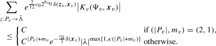 (3.3.37)
 -
If \(v\in S_{v_0}^*\) is an endpoint of type
 and
\(h_v = h_{v_0}+1\), then
\(K_v=0\) unless
\((|P_v|,\Vert {\varvec{D}}_v\Vert _1,m_v)=(2,p,1)\) with
\(p=0,1\), in which case
\(K_{v}(\Psi _v, {\varvec{x}}_v)=D_E ^{(h_{v_0})}(\Psi _v,{\varvec{x}}_v)\), with
\({\varvec{x}}_v=x_v\) consisting of a single point, so that
$$\begin{aligned} \begin{aligned}&\sum _{z: P_v \rightarrow {\bar{\Lambda }}}e^{\frac{7}{12}{c_0} 2^{h_{v_0}} \delta _E ({\varvec{z}}_v,x_v)}\big | K_v(\Psi _v,x_v)\big | \le \Vert (D_E ^{(h_{v_0})})_{2,\Vert {\varvec{D}}_v\Vert _1,1}(x_v)\Vert _{(E ;\frac{7}{12}{c_0}2^{h_{v_0}})}\\&\le e^{-\frac{c_0}{12}2^{h_v}\delta _E (x_v)} \Vert (D_E ^{(h_{v_0})})_{2,\Vert {\varvec{D}}_v\Vert _1,1}(x_v)\Vert _{(E ;\frac{3}{8}{c_0}2^{h_{v}})}. \end{aligned} \end{aligned}$$(3.3.38)
and
\(h_v = h_{v_0}+1\), then
\(K_v=0\) unless
\((|P_v|,\Vert {\varvec{D}}_v\Vert _1,m_v)=(2,p,1)\) with
\(p=0,1\), in which case
\(K_{v}(\Psi _v, {\varvec{x}}_v)=D_E ^{(h_{v_0})}(\Psi _v,{\varvec{x}}_v)\), with
\({\varvec{x}}_v=x_v\) consisting of a single point, so that
$$\begin{aligned} \begin{aligned}&\sum _{z: P_v \rightarrow {\bar{\Lambda }}}e^{\frac{7}{12}{c_0} 2^{h_{v_0}} \delta _E ({\varvec{z}}_v,x_v)}\big | K_v(\Psi _v,x_v)\big | \le \Vert (D_E ^{(h_{v_0})})_{2,\Vert {\varvec{D}}_v\Vert _1,1}(x_v)\Vert _{(E ;\frac{7}{12}{c_0}2^{h_{v_0}})}\\&\le e^{-\frac{c_0}{12}2^{h_v}\delta _E (x_v)} \Vert (D_E ^{(h_{v_0})})_{2,\Vert {\varvec{D}}_v\Vert _1,1}(x_v)\Vert _{(E ;\frac{3}{8}{c_0}2^{h_{v}})}. \end{aligned} \end{aligned}$$(3.3.38) -
If \(v\in S_{v_0}^*\) is an endpoint of type
 and
\(h_v = 2\), then
\(K_{v}(\Psi _v, {\varvec{x}}_v)=(B^{(1)}_E +{\mathcal {E}} B_B ^{(1)})(\Psi _v, {\varvec{x}}_v)\), so that
$$\begin{aligned} \begin{aligned}&\sum _{z: P_v \rightarrow {\bar{\Lambda }}}e^{\frac{7c_0}{12} 2^{h_{v_0}} \delta _E ({\varvec{z}}_v,{\varvec{x}}_v)}\big | K_v(\Psi _v,{\varvec{x}}_v)\big |\le e^{-\frac{c_0}{3}\delta _E ({\varvec{x}}_v)} \big (\delta _{\Vert {\varvec{D}}_v\Vert _1,0}\Vert (B^{(1)}_E )_{(|P_v|,0,m_v)}\Vert _{(E ;c_0)}\\&\quad + \delta _{|P_v|,2}\delta _{m_v,1}\mathbbm {1}(\Vert {\varvec{D}}_v\Vert _1\le 1)\max _{p=0,1}\Vert ({\mathcal {E}} B_B ^{(1)})_{(2,p,1)}\Vert _{(E ;c_0)}\big ), \end{aligned} \end{aligned}$$(3.3.39)
and
\(h_v = 2\), then
\(K_{v}(\Psi _v, {\varvec{x}}_v)=(B^{(1)}_E +{\mathcal {E}} B_B ^{(1)})(\Psi _v, {\varvec{x}}_v)\), so that
$$\begin{aligned} \begin{aligned}&\sum _{z: P_v \rightarrow {\bar{\Lambda }}}e^{\frac{7c_0}{12} 2^{h_{v_0}} \delta _E ({\varvec{z}}_v,{\varvec{x}}_v)}\big | K_v(\Psi _v,{\varvec{x}}_v)\big |\le e^{-\frac{c_0}{3}\delta _E ({\varvec{x}}_v)} \big (\delta _{\Vert {\varvec{D}}_v\Vert _1,0}\Vert (B^{(1)}_E )_{(|P_v|,0,m_v)}\Vert _{(E ;c_0)}\\&\quad + \delta _{|P_v|,2}\delta _{m_v,1}\mathbbm {1}(\Vert {\varvec{D}}_v\Vert _1\le 1)\max _{p=0,1}\Vert ({\mathcal {E}} B_B ^{(1)})_{(2,p,1)}\Vert _{(E ;c_0)}\big ), \end{aligned} \end{aligned}$$(3.3.39)where we used the fact that, by definition, \((B^{(1)}_E )_{(n,p,m)}\) vanishes for \(p=1\), and that, by Remark 3.10, \(({\mathcal {E}} B_B ^{(1)})_{(n,p,m)}\) vanishes unless \((n,p,m)\in \{(2,0,1), (2,1,1)\}\). Now, using (2.2.14) and (2.2.15), \(\Vert (B^{(1)}_E )_{n,0,m}\Vert _{(E ;c_0)}\) can be bounded from above by C, if \((n,m)=(2,1)\), and by \(C^{n+m}|\lambda |^{\max \{1,\kappa (n+m)\}}\), otherwise. In conclusion,
 (3.3.40)
 and
and
 and
and

 and
and
 and
and

Putting things together, we find

Now, the factors associated with the vertices \(v\in S_{v_0}{\setminus } S_{v_0^*}\) that are not endpoints are bounded as in Proposition 3.17. For the factors associated with the vertices \(v\in S_{v_0^*}\) that are not endpoints, we iterate the bound, and we continue to do so until we are left only with endpoints, or with vertices in \(V_0(\tau )\) with \(m_v=0\). By doing so, we obtain the desired bound, (3.3.31). \(\square \)
Next, we rearrange the bounds in Propositions 3.17 and 3.19 in a different form, more suitable for summing over GN trees and their labels, and for deriving the desired dimensional bounds on the multipoint energy correlations, to be discussed in Sect. 4 below. The result is summarized in the following proposition.
Proposition 3.23
Under the same assumptions as Propositions 3.17 and 3.19,

where \(d(P_v,{\varvec{D}}_v,m_v,E_v)=2-\frac{|P_v|}{2}-\Vert {\varvec{D}}_v\Vert _1-m_v-E_v\delta _{m_v,0}\) is the scaling dimension of v, see (3.2.24).
Remark 3.24
As discussed in Remark 3.13, the scaling dimension \(d(P_v,{\varvec{D}}_v,m_v,E_v)\) is negative (more precisely, it is \(\le -1\)) for all the allowed values of \(P_v,{\varvec{D}}_v,m_v,E_v\), with the only exception of the case \(|P_v|=2\), \({\varvec{D}}_v=\textbf{0}\) and \(m_v=E_v=1\), in which case it vanishes. A step-by-step repetition of the proof of [AGG22, Lemma 4.8] immediately implies that the sum over GN trees, restricted to allowed labels such that \((|P_v|,\Vert {\varvec{D}}_v\Vert _1,m_v,E_v)\ne (2,0,1,1)\) for all the vertices in \(V_0(\tau )\cup \{v\in V_e(\tau ): h_{v'}<h_v-1\}\), is convergent, uniformly in the scale of the root. In particular, let us state the resulting bound on the GN tree expansion for \((B_\infty ^{(h)})_{2,p,1}\), which will be used in the next section in order to bound \(Z_{j,h}, D_E ^{(h)}\) and \({\mathcal {E}} B_B ^{(1)}\): for \(h\le 0\), \(p\in \{0,1,2\}\), and (say) \(\theta =3/4\):
provided that
\(|\lambda |\) is sufficiently small (here the
\(*\) on the sum indicates, as usual, the constraint that
\(v_0=v_0(\tau )\) is dotted; in the present situation, this implies that
\(\tau \) has at least one endpoint of type
 ). Contrary to the trees contributing to
\((B_\infty ^{(h)})_{2,p,1}\) (or, more generally, to the bulk part of the effective source term,
\(B_B ^{(h)}\)), trees contributing to the edge part of the effective source term,
\(B_E ^{(h)}\), will, in general, contain vertices with
\((|P_v|,\Vert {\varvec{D}}_v\Vert _1,m_v,E_v)=(2,0,1,1)\), for which the scaling dimension vanishes; the presence of such vertices has a significant impact on the proof of convergence of the sum over GN trees for the multipoint correlation functions, to be discussed in Sect. 4 and in “Appendix C” below.
). Contrary to the trees contributing to
\((B_\infty ^{(h)})_{2,p,1}\) (or, more generally, to the bulk part of the effective source term,
\(B_B ^{(h)}\)), trees contributing to the edge part of the effective source term,
\(B_E ^{(h)}\), will, in general, contain vertices with
\((|P_v|,\Vert {\varvec{D}}_v\Vert _1,m_v,E_v)=(2,0,1,1)\), for which the scaling dimension vanishes; the presence of such vertices has a significant impact on the proof of convergence of the sum over GN trees for the multipoint correlation functions, to be discussed in Sect. 4 and in “Appendix C” below.
Proof
We start from (3.3.13) and (3.3.31). Recalling that \(R_v=\Vert {\varvec{D}}_v\Vert _1-\sum _{w\in S_v}\Vert {\varvec{D}}_w\big |_{P_v}\Vert _1\), and using [AGG22, Eq. (4.4.23)] and the analogue of [AGG22, (4.4.24)], we get

where \(d(P_v,{\varvec{D}}_v)=2-\frac{|P_v|}{2}-\Vert {\varvec{D}}_v\Vert _1\). If we now use the identity
and note that, for any \(v\in V_e(\tau )\) such that \((|P_v|,m_v)=(2,1)\) one has \(2^{-h_v d(P_v,{\varvec{D}}_v)}=2^{h_v\Vert {\varvec{D}}_v\Vert _1}2^{-h_vm_v}\), after rearranging the resulting factors, we get (3.3.41). \(\square \)
3.4 Beta function equation for \(Z_{j,h}\) and bounds on \(D_E ^{(h)}\), \({\mathcal {E}} B_B ^{(1)}\)
In this section we bound the effective vertex renormalizations \(Z_{j,h}\), with \(j=1,2\) and \(h\le 0\), and the kernels \(D_E ^{(h)}\), \({\mathcal {E}} B_B ^{(1)}\) involved in the definition of \(\tilde{Z}_{h_v-1}(E_v,\Vert {\varvec{D}}_v\Vert _1,x_v)\) in (3.3.32). The bound the effective vertex renormalizations is based on the control of their flow equation, known as the ‘beta function equation’ in the RG jargon, and is discussed in Sect. 3.4.1. The bounds on \(D_E ^{(h)}\) and \({\mathcal {E}} B_B ^{(1)}\) follow from an adaptation of “Appendix A”, and are discussed in Sect. 3.4.2.
3.4.1 Beta function equation for \(Z_{j,h}\).
The definition of the effective vertex renormalizations \(Z_{1,h}\) and \(Z_{2,h}\), see (3.1.48), combined with the GN tree expansion for the infinite volume effective potentials, see (3.2.6), implies the following equation, for all \(h\le 0\):
(recall
\(\Lambda _\infty := \mathbb {Z}^2\)). Note that the trees contributing to (3.4.1) have exactly one endpoint of type
 , and all the others (if any) of type
 or
or
 . Note also that sum over
\(\tau \) in (3.4.1) is absolutely convergent, with the contribution from the trees with
\(v_0\) dotted bounded as in (3.3.42). The case in which
\(v_0\) is not dotted corresponds to the contribution from the ‘trivial’ tree with exactly one endpoint (which is, therefore, of type
. Note also that sum over
\(\tau \) in (3.4.1) is absolutely convergent, with the contribution from the trees with
\(v_0\) dotted bounded as in (3.3.42). The case in which
\(v_0\) is not dotted corresponds to the contribution from the ‘trivial’ tree with exactly one endpoint (which is, therefore, of type
 ) on scale
\(h_v=h+2\) (in fact, if
\(h<0\), the contribution to (3.4.1) from the tree with exactly one endpoint v on scale
\(h_v=2\) and
\(v_0\) not dotted vanishes, because
\(\mathcal {L}_\infty (\mathcal {R}_\infty B^{(1)}_\infty )=0\), by the definition of
\(\mathcal {L}_\infty \) and
\(\mathcal {R}_\infty \)); moreover, the contribution from such a trivial tree equals
\(Z_{j,h+1}\), if
\(h<0\), and
\(4(\mathcal {L}_\infty B_\infty ^{(1)})_{2,0,1}(((+,-),{\varvec{0}},{\varvec{0}}),{{\hat{e}}}_j/2)\), if
\(h=0\).
) on scale
\(h_v=h+2\) (in fact, if
\(h<0\), the contribution to (3.4.1) from the tree with exactly one endpoint v on scale
\(h_v=2\) and
\(v_0\) not dotted vanishes, because
\(\mathcal {L}_\infty (\mathcal {R}_\infty B^{(1)}_\infty )=0\), by the definition of
\(\mathcal {L}_\infty \) and
\(\mathcal {R}_\infty \)); moreover, the contribution from such a trivial tree equals
\(Z_{j,h+1}\), if
\(h<0\), and
\(4(\mathcal {L}_\infty B_\infty ^{(1)})_{2,0,1}(((+,-),{\varvec{0}},{\varvec{0}}),{{\hat{e}}}_j/2)\), if
\(h=0\).
Thanks to these considerations, recalling also the fact that \(W_\infty ^{(1)}\) is analytic in \(\lambda \), see the comments after (2.2.19), and the bound on the norm of \(W_\infty ^{(1)}\) following from (2.2.8), (2.2.10) and following discussion, we find that, if \(h=0\), then \(Z_{j,0}\), with \(j=1,2\), are analytic in \(\lambda \), and bounded as \(|Z_{j,0}|\le C_0\) for all \(|\lambda |\le \lambda _0\) and some \(C_0>0\). More explicitly, recalling the definition of \(B_\infty ^{(1)}\) following from (2.2.18) and (2.2.5), the bound (2.2.8), and the facts that \(Z=1+O(\lambda )\), \(t_1^*-t_1=O(\lambda )\) and \(t_2^*-t_2=O(\lambda )\) with \(t_2^*=(1-t_1^*)/(1+t_1^*)\) (see Remark 3.9), after a straightforward computation we find that
with
If \(h<0\), distinguishing the contribution from the trivial tree with one endpoint on scale \(h_v=2\) from the rest, we can write
where the beta function \(B^j_{h+1}\) is given by the analogue of the right side of (3.4.1), modulo the constraint that trees contributing to \(B^j_{h+1}\) must have \(v_0\) dotted. Thanks to (3.3.42),
for \(\theta =3/4\). Equations (3.4.4) and (3.4.5), in combination with the absolute convergence of the expansion for \(B^j_{h+1}\) and the analyticity of \(W_\infty ^{(1)}\), imply that \(\{Z_{j,h}\}_{h\le 0}\), with \(j=1,2\), are two Cauchy sequences, whose elements are real analytic in \(\lambda \) for \(|\lambda |\le \lambda _0\). We let \(Z_{j,-\infty }=Z_{j,-\infty }(\lambda )=Z^*_j+O(\lambda )\) be the limit as \(h\rightarrow -\infty \) of \(Z_{j,h}\), which is also real analytic in \(\lambda \). Note also that, for \(\theta =3/4\) (say),
3.4.2 Bounds on \(D_E ^{(h)}\) and \({\mathcal {E}} B_B ^{(1)}\).
In this subsection we derive bounds on \(\Vert (D_E ^{(h)})_{2,p,1}(x)\Vert _{(E ;\frac{3}{4}c_02^h)}\) and \(\Vert (\mathcal E B_B ^{(1)})_{2,p,1}(x)\Vert _{(E ;c_0)}\), with \(p=0,1\), which are the norms entering the definition (3.3.32). Let us first consider \((D_E ^{(h)})_{2,p,1}\). Recall that, by the definition (3.2.18), \(D_E ^{(h)}=\sum _{k=h}^0 \mathcal {E}{{\tilde{B}}}_B ^{(k)}\), with
with \(I_\Lambda \) the kernel in (3.1.3), so that
In order to bound the norm of \({\mathcal {E}} {{\tilde{B}}}_{\text {B}}^{(k)}\), we proceed in a way analogous to “Appendix A”. Recall the definitions of \(\mathcal {L}_B \) and \(\mathcal {R}_B \) in (3.1.30)–(3.1.31), from which it follows, in particular, that \(({\mathcal {E}} \tilde{B}_{\text {B}}^{(k)})_{2,0,1}=((\mathcal {L}_B \tilde{B}_B ^{(k)})_{2,0,1})_E =(\mathcal {A}({\widetilde{\mathcal {L}}}({{\tilde{B}}}_B ^{(k)})_{2,0,1}))_E \) and \(({\mathcal {E}} \tilde{B}_{\text {B}}^{(k)})_{2,1,1}=((\mathcal {R}_B \tilde{B}_B ^{(k)})_{2,1,1})_E \) \(=(\mathcal {A}({\widetilde{\mathcal {R}}}{{\tilde{B}}}_B ^{(k)})_{2,1,1})_E \) (in writing the last identity, we used the fact that \((({\tilde{B}}_B ^{(k)})_{2,1,1})_E =0\), because it is the edge part of the bulk part of a kernel). From these formulas and the definition of \({\widetilde{\mathcal {R}}}\) in (3.1.32), it is apparent that \(({\mathcal {E}} \tilde{B}_{\text {B}}^{(k)})_{2,p,1}\) with \(p=0,1\) only depends on \((\tilde{B}_\infty ^{(k)})_{2,0,1}\), which, in view of (3.3.42) and the boundedness of \(Z_{j,h}\), see (3.4.6) and preceding lines, satisfies
We start with bounding the edge norm of \(({\mathcal {E}} \tilde{B}_{\text {B}}^{(k)})_{2,0,1}=(\mathcal {A}({\widetilde{\mathcal {L}}}(\tilde{B}_B ^{(k)})_{2,0,1}))_E \), which satisfies
with
the terms in the first sum on the right-hand-side are entirely cancelled by a corresponding set of terms in the second sum, leaving only those for which \({{\,\textrm{diam}\,}}_1({\varvec{y}}, x) > L/3\) or \(y_j\notin \Lambda \) for j equal either to 1 or 2, and for these remaining terms we have \(\delta ({\varvec{y}}, x) \ge \delta _E ({\varvec{z}}, x)\). As a result, for any \(\kappa ,\epsilon >0\),
that is, recalling the definition (3.1.41) of the edge norm,
where the norm in the right side is the infinite volume analogue of (3.1.40).
Next, we bound the edge norm of \(({\mathcal {E}} \tilde{B}_{\text {B}}^{(k)})_{2,1,1}=(\mathcal {A}({\widetilde{\mathcal {R}}}\tilde{B}_B ^{(k)})_{2,1,1})_E \), where, recalling the defintion of \({\widetilde{\mathcal {R}}}\) in (3.1.32),
where the interpolation path \({{\,\textrm{INT}\,}}\) in the last term in the right side is the infinite volume analogue of the one defined after (3.1.32); the construction of \({{\,\textrm{INT}\,}}_x\) is such that the first sum on the right hand side is over an empty set whenever either of the indicator functions before the second sum vanish, so again the first sum cancels all terms of the second sum which do not satisfy \(\delta ({\varvec{y}},x) \ge \delta _E ({\varvec{z}},x)\), giving, for any \(\kappa ,\epsilon >0\),
(for the last inequality, proceed analogously to [AGG22, Equations (4.2.26) to (4.2.28)]). In conclusion,
Putting things together, choosing \(\kappa =\frac{3}{4}c_02^k\) and \(\kappa +2\epsilon =c_02^{k}\), and using (3.4.8), we find, for \(p=0,1\),
Summing over k from h to 0, and bounding \(2^{-pk}\le 2^{-ph}\), we find
Similar considerations, in combination with the norm bound on \(B_\infty ^{(1)}\), which follows from the infinite volume analogues of (2.2.8) and (2.2.10), imply that
Summarizing, using the bounds of this subsection and recalling the definition (3.3.32) of \({{\tilde{Z}}}_{h_v-1}(E_v,\) \(|{\varvec{D}}_v\Vert _1,x_v)\), we have that the combination \(2^{h\Vert {\varvec{D}}_v\Vert _1}{{\tilde{Z}}}_{h_v-1}(E_v,|{\varvec{D}}_v\Vert _1,x_v)\) entering (3.3.43) satisfies
4 Correlation Functions
Recall that the truncated energy correlation functions of \(\epsilon _{x_1}, \ldots , \epsilon _{x_m}\), with \({\varvec{x}}=(x_1,\ldots ,\) \(x_m)\) an m-tuple consisting of \(m\ge 2\) distinct edges (or, equivalently, of edge midpoints) in \({\mathfrak {B}}_\Lambda \), can be computed as the derivative of \(\log \Xi _\Lambda ({\varvec{A}})\) with respect to \(A_{x_1},\ldots , A_{x_m}\) at \({\varvec{A}}={\varvec{0}}\); and that \(\Xi _\Lambda ({\varvec{A}})\) is given by (3.13), with \(\mathcal W^{(1)}({\varvec{A}})\equiv {\mathcal {W}}({\varvec{A}})=\sum _{{\varvec{x}}\in \mathcal {X}_\Lambda }w_\Lambda ({\varvec{x}}) {\varvec{A}}({\varvec{x}})\) as in (2.2.3), and \({\mathcal {W}}^{(h)}({\varvec{A}})\) with \(h\le 0\) as in (3.16), with the kernel \(w_\Lambda ^{(h)}\) expressed via the GN tree expansion (3.2.5). Consequently, we have arrived at
where \(t_1=\tanh (\beta _c(\lambda )J_1)\) and \(t_2=\tanh (\beta _c(\lambda ) J_2)\) are fixed as explained in Remark 3.9, the first sum in the right side runs over the m! permutations \(\pi \) of an m-tuple of distinct elements, and the \(*\) on the last sum in the right side indicates the constraint that the vertex \(v_0=v_0(\tau )\) is dotted. In (4.1), \(w_\Lambda \) comes from the transformation from spin to Grassmann variables summarized in Proposition 2.5, and vanishes at \(\lambda =0\); the remaining terms come from the iterative integration of the massive and massless Grassmann variables described in the previous section, and may or may not vanish at \(\lambda =0\), depending on the choice of \(\tau \).
Let \(m_1\) and \(m_2\) be the numbers of horizontal and vertical edges in \({\varvec{x}}\), respectively. We want to compare (4.1) with the rescaled, critical, non-interacting correlation function
where \(Z_{j,-\infty }=Z_{j,-\infty }(\lambda )\), with \(j=1,2\), is the limiting value of \(Z_{j,h}\) introduced in Sect. 3.4, and \(Z^*_j\) are defined as in (3.4.3). Recall that \(Z_{j,-\infty }/Z_j^*=1+O(\lambda )\) for \(j=1,2\). We intend to prove that the difference between (4.1) and (4.2) is bounded as the remainder term in Theorem 1.1, see (1.6). This will in fact prove Theorem 1.1.
Equation(4.2) can be computed by deriving with respect to \({\varvec{A}}\) the generating function
withFootnote 22
where, letting \(s^*_\omega (z):=\frac{1}{L}\sum _{k_1\in {\mathcal {D}}_L} \frac{e^{-ik_1z}}{1+t_1^*e^{\pm ik_1}}\) (and \({\mathcal {D}}_L\) defined as stated after (2.1.2)),
For later reference, we let \(B^qf _\Lambda \) be the \(\mathcal {A}\)-invariant kernel associated with (4.4), \(B^qf _\infty \) be its infinite volume limit, and \(B^qf _B , B^qf _E \) be its bulk and edge parts, respectively. In order to compare (4.1) with (4.2), it is convenient to rewrite the kernel \(w^qf _\Lambda ({\varvec{x}})\) in (4.3) as a sum over GN trees, in analogy with the (sum over scales of the) second line of (3.2.5), i.e.,
where
\(\mathcal {T}_{{\textrm{free}}}^{(h)}\) is the subset of
\(\mathcal {T}^{(h)}\) consisting of trees such that: (1) the endpoints are all either of type
 or of type
 and are all associated with a label
\(m_v=1\); (2) there are no endpoints v of type
and are all associated with a label
\(m_v=1\); (2) there are no endpoints v of type
 on scale
\(h_v<2\); (3) the vertices
\(v\in V_0'(\tau )\) have
\(|S_v|=|S_{v}^*|\ge 2\). Moreover, the
\(*\) on the sum over GN trees in the right side indicates the constraint that
\(v_0=v_0(\tau )\) is dotted. The definition of
\(w_\Lambda ^qf [\tau ]\) will be given momentarily. Recalling that (4.2) is the m-th derivative of (4.3) at the origin, we thus get
on scale
\(h_v<2\); (3) the vertices
\(v\in V_0'(\tau )\) have
\(|S_v|=|S_{v}^*|\ge 2\). Moreover, the
\(*\) on the sum over GN trees in the right side indicates the constraint that
\(v_0=v_0(\tau )\) is dotted. The definition of
\(w_\Lambda ^qf [\tau ]\) will be given momentarily. Recalling that (4.2) is the m-th derivative of (4.3) at the origin, we thus get
with \(W_\Lambda ^qf [\tau ,{\underline{P}},{\underline{T}}, {\underline{D}}]\) obtained via the same recursive definition as \(W_\Lambda [\tau ,{\underline{P}},{\underline{T}}, {\underline{D}}]\), see Sect. 3.2, up to the following differences:
-
If \(\tau \in \mathcal {T}^{(h)}_{\textrm{free}}\) and \(E_{v_0}=0\), then \(W_\Lambda ^qf [\tau ,{\underline{P}},{\underline{T}}, {\underline{D}}]\) is defined as in (3.2.11), with the function \(W_\infty \) in the right side replaced by \(W_\infty ^qf \); the latter is defined as described after (3.2.11), modulo the fact that \(K_{v,\infty }\) should be replaced by \(K_{v,\infty }^qf \), with \(K_{v,\infty }^qf =B^qf _\infty \) is \(h_{v_0}=1\), and

otherwise. Here: \(Z_{-\infty }\cdot F^A_\infty := Z_{1,-\infty } F_{1,\infty }+ Z_{2,-\infty } F_{2,\infty }\), with \(F_{j,\infty }\) the infinite volume analogue of \(F_{j,B }\), see (3.1.47) and preceding lines, and \({{\overline{W}}}^qf _\infty \) is defined recursively in a way analogous to \({{\overline{W}}}_\infty \).
-
If \(\tau \in \mathcal {T}^{(h)}_{\textrm{free}}\) and \(E_{v_0}=1\), then \(W_\Lambda ^qf [\tau ,{\underline{P}},{\underline{T}}, {\underline{D}}]\) is defined as in items (2) and (3) of Sect. 3.2, see (3.2.12) and following paragraphs, modulo the fact that \(K_v\) must be replaced by \(K_{v}^qf \), where, if \(h_{v_0}=1\), then
 , while, if
\(h_{v_0}<1\), then
, while, if
\(h_{v_0}<1\), then


 , while, if

The proof that the kernel \(w^qf _\Lambda \) of \(W^qf ({\varvec{A}})\) can be computed via the GN tree expansion (4.6), (4.8), is analogous to (and simpler than) the one in “Appendix B”, and left to the reader.
Remark 4.1
The condition that the trees contributing to (4.6) have no endpoints v of type
 on scale
\(h_v<2\) is due to the following: the value
\(D_E ^{qf ;(h_v-1)}\), which would be naturally (by mimicking the proof in “Appendix B”) associated with such vertices, should be defined as
on scale
\(h_v<2\) is due to the following: the value
\(D_E ^{qf ;(h_v-1)}\), which would be naturally (by mimicking the proof in “Appendix B”) associated with such vertices, should be defined as
with the \(*\) on the sum indicating the constraint that \(v_0=v_0(\tau )\) is dotted. However, (4.9) is identically zero, because the constraint \(m_{v_0}=1\) is incompatible with the requirement that \(\tau \in \mathcal {T}_{\textrm{free}}^{(h)}\) and \(v_0\) is dotted, as the reader can easily convince herself.
Note that, due to the definitions above, the sum over \({\underline{P}}\) in the right side of (4.8) can be freely restricted to the set \(\mathcal {P}_{\textrm{free}}(\tau )\subset \mathcal {P}(\tau )\) for which \(|P_v|=2\) for all \(v\in V'(\tau )\): in fact, whenever \(|P_v|\ge 4\) for some \(v\in V'(\tau )\), \(W_\Lambda ^qf [\tau ,{\underline{P}},{\underline{T}}, {\underline{D}}]=0\). In particular \(B^qf \) vanishes when its argument has more than two field labels, whereas \(B^{(1)}\), which it replaces in these expresssions, includes terms with four or more Grassmann fields, which arise from the transformation from spin to Grassmann variables summarized in Proposition 2.5.
We now write
where the set \(\mathcal {P}_*(\tau )\) in the second sum in the last line is defined as

Note that for
\(\tau \in \mathcal {T}_{\textrm{free}}^{(h)}\),
\(\mathcal {P}^*(\tau )\) is nonempty because
 and
and
 endpoints on scale 2 include factors of
\(B^{(1)}_B \) or
\(B^{(1)}_E \) which, unlike
\(B^{\textrm{free}}\), are not restricted to arguments with only two Grassmann fields.
endpoints on scale 2 include factors of
\(B^{(1)}_B \) or
\(B^{(1)}_E \) which, unlike
\(B^{\textrm{free}}\), are not restricted to arguments with only two Grassmann fields.
We denote by \(R_1({\varvec{x}})\) and \(R_2({\varvec{x}})\) the contributions from the sums in the second and third lines, respectively, so that
The contribution from \(w_\Lambda \) can be bounded via (2.2.4), which implies
which is smaller than the right side of (1.6). We are left with the contributions from \(R_1\) and \(R_2\), which are discussed in the following two subsections.
4.1 The remainder term \(R_1\)
Recall that
For each term in the sum, we write the difference \(W_\Lambda [\tau ,{\underline{P}},{\underline{T}},{\underline{D}}]- W^qf _\Lambda [\tau ,{\underline{P}},{\underline{T}},{\underline{D}}]\) as a telescopic sum of m terms, each of which has one endpoint associated with the value \(K_v-K^qf _v\) or \(K_{v,\infty }-K^qf _{v,\infty }\). These differences can be rewritten and bounded as follows (we restrict our attention to trees with \(h_{v_0}<1\) and to \(K_v-K^qf _v\), the other cases, namely \(h_{v_0}=1\) and \(K_{v,\infty }-K^qf _{v,\infty }\), being analogous).
-
1.
If \(v\in V_e(\tau )\) is of type
 and
\(h_v<2\), then
\(K_v-K^qf _v=(Z_{h_{v}-1}-Z_{-\infty })\cdot F^A_B \), so that
\(\Vert (K_v-K_v^qf )(x)\Vert _{0;h_v-1}\le C|\lambda |2^{\theta h_v}\), see (3.4.6).
and
\(h_v<2\), then
\(K_v-K^qf _v=(Z_{h_{v}-1}-Z_{-\infty })\cdot F^A_B \), so that
\(\Vert (K_v-K_v^qf )(x)\Vert _{0;h_v-1}\le C|\lambda |2^{\theta h_v}\), see (3.4.6). -
2.
If \(v\in V_e(\tau )\) is of type
 and
\(h_v=2\), then
\(K_v-K^qf _v=\big (\mathcal {R}_B (B^{(1)}_B -B^qf _B )_{2,0,1}\big )_{B }\), where
\((B^{(1)}_B -B^qf _B )_{2,0,1}=(Z^{-1}B^{{\textrm{free}}}_B -B^qf _B )_{2,0,1}+Z^{-1}(W^\textrm{int}_B )_{2,0,1}\), see (2.2.6) and following paragraphs for the definitions of the kernels
\(B^{{\textrm{free}}}_\Lambda \),
\(W^\textrm{int}_\Lambda \) and of their bulk counterparts. By the very definitions of
\(B^{{\textrm{free}}}_B \) and
\(B^qf _B \) and the facts that
\(Z-1=O(\lambda )\),
\(t_1-t^*_1=O(\lambda )\),
\(t_2-t_2^*=O(\lambda )\) (see Remark 3.9) and
\(Z_{j,-\infty }/Z_j^*-1=O(\lambda )\), we find that
\(\Vert (Z^{-1}B^{{\textrm{free}}}_B -B^qf _B )_{2,0,1}(x)\Vert _{(2c_0)}\le C|\lambda |\), with
\(c_0\) the same constant as in Proposition 2.5. Moreover, by using (2.2.8),
\(\Vert (W^\textrm{int}_B )_{2,0,1}(x)\Vert _{(2c_0)}\le C|\lambda |\). Therefore, using also (3.1.38), we find that, for any
\(c'<2c_0\),
\(\Vert (K_v-K_v^qf )(x)\Vert _{(c')}\le C|\lambda |/(2c_0-c')\).
and
\(h_v=2\), then
\(K_v-K^qf _v=\big (\mathcal {R}_B (B^{(1)}_B -B^qf _B )_{2,0,1}\big )_{B }\), where
\((B^{(1)}_B -B^qf _B )_{2,0,1}=(Z^{-1}B^{{\textrm{free}}}_B -B^qf _B )_{2,0,1}+Z^{-1}(W^\textrm{int}_B )_{2,0,1}\), see (2.2.6) and following paragraphs for the definitions of the kernels
\(B^{{\textrm{free}}}_\Lambda \),
\(W^\textrm{int}_\Lambda \) and of their bulk counterparts. By the very definitions of
\(B^{{\textrm{free}}}_B \) and
\(B^qf _B \) and the facts that
\(Z-1=O(\lambda )\),
\(t_1-t^*_1=O(\lambda )\),
\(t_2-t_2^*=O(\lambda )\) (see Remark 3.9) and
\(Z_{j,-\infty }/Z_j^*-1=O(\lambda )\), we find that
\(\Vert (Z^{-1}B^{{\textrm{free}}}_B -B^qf _B )_{2,0,1}(x)\Vert _{(2c_0)}\le C|\lambda |\), with
\(c_0\) the same constant as in Proposition 2.5. Moreover, by using (2.2.8),
\(\Vert (W^\textrm{int}_B )_{2,0,1}(x)\Vert _{(2c_0)}\le C|\lambda |\). Therefore, using also (3.1.38), we find that, for any
\(c'<2c_0\),
\(\Vert (K_v-K_v^qf )(x)\Vert _{(c')}\le C|\lambda |/(2c_0-c')\). -
3.
If \(v\in V_e(\tau )\) is of type
 and
\(h_v=2\), then
\(K_v-K^qf _v=(B^{(1)}_E -B^qf _E )_{2,0,1}+\sum _{p=0}^1({\mathcal {E}} B^{(1)}_B -{\mathcal {E}} B^qf _B )_{2,p,1}\), where, similarly to the decomposition used in the previous item, we write
\((B^{(1)}_E -B^qf _E )_{2,0,1}=(Z^{-1}B^{{\textrm{free}}}_E -B^qf _E )_{2,0,1}+Z^{-1}(W^\textrm{int}_E )_{2,0,1}\) and
\(({\mathcal {E}} B^{(1)}_B -{\mathcal {E}} B^qf _B )_{2,p,1}=(Z^{-1}{\mathcal {E}} B^{{\textrm{free}}}_B -{\mathcal {E}} B^qf _E )_{2,p,1}+Z^{-1}({\mathcal {E}} W^\textrm{int}_E )_{2,p,1}\). By the same considerations as in the previous item and the bounds (2.2.14), (2.2.15), we find that, for any
\(c'<2c_0\),
$$\begin{aligned} \Vert (B^{(1)}_E -B^qf _E )_{2,0,1}(x)\Vert _{(E ;c')}\le C|\lambda | e^{-(2c_0-c')\delta _E (x)}. \end{aligned}$$
and
\(h_v=2\), then
\(K_v-K^qf _v=(B^{(1)}_E -B^qf _E )_{2,0,1}+\sum _{p=0}^1({\mathcal {E}} B^{(1)}_B -{\mathcal {E}} B^qf _B )_{2,p,1}\), where, similarly to the decomposition used in the previous item, we write
\((B^{(1)}_E -B^qf _E )_{2,0,1}=(Z^{-1}B^{{\textrm{free}}}_E -B^qf _E )_{2,0,1}+Z^{-1}(W^\textrm{int}_E )_{2,0,1}\) and
\(({\mathcal {E}} B^{(1)}_B -{\mathcal {E}} B^qf _B )_{2,p,1}=(Z^{-1}{\mathcal {E}} B^{{\textrm{free}}}_B -{\mathcal {E}} B^qf _E )_{2,p,1}+Z^{-1}({\mathcal {E}} W^\textrm{int}_E )_{2,p,1}\). By the same considerations as in the previous item and the bounds (2.2.14), (2.2.15), we find that, for any
\(c'<2c_0\),
$$\begin{aligned} \Vert (B^{(1)}_E -B^qf _E )_{2,0,1}(x)\Vert _{(E ;c')}\le C|\lambda | e^{-(2c_0-c')\delta _E (x)}. \end{aligned}$$Similarly, using also considerations analogous to those of Sect. 3.4.2, we find that, for any \(c'<2c_0\),
$$\begin{aligned} \Vert ({\mathcal {E}} B^{(1)}_B -{\mathcal {E}} B^qf _B )_{2,p,1}\Vert _{(E ;c')}\le C|\lambda |e^{-(c_0-c'/2)\delta _E (x)}/(2c_0-c'). \end{aligned}$$
 and
and
 and
and
 and
and
By using the definition of the norm \(\Vert \cdot \Vert _{E_{v_0};h_{v_0}}\), we find, for \({\varvec{x}}_{v_0}\equiv {\varvec{x}}\),
where, in view of the previous considerations, of the proof of Proposition 3.19, and of Proposition 3.23, the norm of the difference \(W_\Lambda [\tau ,{\underline{P}},{\underline{T}},{\underline{D}}]- W^qf _\Lambda [\tau ,{\underline{P}},{\underline{T}},{\underline{D}}]\) in the second line is bounded as in (3.3.41) (with the factor in the last line simplifying to \(C^m\)Footnote 23) times an additional factor \(|\lambda | 2^{\theta h_M}\), which accounts for the bounds on \(K_v-K_v^qf \) discussed in items 1 to 3 above, where \(h_M=h_M(\tau ):= \max _{v\in V_e(\tau )}h_v\).
For \(\tau \in \mathcal {T}_{\textrm{free}}^{(h)}\) and \({\underline{P}}\in \mathcal {P}_{\textrm{free}}(\tau )\), all endpoints \(w\in V_e(\tau )\) are such that \(|P_w|=2\) and \(m_w=1\), which implies that \(|P_{v}|=2\) and \(m_v \ge 1\) for all \(v\in V'(\tau )\); therefore, recalling the definition \(d(P_v, {\varvec{D}}_v,m_v,E_v)=2-|P_v|/2-\Vert {\varvec{D}}_v\Vert _1-m_v-E_v\delta _{m_v,0}\) for all such vertices \(d(P_v,{\varvec{D}}_v,m_v,E_v)=1-m_v-\Vert {\varvec{D}}_v\Vert _1\). Noting also \(|P_{v_0}|=0\) (so that \(d(P_{v_0}, {\varvec{D}}_{v_0},m_{v_0},E_{v_0})=2-m\)), we find
This equation is analogous to [GGM12, Eq. (4.5)]. If we now plug (4.1.2) into (4.1.1) and sum over \({\underline{P}},{\underline{T}},{\underline{D}}\) (see the proof of [AGG22, Lemma 4.8] for additional details), we get
where the last two products should be interpreted as 1 if they run over an empty set, and the factors \(2^{h_{v'}}\) associated with the endpoints v with \(E_v=0\) and \(h_v=2\) come from the factors \(2^{-(h_v-h_{v'})\Vert {\varvec{D}}_v\Vert _1}\) in the second line of (4.1.2): recall, in fact, that, due to the action of the \(\mathcal {R}_B \) operator, the kernel associated with such endpoints is different from zero only if \(\Vert {\varvec{D}}_v\Vert _1=1\).
We now manipulate this expression further. Write the factors \(2^{2(|S_v|-1)h_v}\) as \(2^{(|S_v|-1)h_v}\cdot 2^{(|S_v|-1)h_v}\). Keep one of these factors on a side, and rewrite the product of the other as
By using the identity
which can be easily proved by induction, we can rewrite this product as
Plugging this into (4.1.3) and letting, for short, \(\delta _v:=\delta _{E_v}({\varvec{x}}_v)\), we find
This is the analogue of [GGM12, Eq. (4.13)]. Let \(\mathfrak d={\mathfrak {d}}({\varvec{x}})\) be the minimal pairwise distance between the points in \({\varvec{x}}\). Using the fact that, for any \(n>1\),
see [BCO04, Lemma 3.4], we can bound from below \(\delta _v\ge \frac{1}{2} (m_v-1){\mathfrak {d}}\ge \frac{1}{2} (|S_v|-1){\mathfrak {d}}\); we use this estimate in (4.1.5) for all vertices in \(V_0(\tau )\) such that \(v>v_0^*\), where \(v_0^*=v_0\), if \(|S_{v_0}|>1\), and \(v_0^*\) equal to the only element of \(S_{v_0}\), otherwise; for \(v\in \{v_0,v_0^*\}\) we use that \(\delta _{v}=\delta ({\varvec{x}})\ge \frac{1}{3}(\delta ({\varvec{x}})+(|S_v|-1){\mathfrak {d}})\). Next, in the sum over \(\tau \), we distinguish two cases: either \(\tau \) has all the endpoints on scales \(<2\), in which case \(2^{\theta h_M}=2^{\theta (h_{v^*}+1)}\) for some \(v^*\in V_0'(\tau )\), or it has at least one endpoint on scale 2, in which case, letting \({\mathfrak {d}}_\partial = {\mathfrak {d}}_\partial ({\varvec{x}})\) be the minimum of \(\delta _E (x)\) over the elements x of \({\varvec{x}}\), \(\Big (\prod _{v \in V_e(\tau )}^{E_v=0,\, h_v=2} 2^{h_{v'}}\Big )\,\Big (\prod _{v \in V_e(\tau )}^{E_v=1,\, h_v=2} e^{-\frac{c_0}{3}\delta _v}\Big )\le 2^{h_{v^*}}+e^{-\frac{c_0}{3}{\mathfrak {d}}_\partial }\) for some \(v^*\in V_0'(\tau )\). In view of these considerations, letting \(v^*\) be the vertex in \(V_0'(\tau )\) such that \(h_{v^*}=\max _{v\in V_0'(\tau )}\{h_v\}\), (4.1.5) implies that
where (I) is the term proportional to \(2^{\theta h_{v^*}}\), while (II) is the one proportional to \(e^{-\frac{c_0}{3}\mathfrak d_\partial }\). Term (I) is bounded exactly as described in [GGM12, Eqs. (4.13)–(4.17)]; by proceeding as discussed there, we find the analogue of [GGM12, Eq.(4.17)], namely
Term (II) is bounded via an analogous strategy. For completeness, let us describe it explicitly: we split the sum over trees \(\tau \) into a sum over the scale labels \(\{h_v\}_{v\in V(\tau )}\), and a sum over the remaining structure of the tree, its ‘skeleton’. For fixed skeleton, we sum over the scale labels \(h_v\), neglecting all the constraints but \(h_{v_0}=h+1\le h_{v_0^*}\). By summing \(2^{h_{v_0}-h_{v_0^*}}\) in the right side of (4.1.7) over \(h_{v_0}\equiv h+1\), for \(h_{v_0}\le h_{v_0^*}\), we get a factor \(\sum _{j\le 0}2^j=2\). Next, by summing \(e^{-\frac{c_0}{36}2^{h_{v_0^*}} (\delta ({\varvec{x}})+(|S_{v_0^*}|-1){\mathfrak {d}})} 2^{h_{v_0^*}|S_{v_0^*}|}\) over \(h_{v_0^*}\) we get a factor
where we used the fact that, for any \(\alpha ,\delta >0\),
Similarly, by summing \(2^{(|S_v|-1)h_v} e^{-\frac{c_0}{24}2^{h_v}(|S_v|-1){\mathfrak {d}}}\) over \(h_v\) we get a factor
Putting things together, and using the fact that the number of skeletons with m endpoints is bounded by (const.) \(^m\), see [GM01, Lemma A.1], we find that, up to a further redefinition of the constant C,
where the sup is over the choices of \(|S_v|\) compatible with the trees in \(\mathcal {T}^{(h)}_{\textrm{free}}\) with m endpoints, and in the second inequality we used the fact that \(|S_{v_0^*}|\ge 2\). By using the fact that \(\sum _{v\in V_0(\tau )}(|S_v|-1)=m-1\), see (4.1.4), we finally get
Combining (4.1.8) and (4.1.11), we obtain the desired bound on \(R_1({\varvec{x}})\),
4.2 The remainder term \(R_2\)
Let us now focus on
which, letting \({\varvec{x}}_{v_0}\equiv {\varvec{x}}\), we bound as
In view of Proposition 3.23, the norm of \(W_\Lambda [\tau ,{\underline{P}},{\underline{T}},{\underline{D}}]\) is bounded as in (3.3.41), with \({{\tilde{Z}}}_{h_v-1}(E_v,\) \(\Vert {\varvec{D}}_v\Vert _1,x_v)\) bounded as in (3.4.18), so that, after summing over \({\underline{T}}\) (using, in particular, [AGG22, Eq. (4.4.29)])
where, in the first product in the second line, \(d_v\) is a shorthand for \(d(P_v,{\varvec{D}}_v,m_v,E_v)\), and, in the products in the last line, \(**\) indicates the constraint that \((|P_v|,m_v)\ne (2,1)\), while \({*\!*\!*}\) indicates the constraint that \(m_v=E_v=1\) and \(h_v\le 1\) (which implies that \(|P_v|=2\)). Note that the restriction to \({\underline{P}} \in \mathcal {P}_*(\tau )\) implies that at least one of the two products in the last line runs over a non-empty set (and, as usual, whenever one of the products runs over the empty set, it should be interpreted as 1). Recall also the following properties of \(d_v\): for all the allowed choices of \(P_v, {\varvec{D}}_v, m_v, E_v\) in (4.2.3), \(d_v\le -1\), with the following exceptions:
-
1.
if \((|P_v|, \Vert {\varvec{D}}_v\Vert _1, m_v, E_v)=(2,0,1,1)\), then \(d_v=0\);
-
2.
if v is an endpoint such that \(h_v-h_{v'}=1\), in which case \(d_v\) may be equal to 0 (if \((|P_v|, \Vert {\varvec{D}}_v\Vert _1\), \(m_v, E_v){=}(4,0,0,0), (2,1,0,0), (2,0,0,1), (2,0,1,0), (2,0,1,1)\)), or to 1 (if \((|P_v|, \Vert {\varvec{D}}_v\Vert _1, m_v\), \(E_v){=}(2,0,0,0)\)).
Note, incidentally, that, from the definition of tree values, the choice \((|P_v|, \Vert {\varvec{D}}_v\Vert _1\), \(m_v, E_v)=(4,0,0,0)\) (corresponding to a vanishing scaling dimension) is not allowed; the choices (2, 1, 0, 0), (2, 0, 0, 1), (2, 0, 1, 0), (2, 0, 0, 0) (corresponding to scaling dimensions equal to 0 or 1) are allowed, but, as just remarked, they require \(h_{v'}=h_v-1\); the only allowed choice for which the scaling dimension is non-negative and \(h_{v'}\) may be smaller than \(h_v-1\) is \((|P_v|, \Vert {\varvec{D}}_v\Vert _1\), \(m_v, E_v)=(2,0,1,1)\).
The presence of cases for which \(d_v\ge 0\) means that the sum must be handled differently than in the otherwise similar sums considered in [AGG22, Proof of Lemma 4.8] (see Remark 3.24), since the corresponding factors \(2^{d_v(h_v-h_{v'})}\) are not exponentially small in \(h_v-h_{v'}\). Clearly, the second case listed above is not problematic, because \(h_v-h_{v'}=1\); in that case, if desired, the factors \(2^{d_v(h_v-h_{v'})}\) with \(d_v=0,1\) can be freely replaced by \(2^{-(h_{v}-h_{v'})}\), at the cost of a factor smaller than \(2^{2N_{4}}\); here \(N_{4}\) is the number of endpoints with \(|P_v|\le 4\), which can be reabsorbed in the factor \( C^{\sum _{v\in V_e(\tau )}|P_v|}\) in the right side of (4.2.3), up to a redefinition of C. To summarize, the bound (4.2.3) remains valid, up to a redefinition of the constant C, even if we replace the factors \(2^{d_v(h_v-h_{v'})}\) in the first product in the second line by the smaller factors \(2^{d_v'(h_v-h_{v'})}\), where

We now further manipulate (4.2.3) (or, better, its rewriting with
\(d_v\) replaced by
\(d_v'\)), by proceeding in a way similar to what it was done in [GGM12] after [GGM12, Eq.(4.20)]. We let
\(V_e^{A}(\tau )=\{v\in V_e(\tau ): \ m_v\ge 1\}\), and
\(\tau ^*(\tau )\) be the minimal subtree of
\(\tau \) containing
\(v_0\) and all the endpoints in
\(V_e^A(\tau )\). Our first step consists in ‘pruning’ the tree
\(\tau \) of the branches that are not in
\(\tau ^*(\tau )\). For this purpose, we make the following rearrangement. Let
\(\mathcal {T}^{*}_{h,h_0^*;m}\) be the set of labelled trees with endpoints all of type
 or
or
 ,
\(m_{v_0}=m\), no trivial vertices, dotted root
\(v_0\) on scale
\(h+1\), and with the leftmost branching point, which we denote by
\(v_0^*\), on scale
\(h_0^*\ge h+1\) (if
\(h_0^*=h+1\), then
\(v_0=v_0^*\), otherwise
\(v_0^*\) is the vertex immediately following
\(v_0\) on
\(\tau ^*\); if
\(\tau ^*\) has no branching points, then
\(h_0^*=2\) and
\(v_0^*\) is the only endpoint of
\(\tau ^*\)); ‘as usual’, the endpoints may be on scale 2 or smaller; however, if v is an endpoint on scale
\(h_v<2\), we do not assume that the vertex immediately preceding it on
\(\tau ^*\) is on scale
\(h_{v}-1\), we allow the case that
\(h_{v'}<h_v-1\). Given
\(\tau ^*\in \mathcal {T}^{*}_{h,h_0^*;m}\) and
\(v\in V_0(\tau ^*)\), we denote by
\(s^*_v\) the number of vertices immediately following v on
\(\tau ^*\) (note that, since by definition
\(\tau ^*\) does not have trivial vertices,
\(s^*_v>1\) for all
\(v\in V_0'(\tau ^*)\)),
,
\(m_{v_0}=m\), no trivial vertices, dotted root
\(v_0\) on scale
\(h+1\), and with the leftmost branching point, which we denote by
\(v_0^*\), on scale
\(h_0^*\ge h+1\) (if
\(h_0^*=h+1\), then
\(v_0=v_0^*\), otherwise
\(v_0^*\) is the vertex immediately following
\(v_0\) on
\(\tau ^*\); if
\(\tau ^*\) has no branching points, then
\(h_0^*=2\) and
\(v_0^*\) is the only endpoint of
\(\tau ^*\)); ‘as usual’, the endpoints may be on scale 2 or smaller; however, if v is an endpoint on scale
\(h_v<2\), we do not assume that the vertex immediately preceding it on
\(\tau ^*\) is on scale
\(h_{v}-1\), we allow the case that
\(h_{v'}<h_v-1\). Given
\(\tau ^*\in \mathcal {T}^{*}_{h,h_0^*;m}\) and
\(v\in V_0(\tau ^*)\), we denote by
\(s^*_v\) the number of vertices immediately following v on
\(\tau ^*\) (note that, since by definition
\(\tau ^*\) does not have trivial vertices,
\(s^*_v>1\) for all
\(v\in V_0'(\tau ^*)\)),
The idea is to rewrite the sum over \(\tau \) in (4.2.3) as a sum over \(\tau ^*\in \mathcal {T}^*_{h,h_0^*;m}\) times a sum over trees \(\tau \) compatible with \(\tau ^*\), i.e., such that \(\tau ^*(\tau )=\tau ^*\). Having done this, we will perform the sums in the following order: first we sum over \(\tau \) and \({\underline{P}}\) at \(\tau ^*\) fixed, and then over \(\tau ^*\).
Fix \(\theta =3/4\), as above, let \(\epsilon :=(1-\theta )/3\), and define
Using the definition of \(d_v'\) in (4.2.4) and of \(d_v=d_v(P_v,{\varvec{D}}_v,m_v,E_v)\) in (3.2.24), it is easy to check that
while \(d_v'={{\tilde{d}}}_v=0\), if \((|P_v|,\Vert {\varvec{D}}_v\Vert _1,m_v,E_v)= (2,0,1,1)\). We now: neglect the factor \(e^{-\frac{c_0}{2}2^{h_{v_0}}\delta _{E_{v_0}}({\varvec{x}})}\) in (4.2.3), since a comparable one is contained in the second product in the second line of (4.2.3), and, recalling that \(h_{v_0}=h+1\), we rearrange the result as follows:
where, given \(\tau ^*\in \mathcal {T}^*_{h,h_0^*;m}\), \(\mathcal {T}(\tau ^*)\) is the subset of trees in \(\mathcal {T}^{(h)}\) such that \(\tau ^*(\tau )=\tau ^*\). Equation(4.2.7) is the analogue of the un-numbered equation after [GGM12, Eq.(4.22)]. We now perform the sums in braces and, in analogy with [GGM12, Eq.(4.23)], we get
where \(h^*_M=h_M(\tau ^*)=\max \{h_v:\ v\in V_e(\tau ^*)\}\), \(\theta '=\theta -\epsilon /2\), and \({\mathfrak {d}}_\partial =\mathfrak d_\partial ({\varvec{x}})=\min _{v\in V_e(\tau ^*)}\delta _E (x_v)\). The proof of (4.2.8) is given in “Appendix C”, and is one of the important novelties of the current work, as compared to [GGM12]. Of course, the new source of difficulty, as compared to the proof of [GGM12, Eq.(4.23)], is the possible presence of vertices such that \(d_v'={{\tilde{d}}}_v=0\), for which the factor \(2^{(d_v'-{{\tilde{d}}}_v)(h_v-h_{v'})}\) equals 1, rather then being exponentially small in \((h_v-h_{v'})\) and in \(|P_v|\).
Plugging (4.2.8) in (4.2.7) gives, letting again \(\delta _{E_v}({\varvec{x}}_v)\equiv \delta _v\):
where in the second inequality we used the definition of \(\tilde{d}_v\) explicitly, and we distinguished the terms in the products associated with \(v_0^*\), from those associated with the vertices in \(V_0(\tau ^*)\setminus \{v_0^*\}\), from those associated with the endpoints.
In the last identity in (4.2.9), the contributions denoted by (I), (II), (III) are defined as follows. Consider first the contribution to the right side of (4.2.9) proportional to \(2^{\theta ' h^*_M}\), and let \({{\bar{v}}}\) be the endpoint that realizes the maximum in the definition of \(h^*_M\), i.e., \(h^*_M=h_{{{\bar{v}}}}\). We further distinguish two cases: (1) \((E_{{{\bar{v}}}},m_{{{\bar{v}}}})=(0,1)\) (which means that \({{\bar{v}}}\) is included in the product \(\prod _{v \in V_e(\tau ^*)}^{E_v=0,\, m_v=1} 2^{-\theta (h_v-h_{v'})}\)); (2) \((E_{{{\bar{v}}}},m_{\bar{v}})\ne (0,1)\) (which means that \({{\bar{v}}}\) is included in one of the two products in the last line of (4.2.9)). In terms of these definitions, we denote by (I) (resp. (II)) the contribution to the right side of (4.2.9) proportional to \(2^{\theta ' h^*_M}\) and associated with trees realizing case (1) (resp. (2)). Finally, we denote by (III) the contribution to the right side of (4.2.9) proportional to \({\mathfrak {d}}_\partial ^{-\theta }\).
The definition of (I) is completely analogous to [GGM12, Eq.(4.24)]; by proceeding as discussed there, we get the analogue of [GGM12, Eq.(4.33)], i.e.,
Let us now consider (II), which we manipulate as follows. First, we rewrite the product of the factors \(2^{(1+\epsilon -m_v)(h_v-h_{v'})}\) as
where \(s^{*,2}_v=|S^{*,2}_v|\), with \(S^{*,2}_v=S^*_v\cap V_0(\tau ^*)\), and \(m^{*,2}_v=\sum _{w\in S^{*,2}_v}m_w\). Recall the notation \(s^{*}_v=|S^*_v|\), where, since \(\tau ^*\) has no endpoints with \(m_v=0\), \(S^*_v\) is the same thing as \(S_v\), i.e., it is the set of vertices immediately following v on \(\tau ^*\). For later reference, we also let \(s^{*,1}_v=\{\)number of endpoints with \(m_v=1\) immediately following v on \(\tau ^*\}\), \(s^{*,>}_v=\{\)number of endpoints with \(m_v>1\) immediately following v on \(\tau ^*\}\), and \(m^{*,>}_v=m_v-s^{*,1}-m^{*,2}_v\) (note that \(m^{*,>}\) is the sum of \(m_w\) over the endpoints w with \(m_w>1\) immediately following v on \(\tau ^*\)). If we use (4.2.11) in (4.2.9) and we associate each factor \(2^{(m_v-1-\epsilon )h_{v'}}\) in the last product of (4.2.9) with the vertex \(v'\) immediately preceding the endpoint v with \(m_v>1\), we find:
where the label (II) on the sum indicates the constraint that the endpoint \({{\bar{v}}}\) such that \(h_{{{\bar{v}}}}=\max _{v\in V_e(\tau ^*)}h_v\) is such that \((E_{\bar{v}},m_{{{\bar{v}}}})\ne (0,1)\) (in particular, the second product in the second line is not empty), and
In order to bound (4.2.12) we proceed in a way similar to the one used to bound term (II) in (4.1.7). Recalling that \({\mathfrak {d}}\) is the minimal pairwise distance between the points in \({\varvec{x}}\) and that \({\mathfrak {d}}_\partial \) is the minimum of \(\delta _E (x)\) over the points x in \({\varvec{x}}\), we bound
Next, we bound \(\delta _v\) from below by \(\frac{1}{2}(m_v-1){\mathfrak {d}}\ge \frac{1}{2}(s_v-1){\mathfrak {d}}\) for all vertices of \(\tau ^*\) such that \(v>v_0^*\); for \(v=v_0^*\), we use \(\delta _{v_0^*}\ge \frac{1}{3}(\delta ({\varvec{x}})+(s_{v_0^*}-1){\mathfrak {d}})\). We perform the sum over \(\tau ^*\) by first summing over the scale labels, and then over the remaining structure (‘skeleton’) of the tree. By summing the factor \(2^{(h-h_0^*)(1-\epsilon )}\) over \(h<h_0^*\) with the other scales fixed, we get \(\sum _{j\le -1}2^{j(1-\epsilon )}\). By summing the factors \(2^{-\theta (h_v-h_{v'})}\) over the scale labels of the endpoints with \(m_v=1\) and \(E_v=0\) with the other scales fixed, we get a factor \(\sum _{k\ge 1}2^{-\theta k}\) for each such endpoint. By summing the factor \(2^{\alpha _{v_0^*} h_0^*} e^{-\frac{c_0}{36}2^{h_0^*}(\delta ({\varvec{x}})+(m-1){\mathfrak {d}}}\) over \(h_0^*\) we get \([{(\mathrm const.)}/(\delta ({\varvec{x}})+(m-1)\mathfrak d)]^{\alpha _{v_0^*}}\Gamma (\alpha _{v_0^*})\) (see (4.1.9)). Similarly, by summing the factors \(2^{\alpha _{v} h_v} e^{-\frac{c_0}{24}2^{h_0^*}(m_v-1){\mathfrak {d}}}\) over \(h_v\) we get \([(\mathrm{const.})/((m_v-1)\mathfrak d)]^{\alpha _{v}}\Gamma (\alpha _{v})\). Finally, using the fact that the number of skeletons with \(\le m\) endpoints is smaller than \((\mathrm{const.})^m\), we find the analogue of (4.1.10), namely
where the sup is over the trees \(\tau ^*\) involved in the sum in (4.2.12) (and, therefore, over the corresponding choices of \(s^*_v, s^{*,1}_v, m_v\)). By using the fact that \(s^*_{v_0^*}\ge 2\), that \(\sum _{v}(s^*_v-1)=N-1\), with \(N=N(\tau ^*)=|V_e(\tau ^*)|\), and that \(\sum _{v\in V_0(\tau )}s^{*,1}_v=m_1\), with \(m_1=m_1(\tau ^*)=\{\)number of endpoints of \(\tau ^*\) with \(m_v=1\}\), we get:
Each of the factors \(\frac{e^{-\frac{c_0}{12}(m_v-1)\mathfrak d}}{{\mathfrak {d}}^{1-\epsilon }}\) can be bounded from above by \(C^{m_v}{\mathfrak {d}}^{-m_v}\) for some constant \(C>0\), so that, in conclusion,
Finally, a repetition of the proof leading to (4.2.17) implies that, similarly,
Combining (4.2.17) and (4.2.18) with (4.2.10), we find that
Finally, plugging this bound, together with the analogous bound on \(R_1\), Eqs. (4.1.12), and (4.12), into (4.11), proves (1.6) and concludes the proof of the main result of this paper, Theorem 1.1.
Notes
This result was stated for pair interactions (of either sign) only, but the generalization to other finite-range interactions is straightforward.
More precisely, in [GGM12] the authors considered model (1.1) on a discrete torus \(\Lambda \) of side L and performed the following special scaling limit: first \(L\rightarrow \infty \) for \(\beta \ne \beta _c(\lambda )\), with \(\beta _c(\lambda )\) the critical inverse temperature of the interacting model; then \(\beta \rightarrow \beta _c(\lambda )\) and, simultaneously, after appropriate rescaling of the energy observable, lattice mesh to zero.
We use the convention that \({\mathbb {N}}\) is the set of positive integers, and \({\mathbb {N}}_0\) the set of non-negative integers. Compared to [AGG22], we do not assume here that L is even: the proof (both here and in [AGG22]) goes through without any significant modification, irrespective of the parity of L.
In the following we shall denote the components of \(z\in \Lambda \) by \((z)_1, (z)_2\), rather than by \(z_1,z_2\), in order to avoid confusion with the first two elements of an n-tuple \({\varvec{z}}\in \Lambda ^n\), for which we will use the notation \({\varvec{z}}=(z_1,\ldots , z_n)\).
\(\delta ({\varvec{z}})\) is the same as the so-called Steiner diameter of \({\varvec{z}}\). For n-ples of points in the plane, it is defined as \(\delta ({\varvec{z}}):=\min _{k\ge 0}\min _{{\varvec{z}}'\in (\mathbb R^2)^k}\min _{\tau \in \mathcal {T}({\varvec{z}},{\varvec{z}}')}L(\tau )\), where \(\mathcal {T}({\varvec{z}},{\varvec{z}}')\) is the set of all possible trees with vertices in the elements of the \((n+k)\)-tuple \({\varvec{z}}\oplus {\varvec{z}}'\equiv ({\varvec{z}},{\varvec{z}}')\), and \(L(\tau )\) is the tree length of \(\tau \), i.e., the sum of the Euclidean lengths of the edges of \(\tau \). For n-ples of points in the cylinder the definition is the same, provided the Euclidean distance in \({\mathbb {R}}^2\) is replaced by its analogue in the cylinder.
The generalization of Corollary 1.2 to the case of the half-plane concerns the scaling limit of the energy correlations computed in the following way: \(\lim _{a\rightarrow 0^+}\lim _{L,M\rightarrow \infty } { \left\langle \varepsilon _{l_1}^a(x_1) \cdots \varepsilon _{l_m}^a(x_m) \right\rangle }_{\lambda ,t_1(\lambda ),t_2(\lambda );\Lambda ^a}\), i.e., \(L,M\rightarrow \infty \) first, then \(a\rightarrow 0\); here, as usual, \(\Lambda ^a=a\Lambda \), with \(\Lambda \) the cylinder of sides L and M, and the limit \(L,M\rightarrow \infty \) is computed under the constraint that \(L/M\in K\). The uniformity in L, M of our bounds, valid as long as \(L/M\in K\), implies that the limit computed this way is the same as the limit of (1.11)–(1.12) as \(\ell _1,\ell _2\rightarrow \infty \), under the constraint that \(\ell _1/\ell _2\in K\).
Although there is no exact duality relating different boundary conditions for the model with \(\lambda \ne 0\), we expect that the non-integrable model with fixed, say \(+\), boundary conditions can be studied via a multiscale perturbation theory around a non-interacting model with renormalized, dressed, parameters and the same fixed boundary conditions. Such a reference non-interacting model is dual to its counterpart with open boundary conditions, and the main features of the expansion should be the same as for the open boundary conditions we consider here: in particular boundary terms should be irrelevant in this case as well. Consequently, duality between open and fixed boundary conditions should be an emergent property in the scaling limit of the interacting model.
An additional, less consequential, limitation is the non-uniformity of our result, as the aspect ratio of the cylinder tends to zero or infinity. We expect to be able to overcome this limitation easily, by studying the regime of infrared scales corresponding lengths larger than L but smaller than M, or viceversa, via a different multiscale scheme, taking into account the quasi-1D nature of the system at such scales. We decided not to do this explicitly in this paper, just in order to limit its length. We expect that such a refined scheme will allow us to prove the analogue of Theorem 1.1 and Corollary 1.2 without any restriction on the aspect ratio. In particular, the result of Corollary 1.2 would generalize to infinite cylindrical strips, and would allow us to check conformal covariance of the limit from the strip to the half-plane.
It is likely that an extension of these methods would ‘easily’ give non-optimal quantitative bounds [Che], but these would not suffice for our purposes.
The factor 2 in front of \(c_0\) at exponent is chosen for convenience and uniformity with later notations: in fact, the bare Grassmann action will be identified with the bare effective potential on scale \(h=1\), see (2.2.17), (3.1), and following equations; the factor 2 at exponent should be interpreted as being equal to \(2^h\), with scale index \(h=1\).
For instance, given \({\varvec{z}}=(z_1,\ldots , z_n)\in \Lambda ^n\), recalling that \((z_i)_1\in \{1,2,\ldots , L\}\) and \((z_i)_2\in \{1,2,\ldots , M\}\), we can let \({\varvec{z}}_\infty =(y_1,\ldots ,y_n)\) be the n-tuple of points of \({\mathbb {Z}}^2\) such that: (1) the vertical coordinates are the same as those of \({\varvec{z}}\), i.e., \((y_i)_2=(z_i)_2\), \(\forall i=1,\ldots , n\); (2) the horizontal coordinate of \(y_1\) is the same as \(z_1\), i.e., \((y_1)_1=(z_1)_1\); (3) all the other horizontal coordinates are the same modulo L, i.e., \((y_i)_1=(z_i)_1\) mod L, \(\forall i=2,\ldots , n\); (4) the specific values of \((y_i)_2\) for \(i\ge 2\) are chosen in such a way that the horizontal distances between the corresponding pairs in \({\varvec{z}}\) and \({\varvec{z}}_\infty \) are the same, if measured on the cylinder \(\Lambda \) or on \({\mathbb {Z}}^2\), respectively.
Actually, in order to define a convergent expansion, it is not necessary to split the effective source term \(\mathcal {B}^{(h)}(\phi ,{\varvec{A}} ):=\mathcal {V}^{(h)}(\phi , {\varvec{A}}) - \mathcal {V}^{(h)}(\phi , 0)\) into local plus irrelevant part, since this is not the source of any divergence. Nevertheless, in order to compute the scaling limit of the energy correlations, it is convenient to also decompose the effective source term into a local part plus a remainder, and we shall do so in Sect. 3.1 and following sections.
The running coupling constants used here and in [AGG22] are not strictly speaking equal to those of [GGM12] even in the isotropic case because of a number of changes in the quantities used to define them, most importantly the different decomposition of the propagators, but the general outline of the construction is the same.
On the basis of the general Wilsonian RG theory, the scaling dimension of a kernel describes the way in which it transforms under rescalings of the spatial coordinates and of the fields or, equivalently, under the action of the linearized Wilsonian RG transformation. On general grounds, for a kernel of order (n, p), it is equal to \(d-n\Delta _\phi -p\), where d is the spatial dimension, and \(\Delta _\phi \) the scaling dimension of the field \(\phi \), i.e., half the critical exponent of the two-point function of \(\phi \): \(\langle \phi _x\phi _y\rangle \sim |x-y|^{-2\Delta _\phi }\). In our case, \(d=2\) and \(\Delta _\phi =1/2\), which explains the expression \(2-n/2-p\) in (3.1.5).
If \({{\,\textrm{diam}\,}}_1(z,z')<L/2\), there is no ambiguity in the definition of such a shortest path. If \({{\,\textrm{diam}\,}}_1(z,z')=L/2\), we choose \(\gamma (z, z')=(z, z_1, z_2, \ldots , z_n,z')\) to be the path going first vertically and then horizontally from z to \(z'\) in such a way that the \(\min \{(z)_1,(z')_1\}\le (z_j)_1 \le \max \{(z)_1,(z')_1\}\), for all \(j=1,\ldots , n\).
It is understood that: if \((z)_1=1\), then \(\partial _1\phi _{\omega ,z-{{\hat{e}}}_1}\equiv -\partial _1\phi _{\omega ,(L,(z)_2)}\equiv \phi _{\omega ,z}+\phi _{\omega ,(L,(z)_2)}\); if \((z)_1=L\), then \(\partial _1\phi _{\omega ,z}\equiv -\phi _{\omega ,(1,(z)_2)}-\phi _{\omega ,z}\).
The stated invariance of \(W_\infty ^{(h)}\) follows from its definition, see (3.2.6) and following definitions.
The choice \(\theta =3/4\) is arbitrary and made just for definiteness: the bound remains valid for any fixed \(\theta \) smaller than 1; the constant C may diverge as \(\theta \rightarrow 1^-\).
The value 10 bounds, in particular, the number of different terms that the operators \(\mathcal {R}_B \), \(\mathcal {R}_E \) or \(\mathcal {R}_\infty \) produce when they act non-trivially on interaction or on effective source endpoints. In fact, the cases in which \(\mathcal {R}_B \) acts non-trivially on the sourceless part of the kernels are those listed in the right sides of (3.1.22), with \((n,p)=(2,2), (4,1)\) (similar considerations apply for the action of \(\mathcal {R}_B \) on the effective source term, and for the actions of \(\mathcal {R}_E \) and of \(\mathcal {R}_\infty \)). If \((n,p)=(2,2)\), the number of possible values taken by \(D_v\) is 10 (one derivative in direction \(i\in \{1,2\}\) on the first Grassmann field and one derivative in direction \(j\in \{1,2\}\) on the second Grassmann field, etc.); if \((n,p)=(4,1)\), the number of possible values taken by \(D_v\) is 8, which is smaller than 10 (one derivative in direction \(i\in \{1,2\}\) on the k-the Grassmann field, with \(k\in \{1,2,3,4\}\)).
Note that there is no need to write the suprema over \({\varvec{\omega }}_{v_0}\) and \({\varvec{D}}_{v_0}\) in the right side of (3.3.18), even though the definition of edge norm in (3.1.39) includes them: the reason is that, at \({\underline{P}}, {\underline{D}}\) fixed, these suprema are trivial (the involved kernel at fixed \({\underline{P}},{\underline{D}}\) is non zero only for a specific choice of \({\varvec{\omega }}_{v_0}\) and \({\varvec{D}}_{v_0}\)). Similar comments hold for the norms appearing in the following discussion.
The label ‘qf’ on the tree values stands for ‘quasi-free’; the ‘quasi’ accounts for the presence of the dressed parameters \(t_1^*, t_2^*\) and of the rescaling factors \(Z_{j,-\infty }/Z^*_j\).
The reason for this simplification is the following. Consider a tree \(\tau \in \cup _{h^*-1}^0\mathcal {T}_{\textrm{free}}^{(h)}\) contributing to the right side of (4.1.1). By definition, each endpoint \(v\in V_e(\tau )\) has \((|P_v|,m_v)=(2,1)\): therefore, in the last factor in (3.3.41) one can neglect the second case, corresponding to \((|P_v|,m_v)\ne (2,1)\). Moreover, looking back at the definition of \({{\tilde{Z}}}_{h_v-1}(E_v,\Vert {\varvec{D}}_v\Vert _1,x_v)\) in (3.3.32), and recalling that \(\tau \) has no endpoints of type
 on scales smaller than 2, we see that we can neglect the second case in the right side of (3.3.32); this, in light also of the fact that
\(\max _{j=1,2}\{|Z_{j,h}|\}\le C\), uniformly in h (see Sect. 3.4.1) leads to
\(2^{h_v\Vert {\varvec{D}}_v\Vert _1}{{\tilde{Z}}}_{h_v-1}(E_v,\Vert {\varvec{D}}_v\Vert _1,x_v)\le C\) for all the cases of relevance for the current bound.
on scales smaller than 2, we see that we can neglect the second case in the right side of (3.3.32); this, in light also of the fact that
\(\max _{j=1,2}\{|Z_{j,h}|\}\le C\), uniformly in h (see Sect. 3.4.1) leads to
\(2^{h_v\Vert {\varvec{D}}_v\Vert _1}{{\tilde{Z}}}_{h_v-1}(E_v,\Vert {\varvec{D}}_v\Vert _1,x_v)\le C\) for all the cases of relevance for the current bound.Given \(\{h_v\}_{v\in V_0'(\tau )}\), the sum over the scales of the endpoints is ‘trivial’, since it contains at most \(2^{|V_e(\tau )|}\) terms: each factor 2 corresponds to the fact that an endpoint v immediately following a vertex \(v'\) at scale \(h_{v'}\) can be either on scale \(h_{v'}+1\) or on scale 2.
 on scales smaller than 2, we see that we can neglect the second case in the right side of (
References
Abdesselam, A., Rivasseau, V.: Explicit fermionic tree expansions. Lett. Math. Phys. 44, 77–88 (1998)
Affleck, I.: Conformal field theory approach to the Kondo effect. Acta Phys. Pol., B 26, 1869–1932 (1995)
Aizenman, M., et al.: Emergent planarity in two-dimensional Ising models with finiterange interactions. Invent. Math. 216, 661–743 (2019)
Antinucci, G., Giuliani, A., Greenblatt, R.L.: Non-integrable Ising models in cylindrical geometry: Grassmann representation and infinite volume limit. Ann. Henri Poincaré 23, 1061–1139 (2022)
Basko, D.M., Aleiner, I.L., Altshuler, B.L.: Metal-insulator transition in a weakly interacting many-electron system with localized single-particle states. Ann. Phys. 321, 1126–1205 (2006)
Belavin, A., Polyakov, A., Zamolodchikov, A.: Infinite conformal symmetry in twodimensional quantum field theory. Nucl. Phys. B 241, 333–380 (1984)
Benfatto, G., Falco, P., Mastropietro, V.: Extended scaling relations for planar lattice models. Commun. Math. Phys. 292, 569–605 (2009)
Benfatto, G., Gallavotti, G.: Perturbation theory of the Fermi surface in a quantum liquid. A general quasiparticle formalism and one-dimensional systems. J. Stat. Phys. 59, 541–664 (1990)
Benfatto, G., Mastropietro, V.: Renormalization Group, Hidden Symmetries and Approximate Ward Identities in the XYZ Model. Rev. Math. Phys. 13, 1323–1435 (2001)
Benfatto, G., et al.: Beta function and Schwinger functions for a many fermions system in one dimension. Anomaly of the Fermi surface. Commun. Math. Phys. 160, 93–171 (1994)
Benfatto, G., Falco, P., Mastropietro, V.: Universal relations for nonsolvable statistical models. Phys. Rev. Lett. 104, 075701 (2010)
Benfatto, G., Gallavotti, G., Jauslin, I.: Kondo effect in a fermionic hierarchical model. J. Stat. Phys. 161, 1203–1230 (2015)
Bertini, L., Cirillo, E.N., Olivieri, E.: A combinatorial proof of tree decay of semiinvariants. J. Stat. Phys. 115, 395–413 (2004)
Brydges, D.: A short course on cluster expansions. In: Osterwalder, K., Stora, R. (eds.) Phénomènes critiques, systèmes aléatoires, théories de jauge. Les Houches summer school session 43. North-Holland, pp. 129–183 (1986)
Brydges, D., Federbush, P.: A new form of the Mayer expansion in classical statistical mechanics. J. Math. Phys. 19, 2064 (1978)
Brydges, D.C., Kennedy, T.: Mayer expansions and the Hamilton-Jacobi equation. J. Stat. Phys. 48, 19–49 (1987)
Camia, F., Garban, C., Newman, C.M.: Planar Ising magnetization field I. Uniqueness of the critical scaling limit. Ann. Probab. 43, 528–571 (2015)
Camia, F., Garban, C., Newman, C.M.: Planar Ising magnetization field II. Properties of the critical and near-critical scaling limits. Ann. Inst. Henri Poincaré Probab. Stat. 52, 146–161 (2016)
Cardy, J.L.: Effect of boundary conditions on the operator content of two-dimensional conformally invariant theories. Nucl. Phys. B 275, 200–218 (1986)
Cava, G.R.: PhD thesis. Università degli Studi Roma Tre, (2020)
Chelkak, D., Smirnov, S.: Universality in the 2D Ising model and conformal invariance of fermionic observables. Invent. Math. 189, 1–66 (2009)
Chelkak, D.: Private communication
Chelkak, D.: 2D Ising model: Correlation functions at criticality via Riemann-type boundary value problems. In: European Congress of Mathematics: Berlin, July 18–22, 2016. European Mathematical Society, pp. 235–256 (2018)
Chelkak, D., Cimasoni, D., Kassel, A.: Revisiting the combinatorics of the 2D Ising model. Ann. Inst. Henri Poincaré D 4, 309–385 (2017)
Chelkak, D., Hongler, C., Izyurov, K.: Conformal invariance of spin correlations in the planar Ising model. Ann. Math. 181, 1087–1138 (2015)
Chelkak, D., et al.: Convergence of Ising interfaces to Schramm’s SLE curves. C.R. Math. 352, 157–161 (2014)
Diehl, H., Dietrich, S.: Field-theoretical approach to static critical phenomena in semi-infinite systems. Zeitschrift für Physik B Condensed Matter 42, 65–86 (1981)
Dietrich, S., Diehl, H.: Critical behaviour of the energy density in semi-infinite systems. Zeitschrift für Physik B Condensed Matter 43, 315–320 (1981)
Dubédat, J.: Exact bosonization of the Ising model. (2011). arXiv: 1112.4399
Duminil-Copin, H., Smirnov, S.: Conformal invariance of lattice models. In: Ellwood, D., et al. (eds.) Probability and Statistical Physics in Two and More Dimensions, Vol. 15. Clay Mathematics Proceedings. American Mathematical Society, pp. 213–276 (2012)
Fabrizio, M., Gogolin, A.O.: Interacting one-dimensional electron gas with open boundaries. Phys. Rev. B 51, 17827 (1995)
Feldman, J., et al.: An infinite volume expansion for many fermions Green functions. Helv. Phys. Acta 65, 679–721 (1992)
Gallavotti, G.: Renormalization theory and ultraviolet stability for scalar fields via renormalization group methods. Rev. Mod. Phys. 57, 471–562 (1985)
Gallavotti, G., Nicolò, F.: Renormalization theory in four-dimensional scalar fields, part I. Commun. Math. Phys. 100, 545–590 (1985)
Gawȩdzki, K., Kupiainen, A.: Gross-Neveu model through convergent perturbation expansions. Commun. Math. Phys. 102, 1–30 (1985)
Gentile, G., Mastropietro, V.: Renormalization group for one-dimensional fermions. A review on mathematical results. Phys. Rep. 352, 273–438 (2001)
Giuliani, A.: The ground state construction of the two-dimensional Hubbard model on the honeycomb lattice. In: Fröhlich, J., et al. (eds.) Quantum Theory from Small to Large Scales, Lecture Notes of the Les Houches Summer School, Volume 95. Oxford University Press (2010)
Giuliani, A., Mastropietro, V.: Anomalous universality in the anisotropic Ashkin- Teller model. Commun. Math. Phys. 256, 681–735 (2005)
Giuliani, A., Mastropietro, V.: The two-dimensional Hubbard model on the honeycomb lattice. Commun. Math. Phys. 293, 301–346 (2010)
Giuliani, A., Mastropietro, V.: Anomalous critical exponents in the anisotropic Ashkin-Teller model. Phys. Rev. Lett. 93, 190603 (2004)
Giuliani, A., Mastropietro, V., Porta, M.: Anomaly non-renormalization in interacting Weyl semimetals. Commun. Math. Phys. (2021)
Giuliani, A.: Conformal invariance and Renormalization Group. To appear in Markov Processes and Related Fields
Giuliani, A., Greenblatt, R.L., Mastropietro, V.: The scaling limit of the energy correlations in non-integrable Ising models. J. Math. Phys. 53, 095214 (2012)
Giuliani, A., Mastropietro, V.: Universal Finite Size Corrections and the Central Charge in Non-solvable Ising Models. Commun. Math. Phys. 324, 179–214 (2013)
Giuliani, A., Mastropietro, V., Porta, M.: Lattice quantum electrodynamics for graphene. Ann. Phys. 327, 461–511 (2012)
Giuliani, A., Mastropietro, V., Porta, M.: Universality of conductivity in interacting graphene. Commun. Math. Phys. 311, 317–355 (2012)
Giuliani, A., Mastropietro, V., Rychkov, S.: Gentle introduction to rigorous Renormalization Group: a worked fermionic example. J. High Energy Phys. 2021, 26 (2021)
Giuliani, A., Mastropietro, V., Toninelli, F.L.: Height fluctuations in interacting dimers. Annales de l’Institut Henri Poincaré - Probabilités et Statistiques 53, 98–168 (2017)
Giuliani, A., Mastropietro, V., Toninelli, F.L.: Non-integrable dimers: Universal fluctuations of tilted height profiles. Commun. Math. Phys. 377, 1883–1959 (2020)
Grap, S., Meden, V.: Renormalization-group study of Luttinger liquids with boundaries. Phys. Rev. B 80, 193106 (2009)
Hongler, C., Smirnov, S.: The energy density in the planar Ising model. Acta Math. 211, 191–225 (2013)
Hucht, A.: The square lattice Ising model on the rectangle I: finite systems. J. Phys. A: Math. Theor. 50, 065201 (2017)
Hucht, A.: The square lattice Ising model on the rectangle II: finite-size scaling limit. J. Phys. A: Math. Theor. 50, 265205 (2017)
Hurst, C.: New approach to the Ising problem. J. Math. Phys. 7, 305 (1966)
Itzykson, C., Drouffe, J.: Statistical Field Theory: From Brownian Motion to Renormalization and Lattice Gauge Theory. Cambridge University Press, Cambridge Monographs on Mathematical Physics (1991)
Kac, M., Ward, J.C.: A combinatorial solution of the two-dimensional Ising model. Phys. Rev. 88, 1332 (1952)
Kadanoff, L.P., Ceva, H.: Determination of an operator algebra for the two-dimensional Ising model. Phys. Rev. B 3, 3918 (1971)
Kenyon, R.: Dominos and the Gaussian free field. Ann. Probab. 29, 1128–1137 (2001)
Lawler, G., Schramm, O., Werner, W.: Conformal invariance of planar loop-erased random walks and uniform spanning trees. Ann. Probab. 32, 939–995 (2004)
Lesniewski, A.: Effective action for the Yukawa \(_{2}\) quantum field theory. Commun. Math. Phys. 108, 437–467 (1987)
Mastropietro, V.: Ising models with four spin interaction at criticality. Commun. Math. Phys. 244, 595–642 (2004)
Mastropietro, V.: Weyl semimetallic phase in an interacting lattice system. J. Stat. Phys. 157, 830–854 (2014)
Mastropietro, V.: Localization in interacting fermionic chains with quasi-random disorder. Commun. Math. Phys. 351, 283–309 (2017)
Mattsson, A.E., Eggert, S., Johannesson, H.: Properties of a Luttinger liquid with boundaries at finite temperature and size. Phys. Rev. B 56, 15615 (1997)
McCoy, B., Perk, J.H.H., Wu, T.: Ising Field Theory: Quadratic Difference Equations for the n-Point Green’s Functions on the Lattice. Phys. Rev. Lett. 46, 757–760 (1981)
Meden, V., et al.: Luttinger liquids with boundaries: power-laws and energy scales. Eur. Phys. J. B Cond. Matter Complex Syst. 16, 631–646 (2000)
Nandkishore, R., Huse, D.A.: Many-body localization and thermalization in quantum statistical mechanics. Ann. Rev. Conden. Matter Phys. 6, 15–38 (2015)
Onsager, L.: Crystal statistics. I. A two-dimensional model with an order-disorder transition. Phys. Rev. 65, 117 (1944)
Pinson, H., Spencer, T.: Universality and the two dimensional Ising model. Unpublished preprint
Russkikh, M.: Dominos in hedgehog domains. Ann. Inst. Henri Poincaré D 8, 1–33 (2020)
Russo, L.: A note on percolation. Zeitschrift für Wahrscheinlichkeitstheorie und verwandte Gebiete 43, 39–48 (1978)
Samuel, S.: The use of anticommuting variable integrals in statistical mechanics. I. The computation of partition functions. J. Math. Phys. 21, 2806 (1980)
Schultz, T.D., Mattis, D.C., Lieb, E.H.: Two-Dimensional Ising Model as a Soluble Problem of Many Fermions. Rev. Mod. Phys. 36, 856–871 (1964)
Seymour, P.D., Welsh, D.: Percolation probabilities on the square lattice. Ann. Discrete Math. 3, 227–245 (1978)
Smirnov, S.: Critical percolation in the plane: conformal invariance, Cardy’s formula, scaling limits. Comptes Rendus de l’Académie des Sciences-Series I-Mathematics 333, 239–244 (2001)
Smirnov, S.: Conformal invariance in random cluster models. I. Holmorphic fermions in the Ising model. Ann. Math. 172, 1435–1467 (2010)
Spencer, T.: A mathematical approach to universality in two dimensions. Physica A 279, 250–259 (2000)
Symanzik, K.: Schrödinger representation and Casimir effect in renormalizable quantum field theory. Nucl. Phys. B 190, 1–44 (1981)
Wilson, K.G.: Renormalization group and critical phenomena. I. Renormalization group and the Kadanoff scaling picture. Phys. Rev. B 4, 3174 (1971)
Wilson, K.G.: Renormalization group and critical phenomena. II. Phase-space cell analysis of critical behavior. Phys. Rev. B 4, 3184 (1971)
Wilson, K.G.: The renormalization group: Critical phenomena and the Kondo problem. Rev. Mod. Phys. 47, 773 (1975)
Wu, T.T., et al.: Spin-spin correlation functions for the two-dimensional Ising model: Exact theory in the scaling region. Phys. Rev. B 13, 316 (1976)
Acknowledgements
We thank Hugo Duminil-Copin for several inspiring discussions. This work has been supported by the European Research Council (ERC) under the European Union’s Horizon 2020 research and innovation programme (ERC CoG UniCoSM, grant agreement No. 724939 for all three authors and also ERC StG MaMBoQ, grant agreement No. 802901 for R.L.G.). G.A. acknowledges financial support from the Swiss Fonds National. A.G. acknowledges financial support from MIUR, PRIN 2017 project MaQuMA PRIN201719VMAST01.
Funding
Open access funding provided by Università degli Studi Roma Tre within the CRUI-CARE Agreement.
Author information
Authors and Affiliations
Corresponding author
Additional information
Communicated by J. Ding.
Publisher's Note
Springer Nature remains neutral with regard to jurisdictional claims in published maps and institutional affiliations.
Appendices
Norm Bounds for \(\mathcal {E}V_B ^{(h)} \)
In this appendix we prove (3.1.50). We recall that \({\mathcal {E}} V_B ^{(h)}=\mathcal {L}_B V_B ^{(h)}-(\mathcal {L}_B V_B ^{(h)})_B + \mathcal {R}_B V_B ^{(h)}-(\mathcal {R}_B V_B ^{(h)})_B \equiv (\mathcal {L}_B V_B ^{(h)})_E +(\mathcal {R}_B V_B ^{(h)})_E \) and that \(({\mathcal {E}} V_B ^{(h)})_{n,p}\) vanishes unless \((n,p)\in \{(2,0),(2,1)\), \((2,2),(4,1)\}\) (see Remark 3.10). From the definitions of \(\mathcal {L}_B \) and \(\mathcal {R}_B \) in (3.1.15) and (3.1.22) and the definition of \({\mathcal {E}} V_B ^{(h)}\), it follows, in particular, that: \(({\mathcal {E}} V_B ^{(h)})_{2,0}=(\mathcal {A}({\widetilde{\mathcal {L}}}(V_B ^{(h)})_{2,0}))_E \); \(({\mathcal {E}} V_B ^{(h)})_{2,1}=(\mathcal {A}({\widetilde{\mathcal {L}}}(V_B ^{(h)})_{2,1}+{\widetilde{\mathcal {L}}}({\widetilde{\mathcal {R}}}V_B ^{(h)})_{2,1}))_E \); \(({\mathcal {E}} V_B ^{(h)})_{2,2}=(\mathcal {A}(({\widetilde{\mathcal {R}}}V_B ^{(h)})_{2,2}+({\widetilde{\mathcal {R}}}({\widetilde{\mathcal {R}}}V_B ^{(h)}))_{2,2}))_E \); \(({\mathcal {E}} V_B ^{(h)})_{4,1}=(\mathcal {A}(({\widetilde{\mathcal {R}}}V_B ^{(h)})_{4,1}))_E \) (in writing the last two identities, we used the fact that \(((V_B ^{(h)})_{2,2})_E \) and \(((V_B ^{(h)})_{4,1})_E \) vanish, because they are the edge part of the bulk part of a kernel). Therefore,
From the previous formulas and the definitions of \({\widetilde{\mathcal {L}}}\), \({\widetilde{\mathcal {R}}}\), it follows that both the left and right sides of these inequalities can be written in terms of \((V_\infty ^{(h)})_{n,p}\), with \((n,p)=(2,0),(2,1),(4,0)\), which, for \(\theta =3/4\) and \(|\lambda |\) small enough, satisfies
see [AGG22, Eq. (4.4.27)] (in our cases of interest, in which \(n\le 4\), the factor \(|\lambda |^{\max \{1,\kappa n\}}\) can be simply replaced by \(|\lambda |\)).
We start with bounding \(\Vert ({\widetilde{\mathcal {L}}}(V_B ^{(h)})_{2,p})_E \Vert _{(E ;\kappa )}\) with \(p=0,1\), where
In order for this expression not to vanish, we must have \(z_1=z_2\in \Lambda \) and \(z_1+D_1\in \Lambda \), which we assume to hold. If \(z_1+D_2\not \in \Lambda \), then the second term in square brackets vanishes, and \(z_1=z_2\) belongs to the upper boundary of \(\Lambda \); if \(z_1+D_2\in \Lambda \), then the terms in the first sum in square brackets are entirely cancelled by a corresponding set of terms in the second sum, leaving only those for which \({{\,\textrm{diam}\,}}_1({\varvec{y}}) > L/3\) or \(y_2\notin \Lambda \) or \(y_2+D_2\notin \Lambda \); in all these cases, we have \(\delta ({\varvec{y}}) \ge \delta _E ({\varvec{z}})\). As a result, for any \(\kappa ,\epsilon >0\),
which, recalling the norm defined in (3.1.39) and the infinite volume analogue of (3.1.36), implies
Let us consider next \(\Vert ({\widetilde{\mathcal {R}}}(V_B ^{(h)})_{n,p})_E \Vert _{(E ;\kappa )}\) with \((n,p)=(2,2), (4,1)\), where, recalling the definition of \({\widetilde{\mathcal {R}}}\) in Eq. (3.1.20),
with \(I_\Lambda \) the indicator function in (3.1.3), and the interpolation path \({{\,\textrm{INT}\,}}\) in the second sum in square brackets the infinite volume analogue of the one defined after (3.1.11) and after (3.1.19) (see the definitions given after [AGG22, Eq. (4.2.7)] and after [AGG22, Eq. (4.2.16)]); the construction of \({{\,\textrm{INT}\,}}\) is such that the first sum in square brackets is over an empty set whenever \(I_\Lambda ({\varvec{\omega }},{\varvec{D}},{\varvec{z}})=0\), so again the first sum cancels all terms of the second sum which do not satisfy \(\delta ({\varvec{y}}) \ge \delta _E ({\varvec{z}})\), giving, for any \(\kappa ,\epsilon >0\),
(for the last inequality, see [AGG22, Equations (4.2.26) to (4.2.28)]). In conclusion, for \(\epsilon \) smaller than (say) \(c_0\) and a suitable \(C>0\),
Let us now briefly discuss the remaining two cases: consider \(\Vert ({\widetilde{\mathcal {L}}}({\widetilde{\mathcal {R}}}V_B ^{(h)})_{2,1})_E \Vert _{(E ;\kappa )}\), with
A cancellation similar to the one discussed in the previous items leads, for \(\epsilon \) smaller than \(c_0\) and a suitable \(C>0\), to
Similarly (details left to the reader),
If we now choose \(\kappa =\frac{3}{4} c_0 2^h\) and \(\kappa +\epsilon =c_0 2^h\), and plug Eqs.(A.5), (A.8), (A.10), (A.11), recalling (A.2), we obtain the desired bound, (3.1.50).
Proof of the Validity of the Tree Expansion
In this appendix we prove that, for all \(h\le 0\), \(W_E ^{(h)}\sim \sum _{\tau \in \mathcal {T}^{(h)}}^{E_{v_0}=1}W_\Lambda [\tau ]\), with \(W_E ^{(h)}:=W_\Lambda ^{(h)}-I_\Lambda W_\infty ^{(h)}\), \(W_\Lambda ^{(h)}\) the solution to the recursive Eqs. (3.2.1)–(3.2.2), and \(W_\infty ^{(h)}\) defined by (3.2.6). In view of the fact that, from the definition of \(W_\infty ^{(h)}\) and the fact that \(W_B ^{(h)}=I_\Lambda W_\infty ^{(h)}\), it readily follows that \(W_B ^{(h)}=\sum _{\tau \in \mathcal {T}^{(h)}}^{E_{v_0}=0}W_\Lambda [\tau ]\), the proof of \(W_E ^{(h)}\sim \sum _{\tau \in \mathcal {T}^{(h)}}^{E_{v_0}=1}W_\Lambda [\tau ]\) is equivalent to the proof of \(W_\Lambda ^{(h)}\sim \sum _{\tau \in \mathcal {T}^{(h)}}W_\Lambda [\tau ]\), which we now discuss.
We proceed inductively in h. For \(h=0\), in the sum of \(W_\Lambda [\tau ](\Psi ,{\varvec{x}})\) over \(\tau \in \mathcal {T}^{(0)}\), we distinguish three kinds of contributions:
-
1.
the one from the trees in which \(v_0\) is not dotted (note that, in this case, these trees have necessarily only one endpoint), which gives \((V^{(1)}_B +B_B ^{(1)}+V^{(1)}_E +B_E ^{(1)})(\Psi ,{\varvec{x}})\);
-
2.
the one from the trees in which \(v_0\) is dotted (and is either black or white) and all the endpoints are black, which, thanks to the definitions in (3.2.11), (3.2.12), and following lines, gives
$$\begin{aligned} \begin{aligned}&\sum _{s=1}^{\infty }\frac{1}{s!} \sum _{\begin{array}{c} \Psi _1,\ldots ,\Psi _s\in \mathcal {M}_{1,\Lambda }:\\ \text {if } s=1 \text { then } \Psi _1\ne \Psi ,\\ {\varvec{x}}_1,\ldots ,{\varvec{x}}_s\in \mathcal {X}_\Lambda \end{array}}^{(\Psi , {\varvec{x}})}\ \sum _{T \in \mathcal {S}({\bar{\Psi }}_1,\ldots ,{\bar{\Psi }}_s)} {\mathfrak {G}}_{T}^{(1)}({\bar{\Psi }}_1,\ldots ,{\bar{\Psi }}_s) \\&\quad \cdot \ \alpha (\Psi ;\Psi _1,\ldots ,\Psi _s) \prod _{j=1}^s \left( V^{(1)}_B (\Psi _j, {\varvec{x}}_j) + B^{(1)}_B (\Psi _j, {\varvec{x}}_j) \right) ; \end{aligned} \end{aligned}$$(B.1) -
3.
the one from the trees in which \(v_0\) is dotted and white, and at least one endpoint is white, which gives
$$\begin{aligned} \begin{aligned}&\sum _{s=1}^{\infty }\frac{1}{s!} \sum _{\begin{array}{c} \Psi _1,\ldots ,\Psi _s\in \mathcal {M}_{1,\Lambda }:\\ \text {if } s=1 \text { then } \Psi _1\ne \Psi ,\\ {\varvec{x}}_1,\ldots ,{\varvec{x}}_s\in \mathcal {X}_\Lambda \end{array}}^{(\Psi , {\varvec{x}})}\ \sum _{T \in \mathcal {S}({\bar{\Psi }}_1,\ldots ,{\bar{\Psi }}_s)} {\mathfrak {G}}_{T}^{(1)}({\bar{\Psi }}_1,\ldots ,{\bar{\Psi }}_s)\alpha (\Psi ;\Psi _1,\ldots ,\Psi _s) \\&\quad \cdot \Big [\prod _{j=1}^s \left( V^{(1)}_B (\Psi _j, {\varvec{x}}_j) + B^{(1)}_B (\Psi _j, {\varvec{x}}_j)+ V^{(1)}_E (\Psi _j, {\varvec{x}}_j) + B^{(1)}_E (\Psi _j, {\varvec{x}}_j)\right) \\&\quad - \prod _{j=1}^s \left( V^{(1)}_B (\Psi _j, {\varvec{x}}_j) + B^{(1)}_B (\Psi _j, {\varvec{x}}_j)\right) \Big ]. \end{aligned} \end{aligned}$$(B.2)
Summing these three contributions up, and using that \(V^{(1)}_B +B_B ^{(1)}+V^{(1)}_E +B_E ^{(1)}=W_\Lambda ^{(1)}\), we find that \(\sum _{\tau \in \mathcal {T}^{(0)}}W_\Lambda [\tau ](\Psi ,{\varvec{x}})\) is equal to the right side (3.2.1), which proves \(W_\Lambda ^{(0)}(\Psi ,{\varvec{x}})= \sum _{\tau \in \mathcal {T}^{(0)}}\) \(W_\Lambda [\tau ](\Psi ,{\varvec{x}})\).
For \(h\le -1\), we inductively assume that, for all \(h\le k\le 0\), \(W_\Lambda ^{(k)}[\tau ]\sim \sum _{\tau \in \mathcal {T}^{(k)}}W_\Lambda [\tau ]\), which we equivalently rewrite (distinguishing the contributions from the trees with \(v_0\) not dotted from the rest) as
for all
\(h\le k\le 0\), where, as usual, the
\(*\) on the sum indicates the constraint that
\(v_0\) is dotted. Under this inductive assumption, we intend to prove (B.3) with k replaced by
\(h-1\). From the definition of tree values, noting that we can choose an element of
\(\mathcal {T}^{(h)}\) by first choosing the number of elements of
\(S_{v_0}\) and then, independently for each, choosing their type and scale and (if type
 or
or
 at scale <2) the subtree of which they are the root, we find
where
The proof of this identity follows from the observation that each term in the square brackets corresponds to one choice of the type of the corresponding vertex of
\(S_{v_0}\), and thus of one of the cases from the definition of
\(K_v\), Eqs. (3.2.15) and (3.2.17), except that
 and
and
 at intermediate scales are combined in a single sum in the last term. Now, recalling (or noting) that:
-
\(\upsilon _h \cdot F_{B }+Z_h\cdot F_B ^A=(\mathcal {L}_B W_B ^{(h)})_B =I_\Lambda \mathcal {L}_\infty W_\infty ^{(h)}\), with
 (where the symbol
 on the sum denotes the constraint that
\(v_0\) is dotted and black), we have
on the sum denotes the constraint that
\(v_0\) is dotted and black), we have
 (B.6)
(B.6) -
\(\mathcal {R}_E W \sim W\) for all kernels;
-
 , where, for any
\(\tau \) with
\(v_0\) dotted and black,
$$\begin{aligned} \begin{aligned} \mathcal {E}W [\tau ]&=\mathcal {L}_B W_\Lambda [\tau ]-( \mathcal {L}_B W_\Lambda [\tau ])_B +\mathcal {R}_B W_\Lambda [\tau ]-( \mathcal {R}_B W_B [\tau ])_B \\&\sim W_\Lambda [\tau ]-( \mathcal {L}_B W_\Lambda [\tau ])_B -( \mathcal {R}_B W_B [\tau ])_B ; \end{aligned} \end{aligned}$$(B.7)
, where, for any
\(\tau \) with
\(v_0\) dotted and black,
$$\begin{aligned} \begin{aligned} \mathcal {E}W [\tau ]&=\mathcal {L}_B W_\Lambda [\tau ]-( \mathcal {L}_B W_\Lambda [\tau ])_B +\mathcal {R}_B W_\Lambda [\tau ]-( \mathcal {R}_B W_B [\tau ])_B \\&\sim W_\Lambda [\tau ]-( \mathcal {L}_B W_\Lambda [\tau ])_B -( \mathcal {R}_B W_B [\tau ])_B ; \end{aligned} \end{aligned}$$(B.7) -
\(\mathcal {E}V_B ^{(1)}+\mathcal {E}B_B ^{(1)}=\mathcal {L}_B W_B ^{(1)}-(\mathcal {L}_B W_B ^{(1)})_B +\mathcal {R}_B W_B ^{(1)}-(\mathcal {R}_B W_B ^{(1)})_B \sim W_B ^{(1)}-(\mathcal {L}_B W_B ^{(1)})_B -(\mathcal {R}_B W_B ^{(1)})_B \);
 (where the symbol
 on the sum denotes the constraint that

 , where, for any
we find that

Using this equivalence, recalling again that \(\mathcal {R}_E W \sim W\) for all kernels, and noting that \(W_B ^{(1)}+W_E ^{(1)}=W_\Lambda ^{(1)}\), we find that the expression in square brackets in the right side of (B.4) is equivalent to \(W_\Lambda ^{(1)}+\sum _{k_s=h}^0\sum ^*_{\tau _s\in \mathcal {T}^{(k)}}W_\Lambda [\tau ]\). This, in view of the inductive assumption (B.3) for \(k=h\), of (3.2.2) and of (3.1.52), proves (B.3) for \(k=h-1\), as desired.
Proof of (4.2.8)
In this section we prove that the left side of (4.2.8), which for the reader’s convenience we recall is
is bounded from above by \(C^{m}|\lambda |(2^{\theta ' h^*_M}+{\mathfrak {d}}_\partial ^{-\theta })\), where \(\tau ^*\in \mathcal {T}^{*}_{h,h_0^*;m}\), \(h^*_M=\max \{h_v:\ v\in V_e(\tau ^*)\}\), and \({\mathfrak {d}}_\partial =\mathfrak d_\partial ({\varvec{x}})\) is the minimal distance between the points in \({\varvec{x}}\) and \(\partial \Lambda \). We remind the reader that \(\theta '=\theta -\epsilon /2=\theta -(1-\theta )/6\); in this appendix, we let \(\alpha :=\epsilon /2=(1-\theta )/6\). As already observed, see (4.2.6), \(d_v'-{{\tilde{d}}}_v\le -\alpha |P_v|-\theta \delta _{m_v,0}\), with the exception of the vertices with \(m_v=1\), \(|P_v|=2\), \(\Vert {\varvec{D}}_v\Vert _1=0\), \(E_v=1\), for which \(d_v'-{{\tilde{d}}}_v=0\). These are the only potentially dangerous vertices as far as the sum over the scale labels is concerned. We will shortly see that, in fact, they do not create any problem, provided we devise a suitable summation procedure, which is slightly different from the ‘standard’ one, i.e., the one explained in [GM01, Appendices A.1 and A.3] and in [AGG22, Proof of Lemma 4.8]. We denote by \(N(\tau )\subset V'(\tau )\) the set of ‘null vertices’ of \(\tau \), that is, those that can have \(d_v'-{{\tilde{d}}}_v=0\) for some allowed choice of the labels \({\underline{P}},{\underline{D}}\). Using these definitions, and recalling that the number of allowed choices of \({\underline{D}}\) is smaller than \((\mathrm{const.})^{|V(\tau )|}\), see Remark 3.14, we find that
where we also used the fact that, if \(v\in N(\tau )\), then necessarily \(m_v=E_v=1\) and, therefore, \(d_v'-{{\tilde{d}}}_v=d_v\le 1-|P_v|/2\). Next, if \(\prod _{v \in V_e(\tau )}^{**}\) runs over a non-empty set, we rewrite the factors \(2^{\theta h_v}\) in the corresponding product as \(2^{(\theta -\alpha ) h_v}2^{\alpha h_v}\) (note that \(\theta -\alpha =(7\theta -1)/6\) is positive for our choice of \(\theta \)), keep the factors \(2^{\alpha h_v}\) on a side, and bound \((\prod ^{**}_{v\in V_e(\tau )} 2^{(\theta -\alpha ) h_v})(\prod _{v \in V'(\tau )}^{m_v=0} 2^{-\theta (h_v-h_{v'})})\) by \(2^{(\theta -\alpha ) h^*_M}\equiv 2^{\theta ' h^*_M}\) (up to a redefinition of the constant C in the product \(\prod ^{**}_{v\in V_e(\tau )}\)). If \(\prod _{v \in V_e(\tau ^*)}^{***}\) runs over a non-empty set, we bound \((\prod _{v \in V_e(\tau ^*)}^{***} (\delta _{E }(x_v))^{-\theta })\) by \(C{\mathfrak {d}}_\partial ^{-\theta }\). Moreover, we bound the factor \(C^{|V(\tau )|}\) by \((\mathrm{const.})^m\), up to a further redefinition of the constant C in the product \(\prod ^{**}_{v\in V_e(\tau )}\). Therefore, recalling that at least one of the two products \(\prod _{v \in V_e(\tau )}^{**}\) and \(\prod _{v \in V_e(\tau ^*)}^{***}\) runs over a non-empty set, we find
In order to perform the sum over the trees, and in particular over the scale labels, it is convenient to characterize more precisely the set of null vertices of
\(\tau \in \mathcal {T}(\tau ^*)\). First of all, note that the null vertices of
\(\tau \) are all contained in the branches of
\(\tau ^*\) connecting an endpoint of type
 such that
\(m_v=1\) with the vertex immediately preceding it on
\(\tau ^*\). Consider one such branch, and call it
\((w',w)\), where w is the endpoint with
\(m_v=1\) and
\(E_v=1\), and
\(w'\) the vertex immediately preceding w on
\(\tau ^*\); note that
\(w'\) must be a branching point,
\(s^*_{w'}>1\), and that
\(m_{w'}>1\). Let
\(w_0, \ldots w_n\),
\(n\ge 1\), be the vertices of
\(\tau \) contained in the branch
\((w',w)\), labelled with the convention that
\(w_0=w'\),
\(w_k<w_{k+1}\), for all
\(k=0,\ldots , n-1\), and
\(w_n=w\). If the sequence
\((w_1,\ldots , w_n)\) does not contain any non-trivial vertex, then the reader can easily convince herself that the only null vertex of
\(\tau \) contained in
\((w',w)\) is
\(w_1\). If, on the contrary,
\((w_1,\ldots , w_n)\) contains the non-trivial vertices
\(w_{k_1}, \ldots , w_{k_a}\), with
\(a\ge 1\) and
\(w_{k_1}<\cdots <w_{k_a}\), then the null vertices of
\(\tau \) contained in
\((w',w)\) are
\(w_1\),
\(w_{k_1+1}\),
\(\ldots \),
\(w_{k_a+1}\). From this explicit construction of the set of null vertices, it follows, in particular, that their number can be bounded as
such that
\(m_v=1\) with the vertex immediately preceding it on
\(\tau ^*\). Consider one such branch, and call it
\((w',w)\), where w is the endpoint with
\(m_v=1\) and
\(E_v=1\), and
\(w'\) the vertex immediately preceding w on
\(\tau ^*\); note that
\(w'\) must be a branching point,
\(s^*_{w'}>1\), and that
\(m_{w'}>1\). Let
\(w_0, \ldots w_n\),
\(n\ge 1\), be the vertices of
\(\tau \) contained in the branch
\((w',w)\), labelled with the convention that
\(w_0=w'\),
\(w_k<w_{k+1}\), for all
\(k=0,\ldots , n-1\), and
\(w_n=w\). If the sequence
\((w_1,\ldots , w_n)\) does not contain any non-trivial vertex, then the reader can easily convince herself that the only null vertex of
\(\tau \) contained in
\((w',w)\) is
\(w_1\). If, on the contrary,
\((w_1,\ldots , w_n)\) contains the non-trivial vertices
\(w_{k_1}, \ldots , w_{k_a}\), with
\(a\ge 1\) and
\(w_{k_1}<\cdots <w_{k_a}\), then the null vertices of
\(\tau \) contained in
\((w',w)\) are
\(w_1\),
\(w_{k_1+1}\),
\(\ldots \),
\(w_{k_a+1}\). From this explicit construction of the set of null vertices, it follows, in particular, that their number can be bounded as
for some
\(\kappa '>0\). If we erase from
\(\tau \) the edges
\((v',v)\), with
\(v\in N(\tau )\) and
\(v'\) the vertex immediately preceding v on
\(\tau \), the tree graph
\(\tau \) is disconnected into a certain number of maximal connected components, some of which may consist of isolated vertices (we call such connected components ‘trivial’). By construction, any such trivial connected component either consists of the root
\(v_0\), or of an endpoint with
\(m_v=1\) and
\(E_v=1\). On the other hand, any non-trivial connected component consists of a subtree of
\(\tau \) that either contains the root
\(v_0\), or contains a counterterm endpoint (i.e., an endpoint of type
 or
or
 ), or contains an endpoint on scale 2; we denote these connected subtrees by
\(\tau _1,\ldots ,\tau _{n_0}\), which we will think of as being rooted in their vertex with smallest scale label.
), or contains an endpoint on scale 2; we denote these connected subtrees by
\(\tau _1,\ldots ,\tau _{n_0}\), which we will think of as being rooted in their vertex with smallest scale label.
Let us now go back to (C.3). Using the fact that, for all \(v\in V'(\tau )\), \(h_v-h_{v'}\ge 1\) and \(|P_v|\ge 2(1+t_v)\), where \(t_v\) is the number of trivial vertices immediately preceding v on \(\tau \) (i.e., those preceding v, but not preceding any non-trivial vertex \(w<v\)), we can bound the factor \(2^{-\alpha |P_v|(h_v-h_{v'})}\) by \(2^{-\frac{\alpha }{2} |P_v|} \cdot 2^{-\alpha (1+t_v)(h_v-h_{v'})}\). Next, note that
Thanks to (C.4), the factor \(2^{\alpha |N(\tau )|}\) can be reabsorbed into a redefinition of the constant \(C'\) in (C.3). Therefore, up to a redefinition of this constant,
Now, the sum \( \sum _{{\underline{P}}\in \mathcal {P}_*(\tau )}^{\dagger }\Big (\prod _{v\in V'(\tau )} 2^{-\frac{\alpha }{2}|P_v|}\Big )\) where the \(\dagger \) on the sum indicates the constraints that \(p_v:=|P_v|\) is fixed for all \(v\in V_e(\tau )\), and \(p_{v_0}=0\), can be performed exactly as in [GM01, Appendix A.6.1], and gives
Note that this constant can be reabsorbed into a further redefinition of the constant \(C'\) in (C.6). Moreover, \(\prod _{v \in V_e(\tau )}^*2^{\alpha h_v}\) can be bounded from above by \(\prod _{v \in V_e(\tau )}^{m_v=0} 2^{\alpha h_v}\) times a factor that can be again reabsorbed into a redefinition of \(C'\). Therefore, up to these additional redefinitions,
where \(\sum _{\{p_v\}_{v\in V_e(\tau )}}^{\dagger \dagger }\) indicates the sum over the labels \(p_v\) in the positive even integers, with the constraint that, if \(\tau \in \mathcal {T}^{(h)}_{\textrm{free}}\), then the configuration of labels \(p_v\equiv 2\) for all the endpoints is not allowed (i.e., at least one of the \(p_v\)’s must be \(\ge 4\)). By performing the sum in the second line, we find, up to a new redefinition of \(C'\),
where \(V_e^0(\tau )=\{v\in V_e(\tau ):\, m_v=0\}\). In order to perform the sum over \(\tau \), we shall think of it as a sum over: the skeleton \({\mathfrak {t}}\) of \(\tau \) (by ‘skeleton’ here we mean a rooted tree, with nodes associated only with the root, the endpoints and the branching points, and no scale labels associated with the nodes); the insertion of additional, trivial, vertices in the branches of \({\mathfrak {t}}\); the types of endpoints; the choice of the scale labels of the vertices of \({\mathfrak {t}}\) and of the additional trivial vertices.
We first perform the sum over the scale labels with the skeleton fixed and a given choice of insertion of trivial vertices. For this purpose, it is convenient to rearrange the last two products in the second line of (C.8) in a form that is factored over \(\tau _1,\ldots , \tau _{n_0}\), which are, as discussed above, the non-trivial maximal connected subtrees obtained from \(\tau \) by erasing the edges \((v',v)\), with \(v\in N(\tau )\). We rewrite:
where
\(V'(\tau _j)\) is the set of vertices of
\(\tau _j\), with the exception of its root;
\(V_e^0(\tau _j)\) is the set of endpoints of
\(\tau _j\) with
\(m_v=0\) (by construction,
\(V_e^0(\tau _j)\) is contained in
\(V_e^0(\tau )\)). Not all the factors in the right side of (C.9) are really needed for summing over the scales; let us drop the un-necessary ones. For each
\(\tau _j\), we define
\(V_{\min }(\tau _j)\), the ‘minimal set of useful vertices’ (for the purpose of the sum over scales), as follows: if the root of
\(\tau _j\) is the root
\(v_0\) of
\(\tau \), we let
\(V_{{\textrm{min}}}(\tau _j)=V(\tau _j)\setminus V_e^0(\tau _j)\); if the root of
\(\tau _j\) is not the root
\(v_0\) of
\(\tau \) and
\(\tau _j\) contains at least one endpoint on scale 2, we let
\(V_{{\textrm{min}}}(\tau _j)\) be the union of
\(V(\tau _j)\setminus V_e^0(\tau _j)\) and one of its endpoints on scale 2; if the root of
\(\tau _j\) is not the root
\(v_0\) of
\(\tau \) and
\(\tau _j\) does not contain any endpoint on scale 2, we let
\(V_{{\textrm{min}}}(\tau _j)\) be the union of
\(V(\tau _j){\setminus } V_e^0(\tau _j)\) and one of its endpoints of type
 or
or
 . [Note that these three cases exhaust the cases to consider, see above, right before the definition of
\(\tau _1,\ldots , \tau _{n_0}\).] We also let
\(\tau _j'\) be the minimal subtree of
\(\tau _j\) containing
\(V_{\textrm{min}}(\tau _j)\). For the purpose of an upper bound, in the right side of (C.9) we neglect all the factors
\(2^{-\alpha (1+t_v)(h_v-h_{v'})}\) associated with edges
\((v',v)\) that are not in
\(\tau _j'\); moreover, we neglect all the factors
\(2^{\alpha h_v}\) associated with endpoints
\(v\in V_e^0(\tau _j)\) that are not in
\(\tau _j'\) (up to a constant
\(2^{2\alpha |V_e^0(\tau )|}\)). That is, we bound
. [Note that these three cases exhaust the cases to consider, see above, right before the definition of
\(\tau _1,\ldots , \tau _{n_0}\).] We also let
\(\tau _j'\) be the minimal subtree of
\(\tau _j\) containing
\(V_{\textrm{min}}(\tau _j)\). For the purpose of an upper bound, in the right side of (C.9) we neglect all the factors
\(2^{-\alpha (1+t_v)(h_v-h_{v'})}\) associated with edges
\((v',v)\) that are not in
\(\tau _j'\); moreover, we neglect all the factors
\(2^{\alpha h_v}\) associated with endpoints
\(v\in V_e^0(\tau _j)\) that are not in
\(\tau _j'\) (up to a constant
\(2^{2\alpha |V_e^0(\tau )|}\)). That is, we bound
where, if the root of
\(\tau _j\) does not coincide with
\(v_0\) and
\(\tau _j\) does not contain any endpoint on scale 2,
\(h^*_j\) is the scale of the endpoint of type
 or in
or in
 \(\tau _j\), and is equal to zero otherwise. The reader can convince herself that the right side of (C.10) is summable over the scale labels
\(\{h_v\}_{v\in V_0'(\tau )}\)Footnote 24; by performing the sum, we get a constant smaller than
\(\tau _j\), and is equal to zero otherwise. The reader can convince herself that the right side of (C.10) is summable over the scale labels
\(\{h_v\}_{v\in V_0'(\tau )}\)Footnote 24; by performing the sum, we get a constant smaller than
where
 . This concludes the discussion of the sum over the scale labels.
Next, we sum over the insertions of trivial vertices. This means to sum the products of factors \(\frac{2^{-\alpha (1+t_v)}}{1-2^{-\alpha (1+t_v)}}\) over the number of consecutive trivial vertices that one can insert, independently, on each branch of the skeleton. This produces a factor smaller than

for each branch of the skeleton. Noting that the number of branches of the skeleton is smaller than twice the number of its endpoints, we see that the product of the factors in (C.12) over the branches of the skeleton is smaller than \((\mathrm{const.})^N\), with N the number of endpoints.
Next, we sum over the types of endpoints, and over the skeletons compatible with \(\tau ^*\) with N endpoints: recalling that the number of un-labelled rooted trees with N endpoints is smaller than \(4^N\), see [GM01, Lemma A.1], these sums produce an additional factor \((\mathrm{const.})^N\). Finally, we sum over N. Putting things together, we find that the second line of (C.8) is bounded from above by
for a suitable constant \(C'\). By plugging this into (C.8) gives the desired bound, (4.2.8).
\(\square \)
Rights and permissions
Open Access This article is licensed under a Creative Commons Attribution 4.0 International License, which permits use, sharing, adaptation, distribution and reproduction in any medium or format, as long as you give appropriate credit to the original author(s) and the source, provide a link to the Creative Commons licence, and indicate if changes were made. The images or other third party material in this article are included in the article’s Creative Commons licence, unless indicated otherwise in a credit line to the material. If material is not included in the article’s Creative Commons licence and your intended use is not permitted by statutory regulation or exceeds the permitted use, you will need to obtain permission directly from the copyright holder. To view a copy of this licence, visit http://creativecommons.org/licenses/by/4.0/.
About this article

Cite this article
Antinucci, G., Giuliani, A. & Greenblatt, R.L. Energy Correlations of Non-Integrable Ising Models: The Scaling Limit in the Cylinder. Commun. Math. Phys. 397, 393–483 (2023). https://doi.org/10.1007/s00220-022-04481-z
Received:
Accepted:
Published:
Issue Date:
DOI: https://doi.org/10.1007/s00220-022-04481-z