Geometric Presentations of Braid Groups for Particles on a Graph

Abstract

We study geometric presentations of braid groups for particles that are constrained to move on a graph, i.e. a network consisting of nodes and edges. Our proposed set of generators consists of exchanges of pairs of particles on junctions of the graph and of certain circular moves where one particle travels around a simple cycle of the graph. We point out that so defined generators often do not satisfy the braiding relation known from 2D physics. We accomplish a full description of relations between the generators for star graphs where we derive certain quasi-braiding relations. We also describe how graph braid groups depend on the (graph-theoretic) connectivity of the graph. This is done in terms of quotients of graph braid groups where one-particle moves are put to identity. In particular, we show that for 3-connected planar graphs such a quotient reconstructs the well-known planar braid group. For 2-connected graphs this approach leads to generalisations of the Yang–Baxter equation. Our results are of particular relevance for the study of non-abelian anyons on networks showing new possibilities for non-abelian quantum statistics on graphs.

Introduction

The study of non-abelian quantum statistics is currently at the forefront of research concerning quantum computers [1], the fractional quantum Hall effect [2] and superconductivity [3]. Exchange of (quasi-)particles obeying non-abelian quantum statistics results with a unitary transformation of the multi-component wave function of the considered quantum system. If the considered particles are constrained to move in ${\mathbb {R}}^2$, this means that such a quantum system features a unitary representation of the braid group. It is however possible to generalise the idea of braiding to situations where particles are confined in a space which is different than ${\mathbb {R}}^2$. In recent years there has been much interest in the study of non-abelian statistics and non-abelian anyons on spaces that have the topology of a network (also called a graph or a one-dimensional CW-complex). Realising anyons on a graph is a particularly promising concept in the context of topological quantum computing where computations are realised by adiabatic manipulation of anyonic quasi-particles. Such a precise control of anyons is believed to be achievable most easily on graphs. One of the leading proposals in this area utilises the exchange of Majorana fermions on networks consisting of coupled semiconducting nanowires [4, 5].

Following early seminal works on quantum statistics in 2D [6, 7], in the mathematical description of anyons placed in topological space X one considers the following configuration space $C_n(X)$.

$$\begin{aligned} C_n(X):=\left( X^n-\Delta _n\right) /\mathfrak {S}_n, \end{aligned}$$

(1)

where $\Delta _n:=\left\{ \left( x_1,\ldots ,x_n\right) :\ x_i\ne x_j{\mathrm {\ for\ all\ }} j\ne i\right\}$ is called the fat diagonal of $X^n$ and ${\mathfrak {S}}_n$ is the permutation group that acts in $X^n$ by permuting particles. The fundamental group of $C_n(X)$ is called the braid group and will be denoted by ${\mathbf {B}}_n(X)$. Importantly, elements of ${\mathbf {B}}_n(X)$ represent exchanges of particles. This is due to the fact that any loop in $C_n(X)$ can be viewed as a process where particles started in some initial configuration and returned to it modulo a permutation of particles. Note that removing the diagonal means that no two particles are allowed to occupy the same position in X. In such a formulation of quantum mechanics, wave functions are continuous functions $\Psi :\ C_n(X)\rightarrow {\mathbb {C}}^d$. We allow the wave function to have $d>1$ components accounting for particle’s internal degrees of freedom. Exchange of particles gives rise to a unitary transformation of the wave function $\Psi \rightarrow U\Psi$ where U is a unitary $d\times d$ matrix. Such a transformation is required to be topological, i.e. it is assumed that operator U depends only on the homotopy class of the loop describing particles’ exchange. More formally, quantisations on $C_n(X)$ are in a one-to-one correspondence with conjugacy classes of unitary representations of ${\mathbf {B}}_n(X)$. Standard settings include $X={\mathbb {R}}^3$ or $X={\mathbb {R}}^2$. In the first case we have ${\mathbf {B}}_n({\mathbb {R}}^3)={\mathfrak {S}}_n$ and unitary representations of ${\mathfrak {S}}_n$ give rise to so-called parafermions. On the other hand, unitary representations of the planar braid group ${\mathbf {B}}_n({\mathbb {R}}^2)$ give rise to non-abelian anyons relating to the fractional quantum Hall effect, tensor categories utilised in quantum computing [8] and the field-theoretic description of quantum statistics [3, 9]. In our paper we focus on $X=\Gamma$, a graph.

Despite the notable interest in non-abelian statistics and anyons on graphs, relatively little is known about the most fundamental object that captures all information about particles’ exchange, i.e. graph braid groups. Notably, there exists no explicit description of a universal set of generators and relations for graph braid groups in terms of geometric moves of particles on a given graph. Some sets of universal generators have been derived in terms of the discrete Morse theory [10, 11] or a recursive construction of graph configuration spaces [12]. In this paper, we prove that graph braid groups are universally generated by certain particle moves that have the following intuitive description: i) exchanges of pairs of particles on junctions of the considered graph and ii) circular moves where one particle travels around a simple cycle of the graph. We call the first group of generators the star-type generators and we define them in Sect. 3.2. The circular moves are called generators of the loop type and they are defined in Sect. 3.3. Our proof relies on a limited use of discrete Morse theory and combinatorial analysis of certain small canonical graphs. Section 2 introduces preliminary key definitions from graph theory. In Sect. 3.1 we briefly review technical details of the discrete Morse theory. We also tackle the problem of describing relations between the above star and loop generators. This is fully accomplished for star graphs in Proposition 2. For more complicated graphs, we consider a quotient of the graph braid group where all one-particle moves are put to identity. Physically, this is equivalent to the assumption that the graph is not immersed in any external fields, i.e. there are no Aharonov-Bohm-like effects stemming from situations when one particle travels around a loop in the considered graph. We first analyse the case of 2-connected graphs in Sect. 3.4 where we show that a sufficiently high connectedness of the graph allows us to greatly reduce the number of generators of the graph braid group. In Sect. 4 we consider 3-connected graphs and we stated the main result of this paper:

Theorem 1

Let $\Gamma$ be a 3-connected planar graph. Then the braid group ${\mathbf {B}}_n(\Gamma )$ admits a presentation generated by

• 1. Y-exchanges,

• 2. one-particle moves $\{\gamma _0,\ldots , \gamma _{b-1}\}$ for $b=\beta _1(\Gamma )$ – the first Betti number of $\Gamma$,

• 3. one circular move $\delta$.

Moreover, by taking a quotient by all $\gamma _j$’s, we obtain the classical braid group ${\mathbf {B}}_n({\mathbb {R}}^2)$.

The above theorem has important conceptual implications for the description of quantum mechanics on graphs. Namely, quantum mechanics on any planar 3-connected graph can be understood in terms of the 2D quantum mechanics. However, as we point out in examples in Sect. 5, this is not the case for 2-connected graphs where we obtain some generalisations of the braiding relation and the Yang–Baxter equation.

Let us finalise this section by a brief review of other approaches to the description of quantum statistics on graphs. One of the earliest works in this area [13] tackled the problem of self-adjoint extensions of a multi-particle free hamiltonian defined on the graph configuration space $C_n(\Gamma )$. Importantly, families of self-adjoint extensions turned out to be parametrised by unitary representations of ${\mathbf {B}}_n(\Gamma )$. Similar approach has been utilised in more recent works [14] to describe self-adjoint extensions of n-particle hamiltonians for bosons and fermions with pairwise singular interactions on $\Gamma ^n$. Other authors proposed effective discrete hopping hamiltonians for interacting anyons that are defined on discrete configuration spaces of graphs $D_n(\Gamma )\subset C_n(\Gamma )$ [15]. For abelian anyons, this led to full classification of abelian quantum statistics on graphs [16] in terms of the first homology group $H_1(C_n(\Gamma ),{\mathbb {Z}})$. For non-abelian quantum statistics, higher homology groups have been used to extract information about classification of flat complex bundles over $C_n(\Gamma )$ [17, 18]. Homology groups of graph configuration spaces as well as presentations of graph braid groups are also subjects of independent interest in mathematics, see [19,20,21].

Preliminaries

Let $\Gamma$ be a graph understood as a one-dimensional finite CW-complex. Sets of 0-cells and 1-cells of $\Gamma$ are called vertices and edges respectively. The set of vertices of $\Gamma$ will be denoted by V and the set of edges by E.

We say that two topological graphs $\Gamma$ and $\Gamma '$ are isomorphic if they are isomorphic as combinatorial graphs, and homeomorphic if they are homeomorphic as topological spaces. It is then clear that for each homeomorphic class of a graph $\Gamma$, there are infinitely many non-isomorphic graphs, which are homeomorphic to $\Gamma$. However, all of them are related by subdivision or smoothing.

A subdivision $\Gamma '$ of $\Gamma$ is a graph obtained by adding one vertex in the middle of a chosen edge of $\Gamma$. In other words, subdivision is the effect of replacing an edge of $\Gamma$ with linear graph $I_2$ consisting of 3 vertices and two edges. Conversely, we call $\Gamma$ a smoothing of $\Gamma '$ and we denote it by $\Gamma '\prec \Gamma$.

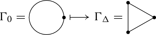
For a given graph $\Gamma$, we denote the set of isomorphism classes of graphs homeomorphic to $\Gamma$ by ${\mathcal {G}}(\Gamma )$. Then $\prec$ defines a partial order in ${\mathcal {G}}(\Gamma )$, which has a unique minimal element $\Gamma _0$ obtained by smoothing all bivalent vertices of $\Gamma$.

Besides, some of the graphs in ${\mathcal {G}}(\Gamma )$ can be realised as simplicial complexes. Let ${\mathcal {G}}_\Delta (\Gamma )$ be the subset of ${\mathcal {G}}(\Gamma )$ consisting of simplicial complexes. Then ${\mathcal {G}}_\Delta (\Gamma )$ has a unique minimal element $\Gamma _\Delta$ with respect to the partial order $\prec$ defined above, which can be obtained from $\Gamma _0$ by a series of subdivisions according to the following rules.

• 1. Subdivide each simple loop twice so that it forms a triangle.

  

• 2. Subdivide all multiple edges except for one of each.

  

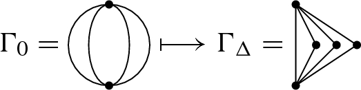
We call $\Gamma _\Delta$ the minimal simplicial representative of ${\mathcal {G}}(\Gamma )$.

A graph $\Gamma$ is called combinatorially k-connected if it has at least two vertices and for any pair $\{v,w\}$ of distinct vertices, there exist k internally-disjoint paths between v and w. A singleton graph consisting of one vertex without edges will be regarded as combinatorially 1-connected but not k-connected for any $k\ge 2$. Due to Menger’s theorem the combinatorial k-connectedness is equivalent to the fact that it is not possible to pick a set of $k-1$ distinct vertices, $K\subset V(\Gamma )$, that disconnects $\Gamma$. In other words, the induced subgraph spanned on vertices $V(\Gamma )\setminus K$ is never disconnected. See [22, Chapters 2 and 7] for detail.

We say that a graph $\Gamma$ is topologically k-connected if its minimal simplicial representative $\Gamma _\Delta$ is combinatorially k-connected. In this paper, topological connectivity is the default definition of connectivity, hence topologically k-connected graphs will be called just k-connected.

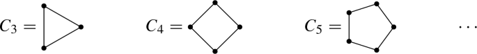
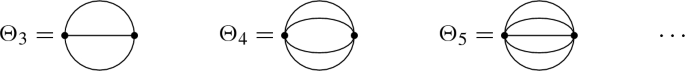
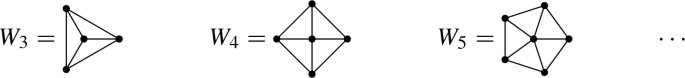
Example 1

The following holds. Let $k\ge 3$.

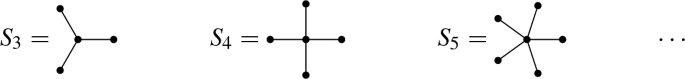
• Star graphs $S_k$ are 1-connected but not 2-connected.

  

• Cyclic graphs $C_k$ are 2-connected but not 3-connected.

  

• Graphs $\Theta _k$ are topologically 2-connected but not 3-connected.

  

• Wheel graphs $W_k$ are 3-connected.

  

• Any topologically non-2-connected graph has a vertex $v_0$ such that $\Gamma \setminus \{v_0\}$ is not connected.

Let $\Gamma$ be a graph. In further parts of this paper, we will often consider the space of all topological embeddings from $S_3$ to $\Gamma$.

This means that embedding $\iota$ may not the map the endpoint each leaf of $S_3$ to a vertex of $\Gamma$. However, it must send the central vertex of $S_3$ to an essential vertex of $\Gamma$. We say that two such embeddings $\iota$ and $\iota '$ are equivalent if they are isotopic as embeddings (up to automorphisms of $S_3$) between topological spaces. We denote the resulting quotient space by $\Gamma ^{S_3}$. As a result, $\Gamma ^{S_3}$ is a finite discrete set whose each element can be (uniquely) characterised by a pair $(v,{\mathbf {e}}=\{e_1,e_2,e_3\})$, where v is a vertex and $e_i$’s are three distinct edges adjacent to v.

Presentations of the braid group for particles in ${\mathbb {R}}^2$

In this paper we will often make references to different presentations of the planar braid group ${\mathbf {B}}_n({\mathbb {R}}^2)$. Let us next briefly review the relevant presentations. As a general reference for this subsection, we direct the reader to [23]. We start with the Artin presentation of ${\mathbf {B}}_n({\mathbb {R}}^2)$. In this presentation, generators of ${\mathbf {B}}_n({\mathbb {R}}^2)$ are called Artin generators. We assume that the initial configuration is such that particles $1,\ldots , n$ are aligned on a line segment in ${\mathbb {R}}^2$ in an equidistant way. The Artin generator $\sigma _i$ exchanges particle i with particle $i+1$ in a clockwise direction while other particles remain in their fixed positions (the choice of anti-clockwise exchange is a matter of convention). In this way, we obtain the set of $n-1$ generators $\sigma _1,\ldots ,\sigma _{n-1}$. Clearly, Artin generators involving disjoint sets of particles commute with each other, i.e. $\sigma _i\sigma _j=\sigma _j\sigma _i$ for $|i-j|\ge 2$. On the other hand, Artin generators involving triples of consecutive particles satisfy the braiding relation, i.e. $\sigma _i\sigma _{i+1}\sigma _i=\sigma _{i+1}\sigma _i\sigma _{i+1}$ for $i\in \{1,\ldots , n-2\}$.

When applied to a special class of unitary representations of ${\mathbf {B}}_n({\mathbb {R}}^2)$, the braiding relation leads to the celebrated Yang–Baxter equation. This concerns high-dimensional representations of ${\mathbf {B}}_n({\mathbb {R}}^2)$ to unitary operators acting on the Hilbert of n particles. We assume that the Hilbert space of a single particle is finite-dimensional, ${\mathcal {H}}_1={\mathbb {C}}^d$. Recall that the n-particle Hilbert space is the n-fold tensor product of single-particle spaces, i.e. ${\mathcal {H}}_n=\left( {\mathbb {C}}^d\right) ^{\otimes n}$. The Yang–Baxter equation is an equation for a unitary operator $R:\ {\mathbb {C}}^d\otimes {\mathbb {C}}^d\rightarrow {\mathbb {C}}^d\otimes {\mathbb {C}}^d$, called the R-matrix, that satisfies

$$\begin{aligned} (R\otimes \mathbb {1})(\mathbb {1}\otimes R)(R\otimes \mathbb {1})=(\mathbb {1}\otimes R)(R\otimes \mathbb {1})(\mathbb {1}\otimes R). \end{aligned}$$

(2)

The corresponding representation ${\mathbf {B}}_n({\mathbb {R}}^2)\rightarrow U(d^n)$ is constructed by assigning

$$\begin{aligned}\sigma _i\mapsto U_i:=\mathbb {1}\otimes \ldots \otimes \mathbb {1}\otimes R_{i,i+1}\otimes \mathbb {1}\otimes \ldots \otimes \mathbb {1}.\end{aligned}$$

Because the R-matrix satisfies Eq. (2), operators $U_i$ automatically satisfy the braiding relation. We will revisit this construction in Sect. 5.

Another presentation of ${\mathbf {B}}_n({\mathbb {R}}^2)$ that will be crucial for this paper uses only two generators. This is done by introducing the so-called total braid $\delta :=\sigma _1\sigma _2\ldots \sigma _{n-1}$. By utilising the commutative and braiding relations for Artin generators, one can verify that $\sigma _{i+1}=\delta \sigma _i\delta ^{-1}$. This allows one to recursively express any Artin generator as $\sigma _{i+1}=\delta ^{i}\sigma _1\delta ^{-i}$. When expressed in terms of generators $\delta$ and $\sigma _1$, braiding and commutative relations have the following forms

$$\begin{aligned}&\sigma _1\delta \sigma _1\delta ^{-1}\sigma _1=\delta \sigma _1\delta ^{-1}\sigma _1\delta \sigma _1\delta ^{-1}, \\&\quad \sigma _1\delta ^{j-i}\sigma _1\delta ^{i-j}=\delta ^{j-i}\sigma _1\delta ^{i-j}\sigma _1{\quad \mathrm {\ for\ }}|i-j|\ge 2. \end{aligned}$$

The completeness of the relations can be shown directly by a simple computation of substitutions. One may refer [24] or [23].

Presentations of Graph Braid Groups

Throughout this section, we assume that i) graph $\Gamma$ is finite, connected and has at least one essential vertex, ii) $\Gamma$ is sufficiently subdivided with respect to a fixed $n>1$. This means that the edge-length of every path between two essential vertices is at least $n-1$ and the edge-length of every loop is at least $n+1$.

Morse presentations

We first review Farley-Sabalka’s algorithm [10] which provides a group presentation of the graph braid group for any graph in terms of cells of an appropriate Morse complex. Certain features of Morse presentations of graph braid groups will be key ingredients of some of our proofs in later subsections. Farley-Sabalka’s algorithm realises a specific instance of Forman’s discrete Morse theory [25] on the discrete configuration space, $D_n(\Gamma )$. A discrete configuration space is a regular cube complex that is a deformation retract of $C_n(\Gamma )$. For the deformation-retracion $C_n(\Gamma )\rightarrow D_n(\Gamma )$ to work, $\Gamma$ has to be sufficiently subdivided with respect to the particle number n [26, 27]. Cells of $D_n(\Gamma )$ have the following form

$$\begin{aligned} c=\{c_1,c_2,\ldots ,c_n\}\subset \Gamma \mid {\overline{c}}_i\cap {\overline{c}}_j=\emptyset \quad \forall i\ne j \end{aligned}$$

where $\{c_i\}_{i=1}^n$ are mutually disjoint closed cells of $\Gamma$, i.e. they are either edges or vertices. Cell c can be viewed as a cube

Hence the dimension of c is given by $|E(\Gamma )\cap c|$. In this way, the discrete configuration space can also be viewed as a proper subset of $C_n(\Gamma )$.

The next step is the construction of a rooted spanning tree that determines the ordering of vertices of $\Gamma$. We choose a rooted spanning tree $(T,*)\subset \Gamma$ such that $*$ is univalent in T. Edges that belong to the complement of T in $\Gamma$ are called deleted edges. We assume that T is chosen so that the endpoints of deleted edges are always bivalent vertices.

We fix a planar embedding $T\subset {\mathbb {R}}^2$ and label vertices in T as follows.

• The root $*$ is labelled by 0.

• To determine labels of the remaining vertices, we imagine a thin ribbon neighbourhood of T. Starting from $*$ and travelling clockwise along the boundary of the ribbon, we label the visited vertices as $1,2,\ldots , |V|-1$.

We denote the deleted edge that is adjacent to $*$ by $e_0$ (if such an edge exists). Between any two vertices $\{v_1,v_2\}\subset V(\Gamma )$ there exists a unique edge path from $v_1,v_2$ in T. Such a path will be denoted by $[v_1,v_2]$. Therefore, by choosing a rooted spanning tree, we have a linear order on $V(\Gamma )$ that we denote by <. For any edge $e\in E(\Gamma )$ we define its initial and terminal vertices denoted by $\iota (e)$ and $\tau (e)$ respectively so that $\iota (e)>\tau (e)$. Similarly, for any $v\in V(\Gamma )$ we define e(v) as the edge for which $\iota (e(v))=v$. For an embedding between labelled graphs $f:\Gamma _1\rightarrow \Gamma _2$, we say that f is order-preserving if it preserves the order of vertices.

Example 2

For a subdivided $\Theta _k$, we may choose a rooted spanning tree $(T_k,*)$ as follows:

Then the ribbon of $T_k$ and labels are given below.

In the description of the graph braid group, we are particularly interested in loops and paths in $C_n(\Gamma )$. Note first that any path in $C_n(\Gamma )$ with its endpoints contained in $D_n(\Gamma )\subset C_n(\Gamma )$ is homotopy equivalent to a path that is entirely contained in $D_n(\Gamma )$. Furthermore, any path in $D_n(\Gamma )$ is homotopy equivalent to a path that is fully contained in the 1-skeleton of $D_n(\Gamma )$. In particular, any element ${\mathbf {B}}_n(\Gamma )$ can be represented as a word of 1-cells on $D_n(\Gamma )$. More precisely, cell $\{e,v_1,\ldots ,v_{n-1}\}$ is viewed as a directed path from $\{\iota (e),v_1,\ldots ,v_{n-1}\}$ to $\{\tau (e),v_1,\ldots ,v_{n-1}\}$.

The general idea of the discrete Morse theory is to contract configuration space $D_n(\Gamma )$ to a much smaller Morse complex $M_n(\Gamma )$ whose 1-skeleton is a wedge of circles based at the same point given by configuration $\{0,1,\ldots ,n-1\}$. Then, one uses the fact that ${\mathbf {B}}_n(\Gamma )\cong \pi _1\left( M_n(\Gamma )\right)$, i.e. ${\mathbf {B}}_n(\Gamma )$ is generated by the circles in the 1-skeleton of $M_n(\Gamma )$.

The construction of discrete Morse theory relies on the notion of Morse matching. A Morse matching is a collection of partially defined maps $\{W_d\}_{d=0}^{n}$ where $W_i$ maps some of d-cells in $D_n(\Gamma )$ to some of $(d+1)$-cells. In Farley-Sabalka’s algorithm the Morse matching can be understood in terms of imposing certain rules for particle movement on $\Gamma$. A d-dimensional cell $c\in D_n(\Gamma )$ is viewed as a move where d particles simultaneously slide along edges $e\in E(\Gamma )\cap c$ in the direction from $\iota (e)$ to $\tau (e)$. We say that an edge $e\in c$ is $order-respecting$ if $e\subset T$ and there are no vertices $v\in c$ for which $v<\tau (e)$ and $\tau (e(v))=\tau (e)$. Intuitively, on junctions in $\Gamma$ only particles that have no other particles to their right (in terms of vertex ordering on T) are allowed to move first. In a similar spirit one defines blocked vertices as vertices whose movement is blocked in c by some other particles. Vertex $v\in c$ is blocked if there exists $c_i\in c$ such that $\tau (e(v))\cap c_i\ne \emptyset$. Clearly, any edge $e\in c$ is either order-respecting or non order-respecting. Similarly, $v\in c$ can be either blocked or unblocked.

Definition 1

A cell $c\in D_n(\Gamma )$ is critical if and only all vertices $v\in V(\Gamma )\cap c$ are blocked and all edges $e\in E(\Gamma )\cap c$ are non order-respecting.

The definition of map $W_d$ is recursive. Namely, the domain of $W_d$ consists of cells that do not belong to the image of $W_{d-1}$ and are not critical. For such cells, $W_d$ finds the lowest unblocked vertex in c, $v_0$, and replaces it with edge e(v), i.e.

$$\begin{aligned}W_d(c)=\left( c\setminus \{v_0\}\right) \cup \{e(v_0)\}.\end{aligned}$$

Cells that belong to the domain of some $W_d$ are called redundant and cells that belong to the image of some $W_{d}$ are called collapsible. The Morse complex $M_n(\Gamma )$ is a complex whose d-skeleton consists of critical d-cells in $D_n(\Gamma )$. Importantly, any d-cell c in can be mapped to $M_n(\Gamma )$ as a word that consists only of critical cells. This is done by means of the principal reduction F. We will specify this construction only for 1-cells as this is the only relevant case for this paper. To this end, consider the boundary word of 2-cell $W_1(c)$ for a redundant cell c and bring it to the form cw where w is a word of appropriate 1-cells. Then, we define the principal reduction of a redundant c as $F(c)=w^{-1}$. The action of F is extended to critical sells as $F(c)=c$ and to collapsible cells as $F(c)=1$. We extend F to any word of 1-cells in a natural way. By applying map F to any word sufficiently many times, we always end up with a word that consists only of critical cells. Such a word is invariant under map F. Let us denote such a stable iteration of F by $F^\infty$. We are now ready to state the central theorem of this subsection.

Theorem 2

( Farley-Sabalka). Group ${\mathbf {B}}_n(\Gamma )$ is generated by critical 1-cells in $D_n(\Gamma )$. Relators are given by $F^\infty (w)$ where w goes through boundary words of all critical 2-cells in $D_n(\Gamma )$.

Recall that any critical 1-cell has the form $c=\{e,v_1,\ldots ,v_{n-1}\}$ where e is a non order-respecting edge and all $\{v_i\}_{i=1}^{n-1}$ are blocked. We will distinguish the following two types of critical 1-cells.

• 1. Critical cells associated with an essential vertex, i.e. $e\in T$.

• 2. Critical cells associated with a deleted edge, i.e. $e\in \Gamma \setminus T$.

A critical cell at an essential vertex has the following properties i) $\tau (e)$ is an essential vertex and there exists i such that $\tau (e(v_i))=\tau (e)$ and $\tau (e)<v_i<\iota (e)$, ii) for every i, we have $\tau (e(v_i))=v_j$ for some $i\ne j$ or $\tau (e(v_i))=\iota (e)$. Hence, the form of such a critical 1-cell can be uniquely determined by specifying i) the relevant essential vertex, ii) the distribution of particles on leaves incident at the essential vertex and iii) the leaf at v containing the non-order respecting edge in c. If the essential vertex is v and v is of valence k, such a critical cell will be denoted by $v_i({\mathbf {b}})$, where $i\in \{1,\ldots ,k-1\}$ is the leaf containing the non order-respecting edge and ${\mathbf {b}}=(b_1,b_2,\ldots ,b_{k-1})$ is a sequence of nonnegative integers that specifies the distribution of particles on leaves at vertex v.

Furthermore, the assumption that end-vertices of all deleted edges are bivalent implies that all critical cells that are associated with a deleted edge e are of the form $\{e,0,1,\ldots ,n-2\}$ if $\tau (e)\ne *$ and $\{e,1,2,\ldots ,n-1\}$ otherwise.

Note also that under the above assumptions about the choice of the spanning tree, there is just one critical 0-cell in $D_n(\Gamma )$, namely $\{0,1,\ldots ,n-1\}$. Hence, the 1-skeleton of $M_n(\Gamma )$ consists of 1-cells that are topological circles based at the unique 0-cell.

In the following subsections we establish a correspondence between geometric generators of ${\mathbf {B}}_n(\Gamma )$ and the above two types of critical 1-cells. Namely, critical cells at essential vertices will correspond to generators of the star type and critical cells associated with deleted edges will correspond to generators of the loop type.

Generators of the star type

One of the building blocks in geometric presentations of graph braid groups is an exhaustive description of ${\mathbf {B}}_n(\Gamma )$ when $\Gamma =S_k$, a star graph with k leaves. This is because for any graph $\Gamma$ generators of ${\mathbf {B}}_n(S_k)$ can be regarded as generators of ${\mathbf {B}}_n(\Gamma )$. To see this, for an essential vertex $v\in V(\Gamma )$ of valency k consider the following order-preserving embedding of $S_k$ into spanning tree $T\subset \Gamma$ centred at v

where the central vertex of $S_k$ is mapped to v, the 0-th edge of $S_k$ is mapped to a path from $*$ to v and the i-th edge of $S_k$ ($0<i<k$) is mapped to the corresponding (subdivided) edge adjacent to v. For such an embedding, critical 1-cells of $D_n(\Gamma )$ at v are in a one-to-one correspondence with critical 1-cells of $D_n(S_k)$. Hence, $\iota _v$ indices a well-defined map from ${\mathbf {B}}_n(S_k)$ to ${\mathbf {B}}_n(\Gamma )$.

In the remaining part of this subsection we will introduce geometric generators of the star type and by writing down all relations between them we will reproduce the following well-known result.

Theorem 3

[28]. The n-braid group ${\mathbf {B}}_n(S_k)$ of the star graph $S_k$ is a free group of rank

The strategy for this subsection is to find for each critical 1-cell $c\in D_n(S_k)$ its corresponding loop $\gamma \subset C_n(\Gamma )$ such that the associated word of 1-cells, $w_\gamma$, satisfies $F^\infty (w_\gamma )=c$. To this end, we introduce a shorthand notation for the configuration where $a_i$ points occupies ith leaf of $S_k$. We denote the leaves by $e_0,\ldots ,e_{k-1}$ and the respective particle configuration by $e_0^{a_0}e_1^{a_1}\cdots e_k^{a_k}$.

We also denote by $\beta ^i$ the path from configuration ${\mathbf {x}}e_0$ to configuration ${\mathbf {x}}e_i$ for some abstract configuration ${\mathbf {x}}$ where the top particle from leaf $e_0$ is moved to leaf $e_i$. Consequently, by $\beta ^{-i}$ we denote the inverse of $\beta ^i$.

Definition 2

(Y-exchange). For a sequence ${\mathbf {a}}=(a_1,\ldots , a_{i-1})$ with $1\le a_j<k$, we define $\beta ^{\mathbf {a}}$ as the concatenation

$$\begin{aligned} \beta ^{\mathbf {a}}= \beta ^{a_1}\cdots \beta ^{a_{i-1}}. \end{aligned}$$

For $1\le a,b <k$, we define a loop, called a Y-exchange on leaves a, b as

$$\begin{aligned} \sigma _i^{{\mathbf {a}},a,b}:=\beta ^{{\mathbf {a}}}Y^{ab}\beta ^{-{\mathbf {a}}}:e_0^n\rightarrow e_0^n\in {\mathbf {B}}_n(S_k), \end{aligned}$$

where

$$\begin{aligned} -{\mathbf {a}}= (-a_{i-1},-a_{i-2},\ldots , -a_1), \end{aligned}$$

and $Y^{ab}$ is the commutator of $\beta ^a$ and $\beta ^b$

$$\begin{aligned} Y^{ab} := \beta ^{a,b,-a,-b}=\beta ^a\beta ^b\beta ^{-a}\beta ^{-b}. \end{aligned}$$

In particular,

$$\begin{aligned} \sigma _1^{a,b}=Y^{ab}. \end{aligned}$$

Remark 1

We will also use the notation $\sigma _i^{\mathbf {a}}$ when ${\mathbf {a}}=(a_1,\ldots , a_{i+1})$ to denote $\sigma _i^{{\mathbf {a}}',a_i,a_{i+1}}$ for ${\mathbf {a}}'=(a_1,\ldots , a_{i-1})$.

Remark 2

The Y-exchange move has been considered in many literatures. For example, Kurlin and Safi-Samghabadi in [29] described the motion of two objects having non-zero (but finite) size on a metric graph, which seems more realistic but is essentially the same as our situation.

Example 3

Paths $\beta ^{1,3,1}$ and $Y^{4,2}$ for respective starting configurations $e_0^7$ and $e_0^4e_1^2e_3^1$ are depicted in Fig. 1.

Fig. 1

Paths $\beta ^{1,3,1}$ and $Y^{4,2}$

Roughly speaking, $\sigma _i^{{\mathbf {a}},a,b}$ interchanges ith and $(i+1)$st particles by using 0th, ath and bth edges after moving the first $(i-1)$ particles to leaves determined by sequence ${\mathbf {a}}$. Since $\left( Y^{ab}\right) ^{-1}=Y^{ba}$ and $Y^{aa}=1$, we have

$$\begin{aligned} \left( \sigma _i^{{\mathbf {a}},a,b}\right) ^{-1}&=\sigma _i^{{\mathbf {a}},b,a},&\sigma _i^{{\mathbf {a}},a,b}&=1. \end{aligned}$$

(3)

Remark 3

By counting the number of possible sequences ${\mathbf {a}}=(a_1,\ldots ,a_{i+1})$ for $i=1,\ldots ,n-1$, we get that the total number of Y-exchanges in ${\mathbf {B}}_n(S_k)$ is

$$\begin{aligned} \sum _{i=1}^{n-1}(k-1)^{i-1}\left( {\begin{array}{c}k-1\\ 2\end{array}}\right) . \end{aligned}$$

Factors $(k-1)^{i-1}$ come from choosing $i-1$ from $k-1$ leaves to accommodate the first $i-1$ particles. Factors $\left( {\begin{array}{c}k-1\\ 2\end{array}}\right)$ stem from the choice of two leaves where the exchange of particles i and $i+1$ takes place.

Next, we will proceed with the description of relations between the star-generators. To this end, we need to set up some more notation. Consider a path that connects configuration $e_0^n$ with configuration $e_0^{n-\sum b_j}e_1^{b_1}\cdots e_{k-1}^{b_{k-1}}$. Such a path will be unambiguously determined by the following sequence of nonnegative integers ${\mathbf {b}}=(b_1,\ldots , b_{k-1})$ that encodes the final particle configuration with $b_i$ particles on leaf $e_i$. Namely, we associate with ${\mathbf {b}}$ the following sequence

$$\begin{aligned} {{\overline{{\mathbf {b}}}}} = (\underbrace{k-1,k-1,\ldots , k-1}_{b_{k-1}},\underbrace{k-2,k-2,\ldots , k-2}_{b_{k-2}},\ldots ,\underbrace{1,1,\ldots , 1}_{b_1}). \end{aligned}$$

Path $\beta ^{{{\overline{{\mathbf {b}}}}}}$ connects configuration $e_0^n$ with configuration $e_0^{n-\sum b_j}e_1^{b_1}\cdots e_{k-1}^{b_{k-1}}$ as desired. Moreover, when written as a word of 1-cells of $D_n(\Gamma )$, $\beta ^{{{\overline{{\mathbf {b}}}}}}$ consists only of collapsible cells. To see this, note first that all 1-cells associated with one-particle moves in $\beta ^{{{\overline{{\mathbf {b}}}}}}$, $c=\{e,v_1,\ldots ,v_{n-1}\}$, are such that i) e is order-respecting and ii) vertex $\iota (e)$ is the lowest unblocked vertex in the 0-cell $c_0=\{\iota (e),v_1,\ldots ,v_{n-1}\}$. This in turn means that $c=W_0\left( c_0\right)$, i.e. c is collapsible. Using similar arguments, one can check that a critical cell $v_i({\mathbf {b}})$ for ${\mathbf {b}}=(b_1,\ldots ,b_{k-1})$ corresponds to the following concatenation of paths

$$\begin{aligned} v_i({\mathbf {b}}) = F^\infty \left( \beta ^{\overline{{\mathbf {b}}+e_i}}\cdot \beta ^{-i}\cdot \beta ^{-{{\overline{{\mathbf {b}}}}}}\right) , \end{aligned}$$

(4)

where

$$\begin{aligned} {\mathbf {b}}\pm e_i:=(b_1,\ldots , b_{i-1}, b_i\pm 1, b_{i+1},\ldots , b_{k-1}). \end{aligned}$$

To see this, note that the only critical cell in the word corresponding to 4 comes from the middle $\beta ^{-i}$-move and this is exactly critical cell $v_i({\mathbf {b}})$.

Proposition 1

The set $\{\sigma _i^{\mathbf {a}}\mid 1\le i\le n-1, {\mathbf {a}}=(a_1,\ldots , a_{i+1}), 1\le a_j\le k-1\}$ generates ${\mathbf {B}}_n(S_k)$.

Proof

Let us start with the simplest case of $n=2$. Any critical 1-cell has the form $\{e_i,w\}$ where $e_i$ is the edge from ith leaf that is incident to the central vertex v and w is a vertex that is adjacent to v and $v<w<\iota (e)$. According to our shorthand notation, such a 1-cell is denoted by $v_i(w)$. Any two-particle exchange has the form $\sigma _1^{a,b}=Y^{a,b}$. It is straightforward to see that

$$\begin{aligned}v_i(w)=F^\infty \left( Y^{\iota (e),w}\right) .\end{aligned}$$

In general, arbitrary critical cell $v_i({\mathbf {b}})\in D_n(\Gamma )$ can be expressed as a word of a number of star generators. In the remaining part of the proof, we will construct an inductive way for finding such a word. In order to handle arbitrary n, for any ${\mathbf {b}}=(b_1,\ldots ,b_{k-1})$ consider the following splitting ${\mathbf {b}}_1:=(0,\ldots , 0,b_i, b_{i+1},\ldots , b_{k-1})$, ${\mathbf {b}}_2:=(b_1,\ldots , b_{i-1},0,\ldots , 0)$. From equation (4) we get that $v_i({\mathbf {b}})$ is the following conjugation

$$\begin{aligned} v_i({\mathbf {b}})&\sim _{F^\infty } \beta ^{\overline{{\mathbf {b}}_1}} B \beta ^{-\overline{{\mathbf {b}}_1}},&B&=\beta ^i \beta ^{\overline{{\mathbf {b}}_2}} \beta ^{-i} \beta ^{-{{\overline{{\mathbf {b}}}}}_2}. \end{aligned}$$

Ley us next show that B is a word of Y-exchanges (modulo conjugation by appropriate paths) with the starting configuration being the end point of $\beta ^{{{\overline{{\mathbf {b}}}}}_1}$, i.e. $e_0^{n-b_i-\ldots -b_{k-1}}e_i^{b_i}\ldots e_{k-1}^{b_{k-1}}$. Indeed, for any sequence ${\mathbf {a}}=(a_1,\ldots ,a_\ell )$, we have the following:

$$\begin{aligned} \beta ^i\beta ^{{\mathbf {a}}}\beta ^{-i}\beta ^{-{\mathbf {a}}}=\beta ^i\beta ^{a_1}\beta ^{{\mathbf {a}}'}\beta ^{-i}\beta ^{-{\mathbf {a}}'}\beta ^{-a}=Y^{i,a_1}\cdot \beta ^{a_1}\left( \beta ^i\beta ^{{\mathbf {a}}'}\beta ^{-i}\beta ^{-{\mathbf {a}}'} \right) \beta ^{-a_1}, \end{aligned}$$

where ${\mathbf {a}}'=(a_2,\ldots , a_\ell )$. The above expression allows us to use the induction on the length of ${\mathbf {a}}$. Namely, by substituting ${\mathbf {a}}={{\overline{{\mathbf {b}}}}}_2$, we have

$$\begin{aligned} v_i({\mathbf {b}}) \sim _{F^\infty } \left( \beta ^{{{\overline{{\mathbf {b}}}}}_1}Y^{i,i-1}\beta ^{-{{\overline{{\mathbf {b}}}}}_1}\right) \cdot \left( \beta ^{{{\overline{{\mathbf {b}}}}}_1}\beta ^{i-1}\left( \beta ^i\beta ^{\overline{{\mathbf {b}}'}}\beta ^{-i}\beta ^{-\overline{{\mathbf {b}}'}}\right) \beta ^{-(i-1)}\beta ^{-{{\overline{{\mathbf {b}}}}}_1}\right) \\ =\sigma _{i_1}^{{{\overline{{\mathbf {b}}}}}_1,i,i-1}\cdot \left( \beta ^{{{\overline{{\mathbf {b}}}}}_1}\beta ^{i-1}\left( \beta ^i\beta ^{\overline{{\mathbf {b}}'}}\beta ^{-i}\beta ^{-\overline{{\mathbf {b}}'}}\right) \beta ^{-(i-1)}\beta ^{-{{\overline{{\mathbf {b}}}}}_1}\right) , \end{aligned}$$

where $\overline{{\mathbf {b}}'}=(b_1,\ldots ,b_{i-1}-1)$ and $i_1=1+b_{k-1}+b_{k-2}+\ldots +b_i$. By iterating the above inductive step for $\beta ^i\beta ^{\overline{{\mathbf {b}}'}}\beta ^{-i}\beta ^{-\overline{{\mathbf {b}}'}}$, we get that $v_i({\mathbf {b}})$ can be expressed as the $F^\infty$-image of a concatenation of the resulting star generators. $\square$

Proposition 2

There are relations among $\sigma _i^{\mathbf {a}}$’s as follows:

• 1. Pseudo-commutative relation: for $|j-i|\ge 2$,

  $$\begin{aligned} \sigma _j^{a_1\ldots a_{j+1}}\sigma _i^{a_1\ldots a_{i+1}} = \sigma _i^{a_1\ldots a_{i+1}}\sigma _j^{a_1\ldots a_{i-1}a_{i+1}a_ia_{i+2}\ldots a_{j+1}}. \end{aligned}$$

  (5)

• 2. Pseudo-braid relation: for $1\le i\le n-2$,

  $$\begin{aligned}&\sigma _{i+1}^{a_1\ldots a_{i-1}a_i a_{i+1}a_{i+2}}\sigma _i^{a_1\ldots a_{i-1}a_i a_{i+2}}\sigma _{i+1}^{a_1\ldots a_{i-1}a_{i+2}a_i a_{i+1}}\nonumber \\&\quad =\sigma _i^{a_1\ldots a_{i-1}a_i a_{i+1}}\sigma _{i+1}^{a_1\ldots a_{i-1}a_{i+1}a_i a_{i+2}}\sigma _i^{a_1\ldots a_{i-1}a_{i+1}a_{i+2}}. \end{aligned}$$

  (6)

Proof

The relations can be checked in a straightforward way by using the definition of star generators and expanding each generator as

$$\begin{aligned}\sigma _i^\mathbf{b}=\beta ^{b_1}\ldots \beta ^{b_{i-1}}Y^{b_i,b_{i+1}}\beta ^{-b_{i-1}}\ldots \beta ^{-b_1},\end{aligned}$$

where $Y^{b_i,b_{i+1}}=\beta ^{b_i}\beta ^{b_{i+1}}\beta ^{-b_i}\beta ^{-b_{i+1}}$ and cancelling $\beta ^x\beta ^{-x}$ whenever such an expression is encountered. $\square$

Note that relation (5) becomes trivial if $a_i=a_{i+1}$ or $a_j=a_{j+1}$. Similarly, relations (6) become trivial is at least one of the following equations is satisfied: $a_i=a_{i+1}$, $a_{i+1}=a_{i+2}$, $a_i=a_{i+2}$. In particular, relations (6) are nontrivial if and only if $k\ge 4$.

Let $G_{n,k}$ be the abstract group whose generators are all $\sigma _i^{{\mathbf {a}}}$ and relations are given by (5) and (6).

Lemma 1

Group $G_{n,k}$ is a free group of rank $N_1(n,k)$ that is generated by $\sigma _i^{{\mathbf {a}}}$ such that $1\le a_1\le a_2\le \ldots \le a_{i-1}\le a_{i+1}$ and $a_{i}<a_{i+1}$.

Proof

We consider the group presentation of $G_{n,k}$ having all $\sigma _j^{\mathbf {a}}$ as generators and relations as in (5) and (6).

First, let us consider generators $\sigma _{j}^{{\mathbf {a}}}$ with $j=n-1$. Whenever $a_{i+1}<a_i$ for some $i\le n-3$, we can use a preudo-commutative relation (5) to swap $a_{i+1}$ and $a_i$. That is, we apply the following Tietze transformation

$$\begin{aligned}\sigma _{n-1}^{a_1\ldots a_{n}}=\sigma _i^{a_1\ldots a_{i+1}}\sigma _{n-1}^{a_1\ldots a_{i-1}a_{i+1}a_ia_{i+2}\ldots a_{n}}\left( \sigma _i^{a_1\ldots a_{i+1}}\right) ^{-1}\end{aligned}$$

to obtain a presentation of $G_{n,k}$ where every $\sigma _{n-1}^{{\mathbf {a}}}$ satisfies $a_i\le a_{i+1}$. Applying analogous Tietze transformations for every $i\in \{1,\ldots ,n-3\}$, we get a presentation of $G_{n,k}$ where sequences ${\mathbf {a}}$ satisfy

$$\begin{aligned}a_1\le a_2\le \ldots \le a_{n-2}.\end{aligned}$$

Let us next show how pseudo-braiding relations (6) allow us to arrange triples $a_{n-2}, a_{n-1}, a_n$. Whenever the triple $a_{n-2}, a_{n-1}, a_n$ consists of pairwise distinct integers, relation (6) involves the following three generators

$$\begin{aligned} \sigma _{n-1}^{a_1\ldots a_{n-3} a_{n-2} a_{n-1} a_n},\ \sigma _{n-1}^{a_1\ldots a_{n-3} a_{n-1} a_n a_{n-2}}\quad \text { and }\quad \sigma _{n-1}^{a_1\ldots a_{n-3} a_{n-1} a_n a_{n-2}} \end{aligned}$$

and two more generators with $j=n-2$. Note that the above three generators contain all permutations of $a_{n-2}, a_{n-1}, a_n$. Therefore, no matter what magnitudes of these numbers are, one can always find an appropriate Tietze transformation that yields a presentation of $G_{n,k}$ with

$$\begin{aligned} a_{n-2}&\le a_n,&a_{n-1}&<a_n. \end{aligned}$$

Summing up, using relations (5) and (6) we are able to obtain a presentation of $G_{n,k}$ whose generators $\sigma _{n-1}^{{\mathbf {a}}}$ are associated with sequences ${\mathbf {a}}$ such that $1\le a_1\le a_2\le \ldots \le a_{n-2}\le a_n$ and $a_{n-1}<a_n$. Let $a_n=j$. Then the number of such sequences is $\left( {\begin{array}{c}n+j-3\\ j-1\end{array}}\right) (j-1)$, where the factor $(j-1)$ comes from the choice of $1\le a_{n-1}<j=a_n$. Therefore the total number of generators $\sigma _{n-1}^{\mathbf {a}}$ is exactly

$$\begin{aligned} \sum _{j=1}^{k-1}\left( {\begin{array}{c}n+j-3\\ j-1\end{array}}\right) (j-1). \end{aligned}$$

It is straightforward to check that this number is the same as $N_1(n,k)-N_1(n-1,k)$.

Finally, by applying analogous Tietze transformations for $\sigma _{n-2}^{\mathbf {a}}, \sigma _{n-3}^{\mathbf {a}}$ and so on, we can reduce all relations and end up with exactly $N_1(n,k)$ generators. $\square$

Theorem 4

The abstract group $G_{n,k}$ is isomorphic to the braid group ${\mathbf {B}}_n(S_k)$ via the canonical map $\phi :G_{n,k}\rightarrow {\mathbf {B}}_n(S_k)$ which sends $\sigma _i^{\mathbf {a}}$ to an n-braid in $S_k$ represented by $\sigma _i^{\mathbf {a}}$.

Proof

By Propositions 1 and 2, map $\phi$ is a surjective group homomorphism. Since both $G_{n,k}$ and ${\mathbf {B}}_n(S_k)$ are free groups of the same rank $N_1$, the surjective homomorphism $\phi$ becomes an isomorphism since any finitely generated free groups are Hopfian. $\square$

The construction of star generators in terms of Y-exchanges can also be generalised so that it applies to any graph $\Gamma$. This is done by considering an appropriate embedding of $S_k$ into $\Gamma$ as explained in the definition below.

Definition 3

For each essential vertex $v\in V(\Gamma )$ of valency $k\ge 3$ and a sequence ${\mathbf {a}}=(a_1,\ldots , a_{i+1})$ with $1\le a_j\le k-1$, we define $\sigma _i^{v;{\mathbf {a}}}$ by the image of $\sigma _i^{{\mathbf {a}}}\in {\mathbf {B}}_n(S_k)$ under the map $(\iota _v)_*$

$$\begin{aligned} \sigma _i^{v;{\mathbf {a}}} = (\iota _v)_*(\sigma _i^{{\mathbf {a}}}), \end{aligned}$$

where $\iota _v$ is the order-preserving embedding

$$\begin{aligned} \iota _v:(S_k,*)\rightarrow (T,*)\subset (\Gamma ,*) \end{aligned}$$

such that $\iota _v$ maps the central vertex of $S_k$ to the chosen vertex v. We also denote $\sigma _1^{v;a,b}$ by $Y^{v;ab}$.

Generators of loop type

Generators of the loop type are in a one-to-one correspondence with deleted edges $e\in \Gamma \setminus T$. To each deleted edge e we assign a unique loop in $\Gamma$ using the path in T that joins $\iota (e)$ and $\tau (e)$. The form of such a loop is $e\cup [\iota (e),\tau (e)]$ and we give it an orientation that agrees with the canonical orientation of e – from $\iota (e)$ to $\tau (e)$. We also distinguish one deleted edge $e_0$ being the deleted edge which is adjacent to the root of T. Edge $e_0$ will define a move which will be the counterpart of the total braid $\delta$ in ${\mathbf {B}}_n({\mathbb {R}}^2)$. Other edges will correspond to one-particle moves. The base point for all moves is such that all particles are resting on the edge in T which is incident to the root $*$. In terms of the corresponding Morse complex $M_n(\Gamma )$, all loops are based at the point corresponding to the unique critical 0-cell $\{0,1,\ldots ,n-1\}$. The loop generators are constructed as follows (see Fig. 2 an illustration of these generators).

• 1. If $e=e_0$, its corresponding loop is the following embedding of circle graph $C_k$.

  

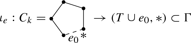
  Generator $\delta$ is the image of the generator of ${\mathbf {B}}_n(S^1)$ which takes the top particle around $C_k$ and moves it to the bottom of the line. Generator $\delta$ will be called the circular move. Such a move is unique (up to homotopy) provided that edge $e_0$ exists.

• 2. If $e\ne e_0$, then there is an embedding $\iota _e:Q\rightarrow \Gamma$, where Q is the lollipop graph

  

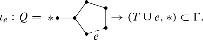
  In this case, generator $\gamma$ is the image of a particular generator of ${\mathbf {B}}_n(Q)$ which moves the top particle around $\gamma$ while the remaining $(n-1)$ particles stay fixed on their positions on the edge which is the stick of the lollipop. We call $\gamma$ a one-particle move. Then there are exactly $(b_1(\Gamma )-1)$ such generators where $b_1(\Gamma )$ is the first Betti number of $\Gamma$.

Fig. 2

Generators of loop type

Let us next define another one-particle move $\gamma _0$ for ${\mathbf {B}}_n(\Gamma )$ associated with edge $e_0$. Since $\Gamma$ is connected and contains at least one essential vertex, the loop represented by $e_0$ must contain an essential vertex v. This means that we have a subgraph homeomorphic to the lollipop graph Q whose loop is represented by $e_0$ and the lollipop’s stick is some edge incident at v that is not contained in the loop. We denote by $e_{0}^v$ and $e_{1}^v$ the two edges that are incident at v and lie on the loop in Q. Edge $e_{0}^v$ is defined as the one which is closer to $*$ than $e_{1}^v$ in T. We denote the other edge incident at v by $e_{2}^v$.

We define a braid $\gamma _0$ which is a one-particle move defined as follows. We first move the top $n-1$ particles to the edge $e_{2}^v$ and then we move the remaining nth particle along the loop represented by $e_0$. After the nth particle finishes the loop and returns to its original position, we move back the other $n-1$ particles from $e_{2}^v$ to their initial positions.

Then $\gamma _0$ can be expressed as a word involving $\sigma ^{v;{\mathbf {a}}}$, $\gamma _0$ and $\delta$. More specifically, Y-exchanges $\sigma _i^{v;{\mathbf {a}}}$ at v satisfy the following relation

$$\begin{aligned} \gamma _0=\sigma _{n-1}^{v;2,\ldots ,2,1}\sigma _{n-2}^{v;2,\ldots ,2,1}\cdots \sigma _1^{v;2,1}\delta . \end{aligned}$$

(7)

Moreover, for any ${\mathbf {a}}=(a_1,\ldots ,a_{i+1})$ such that $a_i\in \{1,2\}$ for all i, we have another relation

$$\begin{aligned} \sigma _{i+1}^{v;{\mathbf {a}}'}&=\delta \cdot \sigma _i^{v;{\mathbf {a}}}\cdot \delta ^{-1},&{\mathbf {a}}'&=(1,a_1,\ldots ,a_{i+1}). \end{aligned}$$

(8)

Both of the above relations can be verified by visualising their corresponding moves. LHS and RHS of the above equations are essentially the same moves up to some backtracking.

Remark 4

Let us next briefly argue how the above relations (7) and (8) will be used to relate graph braid groups to ${\mathbf {B}}_n({\mathbb {R}}^2)$. Namely, consider quotient group ${\mathbf {B}}_n(Q)/\langle \gamma _0\rangle$ which is generated only by star generators $\sigma _i^{v;{\mathbf {a}}}$. By (7), circular move is then expressed as

$$\begin{aligned}\delta =\sigma _1^{v;1,2}\sigma _2^{v;2,1,2}\ldots \sigma _{n-1}^{v;2,\ldots ,1,2}.\end{aligned}$$

Substituting the above expression in equation (8), we get

$$\begin{aligned} \sigma _1^{v;1,2}\sigma _2^{v;2,1,2}X\sigma _1^{v;1,2}X^{-1}&= \sigma _2^{v;1,1,2}\sigma _1^{v;1,2}\sigma _2^{v;2,1,2}, \end{aligned}$$

(9)

where

$$\begin{aligned} X&=\sigma _3^{v;2,2,1,2}\sigma _4^{v;2,\ldots ,2,1,2}\cdots \sigma _{n-1}^{v;2,\ldots ,2,1,2}. \end{aligned}$$

If we forget all decorations such as v and ${\mathbf {a}}$, then we can use pseudo-braiding relations for $S_3$ to show that X commutes with $\sigma _1^{v;1,2}$. Then, equation (9) simplifies to the ordinary braid relation.

Generation of graph braid groups and connectivity

The following theorem summarises the material contained in previous sections.

Theorem 5

The graph braid group ${\mathbf {B}}_n(\Gamma )$ for arbitrary $\Gamma$ is generated by the following moves

• 1. Y-exchanges

  $$\begin{aligned} \{\sigma _i^{v;{\mathbf {a}}}\mid 1\le i<n, v\in V, {\mathbf {a}}=(a_1,\ldots , a_{i+1}), 1\le a_j<{{\,\mathrm{val}\,}}(v)\}, \end{aligned}$$

• 2. $b_1(\Gamma )$-many one-particle moves

  $$\begin{aligned} \{\gamma _0,\ldots , \gamma _{b-1}\mid b=b_1(\Gamma )\}, \end{aligned}$$

• 3. one circular move $\delta$,

where $b_1(\Gamma )$ is the first Betti number of $\Gamma$.

Proof

This is a direct consequence of Farley-Sabalka’s algorithm and Proposition 1. Namely, any critical 1-cell associated with an essential vertex $v\in \Gamma$ is $F^\infty$-equivalent to a word of Y-exchanges $\sigma _i^{v;{\mathbf {a}}}$. Furthermore, any critical 1-cell associated with a deleted edge $e\ne e_0$ is $F^\infty$-equivalent to a word of 1-cells corresponding to the loop generator associated with e. This is because such a word contains only collapsible cells and one critical cell which is precisely $\{e,0,1,\ldots ,n-2\}$. By similar arguments, critical cell $\{e_0,1,2,\ldots ,n-1\}$ is $F^\infty$-equivalent to the word of 1-cells associated with circular move $\delta$. Hence, for every critical 1-cell in $D_n(\Gamma )$, we have found its corresponding geometric generator. By theorem 2, such geometric moves generate ${\mathbf {B}}_n(\Gamma )$. $\square$

Our next result states that for 2-connected graphs the number of Y-exchanges needed to generate ${\mathbf {B}}_n(\Gamma )$ can be greatly reduced.

Proposition 3

Let $\Gamma$ be a 2-connected graph. Then the braid group ${\mathbf {B}}_n(\Gamma )$ is generated by

$$\begin{aligned} \{Y^{v;ab}\mid v\in V, 1\le a<b<{{\,\mathrm{val}\,}}(v)\}\sqcup \{\gamma _0,\ldots ,\gamma _{b-1}\mid b=b_1(\Gamma )\}\sqcup \{\delta \}. \end{aligned}$$

Proof

It suffices to show that each $\sigma _i^{v;{\mathbf {a}}}$ can be expressed as a word of $Y^{w;ab}$, $\gamma _j$, and $\delta$. We use the induction on both i and the edge-length of the path $[*,v]$ in T. For $i=1$, there is nothing to prove for any v.

Suppose that v is the very first essential vertex when counting from $*$, i.e. there are no essential vertices in the interior of $[*,v]$. Let $v'$ be the essential vertex which is the end of $a_1$th edge incident at v. Since $\Gamma$ is 2-connected, $\Gamma _v=\Gamma \setminus {{\,\mathrm{Star}\,}}(v)$ is connected. Therefore there exists a path $\gamma \subset \Gamma _v$ from $v'$ to $*$. Such a path $\gamma$ defines a loop ${{\overline{\gamma }}}$ based at $*$ which is the union .

We use loop ${{\overline{\gamma }}}$ to define a braid of the circular type which sends the top particle around ${{\overline{\gamma }}}$ to the last position, just as the circular move $\delta$. We denote such a move by ${{\overline{\gamma }}}$ as well. Move ${{\overline{\gamma }}}$ is a word of $\gamma _j^{\pm 1}$ and $\delta$ so that

$$\begin{aligned} {{\overline{\gamma }}}=\gamma _{j_1}^{s_1}\ldots \gamma _{j_\ell }^{s_\ell }\delta , \end{aligned}$$

where $(j_1,\ldots ,j_\ell )$ is a sequence of indices of deleted edges that $\gamma$ passes and $s_k\in \{-1,1\}$, $1\le k\le \ell$, are exponents coming from orientations of the deleted edges relative to the orientation of $\gamma$. We also have a relation which is analogous to relation (8).

$$\begin{aligned} \sigma _i^{v;{\mathbf {a}}}&= {{\overline{\gamma }}}\sigma _{i-1}^{v;{\mathbf {a}}'}\left( {{\overline{\gamma }}}\right) ^{-1},&{\mathbf {a}}'&=(a_2,\ldots , a_{i+1}) \end{aligned}$$

By repeating the above inductive step for $\sigma _{i-1}^{v;{\mathbf {a}}'}$ and another loop associated with edge $e_{a_2}^v$ and so on, we end up with an expression that involves only one-particle moves, the circular move $\delta$ and $\sigma _1^{v;a_{i},a_{i+1}}$.

Now suppose that v is a vertex farther than the nearest vertices from $*$ and $i\ge 2$. As before, the connectivity of $\Gamma _v$ implies the existence of a path $\gamma \subset \Gamma _v$ from the $v'$ to $*$, where $v'\ne v$ is the vertex which is the end point of the $a_1$th edge adjacent to v.

Suppose that $\gamma$ does not intersect the path $[*,v]$ in T. Then the union defines a loop ${{\overline{\gamma }}}$ based at $*$ and by the exactly same argument as above, we have

$$\begin{aligned} \sigma _i^{v;{\mathbf {a}}} = {{\overline{\gamma }}}\sigma _{i-1}^{v;{\mathbf {a}}'}\left( {{\overline{\gamma }}}\right) ^{-1}, \end{aligned}$$

(10)

where

$$\begin{aligned} {\mathbf {a}}'&=(a_2,\ldots , a_{i+1}),&{{\overline{\gamma }}}&=\gamma _{j_1}^{s_1}\ldots \gamma _{j_\ell }^{s_\ell }\delta , \end{aligned}$$

and by the induction hypothesis, we are done.

Finally, suppose that $\gamma$ intersects the path $[*,v']$ at $w\ne *$. By taking the subpath of $\gamma$, we may assume that $\gamma$ is a composition of $\gamma '$ and $[w,*]$ such that $\gamma '$ is a path joining v and w and does not intersect $[*,v]$.

As before, it gives us loop ${{\overline{\gamma }}}=[*,v']\cup \gamma '\cup [w,*]$ based at $*$. In this case, ${{\overline{\gamma }}}$ can be regarded as a one-particle move and expressed as a word

$$\begin{aligned} {{\overline{\gamma }}}=\gamma _{j_1}^{s_1}\ldots \gamma _{j_\ell }^{s_\ell }, \end{aligned}$$

where $(j_1,\ldots ,j_\ell )$ is the sequence of indices of deleted edges defined as the same as before and $s_k\in \{-1,1\}$, $1\le k\le \ell$ are the exponents.

Let us denote two edges adjacent to w contained in $[*,v]$ and $\gamma '$ by $e_a^w$ and $e_b^w$, respectively. The conjugation ${{\overline{\gamma }}}^{-1}\sigma _i^{v;{\mathbf {a}}}{{\overline{\gamma }}}$ gives us a braid, which is a concatenation as follows:

• 1. Move the first particle along $[*,w]$ to the edge $e_b^w$.

• 2. Move the next $(i-2)$ particles onto edges adjacent to v by using the sequence $(a_2,\ldots , a_{i-1})$.

• 3. Interchange the positions of the next two particles by using the $a_i$th and $a_{i+1}$th edges adjacent to v and take them back to the edge at $*$.

• 4. Move the $(i-2)$ particles on edges of v back to the original position.

• 5. Move the first particle back to the original position.

Then indeed, this is a conjugate of $\sigma _{i-1}^{v;{\mathbf {a}}'}$ with ${\mathbf {a}}'=(a_2,\ldots , a_{i+1})$ by the braid $\sigma$ which interchanges positions of the first particle with the next i particles at w by using edges $e_a^w$ and $e_b^w$, which is a word of Y-exchanges

$$\begin{aligned} \sigma =\sigma _1^{w;b,a}\sigma _2^{w;a,b,a}\ldots \sigma _{i}^{w;a,\ldots ,a,b,a}. \end{aligned}$$

Therefore we have

$$\begin{aligned} \sigma _i^{v;{\mathbf {a}}} = {{\overline{\gamma }}}\cdot \sigma \cdot \sigma _{i-1}^{v;{\mathbf {a}}'}\cdot \sigma ^{-1}\cdot {{\overline{\gamma }}}^{-1} \end{aligned}$$

(11)

By induction hypothesis, not only $\sigma _{i-1}^{v;{\mathbf {a}}'}$ but also all $\sigma _j^{w;-}$ can be expressed as words of $\sigma _i^{w;-}$’s since w is closer to $*$ than v, which completes the proof. $\square$

Planar Triconnected Graphs

For the rest of the paper, we assume that $\Gamma$ is planar and we fix its planar embedding $\iota :\Gamma \rightarrow {\mathbb {R}}^2$. We denote the closures of connected components of the complement ${\mathbb {R}}^2\setminus \Gamma$ by $D_0,\ldots ,D_b$, where b is the first betti number of $\Gamma$. In particular, we assume that $D_b$ is the unbounded component.

Remark 5

If $\Gamma$ is 2-connected, then each bounded $D_i$ is homeomorphic to a closed disk and will be called a face of $\Gamma$.

We choose a bounded face, say $D_0$, whose boundary $\partial D_0$ shares at least one edge e with the unbounded face $\partial D_b$. By subdividing e if necessary, we may assume that there exists a bivalent vertex $*$ in the common boundary of $D_0$ and $D_b$

$$\begin{aligned} *&\in \partial D_0\cap \partial D_b,&{{\,\mathrm{val}\,}}(*)&=2. \end{aligned}$$

We denote the facial cycle $\partial D_0$ by $\delta$.

Let $(T,*)$ be a rooted spanning tree for $\Gamma$ such that every deleted edge has bivalent endpoints. Without loss of generality, we may assume that $\delta \setminus e_0\subset T$, or equivalently, $e_0\subset \Gamma \setminus T$ is a deleted edge representing the loop $\delta$.

Proposition 4

Let $\Gamma$ be a planar 2-connected graph with the first betti number b. Then ${\mathbf {B}}_n(\Gamma )$ admits a group presentation generated by Y-exchanges, one-particle moves and the circular move such that we obtain the classical braid group ${\mathbf {B}}_n({\mathbb {R}}^2)$ from ${\mathbf {B}}_n(\Gamma )$ by

• 1. taking the quotient by all one-particle moves $\{\gamma _0,\ldots ,\gamma _{b-1}\}$, and

• 2. identifying all Y-exchanges.

Proof

Let $(T,*)$ be a rooted spanning tree as above. Then ${\mathbf {B}}_n(\Gamma )$ admits a group presentation whose generators are Y-exchanges, one-particle moves and a circular move by Proposition 3.

It is clear that the induced map $\iota _*:{\mathbf {B}}_n(\Gamma )\rightarrow {\mathbf {B}}_n({\mathbb {R}}^2)$ kills all one-particle moves and identifies all $Y^{v;a,b}$’s. Therefore $\iota _*$ factors through ${\mathbf {B}}_n(\Gamma )/\sim$

where

$$\begin{aligned} {\mathbf {B}}_n(\Gamma )/\sim ={\mathbf {B}}_n(\Gamma )\bigg /\left\langle \gamma _0,\ldots ,\gamma _{b-1}, Y^{v;a,b}Y^{v';b',a'} \right\rangle \end{aligned}$$

for $1\le a<b<{{\,\mathrm{val}\,}}(v), 1\le a'<b'<{{\,\mathrm{val}\,}}(v')$ and $v, v'\in V$. Taking the quotient $\sim$ is the same as forgetting decorations ${\mathbf {a}}$ and v in $\sigma _i^{v;{\mathbf {a}}}$. Here we only sketch the proof of this fact, as it relies on the same inductive reasoning as the one that was used in the proof of Proposition 3. Namely, for an essential vertex v consider the inductive step where one assumes that $\sigma _j^{w;{\mathbf {a}}}\sim \sigma _j^{w';{\mathbf {b}}}$ for all $j<i$ and $w,w'<v$ and any sequences ${\mathbf {a}},\ {\mathbf {b}}$. Recursive relations (10) and (11) together with braiding and commutative relations for each $w,w'<v$ imply that $\sigma _i^{v;{\mathbf {a}}}\sim \sigma _i^{w;{\mathbf {b}}}$ for all $w<v$ and and appropriate ${\mathbf {b}}$. The base case is $\sigma _1^{v_0;1,2}$ where $v_0$ is the closest essential vertex to the root $*$.

Hence, pseudo-commutative star relations (5) become just the commutative relations in ${\mathbf {B}}_n(\Gamma )/\sim$ and lollipop relations (9) become the regular braiding relations. Therefore, we have

$$\begin{aligned} {{\overline{\sigma }}}_i{{\overline{\sigma }}}_j{{\overline{\sigma }}}_i^{-1}{{\overline{\sigma }}}_j^{-1}={\left\{ \begin{array}{ll} e &{} |i-j|>1;\\ {{\overline{\sigma }}}_j^{-1}{{\overline{\sigma }}}_i&{} |i-j|=1, \end{array}\right. } \end{aligned}$$

where for any v and $1\le a<b<{{\,\mathrm{val}\,}}(v)$.

In other words, there exists a surjective homomorphism $f:{\mathbf {B}}_n({\mathbb {R}}^2)\rightarrow {\mathbf {B}}_n(\Gamma )/\sim$ sending $\sigma _i$ to ${{\overline{\sigma }}}_i$. Since ${{\overline{\iota }}}_*\circ f$ is the identity on ${\mathbf {B}}_n({\mathbb {R}}^2)$, the map f is injective as well. Therefore f is in fact an isomorphism. $\square$

Example 4

Consider graph $\Theta _3$ from Fig. 3a. Denote by $\gamma$ the one-particle move where the first particle travels around the cycle which is disjoint from $*$ in the direction from v to w along [v, w] (it is the upper cycle on Fig. 3a). Moreover, denote by $\gamma '$ a move which involves particles 1 and 2 where i) particle 1 travels to branch $e_2^w$ through the solid edge [v, w], ii) particle 2 goes around the upper cycle (first along [v, w] in the direction from v to w and then back to v through the upper deleted edge) and iii) the first particle goes back through the solid edge [v, w]. Up to some backtracking moves, we have the following relations.

$$\begin{aligned} Y^{w;2,1}\gamma =\gamma ' Y^{v; 2,1}, \end{aligned}$$

(12)

$$\begin{aligned} \delta \gamma =\gamma ' \delta . \end{aligned}$$

(13)

Note, that after substituting expression for $\gamma '$ from (12) into (13) we obtain

$$\begin{aligned} \delta \gamma \delta ^{-1}=Y^{w;2,1}\gamma Y^{v;1,2}. \end{aligned}$$

(14)

After taking the quotient by one-particle move $\gamma$, Eq. (14) yields identification $Y^{w;1,2}\sim Y^{v; 1,2}$. Hence, by proposition 4, the quotient of ${\mathbf {B}}_n(\Theta _3)$ by one-particle cycles is isomorphic to ${\mathbf {B}}_n({\mathbb {R}}^2)$.

Example 5

Let $\vartheta _3$ be the graph which is the union of the theta graph $\Theta _3$ and an edge as depicted in Fig. 3b. We denote by $\gamma$ and $\gamma '$ the one-particle moves corresponding to the loops which are boundary of the right and left regions, respectively. Then as before, up to some backtracking moves, we have the following relation.

$$\begin{aligned} Y^{w;1,2}=\gamma ' Y^{v;1,2} \gamma Y^{z;2,1} \gamma '^{-1} Y^{z;1,2} \gamma . \end{aligned}$$

(15)

After taking the quotient by $\gamma , \gamma '$, this yields identification $Y^{w;1,2}\sim Y^{v;1,2}$.

Fig. 3

Settings for canonical moves on $\Theta _3$ and $\vartheta _3$

Definition 4

Let p, q be two essential vertices of valency $k, \ell$. For $1\le a<b<k$ and $1\le c<d<\ell$, two triples (p; a, b) and (q; c, d) are said to be $\Theta$-related if there exists and embedding $\iota$

$$\begin{aligned} \iota :(\Theta _3, T_{\Theta _3},*)\rightarrow (\Gamma , T,*)\quad \text { or }\quad \iota :(\vartheta _3, T_{\vartheta _3},*)\rightarrow (\Gamma , T,*) \end{aligned}$$

such that

$$\begin{aligned} \iota (v)&= p,&\iota (e_1^v)&= e_a^p,&\iota (e_2^v)&= e_b^p,\\ \iota (w)&= q,&\iota (e_1^w)&= e_c^q,&\iota (e_2^w)&= e_d^q. \end{aligned}$$

We define the equivalence relation generated by $\Theta$-relatedness and denote it by

$$\begin{aligned} (p;a,b)\sim _\Theta (q;c,d). \end{aligned}$$

Suppose that (p; a, b) and (q; c, d) are $\Theta$-related. Then two Y-exchanges $Y^{p;ab}$ and $Y^{q;cd}$ are the images of Y-exchanges $Y^{v;1,2}$ and $Y^{w;1,2}$ under the induced map

$$\begin{aligned} \iota _*:{\mathbf {B}}_n(\Theta _3)\rightarrow {\mathbf {B}}_n(\Gamma )\quad \text { or }\quad \iota _*:{\mathbf {B}}_n(\vartheta _3)\rightarrow {\mathbf {B}}_n(\Gamma ). \end{aligned}$$

Moreover, the induced map $\iota _*$ sends one-particle moves in ${\mathbf {B}}_n(\Theta _3)$ or ${\mathbf {B}}_n(\vartheta _3)$ to words of one-particle moves in ${\mathbf {B}}_n(\Gamma )$. It also maps a circular move in ${\mathbf {B}}_n(\Theta _3)$ to a word of one-particle moves and a circular move in ${\mathbf {B}}_n(\Gamma )$ as seen in the proof of Proposition 3.

Lemma 2

If (p; a, b) and (q; c, d) are $\Theta$-related, then Y-exchanges $Y^{p;ab}$ and $Y^{q;cd}$ are identified by taking the quotient by one-particle moves.

Proof

Let $\iota$ be an embedding of $\Theta _3$ or $\vartheta _3$ which makes (p; a, b) and (q; c, d) $\Theta$-related. As seen in Examples 4 and 5, two Y-exchanges $Y^{v;1,2}$ and $Y^{w;1,2}$ will be identified in the quotient by one-particle moves. Since both $Y^{p;ab}$ and $Y^{q;cd}$ are images of $Y^{v;1,2}$ and $Y^{w;1,2}$ under $\iota _*$ and $\iota _*$ maps one-particle moves on $\Theta _3$ or $\vartheta _3$ to words of one-particle moves on $\Gamma$, we are done. $\square$

Proposition 5

Suppose that $\Gamma$ is 3-connected. Then each pair of triples (p; a, b) and (q; c, d) are $\Theta$-related.

We will prove this proposition later.

Proof (Proof of Theorem 1)

Let us fix a rooted spanning tree $(T,*)$ as before. We consider the quotient group

$$\begin{aligned} {{\overline{{\mathbf {B}}}}}_n(\Gamma )={\mathbf {B}}_n(\Gamma )/\langle \gamma _0,\ldots , \gamma _{b-1}\rangle \end{aligned}$$

by all one-particle moves.

The fact that all triples (p; a, b) are $\Theta$-related (Proposition 5) implies that all Y-exchanges are identified in the quotient group ${{\overline{{\mathbf {B}}}}}_n(\Gamma )$ by Lemma 2. Finally, Proposition 4 implies that the quotient group is indeed the classical braid group ${\mathbf {B}}_n({\mathbb {R}}^2)$. $\square$

The whole technical difficulty of the proof lies in the proof of Proposition 5. This is the subject of the next subsection.

Proof of Proposition 5

From now on, we assume that $\Gamma$ is 3-connected. We start by invoking the following graph-theoretic theorem that can be found in [22].

Theorem 6

A cycle in a simple 3-connected planar graph is a facial cycle if and only if it is nonseparating.

Recall that a separating cycle C is a cycle for which $\Gamma \setminus C$ is disconnected and a facial cycle is the boundary of a face. This in particular ensures the connectivity of $\Gamma \setminus \delta$ for $\delta =\partial D_0$.

Let $v\in \delta$ be an essential vertex of valency k. By the labelling convention, the edge $e_{k-1}^v$ is on $\delta$.

Lemma 3

Let $p\ne q \in \delta$ be essential vertices of valency $k,\ell$. For each $1\le a<k$ and $1\le b<\ell$, two Y-exchange $(p;a,k-1)$ and $(q;b,\ell -1)$ are $\Theta$-related.

Proof

Since $\Gamma$ is 3-connected, the complement of $\delta$ is connected. Therefore there is a path $\gamma$ joining p and q whose starting and ending edges are $e_a^p$ and $e_b^q$. Hence we have the following embedding of $(\Theta _3,T_{\Theta _3},*)$

and so two triples $(p;a,k-1)$ and $(q;b,\ell -1)$ are $\Theta$-related. $\square$

Let (p; a, b) be a triple for an essential vertex p and $1\le a<b<k={{\,\mathrm{val}\,}}(p)$. We denote two endpoints of $e_a^p$ and $e_b^p$ other than p by $p_a$ and $p_b$, respectively. Let $\gamma _a$ and $\gamma _b$ be the paths in T from $p_a$ and $p_b$ to the loop $\delta$. We denote the intersection of $\gamma _a$ and $\gamma _b$ by $\gamma$.

$$\begin{aligned} \gamma&=\gamma _a\cap \gamma _b,&\gamma _a&=\gamma \cup e_a^p,&\gamma _b&=\gamma \cup e_b^p. \end{aligned}$$

We orient $\gamma _a$ and $\gamma _b$ from $\delta$ to $p_a$ and $p_b$, respectively, and so we may think two sides of $\gamma _a$ and $\gamma _b$. Next, we define two subsets L and R of ${\mathbb {R}}^2$ by the following unions of faces $D\ne D_0$.

• 1. Regions D in L intersect $\gamma _a\setminus \{p_a\}$ and is on the left side of $\gamma _a$.

• 2. Regions D in R intersect $\gamma _b\setminus \{p_b\}$ and is on the right side of $\gamma _b$.

We claim that regions L and R are interior-disjoint. To see this, note that if is a face $D\subset L\cap R$, then D cannot be homeomorphic to a disk. This in turn contradicts the fact that $\Gamma$ is 3-connected. See Remark 5.

Lemma 4

The triple (p; a, b) is $\Theta$-related with $(q;c,\ell -1)$ for some $q\in \delta$ and $1\le c<\ell ={{\,\mathrm{val}\,}}(q)$.

Proof

We first suppose that $L\cap R=\gamma$. Then we claim that the triple (p; a, b) is $\Theta$-related with $(q;c,\ell -1)$ for some $q\in \delta$ and $1\le c<\ell ={{\,\mathrm{val}\,}}(q)$.

According to whether L or R contains the unbounded region $D_b$, we have one of the following three cases.

It is easy to see that in each of the above cases $(\Gamma ,T,*)$ contains $(\Theta _3, T_{\Theta _3},*)$, which yields the $\Theta$-relatedness of (p; a, b) and $(q;c,\ell -1)$.

Suppose next that L and R intersect at an essential vertex r outside of $\gamma$. We use the induction on the length N of the path $\gamma$. Since the vertex $*$ faces the unbounded region $D_b$, the only possibility for the shape of L and R looks as follows.

Remark 6

It is also possible that L and R share an edge outside $\gamma$, but in this case the proof proceeds without changes.

Since $\Gamma$ is 3-connected, the complement of $\{p,r\}$ is connected as well. Hence, there exists a path in $\Gamma _{p,q}:=\Gamma \setminus \{p,r\}$ connecting any two regions of $\Gamma _{p,q}$. In particular, there exists a path that joins two connected components of $\Gamma _{p,q}\setminus (L\cup R)$ being the region bounded by the interior boundary of $L\cup R$ (the white diamond region on the picture above) and $D_0$. As such a path cannot touch p and q, we claim that it necessarily has a common part with $\gamma$. Denote by $q\in \gamma$, $q\ne p$ the essential vertex where the above described path joins with $\gamma$. If the path has no common part with $\gamma$, then we contradict the construction of L or R by creating some additional faces of $\Gamma$ that imply that regions L and R do not intersect outside $\gamma$, which is a contradiction. This situation is depicted on figures below.

Therefore we have the following situation:

The base case for induction is when $N=0$. This can happen only when, $p\in \delta$, which means that $\gamma =\{p\}$ and therefore there is no room for a vertex $q\in \gamma \setminus \{p\}$. We end up with the case which has already been dealt with at the beginning of this proof.

If $N>0$, then one can find an embedded $(\vartheta _3,T_{\vartheta _3},*)$ in $(\Gamma ,T,*)$ which makes (p; a, b) and (q; c, d) $\Theta$-related.

Clearly, the length from q to $\delta$ is strictly shorter than N and by the induction hypothesis, (q; c, d) is $\Theta$-related with $(q';c',\ell '-1)$ for some $q'\in \delta$ and $1\le c'<\ell '={{\,\mathrm{val}\,}}(q')$. Therefore, we have

$$\begin{aligned} (p;a,b)\sim _\Theta (q;c,d)\sim _\Theta (q';c',\ell '-1) \end{aligned}$$

which completes the inductive step. $\square$

Proof (Proof of Proposition 5)

By Lemma 4, any triple (p; a, b) for $1\le a<b<k={{\,\mathrm{val}\,}}(p)$ is $\Theta$-related with $(q;c,\ell -1)$ for some $q\in \delta$ and $1\le c<\ell ={{\,\mathrm{val}\,}}(q)$. Hence it suffices to prove that all $(p;a,k-1)$ are $\Theta$-related for $p\in \delta$ and $1\le a<k={{\,\mathrm{val}\,}}(p)$.

Now we apply Lemma 3. Since $\Gamma$ is 3-connected, $\delta$ contains at least two essential vertices $p\ne q$. Then all triples $(r;c,m-1)$ for $p\ne r\in \delta$ and $1\le c<m={{\,\mathrm{val}\,}}(r)$ are $\Theta$-related with a single triple $(p;1,k-1)$ for $k={{\,\mathrm{val}\,}}(p)$

$$\begin{aligned} (r;c,m-1)\sim _\Theta (p;1,k-1). \end{aligned}$$

On the other hand, all $(p;a;k-1)$ for $1\le a<k$ are $\Theta$-related with a single triple $(q;1,\ell -1)$ for $\ell ={{\,\mathrm{val}\,}}(q)$

$$\begin{aligned} (p;a,k-1)\sim _\Theta (q;1,\ell -1)\sim _\Theta (p;1,k-1) \end{aligned}$$

and so we are done. $\square$

A Generalisation of the Yang–Baxter Equation

As we have seen in previous sections, the quotient

$$\begin{aligned} {{\overline{{\mathbf {B}}}}}_n(\Gamma ):={\mathbf {B}}_n(\Gamma )/\langle \gamma _0,\ldots , \gamma _{b-1}\rangle \end{aligned}$$

for triconnected $\Gamma$ is isomorphic to the well-known ${\mathbf {B}}_n({\mathbb {R}}^2)$. In other words, group ${{\overline{{\mathbf {B}}}}}_n(\Gamma )$ can be generated by an appropriate set of Y-exchanges ${{\overline{\sigma }}}_1,\ldots ,{{\overline{\sigma }}}_{n-1}$ that satisfy the braiding and commutative relations. However, when $\Gamma$ is only 2-connected, the quotient group ${{\overline{{\mathbf {B}}}}}_n(\Gamma )$ generally has more generators than ${\mathbf {B}}_n({\mathbb {R}}^2)$ and relations between these generators can be more complicated than braiding and commutative relations. Our general strategy for a 2-connected $\Gamma$ is to find a set of Y-exchanges associated with triples $\{(v_\mu ,k_\mu ,l_\mu )\}_{\mu =1}^r$ where $1\le k_\mu<l_\mu <{\mathrm {val}}(v_\mu )$ such that the set

$$\begin{aligned}\left\{ \sigma _1^{v_\mu ;k_\mu ,l_\mu }\mid \ 1\le \mu \le r\right\} \sqcup \{\delta \}\end{aligned}$$

generates ${{\overline{{\mathbf {B}}}}}_n(\Gamma )$ and within a fixed triple the braiding and commutative relations are satisfied. What leads to generalisations of the Yang–Baxter equation are additional relations between generators corresponding to different triples $(v_\mu ,k_\mu ,l_\mu )$ that appear in the presentation of ${{\overline{{\mathbf {B}}}}}_n(\Gamma )$. By Proposition 4 we know that such relations become the ordinary braiding relations only when one identifies $\sigma _1^{v_\mu ;k_\mu ,l_\mu }\sim \sigma _1^{v_{\mu '},k_{\mu '},l_{\mu '}}$ for all $\mu ,\mu '$.

In the remaining part of this section, we derive an explicit form of such a relation for graph $\Theta _4$.

Proposition 6

Group ${\mathbf {B}}_3(\Theta _4)$ is generated by the following generators

• 1. Y-exchanges $\sigma _1^{v;1,2},\sigma _1^{v;1,3},\sigma _1^{v;2,3}$,

• 2. one-particle loops $\gamma _1,\gamma _2$,

• 3. the circular move $\delta$.

Moreover ${\mathbf {B}}_3(\Theta _4)$ has a presentation with the above generators and just one relation which reads

$$\begin{aligned} \sigma _1^{v;1,2}\gamma _1^{-1}\delta \sigma _1^{v;1,3}\delta ^{-1}\gamma _1\sigma _1^{v;2,3}=\gamma _2^{-1}\delta \sigma _1^{v;2,3}\delta ^{-1}\gamma _2\sigma _1^{v;1,3}\delta \sigma _1^{v;1,2}\delta ^{-1}. \end{aligned}$$

(16)

Proof

Graph $\Theta _4$ is 2-connected, hence by Proposition 3 group ${\mathbf {B}}_n(\Theta _4)$ is generated by Y-exchanges $\sigma _1^{v;a,b}$ and $\sigma _1^{w;a,b}$ for $1\le a<b\le 3$, one-particle moves $\gamma _1$, $\gamma _2$ and the circular move $\delta$. However, for $\Theta _4$, we actually may consider only Y-exchanges at v. To see this, note first that for each triple (w, a, b) where $1\le a<b\le 3$ we have the corresponding triple (v, c, d) such that edges $e^v_a,e^v_b,e^w_c,e^w_d$ belong to an image of an appropriate embedding of the $\Theta _3$-graph with root $*$ and spanning tree consistent with spanning the tree $T\subset \Theta _4$. Hence, any Y-exchange at vertex w is $\Theta$-related to a Y-exchange at vertex v.

Relation (16) can be derived directly from the following pseudo-braiding relation (6) for ${\mathbf {B}}_3(S_4)$

$$\begin{aligned}\sigma _1^{v;1,2}\sigma _2^{v;2,1,3}\sigma _1^{v;2,3}=\sigma _2^{v;1,2,3}\sigma _1^{v;1,3}\sigma _2^{v;3,1,2}.\end{aligned}$$

To this end, associate with each $\sigma _2^{v;c,b,a}$ a lollipop graph containing $e_0$ in its loop. Then, lollipop relations as in (8) can be applied. They are as follows.

$$\begin{aligned}\sigma _2^{v;1,2,3}=\gamma _2^{-1}\delta \sigma _1^{v;2,3}\delta ^{-1}\gamma _2,\quad \sigma _2^{v;3,1,2}=\delta \sigma _1^{v;1,2}\delta ^{-1},\quad \sigma _2^{v;2,1,3}=\gamma _1^{-1}\delta \sigma _1^{v;1,3}\delta ^{-1}\gamma _1.\end{aligned}$$

Relation (16) is obtained by substituting the above lollipop relations in the pseudo-braid relation. Unfortunately, proving that relation (16) is sufficient for presenting ${\mathbf {B}}_3(\Theta _4)$ requires referring to the Morse-theoretic methods. For the sake of completeness, we derive the corresponding Morse presentation of ${\mathbf {B}}_3(\Theta _4)$ in the Appendix. $\square$

Let us next analyse a group presentation for ${{\overline{{\mathbf {B}}}}}_n(\Theta _4):={\mathbf {B}}_n(\Theta _4)/\langle \gamma _0,\gamma _1, \gamma _{2}\rangle$. Firstly, recall that the one-particle move $\gamma _0$ in $C_n(\Theta _4)$ associated with deleted edge $e_0$ is defined as the move where i) top $(n-1)$ particles move to $e_1^v$ and ii) particle n goes around the simple loop in $\Theta _4$ associated with edge $e_0$. Such a move satisfies lollipop relation (7), i.e.

$$\begin{aligned} \gamma _0=\sigma _{n-1}^{v;1,\ldots ,1,1,3}\ldots \sigma _{2}^{v;1,1,3}\sigma _{1}^{v;1,3}\delta . \end{aligned}$$

(17)

Lollipop relation (17) implies that in ${{\overline{{\mathbf {B}}}}}_n(\Theta _4)$ we have

$$\begin{aligned}\delta =\sigma _{1}^{v;3,1}\sigma _{2}^{v;1,3,1}\ldots \sigma _{n-1}^{v;1,\ldots ,1,3,1}.\end{aligned}$$

Furthermore, another set of lollipop relations as in (8) implies that in ${{\overline{{\mathbf {B}}}}}_n(\Theta _4)$ we have

$$\begin{aligned}\sigma _{i+1}^{v;a_1,a_2,\ldots ,a_{i-1},a,b}=\delta \sigma _{i}^{v;a_2,\ldots ,a_{i-1},a,b}\delta ^{-1}\end{aligned}$$

for any sequence $(a_1,a_2,\ldots ,a_{i-1})$ such that $1\le a_j\le 3$. This in turn means that Y-exchanges $\sigma _i^{v;{\mathbf {a}},a,b}$ in ${{\overline{{\mathbf {B}}}}}_n(\Theta _4)$ are in fact distinguished only by the choice of $1\le a<b\le 3$. Hence, we can drop decorations ${\mathbf {a}}$ and denote the respective equivalence class in ${{\overline{{\mathbf {B}}}}}_n(\Theta _4)$ as

$$\begin{aligned}:=\sigma _i^{v;a,b}=\delta ^{i-1}\sigma _1^{v;a,b}\delta ^{-i+1}.\end{aligned}$$

With the above notation and identifications established, relation (16) in ${{\overline{{\mathbf {B}}}}}_n(\Theta _4)$ becomes the pseudo-braiding relation

$$\begin{aligned} \sigma _1^{v;1,2}\sigma _2^{v;1,3}\sigma _1^{v;2,3}=\sigma _2^{v;2,3}\sigma _1^{v;1,3}\sigma _2^{v;1,2}. \end{aligned}$$

(18)

Hence, when constructing unitary representations of ${{\overline{{\mathbf {B}}}}}_n(\Theta _4)$ on ${\mathcal {H}}=\left( {\mathbb {C}}^d\right) ^{\otimes n}$ we need three R-matrices R, $R'$, $R''$ that separately constitute solutions of the Yang–Baxter equation and are assigned to generators of ${{\overline{{\mathbf {B}}}}}_n(\Theta _4)$ as follows

$$\begin{aligned} \sigma _i^{v;1,2}\mapsto \mathbb {1}\otimes \ldots \otimes \mathbb {1}\otimes R_{i,i+1}\otimes \mathbb {1}\otimes \ldots \otimes \mathbb {1},\\ \sigma _i^{v;1,3}\mapsto \mathbb {1}\otimes \ldots \otimes \mathbb {1}\otimes R'_{i,i+1}\otimes \mathbb {1}\otimes \ldots \otimes \mathbb {1},\\ \sigma _i^{v;2,3}\mapsto \mathbb {1}\otimes \ldots \otimes \mathbb {1}\otimes R''_{i,i+1}\otimes \mathbb {1}\otimes \ldots \otimes \mathbb {1}. \end{aligned}$$

On top of that, by (18) the R-matrices have to satisfy the following mixed Yang–Baxter equation

$$\begin{aligned} (R\otimes \mathbb {1})(\mathbb {1}\otimes R')(R''\otimes \mathbb {1})=(\mathbb {1}\otimes R'')(R'\otimes \mathbb {1})(\mathbb {1}\otimes R). \end{aligned}$$

(19)

Morse Presentation of \({{\varvec{{B}}}_3({\varvec{\Theta }}_4)}\)

We will be using only some particular cells of Morse complex $M_3(\Theta _4)$, but for the sake of completeness we write down all critical 1-cells of $M_3(\Theta _4)$ and all critical 2-cells together with their boundary words. They were found using one of the author’s own computer code implementing Farley-Sabalka’s algorithm [30]. Critical 1-cells read:

$$\begin{aligned}&g_{0}:=\{e_{2}^{7},3,8\},\quad g_{1}:=\{e_{2}^{5},3,7\},\\&\quad g_{2}:=\{e_{8}^{11},0,9\},\quad g_{3}:=\{e_{8}^{13},11,12\},\\&\quad g_{4}:=\{e_{8}^{13},9,11\}, \\&\quad g_{5}:=\{e_{2}^{5},3,4\},\quad g_{6}:=\{e_{4}^{12},0,1\}, \\&\quad g_{7}:=\{e_{8}^{13},9,14\}, \quad g_{8}:=\{e_{2}^{5},3,6\},\\&\quad g_{9}:=\{e_{8}^{13},0,11\}, \\&\quad g_{10}:=\{e_{8}^{11},9,13\},\quad g_{11}:=\{e_{8}^{11},9,12\},\\&\quad g_{12}:=\{e_{8}^{13},9,10\},\quad g_{13}:=\{e_{8}^{13},11,14\}, \\&\quad g_{14}:=\{e_{8}^{11},9,10\}, \quad g_{15}:=\{e_{2}^{7},3,5\},\quad g_{16}:=\{e_{2}^{7},5,8\},\\&\quad g_{17}:=\{e_{8}^{13},0,9\},\quad g_{18}:=\{e_{2}^{5},0,3\},\\&\quad g_{19}:=\{e_{0}^{14},1,2\}, \quad g_{20}:=\{e_{2}^{7},0,3\},\quad g_{21}:=\{e_{2}^{7},0,5\},\\&\quad g_{22}:=\{e_{6}^{10},0,1\},\quad g_{23}:=\{e_{2}^{7},5,6\}, \\&\quad g_{24}:=\{e_{2}^{7},3,4\}. \end{aligned}$$

Critical 2-cells and their boundary words read

$$\begin{aligned}&\partial \{e_{0}^{14},e_{2}^{7},6\}=g_{19}g_{21}^{-1}g_{19}^{-1}g_{16},\\&\quad \partial \{e_{2}^{7},e_{4}^{12},6\}=g_{15}g_{18}g_{6}^{-1}g_{16}^{-1}g_{6}g_{20}^{-1}g_{1}^{-1}, \\&\quad \partial \{e_{6}^{10},e_{8}^{13},10\}=g_{22}g_{21}^{-1}g_{16}^{-1}g_{17}^{-1}g_{16}g_{21}g_{22}^{-1}g_{17}^{-1}g_{12},\\&\quad \partial \{e_{4}^{12},e_{8}^{13},10\}=g_{6}g_{20}^{-1}g_{0}^{-1}g_{17}^{-1}g_{0}g_{20}g_{6}^{-1}g_{9}^{-1}g_{4}, \\&\quad \partial \{e_{0}^{14},e_{6}^{10},2\}=g_{19}g_{22}^{-1}g_{19}^{-1}g_{17}g_{22}g_{21}^{-1}, \\&\quad \partial \{e_{0}^{14},e_{8}^{13},10\}=g_{19}g_{17}^{-1}g_{19}^{-1}g_{7}, \\&\quad \partial \{e_{4}^{12},e_{8}^{13},12\}=g_{6}g_{20}^{-1}g_{0}^{-1}g_{9}^{-1}g_{0}g_{20}g_{6}^{-1}g_{9}^{-1}g_{3},\\&\quad \partial \{e_{2}^{7},e_{4}^{12},4\}=g_{24}g_{6}^{-1}g_{0}^{-1}g_{6}g_{20}^{-1}, \\&\quad \partial \{e_{2}^{7},e_{6}^{10},6\}=g_{23}g_{22}^{-1}g_{16}^{-1}g_{22}g_{21}^{-1},\\&\quad \partial \{e_{0}^{14},e_{8}^{11},10\}=g_{19}g_{2}^{-1}g_{19}^{-1}g_{10}, \\&\quad \partial \{e_{6}^{10},e_{8}^{13},12\}=g_{2}g_{22}g_{21}^{-1}g_{16}^{-1}g_{9}^{-1}g_{16}g_{21}g_{22}^{-1}g_{17}^{-1}g_{10}^{-1}g_{4},\\&\quad \partial \{e_{2}^{5},e_{4}^{12},4\}=g_{5}g_{6}^{-1}g_{1}^{-1}g_{6}g_{18}^{-1}, \\&\quad \partial \{e_{4}^{12},e_{8}^{11},10\}=g_{6}g_{20}^{-1}g_{0}^{-1}g_{2}^{-1}g_{0}g_{20}g_{6}^{-1}g_{11}, \\&\quad \partial \{e_{0}^{14},e_{2}^{7},4\}=g_{19}g_{20}^{-1}g_{19}^{-1}g_{0}, \\&\quad \partial \{e_{6}^{10},e_{8}^{11},10\}=g_{22}g_{21}^{-1}g_{16}^{-1}g_{2}^{-1}g_{16}g_{21}g_{22}^{-1}g_{2}^{-1}g_{14},\quad \partial \{e_{4}^{12},e_{6}^{10},1\}\\&\quad =g_{6}g_{18}^{-1}g_{22}^{-1}g_{20}g_{6}^{-1}g_{2}g_{22}g_{21}^{-1}, \\&\quad \partial \{e_{0}^{14},e_{8}^{13},12\}=g_{19}g_{9}^{-1}g_{19}^{-1}g_{13}, \\&\quad \partial \{e_{2}^{5},e_{6}^{10},4\}=g_{8}g_{22}^{-1}g_{1}^{-1}g_{22}, \\&\quad \partial \{e_{0}^{14},e_{2}^{5},4\}=g_{19}g_{18}^{-1}g_{19}^{-1}g_{1}, \\&\quad \partial \{e_{2}^{7},e_{6}^{10},4\}=g_{15}g_{22}^{-1}g_{0}^{-1}g_{22}g_{21}^{-1}, \\&\quad \partial \{e_{0}^{14},e_{4}^{12},2\}=g_{19}g_{6}^{-1}g_{19}^{-1}g_{9}g_{6}g_{20}^{-1}. \end{aligned}$$

The above Morse presentation uses 25 generators and 21 relators, but via appropriate Tietze transformations it can be reduced to the following presentation on 6 generators and one relator.

$$\begin{aligned} {\mathbf {B}}_3(\Theta _4)=\left\langle g_{18},g_{20},g_{21},g_{22},g_6,g_{19}\mid \ g_{21}g_{22}^{-1}g_{19}g_{20}g_{19}^{-1}g_{22}g_{18}g_6^{-1}g_{19}g_{21}^{-1}g_{19}^{-1}g_6g_{20}^{-1}g_{19}g_{18}^{-1}g_{19}^{-1}\right\rangle .\nonumber \\ \end{aligned}$$

(20)

The only relator in the above presentation is derived from $\partial \{e_{6}^{10},e_{8}^{13},12\}$ by substituting expressions for $g_2$, $g_{16}$, $g_{17}$, $g_{10}$, $g_{4}$, $g_9$. Expression for $g_2$ is obtained directly from $\partial \{e_{4}^{12},e_{6}^{10},1\}$. Expression for $g_{16}$ is obtained directly from $\partial \{e_{0}^{14},e_{2}^{7},6\}$. Expression for $g_{17}$ is obtained directly from $\partial \{e_{0}^{14},e_{6}^{10},2\}$. Expression for $g_{10}$ is obtained from $\partial \{e_{0}^{14},e_{8}^{11},10\}$ by substituting expression for $g_2$ which is extracted from $\partial \{e_{4}^{12},e_{6}^{10},1\}$. Expression for $g_9$ is obtained directly from $\partial \{e_{0}^{14},e_{4}^{12},2\}$. Finally, $g_4$ can be extracted from $\partial \{e_{4}^{12},e_{8}^{13},10\}$ using previous results and the expression for $g_0$ derived from $\partial \{e_{0}^{14},e_{2}^{7},4\}$.

Let us emphasise that although presentation (20) was derived for $n=3$, the relator holds for any n. This is because all relators from Morse presentation for n particles can be extended to relators of the Morse presentation for $n+1$ particles by subdividing $\Gamma$ and adding one more particle next to the root $*$ to all relevant critical cells [31].

Let us next interpret presentation (20) in terms of geometric generators that correspond to particle moves on $\Theta _4$. We have the following correspondence

$$\begin{aligned}g_{18}\sim \sigma _1^{v;2,1},\quad g_{20}\sim \sigma _1^{v;3,1},\quad g_{21}\sim \sigma _1^{v;3,2},\quad g_{22}\sim \gamma _1,\quad , g_6\sim \gamma _2,\quad g_{19}\sim \delta .\end{aligned}$$

The above correspondence follows from the correspondence between loop-generators and Y-exchanges and critical cells established in the proof of Theorem 5 and its preceding sections. Namely, critical cells $g_{18}$, $g_{20}$ and $g_{21}$ correspond to essential vertex v with label 2. Hence, apply formula (4) to find their corresponding Y-exchanges. Furthermore, critical cells $g_{22}$, $g_{6}$ and $g_{19}$ are associated with deleted edges, hence they correspond to loop-type generators and the circular move. Cell $g_{19}$ corresponds to deleted edge $e_0$ which is incident at the root $*$, hence it corresponds to the circular move $\delta$. This way, we translate relator from (20) to the following relation involving geometric generators.

$$\begin{aligned} \sigma _1^{v;3,2}\gamma _1^{-1}\delta \sigma _1^{v;3,1}\delta ^{-1}\gamma _1\sigma _1^{v;2,1}\gamma _2^{-1} =\delta \sigma _1^{v;2,1}\delta ^{-1}\sigma _1^{v;3,1}\gamma _2^{-1}\delta \sigma _1^{v;3,2}\delta ^{-1}. \end{aligned}$$

References

Nayak, C., Simon, S.H., Stern, A., Freedman, M., Das Sarma, S.: Non-Abelian anyons and topological quantum computation. Rev. Mod. Phys. 80(3), 1083–1159 (2008)
Stern, A.: Anyons and the quantum Hall effect-pedagogical review. Ann. Phys. 323(1), 204–249 (2008)
Wilczek, F.: Fractional Statistics and Anyon Superconductivity. World Scientific, Singapore (1990)
Alicea, J., Oreg, Y., Refael, G., von Oppen, F., Fisher, M.P.A.: Non-Abelian statistics and topological quantum information processing in 1D wire networks. Nat. Phys. 7, 412–417 (2011)
Sarma, S., Freedman, M., Nayak, C.: Majorana zero modes and topological quantum computation. npj Quant. Inf. 1, 15001 (2015). https://doi.org/10.1038/npjqi.2015.1
Leinaas, J.M., Myrheim, J.: On the theory of identical particles. Nuovo Cim. 37B, 1–23 (1977)
Souriau, J.M.: Structure des Systèmes dynamiques. Dunod, Paris (1970)
Freedman, M.H.: P/NP and the quantum field computer. Proc. Natl. Acad. Sci. USA 95, 98–101 (1998)
Fröhlich, J., Marchetti, P.A.: Quantum field theories of vortices and anyons. Commun. Math. Phys. 121, 177–223 (1989)
Farley, D., Sabalka, L.: Discrete Morse theory and graph braid groups. Algebr. Geom. Topol. 5, 1075–1109 (2005)
Farley, D., Sabalka, L.: Presentations of graph braid groups. Forum Math. 24, 827–859 (2012)
Kurlin, V.: Computing braid groups of graphs with applications to robot motion planning. Homol. Homot. Appl. 14(1), 159–180 (2012)
Balachandran, A.P., Ercolessi, E.: Statistics on networks. Int. J. Mod. Phys. A 7, 4633–4654 (1992)
Bolte, J., Kerner, J.: Quantum graphs with singular two-particle interactions. J. Phys. A: Math. Theor. 46, 045206 (2013)
Harrison, J.M., Keating, J.P., Robbins, J.M.: Quantum statistics on graphs. Proc. R. Soc. A 467(2125), 212–23 (2011)
Harrison, J.M., Keating, J.P., Robbins, J.M., Sawicki, A.: n-particle quantum statistics on graphs. Commun. Math. Phys. 330(3), 1293–1326 (2014)
Maciazek, T., Sawicki, A.: Homology groups for particles on one-connected graphs. J. Math. Phys. 58(6), 062103 (2017)
Maciazek, T., Sawicki, A.: Non-abelian quantum statistics on graphs. Commun Commun Commun. Math. Phys. 371, 921–973 (2019). https://doi.org/10.1007/s00220-019-03583-5
An, B.H., Drummond-Cole, G.C., Knudsen, B.: Subdivisional spaces and graph braid groups. Doc. Math. 24, 1513–1583 (2019)
An, B.H., Drummond-Cole, G.C., Knudsen, B.: Edge stabilization in the homology of graph braid groups. Geom. Topol. 24, 421–469 (2020)
Ramos, E.: An application of the theory of FI-algebras to graph configuration spaces. Mathematische Zeitschrift 294, 1–15 (2020)
Bondy, A., Murty, M. R.: Graph Theory, Springer-Verlag London, ISSN 0072-5285, 2008
Murasugi, K., Kurpita, B.: A Study of Braids. Mathematics and Its Applications, vol. 484. Springer, Berlin (1999). https://doi.org/10.1007/978-94-015-9319-9
Artin, E.: Theory of braids. Ann. Math. Second Ser. 48(1), 101–126 (1947)
Forman, R.: Morse theory for cell complexes. Adv. Math. 134, 90145 (1998)
Abrams, A.:Configuration spaces and braid groups of graphs, Ph.D. thesis, UC Berkley, (2000)
Prue, P., Scrimshaw, T.: Abrams’s stable equivalence for graph braid groups. Topol. Appl. 178, 136–145 (2014)
Ko, K.H., Park, H.W.: Characteristics of graph braid groups. Discrete Comput. Geom. 48(4), 915–963 (2012)
Kurlin, m.V., Safi-Samghabadi, M.: Computing a configuration skeleton for motion planning of two round robots on a metric graph. In: 2014 Second RSI/ISM International Conference on Robotics and Mechatronics (ICRoM), Tehran, Iran, 2014, pp. 723–729
Maciazek, T.: An implementation of discrete Morse theory for graph configuration spaces, www.github.com/tmaciazek/graph-morse, (2019)
Maciazek, T.: Non-Abelian anyons on graphs from presentations of graph braid groups. Acta Phys. Pol. A 136(5), 824–833 (2019)
Acknowledgements
The authors gratefully acknowledge the support of the American Institute of Mathematics (AIM) where this collaboration was initiated. We would like to thank Adam Sawicki and Jon Harrison for useful discussions during the workshop at AIM. TM would like to also thank Jonathan Robbins and Nick Jones for helpful discussions about graph configuration spaces and anyons. Byung Hee An was supported by the National Research Foundation of Korea (NRF) Grant funded by the Korea government (MSIT) No. 2020R1A2C1A01003201. TM acknowledges the support of the Foundation for Polish Science (FNP), START programme.
Author information
Authors and Affiliations
Corresponding author
Additional information
Communicated by C. Schweigert
Publisher's Note
Springer Nature remains neutral with regard to jurisdictional claims in published maps and institutional affiliations.