Area-Dependent Quantum Field Theory

Abstract

Area-dependent quantum field theory is a modification of two-dimensional topological quantum field theory, where one equips each connected component of a bordism with a positive real number—interpreted as area—which behaves additively under glueing. As opposed to topological theories, in area-dependent theories the state spaces can be infinite-dimensional. We introduce the notion of regularised Frobenius algebras in Hilbert spaces and show that area-dependent theories are in one-to-one correspondence to commutative regularised Frobenius algebras. We also provide a state sum construction for area-dependent theories. Our main example is two-dimensional Yang–Mills theory with compact gauge group, which we treat in detail.

1 Introduction and Summary

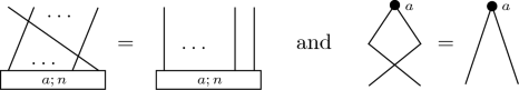
Area-dependent quantum field theory (aQFT¹) is a modification of 2-dimensional topological quantum field theory (TQFT): we consider the category of bordisms with area ${{\mathcal {B}}ord_2^{area}}$ and symmetric monoidal functors from it to the category of Hilbert spaces ${{\mathcal {H}}ilb}$ which depend continuously on the area. We can think of the area as a positive number attached to each connected component of a surface, additive under composition.² In order to have identities in ${{\mathcal {B}}ord_2^{area}}$, we allow zero area on cylinders.

The main change when passing from TQFTs to aQFTs, and indeed the main motivation to look at this generalisation in the first place, is that the state spaces can now be infinite-dimensional. This is in contrast to TQFTs, where dualisability forces all state spaces to be finite-dimensional (see e.g. [CR, Sec. 2.4]). The same argument for aQFTs merely requires each state space to be a separable Hilbert space (cf. Lemma 2.9 and Theorem 3.5).

The main example of an aQFT is two-dimensional Yang–Mills theory for a compact semisimple Lie group G [Mig, Rus, Wit], in which case the Hilbert space assigned to a circle is $Cl^2(G)$, that is, square integrable class functions on G. We treat this example in detail in Sect. 5. Area-dependent theories in general have been considered in [Bru] and briefly in [Seg, Sec. 1.4] (see also [Bar, Sec. 4.5]). A construction of area-dependent theories using triangulations with equal triangle area has been given in [CTS].

Two-dimensional TQFTs are of course a special case of aQFT, namely they are aQFTs which are independent of the area parameters. Conversely one can show that if for all bordisms $\Sigma$ the zero area limit of ${\mathcal {Z}}(\Sigma )$ exists, then all state spaces ${\mathcal {Z}}(U)$ are necessarily finite dimensional, and the zero area limit of ${\mathcal {Z}}$ is a TQFT (Remark 3.6).

Recall that 2d TQFTs are in one-to-one correspondence to commutative Frobenius algebras [Dij, Abr], and that there is a state sum construction of 2d TQFTs which starts from a strongly separable symmetric (not necessarily commutative) Frobenius algebra A as an input [BP, FHK, LP]. The commutative Frobenius algebra defining the TQFT obtained from this state sum construction is just the centre Z(A).

The generalisation of these results to aQFTs is for the most part straightforward to the point of being mechanical: just add a positive real parameter to all maps in sight (“area parameters”) and impose the condition that everything just depends on the sum of these areas.

The algebraic cornerstone of this work is the notion of a regularised Frobenius algebra (RFA), which consists of families of structure morphisms (product, unit, coproduct and counit), subject to the usual axioms of a Frobenius algebra, suitably decorated with area parameters (Definition 2.3).

An important example of an RFA is $L^2(G)$, the square integrable functions on a compact semisimple Lie group G. Here, the product $\mu _a$ and the coproduct $\Delta _a$ do have zero area limits given by the convolution product and by $\Delta _0(f)(g,h) := f(gh)$. The unit $\eta _a$ and counit $\varepsilon _a$ on the other hand do not have $a\rightarrow 0$ limits, see Sect. 5.1 for details. By the Peter-Weyl theorem we have $L^2(G) = \bigoplus _{V \in {\widehat{G}}} V \otimes V^*$, where the sum is a Hilbert space direct sum over isomorphism classes of irreducible unitary representations of G, and the RFA structure on $L^2(G)$ restricts to an infinite direct sum of finite-dimensional RFAs on $V \otimes V^*$. This is a general result for Hermitian RFAs, i.e. RFAs for which $\mu _a^\dagger = \Delta _a$ and $\eta _a^\dagger = \varepsilon _a$ for every $a\in {\mathbb {R}}_{>0}$ (Theorem 2.19):

Theorem 1.1

Every Hermitian RFA is a Hilbert space direct sum of finite dimensional Hermitian RFAs.

All examples of non-hermitian RFAs we know are also direct sums of finite dimensional RFAs, but we are not aware of a proof that this holds in general (Remark 2.17).

Finite dimensional RFAs in turn are very simple: they are just usual Frobenius algebras A together with an element H in the centre Z(A) of A, and the area-dependence is obtained by exponentiating H (Corollary 2.15). This makes RFAs sound not very interesting, but note that, conversely, an infinite direct sum of finite-dimensional RFAs has to satisfy non-trivial bounds to again define an RFA (Proposition 2.16). And as the example of $L^2(G)$ shows, the direct sum decomposition may not always be the most natural perspective.

Our next main theorem generalises the classification of 2d TQFTs in terms of commutative Frobenius algebras as given in [Dij, Abr]. Namely, in Theorem 3.5 (and in Corollary 3.7) we show:³

Theorem 1.2

There is a one-to-one correspondence between (Hermitian) aQFTs and (Hermitian) commutative RFAs.

In Sect. 4.2 we furthermore generalise the state sum construction of [BP, FHK, LP]. We find that a strongly separable symmetric RFA A (as defined in Sect. 2.1) provides—under one extra technical assumption—the data for the state sum construction of an aQFT, and the resulting aQFT corresponds, via Theorem 1.2, to the commutative RFA given by the centre of A.

This paper is organized as follows. In Sect. 2 we collect the algebraic preliminaries about RFAs, in Sect. 3 we state the definition of an aQFT and we show that aQFTs correspond to commutative RFAs. Section 4 contains the state sum construction and in Sect. 5 we give a detailed treatment of our main example, 2d YM theory.

2 Regularised Frobenius Algebras

In this section we study an algebraic notion—regularised Frobenius algebras—that will play a central role in characterising and producing examples of area-dependent QFTs. A more detailed treatment of this subject can be found in [Sze] where we also refer the reader for proofs that are omitted here. We denote with ${{\mathcal {H}}ilb}$ the category of Hilbert spaces and bounded linear maps with the strong operator topology on the hom sets ${{\mathcal {H}}ilb}({\mathcal {H}},{\mathcal {K}})={\mathcal {B}}({\mathcal {H}},{\mathcal {K}})$.

2.1 Definition of regularised algebras and Frobenius algebras

Definition 2.1

A regularised algebra is an object $A\in {{\mathcal {H}}ilb}$ together with continuous families of morphisms

$$\begin{aligned} \mu _a\in {\mathcal {B}}( A^{\otimes 2}, A)\quad \text {and}\quad \eta _a\in {\mathcal {B}}({\mathbb {C}}, A) \end{aligned}$$

(2.1)

for every $a\in {\mathbb {R}}_{>0}$, called product and unit, such that the following relations hold:

• 1. for every $a,a_1,a_2,b_1,b_2\in {\mathbb {R}}_{>0}$, such that $a_1+a_2=b_1+b_2$,

  $$\begin{aligned} \mu _{a_1}\circ \left( {{\,\mathrm{id}\,}}_{A}\otimes \eta _{a_2} \right)&=\mu _{b_1}\circ \left( \eta _{b_2}\otimes {{\,\mathrm{id}\,}}_{A}\right) , \end{aligned}$$

  (2.2)
  $$\begin{aligned} \mu _{a_1}\circ \left( {{\,\mathrm{id}\,}}_{A}\otimes \mu _{a_2} \right)&=\mu _{b_1}\circ \left( \mu _{b_2}\otimes {{\,\mathrm{id}\,}}_{A}\right) . \end{aligned}$$

  (2.3)

• 2. Let $P_a \in {\mathcal {B}}(A,A)$ be given by (2.2), i.e. $P_a = \mu _{a_1}\circ \left( id_{A}\otimes \eta _{a_2} \right)$ with $a=a_1+a_2$. We require that $\lim _{a\rightarrow 0}P_a={{\,\mathrm{id}\,}}_A$.

Let $A,B\in {{\mathcal {H}}ilb}$ be regularised algebras. A morphism of regularised algebras $A\xrightarrow {f}B$ is a morphism in ${{\mathcal {H}}ilb}$ such that for every $a\in {\mathbb {R}}_{>0}$

$$\begin{aligned} \eta ^{B}_a=f\circ \eta ^{A}_a,&\quad \mu ^{B}_a\circ \left( f\otimes f \right) =f\circ \mu _{a}^{A}. \end{aligned}$$

Instead of continuity of $\mu _a$ and $\eta _a$ in (2.1) it is enough to require continuity of $a\mapsto P_a$, for details see [Sze, Sec. 4.1.1]. On the other hand, it is important not to impose the existence of an $a\rightarrow 0$ limit on $\mu _a$ and $\eta _a$; in Sect. 2.4 we will see examples where this limit does not exist, which would then have been excluded.

Fig. 1

Graphical notation of morphisms in the symmetric monoidal category ${{\mathcal {H}}ilb}$. Here a morphism $f\in {\mathcal {B}}(A\otimes B,C\otimes D\otimes E)$, the identity ${{\,\mathrm{id}\,}}_{A}\in {\mathcal {B}}(A,A)$ and the symmetric braiding $\sigma _{A,B}$ are shown. The tensor product of morphisms is depicted by drawing the morphisms next to each other and composition of morphisms is stacking them on top of each other

We will often use string diagram notation to represent morphisms in ${{\mathcal {H}}ilb}$, our conventions are given in Fig. 1. The morphisms in (2.1) are drawn as

(2.4)

and the relations in (2.2) and (2.3) are

(2.5)

The next lemma gives some simple consequences of the above definition.

Lemma 2.2

Let A be a regularised algebra. Let $a_1,a_2,b_1,b_2,c_1,c_2\in {\mathbb {R}}_{>0}$ such that $a_1+a_2=b_2+b_2=c_1+c_2$.

• 1. Let $\eta _a'\in {\mathcal {B}}({\mathbb {C}},A)$ be a family of morphisms which satisfy (2.2) and Condition 2 of Definition 2.1. Then $\eta _a'=\eta _a$ for every $a\in {\mathbb {R}}_{>0}$.

• 2. $P_{a_1}\circ \eta _{a_2}=\eta _{a_1+a_2}$ and $P_{a_1}\circ P_{a_2}=P_{a_1+a_2}$.

• 3. $P_{a_1}\circ \mu _{a_2}=\mu _{b_1}\circ \left( P_{b_2}\otimes {{\,\mathrm{id}\,}}\right) =\mu _{c_1}\circ \left( {{\,\mathrm{id}\,}}\otimes P_{c_2}\right) =\mu _{a_1+a_2}$.

Proof

Here we only give the proof of Part 1, the proof of Part 2 and 3 are similar.

Let $a,b,c\in {\mathbb {R}}_{>0}$ and let us write $P'_{a+b}:=\mu _a\circ \left( \eta _b'\otimes {{\,\mathrm{id}\,}}_A \right)$ for the morphism in (2.2). From (2.2) we have that

$$\begin{aligned} \mu _{a}\circ \left( \eta _b\otimes \eta _c' \right) =\mu _{a}\circ \left( \eta _c\otimes \eta _b' \right) \end{aligned}$$

(2.6)

as both sides only depend on the sum of the parameters. We then have that

$$\begin{aligned} P_{a+b}\circ \eta _c'=P'_{a+b}\circ \eta _c, \end{aligned}$$

(2.7)

and using that the composition is separately continuous together with $\lim _{a,b\rightarrow 0}P_{a+b}=\lim _{a,b\rightarrow 0}P'_{a+b}={{\,\mathrm{id}\,}}_A$ we get that $\eta _c'=\eta _c$ for every $c\in {\mathbb {R}}_{>0}$.

$\square$

Next we introduce the dual concept to a regularised algebra. A regularised coalgebra is an object $A\in {{\mathcal {H}}ilb}$ together with continuous families of morphisms

$$\begin{aligned} \Delta _a: A\rightarrow A^{\otimes 2}\quad \text {and}\quad \varepsilon _a:A\rightarrow {\mathbb {C}} \end{aligned}$$

(2.8)

for $a\in {\mathbb {R}}_{>0}$, called coproduct and counit, such that the following relations hold: for all $a,a_1,a_2,b_1,b_2>0$, such that $a_1+a_2=b_1+b_2=a$,

$$\begin{aligned} \left( id_{A}\otimes \varepsilon _{a_2} \right) \circ \Delta _{a_1}&=\left( \varepsilon _{b_2}\otimes id_{A}\right) \circ \Delta _{b_1}=:P'_a, \end{aligned}$$

(2.9)

$$\begin{aligned} \left( id_{A}\otimes \Delta _{a_2} \right) \circ \Delta _{a_1}&=\left( \Delta _{b_2}\otimes id_{A}\right) \circ \Delta _{b_1}, \end{aligned}$$

(2.10)

and $\lim _{a\rightarrow 0}P'_a={{\,\mathrm{id}\,}}_A$. A morphism of regularised coalgebras, is a morphism of the objects which is compatible with $\Delta _a$ and $\varepsilon _a$ in the obvious way. Note that for a regularised coalgebra the dual statements of Lemma 2.2 hold. For the morphisms in (2.8) we introduce the following graphical notation:

(2.11)

A key notion in this paper is the following:

Definition 2.3

A regularised Frobenius algebra (or RFA in short) is a regularised algebra $A\in {{\mathcal {H}}ilb}$, which is also a regularised coalgebra, such that

(2.12)

holds for all $a_1+a_2=b_1+b_2=c_1+c_2$. A morphism of RFAs, is a morphism of regularised algebras and coalgebras.

In an RFA $P_a$ from the algebra structure and $P_a'$ from the coalgebra structure coincide:

Lemma 2.4

For an RFA we have $P_a=P'_a$ for all $a>0$.

Proof

Let $a,b \in {\mathbb {R}}_{>0}$ be arbitrary. Choose $a_1,a_2,b_2,b_2\in {\mathbb {R}}_{>0}$ such that $a=a_1+a_2$, $b=b_1+b_2$ and $a>b_1$ and $b>a_1$ (e.g. $b_1 = \frac{a}{2}$, $a_1= \frac{b}{2}$). By relation (2.12) one has that

$$\begin{aligned} \left( \mu _{a_2}\otimes {{\,\mathrm{id}\,}}_A \right) \circ \left( {{\,\mathrm{id}\,}}_A \otimes \Delta _{b_2}\right) =\Delta _{a_1+a_2-b_1}\circ \mu _{b_1+b_2-a_1}. \end{aligned}$$

(2.13)

Composing (2.13) with ${{\,\mathrm{id}\,}}_A\otimes \varepsilon _{b_1}$ from the left and with $\eta _{a_1}\otimes {{\,\mathrm{id}\,}}_A$ from the right yields

$$\begin{aligned} P_a\circ P'_b=P'_a\circ P_b. \end{aligned}$$

(2.14)

We can take the $b\rightarrow 0$ limit on both sides of (2.14) and use separate continuity of the composition to get $P_a=P'_a$. $\square$

We will prove the following lemma in “Appendix 5.2”.

Lemma 2.5

In the monoidal sub-category of ${{\mathcal {H}}ilb}$ tensor generated by an RFA and its structure morphisms every morphism is jointly continuous in the parameters.

This lemma is not entirely immediate as composition in ${{\mathcal {H}}ilb}$ is only separately continuous but not jointly continuous in the strong operator topology, and e.g. the map ${\mathcal {B}}(H,H) \rightarrow {\mathcal {B}}(K\otimes H,K\otimes H)$, $f \mapsto {{\,\mathrm{id}\,}}\otimes f$, is not continuous if K, H are infinite dimensional.

Remark 2.6

Usual (non-regularised) Frobenius algebras have an equivalent characterisation via a non-degenerate invariant pairing. The same is true in the regularised setting, however as we will not need it here, we only refer the reader to [Sze].

Recall the symmetric braiding $\sigma$ on ${{\mathcal {H}}ilb}$. We call a regularised algebra $A\in {{\mathcal {H}}ilb}$ commutative if $\mu _a\circ \sigma _{A,A}=\mu _a$ for all $a\in {\mathbb {R}}_{>0}$. The centre of a regularised algebra A is an object $B\in {{\mathcal {H}}ilb}$ and a morphism $i_B:B\rightarrow A$ such that

$$\begin{aligned} \mu _a\circ \sigma _{A,A} \circ \left( i_B \otimes {{\,\mathrm{id}\,}}_A \right) = \mu _a\circ \left( i_B \otimes {{\,\mathrm{id}\,}}_A \right) \end{aligned}$$

(2.15)

for all $a\in {\mathbb {R}}_{>0}$, which is universal in the following sense. If there is an object C and a morphism $f:C\rightarrow A$ satisfying the above equation then there is a unique morphism ${\tilde{f}}:C\rightarrow B$ such that the diagram

commutes. This implies in particular that $i_B$ is mono [Dav].

Lemma 2.7

The centre of a regularised algebra exists and it is a commutative regularised algebra.

Proof

One quickly checks that the closed subspace

$$\begin{aligned} K:=\bigcap _{\begin{array}{c} a\in {\mathbb {R}}_{>0}\\ x\in A \end{array}}\ker \left( \mu _a(x\otimes -)-\mu _a(-\otimes x)\right) \subseteq A \end{aligned}$$

(2.17)

satisfies (2.15). It satisfies the universal property (2.16) as any map $f:C\rightarrow A$ satisfying (2.15) lands in K.

Analogously to ordinary algebras we obtain induced product and unit morphisms on K satisfying the algebraic conditions (2.2) and (2.3). Finally, that the map ${\tilde{P}}_{a}$ induced by $P_a\circ i_K=i_K\circ {\tilde{P}}_a$ satisfies $\lim _{a\rightarrow 0} {{\tilde{P}}}_a = {{\,\mathrm{id}\,}}_K$ follows from taking the $a\rightarrow 0$ limit on both sides of the defining equation and using that $i_K$ is an isometric embedding. $\square$

A regularised algebra is separable if there exists a family of morphisms $e_a\in {\mathcal {B}}({\mathbb {C}},A\otimes A)$ for every $a\in {\mathbb {R}}_{>0}$ such that for $a_1+a_2=b_1+b_2=a$,

• 1. $(\mu _{a_1}\otimes {{\,\mathrm{id}\,}}_A)\circ ({{\,\mathrm{id}\,}}_A\otimes e_{a_2})=({{\,\mathrm{id}\,}}_A\otimes \mu _{b_1})\circ (e_{b_2}\otimes {{\,\mathrm{id}\,}}_A)$ and

• 2. $\mu _{a_1}\circ e_{a_2}=\eta _a$.

The $e_a$ are called separability idempotents. A regularised algebra A is strongly separable if it is separable and furthermore

• 3. $\sigma _{A,A}\circ e_a=e_a$.

These notions are direct generalisations of separability and strong separability for algebras, see e.g. [Kan, LP].

For an RFA A, we call the family of morphisms $\tau _{a}:=\mu _{a_1}\circ \Delta _{a_2}\circ \eta _{a_3}$ for $a_1,a_2,a_3\in {\mathbb {R}}_{>0}$ with $a=a_1+a_2+a_3$ the window element of A, cf. [LP, Def. 2.12]. We call the window element invertible if there exists a family of morphisms $z_a\in {\mathcal {B}}({\mathbb {C}},A)$ for $a\in {\mathbb {R}}_{>0}$ (the inverse) such that $\mu _{a_1}\circ (\tau _{a_2}\otimes z_{a_3})=\eta _{a_1+a_2+a_3} = \mu _{a_1}\circ (z_{a_3}\otimes \tau _{a_3})$. From a direct computation one can verify that if there exists another family of morphisms $z'_a$ which satisfies the above equation then $z'_a=z_a$ for every $a\in {\mathbb {R}}_{>0}$, that is the inverse of the window element is unique. In the following we write $\tau ^{-1}_a$ for the inverse of $\tau _a$. It is easy to check that the window element and its inverse satisfy (2.15).

An RFA is symmetric if $\varepsilon _{a_1}\circ \mu _{a_2}\circ \sigma =\varepsilon _{b_1}\circ \mu _{b_2}$. The following is a direct translation of [LP, Thm. 2.14] for strong separability for symmetric Frobenius algebras.

Proposition 2.8

A symmetric RFA is strongly separable if and only if its window element is invertible.

Proof

Set $e_a:=\Delta _{a_1}\circ \tau ^{-1}_{a_2}$. Conversely set $\tau ^{-1}_a:=(\varepsilon _{a_1}\otimes {{\,\mathrm{id}\,}}_A)\circ e_{a_2}$. $\square$

2.2 Properties of RFAs

In this section we collect some properties of RFAs. The next lemma shows in particular that an RFA has a Hilbert basis with at most countably many elements.

Lemma 2.9

Let A be an RFA.

• 1. The Hilbert space underlying A is separable.

• 2. For all $a\in {\mathbb {R}}_{>0}$, $P_a$ is a trace class operator (and hence compact).

Proof

Part 1: Let be a complete set of orthonormal vectors in A and write $\gamma _{a}(1):=\Delta _{a_1}\circ \eta _{a_2}(1)=\sum _{k,l\in I}\phi _k\otimes \phi _l\,\gamma _{a}^{kl}$ with $a=a_1+a_2$. By [Kub, Cor. 5.28], independently of the countability of the indexing set I, there are at most countably many non-zero terms in the above sum. Thus for a given $a\in {\mathbb {R}}_{>0}$ there is a countable set of pairs $(k,l) \in I \times I$ such that $\gamma _{a}^{kl}\ne 0$. Define $I(a)\subseteq I$ to be the countable set of all elements of I that appear in such a pair. Let

(2.18)

Note that J is countable and $A_J$ is separable. Write $\beta _{a}:=\varepsilon _{a_1}\circ \mu _{a_2}$. By (2.12), this satisfies

$$\begin{aligned} ({{\,\mathrm{id}\,}}_A\otimes \beta _{a_1})\circ (\gamma _{a_2}\otimes {{\,\mathrm{id}\,}}_A)=P_{a} \end{aligned}$$

(2.19)

and hence for every $v\in A$ and $n\in {\mathbb {Z}}_{>0}$ we have that

$$\begin{aligned} P_{1/n}(v)\in A_J\quad \text { and }\quad \lim _{n\rightarrow \infty }P_{1/n}(v)=v, \end{aligned}$$

(2.20)

since $\lim _{n\rightarrow \infty }P_{1/n}={{\,\mathrm{id}\,}}_A$ in the strong operator topology. Since $A_J$ is closed, v is an element of $A_J$. We have shown that $A_J=A$, and hence that A is separable.

Part 2: First let us compute the following expression for some $a_1,a_2\in {\mathbb {R}}_{>0}$:

$$\begin{aligned} \beta _{a_1}\circ \sigma \circ \gamma _{a_2}(1) =\sum _{j,k\in I}\beta _{a_1}(\phi _j\otimes \phi _k)\gamma _{a_2}^{kj} . \end{aligned}$$

(2.21)

This is an absolutely convergent sum, since the left hand side is a composition of bounded linear maps. We can rewrite this expression using (2.19) to get

$$\begin{aligned} \begin{aligned} \beta _{a_1}\circ \sigma \circ \gamma _{a_2}(1)&=\sum _{j,k,l\in I}\beta _{a_1}(\phi _j\otimes \phi _k)\gamma _{a_2}^{kl} \langle \phi _j|\phi _l\rangle \\&=\sum _{j,k,l\in I}\langle \phi _j|(\beta _{a_1}\otimes {{\,\mathrm{id}\,}}_A)\phi _j\otimes \phi _k\otimes \phi _l \gamma _{a_2}^{kl}\rangle \rangle \\&=\sum _{j\in I}\langle \phi _j|(\beta _{a_1}\otimes {{\,\mathrm{id}\,}}_A)\phi _j\otimes \sum _{k,l\in I}\phi _k\otimes \phi _l \gamma _{a_2}^{kl}\rangle \rangle \\&=\sum _{j\in I}\langle \phi _j|(\beta _{a_1}\otimes {{\,\mathrm{id}\,}}_A) \circ ({{\,\mathrm{id}\,}}_A\otimes \gamma _{a_2}(1))\phi _j\rangle \\&=\sum _{j\in I}\langle \phi _j|P_a\phi _j\rangle , \end{aligned} \end{aligned}$$

(2.22)

which is again an absolutely convergent sum. By [Con2, Ex. 18.2] $P_a$ is a trace class operator if and only if $\sum _{j\in I}\langle \phi _j|P_a\phi _j\rangle$ is absolutely convergent for every choice of orthonormal basis $\{ \phi _j \}$, which we just have shown. In this case we have that

$$\begin{aligned} {{\,\mathrm{tr}\,}}(P_a)=\sum _{j\in I}\langle \phi _j|P_a\phi _j\rangle . \end{aligned}$$

(2.23)

$\square$

Let $A\in {{\mathcal {H}}ilb}$ be an RFA. By the Part 2 of Lemma 2.9 and [EN, Thm. II.4.29], $a\mapsto P_a$ (for $a>0$) is norm continuous. The following corollary shows that if we had defined ${{\mathcal {H}}ilb}$ to have the norm operator topology on hom-sets all examples of RFAs with self-adjoint $P_a$ would be finite-dimensional.

Corollary 2.10

Let $A\in {{\mathcal {H}}ilb}$ be an RFA such that $\lim _{a\rightarrow 0}P_a={{\,\mathrm{id}\,}}_A$ in the norm topology on ${\mathcal {B}}(A)$. Then A is finite-dimensional.

Proof

From Lemma 2.9 (2) we know that $P_a$ is compact for every $a\in {\mathbb {R}}_{>0}$. By [Con1, Prop. VI.3.4] the subspace of compact operators is closed in norm operator topology. These together with $\lim _{a\rightarrow 0}P_a={{\,\mathrm{id}\,}}_A$ imply that ${{\,\mathrm{id}\,}}_A$ is compact, which in turn implies that A is finite-dimensional. $\square$

We denote the category of RFAs by ${\mathcal {RF}rob}$ and its subcategory of commutative RFAs by ${c\mathcal {RF}rob}$.

Proposition 2.11

Any morphism in ${\mathcal {RF}rob}$ is mono and epi.

Proof

Let $\varphi :A\rightarrow B$ be a morphism of RFAs and let $\psi _{a,b}:=({{\,\mathrm{id}\,}}_A\otimes \beta _b^B)\circ ({{\,\mathrm{id}\,}}_A\otimes \varphi \otimes {{\,\mathrm{id}\,}}_B)\circ (\gamma _a^A\otimes {{\,\mathrm{id}\,}}_B)$. Then $\varphi \circ \psi _{a,b}=P_{a+b}^B$ and $\psi _{a,b}\circ \varphi =P_{a+b}^A$. We show that $\varphi$ is epi, showing that it is mono is similar. Let $f,g\in {\mathcal {B}}(B,X)$ for an object X such that $f\circ \varphi =g\circ \varphi$. After composing with $\psi _{a,b}$ from the right for $a,b\in {\mathbb {R}}_{>0}$ we get $f\circ P^B_{a+b}=g\circ P^B_{a+b}$. This last equation holds for every $a,b\in {\mathbb {R}}_{>0}$, so we can take the limit $a,b\rightarrow 0$ to get $f=g$. $\square$

Remark 2.12

As we will see in Example 2 in Sect. 2.4, not every morphism of RFAs is invertible, hence ${\mathcal {RF}rob}$ is not a groupoid.

For $A,B\in {\mathcal {RF}rob}$ the object $A\otimes B$ is an RFAs by

$$\begin{aligned} \begin{aligned} \mu _{a}^{A\otimes B}&:=\left( \mu _a^A\otimes \mu _a^B \right) \circ \left( {{\,\mathrm{id}\,}}\otimes \sigma \otimes {{\,\mathrm{id}\,}}\right) ,&\eta _a^{A\otimes B}&:=\eta _a^A\otimes \eta _a^B,\\ \Delta _a^{A\otimes B}&:=\left( {{\,\mathrm{id}\,}}\otimes \sigma \otimes {{\,\mathrm{id}\,}}\right) \circ \left( \Delta _a^A\otimes \Delta _a^B \right) ,&\varepsilon _a^{A\otimes B}&:=\varepsilon _a^A\otimes \varepsilon _a^B. \end{aligned} \end{aligned}$$

(2.24)

Proposition 2.13

${\mathcal {RF}rob}$ is a symmetric monoidal category with the above tensor product.

Recall that a Frobenius algebra in ${{\mathcal {H}}ilb}$ is always finite-dimensional see e.g. [Koc, Prop. 2.3.24].

Proposition 2.14

Let $A\in {\mathcal {RF}rob}$. The following are equivalent.

• 1. A is finite-dimensional.

• 2. All of the following limits exist:

  $$\begin{aligned} {\lim }_{a\rightarrow 0}\eta _a , \quad {\lim }_{a\rightarrow 0}\mu _a , \quad {\lim }_{a\rightarrow 0}\varepsilon _a , \quad {\lim }_{a\rightarrow 0}\Delta _a . \end{aligned}$$

Proof

($1\Rightarrow 2$): If A is finite-dimensional, then the map $a\mapsto P_a$ is norm continuous, hence $P_a=e^{aH}$ for some $H\in {\mathcal {B}}(A)$. Then $\eta _0:=e^{-aH}\eta _a$ is independent of a and $\eta _a=P_a \circ \eta _0$, hence $\lim _{a\rightarrow 0}\eta _a=\eta _0$ exists. One similarly proves that the other limits exist as well.

($1\Leftarrow 2$): The morphisms given by these limits define a Frobenius algebra structure on A, hence A is finite-dimensional. $\square$

Corollary 2.15

A finite dimensional RFA A is in fact an ordinary Frobenius algebra $A^{(0)}$ together with an element in its centre $H\in Z(A^{(0)})$ which one obtains by differentiating $P_a$ at $a=0$. Conversely, the area depenence on $A^{(0)}$ can be restored by setting $P_a:=e^{aH}$.

For more details on this, see [Sze, Sec. 4.1.4].

Proposition 2.16

Let I be a countable (possibly infinite) set. For $k\in I$ let $F_k\in {{\mathcal {H}}ilb}$ be a (possibly infinite-dimensional) RFA. Then $\bigoplus _{k\in I}F_k$ (the completed direct sum of Hilbert spaces) is an RFA if and only if, for every $a\in {\mathbb {R}}_{>0}$,

$$\begin{aligned} \sup _{k\in I} \left\| {\mu _a^k}\right\|<\infty \quad&\text {and}\quad \sup _{k\in I} \left\| {\Delta _a^k}\right\| <\infty , \end{aligned}$$

(2.25)

$$\begin{aligned} \sum _{k\in I} \left\| {\varepsilon _a^k}\right\| ^2<\infty \quad&\text {and}\quad \sum _{k\in I} \left\| {\eta _a^k}\right\| ^2<\infty , \end{aligned}$$

(2.26)

where $\mu _a^k$, $\Delta _a^k$, $\varepsilon _a^k$ and $\eta _a^k$ denote the structure maps of $F_k$.

Proof

Let $F:=\bigoplus _{k\in I}F_k$ and fix the value of a.

($\Rightarrow$): Let us write $x_k$ for the k’th component of $x\in F=\bigoplus _{k\in I}F_k$. Then for every $k\in I$

$$\begin{aligned} \left\| {\Delta _a^k}\right\| =\sup _{\begin{array}{c} x_k\in F_k\\ \left\| {x_k}\right\| =1 \end{array}} \left\| {\Delta _a^k(x_k)}\right\| = \sup _{\begin{array}{c} x_k\in F_k\\ \left\| {x_k}\right\| =1 \end{array}} \left\| {\Delta _a(x_k)}\right\| \le \sup _{\begin{array}{c} x_k\in F_k\\ \left\| {x_k}\right\| =1 \end{array}} \left\| {\Delta _a}\right\| \cdot \left\| {x_k}\right\| = \left\| {\Delta _a}\right\| <\infty , \end{aligned}$$

so in particular $\sup _{k} \left\| {\Delta _a^k}\right\| <\infty$. A similar proof applies to the case of $\mu _a$. We calculate the norm of $\eta _a$:

$$\begin{aligned} \left\| {\eta _a}\right\| ^2= \left\| {\eta _a(1)}\right\| ^2=\sum _{k\in I} \left\| {\eta _a^k(1)}\right\| ^2=\sum _{k\in I} \left\| {\eta _a^k}\right\| ^2, \end{aligned}$$

which is finite if and only if $\eta _a$ is a bounded operator. If $\varepsilon _a$ is bounded, then by the Riesz Lemma there exists a unique $v\in F$ such that $\varepsilon _a(x)=\langle v,x\rangle$ and $\left\| {\varepsilon _a}\right\| = \left\| {v}\right\|$. Then $\langle v_k,x_k\rangle =\langle v,x_k\rangle =\varepsilon _a(x_k)=\varepsilon _a^k(x_k)$. So again by the Riesz Lemma $\left\| {\varepsilon _a^k}\right\| = \left\| {v_k}\right\|$. We have that

$$\begin{aligned} \left\| {\varepsilon _a}\right\| ^2= \left\| {v}\right\| ^2=\sum _{k\in I} \left\| {v_k}\right\| ^2=\sum _{k\in I} \left\| {\varepsilon _a^k}\right\| ^2. \end{aligned}$$

($\Leftarrow$): The operators $\eta _a$ and $\varepsilon _a$ are bounded by the previous discussion. For $\Delta _a$ one has that

$$\begin{aligned} \left\| {\Delta _a}\right\| ^2&= \sup _{\begin{array}{c} x\in F\\ \left\| {x}\right\| =1 \end{array}} \left\| {\Delta _a(x)}\right\| ^2= \sup _{\begin{array}{c} x\in F\\ \left\| {x}\right\| =1 \end{array}} \left\| {\sum _{k\in I}\Delta _a(x_k)}\right\| ^2= \sup _{\begin{array}{c} x\in F\\ \left\| {x}\right\| =1 \end{array}}\sum _{k\in I} \left\| {\Delta ^k_a(x_k)}\right\| ^2\\ {}&\le \sup _{\begin{array}{c} x\in F\\ \left\| {x}\right\| =1 \end{array}}\sum _{k\in I} \left\| {\Delta ^k_a}\right\| ^2 \left\| {x_k}\right\| ^2 \le \left( \sup _{l} \left\| {\Delta _a^l}\right\| ^2\right) \cdot \sup _{\begin{array}{c} x\in F\\ \left\| {x}\right\| =1 \end{array}}\sum _{k\in I} \left\| {x_k}\right\| ^2= \sup _{l} \left\| {\Delta _a^l}\right\| ^2<\infty , \end{aligned}$$

so $\Delta _a$ is bounded. For $\mu _a$ the proof is similar.

Then one needs to check that $a\mapsto P_a:=\sum _{k\in I}P_a^k$ is continuous. Let $\varepsilon \in {\mathbb {R}}_{>0}$, $a_0\in {\mathbb {R}}_{\ge 0}$ and $f\in \bigoplus _{k\in I}F_k$ with components $f_k$ be fixed. Let $a'>a_0$ and $0<E<\varepsilon$ be arbitrary. Since $P_a-P_{a_0}$ is a bounded operator, one can find $J_{a'}\subset I$ finite, such that for every $a<a'$

$$\begin{aligned} \sum _{j\in I{\setminus } J_{a'}} \left\| {(P_a^j-P_{a_0}^j)f_j}\right\| ^2<E. \end{aligned}$$

Then let $\delta '>0$ be such that for every $|a-a_0|<\delta '$

$$\begin{aligned} \sum _{j\in J_{a'}} \left\| {(P_a^j-P_{a_0}^j)f_j}\right\| ^2<\varepsilon -E, \end{aligned}$$

which can be chosen since the sum is finite and each $P_a^j$ is continuous by assumption. Finally let $\delta :=\mathrm {min}\left\{ \delta ',a'-a_0 \right\}$. By construction we have that for every $|a-a_0|<\delta$,

$$\begin{aligned} \left\| {(P_a-P_{a_0})f}\right\| ^2=\sum _{j\in I} \left\| {(P_a^j-P_{a_0}^j)f_j}\right\| ^2<\varepsilon . \end{aligned}$$

$\square$

Remark 2.17

All examples of RFAs known to us are of the form given in Proposition 2.16 with finite-dimensional summands $F_k$. In fact we can show from the statements in [BB, Sec. 6.4] that all RFAs are (not necessarily orthogonal) direct sums of finite dimensional RFAs and a direct summand, on which $P_a$ is quasinilpotent for every $a>0$. This summand may be either 0 or infinite dimensional. The finite dimensional summands are generalised eigenspaces of $P_a$ for every $a>0$, while the remaining factor is the intersection of their complement. On the latter $P_a$ is quasinilpotent for every $a>0$ by [BB, Cor. 7.2.4]. For Hermitian RFAs, which we will introduce in Sect. 2.3, we show that this direct summand is 0 (see the proof of Theorem 2.19). We do not know an example of an RFA where this summand is non-zero. Note also that the same RFA $F_k$ cannot appear infinitely many times, as otherwise the bounds (2.26) would be violated.

2.3 Classification of Hermitian RFAs

We start by recalling the notion of a dagger (or $\dagger$-) symmetric monoidal category ${\mathcal {S}}$, e.g. from [Sel]. A dagger structure on ${\mathcal {S}}$ is a functor $(-)^{\dagger }:{\mathcal {S}}\rightarrow {\mathcal {S}}^{opp}$ which is identity on objects, $(-)^{\dagger \dagger }={{\,\mathrm{id}\,}}_{{\mathcal {S}}}$, $(f\otimes g)^{\dagger }=f^{\dagger }\otimes g^{\dagger }$ for any morphisms f, g and $\sigma _{U,V}^{\dagger }=\sigma _{V,U}$. We fix the dagger structure on ${{\mathcal {H}}ilb}$ given by adjoints.

Definition 2.18

A Hermitian regularised Frobenius algebra (or $\dagger$-RFA for short) is an RFA for which $\mu _a^{\dagger }=\Delta _a$ and $\eta _a^{\dagger }=\varepsilon _a$ (and therefore $P_a=P_a^{\dagger }$). We denote by $\dagger \text {-}{\mathcal {RF}rob}$ the full subcategory of ${\mathcal {RF}rob}$ of $\dagger$-RFAs.

Let $\dagger \text {-}{{\mathcal {F}}rob^{\mathrm {F}}}$ denote the category which has objects countable families $\Phi =\left\{ F_j,\sigma _j \right\} _{j\in I}$ of $\dagger$-Frobenius algebras $F_j$ and real numbers $\sigma _j$, such that for every $a\in {\mathbb {R}}_{>0}$

$$\begin{aligned} \sup _{j\in I}\left\{ e^{-a\sigma _j} \left\| {\mu _j}\right\| \right\}<\infty \quad \text { and } \quad \sum _{j\in I}e^{-2a\sigma _j} \left\| {\eta _j}\right\| ^2<\infty . \end{aligned}$$

(2.27)

A morphism $\Psi :\Phi \rightarrow \Phi '$ consists of a bijection $f:I\xrightarrow {\sim }I'$ which satisfies $\sigma _j=\sigma _{f(j)}$ and a family of morphisms of Frobenius algebras $\psi _j:F_j\rightarrow F'_{f(j)}$ (which are automatically invertible [Koc, Lem. 2.4.5]). We will write $\Psi =\left( f,\left\{ \psi _j \right\} _{j\in I} \right)$.

Let $\Phi \in \dagger \text {-}{{\mathcal {F}}rob^{\mathrm {F}}}$ with the notation from above. For $j\in I$ we turn the Frobenius algebra $F_j$ into an RFA by multiplying its structure morphisms by $e^{-a\sigma _j}$. Using Proposition 2.16, we get an RFA structure on $\bigoplus _{j\in I}F_j$. The next theorem shows that the resulting functor is an equivalence.

Theorem 2.19

There is an equivalence of categories $\dagger \text {-}{{\mathcal {F}}rob^{\mathrm {F}}}\rightarrow \dagger \text {-}{\mathcal {RF}rob}$ given by $\Phi \mapsto \bigoplus _{j\in I}F_j$.⁴

Proof

We define the inverse functor. Let $F\in \dagger \text {-}{\mathcal {RF}rob}$ and fix $a\in {\mathbb {R}}_{>0}$. Then $P_a$ is self-adjoint and therefore can be diagonalised. Let $\mathrm {sp}_{\mathrm {pt}}(P_a)$ denote the point spectrum⁵ of $P_a$. Furthermore, by Lemma 2.9$P_a$ is of trace class, and hence compact. Thus it has at most countably many eigenvalues and the eigenspaces with non-zero eigenvalues are finite-dimensional. Let

$$\begin{aligned} F=\bigoplus _{\alpha \in \mathrm {sp}_{\mathrm {pt}}(P_a) }F_{\alpha } \end{aligned}$$

(2.28)

be the corresponding eigenspace decomposition of $P_a$.

Claim: The eigenvalue $\alpha$ of $P_a$ on $F_{\alpha }$ is of the form $e^{-a \sigma _{\alpha }}$ for some $\sigma _{\alpha }\in {\mathbb {R}}$. In particular 0 is not an eigenvalue.

To show this, first assume that $c(a):=\alpha \ne 0$, so that $F_{\alpha }$ is finite-dimensional, and simultaneously diagonalise $P_a$, $P_b$ and $P_{a+b}$ on $F_{\alpha }$. Then on a subspace where all three operators are constant with values c(a), c(b) and $c(a+b)$ one has that $c(a)c(b)=c(a+b)$. Furthermore $a\mapsto c(a)$ is a continuous function ${\mathbb {R}}_{\ge 0}\rightarrow {\mathbb {R}}$ and $c(0)=1$ since $a\mapsto P_a$ is strongly continuous at every $a\in {\mathbb {R}}_{\ge 0}$ and $\lim _{a\rightarrow 0}P_a={{\,\mathrm{id}\,}}_F$. So the unique solution to the above functional equation is $c(a)=e^{-a \sigma _{\alpha }}$ for some $\sigma _{\alpha }\in {\mathbb {R}}$.

Finally let us assume that $\alpha =0$. Clearly, $\ker (P_{a})\subseteq \ker (P_{a+b})$ for every $b\in {\mathbb {R}}_{\ge 0}$. Since $P_a$ is self-adjoint, we have for $v\in F_0$ that $0=P_a(v)=P_{a/2}^{\dagger }\circ P_{a/2}(v)$. But then $P_{a/2}(v)=0$ and similarly, for every $n\in {\mathbb {Z}}_{\ge 0}$ we have that $P_{a/2^n}(v)=0$. Altogether we have that $F_{0}=\ker (P_{a})=\ker (P_{b})$ for every $b\in {\mathbb {R}}_{\ge 0}$. So $\lim _{a\rightarrow 0}P_a={{\,\mathrm{id}\,}}_F$ implies that $F_0=\left\{ 0 \right\}$.

Claim: The eigenspaces are $\dagger$-Frobenius algebras by restricting and projecting the structure maps of F.

To show this, first confirm that the structure maps do not mix eigenspaces of $P_a$, because $P_a$ commutes with them. Then checking $\dagger$-RFA relations is straightforward and these are $\dagger$-Frobenius algebras, cf. Proposition 2.14.

Claim: The convergence conditions in (2.27) are satisfied by the above obtained family of $\dagger$-Frobenius algebras $F_{\alpha }$ and real numbers $\sigma _{\alpha }$.

This can be shown directly by computing the norm of the structure maps.

Showing that the two functors give an equivalence of categories is now straightforward. $\square$

Corollary 2.20

Let $A\in {{\mathcal {H}}ilb}$ be a $\dagger$-RFA. Then $P_a$ is mono and epi.

Proof

From the proof of Theorem 2.19 we see that $P_a$ is mono. Since $P_a$ is self-adjoint we get that $P_a$ is epi. $\square$

Lemma 2.21

• 1. Every $\dagger$-Frobenius algebra in ${{\mathcal {H}}ilb}$ is separable, hence semisimple.

• 2. Every $\dagger$-RFA is separable.

Proof

Part 1:

Let F denote a $\dagger$-Frobenius algebra in ${{\mathcal {H}}ilb}$ and let $\xi :=\mu \circ \Delta =\Delta ^{*}\circ \Delta$, which is an F-F-bimodule morphism and an F-F-bicomodule morphism. It is a self-adjoint operator, so it can be diagonalised and F decomposes into Hilbert spaces as

$$\begin{aligned} F=\bigoplus _{\alpha \in \mathrm {sp}(\xi )}F_{\alpha }, \end{aligned}$$

(2.29)

where $F_{\alpha }$ is the eigenspace of $\xi$ with eigenvalue $\alpha$.

Now we show that (2.29) is a direct sum of Frobenius algebras. Let $\alpha \ne \beta$ and take $a\in F_{\alpha }$, $b\in F_{\beta }$. We have

$$\begin{aligned} \begin{aligned} \xi (ab)&=a\xi (b)={\beta }ab\\&=\xi (a)b={\alpha }ab \end{aligned} \end{aligned}$$

(2.30)

since $\xi$ is a bimodule morphism. Then (2.30) shows that $ab=0$, so (2.29) is a decomposition as algebras.

Similarly one shows that (2.29) is a decomposition as coalgebras. We have for every $a\in F_{\alpha }$, using Sweedler notation:

$$\begin{aligned} \begin{aligned} \Delta (\xi (a))&=\xi (a_{(1)})\otimes a_{(2)}=a_{(1)}\otimes \xi (a_{(2)})\\&=\alpha \Delta (a)=\alpha a_{(1)} \otimes a_{(2)}, \end{aligned} \end{aligned}$$

(2.31)

which shows that the comultiplication restricted to $F_{\alpha }$ lands in $F_{\alpha }\otimes F_{\alpha }$.

We now show that 0 is not in the spectrum. Let us assume otherwise. Then $F_0$ is a Frobenius algebra. We have $\xi (x)=\Delta ^*\circ \Delta (x)=0$ for every $x\in F_0$, and so also $\Delta (x)=0$, which is a contradiction to counitality. Therefore 0 is not in the spectrum of $\xi$, i.e. $\xi$ is injective.

Now the only thing left to show is that each summand $F_{\alpha }$ is semisimple. Take $\Delta (1)\cdot \alpha ^{-1}$ projected on $F_{\alpha }\otimes F_{\alpha }$ and denote it by $e^{\alpha }$. This is a separability idempotent for the algebra $F_{\alpha }$, hence $F_{\alpha }$ is separable, hence semisimple (see e.g. [Pie, Ch. 10.4]).

Part 2:

By Theorem 2.19 we can decompose a $\dagger$-RFA $A=\bigoplus _{\sigma \in I}A_{\sigma }$ into $\dagger$-Frobenius algebras and by the above proof we can decompose the $A_{\sigma }$ summands into finite dimensional separable algebras $A_{\sigma }=\bigoplus _{\alpha } A_{\sigma ,\alpha }$ with separability idempotents $e^{\sigma ,\alpha }$. We have

$$\begin{aligned} \begin{aligned} \left\| {e^{\sigma ,\alpha }}\right\| ^2&= \left\| {\alpha ^{-1}\cdot \Delta ^{\sigma ,\alpha }(1)}\right\| ^2 {\mathop {=}\limits ^{(C^*)}} \left\| {\alpha ^{-2}\cdot \varepsilon ^{\sigma ,\alpha }\circ \mu ^{\sigma ,\alpha }\circ \Delta ^{\sigma ,\alpha }(1)}\right\| \\ {}&= \left\| {\alpha ^{-1}\cdot \varepsilon ^{\sigma ,\alpha }(1)}\right\| {\mathop {=}\limits ^{(C^*)}} \alpha ^{-1}\cdot \left\| {\eta ^{\sigma ,\alpha }}\right\| ^2, \end{aligned} \end{aligned}$$

(2.32)

where $(C^*)$ refers to the fact that $\left\| {X^{\dagger }X}\right\| = \left\| {X}\right\| ^2$ and in the middle step we used that $A_{\sigma ,\alpha }$ is the eigenspace of $\xi ^{\sigma }=\mu ^{\sigma }\circ \Delta ^{\sigma }$ with eigenvalue $\alpha$. Furthermore we have that

$$\begin{aligned} \begin{aligned} 1&= \left\| {{{\,\mathrm{id}\,}}_{A_{\sigma ,\alpha }}}\right\| ^2 = \left\| {\mu ^{\sigma ,\alpha }\circ (\eta ^{\sigma ,\alpha }\otimes {{\,\mathrm{id}\,}})}\right\| ^2\\&\le \left\| {\mu ^{\sigma ,\alpha }}\right\| ^2\cdot \left\| {\eta ^{\sigma ,\alpha }}\right\| ^2 {\mathop {=}\limits ^{(C^*)}} \left\| {\mu ^{\sigma ,\alpha }\circ \Delta ^{\sigma ,\alpha }}\right\| \cdot \left\| {\eta ^{\sigma ,\alpha }}\right\| ^2 =\alpha \cdot \left\| {\eta ^{\sigma ,\alpha }}\right\| ^2. \end{aligned} \end{aligned}$$

(2.33)

We claim that

$$\begin{aligned} e_a:=\sum _{\begin{array}{c} \sigma \in I\\ \alpha \in \mathrm {sp}(\xi ^{\sigma }) \end{array}} e^{-a\sigma } e^{\sigma ,\alpha }\in A\otimes A, \end{aligned}$$

(2.34)

which is then clearly a separability idempotent for the RFA A. To check (2.34) we compute

$$\begin{aligned} \begin{aligned} \left\| {e_a}\right\| ^2&=\sum _{\begin{array}{c} \sigma \in I\\ \alpha \in \mathrm {sp}(\xi ^{\sigma }) \end{array}} e^{-2a\sigma } \left\| {e^{\sigma ,\alpha }}\right\| ^2= \sum _{\begin{array}{c} \sigma \in I\\ \alpha \in \mathrm {sp}(\xi ^{\sigma }) \end{array}} e^{-2a\sigma } \alpha ^{-1} \left\| {\eta ^{\sigma ,\alpha }}\right\| ^2\\&{\mathop {\le }\limits ^{(2.33)}} \sum _{\begin{array}{c} \sigma \in I\\ \alpha \in \mathrm {sp}(\xi ^{\sigma }) \end{array}} e^{-2a\sigma } \left\| {\eta ^{\sigma ,\alpha }}\right\| ^4 \le \left\| {\eta _{a/2}}\right\| ^{4}<\infty . \end{aligned} \end{aligned}$$

(2.35)

$\square$

Let $\epsilon \in {\mathbb {C}}{\setminus }\left\{ 0 \right\}$, $\sigma \in {\mathbb {R}}$ and let ${\mathbb {C}}_{\epsilon ,\sigma }$ denote the one-dimensional $\dagger$-RFA structure on ${\mathbb {C}}$ given by

$$\begin{aligned} \begin{aligned} \varepsilon _a(1)&=e^{-a\sigma }\epsilon ,&\Delta _a(1)&=\frac{e^{-a\sigma }}{\epsilon }1\otimes 1,&\eta _a(1)&=e^{-a\sigma } \epsilon ^* 1,&\mu _a(1\otimes 1)&=\frac{e^{-a\sigma }}{\epsilon ^*}1. \end{aligned} \end{aligned}$$

(2.36)

Let $C\in {{\mathcal {H}}ilb}$ be a one-dimensional $\dagger$-RFA and $c\in C$ with $\left\| {c}\right\| =1$. Then by Proposition 2.14, $\varepsilon _a=\varepsilon _0\circ P_a$ with $P_a=e^{-a\sigma } {{\,\mathrm{id}\,}}_C$ for $\sigma \in {\mathbb {R}}$. Set $\epsilon :=\varepsilon _0(c)\in {\mathbb {C}}$. Then

$$\begin{aligned} \begin{aligned} C&\rightarrow {\mathbb {C}}_{\epsilon ,\sigma }\\ c&\mapsto 1 \end{aligned} \end{aligned}$$

(2.37)

is an isometric isomorphism of RFAs.

Corollary 2.22

Let C be a commutative $\dagger$-RFA. Then there is a family of numbers $\left( \epsilon _j,\sigma _j \right) _{j\in I}$, where $\epsilon _j\in {\mathbb {C}}$ and $\sigma _j\in {\mathbb {R}}$, satisfying

$$\begin{aligned} \sup _{j\in I}\left\{ e^{-a\sigma _j}|\epsilon _j|^{-1} \right\}<\infty \quad \text{ and } \quad \sum _{j\in I}e^{-2a\sigma _j}|\epsilon _j|^2<\infty \end{aligned}$$

(2.38)

for every $a\in {\mathbb {R}}_{>0}$ such that $C\cong \bigoplus _{j\in I}{\mathbb {C}}_{\epsilon _j,\sigma _j}$ as RFAs.

Proof

By Theorem 2.19 and Lemma 2.21, C is a direct sum of semisimple algebras. By the Wedderburn-Artin theorem every semisimple commutative algebra is a direct sum of one-dimensional algebras. Using the isomorphism (2.37) we get the above family of numbers. The finiteness conditions come from (2.27). $\square$

Lemma 2.23

Let $\varphi :{\mathbb {C}}_{\epsilon ,\sigma }\rightarrow {\mathbb {C}}_{\epsilon ',\sigma '}$ be a morphism of RFAs. Then $\varphi (1)=\epsilon /\epsilon '\in U(1)$ and $\sigma =\sigma '$.

Proof

From $\varphi \circ \eta _a=\eta _a'$ one has that for every $a\in {\mathbb {R}}_{\ge 0}$, $\varphi (1)\epsilon ^* e^{-a\sigma }= (\epsilon ')^* e^{-a\sigma '}$. Since $\epsilon \ne 0$, $\epsilon '\ne 0$ and $\varphi (1)\ne 0$, one must have $\sigma =\sigma '$ and hence $\varphi (1)\epsilon ^* = (\epsilon ')^*$. One similarly obtains from $\varepsilon '_a\circ \varphi =\varepsilon _a$ that $\epsilon ' \varphi (1)=\epsilon$. Combining these we get that $|\varphi (1)|=1$ and that $\varphi (1)=\epsilon /\epsilon '$. $\square$

Proposition 2.24

Every morphism of commutative $\dagger$-RFAs is unitary, in particular the category of commutative $\dagger$-RFAs is a groupoid.

Proof

Let $\phi :C\rightarrow C'$ be a morphism of commutative $\dagger$-RFAs. By Corollary 2.22 we assume that $C=\bigoplus _{j\in I}{\mathbb {C}}_{\epsilon _j,\sigma _j}$ and $C'=\bigoplus _{j\in I'}{\mathbb {C}}_{\epsilon '_j,\sigma '_j}$. By a similar argument as in the proof of Lemma 2.23, we see that $\phi$ does not mix the ${\mathbb {C}}_{\epsilon _j,\sigma _j}$’s with different $\sigma$’s. Let $C_{\sigma }:=\bigoplus _{\begin{array}{c} j\in I\\ \sigma _j=\sigma \end{array}}{\mathbb {C}}_{\epsilon _j,\sigma _j}$ and define $C'_{\sigma }$ similarly. These are both finite-dimensional, since these are eigenspaces of the $P_a$’s with eigenvalue $e^{-a\sigma }$. Let . Then $\varphi$ is a morphism of finite-dimensional RFAs so it is a bijection as in particular $\varphi$ is a morphism of Frobenius algebras, cf. the proof of Proposition 2.14. Let $n_{\sigma }:=\dim (C_{\sigma })$ and let us write $g_j=1$ $(j=1,\dots ,n_{\sigma })$ for the generator of ${\mathbb {C}}_{\epsilon _j,\sigma _j}$ in $C_{\sigma }$ and $g_j'=1$ $(j=1,\dots ,n_{\sigma })$ for the generator of ${\mathbb {C}}_{\epsilon _j',\sigma _j'}$ in $C'_{\sigma }$ and write $\varphi (g_j)=\sum _{k=1}^{n_\sigma }\varphi ^{jk}g_k'$.

From the equation $\varphi \circ \mu =\mu '\circ (\varphi \otimes \varphi )$ one has for every j, k, l that

$$\begin{aligned} \delta _{jk}(\epsilon _j^*)^{-1}\varphi ^{jl}= \varphi ^{jl}\varphi ^{kl}\left( (\epsilon '_l)^* \right) ^{-1}. \end{aligned}$$

• If $j\ne k$ then $\varphi ^{jl}\varphi ^{kl}=0$ for every such k and for every l. This means that in the matrix $\varphi ^{jl}$ in every row there might be at most one nonzero element. Since $\varphi$ is bijective there is also at least one nonzero element in every row in the latter matrix and the same holds for every column. We conclude that the matrix of $\varphi$ is the product of a permutation matrix $\rho$ and a diagonal matrix D.

• If $j=k$ and if $\varphi ^{jl}\ne 0$ then $\varphi ^{jl}=\left( \epsilon '_l/\epsilon _j \right) ^*$, which give the nonzero elements of the diagonal matrix.

Now $\rho ^{-1}\circ \varphi$ restricts to RFA morphisms of the one-dimensional components, hence by Lemma 2.23 the diagonal matrix D is unitary. Therefore $\varphi$ is unitary, $\phi$ is the direct sum of unitary matrices so $\phi$ is unitary and in particular invertible. $\square$

2.4 Examples of RFAs

2.4.1 Commutative RFAs

• 1. Let $\left( \epsilon _k,\sigma _k \right) _{k\in I}$ be a countable family of pairs of complex numbers such that for all $a>0$

  $$\begin{aligned} \sup _{k\in I}\left| \epsilon _k e^{-a\sigma _k}\right|<\infty \quad \text {and}\quad \sum _{k\in I}\left| \frac{e^{-a\sigma _k}}{\epsilon _k}\right| ^2<\infty . \end{aligned}$$

  (2.39)

  Then $A_{\epsilon ,\sigma }:=\bigoplus _{k\in I}{\mathbb {C}}f_k$, the Hilbert space generated by orthonormal vectors $f_k$, becomes an RFA by Proposition 2.16 via

  $$\begin{aligned} \mu _a(f_k\otimes f_j)&:=\delta _{k,j}\epsilon _k f_k e^{-a \sigma _k},&\eta _a(1)&:=\sum _{k\in I}\frac{f_k}{\epsilon _k}e^{-a\sigma _k}, \end{aligned}$$

  (2.40)
  $$\begin{aligned} \Delta _a(f_k)&:=\frac{f_k\otimes f_k}{\epsilon _k}e^{-a\sigma _k},&\varepsilon _a(f_k)&:=\epsilon _k e^{-a\sigma _k}. \end{aligned}$$

  (2.41)

  This RFA is strongly separable (with $\tau _a=\eta _a$) and commutative. Furthermore this RFA is hermitian if and only if $\epsilon _k\in U(1)$ and $\sigma _k\in {\mathbb {R}}$ for every $k\in I$.

• 2. Let $I:={\mathbb {Z}}_{>0}$ and consider the one-dimensional Hilbert spaces ${\mathbb {C}}f_k$ and ${\mathbb {C}}g_k$ with $\left\| {f_k}\right\| ^2 = k^2$ and $\left\| {g_k}\right\| ^2 = k^{-1}$. Let $F:=\bigoplus _{k=1}^{\infty }{\mathbb {C}}f_k$ and $G:=\bigoplus _{k=1}^{\infty }{\mathbb {C}}g_k$ be the Hilbert space direct sums, so that

  $$\begin{aligned} \langle f_k,f_j\rangle _{F}=\delta _{k,j}k^2\quad \text {and}\quad \langle g_k,g_j\rangle _{G}=\delta _{k,j}k^{-1}. \end{aligned}$$

  (2.42)

  Define the maps

  $$\begin{aligned} \begin{aligned} \mu ^F_a(f_k\otimes f_j)&:=\delta _{k,j}e^{-ak^2}f_k,&\eta ^F_a(1)&:=\sum _{k=1}^{\infty }e^{-ak^2}f_k,\\ \Delta ^F_a(f_k)&:=e^{-ak^2}f_k\otimes f_k,&\varepsilon ^F_a(f_k)&:=e^{-ak^2}, \end{aligned} \end{aligned}$$

  (2.43)

  and similarly for G by changing $f_k$ to $g_k$. These formulas define strongly separable (with $\tau _a=\eta _a$) commutative RFAs by the previous example with $(\epsilon _k,\sigma _k)=(k^{-1},k^2)$ for F and with $(\epsilon _k,\sigma _k)=(k,k^2)$ for G. Note that $\lim _{a\rightarrow 0}\mu ^F_a$ exists and has norm 1, but $\lim _{a\rightarrow 0}\mu ^G_a$ does not: the set is not bounded.

  Define the morphism of RFAs $\psi :F\rightarrow G$ as $\psi (f_k)=g_k$. It is an operator with $\left\| {\psi }\right\| =1$ and is mono and epi, but it does not have a bounded inverse, as the set is not bounded. The example also shows that RFA morphisms which are mono and epi need not preserve the existence of zero-area limits. Isomorphisms, on the other hand, being continuous with continuous inverse, do preserve the existence of limits. These two RFAs are not $\dagger$-RFAs, as one can easily confirm that the summands ${\mathbb {C}}f_k$ and ${\mathbb {C}}g_k$ for $k>1$ are not $\dagger$-RFAs. We compute e.g. for ${\mathbb {C}}f_k$ that

  $$\begin{aligned} \langle f_k,\mu _a(f_k\otimes f_k)\rangle =e^{-ak^2}k^2\quad \text { and } \quad \langle \Delta _a(f_k),f_k\otimes f_k\rangle =e^{-ak^2}k^4, \end{aligned}$$

  (2.44)

  so clearly, if $k>1$ then these are not equal and hence $\mu _a^{\dagger }\ne \Delta _a$.

Remark 2.25

In some cases none of the structure maps of a commutative Hermitian RFA admit an $a\rightarrow 0$ limit. A concrete example can be given as follows. Fix $1/2>\delta >0$. Then the family of numbers $\left( n^{1/2+\delta },n \right) _{n\in {\mathbb {Z}}_{>0}}$ satisfies (2.38) and the structure maps $\mu _a$, $\Delta _a$, $\eta _a$, $\varepsilon _a$ of the corresponding commutative $\dagger$-RFA from Corollary 2.22 do not have an $a\rightarrow 0$ limit.

2.4.2 Hermitian RFAs from compact Lie groups

• 3. Consider $L^2(G)$, the Hilbert space of square integrable functions on a compact semisimple Lie group G with the following morphisms:

  $$\begin{aligned} \begin{aligned} \eta _a(1)&:=\sum _{V\in {\hat{G}}}e^{-a\sigma _V}\dim (V) \chi _V,\quad \mu (F)(x):=\int _G F(y,y^{-1}x)dy,\\ P_a(f)&:=\mu (\eta _a(1)\otimes f),\quad \mu _a:=P_a\circ \mu ,\\ \varepsilon _a(f)&:=\int _G \eta _a(1)(x)f(x^{-1})dx,\quad \Delta (f)(x,y):=f(xy),\quad \Delta _a:=\Delta \circ P_a, \end{aligned} \end{aligned}$$

  (2.45)

  where $f\in L^2(G)$, $F\in L^2(G\times G)\cong L^2(G)\otimes L^2(G)$, ${\hat{G}}$ is a set of representatives of isomorphism classes of finite-dimensional simple unitary G-modules, $\sigma _V$ is the value of the Casimir operator of the Lie algebra of G in the simple module V, $\chi _V$ is the character of V, and $\int _G$ denotes the Haar integral on G. These formulas define a strongly separable symmetric RFA (with $\tau _a=\eta _a$), for details see Sect. 5.1.

• 4. The centre of the previous RFA is $Cl^2(G)$, the Hilbert space of square integrable class functions on G, with multiplication, unit and counit given by the same formulas, but with the following coproduct:

  $$\begin{aligned} \Delta _a(f)=\sum _{V\in {\hat{G}}}e^{-a\sigma _V} \left( \dim (V) \right) ^{-1} \chi _V\otimes \chi _V f_V, \end{aligned}$$

  (2.46)

  where $f=\sum _{V\in {\hat{G}}}f_V \chi _V\in Cl^2(G)$. This is a strongly separable commutative RFA (with $\tau _a(1)=\sum _{V\in {\hat{G}}}e^{-a\sigma _V} \left( \dim (V) \right) ^{-1} \chi _V$ and $\tau ^{-1}_a(1)=\sum _{V\in {\hat{G}}}e^{-a\sigma _V} \left( \dim (V) \right) ^{3} \chi _V$). For more details see Sect. 5.1.

3 Area-Dependent QFTs as Functors

In this section we define the symmetric monoidal category of two-dimensional bordisms with area. Using this, area-dependent QFTs are defined as symmetric monoidal functors from such bordisms to the category of Hilbert spaces ${{\mathcal {H}}ilb}$. We classify such functors in terms of commutative regularised Frobenius algebras, mirroring the result for two-dimensional TQFTs.

Below, by manifold we will always mean an oriented smooth manifold.

3.1 Bordisms with area and aQFTs

Recall the definition of the category of 2-dimensional oriented bordisms ${{\mathcal {B}}ord_2}$ [Koc, Car]: The objects are closed 1-dimensional manifolds and morphisms are diffeomorphism classes of compact surfaces with boundary parametrisations that identify the boundary with the source and target 1-manifolds. The category of bordisms with area ${{\mathcal {B}}ord_2^{area}}$ has the same objects as ${{\mathcal {B}}ord_2}$ and the morphism are pairs

$$\begin{aligned} (\Sigma ,{\mathcal {A}}:\pi _0(\Sigma )\rightarrow {\mathbb {R}}_{\ge 0}), \end{aligned}$$

(3.1)

where $\Sigma$ is a morphism in ${{\mathcal {B}}ord_2}$ and ${\mathcal {A}}$ assigns an area to each of its connected components, which is additive under composition. We allow ${\mathcal {A}}$ to take 0 value only on cylinders. Here, by cylinder we mean bordisms $C : S \rightarrow S'$, where $S \cong S'$ as 1-manifolds, and where C is diffeomorphic to ${\mathbb {S}}^1\times [0,1]$ as a 2-manifold with boundary. This implies that ${{\mathcal {B}}ord_2^{area}}$ has identity morphisms, and that objects given by diffeomorphic 1-manifolds are isomorphic in ${{\mathcal {B}}ord_2^{area}}$. Both ${{\mathcal {B}}ord_2}$ and ${{\mathcal {B}}ord_2^{area}}$ are symmetric monoidal with the disjoint union as tensor product.

We equip the hom-sets of ${{\mathcal {B}}ord_2^{area}}$ with a topology as follows. Fix a bordism $\Sigma :S\rightarrow T$ in ${{\mathcal {B}}ord_2}$. Define the subset $U_\Sigma \subset {{\mathcal {B}}ord_2^{area}}(S,T)$ as

$$\begin{aligned} U_{\Sigma } ~:=~ F^{-1}(\Sigma ) ~=~ \big \{ (\Sigma ,{\mathcal {A}}) \,\big |\, {\mathcal {A}}: \pi _0(\Sigma ) \rightarrow {\mathbb {R}}_{\ge 0} \big \} ~\cong ~ \left( {\mathbb {R}}_{>0} \right) ^{N_n}\times \left( {\mathbb {R}}_{\ge 0} \right) ^{N_c},\nonumber \\ \end{aligned}$$

(3.2)

where $N_c$ is the number of connected components of $\Sigma$ equivalent to a cylinder over a connected 1-manifold and $N_n=|\pi _0(\Sigma )|-N_c$. The topology on $U_\Sigma$ is that of $\left( {\mathbb {R}}_{>0} \right) ^{N_n}\times \left( {\mathbb {R}}_{\ge 0} \right) ^{N_c}$. We define the topology on ${{\mathcal {B}}ord_2^{area}}(S,T)$ to be the disjoint union topology of the sets $U_{\Sigma }$. After these preparations we can define:

Definition 3.1

An area-dependent quantum field theory, or aQFT for short, is a symmetric monoidal functor ${\mathcal {Z}}:{{\mathcal {B}}ord_2^{area}}\rightarrow {{\mathcal {H}}ilb}$, such that for every $S,T\in {{\mathcal {B}}ord_2^{area}}$ the map

$$\begin{aligned} {\mathcal {Z}}_{S,T}:{{\mathcal {B}}ord_2^{area}}(S,T)&\rightarrow {\mathcal {B}}({\mathcal {Z}}(S),{\mathcal {Z}}(T)) \\ (\Sigma ,{\mathcal {A}})&\mapsto {\mathcal {Z}}(\Sigma ,{\mathcal {A}})\nonumber \end{aligned}$$

(3.3)

is continuous.

Remark 3.2

${{\mathcal {B}}ord_2^{area}}$ is enriched in topological spaces ${{\mathcal {T}}op}$, thus one could try to define area-dependent theories to be ${{\mathcal {T}}op}$-enriched symmetric monoidal functors ${{\mathcal {B}}ord_2^{area}}\rightarrow {{\mathcal {H}}ilb}$ without the explicit mention of continuity in the area. However this would be too restrictive: The category ${{\mathcal {H}}ilb}$ with strong operator topology is not ${{\mathcal {T}}op}$-enriched [KR, Sec. 2.6]. On the other hand, ${{\mathcal {H}}ilb}$ with norm topology is ${{\mathcal {T}}op}$-enriched, but it leads to the problem already encountered in Corollary 2.10: The existence of zero area limits of cylinders implies that all Hilbert spaces ${\mathcal {Z}}(S)$ are finite-dimensional.

The following lemma shows that it is enough to require continuity in the area to hold for cylinders over ${\mathbb {S}}^1$. The proof is similar to the proof of Lemma 2.5 and we omit it.

Lemma 3.3

Let ${\mathcal {Z}}:{{\mathcal {B}}ord_2^{area}}\rightarrow {{\mathcal {H}}ilb}$ be a symmetric monoidal functor and let $({\mathbb {S}}^1\times [0,1],a)$ denote a cylinder with area a. If the assignment

$$\begin{aligned} \begin{aligned} {\mathbb {R}}_{\ge 0}&\rightarrow {\mathcal {B}}({\mathcal {Z}}({\mathbb {S}}^1),{\mathcal {Z}}({\mathbb {S}}^1))\\ a&\mapsto {\mathcal {Z}}({\mathbb {S}}^1\times [0,1],a) , \end{aligned} \end{aligned}$$

(3.4)

is continuous, then ${\mathcal {Z}}$ is an aQFT.

Similarly to RFAs, aQFTs form a symmetric monoidal category ${aQFT }$.

The categories ${{\mathcal {B}}ord_2}$ and ${{\mathcal {B}}ord_2^{area}}$ are $\dagger$-categories, where $(-)^\dagger$ is the identity on objects. On morphisms it flips the orientation of a surfaces and switches its in- and outgoing boundary components, while keeping its area. Following the terminology of [Tur, Sec. 5.2] we define:

Definition 3.4

We call an aQFT ${\mathcal {Z}}:{{\mathcal {B}}ord_2^{area}}\rightarrow {{\mathcal {H}}ilb}$ Hermitian, if the diagram

commutes strictly.

3.2 Equivalence of aQFTs and commutative RFAs

Recall that 2-dimensional topological quantum field theories (TQFT) correspond to commutative Frobenius algebras by assigning to a TQFT ${\mathcal {Z}}$ its value on the circle ${\mathcal {Z}}({\mathbb {S}}^1)$. The structure maps of ${\mathcal {Z}}({\mathbb {S}}^1)$ are given by the value of ${\mathcal {Z}}$ on the generators of ${{\mathcal {B}}ord_2}$, i.e. on three holed spheres (the two pairs of pants) and on discs (the cup and the cap).

Analogously, if ${\mathcal {Z}}$ is an aQFT one obtains a commutative RFA structure on ${\mathcal {Z}}({\mathbb {S}}^1)$, the parameter of the families of structure morphisms being the area. We have the following generalisation of [Dij] and [Abr, Thm. 3] for 2d TQFTs:

Theorem 3.5

The functor

$$\begin{aligned} \begin{aligned} G: {aQFT }&\rightarrow {c\mathcal {RF}rob}\\ {\mathcal {Z}}&\mapsto {\mathcal {Z}}({\mathbb {S}}^1) \end{aligned} \end{aligned}$$

(3.6)

is an equivalence of symmetric monoidal categories.

The proof of this theorem is via a generators and relations description of ${{\mathcal {B}}ord_2^{area}}$, essentially the same as in the topological case, see [Sze] for details.

Remark 3.6

If all zero area limits of ${\mathcal {Z}}\in {aQFT }$ exist, then the RFA ${\mathcal {Z}}({\mathbb {S}}^1)$ is finite-dimensional. This follows from Theorem 3.5 and Proposition 2.14.

Corollary 3.7

The restriction of the functor G in (3.6) to the category of Hermitian aQFTs gives an equivalence to the category of $\dagger$-RFAs.

Corollary 2.22 together with Corollary 3.7 shows that a Hermitian aQFT is determined by a countable family of numbers $\left( \epsilon _i,\sigma _i \right) _{i\in I}$ satisfying convergence conditions given in Corollary 2.22.

4 State Sum Construction of aQFTs

The state sum construction of two-dimensional TQFTs (see [BP, FHK] and e.g. [LP, DKR]) has a straightforward generalisation to aQFTs which we investigate in this section. We give an assignment of weights for plaquettes, edges and vertices from a strongly separable symmetric RFA in order to obtain state sum aQFT and describe the connection to the classification of aQFTs in terms of commutative RFAs assigned to the circle.

4.1 PLCW decompositions with area

In Sect. 4.2 we will use PLCW decompositions [Kir] to build aQFTs. For a compact surface $\Sigma$ this consists of three sets $\Sigma _0$, $\Sigma _1$ and $\Sigma _2$ whose elements are subsets of $\Sigma$. Their elements are called vertices, edges and faces. Faces are embeddings of polygons with $n\ge 1$ edges, edges are embeddings of intervals and vertices are just points in $\Sigma$. Faces are glued along edges so that vertices are glued to vertices. For example a PLCW decomposition of a cylinder ${\mathbb {S}}^1\times [0,1]$ could consist of a rectangle with two opposite edges glued together. From this one can obtain a PLCW decomposition of a torus ${\mathbb {S}}^1\times {\mathbb {S}}^1$ by glueing together the other two opposite edges. For more details on PLCW decompositions we refer to [Kir] and for a short summary to [RS, Sec. 2.2].

We are going to need PLCW decompositions of surfaces with area, which we define now. Let $(\Sigma ,{\mathcal {A}})$ be a surface with strictly positive area for each connected component and let $\Sigma _0$, $\Sigma _1$, $\Sigma _2$ be a PLCW decomposition of $\Sigma$. Let ${\mathcal {A}}_k:\Sigma _k\rightarrow {\mathbb {R}}_{>0}$ be maps for $k\in \{0,1,2\}$, which assign to vertices, edges and faces an area, such that for every connected component $x\in \pi _0(\Sigma )$ the sum of the areas of vertices, edges and faces of x is equal to its area ${\mathcal {A}}(x)$. A PLCW decomposition of a surface with area $(\Sigma ,{\mathcal {A}})$ consists of a choice of $\Sigma _k$ and ${\mathcal {A}}_k$ for $k\in \{0,1,2\}$.

Fig. 2

Elementary moves of PLCW decompositions with area. a shows edges e, $e'$ and between faces f and $f'$. (The two faces are allowed to be the same.) When we remove the vertex $w''$ and the edge $e'$, the new area maps should be the same outside the shown region and such that the area of the connected component of the surface does not change. b shows an edge e between two faces f and $f'$. When we remove the edge e and merge the faces f and $f'$ to $f''$, the new area maps should again be the same outside the shown region and such that the area of the connected component of the surface does not change

Definition 4.1

An elementary move on a PLCW decomposition of a surface with area is either

• removing or adding a bivalent vertex as in Fig. 2a, or

• removing or adding an edge as in Fig. 2b.

By [Kir, Thm. 7.4], any two PLCW decompositions can be related by these elementary moves. The elementary moves in Fig. 2 map PLCW decompositions with area to PLCW decompositions with area.

4.2 State sum construction

Let $A\in {{\mathcal {H}}ilb}$ be a strongly separable symmetric RFA. Recall that $\tau ^{-1}_a$ denotes the inverse to window element in the sense of Proposition 2.8. We consider the following families of morphisms

$$\begin{aligned} \begin{aligned} \zeta _a:=\mu _{a_1}\circ ({{\,\mathrm{id}\,}}_{A}\otimes \tau ^{-1}_{a_2})&\in {\mathcal {B}}(A,A), \quad \beta _a:=\varepsilon _{a_1}\circ \mu _{a_2}\in {\mathcal {B}}(A^{\otimes 2},{\mathbb {C}})\\ \quad \text { and } \quad&W_a^{n}:=\Delta _{a_1}^{(n)}\circ \eta _{a_2} \in {\mathcal {B}}({\mathbb {C}},A^{\otimes n}) \end{aligned} \end{aligned}$$

(4.1)

for $a_1,a_2\in {\mathbb {R}}_{>0}$ with $a_1+a_2=a$ and $n\in {\mathbb {Z}}_{\ge 1}$. Here, $\Delta _{a}^{(n)}$ is the n-fold coproduct: $\Delta _a^{(1)}=P_a$, $\Delta _a^{(2)}=\Delta _a$, $\Delta _a^{(n)}=(\Delta _{a/n}\otimes {{\,\mathrm{id}\,}}_A\otimes \dots \otimes {{\,\mathrm{id}\,}}_A)\circ \Delta _{a(n-1)/n}^{(n-1)}$. We call $\beta _a$ the contraction and $W_a^{n}$ the plaquette weights. We will use the following graphical notation for these morphisms:

(4.2)

We introduce the family of morphisms $D_a : A \rightarrow A$:

(4.3)

for every $a_1,a_2,a_3,a_4\in {\mathbb {R}}_{>0}$ and $a=\sum _{i=1}^{4}a_{i}$. It follows from the axioms of an RFA that these compositions depend only on the sum of the parameters.

The morphisms in (4.1) and (4.3) satisfy the following conditions for every $a,a_0,a_1,a_2,a_3\in {\mathbb {R}}_{>0}$, and for every $n\in {\mathbb {Z}}_{\ge 1}$:

• 1. Cyclic symmetry:

  

  (4.4)

• 2. Glueing plaquette weights:

  

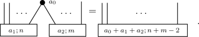  (4.5)

• 3. Removing a bubble:

  

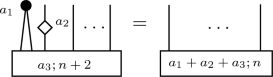  (4.6)

• 4. Moving $\zeta _a$:

  

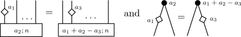  (4.7)

Furthermore we will assume the following:

• (L) The limit $\lim _{a\rightarrow 0}{D}_a$ exists.

We note that this assumption is quite natural, as it holds for all examples of the form given in Proposition 2.16. In this case, the limit is the sum of finite rank projections. Furthermore, from Lemma 2.21 Part 2 and Remark 2.17 we get the following lemma:

Lemma 4.2

A hermitian symmetric RFA is strongly separable and satisfies assumption (L).

The following lemma is a direct generalisation of [LP, Prop. 2.20].

Lemma 4.3

Let A be strongly separable symmetric RFA satisfying Assumption (L). Then $D_a\circ D_b=D_{a+b}$ for every $a,b\in {\mathbb {R}}_{>0}$ and the image of the idempotent $D_0:=\lim _{a\rightarrow 0}D_a$ is the centre Z(A) of A. It is an RFA with the restricted structure maps of A. Let us write

$$\begin{aligned} D_0=&\left[ A\xrightarrow {\pi _{A}}Z(A)\xrightarrow {\iota _{A}}A \right] ,&\left[ Z(A)\xrightarrow {\iota _{A}}A\xrightarrow {\pi _{A}}Z(A) \right] ={{\,\mathrm{id}\,}}_{Z(A)}, \end{aligned}$$

(4.8)

for the embedding and projection of Z(A).

In the rest of this section we define a symmetric monoidal functor ${\mathcal {Z}}_{A}:{{\mathcal {B}}ord_2^{area}}\rightarrow {{\mathcal {H}}ilb}$ using the RFA A. Let $S\in {{\mathcal {B}}ord_2^{area}}$. Then

$$\begin{aligned} {\mathcal {Z}}_{A}(S):=\bigotimes _{x\in \pi _0(S)}Z(A)^{(x)}, \end{aligned}$$

(4.9)

where $Z(A)^{(x)}=Z(A)$ and the superscript is used to label the tensor factors.

In the remainder of this section we give the definition of ${\mathcal {Z}}_{A}$ on morphisms. Let $(\Sigma ,{\mathcal {A}}):S\rightarrow T$ be a bordism with area and let us assume that $(\Sigma ,{\mathcal {A}})$ has no component with zero area. Choose a PLCW decomposition with area $\Sigma _k$, ${\mathcal {A}}_k$ for $k\in \left\{ 0,1,2 \right\}$ of the surface with area $(\Sigma ,{\mathcal {A}})$, such that the PLCW decomposition has exactly 1 edge on every boundary component. By this convention $\pi _0(S)\sqcup \pi _0(T)$ is in bijection with vertices on the boundary and with edges on the boundary.

Fig. 3

a Left and right sides (e, l) and (e, r) of an inner edge e, determined by the orientation of $\Sigma$ (paper orientation) and of e (arrow). b Convention for connecting tensor factors belonging to edge sides (e, l) and (e, r) of an inner edge e with the tensor factors belonging to the morphism $\beta _{{\mathcal {A}}_1(e)}^{(e)}$. c Conventions for the labels of the tensor factors for an ingoing boundary edge f with $(f,l)\in E$

Let us choose an edge for every face before glueing, which we call marked edge, and let us choose an orientation of every edge. For a face $f\in \Sigma _2$ which is an $n_f$-gon let us write (f, k), $k=1,\dots ,n_f$ for the sides of f, where (f, 1) denotes the marked edge of f, and the labeling proceeds counter-clockwise with respect to the orientation of f. We collect the sides of all faces into a set:

(4.10)

We double the set of edges by considering $\Sigma _1 \times \{l,r\}$, where “l” and “r” stand for left and right, respectively. Let $E \subset \Sigma _1 \times \{l,r\}$ be the subset of all (e, l) (resp. (e, r)), which have a face attached on the left (resp. right) side, cf. Fig. 3a. Thus for an inner edge $e\in \Sigma _1$ the set E contains both (e, l) and (e, r), but for a boundary edge $e'\in \Sigma _1$ the set E contains either $(e',l)$ or $(e',r)$. By construction of F and E we obtain a bijection

$$\begin{aligned} \Phi :F\xrightarrow {~\sim ~}E , \quad (f,k)\mapsto (e,x) , \end{aligned}$$

(4.11)

where e is the k’th edge on the boundary of the face f lying on the side x of e, counted counter-clockwise from the marked edge of f.

For every vertex $v\in \Sigma _0$ in the interior of $\Sigma$ or on an ingoing boundary component of $\Sigma$ choose a side of an edge $(e,x)\in E$ for which $v\in \partial (e)$. Let

$$\begin{aligned} V : \Sigma _0 {\setminus } \pi _0(T) \rightarrow E \end{aligned}$$

(4.12)

be the resulting function.

To define ${\mathcal {Z}}_{A}(\Sigma ,{\mathcal {A}})$ we proceed with the following steps.

• 1. Let us introduce the tensor products

  $$\begin{aligned} \begin{aligned} {\mathcal {O}}_{F}&:=\bigotimes _{(f,k) \in F}A^{(f,k)},&{\mathcal {O}}_{E}&:=\bigotimes _{(e,x) \in E}A^{(e,x)},\\ {\mathcal {O}}_{\mathrm {in}}&:=\bigotimes _{b\in \pi _0(S)}A^{(b,in)},&{\mathcal {O}}_{\mathrm {out}}&:=\bigotimes _{c\in \pi _0(T)}A^{(c,out)}. \end{aligned} \end{aligned}$$

  (4.13)

  Every tensor factor is equal to A, but the various superscripts will help us distinguish tensor factors in the source and target objects of the morphisms we define in the remaining steps.

• 2. Recall that by our conventions there is one edge in each boundary component and that we identified outgoing boundary edges with $\pi _0(T)$. Define the morphism

  $$\begin{aligned} {\mathcal {C}}:= \bigotimes _{e\in \Sigma _1{\setminus } \pi _0(T)} \beta _{{\mathcal {A}}_1(e)}^{(e)}: {\mathcal {O}}_{\mathrm {in}}\otimes {\mathcal {O}}_E\rightarrow {\mathcal {O}}_{\mathrm {out}}, \end{aligned}$$

  (4.14)

  where $\beta _{{\mathcal {A}}_1(e)}^{(e)}=\beta _{{\mathcal {A}}_1(e)}$, and where the tensor factors in ${\mathcal {O}}_{\mathrm {in}}\otimes {\mathcal {O}}_E$ are assigned to those of $\beta _{{\mathcal {A}}_1(e)}$ according to Fig. 3b, c.

• 3. Define the morphism

  $$\begin{aligned} {\mathcal {Y}}:=\prod _{v\in \Sigma _0{\setminus } \pi _0(T)} \zeta _{{\mathcal {A}}_0(v)}^{(V(v))} \in {\mathcal {B}}({\mathcal {O}}_E,{\mathcal {O}}_E), \end{aligned}$$

  (4.15)

  where

  $$\begin{aligned} \zeta _a^{(e,x)} = {{\,\mathrm{id}\,}}\otimes \cdots \otimes \zeta _a \otimes \cdots \otimes {{\,\mathrm{id}\,}}\in {\mathcal {B}}({\mathcal {O}}_E,{\mathcal {O}}_E) , \end{aligned}$$

  (4.16)

  where $\zeta _a$ maps the tensor factor $A^{(e,x)}$ to itself.

• 4. Assign to every face $f\in \Sigma _2$ obtained from an $n_f$-gon the morphism

  $$\begin{aligned} W_{{\mathcal {A}}_2(f)}^{f}=W_{{\mathcal {A}}_2(f)}^{(n_f)} : {\mathbb {C}}\rightarrow A_{(f,1)} \otimes \cdots \otimes A_{(f,n_f)} \end{aligned}$$

  (4.17)

  and take their tensor product:

  $$\begin{aligned} {\mathcal {F}}:=\bigotimes _{f\in \Sigma _2}\left( W_{{\mathcal {A}}_2(f)}^{f}\right) :{\mathbb {C}}\rightarrow {\mathcal {O}}_{F} . \end{aligned}$$

  (4.18)

• 5. We will now put the above morphisms together to obtain a morphism ${\mathcal {L}} : {\mathcal {A}}_{\mathrm {in}} \rightarrow {\mathcal {A}}_{\mathrm {out}}$. Denote by $\Uppi _\Phi$ the permutation of tensor factors induced by $\Phi :F\rightarrow E$,

  $$\begin{aligned} \Uppi _\Phi :{\mathcal {O}}_F\rightarrow {\mathcal {O}}_E . \end{aligned}$$

  (4.19)

  Using this, we define

  $$\begin{aligned} {\mathcal {K}}&:=\left[ {\mathbb {C}}\xrightarrow {{\mathcal {F}}}{\mathcal {O}}_F\xrightarrow {\Uppi _\Phi }{\mathcal {O}}_E \xrightarrow {{\mathcal {Y}}} {\mathcal {O}}_E\right] ,\end{aligned}$$

  (4.20)
  $$\begin{aligned} {\mathcal {L}}&:= \left[ {\mathcal {O}}_{\mathrm {in}}\xrightarrow {{{\,\mathrm{id}\,}}_{{\mathcal {O}}_{\mathrm {in}}}\otimes {\mathcal {K}}} {\mathcal {O}}_{\mathrm {in}}\otimes {\mathcal {O}}_{E} \xrightarrow {{\mathcal {C}}} {\mathcal {O}}_{\mathrm {out}} \right] . \end{aligned}$$

  (4.21)

• 6. Using the embedding and projection maps $\iota _{A}$, $\pi _{A}$ from (4.8) we construct the morphisms:

  $$\begin{aligned} {\mathcal {E}}_{\mathrm {in}}&:= \bigotimes _{b\in \pi _0(S)}\iota _{A}^{(b)}:{\mathcal {Z}}_{A}(S)\rightarrow {\mathcal {O}}_{\mathrm {in}},&{\mathcal {E}}_{\mathrm {out}}&:=\bigotimes _{c\in \pi _0(T)}\pi _{A}^{(c)}:{\mathcal {O}}_{\mathrm {out}}\rightarrow {\mathcal {Z}}_{A}(T), \end{aligned}$$

  (4.22)

  where $\iota _{A}^{(b)}=\iota _{A}:Z(A)^{(b)}\rightarrow A^{(b)}$ and $\pi _{A}^{(b)}=\pi _{A}:A^{(b)}\rightarrow Z(A)^{(b)}$. We have all ingredients to define the action of ${\mathcal {Z}}_{A}$ on morphisms:

  $$\begin{aligned} {\mathcal {Z}}_{A}(\Sigma ,{\mathcal {A}})&:= \left[ {\mathcal {Z}}_{A}(S)\xrightarrow {{\mathcal {E}}_{\mathrm {in}}} {\mathcal {O}}_{\mathrm {in}}\xrightarrow {{\mathcal {L}}} {\mathcal {O}}_{\mathrm {out}}\xrightarrow {{\mathcal {E}}_{\mathrm {out}}} {\mathcal {Z}}_{A}(T)\right] . \end{aligned}$$

  (4.23)

Now that we defined ${\mathcal {Z}}_{A({\mathbb {D}})}$ on bordisms with strictly positive area, we turn to the general case. Let $(\Sigma ,{\mathcal {A}}):S\rightarrow T$ be a bordism with area and let $\Sigma _+:S_+\rightarrow {T}_+$ denote the connected component of $(\Sigma ,{\mathcal {A}})$ with strictly positive area. We have that in ${{\mathcal {B}}ord_2^{area}}$

$$\begin{aligned} (\Sigma ,{\mathcal {A}})=({\Sigma }_+,{\mathcal {A}}_+)\sqcup (\Sigma {\setminus }{\Sigma }_+,0), \end{aligned}$$

(4.24)

where ${\mathcal {A}}_+$ denotes the restriction of ${\mathcal {A}}$ to $\pi _0(\Sigma _+)$. The bordism with zero area $(\Sigma {\setminus }{\Sigma }_+,0)$ defines a permutation $\kappa :\pi _0(S{\setminus }{S}_+)\rightarrow \pi _0(T{\setminus }{T}_+)$. Let ${\mathcal {Z}}_{A}(\Sigma {\setminus }{\Sigma }_+,0):{\mathcal {Z}}_{A}(S{\setminus }{S_+})\rightarrow {\mathcal {Z}}_{A}(T{\setminus }{T_+})$ be the induced permutation of tensor factors. We define

$$\begin{aligned} {\mathcal {Z}}_{A}(\Sigma ,{\mathcal {A}}):={\mathcal {Z}}_{A}(\Sigma {\setminus }{\Sigma }_+,0)\otimes {\mathcal {Z}}_{A}({\Sigma }_+,{\mathcal {A}}_+), \end{aligned}$$

(4.25)

where ${\mathcal {Z}}_{A}({\Sigma }_+,{\mathcal {A}}_+)$ is defined in (4.23).

Theorem 4.4

Let A be a strongly separable symmetric RFA satisfying Assumption (L).

• 1. The morphism defined in (4.23) is independent of the choice of the PLCW decomposition with area, the choice of marked edges of faces, the choice of orientation of edges and the assignment V.

• 2. The state sum construction yields an aQFT ${\mathcal {Z}}_{A}:{{\mathcal {B}}ord_2^{area}}\rightarrow {{\mathcal {H}}ilb}$ whose action on objects and morphisms is given by (4.9) and (4.25), respectively.

• 3. The commutative RFA corresponding to the aQFT ${\mathcal {Z}}_{A}$ is the center of A.

Proof

Part 1:

In order to show independence of the PLCW decomposition with area first notice that all conditions on A depend on the sum of the parameters. This implies that the construction is independent of the distribution of area, i.e. the maps ${\mathcal {A}}_k$ ($k\in \{0,1,2\}$). Checking that the construction is independent of the details of the PLCW decomposition can be done as in the case of TFTs (see e.g. [DKR, Lem. 3.5]), which is due to Conditions 1-4.

Part 2:

For an in-out cylinder with a single component with area a the morphism ${\mathcal {L}}$ in from (4.21) is exactly $D_a$ from (4.3). Clearly this is continuous in the parameter. When considering an in-out cylinder with several components, the zero area limit of the assigned morphism exists by Assumption (L) and it is clearly a permutation of tensor factors.

Functoriality follows from the fact that the morphisms $D_a$ form a semigroup (Lemma 4.3). Monoidality and symmetry directly follow from the construction, continuity in the area follows from Lemma 3.3, hence ${\mathcal {Z}}_A$ is indeed an aQFT.

Part 3: This directly follows from Lemma 4.3 and from the (4.9). $\square$

5 Example: 2d Yang–Mills Theory

The state sum construction of 2d Yang–Mills theory has been introduced by [Mig], was further developed for $G=U(N)$ in [Rus], and has been summarised in [Wit]; for a review see [CMR]. There, partition functions and expectation values of Wilson loops were calculated. These references also discuss the relation between the state-sum construction and the Lagrangian-based field theoretic approach to 2d Yang–Mills theory.

The proof of convergence of the (Boltzmann) plaquette weights has been shown in a different setting in [App]. In this section we will heavily rely on the representation theory of compact Lie groups, a standard reference is e.g. [Kna].

5.1 Two RFAs from a compact group G

Let G be a compact semisimple Lie group and $\int \,dx$ the Haar integral on G with the normalisation $\int _{G}1\,dx=1$. We denote with $L^2(G)$ the Hilbert space of square integrable complex functions on G, where the scalar product of $f,g\in L^2(G)$ is given by $\langle f,g\rangle :=\int f(x)^*g(x)dx$.

Let ${\hat{G}}$ denote a set of representatives of isomorphism classes of finite-dimensional simple unitary G-modules. Then for $V\in {\hat{G}}$ with inner product $\langle -,-\rangle _V$ and an orthonormal basis $\{e_i^V\}_{i=1}^{\dim (V)}$ let

$$\begin{aligned} \begin{aligned} f_{ij}^V:G&\rightarrow {\mathbb {C}}\\ g&\mapsto (\dim (V))^{1/2}\langle e_i^V,g.e_j^V\rangle _V \end{aligned} \end{aligned}$$

(5.1)

denote a matrix element function and let $M_V$ denote the linear span of these. The matrix element functions are orthonormal [Kna, Cor. 4.2]: for $V,W\in {\hat{G}}$, $i,j\in \left\{ 1,\dots ,\dim (V) \right\}$ and $k,l\in \left\{ 1,\dots ,\dim (W) \right\}$

$$\begin{aligned} \langle f_{ij}^V, f_{kl}^W \rangle =\delta _{ik}\delta _{jl}\delta _{V,W} \end{aligned}$$

(5.2)

where $\delta _{V,W}=1$ if $V=W$ and 0 otherwise. The character of V is defined as

$$\begin{aligned} \chi _V=(\dim (V))^{-1/2}\sum _{i=1}^{\dim (V)}f_{ii}^V. \end{aligned}$$

(5.3)

The Peter-Weyl theorem provides a complete orthonormal basis of $L^2(G)$ in terms of matrix element functions and of the square integrable class functions $Cl^2(G)$ in terms of characters:

$$\begin{aligned} L^2(G)\cong \bigoplus _{V\in {\hat{G}}}M_V\quad \text {and}\quad Cl^2(G)\cong \bigoplus _{V\in {\hat{G}}}{\mathbb {C}}.\chi _V \end{aligned}$$

(5.4)

as Hilbert space direct sums. Note that $L^2(G)\otimes L^2(G)\cong L^2(G\times G)$ and $Cl^2(G)\otimes Cl^2(G)\cong Cl^2(G\times G)$ isometrically by mapping $f \otimes f'$ to the function $(g,g') \mapsto f(g)f'(g')$. We will often use these isomorphisms without further notice.

In the following we will define a $\dagger$-RFA structure on $L^2(G)$ and $Cl^2(G)$. Let us start with defining the operator

$$\begin{aligned} \begin{aligned} \Delta :L^2(G)&\rightarrow L^2(G)\otimes L^2(G)\\ f&\mapsto \Delta (f)=\left[ (x,y)\mapsto f(xy) \right] , \end{aligned} \end{aligned}$$

(5.5)

which has norm 1. Let $\mu :=\Delta ^{\dagger }:L^2(G)\otimes L^2(G)\rightarrow L^2(G)$ be its adjoint, which is given by the convolution product. For $F\in L^2(G)\otimes L^2(G)$

$$\begin{aligned} \begin{aligned} \mu (F)(y)=\int _G F(x,x^{-1}y)\,dx. \end{aligned} \end{aligned}$$

(5.6)

Let $V\in {\hat{G}}$ and let us denote with $\sigma _V\in {\mathbb {R}}$ the value of the Casimir operator of G in the module V. We define the unit to be the heat kernel on G:

$$\begin{aligned} \begin{aligned} \eta _a:{\mathbb {C}}&\rightarrow L^2(G)\\ 1&\mapsto \eta _a(1)=\sum _{V\in {\hat{G}}}e^{-a\sigma _V}\dim (V)\chi _V \end{aligned} \end{aligned}$$

(5.7)

for $a\in {\mathbb {R}}_{>0}$.

Lemma 5.1

The sum in (5.7) is absolutely convergent for every $a\in {\mathbb {R}}_{>0}$.

Proof

This follows from [App, Sec. 3], which we explain now. Let us fix a maximal torus of G and let T denote its Lie algebra, let $\Lambda ^{+}\subset T^*$ denote the set of dominant weights and let $(-,-)$ be the inner product on $T^*$ induced by the Killing form and $|-|$ the induced norm. We will use that, since G is semisimple, there is a bijection of sets [Kna, Thm. 5.5]

(5.8)

From [Sug, (1.17)] and [App, (3.2)] we have that (by the Weyl dimension formula) for $V\in {\hat{G}}$ with dominant weight $\lambda _V\in \Lambda ^{+}$

$$\begin{aligned} \dim (V)\le N |\lambda _V|^m, \end{aligned}$$

(5.9)

where $N\in {\mathbb {R}}_{>0}$ is a constant independent of V and $2m=\dim (G)-{{\,\mathrm{rank}\,}}(G)$.

From [Sug, Lem. 1.1] we can express the value of the Casimir element in V using the highest weight $\lambda _V$ of V and the half sum of simple roots $\rho$ as

$$\begin{aligned} \sigma _V=(\lambda _V,\lambda _V+2\rho ). \end{aligned}$$

(5.10)

It follows directly [App, (3.5)] that

$$\begin{aligned} |\lambda _V|^2\le \sigma _V. \end{aligned}$$

(5.11)

We can give an estimate for the norm of $\lambda _V$ as follows. The choice of simple roots gives a bijection ${\mathbb {Z}}^{{{\,\mathrm{rank}\,}}(G)}\rightarrow \Lambda ^{+}$ which we write as $n\mapsto \lambda (n)$. Using the proof of [Sug, Lem. 1.3] there are $C_1,C_2\in {\mathbb {R}}_{\ge 0}$ such that for every $n\in {\mathbb {Z}}^{{{\,\mathrm{rank}\,}}(G)}$

$$\begin{aligned} C_1 \left\| {n}\right\| \le |\lambda (n)|\le C_2 \left\| {n}\right\| , \end{aligned}$$

(5.12)

where $\left\| {n}\right\| ^2=\sum _{i=1}^{{{\,\mathrm{rank}\,}}(G)}n_i^2$.

Let b(j) denote the number of $n\in {\mathbb {Z}}^{{{\,\mathrm{rank}\,}}(G)}$ with $\left\| {n}\right\| ^2=j$. We can easily give a (very rough) estimate of this by the volume of the ${{\,\mathrm{rank}\,}}(G)$-dimensional cube with edge length $2j^{1/2}+1$:

$$\begin{aligned} b(j)\le (2j^{1/2}+1)^{{{\,\mathrm{rank}\,}}(G)}. \end{aligned}$$

(5.13)

We compute the squared norm of $\eta _a$ following the computation in [App, Ex. 3.4.1].

$$\begin{aligned} \begin{aligned} \left\| {\eta _a}\right\| ^2&=\sum _{V\in {\hat{G}}}(\dim (V))^2 e^{-2a\sigma _V} {\mathop {=}\limits ^{(5.8)}} \sum _{\lambda \in \Lambda ^{+}}(\dim (V_{\lambda }))^2 e^{-2a\sigma _{V_{\lambda }}}\\ {\mathop {\le }\limits ^{(5.9)}}&N^2\sum _{\lambda \in \Lambda ^{+}}|\lambda |^{2m} e^{-2a\sigma _{V_{\lambda }}} {\mathop {\le }\limits ^{(5.11)}} N^2\sum _{\lambda \in \Lambda ^{+}}|\lambda |^{2m} e^{-2a|\lambda |^2}\\ {\mathop {\le }\limits ^{(5.12)}}&N^2C_2^{2m}\sum _{n\in {\mathbb {Z}}^{{{\,\mathrm{rank}\,}}(G)}} \left\| {n}\right\| ^{2m} e^{-2aC_1 \left\| {n}\right\| ^2} =N^2C_2^{2m}\sum _{j=1}^{\infty } b(j)j^m e^{-2aC_1j}\\ {\mathop {\le }\limits ^{(5.13)}}&N^2C_2^{2m}\sum _{j=1}^{\infty } (2j^{1/2}+1)^{{{\,\mathrm{rank}\,}}(G)}j^m e^{-2aC_1j}, \end{aligned} \end{aligned}$$

(5.14)

which converges. $\square$

Finally we define the counit as $\varepsilon _a:=\eta _a^{\dagger }:L^2(G)\rightarrow {\mathbb {C}}$. Explicitly, for $f\in L^2(G)$,

$$\begin{aligned} \varepsilon _a(f)=\langle \eta _a,f\rangle =\sum _{V\in {\hat{G}}}e^{-a\sigma _V}\dim (V)\int _G \chi _V(x) f(x^{-1})\,dx. \end{aligned}$$

(5.15)

Again for $a\in {\mathbb {R}}_{>0}$ let

$$\begin{aligned} \begin{aligned} P_a:L^2(G)&\rightarrow L^2(G)\\ f&\mapsto \mu (\eta _a\otimes f), \end{aligned} \end{aligned}$$

(5.16)

$\mu _a:=P_a\circ \mu$ and $\Delta _a:=\Delta \circ P_a$.

Proposition 5.2

$L^2(G)$, together with the family of morphisms $\mu _a$, $\eta _a$, $\Delta _a$ and $\varepsilon _a$ for $a\in {\mathbb {R}}_{>0}$ defined above is a strongly separable symmetric $\dagger$-RFA.

Before proving this proposition let us state a lemma. Let $V\in {\hat{G}}$ and define

$$\begin{aligned} \begin{aligned} \mu _a^{V}&:=\mu _a|_{M_V\otimes M_V},&\eta _a^V&:= e^{-a\sigma _V}\dim (V) \chi _V,\\ \Delta _{a}^{V}&:=\Delta |_{M_V},&\varepsilon _a^V&:=\varepsilon _a|_{M_V}. \end{aligned} \end{aligned}$$

(5.17)

From a computation using orthogonality of the $f_{ij}^V$ we can obtain the following formulas:

$$\begin{aligned} P_a(f_{ij}^V)&=e^{-a\sigma _V}f_{ij}^V\in M_V, \end{aligned}$$

(5.18)

$$\begin{aligned} \mu _a(f_{ij}^V\otimes f_{kl}^V)&=\delta _{jk} e^{-a\sigma _V} (\dim (V))^{-1/2}f_{il}^V\in M_V, \end{aligned}$$

(5.19)

$$\begin{aligned} \Delta _a(f_{ij}^V)&= e^{-a\sigma _V} (\dim (V))^{-1/2}\sum _{k=1}^{\dim (V)}f_{ik}^V \otimes f_{kj}^V\in M_V\otimes M_V, \end{aligned}$$

(5.20)

$$\begin{aligned} \varepsilon _a(f_{ij}^V)&= e^{-a\sigma _V} (\dim (V))^{1/2}\delta _{ij}. \end{aligned}$$

(5.21)

Lemma 5.3

Let $V\in {\hat{G}}$. Then $M_V$ is a strongly separable symmetric $\dagger$-RFA with the structure maps in (5.17).

Proof

Checking the algebraic relations is a straightforward calculation. As an example, we compute the window element of $M_V$.

$$\begin{aligned} \begin{aligned} \mu _{a_1}^V\circ \Delta _{a_2}^V\circ \eta _{a_3}^V&= \sum _{l=1}^{\dim (V)}\mu _{a_1}^V\circ \Delta _{a_2}^V(f_{ll}^V)e^{-a_3 \sigma _V} (\dim (V))^{1/2}\\&=\sum _{k,l=1}^{\dim (V)}\mu _{a_1}^V (f_{lk}^V\otimes f_{kl}^V)e^{-(a_2+a_3) \sigma _V}\\&= \sum _{k,l=1}^{\dim (V)}f_{ll}^V e^{-(a_1+a_2+a_3) \sigma _V}(\dim (V))^{-1/2}\\&=e^{-(a_1+a_2+a_3) \sigma _V} \dim (V) \chi _V= \eta _{a_1+a_2+a_3}^V, \end{aligned} \end{aligned}$$

(5.22)

which is clearly invertible. $\square$

Via the correspondence in Corollary 2.15, the finite dimensional RFA $M_V$ is given by the Frobenius algebra $M_V$ (with structure maps at $a=0$) and the element in the center $\sigma _V\cdot {{\,\mathrm{id}\,}}_{M_V}$.

Proof of Proposition 5.2

Let $V\in {\hat{G}}$ and let us compute the following norms.

$$\begin{aligned} \begin{aligned} \left\| {\eta _a^V}\right\| ^2&=e^{-2a\sigma _V}(\dim (V))^2\langle \chi _V,\chi _V\rangle = e^{-2a\sigma _V}\dim (V) \sum _{k,l=1}^{\dim (V)}\langle f_{kk}^{V},f_{ll}^{V}\rangle \\&= e^{-2a\sigma _V}(\dim (V))^2. \end{aligned} \end{aligned}$$

(5.23)

Let $\varphi =\sum _{i,j=1}^{\dim (V)}\varphi _{ij}f_{ij}^V\in M_V$ and compute

$$\begin{aligned} \begin{aligned} \left\| {\Delta _a^V(\varphi )}\right\| ^2=e^{-2a\sigma _V}(\dim (V))^{-1}\sum _{i,j,k=1}^{\dim (V)} |\varphi _{ij}|^2 \left\| {f_{ik}^V\otimes f_{kj}^V}\right\| ^2=e^{-2a\sigma _V} \left\| {\varphi }\right\| ^2, \end{aligned} \end{aligned}$$

(5.24)

so $\left\| {\Delta _a^V}\right\| =e^{-a\sigma _V}$. Since $M_V$ is a $\dagger$-RFA, $\left\| {\varepsilon _a^V}\right\| = \left\| {\eta _a^V}\right\|$ and $\left\| {\mu _a^V}\right\| = \left\| {\Delta _a^V}\right\|$.

We now would like to take the direct sum of the RFAs $M_V$ for all $V\in {\hat{G}}$, so we check the conditions of Proposition 2.16: the sum is convergent since it is the squared norm of $\eta _a\in L^2(G)$ and the supremum is clearly bounded. Therefore $L^2(G)$ is an RFA.

Clearly, $L^2(G)$ is strongly separable, symmetric and Hermitian by Lemma 5.3. $\square$

Now we turn to define an RFA structure on $Cl^2(G)$.

Proposition 5.4

The centre of $L^2(G)$ is $Cl^2(G)$ and it is a commutative $\dagger$-RFA.

Proof

Let us compute the morphism $D_a$ from (4.3). For $\varphi =\sum _{V\in {\hat{G}}}\sum _{i,j=1}^{\dim (V)}\varphi _{ij}^V f_{ij}^V\in L^2(G)$ we find:

$$\begin{aligned} \begin{aligned} D_a(\varphi )&=\mu _{a_2}\circ \sigma _{L^2(G),L^2(G)}\circ \Delta _{a_1}(\varphi )\\&=\mu _{a_2}\circ \sigma _{L^2(G),L^2(G)} \left( \sum _{V\in {\hat{G}}}\sum _{i,j,k=1}^{\dim (V)}\varphi _{ij}^V f_{ik}^V\otimes f_{kj}^V \right) e^{-a_1\sigma _V}(\dim (V))^{-1/2}\\&=\sum _{V\in {\hat{G}}}\sum _{i,j,k=1}^{\dim (V)}\varphi _{ij}^V e^{-a\sigma _V}(\dim (V))^{-1} \delta _{ij}f_{kk}^V\\&=\sum _{V\in {\hat{G}}}\sum _{i=1}^{\dim (V)}\varphi _{ii}^V e^{-a\sigma _V} (\dim (V))^{-1/2}\chi _V. \end{aligned} \end{aligned}$$

(5.25)

From this equation we immediately have that $D_a|_{Cl^2(G)}=P_a|_{Cl^2(G)}$. We now show that $D_a|_{(Cl^2(G))^{\perp }}=0$. Using (5.4), we have that $\varphi \in (Cl^2(G))^{\perp }\subset L^2(G)$ if and only if for every $W\in {\hat{G}}$ $\langle \chi _W,\varphi \rangle =0$. We can compute this using the orthogonality relation (5.2) to get the following: $\varphi \in (Cl^2(G))^{\perp }$ if and only if for every $W\in {\hat{G}}$ we have that $\sum _{k=1}^{\dim (W)}\varphi ^W_{kk}=0$. By (5.25) we get that $D_a(\varphi )=0$.

We have shown that the image of $D_0$ is $Cl^2(G)$, therefore it is the centre of $L^2(G)$ by Lemma 4.3. Furthermore it is a $\dagger$-RFA, since $L^2(G)$ is a $\dagger$-RFA and $D_0$ is self-adjoint. $\square$

For completeness we give the comultiplication $\Delta _a^{Cl^2(G)}$ of $Cl^2(G)$. For $\varphi =\sum _{V\in {\hat{G}}}\varphi ^V \chi _V\in Cl^2(G)$

$$\begin{aligned} \Delta _a^{Cl^2(G)}(\varphi )=\sum _{V\in {\hat{G}}}\varphi ^V e^{-a\sigma _V} (\dim (V))^{-2}\chi _V\otimes \chi _V. \end{aligned}$$

(5.26)

Remark 5.5

Note that for both $L^2(G)$ and $Cl^2(G)$, the $a\rightarrow 0$ limit of the multiplication and comultiplication exists (by definition), but the $a\rightarrow 0$ limit of the unit and counit does not, cf. the proof of Proposition 5.2.

5.2 State sum construction of 2d Yang–Mills theory

In this section we give state sum data for 2d YM theory following [Wit]. The plaquette weights $W_a^k:{\mathbb {C}}\rightarrow (L^2(G))^{\otimes k}$ for $k\in {\mathbb {Z}}_{\ge 0}$ and $a\in {\mathbb {R}}>0$ are

$$\begin{aligned} W_a^{k}(1)(x_1,\dots ,x_k)=\sum _{V\in {\hat{G}}}e^{-a\sigma _V} \dim (V) \chi _V(x_1\cdots x_k) , \end{aligned}$$

(5.27)

and the contraction and $\zeta _a$ are given by

$$\begin{aligned} \beta _a:=\left( W_a^{2}\right) ^{\dagger },\quad \zeta _a:= P_a, \end{aligned}$$

(5.28)

where $P_a$ is as in (5.16). Now we are ready to define 2d YM theory, which maps ${\mathbb {S}}^1$ to the centre of $L^2(G)$, see Proposition 5.4.

Definition 5.6

The 2-dimensional Yang–Mills (2d YM) theory with gauge group G is the state sum area-dependent QFT

$$\begin{aligned} \begin{aligned} {\mathcal {Z}}_{\mathrm {YM}}^{G}:={\mathcal {Z}}_{L^2(G)}:{{\mathcal {B}}ord_2^{area}}&\rightarrow {{\mathcal {H}}ilb}\end{aligned} \end{aligned}$$

(5.29)

of Theorem 4.4. The commutative RFA it assigns to the circle is ${\mathcal {Z}}_{\mathrm {YM}}^{G}({\mathbb {S}}^1)= Cl^2(G)$.

Next we compute ${\mathcal {Z}}_{\mathrm {YM}}^{G}$ on connected surfaces with area and $b\ge 0$ boundary components. For $b=0$ the result agrees with [Wit, Eqn. (2.51)] (see also [Rus, Eqn. (27)]).

Proposition 5.7

Let $(\Sigma ,a):({\mathbb {S}}^1)^{\sqcup b_{\mathrm {in}}}\rightarrow ({\mathbb {S}}^1)^{\sqcup b_{\mathrm {out}}}$ be a connected bordism of genus g with $b_{\mathrm {in}}$ ingoing and $b_{\mathrm {out}}$ outgoing boundary components and with area a. Then for $V_j\in {\hat{G}}$ for $j=1,\dots ,b_{\mathrm {out}}$ we have

$$\begin{aligned} \begin{aligned}&{\mathcal {Z}}_{\mathrm {YM}}^{G}\left( \Sigma _ ,a \right) (\chi _{V_1}\otimes \dots \otimes \chi _{V_{b_{\mathrm {in}}}})\\&\quad = {\left\{ \begin{array}{ll} \sum _{V\in {\hat{G}}}e^{-a\sigma _V} (\dim (V))^{\chi ( \Sigma )}\cdot (\chi _V)^{\otimes b_{\mathrm {out}}} &{}\text {if}\; b_{\mathrm {in}}=0\\ e^{-a\sigma _{V_1}}(\dim (V_1))^{\chi ( \Sigma )}\cdot (\chi _{V_1})^{\otimes b_{\mathrm {out}}} &{}\text {if}\; b_{\mathrm {in}}\ge 1 \,\text {and}\, V_1=\dots = V_{b_{\mathrm {in}}}\\ 0&{}\text {else} \end{array}\right. } , \end{aligned} \end{aligned}$$

(5.30)

where $\chi ( \Sigma )=2-2g-b_{\mathrm {in}}-b_{\mathrm {out}}$ is the Euler characteristic of $\Sigma$. For $b_{\mathrm {in}}=0$ ($b_{\mathrm {out}}=0$) the source (the target) is ${\mathbb {C}}$ and the factors of $\chi _V$ or $\chi _{V_j}$ are absent.

Proof

We first consider the case that $b:=b_{\mathrm {out}} \ge 1$ and $b_{\mathrm {in}}=0$. Denote the map assigned to the two-holed torus by $\varphi _a=\mu \circ \left( {{\,\mathrm{id}\,}}\otimes (\mu \circ \sigma _{L^2(G),L^2(G)}\circ \Delta \right) \circ \Delta _a^{(2)}:L^2(G)\rightarrow L^2(G)$ and compute

$$\begin{aligned} \begin{aligned} \varphi _a(f_{ij}^V)&=\mu \circ \left( {{\,\mathrm{id}\,}}\otimes (\mu \circ \sigma _{L^2(G),L^2(G)} \right) \left( \sum _{k,l=1}^{\dim (V)}e^{-a\sigma _V}(\dim (V))^{-1} f_{ik}^{V}\otimes f_{kl}^{V} \otimes f_{lj}^{V}\right) \\&=\sum _{k,l=1}^{\dim (V)}e^{-a\sigma _V}(\dim (V))^{-2} \delta _{jk}\delta _{kl}f_{il}^V =e^{-a\sigma _V}(\dim (V))^{-2}f_{ij}^V . \end{aligned} \end{aligned}$$

(5.31)

Using this, we compute for $a_0,\dots ,a_{g+1}\in {\mathbb {R}}_{>0}$ with $a=\sum _{i=0}^{g+1}a_i$ that

$$\begin{aligned} \begin{aligned} \Delta _{a_{g+1}}^{(b)} \circ \prod _{i=1}^{g}\varphi _{a_i}\circ \eta _{a_0}&=\Delta _{a_{g+1}}^{(b)} \left( \sum _{V\in {\hat{G}}} e^{-(a-a_{g+1})\sigma _V} (\dim (V))^{1-2g}\chi _V \right) \\&=\left[ (x_1,\dots ,x_b)\!\mapsto \!\!\left( \sum _{V\in {\hat{G}}}e^{-a\sigma _V} (\dim (V))^{1-2g}\chi _V(x_1\dots x_b)\right) \right] . \end{aligned} \end{aligned}$$

(5.32)

Finally, we need to compose (5.32) with $\pi ^{\otimes b}$ to get (5.30), where $\pi :L^2(G)\rightarrow Cl^2(G)$ is the projection onto the image of $D_0$. We compute using (5.25):

$$\begin{aligned} \begin{aligned} \pi ^{\otimes b}(\chi _V(x_1\dots x_b))&= \pi ^{\otimes b}\left( \sum _{k_1,\dots ,k_b=1}^{\dim (V)}(\dim (V))^{-b/2} f_{k_1 k_2}^{V}(x_1)\dots f_{k_b k_1}^{V}(x_b)\right) \\&=(\dim (V))^{1-b} \chi _V(x_1)\dots \chi _V(x_b). \end{aligned} \end{aligned}$$

(5.33)

For the case $b_{\mathrm {in}}=b_{\mathrm {out}}=0$ we use functoriality. Let $\Sigma '$ the surface obtained by cutting out a disk from $\Sigma$. Compose ${\mathcal {Z}}_{\mathrm {YM}}^{G}\left( \Sigma ' ,a-a' \right)$ with $\varepsilon _{a'}$ and use (5.21).

For the case $b_{\mathrm {in}}\ne 0$ we need to turn back outgoing boundary components by composing with cylinders with two ingoing boundary components and with area a, which we denote with (C, a). For $U,W\in {\hat{G}}$ we have

$$\begin{aligned} {\mathcal {Z}}_{\mathrm {YM}}^{G}(C,a)(\chi _{U},\chi _W)=e^{-a\sigma _U}\delta _{U,V}. \end{aligned}$$

(5.34)

Using the result for the $b_{\mathrm {in}}=0$ case and (5.34) we get the claimed expression. $\square$

Remark 5.8

As already noted in Remark 5.5, $\eta _a$ and $\varepsilon _a|_{Cl^2(G)}$, i.e. the value of ${\mathcal {Z}}_{\mathrm {YM}}^{G}$ on a disc with one outgoing (resp. one ingoing) boundary component, do not have zero area limits. On the other hand, the expression (5.30) has a zero area limit if $\chi (\Sigma )=2-2g-(b_{\mathrm {in}}+b_{\mathrm {out}}) <0$. Note that this is the condition of $\Sigma$ being stable. Indeed, the $\chi _V$ are orthogonal for different V and have norm $\left\| {\chi _V}\right\| =1$, and for a given $\alpha \in {\mathbb {Z}}$ the sum $\sum _{V\in {\hat{G}}} (\dim (V))^{\alpha }$ converges if $\alpha \le -2$. To see this, use the bijection from (5.8) and the estimate from (5.9) to get

$$\begin{aligned} \sum _{V\in {\hat{G}}} (\dim (V))^{\alpha }\le \sum _{\lambda \in \Lambda ^+}(\dim (V_{\lambda }))^{\alpha }\le N\sum _{\lambda \in \Lambda ^+}|\lambda |^{m\alpha }, \end{aligned}$$

(5.35)

which converges for $-m\alpha >{{\,\mathrm{rank}\,}}(G)$ by [Sug, Lem. 1.3]. Then use that $m=(\dim (G)-{{\,\mathrm{rank}\,}}(G))/2$ and that $3{{\,\mathrm{rank}\,}}(G)\le \dim (G)$ to get $\alpha <-1$, and since $\alpha$ is an integer $\alpha \le -2$. These limits are related in [Wit] to volumes of moduli spaces of flat connections (see e.g. [KMT] for more results and references). For example for $G = SU(2)$ we have, for $g \ge 2$ and $b_{\mathrm {in}}=b_{\mathrm {out}}=0$,

$$\begin{aligned} \lim _{a \rightarrow 0} {\mathcal {Z}}_{\mathrm {YM}}^{SU(2)}\left( \Sigma ,a \right) (1) = \sum _{n=1}^\infty n^{-2g+2} = \zeta (2g-2) , \end{aligned}$$

(5.36)

where $\zeta$ is the Riemann zeta-function. For general G, these functions are also referred to as Witten zeta-functions, see e.g. [KMT].

A Proof of Joint Continuity

The following lemma will be instrumental in showing that various joint continuity conditions hold automatically in ${{\mathcal {H}}ilb}$. A similar statement can be found in [KMD, Sec. 2].

Lemma A.1

Let ${\mathcal {H}}_i\in {{\mathcal {H}}ilb}$ ($i=1,2$). Let X be a subset of a finite-dimensional normed vector space (e.g. $X = {\mathbb {R}}_{\ge 0}$). Equip X with the induced topology and let $a\mapsto S^{(i)}_a$ be two continuous maps $X\rightarrow {\mathcal {B}}({\mathcal {H}}_i)$. Then the map $X^2\rightarrow {\mathcal {B}}({\mathcal {H}}_1\otimes {\mathcal {H}}_2)$, $(a,b)\mapsto S^{(1)}_a\otimes S^{(2)}_b$ is jointly continuous.

Proof

We will first show that the map $a\mapsto \left\| {S^{(i)}_a}\right\|$ is bounded on compact subsets of X. Let $K\subset X$ be compact. By strong continuity we have that for every $h\in {\mathcal {H}}_i$ the map $a\mapsto S^{(i)}_a(h)$ is continuous, so in particular the map $a\mapsto \left\| {S^{(i)}_a(h)}\right\|$ is continuous, hence bounded on K. By the Uniform Boundedness Principle [Con1, Ch. III.14] the map $a\mapsto \left\| {S^{(i)}_a}\right\|$ is bounded on K.

Now we turn to the claim in the lemma. Let $a_0,b_0\in X$ and $\kappa ,\varepsilon \in {\mathbb {R}}_{>0}$ be fixed. We will show that the map $(a,b)\mapsto S^{(1)}_a\otimes S^{(2)}_b$ is continuous at $(a_0,b_0)$.

For $T\in {\mathcal {H}}_1\otimes {\mathcal {H}}_2$ take a sequence $\left\{ T_n \right\} _{n}$ in the algebraic tensor product of ${\mathcal {H}}_1$ and ${\mathcal {H}}_2$ such that $T_n\xrightarrow {n\rightarrow \infty } T$. We have the estimate

$$\begin{aligned} \begin{aligned}&\left\| {(S^{(1)}_a\otimes S^{(2)}_b-S^{(1)}_{a_0}\otimes S^{(2)}_{b_0})T}\right\| \\&\quad \le \left\| {(S^{(1)}_a\otimes S^{(2)}_b-S^{(1)}_{a_0}\otimes S^{(2)}_{b_0})}\right\| \cdot \left\| {T-T_n}\right\| + \left\| {(S^{(1)}_a\otimes S^{(2)}_b-S^{(1)}_{a_0}\otimes S^{(2)}_{b_0})T_n}\right\| . \end{aligned} \end{aligned}$$

(A.1)

We give an estimate for the first term on the right hand side of (A.1). Fix some $\delta _1>0$. Then by the above boundedness result there is a $\kappa >0$ such that for every $a,b\in X$ with $|a-a_0|+|b-b_0|<\delta _1$ we have $\left\| {S^{(1)}_{a}}\right\| <\kappa$ and $\left\| {S^{(2)}_{b}}\right\| <\kappa$. So we have

$$\begin{aligned} \begin{aligned} \left\| {S^{(1)}_a\otimes S^{(2)}_b-S^{(1)}_{a_0}\otimes S^{(2)}_{b_0}}\right\|&\le \left\| {S^{(1)}_a}\right\| \cdot \left\| {S^{(2)}_b}\right\| + \left\| {S^{(1)}_{a_0}}\right\| \cdot \left\| {S^{(2)}_{b_0}}\right\| \\&\le \ \kappa ^2 + \left\| {S^{(1)}_{a_0}}\right\| \cdot \left\| {S^{(2)}_{b_0}}\right\| =:N_{a_0,b_0}^{\kappa }. \end{aligned} \end{aligned}$$

(A.2)

Since $T_n\xrightarrow {n\rightarrow \infty } T$, we can choose n (which we keep fixed from now on) such that

$$\begin{aligned} \left\| {T-T_n}\right\| <\frac{\varepsilon }{2N_{a_0,b_0}^{\kappa }}. \end{aligned}$$

(A.3)

Putting (A.2) and (A.3) together we get

$$\begin{aligned} \left\| {(S^{(1)}_a\otimes S^{(2)}_b-S^{(1)}_{a_0}\otimes S^{(2)}_{b_0})}\right\| \cdot \left\| {T-T_n}\right\| \le \frac{\varepsilon }{2}. \end{aligned}$$

(A.4)

We give an estimate for the last term in (A.1). Recall that each $T_n$ was chosen in the algebraic tensor product of ${\mathcal {H}}_1$ and ${\mathcal {H}}_2$. Thus $T_n$ is a finite sum of elementary tensors,

$$\begin{aligned} T_n=\sum _{j=1}^{t_n}x_n^j\otimes y_n^j \end{aligned}$$

(A.5)

for $t_n\in {\mathbb {Z}}_{\ge 1}$, $x_n^j\in {\mathcal {H}}^{(1)}$ and $y_n^j\in {\mathcal {H}}^{(2)}$. Using this, we get:

$$\begin{aligned} \begin{aligned}&\left\| {(S^{(1)}_a-S^{(1)}_{a_0})\otimes S^{(2)}_b T_n +S^{(1)}_{a_0}\otimes (S^{(2)}_b-S^{(2)}_{b_0})T_n}\right\| \\&\quad \le \sum _{j=1}^{t_n}\left( \left\| {(S^{(1)}_a-S^{(1)}_{a_0})x_n^j}\right\| \cdot \left\| {S^{(2)}_b}\right\| \cdot \left\| {y_n^j}\right\| + \left\| {(S^{(1)}_{a_0}}\right\| \cdot \left\| {x_n^j}\right\| \cdot \left\| {(S^{(2)}_b-S^{(2)}_{b_0})y_n^j}\right\| \right) . \end{aligned} \end{aligned}$$

(A.6)

By strong continuity of $a\mapsto S^{(i)}_a$ we can chose $\delta _2 >0$ such that for every $a,b\in X$ with $|a-a_0|+|b-b_0|<\delta _2$ we have

$$\begin{aligned} \left\| {(S^{(1)}_a-S^{(1)}_{a_0})x_n^j}\right\|<\frac{\varepsilon }{4t_n \kappa \left\| {y_n^j}\right\| } \quad \text { and }\quad \left\| {(S^{(2)}_b-S^{(2)}_{b_0})y_n^j}\right\| <\frac{\varepsilon }{4t_n \left\| {S^{(1)}_{a_0}}\right\| \cdot \left\| {x_n^j}\right\| }, \end{aligned}$$

(A.7)

for every $j=1,\dots ,t_n$, since these are only finitely many conditions to satisfy. Let $\delta :=\min \left\{ \delta _1,\delta _2 \right\}$. Then for every $a,b\in X$ with $|a-a_0|+|b-b_0|<\delta$ we have that

$$\begin{aligned} \begin{aligned} \left\| {(S^{(1)}_a\otimes S^{(2)}_b-S^{(1)}_{a_0}\otimes S^{(2)}_{b_0})T_n}\right\| \le \frac{\varepsilon }{2}. \end{aligned} \end{aligned}$$

(A.8)

Finally, using (A.4) and (A.8) we have that

$$\begin{aligned} \left\| {(S^{(1)}_a\otimes S^{(2)}_b-S^{(1)}_{a_0}\otimes S^{(2)}_{b_0})T}\right\| <\varepsilon . \end{aligned}$$

(A.9)

$\square$

Proof of Lemma 2.5

Let $\varphi _{a_1,\dots ,a_N} : A^{\otimes n} \rightarrow A^{\otimes m}$ be a morphism in ${{\mathcal {H}}ilb}$ tensor generated by $\mu _a$, $\eta _a$, $\Delta _a$ and $\varepsilon _a$, involving a total of N connected components when drawing it using the graphical calculus, with parameters $a_1,\dots ,a_N$. One can write $\varphi _{a_1,\dots ,a_N}$ in the form $\varphi ^{(1)}_{\varepsilon _1}\circ \left( \bigotimes _{i=1}^{N} P_{a_i-\varepsilon _1-\varepsilon _2} \right) \circ \varphi ^{(2)}_{\varepsilon _2}$ for some $\varepsilon _1,\varepsilon _2\in {\mathbb {R}}_{>0}$ and morphisms $\varphi ^{(1)}_{\varepsilon _1}$ and $\varphi ^{(2)}_{\varepsilon _2}$. Then by separate continuity of the composition of ${{\mathcal {H}}ilb}$ and joint continuity of $\bigotimes _{i=1}^{N}P_{a_i}$ by Lemma A.1 the morphism $\varphi _{a_1,\dots ,a_N}$ is jointly continuous in the parameters $a_1,\dots ,a_N$. $\square$

References

Abrams, L.: Two dimensional topological quantum field theories and Frobenius algebras. J. Knot Theor. Ramif. 5, 569–587 (1996)
Applebaum, D.: Infinitely divisible central probability measures on compact Lie groups—regularity, semigroups and transition kernels. Ann. Probab. 39(6), 2474–2496 (2011). arXiv:1006.4711 [math.PR]
Banyaga, A.: Formes-volume sur les variétés à bord. Enseignement Math. 2, 127–131 (1974)
Bartlett, B.H.: Categorical Aspects of Topological Quantum Field Theories. PhD thesis, Utrecht University (2005) arXiv:math/0512103 [math.QA]
Radjavi, H., Rosenthal, P.: Simultaneous Triangularization. Universitext. Springer-Verlag, New York (1994)
Bachas, C., Petropoulos, P.M.S.: Topological models on the lattice and a remark on string theory cloning. Commun. Math. Phys. 152, 191–202 (1993). arXiv:hep-th/9205031
Brunner, I.: Area preserving symmetry in two-dimensional quantum field theory. BONN-IB-95-36, diploma thesis (1995)
Carqueville, N.: Lecture notes on 2-dimensional defect TQFT. Banach Cent. Publ. 114, 49–84 (2018). arXiv:1607.05747 [math.QA]
Cordes, S., Moore, G., Ramgoolam, S.: Lectures on 2D Yang–Mills theory, equivariant cohomology and topological field theories. Nucl. Phys. Proc. Suppl. 41, 184–244 (1995). arXiv:hep-th/9411210
Conway, J.B.: A Course in Functional Analysis. Graduate Texts in Mathematics, vol. 96. Springer, Berlin (1994)
Conway, J.B.: A Course in Operator Theory. Graduate Studies in Mathematics, vol. 21. American Mathematical Society, Providence (2000)
Carqueville, N., Runkel, I.: Introductory lectures on topological quantum field theory. arXiv:1705.05734 [math.QA]
Cunha, B.G.C., Teotonio-Sobrinho, P.: Quasi-topological field theories in two dimensions as soluble models. Int. J. Mod. Phys. A 13, 3667–3690 (1998). arXiv:hep-th/9703014
Davydov, A.: Centre of an algebra. Adv. Math. 225(1), 319–348 (2010). arXiv:0908.1250 [math.CT]
Dijkgraaf, R.H.: A geometrical approach to two-dimensional conformal field theory. PhD thesis, Utrecht University (1989)
Davydov, A., Kong, L., Runkel, I.: Field theories with defects and the centre functor. In: Sati, H., Schreiber, U. (eds.) Mathematical Foundations of Quantum Field and Perturbative String Theory. AMS, Providence (2011). arXiv:1107.0495 [math.QA]
Engel, K.J., Nagel, R.: One-Parameter Semigroups for Linear Evolution Equations. Graduate Texts in Mathematics. Springer, New York (1999)
Fukuma, M., Hosono, S., Kawai, H.: Lattice topological field theory in two dimensions. Commun. Math. Phys. 161, 157–175 (1994). arXiv:hep-th/9212154
Kanzaki, T.: Special type of separable algebras over a commutative ring. Proc. Jpn. Acad. 40, 781–786 (1964)
Kirillov Jr., A.: On piecewise linear cell decompositions. Algebr. Geom. Topol. 12, 95–108 (2012). arXiv:1009.4227 [math.GT]
Khalil, R., Al-Mirbati, R., Drissi, D.: Tensor product semigroups. Eur. J. Pure Appl. Math. 3(5), 881–898 (2010)
Komori, Y., Matsumoto, K., Tsumura, H.: Zeta-functions of weight lattices of compact connected semisimple Lie groups. Siauliai Math. Semin. 18, 149–179 (2015). arXiv:1011.0323 [math.NT]
Knapp, A.W.: Lie Groups Beyond an Introduction. Progress in Mathematics. Birkhäuser, Boston (2002)
Kock, J.: Frobenius Algebras and 2D Topological Quantum Field Theories. Cambridge University Press, Cambridge (2004)
Kadison, R.V., Ringrose, J.R.: Fundamentals of the Theory of Operator Algebras: Elementary Theory, vol. I. Academic Press, New York (1983)
Kubrusly, C.S.: Elements of Operator Theory. Springer, Berlin (2001)
Lauda, A.D., Pfeiffer, H.: State sum construction of two-dimensional open-closed topological quantum field theories. J. Knot Theor. Ramif. 16, 1121–1163 (2007). arXiv:math/0602047 [math.QA]
Migdal, A.A.: Recursion equations in gauge field theories. Sov. Phys. JETP 42, 413 (1975)
Moser, J.: On the volume elements on a manifold. Trans. Am. Math. Soc. 120, 286–294 (1965)
Pierce, R.S.: Associative Algebras. Graduate Texts in Mathematics, vol. 88. Springer, Berlin (1982)
Runkel, I., Szegedy, L.: Topological field theory on r-spin surfaces and the Arf invariant. arXiv:1802.09978 [math.QA]
Rusakov, B.E.: Loop averages and partition functions in U(N) gauge theory on two-dimensional manifolds. Mod. Phys. Lett. A 5, 693 (1990)
Segal, G.: Topological Field Theory (‘Stanford Notes’). Lecture notes from ITP Workshop on Geometry and Physics (1999)
Selinger, P.: Dagger compact closed categories and completely positive maps. Electron. Notes Theor. Comput. Sci. 170, 139–163 (2007)
Sugiura, M.: Fourier series of smooth functions on compact Lie groups. Osaka J. Math. 8, 33–47 (1971)
Szegedy, L.: State-Sum Construction of Two-Dimensional Functorial Field Theories. PhD thesis, Universität Hamburg (2018). http://ediss.sub.uni-hamburg.de/volltexte/2018/9321/
Turaev, V.G.: Quantum Invariants of Knots and 3-Manifolds. de Gruyter, Berlin (1994)
Witten, E.: On quantum gauge theories in two dimensions. Commun. Math. Phys. 141, 153–209 (1991)
Acknowledgements
The authors thank Yuki Arano, Nils Carqueville, Alexei Davydov, Reiner Lauterbach, Pau Enrique Moliner, Chris Heunen, André Henriques, Ehud Meir, Catherine Meusburger, Gregor Schaumann, Richard Szabo and Stefan Wagner for helpful discussions and comments. We also thank the referees for their detailed comments which significantly improved the exposition of this paper. LS is supported by the DFG Research Training Group 1670 “Mathematics Inspired by String Theory and Quantum Field Theory”.
Funding
Open access funding provided by Institute of Science and Technology (IST Austria).
Author information
Authors and Affiliations
Corresponding author
Additional information
Communicated by Y. Kawahigashi.
Publisher's Note
Springer Nature remains neutral with regard to jurisdictional claims in published maps and institutional affiliations.