
Abstract
We classify all (locally) homogeneous Levi non-degenerate real hypersurfaces in \({{\mathbb {C}}}^3\) with symmetry algebra of dimension \(\ge 6\).
1 Introduction
The main goal of this paper is to provide the complete (local) classification of multiply-transitive Levi non-degenerate real hypersurfaces in \({{\mathbb {C}}}^3\), i.e. hypersurfaces with transitive symmetry algebra and stabilizer of dimension \(\ge 1\) (Theorem 1.1). It is known [6, 21] that any real hypersurface in \({{\mathbb {C}}}^n\) with non-degenerate Levi form has symmetry algebra of dimension at most \(n(n+2)\), which is achieved if and only if it is locally equivalent (under biholomorphic transformations) to a hyperquadric given by:
In \({{\mathbb {C}}}^3\), the next possible dimension of the symmetry algebra for a Levi non-degenerate hypersurface is 8, which is achieved for the so-called Winkelmann hypersurface [23]:
where \((z_1,z_2,w)\) are holomorphic coordinates in \({{\mathbb {C}}}^3\). The 8-dimensional symmetry algebra is transitive on this hypersurface. Moreover, it is also transitive on the two open (unbounded) domains in \({{\mathbb {C}}}^3\) separated by this hypersurface. We show in this paper (Theorem 1.3) that hyperquadrics and the Winkelmann hypersurface are the only homogeneous Levi non-degenerate hypersurfaces in \({{\mathbb {C}}}^3\) whose symmetry algebras have open orbits in \({{\mathbb {C}}}^3\).
The analogous classification result in \({{\mathbb {C}}}^2\) was obtained by Élie Cartan in his pioneering works [3, 4] on this subject. He also used this result to prove that the only bounded homogeneous domain in \({{\mathbb {C}}}^2\) is the interior of a hypersphere. He claimed to prove a similar result for bounded homogeneous domains in \({{\mathbb {C}}}^3\), but the details of this proof were never published and seem to be hidden in the archives of his notes.Footnote 1 This led him to believe [5] that the only bounded homogeneous domains in \({{\mathbb {C}}}^n\) for any \(n\ge 2\) are given by symmetric homogeneous spaces. However, this proved to be not correct, and the first counterexample was discovered by Piatetski-Shapiro in 1959 [16].
Levi non-degenerate hypersurfaces in \({{\mathbb {C}}}^3\) with large symmetry algebras were extensively studied in a series of papers by Loboda. He classified all Levi non-degenerate hypersurfaces with 7-dimensional symmetry algebra [11, 12], as well as all hypersurfaces with 6-dimensional symmetry algebra and positive definite Levi form [13]. In our paper, we complete the classification of all multiply-transitive hypersurfaces in \({{\mathbb {C}}}^3\) by providing the full list of Levi indefinite hypersurfaces in \({{\mathbb {C}}}^3\) with 6-dimensional symmetry algebra. We also correct the Levi definite list [13, Theorem 3] by adding one missing hypersurface with 6-dimensional symmetry algebra:
Here \(z_1 = x_1+iy_1\), \(z_2=x_2+iy_2\), \(w=u+iv\) so this hypersurface is tubular (see Sect. 4 for the definition). This corresponds to the Levi definite real form of case D.6-1 in [9]—see also Table 8. The symmetry algebra here is isomorphic to the semidirect product of \(\mathfrak {sl}(2,{{\mathbb {R}}})\) and the 3-dimensional Heisenberg algebra. In Table 9, we match Loboda’s classifications with our results.
The main idea of our classification approach is to pass from Levi non-degenerate hypersurfaces in \({{\mathbb {C}}}^n\) to their complex analogue, which turns out to be a complete system of 2nd order PDEs on one function of \(n-1\) independent variables (see Sect. 2). Such systems of PDEs have the same dimension for their symmetry algebra, which is multiply-transitive on the first jet-space \(J^1({{\mathbb {C}}}^{n-1},{{\mathbb {C}}})\) if and only if the corresponding real hypersurface in \({{\mathbb {C}}}^n\) is multiply-transitive.
This idea of passing from real hypersurfaces in \({{\mathbb {C}}}^n\) to families of complex hypersurfaces (also known as Segre varieties) was first introduced by Segre [17, 18], explored in more detail in the original work of Cartan [4] in the case of real hypersurfaces in \({{\mathbb {C}}}^2\), and was extended to more general cases in [1, 14, 19, 20, 22].
Geometrically, any Levi non-degenerate hypersurface \(M\subset {{\mathbb {C}}}^n\) inherits a natural CR structure of codimension 1, which consists of a contact distribution \(C\subset TM\) equipped with a complex structure \(J:C\rightarrow C\). This complex structure is compatible with the natural conformal symplectic form on C and is integrable. Both these conditions are equivalent to the fact that the eigenspaces J(i) and \(J(-i)\) of the operator J on the complexification \(C^{{{\mathbb {C}}}}\) should be integrable subdistributions of the complexified contact distribution.
The corresponding complete systems of second order PDEs are encoded as complex analytic manifolds of dimension \(2n-1\) equipped with contact distribution C decomposed into the direct sum of two completely integrable subdistributions E and V. Such structures are called integrable Legendrian contact (ILC) structures and they were studied in detail in [9]. The fundamental invariant obstructing flatnessFootnote 2 is harmonic curvature \(\kappa _H\), which is a binary quartic field when \(n=3\), i.e. dimension five, so one has a Petrov-like classification based on its (pointwise) root type [9, (3.3)]. For CR structures, this is the complexification of the degree four part of the Chern–Moser normal equation [10].
All multiply-transitive ILC structures in dimension five (in particular having symmetry algebra of dimension \(\ge 6\)) were classified in [9] and organized according to their Petrov type. In particular, only types III (triple root), D (two double roots), N (quadruple root), or O (flat case) arise. Non-flat multiply-transitive CR structures necessarily arise as real forms of ILC structures only of types D or N (Corollary 3.2).
Any multiply-transitive ILC structure can be encoded by certain complex Lie algebraic data \(({{\mathfrak {s}}},{{\mathfrak {k}}};{{\mathfrak {e}}},{{\mathfrak {v}}})\), which includes the symmetry algebra \({{\mathfrak {s}}}\), two subalgebras \({{\mathfrak {e}}}\) and \({{\mathfrak {v}}}\) that correspond to E and V, and the isotropy subalgebra \({{\mathfrak {k}}}= {{\mathfrak {e}}}\cap {{\mathfrak {v}}}\) of dimension \(\ge 1\). In this paper, we compute CR real forms of this data, which is equivalent to computing anti-involutions \(\varphi :{{\mathfrak {s}}}\rightarrow {{\mathfrak {s}}}\) that preserve \({{\mathfrak {k}}}\) and swap \({{\mathfrak {e}}}\) and \({{\mathfrak {v}}}\). (see Sect. 3 and Table 6.) Each such real form uniquely defines the local structure of the CR geometry on the homogeneous real hypersurface.
The main difficulty is then to find the local equations of real hypersurfaces realizing this algebraic data. To go from an algebraic model to a local realization, we use several techniques. In Sect. 4, we identify tubular hypersurfaces and, in particular, those that correspond to affine homogeneous hypersurfaces in \({{\mathbb {A}}}^3\) (see Tables 7, 8). For example, the Winkelmann hypersurface corresponds to the surface in \({{\mathbb {A}}}^3\) given by the equation \(u=xy+x^4\). In Sect. 5, we discuss the so-called Cartan hypersurfaces, which have semisimple symmetry algebra and are treated uniformly in this paper, along with certain related quaternionic models. Finally, in Sect. 6 all remaining local models can be covered by hypersurfaces of Winkelmann type, which are given by
for some real-valued analytic function F. We can formulate the main result of our paper as follows.
Theorem 1.1
Any multiply-transitive Levi non-degenerate hypersurface in \({{\mathbb {C}}}^3\) is locally biholomorphically equivalent to one of the following:
-
(1)
the maximally symmetric hypersurfaces \(\mathfrak {Im}(w) = z_1{\bar{z}}_1 \pm z_2{\bar{z}}_2\) in \({{\mathbb {C}}}^3\) with 15-dimensional symmetry algebra.
-
(2)
tubular hypersurfaces listed in Tables 7 and 8 with symmetry algebras of dimension 6, 7, or 8.
-
(3)
Cartan hypersurfaces (5.2) (see also Table 4) or the quaternionic models (5.6). These all have symmetry algebra a real form of \(\mathfrak {so}(4,{{\mathbb {C}}}) \cong \mathfrak {sl}(2,{{\mathbb {C}}}) \times \mathfrak {sl}(2,{{\mathbb {C}}})\).
-
(4)
hypersurfaces of Winkelmann type given in Table 5, having 6-dimensional symmetry algebra:
-
(i)
\(\mathfrak {Im}(w+{\bar{z}}_1 z_2) = (z_1)^\alpha (\bar{z}_1)^{{\bar{\alpha }}}\), where \(\alpha \in {{\mathbb {C}}}\backslash \{ -1, 0, 1, 2\}\);
-
(ii)
\(\mathfrak {Im}(w+{\bar{z}}_1 z_2) = \exp (z_1+{\bar{z}}_1)\);
-
(iii)
\(\mathfrak {Im}(w+{\bar{z}}_1 z_2) = \ln (z_1)\ln ({\bar{z}}_1)\).
-
(i)
Remark 1.2
Among the Winkelmann type hypersurfaces, (ii) and (iii) are equivalent to the tubular hypersurfaces \(u = x_1 x_2 + \exp (x_1)\) and \(u = x_2\exp (x_1) - \frac{(x_1)^2}{2}\) respectively (see Tables 5 and 7), while (i) admits a tubular representation if and only if \(\frac{(2\alpha -1)^2}{(\alpha +1)(\alpha -2)} \in {{\mathbb {R}}}\) (see Sect. 6.)
Finally in Sect. 7, we prove:
Theorem 1.3
Up to local biholomorphism, the only locally homogeneous Levi non-degenerate hypersurfaces in \({{\mathbb {C}}}^3\) whose symmetry algebra is transitive on an open subset of \({{\mathbb {C}}}^3\) are:
-
(1)
the hyperquadric \(\mathfrak {Im}(w) = z_1{\bar{z}}_1 \pm z_2{\bar{z}}_2\);
-
(2)
the Winkelmann hypersurface \(\mathfrak {Im}(w+{\bar{z}}_1 z_2) = |z_1|^4\).
Appendices A, B, and C summarize our classification results for the dimension five case. Finally, to illustrate our methods in a simpler case, in Appendix D we derive Cartan’s classification [4, bottom of p.70] of (non-flat) homogeneous CR structures in dimension three from the classification of (complex) 2nd order ODE that are homogeneous (in fact, simply-transitive) under point symmetries.
2 Complexification of real submanifolds in \({{\mathbb {C}}}^n\)
In this section, we mainly follow [14] to establish the relationship between real hypersurfaces in \({{\mathbb {C}}}^n\) and complete systems of 2nd order PDEs.
2.1 Complete systems of PDEs defined by real hypersurfaces
Let M be a real analytic submanifold in \({{\mathbb {C}}}^{n}\) given by
where \(F_\alpha \) are real analytic functions of the holomorphic and antiholomorphic coordinates. Denote by \({\bar{{{\mathbb {C}}}}}^n\) another copy of \({{\mathbb {C}}}^n\) with the opposite complex structure, so that the map \({{\mathbb {C}}}^n\rightarrow {\bar{{{\mathbb {C}}}}}^n\) given by \((z_1,\ldots ,z_n)\mapsto ({\bar{z}}_1, \ldots , {\bar{z}}_n)\) is holomorphic. Let \((a_1,\ldots ,a_n)\) be standard coordinates on \({\bar{{{\mathbb {C}}}}}^n\) and define a complex submanifold \(M^{c}\) in \({{\mathbb {C}}}^{n}\times {\bar{{{\mathbb {C}}}}}^{n}\) by:
Definition 2.1
We call \(M^{c}\) the complexification of the real analytic submanifold \(M \subset {{\mathbb {C}}}^n\).
We can regard (2.1) as an n-parameter family of submanifolds in \({{\mathbb {C}}}^{n}\), or locally as an n-parameter family of graphs of analytic functions from \({{\mathbb {C}}}^{n-1}\) to \({{\mathbb {C}}}\). Let \({{\mathcal {E}}}(M)\) be the corresponding finite-type PDE system whose solution space coincides with this family.
Example 2.2
Take the Winkelmann hypersurface \(\mathfrak {Im}(w+{\bar{z}}_1 z_2)=|z_1|^4\). Its complexification is
where \((a_1,a_2,b)\) are holomorphic coordinates on \({\bar{{{\mathbb {C}}}}}^3\). Regard w as a function of the two independent variables \(z_1\) and \(z_2\). Letting \(w_j = \frac{\partial w}{\partial z_j}\) and \(w_{jk} = \frac{\partial ^2 w}{\partial z_j \partial z_k}\), we obtain
Excluding the parameters \((a_1,a_2,b)\), we obtain the PDE system
Proposition 2.3
Let M be a Levi non-degenerate codimension 1 real analytic submanifold in \({{\mathbb {C}}}^n\). Then locally \({{\mathcal {E}}}(M)\) is a complete system of 2nd order PDEs on one function of \(n-1\) variables.
Proof
As shown in [6], locally we can always find a holomorphic coordinate system \((z_1,\ldots ,z_{n-1},w)\) such that M is given as:
where F is an analytic function whose Taylor series contains only terms of degree 3 and higher and \(\epsilon _j=\pm 1\) for \(j=1,\ldots ,n-1\). The complexification \(M^c\) is given by:
Regarding w as a function of \(z_1,\ldots ,z_{n-1}\), and differentiating (2.2) with respect to \(z_j\), we get
By the implicit function theorem, we can uniquely resolve Eqs. (2.2), (2.3) in \((a_1,\ldots ,a_{n-1},b)\) in the neighbourhood of the origin in \({{\mathbb {C}}}^n\). Differentiating (2.3) one more time and substituting there solutions for \((a_1,\ldots ,a_{n-1},b)\) we obtain the complete system of PDEs of 2nd order. \(\square \)
It is clear from the construction that if we choose different holomorphic coordinates, this will result in a system of PDEs point equivalent to the initial system.
2.2 ILC structures
Let us recall [9] that an integrable Legendrian contact (ILC) structure on an odd-dimensional manifold is defined as a contact distribution C decomposed into a sum \(C=E\oplus V\) of two completely integrable distributions that are Lagrangian with respect to the (conformal) symplectic form on C.
The above complete system \({{\mathcal {E}}}(M)\) of 2nd order PDEs naturally defines an ILC structure on the space \(J^1=J^1({{\mathbb {C}}}^{n-1},{{\mathbb {C}}})\) of 1-jets of (complex analytic) functions from \({{\mathbb {C}}}^{n-1}\) to \({{\mathbb {C}}}\). The space \(J^1\) carries a natural contact structure C. The distribution V is defined as the tangent distribution to the fibers of the projection \(J^1\rightarrow J^0={{\mathbb {C}}}^{n-1}\times {{\mathbb {C}}}\). The second complementary integrable distribution \(E\subset C\) is defined by the equation \({{\mathcal {E}}}(M)\) itself. Namely, its fibers are exactly the 1-jets of all its solutions. (As each solution is uniquely defined by its 1st order derivatives, we see that through each point in \(J^1\) goes a unique 1-jet of a solution.)
Suppose the equation \({{\mathcal {E}}}(M)\) is explicitly written as:
On \(J^1\), introduce local holomorphic coordinates \((z_j,w,p_j)\), \(1\le j\le n-1\), where \(p_j=\frac{\partial w}{\partial z_j}\), so that the contact distribution C on \(J^1\) is given as:
The distributions E and V have the form:
The integrability conditions of \({{\mathcal {E}}}(M)\) ensure that the distribution E is indeed completely integrable.
We can also define a natural ILC structure on \(M^c\subset {{\mathbb {C}}}^n\times {\bar{{{\mathbb {C}}}}}^n\) as follows. Consider two projections \({\bar{\pi }}:M^c\rightarrow {\bar{{{\mathbb {C}}}}}^n\) and \(\pi :M^c\rightarrow {{\mathbb {C}}}^n\) and define two completely integrable distributions E and V on \(M^c\) as the tangent distributions to the fibers of \({\bar{\pi }}\) and \(\pi \). Define also \(C=E\oplus V\). Let us show that this is in fact the same ILC structure as defined in Proposition 2.3. Indeed, we shall show that \(M^c\) can be (locally) identified with \(J^1\) such that the pairs of distributions (E, V) on \(J^1\) and \(M^c\) match. Let us assume that \(M^c\) is given by:
Let (z, a) be a point in \(M^c\). Consider now a codimension 1 analytic submanifold \(S_a\subset {{\mathbb {C}}}^n\) given by the above equation, where \(a\in {\bar{{{\mathbb {C}}}}}^n\) is fixed. Define the map:
Note that \(S_a=\pi ({\bar{\pi }}^{-1}(a))\), and all such submanifolds are by definition all solutions of \({{\mathcal {E}}}(M)\). This immediately implies that \(\Phi \) is a local biholomorphism establishing the equivalence of the pairs of distributions (E, V) on \(M^c\) and \(J^1\).
2.3 Symmetry algebras
We recall that a holomorphic vector field X on \({{\mathbb {C}}}^n\) is called an (infinitesimal) CR symmetry of the real analytic submanifold \(M\subset {{\mathbb {C}}}^n\) if X is tangent to M. The set of all CR symmetries of M forms a real Lie algebra denoted by \(\mathrm {Sym}(M)\). We say that M is (infinitesimally) homogeneous if \(\mathrm {Sym}(M)\) is transitive on M, i.e. it spans TM at each point of M.
Let \(M^{c}\subset {{\mathbb {C}}}^n\times {\bar{{{\mathbb {C}}}}}^n\) be the complexification of M. Denote by \(\mathrm {Sym}(M^{c})\) all holomorphic vector fields of the form \(X+Y\) that are tangent to \(M^{c}\), where X and Y are holomorphic vector fields on \({{\mathbb {C}}}^n\) and \({\bar{{{\mathbb {C}}}}}^n\) respectively. It is clear that \(\mathrm {Sym}(M^{c})\) is a complex Lie algebra. We say that \(M^{c}\) is (infinitesimally) homogeneous, if \(\mathrm {Sym}(M^c)\) acts transitively on \(M^c\).
Proposition 2.4
([14, Corollary 6.36]) Assume \(M\subset {{\mathbb {C}}}^n\) is Levi non-degenerate. Then \(\mathrm {Sym}(M^{c})\) is spanned (as a complex vector space) by vector fields \(X+{\bar{X}}\), where \(X\in \mathrm {Sym}(M)\). Thus, the complex Lie algebra \(\mathrm {Sym}(M^{c})\) is the complexification of the real Lie algebra \(\mathrm {Sym}(M)\).
Corollary 2.5
The submanifold M is infinitesimally homogeneous if and only if so is the submanifold \(M^c\).
Remark 2.6
Proposition 2.3 shows that Levi non-degeneracy of M guarantees that the condition of Proposition 2.17 and its Corollary 6.36 in [14] are satisfied.
2.4 Algebraic model of hypersurfaces with transitive symmetry algebra
Let \(M\subset {{\mathbb {C}}}^n\) be a Levi non-degenerate hypersurface with transitive symmetry algebra \(\mathrm {Sym}(M)\). Consider its complexification \(M^{c}\) and let \({{\mathfrak {s}}}= \mathrm {Sym}(M^{c})\). By Corollary 2.5, \({{\mathfrak {s}}}\) is infinitesimally transitive on \(M^{c}\).
Let \(z^0\) be an arbitrary point of \(M\subset {{\mathbb {C}}}^n\). Then by definition the point \((z^0,{\bar{z}}^0) \subset {{\mathbb {C}}}^n\times {\bar{{{\mathbb {C}}}}}^n\) lies in \(M^c\). Let \({{\mathfrak {k}}}\subset {{\mathfrak {s}}}\) be the subalgebra consisting of all vector fields that vanish at \((z^0,{\bar{z}}^0)\). Since \({{\mathfrak {s}}}\) is transitive, \({{\mathfrak {k}}}\) has codimension \(2n-1\) in \({{\mathfrak {s}}}\).
As above, let E and V be two completely integrable distributions on \(M^c\) defining an ILC structure on it. Denote by \({{\mathfrak {e}}}\) and \({{\mathfrak {v}}}\) the two subspaces in \({{\mathfrak {s}}}\) consisting of those vector fields X such that \(X_{(z^0,{\bar{z}}^0)}\in E_{(z^0,{\bar{z}}^0)}\) and \(X_{(z^0,{\bar{z}}^0)}\in V_{(z^0,{\bar{z}}^0)}\) respectively. Since E and V are completely integrable, it follows that both \({{\mathfrak {e}}}\) and \({{\mathfrak {v}}}\) are actually subalgebras in \({{\mathfrak {s}}}\). It is clear that \({{\mathfrak {e}}}\cap {{\mathfrak {v}}}= {{\mathfrak {k}}}\) and that \({{\mathfrak {e}}}+{{\mathfrak {v}}}\) is a subspace of codimension 1 in \({{\mathfrak {s}}}\).
The fact that \(E+V\) is a contact structure on \(M^c\) can be translated to the algebraic language as follows. Consider the bilinear map:
It is easy to see that it is well-defined and is non-degenerate.
We call the tuple \(({{\mathfrak {s}}},{{\mathfrak {k}}};{{\mathfrak {e}}},{{\mathfrak {v}}})\) an algebraic model of the ILC structure (E, V) on \(M^c\). It uniquely determines the local ILC structure on \(M^c\) in a neighbourhood of the point \((z^0,{\bar{z}}^0)\).
Consider now the involutive map:
By definition, it stabilizes \(M^c\) and preserves \({{\mathfrak {s}}}= \mathrm {Sym}(M^c)\). Its restriction to \({{\mathfrak {s}}}\) defines an anti-involution \(\varphi \) of \({{\mathfrak {s}}}\) that preserves \({{\mathfrak {k}}}\) and swaps \({{\mathfrak {e}}}\) and \({{\mathfrak {k}}}\). The tuple \(({{\mathfrak {s}}},{{\mathfrak {k}}};{{\mathfrak {e}}},{{\mathfrak {v}}})\) with the anti-involution \(\varphi \) uniquely determines the local structure of M itself in the neighbourhood of the point \(z^0\).
3 Classification of real forms
Let \(({{\mathfrak {s}}},{{\mathfrak {k}}};{{\mathfrak {e}}},{{\mathfrak {v}}})\) be the algebraic data associated to a locally homogeneous complex ILC structure. This satisfies the following properties:
-
\({{\mathfrak {k}}}\subset {{\mathfrak {e}}}, {{\mathfrak {v}}}\subset {{\mathfrak {s}}}\) are Lie subalgebra inclusions, and \({{\mathfrak {e}}}\cap {{\mathfrak {v}}}= {{\mathfrak {k}}}\);
-
\({{\mathfrak {e}}}+ {{\mathfrak {v}}}\) has codimension one in \({{\mathfrak {s}}}\), and \([{{\mathfrak {e}}},{{\mathfrak {v}}}] \not \subset {{\mathfrak {e}}}+ {{\mathfrak {v}}}\).
Recall that any real form of the complex Lie algebra \({{\mathfrak {s}}}\) is the fixed point set \({{\mathfrak {s}}}^\varphi \) of an anti-involution \(\varphi : {{\mathfrak {s}}}\rightarrow {{\mathfrak {s}}}\), i.e. a complex anti-linear map satisfying \(\varphi ^2 = \mathrm {id}\) and \(\varphi ([x,y]) = [\varphi (x),\varphi (y)]\) for any \(x,y \in {{\mathfrak {s}}}\). We say that \(\varphi \) is admissible if: (i) it preserves \({{\mathfrak {k}}}\), and (ii) it swaps \({{\mathfrak {e}}}\) and \({{\mathfrak {v}}}\). Any homogeneous CR structure is obtained from some admissible anti-involution \(\varphi \) for a homogeneous complex ILC structure. Indeed, from \(({{\mathfrak {s}}}^\varphi ,({{\mathfrak {e}}}+ {{\mathfrak {v}}})^\varphi ,{{\mathfrak {k}}}^\varphi )\), the contact subspace C corresponds to \(({{\mathfrak {e}}}+ {{\mathfrak {v}}})^\varphi \,\mathrm{mod}\ {{\mathfrak {k}}}^\varphi \), and we designate \(E := {{\mathfrak {e}}}/ {{\mathfrak {k}}}\) and \(V := {{\mathfrak {v}}}/ {{\mathfrak {k}}}\) to be the \(+i\)-eigenspace \(C^{1,0}\) and \(-i\)-eigenspace \(C^{0,1}\) under (the \({{\mathbb {C}}}\)-linear extension of) J. The Levi form \([\xi ,{\bar{\eta }}]\,\,\mathrm{mod}\ C^{{\mathbb {C}}}\), for \(\xi ,\eta \in \Gamma (C^{0,1})\) and with conjugation corresponding to \(\varphi \), can then be evaluated from the above Lie algebraic data.
We say that two admissible anti-involutions \(\varphi ,\psi \) are equivalent if \(\psi = T \circ \varphi \circ T^{-1}\), where T is an admissible automorphism of \({{\mathfrak {s}}}\), i.e. it (i) preserves \({{\mathfrak {k}}}\), and (ii) swaps \({{\mathfrak {e}}},{{\mathfrak {v}}}\) or preserves both of them. Equivalent admissible anti-involutions yield isomorphic homogeneous CR structures, so it suffices to identify representatives from each equivalence class.
Theorem 3.1
A complete list of representative admissible anti-involutions for all non-flat 5-dimensional multiply-transitive complex ILC structures is given in Table 6.
The proof of Theorem 3.1 is a straightforward, but tedious, computation. We will outline the details for some examples.
All non-flat 5-dimensional multiply-transitive complex ILC structures were classified in [9, Tables 6–8]. The structure equations for any model \(({{\mathfrak {s}}},{{\mathfrak {k}}};{{\mathfrak {e}}},{{\mathfrak {v}}})\) given there are written with respect to an adapted basis \(\{ \varpi ^i \}\), and we let \(\{ e_i \}\) denote the dual basis. (As usual, the Lie algebra structure \([e_i,e_j] = c_{ij}^k e_k\) is equivalently stated as \(d(\varpi ^i) = -\frac{1}{2} c_{jk}^i \varpi ^j \wedge \varpi ^k\).) In this Cartan basis,  .
.
Note that in swapping \({{\mathfrak {e}}}\) and \({{\mathfrak {v}}}\), any admissible anti-involution \(\varphi \) must swap their respective derived series. If the respective dimensions occurring in these series differ (in particular for \({{\mathfrak {e}}}^{(1)} = [{{\mathfrak {e}}},{{\mathfrak {e}}}]\) and \({{\mathfrak {v}}}^{(1)} = [{{\mathfrak {v}}},{{\mathfrak {v}}}]\)), then we can immediately rule out the existence of admissible anti-involutions. This is indeed the case for:
-
N.7-1 (see [9, Table 6]): \({{\mathfrak {e}}}^{(1)} = \mathrm {span}\{ e_2, e_6 \}\) and \({{\mathfrak {v}}}^{(1)} = \mathrm {span}\{ e_3, e_4, e_6\}\).
-
D.6-4 (see [9, Table 7]): \({{\mathfrak {e}}}^{(1)} = {{\mathfrak {e}}}= \mathrm {span}\{ e_1, e_2, e_6 \}\) and \({{\mathfrak {v}}}^{(1)} = \mathrm {span}\{ e_3, e_4\}\).
-
III.6-2 (see [9, Table 8]): \({{\mathfrak {e}}}^{(1)} = \mathrm {span}\{ e_1, e_2 \}\) and \({{\mathfrak {v}}}^{(1)} = \mathrm {span}\{ e_4 \}\).
For the next three examples, we refer to the structure equations in Table 1, and detail the arguments. These have \(\mathrm{dim}({{\mathfrak {s}}}) = 6\), so \({{\mathfrak {e}}}= \mathrm {span}\{ e_1, e_2, e_6 \}\), \({{\mathfrak {v}}}= \mathrm {span}\{ e_3, e_4, e_6 \}\), \({{\mathfrak {k}}}= \mathrm {span}\{ e_6 \}\), and so an admissible anti-involution \(\varphi \) must satisfy \(\varphi (e_6) = \lambda e_6\) with \(|\lambda | = 1\). Let
III.6-1: Since \({{\mathfrak {e}}}^{(1)} = \mathrm {span}\{ e_2 \}\) and \({{\mathfrak {v}}}^{(1)} = \mathrm {span}\{ e_3 \}\), then \(\varphi (e_2) = s e_3\) and \(\varphi (e_3) = \frac{1}{\bar{s}} e_2\) (since \(\varphi ^2 = \mathrm {id}\)). The maximal abelian subalgebras of \({{\mathfrak {e}}}\) and \({{\mathfrak {v}}}\) containing \({{\mathfrak {k}}}\), namely \(\mathrm {span}\{ e_1, e_6 \}\) and \(\mathrm {span}\{ e_4, e_6 \}\), must be swapped by \(\varphi \), so \(\varphi (e_1) = \alpha e_4 + \beta e_6\) and \(\varphi (e_4) = \gamma e_1 + \delta e_6\), with \(\gamma \alpha \ne 0\). Now
The first three equations yield \((\alpha ,\beta ,\gamma ,\delta ) = (\frac{1}{2}, -\frac{11}{8}, 2, \frac{7}{4})\), but this does not satisfy the fourth equation, so the system is inconsistent. Thus, there are no CR structures associated with the type III models in [9]. Since all non-flat multiply-transitive models are of type III, D, or N, we conclude:
Corollary 3.2
In dimension five, all non-flat multiply-transitive Levi-non-degenerate CR structures complexify to multiply-transitive complex ILC structures of type D or N.
D.6-1: \(\varphi \) must swap \({{\mathfrak {e}}}^{(1)} = \mathrm {span}\{ e_1, e_2 \}\) and \({{\mathfrak {v}}}^{(1)} = \mathrm {span}\{ e_3, e_4 \}\). Now
so \(\mathrm{ad}(e_6)|_{{{\mathfrak {v}}}^{(1)}} = {\text {diag}}(\frac{4}{\lambda }, \frac{2}{\lambda })\) in the basis \(\{ \varphi (e_1),\varphi (e_2)\}\). But also \(\mathrm{ad}(e_6)|_{{{\mathfrak {v}}}^{(1)}} = {\text {diag}}(-4,-2)\) in the basis \(\{ e_3, e_4 \}\). Thus, \(\lambda = -1\) and \(\varphi (e_1) = s e_3\), \(\varphi (e_2) = t e_4\). Since \(\varphi ^2 = \mathrm {id}\), then \(\varphi (e_3) = \frac{1}{\bar{s}} e_1\) and \(\varphi (e_4) = \frac{1}{\bar{t}} e_2\). Now
The admissible automorphism \((e_1,\ldots ,e_6) \mapsto (\frac{e_1}{c^2}, \frac{e_2}{c}, c^2 e_3, c e_4, e_5, e_6)\) induces \(s \mapsto \frac{s}{|c|^4}\). Since \(s = |t|^2 \in {{\mathbb {R}}}^+\), we may normalize \(s = 1\) and hence \(t = \epsilon = \pm 1\). Finally,
There are two real forms, parametrized by \(\epsilon = \pm 1\). The fixed point Lie algebra \({{\mathfrak {s}}}^\varphi \) has (real) basis
The contact subspace C is spanned by \(E_1,\ldots , E_4 \,\mathrm{mod}\ {{\mathfrak {k}}}\). In this basis, \(J = \begin{pmatrix} 0 &{} -1 &{} 0 &{} 0\\ 1 &{} 0 &{} 0 &{} 0\\ 0 &{} 0 &{} 0 &{} -1\\ 0 &{} 0 &{} 1 &{} 0 \end{pmatrix}\) since J acts as \(+i\) on \(E = {{\mathfrak {e}}}/ {{\mathfrak {k}}}\) and as \(-i\) on \(V = {{\mathfrak {v}}}/{{\mathfrak {k}}}\) (and recall \(C^{0,1}\) is associated to V). Since \(\varphi \) sends \((e_3,e_4) \mapsto (e_1,\epsilon e_2)\), i.e. conjugation, then the Levi form \([\xi ,{\bar{\eta }}]\,\,\mathrm{mod}\ C^{{\mathbb {C}}}\), for \(\xi ,\eta \in \Gamma (C^{0,1})\), is represented by \(\begin{pmatrix} [e_3,e_1] &{} [e_3, \epsilon e_2]\\ [e_4,e_1] &{} [e_4, \epsilon e_2] \end{pmatrix} \equiv \begin{pmatrix} 1 &{} 0\\ 0 &{} \epsilon \end{pmatrix} e_5 \,\mathrm{mod}\ ({{\mathfrak {e}}}+ {{\mathfrak {v}}})\). This is definite if and only if \(\epsilon = 1\).
N.6-2: This family is parametrized by \((a,b) \in {{\mathbb {C}}}^2\), with the redundancy that (a, b), \((-a,b)\), \((a,-b)\), \((-a,-b)\) all yield equivalent models.Footnote 3 Thus, we can consider \((a^2,b^2) \in {{\mathbb {C}}}^2\) as the essential parameters. Each of \({{\mathfrak {e}}}\) and \({{\mathfrak {v}}}\) contains a unique maximal abelian subalgebra containing \({{\mathfrak {k}}}\), namely \(\mathrm {span}\{ e_2, e_6 \}\) and \(\mathrm {span}\{ e_3, e_6 \}\) respectively. These must be swapped by \(\varphi \). For \(s_1 t_1 \ne 0\),
Then
We conclude that  and
and  . From \(e_2 = \varphi ^2(e_2)\) and \(e_1 = \varphi ^2(e_1)\), we find:
Now we obtain
The coefficients of \(e_2,e_5\) imply  and
and  . The remaining coefficients then become

We can simplify this further by using an automorphism T. For any \(r\in {{\mathbb {C}}}\), the linear map T fixing \(e_2,e_3,e_5,e_6\) and sending
is an automorphism of \({{\mathfrak {s}}}\) that preserves each of \({{\mathfrak {k}}}, {{\mathfrak {e}}}, {{\mathfrak {v}}}\). In the new basis \({\tilde{e}}_1 = T(e_1),\ldots , {\tilde{e}}_6 = T(e_6)\), we have \(\varphi ({\tilde{e}}_1) = \epsilon {\tilde{e}}_4 + {\tilde{s}}_2 {\tilde{e}}_3 + {\tilde{s}}_3 {\tilde{e}}_6\), where \( {\tilde{s}}_3 = - {\tilde{s}}_2 b\) and (using \(t_1 = -s_1\lambda = \epsilon \)) we have \({\tilde{s}}_2 = s_2 - r \epsilon - \bar{r} t_1 = s_2 - (r + \bar{r}) \epsilon \). Since \(s_2 \in {{\mathbb {R}}}\), we may normalize  (and so
  ). Hence, \(\varphi \) maps \((e_1,e_2,e_3,e_4) \mapsto (\epsilon e_4, \epsilon e_3, \epsilon e_2, \epsilon e_1)\), and

Since \(\varphi \) sends \((e_3,e_4) \mapsto (\epsilon e_2, \epsilon e_1)\), then \(\begin{pmatrix} [e_3, \epsilon e_2] &{} [e_3, \epsilon e_1]\\ [e_4, \epsilon e_2] &{} [e_4, \epsilon e_1] \end{pmatrix} \equiv \begin{pmatrix} 0 &{} \epsilon \\ \epsilon &{} 0 \end{pmatrix} e_5\) implies an indefinite Levi-form.
We obtained a unique representative admissible anti-involution:
-
\(ab \ne 0\): Since \(\bar{a} = \epsilon b\), then \(\epsilon \) is uniquely determined.
-
\(a=b=0\): Rescaling \((e_2,e_4,e_6)\) by \(\epsilon \) normalizes \(\epsilon = 1\).
Using the aforementioned parameter redundancy, we normalize \(\epsilon = 1\) (so that \(b = \bar{a}\)). Thus, \(b^2 = \bar{a}^2 \in {{\mathbb {C}}}\) are the parameters yielding CR structures, and in each case there is a unique structure.
Remark 3.3
For N.6-2, the duality swap induces \((a,b) \mapsto (b,a)\) (see [9, Table 14]), so the structure is self-dual if and only if \(b^2=a^2\). For the cases admitting CR structures, \(b^2 = \bar{a}^2\), so these are self-dual precisely when \(b^2 = a^2 \in {{\mathbb {R}}}\). As shown in Sect. 4, these coincide with the cases that admit tubular representations—see Table 7 for the tubular models.
All admissible anti-involutions can be computed in the same way. The final list is presented in Table 6. The local models for all these anti-involutions are constructed in the following sections.
4 Homogeneous tubular hypersurfaces
A natural class of CR structures are tubular hypersurfaces, which arise from analytic hypersurfaces in \({{\mathbb {R}}}^n\) (i.e. their “base”). In \({{\mathbb {C}}}^3\), the majority of the hypersurfaces in our classification are indeed tubular (Theorem 4.8). A complete classification of affine-homogeneous surfaces in \({{\mathbb {R}}}^3\) was obtained by Doubrov–Komrakov–Rabinovich [7, Theorem 1], so using their list is a natural starting point for our study. However, not all (CR-)homogeneous tubular hypersurfaces in \({{\mathbb {C}}}^3\) have affine-homogeneous base, so it is important to be able to abstractly identify tubular CR structures and determine the affine symmetry dimension for their base hypersurfaces.
Consider an analytic hypersurface in \({{\mathbb {R}}}^n\):
A tubular hypersurface M in \({{\mathbb {C}}}^n\) induced by (4.1) is defined by the equation
Obviously, this hypersurface admits the symmetries \(i\partial _{z_1},\ldots , i\partial _{z_{n}}\). Now (4.2) can be rewritten as
From Sect. 2, the complexification \(M^c\) of (4.3) is the following complex submanifold of \({{\mathbb {C}}}^{n}\times {\bar{{{\mathbb {C}}}}}^{n}\):
Definition 4.1
We call a complex ILC structure given by (4.4) a tubular ILC structure.
Equation (4.4) can be seen as a (translation-invariant) family of hypersurfaces in \({{\mathbb {C}}}^n\) parametrised by \(a = (a_1,\ldots ,a_n)\). The real hypersurface (4.3) is the fixed point set of the anti-involution
If the real hypersurface (4.1) admits affine symmetries, then these symmetries can be extended to the complex-affine symmetries of (4.2) in \({{\mathbb {C}}}^n\). More precisely, if \(\phi :{{\mathbb {R}}}^n\rightarrow {{\mathbb {R}}}^n\) is an affine symmetry
then for \(z = x+iy\), the transformation \(z \mapsto Az+B\) is a symmetry of the corresponding real hypersurface in \({{\mathbb {C}}}^n\). The complex-affine symmetries form a subalgebra of the CR symmetry algebra.
Recall [9] that given an ILC structure with integrable subbundles E and V, the dual ILC structure is obtained by swapping E and V.
Proposition 4.2
A tubular ILC structure is self-dual.
Proof
The involution \(\sigma (z,a)=(a, z)\) preserves (4.4) and swaps variables \(z_j\) with parameters \(a_j\). This means that \(\sigma \) is a duality transformation for the ILC structure \(M^c\). \(\square \)
It is well known that a hypersurface in \(\mathbb {R}^n\) with non-degenerate second fundamental form induces a hypersurface in \({{\mathbb {C}}}^n\) with non-degenerate Levi form of the same signature. To see this, consider an analytic hypersurface in \(\mathbb {R}^n\). Using affine transformations, we can assume it is of the form:
where \(u = x_n\). The corresponding tubular hypersurface in \({{\mathbb {C}}}^n\) is:
The holomorphic coordinate change \(w \mapsto w + \frac{1}{2} (\epsilon _1 z_1^2 + \cdots + \epsilon _{n-1} z_{n-1}^2)\) transforms it to:
Henceforth assuming non-degeneracy, take \(M \subset {{\mathbb {R}}}^n\) of the form \(u = g(x_1,\ldots ,x_{n-1})\) and with g having nonzero Hessian. Letting \(w = z_n\), we see that \(M^c\) is of the form
Differentiate this twice with respect to \(z_j\) to obtain
Since \({\text {Hess}}(g)\ne 0\), the first set of equations can be locally solved for \(z_1+a_1,\ldots ,z_{n-1} + a_{n-1}\). Substitution into the second set of equations yields the 2nd order PDE system
The translation group acts locally transitively on the space of solutions. Since hypersurfaces with non-degenerate 2nd fundamental form cannot admit one-parameter groups of translations, the infinitesimal stabilizer should be trivial at each point in the solution space (a hypersurface in \({{\mathbb {C}}}^n\)).
Recall from Sect. 2 that a complex ILC on \(M^c\) can be regarded as a double fibration over the base manifold \(M^c/V={{\mathbb {C}}}^n\) and the solution space \(M^c/E={\bar{{{\mathbb {C}}}}}^n\).
Lemma 4.3
Any non-zero symmetry of the complex ILC structure on the manifold \(M^c\) has non-zero projections on \({{\mathbb {C}}}^n\) and \({\bar{{{\mathbb {C}}}}}^n\).
Proof
Without loss of generality, assume that X is a symmetry of the ILC structure on \(M^c\) that projects trivially on \({\bar{{{\mathbb {C}}}}}^n\). This implies \(X\in \Gamma (E)\). From the definition of ILC structure it follows that for every point \(p\in M^c\), there exists \(Y\in \Gamma (V)\) such that \([X,Y]_p\not \in E_p\oplus V_p\). But then the field X does not preserve V. \(\square \)
Every symmetry of PDE (4.6) induces an action on the solution space. Therefore for every symmetry \(X\in {{\mathfrak {X}}}( {{\mathbb {C}}}^n)\) of (4.6), Lemma 4.3 gives a unique \(Y\in {{\mathfrak {X}}}({\bar{{{\mathbb {C}}}}}^n)\) such that \(X+Y\) is tangent to (4.4). We call \(X+Y\) the prolongation of the symmetry X to the solution space.
Example 4.4
Consider the following affine surface in \({{\mathbb {R}}}^3\):
It is affinely homogeneous [7] and gives rise to the tubular hypersurface \(M \subset {{\mathbb {C}}}^3\) given by
Complexifying (4.8), we get a 3-parameter family of surfaces in \({{\mathbb {C}}}^3\), parametrized by \((a_1,a_2,b) \in {{\mathbb {C}}}^3\):
Differentiating (4.9) twice yields
We eliminate \((a_1,a_2,b)\) in \(w_{11},w_{12},w_{22}\) using the equations for \(w,w_1,w_2\), and obtain
Using [9, (3.3)], this complex ILC structure has type D harmonic curvature. More precisely, from [9, Table 1], it is point-equivalent to the D.7 model \(w_{11} = (w_1)^2, w_{12} = 0, w_{22} = \lambda (w_2)^2\) with \(\lambda =\alpha \). An abstract description for D.7 [9, Table 7] is given in terms of a parameter a, and [9, Table 12] gives \(\lambda = \frac{3+4a}{3-4a}\), hence \(a = \frac{3}{4} (\frac{\alpha -1}{\alpha +1}) \in {{\mathbb {R}}}\backslash \{ \pm \frac{3}{4} \}\). The redundancy \(a \mapsto -a\) induces \(\alpha \mapsto \frac{1}{\alpha }\).
The point symmetries of (4.10) can be easily computed, for example in Maple via:

This yields holomorphic vector fields on the jet-space \(J^1({{\mathbb {C}}}^2,{{\mathbb {C}}})\): \((z_1,z_2,w,w_1,w_2)\) that are projectable over \({{\mathbb {C}}}^3 = J^0({{\mathbb {C}}}^2,{{\mathbb {C}}})\): \((z_1,z_2,w)\). On the latter space, these are given by
Consider the vector fields
which are obtained by replacing \(z_1\), \(z_2\), w in (4.11) with \(a_1\), \(a_2\), b. The vector fields (4.12) are projections of ILC symmetries on \((a_1,a_2,b)\)-space due to self-duality of tubular ILC structures. By Lemma 4.3, for every vector field X in the linear span of (4.11), there exists a unique vector field Y in the linear span of (4.12) such that \(X+Y\) is tangent to (4.9), i.e. \(X+Y\) is the prolongation of X to the solution space. Here, the prolonged symmetry algebra is spanned by:
The \(\tau \)-stable subspace [see (4.5) for \(\tau \)] immediately gives the CR symmetry of (4.8):
and this is isomorphic to \(\mathfrak {sl}(2,{{\mathbb {R}}}) \times \mathfrak {sl}(2,{{\mathbb {R}}}) \times {{\mathbb {R}}}\). (We use the common convention of suppressing the explicit action on \({\bar{z}}_j\).) Note that \(z_1\partial _{z_1} + \alpha \partial _w\) and \(z_2\partial _{z_2} + \partial _w\) are affine symmetries of (4.8).
We already know that the complex ILC structure corresponding to this model is D.7 with \(a = \frac{3}{4} (\frac{\alpha -1}{\alpha +1}) \in {{\mathbb {R}}}\backslash \{ \pm \frac{3}{4} \}\). (Recall that the essential parameter is \(a^2\) here.) To complete the abstract classification of these models, we must determine the anti-involution in Table 6. First note that (4.7) has Hessian matrix \(\begin{pmatrix} u_{xx} &{} u_{xy} \\ u_{xy} &{} u_{yy} \end{pmatrix} = {\text {diag}}( -\frac{\alpha }{x^2}, -\frac{1}{y^2})\), so the Levi-form of (4.8) has definite signature iff \(\alpha > 0\) iff \(|a| < \frac{3}{4}\). From the abstract D.7 structure equations in [9, Table 7], we can identify the real form \({{\mathfrak {s}}}^\varphi \) of \({{\mathfrak {s}}}= \mathfrak {sl}(2,{{\mathbb {C}}}) \times \mathfrak {sl}(2,{{\mathbb {C}}}) \times {{\mathbb {C}}}\) for each anti-involution \(\varphi \) in Table 6 by examining the signature of the Killing form for the semisimple part of \({{\mathfrak {s}}}^\varphi \). Furthermore, the parameter redundancy \(a \mapsto -a\) induces \(\varphi _1^{(\epsilon _1,\epsilon _2)} \mapsto \varphi _1^{(\epsilon _2,\epsilon _1)}\), so we obtain:
Anti-involution | \(|a| < \frac{3}{4}\) | \(a > \frac{3}{4} \) | Levi-form signature |
|---|---|---|---|
\(\varphi _1^{(1,1)}\) | \(\mathfrak {su}(2) \times \mathfrak {su}(2) \times {{\mathbb {R}}}\) | \(\mathfrak {sl}(2,{{\mathbb {R}}}) \times \mathfrak {su}(2) \times {{\mathbb {R}}}\) | Definite |
\(\varphi _1^{(1,-1)}\) | \(\mathfrak {sl}(2,{{\mathbb {R}}}) \times \mathfrak {su}(2) \times {{\mathbb {R}}}\) | \(\mathfrak {sl}(2,{{\mathbb {R}}}) \times \mathfrak {sl}(2,{{\mathbb {R}}}) \times {{\mathbb {R}}}\) | Indefinite |
\(\varphi _1^{(-1,1)}\) | \(\mathfrak {sl}(2,{{\mathbb {R}}}) \times \mathfrak {su}(2) \times {{\mathbb {R}}}\) | \(\mathfrak {su}(2) \times \mathfrak {su}(2) \times {{\mathbb {R}}}\) | Indefinite |
\(\varphi _1^{(-1,-1)}\) | \(\mathfrak {sl}(2,{{\mathbb {R}}}) \times \mathfrak {sl}(2,{{\mathbb {R}}}) \times {{\mathbb {R}}}\) | \(\mathfrak {sl}(2,{{\mathbb {R}}}) \times \mathfrak {su}(2) \times {{\mathbb {R}}}\) | Definite |
Putting all the above facts together, we get the classification in the first line of Table 8.
Example 4.5
For \(\alpha \in {{\mathbb {R}}}\setminus \{ 0, -1 \}\), \(u = \alpha \ln (e^{2x}+1) + \ln (y)\) and \(u = \alpha \ln (e^{2x}+1) + \ln (e^{2y}+1)\) in the 2nd and 3rd lines of Table 8 are both affinely inhomogeneous, and the corresponding tubular CR structures are definite iff \(\alpha < 0\) in the former case, while \(\alpha > 0\) in the latter case. These have respective tubular ILC structures:
The transformations \(({\tilde{z}}_1, {\tilde{z}}_2, {\tilde{w}}) = (e^{z_1}, z_2, -\frac{w}{2\alpha })\) and \(({\tilde{z}}_1, {\tilde{z}}_2, {\tilde{w}}) = (e^{z_1}, e^{z_2}, -\frac{w}{2\alpha })\) respectively map the above systems to (after dropping tildes) \(w_{11} = (w_1)^2\), \(w_{12} = 0\), \(w_{22} = \lambda (w_2)^2\), where \(\lambda = \alpha \). As in Example 4.4, this leads to \(a = \frac{3}{4} (\frac{\alpha -1}{\alpha +1})\). The explicit CR symmetry algebras (see Table 8) are isomorphic to \(\mathfrak {sl}(2,{{\mathbb {R}}}) \times \mathfrak {su}(2) \times {{\mathbb {R}}}\) and \(\mathfrak {su}(2) \times \mathfrak {su}(2) \times {{\mathbb {R}}}\) respectively. In the latter case, the data obtained so far (together with the table at the end of Example 4.4) is sufficient to obtain the corresponding anti-involution classification in Table 8. However, in the \(\mathfrak {sl}(2,{{\mathbb {R}}}) \times \mathfrak {su}(2) \times {{\mathbb {R}}}\) cases it is insufficient. To do this, we need to find a Cartan basis (§ 3) \(\{ e_1,\ldots , e_7 \}\) with the CR symmetry algebra arising as the fixed point set of one of the anti-involutions in Table 6.
First, we should work at a nice basepoint. Apply a real affine transformation \((x,y,u) \mapsto (x, y - 1, u-\alpha x-y-\alpha \ln (2)+1)\), so \(u = \alpha \ln (e^{2x}+1) + \ln ( y )\) becomes
The corresponding tubular hypersurface has CR symmetry algebra
These are also point symmetries for the corresponding ILC structure:
The complexification of (4.13) has \(w_1 = \frac{\partial w}{\partial z_1}\) and \(w_2 = \frac{\partial w}{\partial z_2}\) vanishing at \((z_1,z_2,w) = (0,0,0)\) (and \((a_1,a_2,b) = (0,0,0)\)). At the basepoint \((z_1,z_2,w,w_1,w_2) = (0,0,0,0,0)\), we have \({{\mathfrak {k}}}= \langle f_5,\, f_7 \rangle \) and
Recalling that \(a = \frac{3}{4} (\frac{\alpha -1}{\alpha +1} )\), we find that a Cartan basis is given by:
Although \(i e_5, i e_6, i e_7\) are real, i.e. lie in the CR symmetry algebra, this Cartan basis is not aligned to the representative anti-involutions in Table 6. We still need to use the residual basis change freedom \({\text {diag}}(c_1, c_2, \frac{1}{c_1}, \frac{1}{c_2}, 1,1,1)\) preserving the ILC D.7 structure equations [9, Table 7]:
a | \(\alpha \) | \(c_1\) | \(c_2\) | \(\text{ Anti-involution } \varphi _1^{(\epsilon _1,\epsilon _2)} \) |
|---|---|---|---|---|
\(a > \frac{3}{4}\) | \(\alpha < -1\) | \(\sqrt{\frac{4a-3}{2}}\) | \(\sqrt{\frac{(-4a+3)}{2}\alpha }\) | \(\varphi _1^{(-1,-1)}\) |
\(a < -\frac{3}{4}\) | \(-1< \alpha < 0\) | \(\sqrt{\frac{3-4a}{2}}\) | \(\sqrt{\frac{4a-3}{2}\alpha }\) | \(\varphi _1^{(+1,+1)}\) |
\(|a| < \frac{3}{4}\) | \(0< \alpha < \infty \) | \(\sqrt{\frac{3-4a}{2}}\) | \(\sqrt{\frac{(-4a+3)}{2}\alpha }\) | \(\varphi _1^{(+1,-1)}\) |
(Recall that the parameter redundancy \(a \mapsto -a\) induces the flip \(\varphi _1^{(\epsilon _1,\epsilon _2)} \mapsto \varphi _1^{(\epsilon _2, \epsilon _1)}\), which explains why it is not necessary to list \(\varphi _1^{(-1,+1)}\) above.)
Example 4.6
For \(\alpha \in {{\mathbb {R}}}\), \(u = \alpha \arg (ix+y) + \ln (x^2+y^2)\) has corresponding tubular ILC structure:
The complex affine transformation \(({\tilde{z}}_1, {\tilde{z}}_2, {\tilde{w}}) = (z_2 + i z_1, z_1+i z_2, c w)\), where \(c = -\frac{i\alpha +2}{\alpha ^2+4}\), transforms this system (after dropping tildes) to the D.7 model \(w_{11} = (w_1)^2, \, w_{12} = 0, \, w_{22} = \lambda (w_2)^2\) with \(\lambda = \frac{2 + i\alpha }{2 - i\alpha }\). As mentioned in Example 4.4, \(\lambda = \frac{3+4a}{3-4a}\), so we obtain \(a = \frac{3}{8} i \alpha \). From Table 6, we see that \(\varphi _2\) gives rise to these CR structures (that have \(\mathfrak {sl}(2,{{\mathbb {C}}})_{{\mathbb {R}}}\times {{\mathbb {R}}}\) symmetry). It is clear that \(a \mapsto -a\) is a parameter redundancy here since the reflection \(x\mapsto -x\) induces \(\alpha \mapsto -\alpha \).
Existence of a tubular representation can be characterized at a Lie-algebraic level.
Definition 4.7
A tubular realization for the complex homogeneous ILC structure \(({{\mathfrak {s}}},{{\mathfrak {k}}};{{\mathfrak {e}}},{{\mathfrak {v}}})\) in dimension \(\mathrm{dim}({{\mathfrak {s}}}/{{\mathfrak {k}}}) = 2n-1\) is a pair \(({{\mathfrak {a}}},\varphi )\), where
-
(T.1)
\({{\mathfrak {a}}}\subset {{\mathfrak {s}}}\) is an n-dimensional abelian subalgebra;
-
(T.2)
the centralizer \({{\mathfrak {c}}}({{\mathfrak {a}}}) = \{ X \in {{\mathfrak {s}}}: [X,Y] = 0,\, \forall Y \in {{\mathfrak {a}}}\}\) coincides with \({{\mathfrak {a}}}\) itself;
-
(T.3)
\({{\mathfrak {a}}}\) is transverse to both \({{\mathfrak {e}}}\) and \({{\mathfrak {v}}}\), i.e. \({{\mathfrak {a}}}\cap {{\mathfrak {e}}}= 0 = {{\mathfrak {a}}}\cap {{\mathfrak {v}}}\), so \({{\mathfrak {a}}}\) complements both \({{\mathfrak {e}}}\) and \({{\mathfrak {v}}}\) in \({{\mathfrak {s}}}\);
-
(T.4)
\(\varphi \) is an admissible anti-involution of \(({{\mathfrak {s}}},{{\mathfrak {k}}};{{\mathfrak {e}}},{{\mathfrak {v}}})\) (see Sect. 3) that preserves \({{\mathfrak {a}}}\).
For a tubular ILC structure (arising from (4.4)), the ILC symmetry algebra \({{\mathfrak {s}}}\) contains \({{\mathfrak {a}}}=\mathrm {span}_{{\mathbb {C}}}\{ \partial _{z_1}-\partial _{a_1},\ldots , \partial _{z_n}-\partial _{a_n}\}\), which is n-dimensional abelian (T.1). By Lemma 4.3, we can identify \({{\mathfrak {a}}}\) with its projection \(\mathrm {span}\{ \partial _{z_1}, ..., \partial _{z_n}\}\) to \(M/V={{\mathbb {C}}}^n\), and similarly its projection \(\mathrm {span}\{ \partial _{a_1}, ..., \partial _{a_n}\}\) to \(M/E={\bar{{{\mathbb {C}}}}}^n\). Every vector field on \({{\mathbb {C}}}^n\) commuting with all \(\partial _{z_j}\) is itself an infinitesimal translation, so (T.2) holds. The Lie group of translations acts transitively on \(M/V={{\mathbb {C}}}^n\) and \(M/E={\bar{{{\mathbb {C}}}}}^n\), which by dimension reasons forces \({{\mathfrak {a}}}\cap {{\mathfrak {v}}}=0={{\mathfrak {a}}}\cap {{\mathfrak {e}}}\), so (T.3) holds. The anti-involution \(\varphi \) of \({{\mathfrak {s}}}\) induced by \(\tau \) (4.5) preserves \({{\mathfrak {a}}}\), i.e. (T.4) holds, and \({{\mathfrak {a}}}^\varphi = \mathrm {span}_{{\mathbb {R}}}\{ i\partial _{z_j} \}\) (or more precisely, \(i(\partial _{z_j} - \partial _{\bar{z}_j})\) here).
The elements of \(N({{\mathfrak {a}}})/{{\mathfrak {a}}}\) are in 1-1 correspondence with complex affine symmetries of (4.2). Indeed, let \(X\in {{\mathfrak {X}}}(M/V)\) lie in \(N({{\mathfrak {a}}})\), so \([\partial _{z_j},X]=A_j^k \partial _{z_k}\), where \(A_j^k \in {{\mathbb {C}}}\). Then \(X= A^k_j z_k \partial _{z_j} + B_j\partial _{z_j}\), where \(B_j\in \mathbb C\), is complex-affine. Obviously any complex affine symmetry belongs to \(N({{\mathfrak {a}}})\). Moreover since the second fundamental form of (4.1) is non-degenerate, there are no symmetries of (4.2) that are translations. This makes the correspondence with \(N({{\mathfrak {a}}})/{{\mathfrak {a}}}\) one to one.
Most of the CR structures in this article are tubular. (Exceptions are discussed in Sects. 5 and 6.)
Theorem 4.8
Every multiply-transitive Levi non-degenerate hypersurface in \({{\mathbb {C}}}^3\) admits a tubular realisation unless it is a real form of D.6-3 \((a^2 \in {{\mathbb {R}}}\backslash \{ 0, 9 \})\) or N-6.2 \((b^2 = \bar{a}^2 \in {{\mathbb {C}}}\backslash {{\mathbb {R}}})\).
Proof
First, we show that the exceptional models do not have any tubular realisations. We can see this immediately for D.6-3 \((a^2\ne 9)\) since the 6-dimensional symmetry algebra in this case is semisimple and cannot have a 3-dimensional abelian subalgebra.
As discussed in Sect. 3, the ILC N.6-2 models have essential parameters \((a^2,b^2) \in {{\mathbb {C}}}^2\). These admit underlying CR structures when \(b^2 = \bar{a}^2 \in {{\mathbb {C}}}\). By Remark 3.3, such structures are self-dual when \(b^2 = a^2 \in {{\mathbb {R}}}\), which is a necessary condition for tubular realisability according to Proposition 4.2.
The existence of tubular realisations for all other cases is examined on the Lie algebra level. In Table 2 we list abelian subalgebras \({{\mathfrak {a}}}\) defining tubular realizations. Corresponding affine surfaces and symmetries of induced tubular CR hypersurfaces are listed in Tables 7 and 8. \(\square \)
Example 4.9
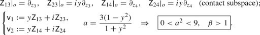
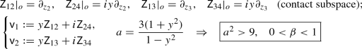
(N.6-2 tubular cases) In \({{\mathbb {R}}}^3\), consider the affine surface \(u = y\exp (x) + \exp (\alpha x)\), for \(\alpha \in {{\mathbb {R}}}\backslash \{ -1,0,1,2 \}\). Proceeding similarly as in Example 4.4 yields the complex ILC structure
Then \(({\tilde{z}}_1,{\tilde{z}}_2,{\tilde{w}}) = (\exp (\frac{z_1}{2}),z_2\exp (\frac{z_1}{2}),cw)\), where \(c = 2^{\frac{1}{\alpha -1}}\), transforms the above system to
From [9, Table 1], this is equivalent (for \(\alpha \ne 0,1\)) to an N.6-2 model with \(\mu = \alpha \) and \(\kappa = \alpha -2\). The parameters \((\mu ,\kappa )\) are related to Cartan basis parameters (a, b) by [9, Table 12]:
Hence, \(\mu = \alpha \) and \(\kappa = \alpha -2\) forces for \(\alpha \in {{\mathbb {R}}}\backslash \{ -1,0,1,2 \}\) the relation displayed in Table 7:
For \(u = xy + \exp (x)\), we get ILC structure \(w_{11} = \frac{1}{2} e^{w_2}, \, w_{12} = \frac{1}{2}, \, w_{22} = 0\). Then \(({\tilde{z}}_1,{\tilde{z}}_2,{\tilde{w}}) = (\frac{z_1}{2},\frac{z_2}{2},\frac{w}{2}- \frac{z_1z_2}{4})\) transforms it to the N.6-2 model in [9, Table 1] with \(\mu = \kappa = \infty \), which is the same as \(b^2 = a^2 = -4\) [9, Table 12]. Similarly, \(u = y\exp (x) - \frac{x^2}{2}\) yields the system \(w_{11} = \frac{1}{2} (w_1 + \ln (w_2) - 1), \, w_{12} = \frac{1}{2} w_2,\, w_{22} = 0\). Then \(({\tilde{z}}_1,{\tilde{z}}_2,{\tilde{w}}) = (e^{\frac{z_1}{2}}, \frac{z_2}{2}\exp (\frac{z_1}{2}), \frac{w}{2}+\frac{(z_1)^2}{8})\) transforms this to the N.6-2 model with \(\mu =0, \kappa = -2\), i.e. \(b^2 = a^2 = \frac{1}{2}\).
It remains to describe the tubular cases corresponding to \(b^2 = a^2 \in (-4,0]\). For \(\beta \in {{\mathbb {R}}}\), consider \(u\cos (x) + y\sin (x) = \exp (\beta x)\). Replacing (x, y, u) by \((\frac{ix}{2},i(y+u),-y+u)\) maps this to \(u e^{-x/2} - y e^{x/2} = e^{\beta i x/2}\), or \(u = y e^x + e^{\alpha x}\) with \(\alpha = \frac{\beta i + 1}{2}\). We get to (4.16) as above, which yields \(b^2 = a^2 = -\frac{4\beta ^2}{\beta ^2+9}\). This yields the classification on the third line from the end of Table 7.
Example 4.10
In the D.6-2 case, consider the affine surface \(u = y^2 + \epsilon x^\alpha \) for \(x > 0\) and \(\alpha \in {{\mathbb {R}}}\backslash \{ 0, 1, 2 \}\). Following the procedure above, we get \(\mu = \frac{\alpha -2}{\alpha -1}\), where \(\mu \) is the parameter appearing in [9, Table 1, D.6-2]. Since \(\mu = \frac{6(a-1)}{3a-4}\) from [9, Table 12], we get \(a = \frac{2}{3}(\frac{\alpha +1}{\alpha }) \in {{\mathbb {R}}}\backslash \{ \frac{2}{3}, \frac{4}{3}, 1 \}\). From Table 6, we have \(\tau = -\frac{(3a-2)(a-1)}{9} = \frac{2(\alpha -2)}{27\alpha ^2}\), and for \(\rho = \pm 1\) the anti-involution \(\varphi ^{(\rho )}\) for D.6-2 in Table 6 yields a definite structure if and only if \(\rho \tau > 0\), i.e. \(\rho (\alpha -2) > 0\). On the other hand, we find that the 2nd fundamental form of \(u = y^2 + \epsilon x^\alpha \) is definite if and only if \(\epsilon \alpha (\alpha -1) > 0\). This forces \(\rho = \epsilon \) for \(\alpha \in (0,1) \cup (2,\infty )\) and \(\rho = -\epsilon \) for \(\alpha \in (-\infty ,0) \cup (1,2)\), i.e. \(\rho = \epsilon \,\mathrm {sgn}(\alpha (\alpha -1)(\alpha -2))\). In terms of a, this is the same (after simplification) as \( \rho = \epsilon \,\mathrm {sgn}( (3a-2)(3a-4)(a-1))\).
As in the above examples, we can consider other affine-homogeneous surfaces in \({{\mathbb {R}}}^3\) listed in [7]. According to [7], all of those with at least 3-dimensional affine symmetry algebra are given by cylinders with homogeneous base, quadrics, or the Cayley surface \(u=xy-\frac{x^3}{3}\). In almost all cases, these give surfaces with degenerate 2nd fundamental form or lead to flat CR structures. The only exceptions are the (pseudo-)spheres \(u^2 + \epsilon _1 x^2 + \epsilon _2 y^2 = 1\), where we can take \((\epsilon _1,\epsilon _2) \in \{ \pm (1,1),(1,-1) \}\). These lead to complex ILC structures of type D.6-3 (with \(a^2 = 9\) and symmetry algebra \(\mathfrak {so}(3,{{\mathbb {C}}}) \ltimes {{\mathbb {C}}}^3\)) and their corresponding CR real forms. In all other cases in [7], the affine symmetry dimension is precisely 2.
Remark 4.11
Note all surfaces in [7] give multiply-transitive tubular hypersurfaces, e.g.
-
\(u = x(\alpha \ln x + \ln y)\): type I when \(\alpha \ne -1,0,8\); type II when \(\alpha = 8\); type N when \(\alpha =0\); Levi-degenerate when \(\alpha =-1\).
-
\(xu =y^{2} \pm x^{\alpha }\): type I when \(\alpha \ne 0,1,2,4\); type D when \(\alpha =0,4\); Levi-degenerate when \(\alpha =1,2\).
Recall from Table 6 that all the CR structures in our classification are of type N or D.
We conclude this section by showing that the dimensions of the affine symmetry subalgebras, i.e. \(\mathrm{dim}(N({{\mathfrak {a}}})/{{\mathfrak {a}}})\), listed in Table 2 are maximal among all possible tubular realizations \(({{\mathfrak {a}}},\varphi )\). It remains to prove this for those cases in Table 2 with \(\mathrm{dim}(N({{\mathfrak {a}}})/{{\mathfrak {a}}}) \le 1\). See Tables 7 and 8 for models.
N.7-2. Here, \({{\mathfrak {s}}}= \mathfrak {sl}(2,{{\mathbb {C}}}) \ltimes (V_2 \oplus V_0)\), where \(V_k\) denotes the standard \((k+1)\)-dimensional irreducible \(\mathfrak {sl}(2,{{\mathbb {C}}})\)-module. (Here, \(V_2 \oplus V_0\) is an abelian ideal in the symmetry algebra.) Then \(\varphi ^{(+1)}\) and \(\varphi ^{(-1)}\) (see Table 6) lead to CR structures with \(\mathfrak {sl}(2,{{\mathbb {R}}}) \ltimes (V_2 \oplus V_0)\) and \(\mathfrak {su}(2) \ltimes (V_2 \oplus V_0)\) symmetry respectively.Footnote 4 It suffices to consider the latter case. We will show \(N({{\mathfrak {a}}})={{\mathfrak {a}}}\) always.
Since \({{\mathfrak {a}}}\subset {{\mathfrak {s}}}\) is self-centralizing, then \({{\mathfrak {a}}}\not \subset V_2\oplus V_0\) or else \({{\mathfrak {c}}}({{\mathfrak {a}}}) \supset V_2\oplus V_0\). The projection of \({{\mathfrak {a}}}\) on \(\mathfrak {su}(2)\) must be 1-dimensional. Consider \(x+v\in {{\mathfrak {a}}}\), where \(0 \ne x\in \mathfrak {su}(2)\) and \(v\in V_2\oplus V_0\). From the centralizer of \(x+v\), we get \({{\mathfrak {a}}}=\langle x+v,v_0,v_1\rangle \), where \(v_0\) spans \(V_0\) and \(0 \ne v_1\in V_2\) is in the kernel of x. Since \(x+v\) is semisimple and has 1-dimensional kernels on \(\mathfrak {su}(2)\) and \(V_2\), then \(\mathrm{dim}(N({{\mathfrak {a}}})) = 3\).
D.7. When \(a\ne \pm \frac{3}{4}\), the symmetry algebra is \({{\mathfrak {s}}}=\mathfrak {sl}(2,{{\mathbb {C}}})\times \mathfrak {sl}(2,{{\mathbb {C}}})\times {{\mathbb {C}}}\). All real forms of \({{\mathfrak {s}}}\) are determined by real forms of the semisimple part, namely \(\mathfrak {sl}(2,{{\mathbb {R}}})\times \mathfrak {sl}(2,{{\mathbb {R}}})\), \(\mathfrak {sl}(2,{{\mathbb {R}}})\times \mathfrak {su}(2)\), \(\mathfrak {su}(2)\times \mathfrak {su}(2)\), and \(\mathfrak {sl}(2,{{\mathbb {C}}})_{{\mathbb {R}}}\). Any 3-dimensional abelian subalgebra \({{\mathfrak {a}}}\subset {{\mathfrak {s}}}\) is generated by the center and one element \(T_j\) from each copy of \(\mathfrak {sl}(2,{{\mathbb {C}}})\), and \(N({{\mathfrak {a}}})\) is the intersection of the normalizers of \(T_j\). The element \(T_j\) has a 2-dimensional normalizer in the corresponding copy of \(\mathfrak {sl}(2,{{\mathbb {C}}})\) if it is nilpotent and 1-dimensional otherwise. Since \(\mathfrak {su}(2)\) consists of semisimple elements, we immediately see that \(\mathrm{dim}( N({{\mathfrak {a}}})) \le 5\) for the \(\mathfrak {sl}(2,{{\mathbb {R}}})\times \mathfrak {sl}(2,{{\mathbb {R}}})\) and \(\mathfrak {sl}(2,{{\mathbb {C}}})_{{\mathbb {R}}}\) cases, \(\mathrm{dim}( N({{\mathfrak {a}}})) \le 4\) for the \(\mathfrak {sl}(2,{{\mathbb {R}}})\times \mathfrak {su}(2)\) case, and finally \(\mathrm{dim}( N({{\mathfrak {a}}}))=3\) for the \(\mathfrak {su}(2)\times \mathfrak {su}(2)\) case.
When \(a=\pm \frac{3}{4}\), \({{\mathfrak {s}}}= \mathfrak {sl}(2,{{\mathbb {C}}}) \times {{\mathfrak {r}}}\), where \({{\mathfrak {r}}}\) has relations \([S,X]=X,\,\, [S,Y]=-Y,\,\, [X,Y]=Z\). Since \({{\mathfrak {c}}}({{\mathfrak {a}}})={{\mathfrak {a}}}\), and \({{\mathfrak {r}}}\) contains no 3-dimensional abelian subalgebra, then \({{\mathfrak {a}}}\) must be spanned by the central element Z, a non-central element \(R \in {{\mathfrak {r}}}\), and some \(T \in \mathfrak {sl}(2,{{\mathbb {C}}})\). The normalizer in \({{\mathfrak {r}}}\) of R is at most 3-dimensional in \({{\mathfrak {r}}}\), and the normalizer in \(\mathfrak {sl}(2,{{\mathbb {C}}})\) of T has dimension 2 if T is nilpotent and 1 if T is semisimple. Hence, if the real form of \({{\mathfrak {s}}}\) contains \(\mathfrak {so}(3)\) (namely, for \(\varphi ^{\epsilon _1,1}\)), then \(\mathrm{dim}(N({{\mathfrak {a}}})) \le 4\).
N.6-2. Tubular CR structures arise when \(b^2 = a^2 \in {{\mathbb {R}}}\). Using the parameter redundancy (see Sect. 3), we can always assume that \(b = a\). In the generic case, \(b^2 = a^2 \in {{\mathbb {R}}}\backslash \{ -4, \frac{1}{2} \}\), consider the basis of \({{\mathfrak {s}}}\) from [9, Table 12]. This satisfies \(\kappa = \mu -2\) and the commutator relations in [9, Table 9]:
with \({{\mathfrak {n}}}= \langle N_1,N_2,N_3,N_4\rangle \) an abelian ideal. From (4.15), we have \(\mu = \frac{1}{2} + \frac{3a}{2\sqrt{a^2+4}} \in {{\mathbb {C}}}\setminus \{0,1 \}\), and according to [9, Table 13] models parametrised by \(\mu \) and \(1-\mu \) are equivalent.
To show \(\mathrm{dim}(N({{\mathfrak {a}}})) \le 4\) for any affine realization \({{\mathfrak {a}}}\subset {{\mathfrak {s}}}\), it suffices to show \(\mathrm{dim}(N({{\mathfrak {a}}}) \cap {{\mathfrak {n}}}) \le 2\). First note that \({{\mathfrak {a}}}\not \subset {{\mathfrak {n}}}\), since otherwise its centralizer would contain \({{\mathfrak {n}}}\) (4-dimensional). Therefore \({{\mathfrak {a}}}\) must contain an element \(T = \alpha S_1 + \beta S_2 + v\), where \(v \in {{\mathfrak {n}}}\) and \((\alpha ,\beta ) \ne (0,0)\). Since \({{\mathfrak {a}}}\) is abelian, then \((\mathrm{Ad}_T|_{N({{\mathfrak {a}}})})^2 = 0\). Since \(\mathrm{Ad}_T|_{{\mathfrak {n}}}\) is diagonalizable, then \(\ker (\mathrm{Ad}_T|_{{\mathfrak {n}}})^2 = \ker (\mathrm{Ad}_T|_{{\mathfrak {n}}})\). Hence, \(N({{\mathfrak {a}}}) \cap {{\mathfrak {n}}}\subset \ker (\mathrm{Ad}_T|_{{\mathfrak {n}}})\). We want \(\mathrm{dim}(\ker (\mathrm{Ad}_T|_{{\mathfrak {n}}})) \le 2\). The eigenvalues of \(\mathrm{Ad}_T|_{{\mathfrak {n}}}\) are
and \(\mathrm{dim}(\ker (\mathrm{Ad}_T|_{{\mathfrak {n}}})) \ge 3\) would contradict \((\alpha ,\beta ) \ne (0,0)\). Thus, \(\mathrm{dim}(N({{\mathfrak {a}}}) \cap {{\mathfrak {n}}}) \le 2\) follows.
The two remaining cases are \(a^2=b^2=-4\) and \(a^2=b^2=\frac{1}{2}\). The former admits an affinely homogeneous tubular representation, while the latter has structure constants (see [9, Table 12]):
(Again, \({{\mathfrak {n}}}= \langle N_1,N_2,N_3,N_4\rangle \) is an abelian ideal.) The condition \(\mathrm{dim}(\ker (\mathrm{Ad}_T|_{{\mathfrak {n}}})) \le 2\) easily follows.
N.6-1 \((a^2=2)\). From [9, Table 9], we have abelian \({{\mathfrak {n}}}= \langle N_2,N_3,N_4,N_5\rangle \) and commutators
As above, \({{\mathfrak {a}}}\not \subset {{\mathfrak {n}}}\), and \({{\mathfrak {a}}}\) contains \(T=\alpha S+\beta N_1 + v\), where \(v\in {{\mathfrak {n}}}\) and \((\alpha ,\beta ) \ne (0,0)\). Since \(\mathrm{dim}({{\mathfrak {a}}}) = 3\), then \(\mathrm{dim}({{\mathfrak {a}}}\cap {{\mathfrak {n}}}) \ge 1\), and \(\mathrm{Ad}_T|_{{{\mathfrak {a}}}\cap {{\mathfrak {n}}}} = 0\). This forces \(\alpha =0\). Hence, \({{\mathfrak {a}}}\) must be spanned by \(N_1 + t_2 N_2 + t_3 N_3, N_4,N_5\). Note \(N_3 \in N({{\mathfrak {a}}})\), so \(\mathrm{dim}(N({{\mathfrak {a}}})) \ge 4\). But \(\mathrm{dim}(N({{\mathfrak {a}}})) \le 4\), since
indicates that \(\gamma S + \delta N_2 \in N({{\mathfrak {a}}})\) only when \(\gamma = \delta = 0\).
5 Real forms of ILC D.6-3 models
5.1 Real form symmetry algebras
The ILC D.6-3 models [9, Table 7] admit a single essential parameter \(a^2 \in {{\mathbb {C}}}\backslash \{ 0 \}\). In the Cartan basis, the D.6-3 structure equations are:
When \(a^2=9\) (labelled D.6-3\(_\infty \) in [9]), the symmetry algebra is \({{\mathfrak {s}}}\cong \mathfrak {so}(3,{{\mathbb {C}}}) \ltimes {{\mathbb {C}}}^3\), the model admits a tubular representation, and all CR real forms are given in Table 8. (The 2nd fundamental form for \(u^2 + \epsilon _1 x^2 + \epsilon _2 y^2 = 1\) has definite signature if and only if \(\epsilon _1 \epsilon _2 > 0\), so \((\epsilon _1,\epsilon _2) = (1,-1)\) corresponds to \(\varphi _1\) since this yields an indefinite structure (Table 6). The \(\varphi _2^{(\pm 1)}\) cases are then identified from (5.1) and the semisimple part of the symmetry algebra.)
All models with \(a^2 \in {{\mathbb {C}}}\backslash \{ 0, 9 \}\) are non-tubular with symmetry algebra \({{\mathfrak {s}}}\cong \mathfrak {sl}(2,{{\mathbb {C}}}) \times \mathfrak {sl}(2,{{\mathbb {C}}}) \cong \mathfrak {so}(4,{{\mathbb {C}}})\). Recall that the real forms of \(\mathfrak {so}(4,{{\mathbb {C}}})\) and their Killing form signatures are
Using our list of the D.6-3 admissible anti-involutions \(\varphi \) (Table 6), we obtain a basis of the real form \({{\mathfrak {s}}}^\varphi \) of \(\mathfrak {so}(4,{{\mathbb {C}}})\), and classify \({{\mathfrak {s}}}^\varphi \) from the signature of its Killing form (Table 3). Note that these CR structures only arise when \(a^2 \in {{\mathbb {R}}}\backslash \{ 0, 9 \}\) (Theorem 4.8).
5.2 Cartan hypersurfaces
Let \((\cdot ,\cdot )\) denote a non-degenerate symmetric bilinear form on \({{\mathbb {C}}}^4\). The Lie group \(\text {O}(4,{{\mathbb {C}}})\) preserves \({{\mathcal {Q}}}= \{ [z] : (z,z) = 0 \} \subset {{\mathbb {C}}}{{\mathbb {P}}}^3\) and acts transitively on \({{\mathbb {C}}}{{\mathbb {P}}}^3 \backslash {{\mathcal {Q}}}\). Define \(A = \begin{pmatrix} (z,z) &{} (z,\bar{z}) \\ (z,\bar{z}) &{} (\bar{z},\bar{z}) \end{pmatrix}\). The (complex) scaling \(z \mapsto \lambda z\) induces \(A \mapsto LA\bar{L}\), where \(L = {\text {diag}}(\lambda ,{\bar{\lambda }})\). On \({{\mathbb {C}}}{{\mathbb {P}}}^3 \backslash {{\mathcal {Q}}}\), this scaling action has invariant \(\alpha := \frac{(z,\bar{z})^2}{(z,z)(\bar{z},\bar{z})}\). We will fix \((\cdot ,\cdot )\) that is non-degenerate and \({{\mathbb {R}}}\)-valued on \({{\mathbb {R}}}^4 \subset {{\mathbb {C}}}^4\), so that \((\bar{z},\bar{z}) = \overline{(z,z)}\). In this case, \(\beta := \frac{(z,\bar{z})}{|(z,z)|} \in {{\mathbb {R}}}\) is invariant under complex scalings, and \(\alpha = \beta ^2\). We refer to the real hypersurfaces of \({{\mathbb {C}}}{{\mathbb {P}}}^3 \backslash {{\mathcal {Q}}}\) uniformly described by
as Cartan hypersurfaces. A precise list of inequivalent such structures is given in Table 4. Restricting \(z = (z_1,\ldots ,z_4)^\top \) in (5.2) to the standard affine coordinate chart \(z_1 = 1\) on \({{\mathbb {C}}}{{\mathbb {P}}}^3\) recovers Loboda’s models [11, Eqs. (2.8) and (2.9)], [13, eqns (6)&(7)], which are generalizations of models found by Cartan [3, Eq. (10)]. In this subsection, we match these models with their corresponding ILC structures and identify the associated anti-involutions.
Given \(z = (z_1,\ldots ,z_4)^\top \), consider \((z,z) = \epsilon _1 (z_1)^2 + \cdots + \epsilon _4 (z_4)^2\), where \(\epsilon _j = \pm 1\). Then \(\mathfrak {so}(4,{{\mathbb {C}}})\) can be identified with the \({{\mathbb {C}}}\)-span of \({\mathsf {Z}}_{jk} = \epsilon _j z_j \partial _{z_k} - \epsilon _k z_k \partial _{z_j}\), where \(1 \le j < k \le 4\). Their \({{\mathbb {R}}}\)-span is identified with the real form of \(\mathfrak {so}(4,{{\mathbb {C}}})\) that preserves the restriction of \((\cdot ,\cdot )\) to \({{\mathbb {R}}}^4 \subset {{\mathbb {C}}}^4\). Let us classify real 5-dimensional orbits of each of \(\text {O}(4),\text {O}(3,1),\text {O}(2,2)\) on \({{\mathbb {C}}}{{\mathbb {P}}}^3 \backslash {{\mathcal {Q}}}\). (Here, we take \(\text {O}(3,1)\) corresponding to \(\epsilon _1 = \epsilon _2 = \epsilon _3 = +1\) and \(\epsilon _4 = -1\), etc.) Given [z] in such an orbit, \(v = \mathfrak {Re}(z)\) and \(w = \mathfrak {Im}(z)\) span a real 2-plane \(\Pi \) in \({{\mathbb {R}}}^4\) (otherwise the orbit is only 3-dimensional). Since \((c_1 + c_2 i)(v + w i) = c_1 v - c_2 w + (c_2 v + c_1 w)i\), then the new real and imaginary parts satisfy
This quadratic in \(c_1,c_2\) has discriminant \(((v,v) - (w,w))^2 + 4(v,w)^2 \ge 0\). Thus, using complex multiplication, we may assume that \((v,w) = 0\). Hence, \(0 \ne (z,z) = (v+wi,v+wi) = (v,v) - (w,w)\) so that only real (\(c_2 = 0\)) or purely imaginary (\(c_1 = 0\)) rescalings preserve this orthogonality.
Suppose that \((\cdot ,\cdot )|_\Pi \) is non-degenerate. Applying each real orthogonal group and the residual rescalings to the orthogonal pair \(\{ v,w \}\), we obtain the following normal forms for \([z] \in {{\mathbb {C}}}{{\mathbb {P}}}^3 \backslash {{\mathcal {Q}}}\):
-
(1)
\(\Pi \) positive-definite: \(z = (1,iy,0,0)\), where \(0< y < 1\). Then \(\beta = \frac{1+y^2}{1-y^2} > 1\).
-
(2)
\(\Pi \) indefinite: assuming signature \((+++\,-)\) or \((++-\,-)\), we have
-
\(z = (1,0,0,iy)\), where \(0< y < 1\) \(\quad \Rightarrow \quad \beta = \frac{1-y^2}{1+y^2}\) satisfies \(0< \beta < 1\);
-
\(z = (iy,0,0,1)\), where \(0< y < 1\) \(\quad \Rightarrow \quad \beta = -\frac{1-y^2}{1+y^2}\) satisfies \(-1< \beta < 0\).
-
The negative-definite case can be made positive-definite by absorbing a sign in (5.2) into \(\beta \).
For a given orbit M with basepoint a normal form \(o = [z]\) above, the standard complex structure J on \({{\mathbb {C}}}{{\mathbb {P}}}^3\) induces \(H = TM \cap J(TM)\) and a CR structure. For each such M, we determine a Cartan basis \(e_1,\ldots , e_6\) of \(\mathfrak {so}(4,{{\mathbb {C}}})\), i.e. so that the ILC D.6-3 structure equations are satisfied. (Each basis element will be a \({{\mathbb {C}}}\)-linear combination of \({\mathsf {Z}}_{ij}\).) We begin by choosing a generator \(e_6\) for the (complex) isotropy \({{\mathfrak {k}}}\subset \mathfrak {so}(4,{{\mathbb {C}}})\) so that \(\mathrm{ad}(e_6)\) has eigenvalues \((+1,-1,-1,+1)\) on \(({{\mathfrak {e}}}+{{\mathfrak {v}}})/{{\mathfrak {k}}}\) (which corresponds to H). We then choose a basis \(e_1,\ldots ,e_4\) adapted to the \(\pm i\)-eigenspaces for J, then rescale the basis so that \([e_1,e_2] = -[e_3,e_4] \in {{\mathfrak {k}}}\), and finally choose \(e_5\) to satisfy the remaining structure equations. We summarize the results below. In each case, with respect to the basis \(e_1,\ldots ,e_4 \,\mathrm{mod}\ {{\mathfrak {k}}}\), we have \(J = {\text {diag}}\left( \begin{pmatrix} 0 &{} -y\\ \frac{1}{y} &{} 0 \end{pmatrix}, \begin{pmatrix} 0 &{} -y\\ \frac{1}{y} &{} 0 \end{pmatrix}\right) \). We also define \({\mathsf {v}}_1,{\mathsf {v}}_2\) so that
-
(1)
\(\Pi \) positive-definite for \(\text {O}(4),\text {O}(3,1),\text {O}(2,2)\): \(o = [(1,iy,0,0)^\top ]\), \(0< y < 1\). Isotropy: \({\mathsf {Z}}_{34}\).
-
\(\text {O}(4)\)-case: \(\rho = \sqrt{\frac{3}{4(1+y^2)}}\), \({\left\{ \begin{array}{ll} e_1 = \rho (\overline{{\mathsf {v}}_1} - i \overline{{\mathsf {v}}_2}), \, e_2 = \rho (\overline{{\mathsf {v}}_1} + i \overline{{\mathsf {v}}_2}), \\ e_3 = \rho ({\mathsf {v}}_1 + i {\mathsf {v}}_2),\, e_4 = \rho ({\mathsf {v}}_1 - i {\mathsf {v}}_2), \\ e_5 = \frac{3iy}{1+y^2} {\mathsf {Z}}_{12},\, e_6 = i{\mathsf {Z}}_{34} \end{array}\right. }\)
-
\(\text {O}(3,1)\)-case: \(\rho = \sqrt{\frac{3}{4(1+y^2)}}\), \({\left\{ \begin{array}{ll} e_1 = \rho (\overline{{\mathsf {v}}_1} -\overline{{\mathsf {v}}_2}), \, e_2 = \rho (\overline{{\mathsf {v}}_1} + \overline{{\mathsf {v}}_2}), \\ e_3 = \rho ({\mathsf {v}}_1 + {\mathsf {v}}_2),\, e_4 = \rho ({\mathsf {v}}_1 - {\mathsf {v}}_2), \\ e_5 = \frac{3iy}{1+y^2} {\mathsf {Z}}_{12},\, e_6 = {\mathsf {Z}}_{34} \end{array}\right. }\)
-
\(\text {O}(2,2)\)-case: \(\rho = \sqrt{\frac{-3}{4(1+y^2)}}\), \({\left\{ \begin{array}{ll} e_1 = \rho (\overline{{\mathsf {v}}_1} + i\overline{{\mathsf {v}}_2}), \, e_2 = \rho (\overline{{\mathsf {v}}_1} - i\overline{{\mathsf {v}}_2}), \\ e_3 = \rho ({\mathsf {v}}_1 - i {\mathsf {v}}_2),\, e_4 = \rho ({\mathsf {v}}_1 + i {\mathsf {v}}_2), \\ e_5 = \frac{3iy}{1+y^2} {\mathsf {Z}}_{12},\, e_6 = i{\mathsf {Z}}_{34} \end{array}\right. }\)
-
-
(2)
\(\Pi \) indefinite for \(\text {O}(3,1),\text {O}(2,2)\): \(o = [(1,0,0,iy)^\top ]\), \(0< y < 1\). Isotropy: \({\mathsf {Z}}_{23}\).
-
\(\text {O}(3,1)\)-case: \(\rho = i\sqrt{\frac{3}{4(1-y^2)}}\), \({\left\{ \begin{array}{ll} e_1 = \rho (\overline{{\mathsf {v}}_1} - i \overline{{\mathsf {v}}_2}),\, e_2 = \rho (\overline{{\mathsf {v}}_1} + i \overline{{\mathsf {v}}_2}),\\ e_3 = \rho ({\mathsf {v}}_1 + i {\mathsf {v}}_2),\, e_4 = \rho ({\mathsf {v}}_1 - i {\mathsf {v}}_2),\\ e_5 = \frac{3iy}{1-y^2} {\mathsf {Z}}_{14},\, e_6 = i {\mathsf {Z}}_{23} \end{array}\right. }\)
Anti-involution: \(\varphi _2^{(-1)}\), since \(\mathfrak {so}(3,1) = \mathrm {span}_{{\mathbb {R}}}\{ i(e_1 + e_3), e_1 - e_3, i(e_2 + e_4), e_2 - e_4, i e_5, ie_6 \}\).
-
\(\text {O}(2,2)\)-case: \(\rho = \sqrt{\frac{3}{4(y^2-1)}}\), \({\left\{ \begin{array}{ll} e_1 = \rho (\overline{{\mathsf {v}}_1} - \overline{{\mathsf {v}}_2}),\, e_2 = \rho (\overline{{\mathsf {v}}_1} + \overline{{\mathsf {v}}_2}),\\ e_3 = \rho ({\mathsf {v}}_1 + {\mathsf {v}}_2),\, e_4 = \rho ({\mathsf {v}}_1 - {\mathsf {v}}_2),\\ e_5 = \frac{3iy}{1-y^2} {\mathsf {Z}}_{14},\, e_6 = {\mathsf {Z}}_{23} \end{array}\right. }\)
-
-
(3)
\(\Pi \) indefinite for \(\text {O}(3,1)\): \(o = [(iy,0,0,1)^\top ]\), \(0< y < 1\). Isotropy: \({\mathsf {Z}}_{23}\).

-
\(\text {O}(3,1)\)-case: \(\rho = \sqrt{\frac{3}{4(1-y^2)}}\), \({\left\{ \begin{array}{ll} e_1 = \rho (\overline{{\mathsf {v}}_1} - i \overline{{\mathsf {v}}_2}),\, e_2 = \rho (\overline{{\mathsf {v}}_1} + i \overline{{\mathsf {v}}_2}),\\ e_3 = \rho ({\mathsf {v}}_1 + i {\mathsf {v}}_2),\, e_4 = \rho ({\mathsf {v}}_1 - i {\mathsf {v}}_2),\\ e_5 = \frac{3iy}{1-y^2} {\mathsf {Z}}_{14},\, e_6 = i{\mathsf {Z}}_{23} \end{array}\right. }\)
Anti-involution: \(\varphi _2^{(+1)}\), since \(\mathfrak {so}(3,1) = \mathrm {span}_{{\mathbb {R}}}\{ e_1 + e_3, i(e_1 - e_3), e_2 + e_4, i(e_2 - e_4), i e_5, ie_6 \}\). By flipping the signature, we can write this as an \(\text {O}(1,3)\) case with \(0< \beta < 1\).
-
\(\text {O}(2,2)\)-case: Flipping the signature reduces this to the earlier \(\text {O}(2,2)\) case.
-


A posteriori, we have  , so all of Table 3 is covered except for the models arising from \(\varphi _3\). The complete list of inequivalent Cartan hypersurfaces (5.2) is given in Table 4. This classification is consistent with that of Loboda [11, Eqs. (2.8) and (2.9)], [13, Eqs. (6) and (7)].
5.3 Quaternionic models
It remains to describe the CR structures associated with the anti-involution \(\varphi _3\), which are all indefinite type and admit \(\mathfrak {so}^*(4)\) symmetry. To our knowledge, these models are new. While \(\mathfrak {so}^*(4)\) is customarily defined via a skew-Hermitian form \(\eta \) on \({{\mathbb {H}}}^2\), where \({{\mathbb {H}}}\) is the quaternions, we will instead focus on the special isomorphism \(\mathfrak {so}^*(4) \cong \mathfrak {sl}(2,{{\mathbb {R}}}) \times \mathfrak {su}(2)\). In doing so, we will work with a particularly simple representation of this Lie algebra and the choice of \(\eta \) will arise naturally from this. In contrast, if we were to fix a choice of \(\eta \) first, the resulting realization of \(\mathfrak {so}^*(4)\) could be quite complicated.
Recall that \({{\mathbb {H}}}\) is the associative \({{\mathbb {R}}}\)-algebra with \({{\mathbb {R}}}\)-basis \(1,\mathbf{i},\mathbf{j},\mathbf{k}\), standard relations \(\mathbf{i}\mathbf{j}= \mathbf{k},\, \mathbf{i}^2 = \mathbf{j}^2 = \mathbf{k}^2 = -1\), conjugation satisfying \(\overline{q_1 q_2} = \overline{q_2} \,\overline{q_1}\), and norm \(|q|^2 = q{\overline{q}} = {\overline{q}} q\). Let \(\text {SU}(2)\) denote the unit quaternions, which act on \({{\mathbb {H}}}\) on the left. Let \({\widehat{\mathrm {SL}}}(2,{{\mathbb {R}}})\) denote \(2\times 2\) real matrices with determinant \(\pm 1\), which act on \({{\mathbb {R}}}^2\). The group \(S = {{\widehat{\mathrm {SL}}}}(2,{{\mathbb {R}}}) \times \text {SU}(2)\) acts on the external tensor product \({{\mathbb {R}}}^2 \otimes _{{\mathbb {R}}}{{\mathbb {H}}}\), and we identify this naturally with \({{\mathbb {H}}}^2\). This identification is S-equivariant if for \(q = \begin{pmatrix} q_1\\ q_2 \end{pmatrix} \in {{\mathbb {H}}}^2\), we declare that \(A \in {\widehat{\mathrm {SL}}}(2,{{\mathbb {R}}})\) and \(q_0 \in \text {SU}(2)\) each act by multiplication on the left, with the latter identified with \({\text {diag}}(q_0,q_0)\). (These actions commute.) While \({{\mathbb {H}}}^2\) is naturally a right \({{\mathbb {H}}}\)-vector space, it will be more important for us to consider it as a \({{\mathbb {C}}}\)-vector space by restricting this right action to \({{\mathbb {C}}}:= \{ 1s + \mathbf{i}t : s,t \in {{\mathbb {R}}}\} \subset {{\mathbb {H}}}\). (This in particular distinguishes the imaginary unit \(\mathbf{i}\).) We will be interested in the 5-dimensional S-orbits in \({{\mathbb {C}}}{{\mathbb {P}}}^3 \cong {{\mathbb {P}}}_{{\mathbb {C}}}({{\mathbb {H}}}^2)\).
There exists an S-invariant skew-Hermitian form on \({{\mathbb {H}}}^2\) (unique up to a real scaling) given by \(\eta (q,w) = \overline{q_1} w_2 - \overline{q_2} w_1\), and this is valued in \(\mathfrak {Im}({{\mathbb {H}}})\). Let \(\eta (q,q) = \mathbf{i}b + \mathbf{j}\mu \), for \(b \in {{\mathbb {R}}}\) and \(\mu \in {{\mathbb {C}}}\). Given \(\lambda \in {{\mathbb {C}}}\), \(\eta (q\lambda ,q\lambda ) = {\bar{\lambda }}\eta (q,q)\lambda \), hence \((b,\mu ) \mapsto (b|\lambda |^2, \mu \lambda ^2)\). Writing \(q = \begin{pmatrix} z_1 + \mathbf{j}z_2\\ z_3 + \mathbf{j}z_4 \end{pmatrix}\) for \(z_j \in {{\mathbb {C}}}\),
Note that \({{\mathcal {Q}}}^\#= \{ [q] : \mathfrak {Re}(\mathbf{i}\eta (q,q)) = 0 \}\) is the flat (indefinite) CR structure \(\mathfrak {Im}(\overline{z_1} z_3 + \overline{z_2} z_4) = 0\), so we exclude \(b=0\). We will also exclude the \(\mu = 0\) case (see below), since this yields only 4-dimensional S-orbits. When \(b\mu \ne 0\), we have the complex scaling invariant \(\gamma = \frac{b}{|\mu \mathbf{k}|} \in {{\mathbb {R}}}\backslash \{ 0 \}\). Since \(b = -\mathfrak {Re}(\mathbf{i}\eta (q,q))\) and \(\mu = -\mathbf{j}\eta (q,q) - b\mathbf{k}\), the S-orbits in \({{\mathbb {C}}}{{\mathbb {P}}}^3 \backslash {{\mathcal {Q}}}^\#\) satisfy
Equivalently, \(\mathfrak {Im}(\overline{z_1} z_3 + \overline{z_2} z_4) = \gamma |\mathbf{i}\mathfrak {Re}(z_1 \overline{z_3} + z_2 \overline{z_4}) - (z_1 z_4 - z_2 z_3) \mathbf{k}|\), which further simplifies to
Let us find representatives for the S-orbits on \({{\mathbb {C}}}{{\mathbb {P}}}^3 \backslash {{\mathcal {Q}}}^\#\). Given \(0 \ne q \in {{\mathbb {H}}}^2\), we may swap \(q_1\) and \(q_2\) if necessary to assume \(q_1 \ne 0\), and then use \(\text {SU}(2)\) and a real rescaling to assume \(q_1 = 1\). Using \(\begin{pmatrix} 1 &{} 0\\ -\mathfrak {Re}(q_2) &{} 1\end{pmatrix} \in \mathrm {SL}(2,{{\mathbb {R}}})\), we may assume \(\mathfrak {Re}(q_2) = 0\). Using \(e^{\mathbf{i}\phi } \in \text {SU}(2)\) and the right \({{\mathbb {C}}}\)-action by \(e^{-\mathbf{i}\phi }\), we can replace \(q_2 \mapsto e^{\mathbf{i}\phi } q_2 e^{-\mathbf{i}\phi }\), so choose \(\phi \) to normalize \(q_2 = \mathbf{i}s + \mathbf{j}t\), where \(s,t \in {{\mathbb {R}}}\) with \(t \le 0\). Finally, use \({\text {diag}}(\lambda , \frac{1}{\lambda }) \in \mathrm {SL}(2,{{\mathbb {R}}})\) and right multiplication by \(\frac{1}{\lambda }\) to normalize \(q_2\) to be of unit length. Thus, we have \(q_2 = \mathbf{i}e^{\mathbf{k}\theta }\), for some fixed \(0 \le \theta < \pi \). For \(q = \begin{pmatrix} 1\\ \mathbf{i}e^{\mathbf{k}\theta } \end{pmatrix}\), we have \(\eta (q,q) = 2\mathbf{i}e^{\mathbf{k}\theta }\). When \(\theta = \frac{\pi }{2}\) or 0, we have \(b=0\) or \(\mu = 0\), so we exclude these. The (S-equivariant) conjugation arising from the identification \({{\mathbb {H}}}^2 = {{\mathbb {C}}}^4\), i.e. \(\widetilde{u+\mathbf{j}v} = \bar{u} + \mathbf{j}\bar{v}\) (where \(u,v \in {{\mathbb {C}}}^2\)), maps \(\begin{pmatrix} 1\\ \mathbf{i}e^{\mathbf{k}\theta } \end{pmatrix} \mapsto \begin{pmatrix} 1\\ \mathbf{i}e^{\mathbf{k}(\pi -\theta )} \end{pmatrix}\). Thus, we can restrict to \(\gamma = \cot (\theta ) > 0\), or equivalently require \(\theta \in (0,\frac{\pi }{2})\). Hence, we can restrict to \(0< \theta < \frac{\pi }{2}\), which is in 1-1 correspondence with \(\gamma = \cot \theta \in {{\mathbb {R}}}^+\).
The elements \(\mathbf{i},\mathbf{j},\mathbf{k}\) span \(\mathfrak {su}(2)\), and let \({\mathsf {H}}= \begin{pmatrix} 1 &{}0\\ 0 &{} -1\end{pmatrix},{\mathsf {X}}=\begin{pmatrix} 0 &{}1\\ 0 &{} 0\end{pmatrix},{\mathsf {Y}}=\begin{pmatrix} 0 &{}0\\ 1 &{} 0\end{pmatrix}\) span \(\mathfrak {sl}(2,{{\mathbb {R}}})\). Consider the S-orbit M through \([q] \in {{\mathbb {C}}}{{\mathbb {P}}}^3 \backslash {{\mathcal {Q}}}^\#\), where \(q = \begin{pmatrix} 1\\ \mathbf{i}e^{\mathbf{k}\theta } \end{pmatrix}\) for \(0< \theta < \frac{\pi }{2}\). Then [q] has 1-dimensional isotropy \({{\mathfrak {k}}}\) spanned by \({\mathsf {T}}= -\mathbf{i}e^{\mathbf{k}\theta } + {\mathsf {X}}- {\mathsf {Y}}\). (Note \({{\mathfrak {k}}}= \mathrm {span}_{{\mathbb {R}}}\{ \mathbf{i}, {\mathsf {X}}- {\mathsf {Y}}\}\) when \(\theta = 0\).) The complex structure J on \({{\mathbb {C}}}{{\mathbb {P}}}^3\) is induced from right multiplication by \(\mathbf{i}\) on \({{\mathbb {H}}}^2\). Defining
the elements \({\mathsf {w}}_1 \cdot q,\ldots ,{\mathsf {w}}_4 \cdot q\, \,\mathrm{mod}\ [q]\) span the contact subspace \(H_{[q]} \subset T_{[q]} M\). In this basis, \(J = {\text {diag}}(\begin{pmatrix} 0 &{} -1\\ 1 &{} 0\end{pmatrix}, \begin{pmatrix} 0 &{} -1\\ 1 &{} 0\end{pmatrix})\). In \(\mathrm {span}_{{\mathbb {C}}}\{ {\mathsf {w}}_1,\ldots , {\mathsf {w}}_4, {\mathsf {T}}\}\), define
Here we have distinguished the scalar i from the Lie algebra element \(\mathbf{i}\). The \(-i\)-eigenspace \({{\mathfrak {v}}}/ {{\mathfrak {k}}}\) for J is spanned by \(\{ {\mathsf {v}}_1, {\mathsf {v}}_2 \} \,\mathrm{mod}\ {\mathsf {T}}\), while the \(+i\)-eigenspace \({{\mathfrak {e}}}/ {{\mathfrak {k}}}\) is spanned by \(\{ \overline{{\mathsf {v}}_1},\overline{{\mathsf {v}}_2}\} \,\mathrm{mod}\ {\mathsf {T}}\). (We caution that this conjugation fixes each of \({\mathsf {w}}_1,\ldots ,{\mathsf {w}}_4,{\mathsf {T}}\) and conjugates the scalars. It is distinct from the conjugation on \({{\mathbb {H}}}\), and that associated with \({{\mathbb {H}}}^2 = {{\mathbb {C}}}^4\).) The ILC D.6-3 structure equations are satisfied if we take
In particular,  classifies the corresponding ILC D.6-3 structure.
6 Hypersurfaces of Winkelmann type
Generalizing (1.1), we say that a real hypersurface in \({{\mathbb {C}}}^3\) is of Winkelmann type if in some holomorphic coordinate system \((z_1,z_2,w)\), it is given by
where F is an arbitrary real-valued analytic function. These all admit the symmetries
They span an abelian Lie algebra that induces a (holomorphic) foliation of \({{\mathbb {C}}}^3\) by 2-dimensional holomorphic hypersurfaces \(z_1={\text {const}}\) outside of the singular set \(z_1=0\).
Complexifying (6.1), we get the following complex hypersurfaces in \({{\mathbb {C}}}^3\times {\bar{{{\mathbb {C}}}}}^3\):
Regarding \(w = w(z_1,z_2)\), we obtain \(w_1 := \frac{\partial w}{\partial z_1} = a_2 + 2iF_{z_1}(z_1,a_1)\) and \(w_2 := \frac{\partial w}{\partial z_2} = -a_1\). Differentiate with respect to \(z_1\) and \(z_2\) once more and eliminate the parameters \((a_1,a_2,b)\). Making the variable change \(z_2 \mapsto -z_2\), we arrive at the PDE system
The harmonic curvature [9, (3.3)] is of type N if \(F_{z_1 z_1 w_2 w_2}\ne 0\). Let us consider the specific Winkelmann type hypersurfaces given in Table 5.
Writing out (6.3) for \(F(z_1,\bar{z}_1) = (z_1)^\alpha (\bar{z}_1)^{{\bar{\alpha }}}\), we obtain
Using a constant rescaling of \(z_2\), and relabelling, we can bring (6.4) into the same form as that listed in [9, Table 1] for the N.6-2 models with \(\mu = {\bar{\alpha }}\) and \(\kappa = \alpha - 2\). The \(F(z_1,\bar{z}_1) = \exp (z_1)\exp (\bar{z}_1)\) and \(F(z_1,\bar{z}_1) = \ln (z_1) \ln (\bar{z}_1)\) cases are handled similarly. The corresponding ILC N.6-2 models have \(\mu = \kappa = \infty \) for the former and \((\mu ,\kappa ) = (0,-2)\) for the latter, c.f. [9, Table 1].
As discussed in Sect. 3, the N.6-2 models are described using \((a,b) \in {{\mathbb {C}}}^2\), with \((a^2,b^2)\) being essential parameters. Using (4.15) with \(\mu = {\bar{\alpha }}\) and \(\kappa = \alpha - 2\), we find that for \(\alpha \in {{\mathbb {C}}}\setminus \{ -1, 0, 1, 2 \}\):
(The \(\alpha = -1\) and \(\alpha = 2\) cases lead to the ILC N.8 model.) The \(b^2 = a^2 \in \{ -4, \frac{1}{2} \}\) cases were described in Example 4.9. From Sect. 4, the \(b^2 = a^2 \in {{\mathbb {R}}}\) cases are tubular (see Table 7 for models).
Proposition 6.1
The hypersurfaces of Winkelmann type given in Table 5 are models for all real forms of the complex ILC N.6-2 structures. Their (6-dimensional) CR symmetry algebras are never transitive outside of these hypersurfaces.
Proof
From Table 6, \(b^2 = \bar{a}^2 \in {{\mathbb {C}}}\) are the parameter values that yield underlying CR structures, and in each case there is a unique structure. Thus, Table 5 gives a complete classification as claimed.
For the second claim, let us fix a basepoint \(o \in {{\mathbb {C}}}^3\) and suppose that \(z_1|_o = c+di\), where \(c,d \in {{\mathbb {R}}}\). Then \(N_1 - c N_2 - dN_3 + (c^2+d^2) N_4\) vanishes at o. Thus, these symmetry algebras have at most 5-dimensional orbits at all points in \({{\mathbb {C}}}^3\). \(\square \)
7 Transitivity of the symmetry algebra
In this section, we prove Theorem 1.3. According to [14, Cor.6.36], \(\mathrm {Sym}(M)\) is transitive on an open subset of \({{\mathbb {C}}}^3\) if and only if \(\mathrm {Sym}(M^c)\) is transitive on an open subset of \({{\mathbb {C}}}^3\times {\bar{{{\mathbb {C}}}}}^3\).
Proposition 7.1
Suppose \(M\subset {{\mathbb {C}}}^3\) is locally transitive, and let \(({{\mathfrak {s}}},{{\mathfrak {k}}};{{\mathfrak {e}}},{{\mathfrak {v}}})\) be an algebraic model of the ILC structure (E, V) on \(M^c\). Then \(\mathrm {Sym}(M^c)\) is transitive on a non-empty open subset of \({{\mathbb {C}}}^3\times {\bar{{{\mathbb {C}}}}}^3\) if and only if for some \(T\in {\text {Int}}({{\mathfrak {s}}})\), we have:
Proof
Assume that \({{\mathfrak {s}}}=\mathrm {Sym}(M^c)\) is transitive on a non-empty open subset of \({{\mathbb {C}}}^3\times {\bar{{{\mathbb {C}}}}}^3\) and fix a point (z, a) in this subset. Then the projection of \({{\mathfrak {s}}}\) on \({{\mathbb {C}}}^3\) is transitive on an open subset of \({{\mathbb {C}}}^3\) containing \(z\in {{\mathbb {C}}}^3\). The isotropy subalgebra of this action at z is conjugate to \({{\mathfrak {v}}}\) by means of some inner automorphism \(T_1 \in {\text {Int}}({{\mathfrak {s}}})\). Similarly, the projection of \({{\mathfrak {s}}}\) to \({\bar{{{\mathbb {C}}}}}^3\) is transitive at \(a\in {\bar{{{\mathbb {C}}}}}^3\) with the isotropy subalgebra equal to \(T_2({{\mathfrak {e}}})\) for some \(T_2\in {\text {Int}}({{\mathfrak {s}}})\).
Note that \({{\mathfrak {s}}}\) is transitive at (z, a) if and only if the projection of \(T_1({{\mathfrak {v}}})\) to \({\bar{{{\mathbb {C}}}}}^3\) is transitive at \(a\in {{\mathbb {C}}}^3\), or, similarly, if the projection of \(T_2({{\mathfrak {e}}})\) to \({{\mathbb {C}}}^3\) is transitive at \(z\in {{\mathbb {C}}}^3\). Both these conditions are equivalent to the equality \(T_1({{\mathfrak {v}}})+T_2({{\mathfrak {e}}})={{\mathfrak {s}}}\). Applying \(T_2^{-1}\) to both sides of this equality we get \({{\mathfrak {e}}}+T({{\mathfrak {v}}})={{\mathfrak {s}}}\), where \(T=T_2^{-1}T_1\). \(\square \)
Corollary 7.2
The symmetry algebra \({{\mathfrak {s}}}= \mathrm {Sym}(M^c)\) is transitive on a non-empty open subset of \({{\mathbb {C}}}^3\times {\bar{{{\mathbb {C}}}}}^3\) if and only if the set of \(\epsilon \in {{\mathbb {C}}}\) satisfying:
is non-empty for any \(X\in {{\mathfrak {s}}}\) not contained in \({{\mathfrak {e}}}+{{\mathfrak {v}}}\).
Proof
Fix \(X \in {{\mathfrak {s}}}\backslash ({{\mathfrak {e}}}+ {{\mathfrak {v}}})\), and decompose \({{\mathfrak {s}}}\) into a direct sum of linear subspaces \(V_1\oplus {{\mathbb {C}}}X \oplus V_2\), where \(V_1\subset {{\mathfrak {e}}}\) and \(V_2\subset {{\mathfrak {v}}}\). It is well-known that the exponential map:
is locally biholomorphic in a neighborhood of 0. Taking \(T= \exp (X_1)\exp (\epsilon X)\exp (X_2)\) in (7.1) and multiplying both sides by \(\exp (-X_1)\) we get:
But by construction \(\exp (-X_1)({{\mathfrak {e}}})={{\mathfrak {e}}}\) and \(\exp (X_2)({{\mathfrak {v}}})={{\mathfrak {v}}}\). \(\square \)
Corollary 7.3
If \({{\mathfrak {s}}}\) has a non-trivial center, then \({{\mathfrak {s}}}\) is not transitive at any point of \({{\mathbb {C}}}^3\times {\bar{{{\mathbb {C}}}}}^3\).
Proof
Let Z be any central element in \({{\mathfrak {s}}}\). Since the subalgebra \({{\mathfrak {k}}}\) is effective, then \(Z\notin {{\mathfrak {k}}}\). Recall that Levi non-degeneracy of \(M\subset {{\mathbb {C}}}^3\) implies that the bilinear form:
is non-degenerate. Hence, it follows that Z does not lie in \({{\mathfrak {e}}}+{{\mathfrak {v}}}\). But it is obvious that \(\exp (\epsilon Z)({{\mathfrak {v}}})={{\mathfrak {v}}}\) for any \(\epsilon \in {{\mathbb {C}}}\), and \({{\mathfrak {s}}}\) is not transitive according to Corollary 7.2. \(\square \)
This proposition implies that the local transitivity of \(\mathrm {Sym}(M^c)\) on \({{\mathbb {C}}}^3 \times {\bar{{{\mathbb {C}}}}}^3\), and hence the local transitivity of \(\mathrm {Sym}(M)\) on \({{\mathbb {C}}}^3\), is a property of the algebraic model \(({{\mathfrak {s}}},{{\mathfrak {k}}};{{\mathfrak {e}}},{{\mathfrak {v}}})\) itself and does not depend on the particular realization of this model in local coordinates.
Transitivity off the hypersurface is well-known in the maximally symmetric and Winkelmann hypersurface cases [23]. Consider all remaining cases. For N.7-2, D.6-1, and D.7, \({{\mathfrak {s}}}\) has non-trivial center, so these are ruled out by Corollary 7.3. (See also Example 4.4 where it is computed explicitly as a Lie algebra of vector fields on \({{\mathbb {C}}}^3 \times {\bar{{{\mathbb {C}}}}}^3\).)
The remaining cases have 6-dimensional symmetry, so it suffices to exhibit a relation amongst the symmetry vector fields. For N.6-1, tubular realizations are given in Table 7 and share the symmetries \(N_1=i\partial _{z_2}\), \(N_2=i\partial _w\), \(N_3=\partial _{z_2}+z_1\partial _w\), and \(N_4=iz_1\partial _{z_2}+i\frac{z_1^2}{2}\partial _w\). Letting \(z_1=a+bi\), we have \(aN_1+\frac{a^2+b^2}{2}N_2-bN_3-N_4=0\). The N.6-2 cases were similarly ruled out in Proposition 6.1. The D.6-2 realizations (see Table 8) share the symmetries \(N_1=i\partial _{z_2}\), \(N_2=i\partial _w\), \(N_3=\partial _{z_2}+2z_2\partial _w\), and \(N_4=iz_2\partial _{z_2}+iz_2^2\partial _w\). Letting \(z_2=c+di\), we have \(cN_1+(c^2+d^2)N_2-dN_3-N_4=0\). For D.6-3 (\(a^2 = 9\)), the symmetries of the tubular models in Table 8 have an obvious dependency. Finally, for D.6-3 (\(a^2 \ne 9\)), see § 5 where the orbits of \(\mathrm {Sym}(M)\) are described explicitly.
Notes
Private communication with Robert Bryant.
Flatness refers to being locally equivalent under point transformations to the trivial PDE system \(u_{jk} = 0\).
The map \((e_1,\ldots ,e_6) \mapsto (\epsilon _1 e_1, \epsilon _2 e_2, \epsilon _1 e_3, \epsilon _2 e_4, e_5, \epsilon _1 \epsilon _2 e_6)\), where \(\epsilon _1 = \pm 1\) and \(\epsilon _2 = \pm 1\), induces the parameter change \((a,b) \mapsto (\epsilon _1 a, \epsilon _2 b)\) and \(\epsilon \mapsto \epsilon _1 \epsilon _2 \epsilon \). This is an automorphism only when \(a=b=0\).
We have abused notation here: \(V_2\) refers to the adjoint representation of \(\mathfrak {sl}(2,{{\mathbb {R}}})\) or \(\mathfrak {su}(2)\) respectively, and \(V_0\) is the trivial 1-dimensional representation.
As noted in the Introduction, a D.6-1 real form is missing from Loboda’s list.
The ODE \(u'' = \frac{3(u')^2}{2u} + cu^3\) as listed in [15, Table 7] is flat when \(c=0\) (so 8 symmetries) and all \(c \ne 0\) are equivalent via scalings, so we normalized \(c=1\). Similar normalizations were done in the other cases.
References
Baouendi, M.S., Ebenfelt, P., Rothschild, L.P.: Real Submanifolds in Complex Space and Their Mappings, Princeton Math. Ser., vol. 47. Princeton University Press, Princeton (1999)
Čap, A.: On left invariant CR structures on \(\text{ SU }(2)\). Arch. Math. 42(Supplement), 185–195 (2006)
Cartan, É.: Sur la géométrie pseudo-conforme des hypersurfaces de l’espace de deux variables complexes II. Ann. Scuola Norm. Sup. Pisa Cl. Sci. (2) 1(4), 333–354 (1932)
Cartan, É.: Sur la géométrie pseudo-conforme des hypersurfaces de l’espace de deux variables complexes. Ann. Mat. Pura Appl. 11(1), 17–90 (1933)
Cartan, É.: Sur les domaines bornés homogenes de l’espace de \(n\) variables complexes. Abh. Math. Sem. Hamb. Univ. 11, 116–162 (1935)
Chern, S.S., Moser, J.K.: Real hypersurfaces in complex manifolds. Acta Math. 133, 219–271 (1974)
Doubrov, B., Komrakov, B., Rabinovich, M.: Homogeneous surfaces in the three-dimensional affine geometry. In: Geometry and Topology of Submanifolds, VIII. Proceedings of the international meeting on geometry of submanifolds, Brussels, Belgium, July 13–14, 1995 and Nordfjordeid, Norway, July 18–August 7, 1995, pp. 168–178. World Scientific, Singapore (1996)
Doubrov, B.M., Komrakov, B.P.: Classification of homogeneous submanifolds in homogeneous spaces. Lobachevskii J. Math. 3, 19–38 (1999)
Doubrov, B., Medvedev, A., Th, D.: Homogeneous integrable Legendrian contact structures in dimension five. J. Geom. Anal. (2019). https://doi.org/10.1007/s12220-019-00219-x
Ezhov V.V., Loboda, A.V., Schmalz, G.: Canonical form of a fourth-degree polynomial in a normal equation of a real hypersurface in \({\mathbb{C}}^3\), Mat. Zametki 66(4), 624–626 (1999). Translation in Math. Notes 66(3–4), 513–515 (2000)
Loboda, A.V.: Homogeneous real hypersurfaces in \({\mathbb{C}}^3\) with two-dimensional isotropy groups. Tr. Mat. Inst. Steklova 235 (2001). Anal. i Geom. Vopr. Kompleks. Analiza, pp. 114–142. (Russian) translation in Proc. Steklov Inst. Math. 235(4 ), 107–135 (2001)
Loboda, A.V.: Homogeneous strictly pseudoconvex hypersurfaces in \({\mathbb{C}}^3\) with two-dimensional isotropy groups. Mat. Sb. 192(12), 3–24 (2001); (Russian) translation in Sb. Math. 192(11–12), 1741–1761 (2001)
Loboda, A.V.: Determination of a homogeneous strictly pseudoconvex surface from the coefficients of its normal equation. Math. Notes 73(3), 419–423 (2003)
Merker, Joël: Lie symmetries and CR geometry. J. Math. Sci. 154(6), 817–922 (2008)
Olver, P.J.: Symmetry, Invariants, and Equivalence. Springer, New York (1995)
Piatetski-Shapiro, I.I.: On a problem proposed by É. Cartan. Dokl. Akad. Nauk SSSR 124, 272–273 (1959)
Segre, B.: Questioni geometriche legate colla teoria delle funzioni di due variabili complesse. Rendic. del Seminario Mat. della R. Università di Roma, n. 24, p. 51 (1931)
Segre, B.: Intorno al problem di Poincaré della rappresentazione pseudo-conforme. Rend. Acc. Lincei 13, 676–683 (1931)
Sukhov, A.: Segre varieties and Lie symmetries. Math. Z. 238(3), 483–492 (2001)
Sukhov, A.: On transformations of analytic CR-structures. Izv. Math. 67(2), 303–332 (2003)
Tanaka, N.: On the pseudo-conformal geometry of hypersurfaces of the space of \(n\) complex variables. J. Math. Soc. Japan 14, 397–429 (1962)
Webster, S.M.: On the mapping problem for algebraic real hypersurfaces. Invent. Math. 43(1), 53–68 (1977)
Winkelmann, J.: The Classification of Three-dimensional Homogeneous Complex Manifolds. Lecture Notes in Mathematics, vol. 1602. Springer, Berlin (1995)
Acknowledgements
Open Access funding provided by UiT The Arctic University of Norway. The authors gratefully acknowledge the use of the DifferentialGeometry package in Maple. This project was supported by the Austrian Science Fund (FWF project M1884-N35 for D.T.), as well as the Tromsø Research Foundation.
Author information
Authors and Affiliations
Corresponding author
Additional information
Publisher's Note
Springer Nature remains neutral with regard to jurisdictional claims in published maps and institutional affiliations.
Appendices
Appendix A: Representative admissible anti-involutions
In Table 6, we classify all representative admissible anti-involutions (see Sect. 3) for all non-flat 5-dimensional multiply-transitive complex ILC structures. Each anti-involution is expressed in the same basis used in [9, Tables 6–8].

Appendix B: Tubular hypersurfaces
In Tables 7 and 8, we give the complete (local) classification of (non-flat) homogeneous tubular hypersurfaces in \({{\mathbb {C}}}^3\) with non-degenerate Levi form, organized according to Petrov type. The third column classification is given in terms of our ILC classification and the anti-involutions presented in Table 6. (No anti-involution is specified if there is a unique one.) We let \(\epsilon = \pm 1\) here, and write \(x = \mathfrak {Re}(z_1), y = \mathfrak {Re}(z_2)\), and \(u = \mathfrak {Re}(w)\). CR parameter redundancies are indicated, e.g. \(\alpha \sim -\alpha \).
By Theorem 4.8, the structures excluded from this list are D.6-3 \((a^2 \in {{\mathbb {R}}}\backslash \{ 0, 9 \})\) and N.6-2 (\(b^2 = {\overline{a}}^2 \in {{\mathbb {C}}}\backslash {{\mathbb {R}}}\)). These are discussed in Sects. 5 and 6 respectively.
Remark B.1
For \(u = y\exp (x) + \exp (\alpha x)\) in the N.6-2 case, \(\alpha =0,1\) lead to the flat model, while \(\alpha =-1,2\) give alternative descriptions of the N.8 model.
Remark B.2
In the first three D.7 cases, \(\alpha = -1\) yields the flat model. This is also true in the D.6-2 case when \(\alpha = 0,1,2\).
Appendix C: Loboda’s models
In Table 9, we give a dictionary between Loboda’s classifications and our results. The first two series of examples describe all non-degenerate hypersurfaces with 7-dimensional symmetry algebra and indefinite [11] or definite [12] Levi form. The last seven rows correspond to hypersurfaces with 6-dimensional symmetry algebra and positive-definite Levi form found in [13].Footnote 5 All equations here use the notation \(z_j=x_j+i y_j\) and \(w=u+iv\).
Loboda’s models are not in the tubular form (4.2), but we find the corresponding complex ILC structures as in Sect. 2.1 (by replacing barred variables with parameters), see for instance Example 2.2. We then proceed similarly as in the examples in Sect. 4 to identify these models in our classification.
Appendix D: Homogeneous 3-dimensional CR structures
It is well-known that all Levi non-degenerate real hypersurfaces in \({{\mathbb {C}}}^2\) admit at most an 8-dimensional symmetry algebra. Moreover, the submaximal symmetry dimension is 3 and É. Cartan gave a complete local classification of all such (homogeneous) models [4, bottom of p.70]. Here we outline how this classification can be alternatively derived from the well-known classification of (complex) 2nd order ODE that are homogeneous (in fact, simply-transitive, so the isotropy subalgebra is everywhere trivial) under point symmetries [15, Table 7].Footnote 6 The list is:
-
(A): \(u'' = \frac{3(u')^2}{2u} + u^3\)
-
(B): \(u'' = 6 uu' - 4 u^3+c (u'-u^2)^{3/2}\), where \(c \in {{\mathbb {C}}}\backslash \{ 0 \}; \,\,\, c \sim -c\)
-
(C): \(u'' = (u')^\gamma \), where \(\gamma \in {{\mathbb {C}}}\backslash \{ 0,1,2,3 \}; \quad \gamma \sim 3-\gamma \)
-
(D): \(u'' = e^{-u'}\)
All parameters that yield equivalent models are indicated, e.g. \(\gamma \sim 3-\gamma \). Set \(p=u'\) below.
Label | Point symmetries | Lie algebra structure |
|---|---|---|
(A) | \(\begin{array}{l} e_1 = \partial _x, \quad e_2 = x \partial _x - u \partial _u - 2p\partial _p,\\ e_3 = x^2 \partial _x - 2xu\partial _u - (4xp+2u)\partial _p \end{array}\) | \(\begin{array}{l} [e_1,e_2] = e_1\\ {} [e_1,e_3] = 2e_2\\ {} [e_2,e_3] = e_3 \end{array}\) |
(B) | \(\begin{array}{l} e_1 = \partial _x, \quad e_2 = x \partial _x - u \partial _u - 2p\partial _p,\\ e_3 = x^2 \partial _x - (2xu+1)\partial _u - (4xp+2u)\partial _p + \frac{c}{2} e_2 - e_1 \end{array}\) | \(\begin{array}{l} [e_1,e_2] = e_1\\ {} [e_1,e_3] = \frac{c}{2} e_1 + 2e_2\\ {} [e_2,e_3] = 2e_1 - \frac{c}{2} e_2 + e_3 \end{array} \) |
(C) | \(\begin{array}{l} e_1 = (\gamma -1) x \partial _x + (\gamma -2) u \partial _u - p\partial _p\\ e_2 = \partial _x, \,\,\, e_3 = \partial _u, \\ \end{array}\) | \(\begin{array}{l} [e_1,e_2] = -(\gamma -1)e_2\\ {} [e_1,e_3] = -(\gamma -2) e_3\\ {} [e_2,e_3] = 0 \end{array}\) |
(D) | \(\begin{array}{l} e_1 = \partial _x, \,\,\, e_2 = \partial _u,\\ e_3 = x\partial _x + (x+u)\partial _u + \partial _p \end{array}\) | \(\begin{array}{l} [e_1,e_2] = 0\\ {} [e_1,e_3] = e_1+e_2\\ {} [e_2,e_3] = e_2 \end{array}\) |
For each model, pick a general point o, identify the (1-dimensional) subalgebras \({{\mathfrak {e}}}\) and \({{\mathfrak {v}}}\) of the point symmetry algebra \({{\mathfrak {s}}}\) corresponding to the line fields \(E = \mathrm {span}\{ \partial _x + p\partial _u + f\partial _p\}\) and \(V = \mathrm {span}\{ \partial _p \}\) at o, and then classify all anti-involutions of \({{\mathfrak {s}}}\) that swap \({{\mathfrak {e}}}\) and \({{\mathfrak {v}}}\). (This is tedious, but straightforward.) All representative such admissible anti-involutions are given in Table 10.
It is easy to recognize tubular CR structures from Table 10. These arise from (C) and (D), since each admits a unique abelian subalgebra \({{\mathfrak {a}}}\) (namely, \(\mathrm {span}\{ e_2, e_3 \}\) and \(\mathrm {span}\{ e_1, e_2 \}\) respectively) that is complementary to both \({{\mathfrak {e}}}\) and \({{\mathfrak {v}}}\), and satisfies the properties given in Sect. 4. (None exists for (B) since \({{\mathfrak {s}}}\cong \mathfrak {sl}(2,{{\mathbb {C}}})\).) The listed anti-involutions preserve \({{\mathfrak {a}}}\) in these cases, and since \(\mathrm{dim}( N({{\mathfrak {a}}}) / {{\mathfrak {a}}}) = 1\), the base curve for the tubular CR hypersurface model is affine homogeneous. The classification (up to affine equivalence) of locally homogeneous curves in the affine plane consists of lines, quadrics, and the curves given below. (See Example 1 in [8], particularly p.32 there.)
Real affine curve \(F(x,u) = 0\) | Classification | CR syms of \(F(\mathfrak {Re}(z),\mathfrak {Re}(w)) = 0\) beyond \(i\partial _{z}, i\partial _{w}\) |
|---|---|---|
\(\begin{array}{l} u = x^a\\ (a \in {{\mathbb {R}}}\backslash \{ 0,\frac{1}{2},1,2 \}; \,\, a \sim \frac{1}{a}) \end{array}\) | \(\text{(C) }, \, \gamma = \frac{a-2}{a-1},\,\, \varphi _1\) | \(z\partial _z + a w\partial _w\) |
\(u = \ln (x)\) | \(\text{ flat } \text{ model }\) | \(\text{8 } \text{ CR } \text{ symmetries }\) |
\(u = x\ln (x)\) | \(\text{(D) }\) | \(z\partial _z + (z+w)\partial _w \) |
\(\begin{array}{c} x^2 + u^2 = \exp (b \arg (x+iu)) \\ (b \in {{\mathbb {R}}}; \,\,\, b \sim -b) \end{array}\) | \(\text{(C) },\, \gamma = \frac{3}{2} \pm \frac{b}{4} i,\,\, \varphi _2\) | \((b z - 2w)\partial _z + (b w + 2 z) \partial _w\) |
Upon complexification (Sect. 2), \(u = \ln (x)\) leads to \(u_{xx} = -(u_x)^2\), which is equivalent to \({\tilde{u}}_{xx} = 0\) via \(({\tilde{x}},{\tilde{u}}) = (x,e^u)\), and hence this leads to the flat CR structure with 8 CR symmetries. On the other hand, \(u = x^a\) and \(u = x\ln (x)\) lead to the CR models underlying (C) (with \(\gamma = \frac{a-2}{a-1} \in {{\mathbb {R}}}\backslash \{ 0,1,2,3\}\) and anti-involution \(\varphi _1\)) and (D). This is not so straightforward for \(x^2 + u^2 = \exp (b\arg (x+iu))\), so we instead work abstractly and align the Lie algebra data. Letting
we have
On the other hand, the anti-involution \(\varphi _2\) from case (C) has real fixed point set spanned by
Since we must have \(\gamma = \frac{3}{2} + ti\), then
To align the structures, take \(t = -\frac{b}{4}\). Clearly \((x,u) \mapsto (x,-u)\) induces the parameter redundancy \(b \mapsto -b\), so \(\gamma = \frac{3}{2} \pm \frac{b}{4} i\). Hence, all CR structures underlying (C) and (D) have been accounted for.
All ODE models for (B) admit \({{\mathfrak {s}}}= \mathfrak {sl}(2,{{\mathbb {C}}}) \cong \mathfrak {so}(3,{{\mathbb {C}}})\) symmetry. We show that all underlying CR structures are exhausted by the Cartan hypersurfaces \((z,\bar{z}) = \beta |(z,z)|\) as in (5.2). Since the classified anti-automorphisms for (B) are very complicated, we proceed in a different manner. Note that \({{\mathfrak {s}}}\) has two real forms: \(\mathfrak {sl}(2,{{\mathbb {R}}}) \cong \mathfrak {so}(2,1)\) and \(\mathfrak {su}(2) \cong \mathfrak {so}(3)\). For each, a left-invariant CR structure is uniquely determined by a two-dimensional subspace C with \([C,C] \not \subset C\), and a complex structure \(J:C\rightarrow C\). The subspace C is uniquely determined by its Killing perp \(C^{\perp }\). In \(\mathfrak {su}(2)\), \([C,C] \not \subset C\) always. In \(\mathfrak {sl}(2,{{\mathbb {R}}})\), \([C,C]\subset C\) if and only if \(C^{\perp }\) is spanned by a nilpotent element, and C is conjugate to the subalgebra of upper-triangular matrices in \(\mathfrak {sl}(2,{{\mathbb {R}}})\). (Exclude this last case.)
Identifying J with a \(2\times 2\) real matrix satisfying \(J^2 = -1\), we have \(J^2 - {\text {tr}}(J) J + \det (J) =0\). If \({\text {tr}}(J) \ne 0\), then J is a real scalar matrix, which cannot satisfy \(J^2 = -1\). Thus, \({\text {tr}}(J) = 0\) and \(\det (J) = 1\). Hence, \(J = \left( {\begin{matrix} a &{} b \\ c &{} -a \end{matrix}}\right) \) with \(a^2+bc=-1\), i.e. \(c = -\frac{a^2+1}{b}\).
Let us classify all \(J:C \rightarrow C\) up to automorphisms stabilizing C. For example, in \(\mathfrak {sl}(2,{{\mathbb {R}}})\) consider the case of \(C^\perp \) spanned by \(h = \left( {\begin{matrix} 1 &{} 0 \\ 0 &{} -1 \end{matrix}}\right) \). Then C has basis \(e_1 = \left( {\begin{matrix} 0 &{} 1 \\ -1 &{} 0 \end{matrix}}\right) \), \(e_2 = \left( {\begin{matrix} 0 &{} 1 \\ 1 &{} 0 \end{matrix}}\right) \), and \(\mathrm{Ad}_{\exp (th)}\) is represented in this basis by \(T= \left( {\begin{matrix}\cosh (2t) &{} \sinh (2t) \\ \sinh (2t) &{} \cosh (2t) \end{matrix}}\right) \). With J as above, we find that \(TJT^{-1}\) is anti-diagonal iff \(\tanh (4t) = \frac{2a}{b-c} = \frac{2ab}{a^2+b^2+1}\). This is valued in \((-1,1)\), so such t exists. Thus, J can always be brought to the form \(\left( {\begin{matrix}0 &{} -\alpha \\ 1/\alpha &{} 0 \end{matrix}}\right) \). Note that C is also stable under \(\mathrm{Ad}\left( {\begin{matrix} 0 &{} 1 \\ 1 &{} 0 \end{matrix}}\right) \). It induces the transformation \(e_1\mapsto -e_1\), \(e_2\mapsto e_2\) and thus the parameter equivalence \(\alpha \sim -\alpha \). Performing similar computations for other subspaces C, we get the following list of all algebraic models for case (B).
Real form of \(\mathfrak {sl}(2,{{\mathbb {C}}})\) | Basis of \(C^\perp \) | Basis of the contact plane C | Complex structure | Parameter equivalence |
|---|---|---|---|---|
\(\mathfrak {su}(2)\) | \(\begin{pmatrix} i &{} 0 \\ 0 &{} -i \end{pmatrix}\) | \(e_1 = \begin{pmatrix} 0 &{} 1 \\ -1 &{} 0 \end{pmatrix}, \,\, e_2 = \begin{pmatrix} 0 &{} i \\ i &{} 0 \end{pmatrix}\) | \(\begin{pmatrix} 0 &{} -\alpha \\ 1/\alpha &{} 0 \end{pmatrix}\) | \(\alpha \sim -\alpha , 1/\alpha \) |
\(\mathfrak {sl}(2,{{\mathbb {R}}})\) | \(\begin{pmatrix} 0 &{} 1 \\ -1 &{} 0 \end{pmatrix}\) | \(e_1 = \begin{pmatrix} 1 &{} 0 \\ 0 &{} -1 \end{pmatrix}, \,\, e_2 = \begin{pmatrix} 0 &{} 1 \\ 1 &{} 0 \end{pmatrix}\) | \(\begin{pmatrix} 0 &{} -\alpha \\ 1/\alpha &{} 0 \end{pmatrix}\) | \(\alpha \sim -\alpha , 1/\alpha \) |
\(\mathfrak {sl}(2,{{\mathbb {R}}})\) | \(\begin{pmatrix} 1 &{} 0 \\ 0 &{} -1 \end{pmatrix}\) | \(e_1 = \begin{pmatrix} 0 &{} 1 \\ -1 &{} 0 \end{pmatrix}, \,\, e_2 = \begin{pmatrix} 0 &{} 1 \\ 1 &{} 0 \end{pmatrix}\) | \(\begin{pmatrix} 0 &{} -\alpha \\ 1/\alpha &{} 0 \end{pmatrix}\) | \(\alpha \sim -\alpha \) |
The first of these cases is treated in detail in [2]. The two others are their non-compact analogues.
To construct the local models, we proceed as in Sect. 5.2 and just give a summary here. Given \(z = (z_1,z_2,z_3)^\top \), consider \((z,z) = \sum _{j=1}^3 \epsilon _j (z_j)^2\), where \(\epsilon _j = \pm 1\). Then \(\mathfrak {so}(3,{{\mathbb {C}}})\) is identified with the \({{\mathbb {C}}}\)-span of \({\mathsf {Z}}_{jk} = \epsilon _j z_j \partial _{z_k} - \epsilon _k z_k \partial _{z_j}\), where \(1 \le j < k \le 3\). Let \({{\mathcal {Q}}}= \{ [z] : (z,z) = 0 \}\). Given [z] in a real 3-dimensional orbit of \(\text {O}(3)\) or \(\text {O}(2,1)\) in \({{\mathbb {C}}}{{\mathbb {P}}}^2 \backslash {{\mathcal {Q}}}\), \(v = \mathfrak {Re}(z)\) and \(w = \mathfrak {Im}(z)\) span a real 2-plane \(\Pi \) in \({{\mathbb {R}}}^3\). Using complex multiplication, we can assume \((v,w) = 0\). Taking \((\cdot ,\cdot )|_\Pi \) non-degenerate, the following are normal forms for \([z] \in {{\mathbb {C}}}{{\mathbb {P}}}^2 \backslash {{\mathcal {Q}}}\) (which slightly differ from those given in Sect. 5.2):
-
(1)
\(\Pi \) is positive-definite and the signature of the scalar product (z, z) is \((+++)\) or \((++-)\): \(z = (1,iy,0)\), where \(0< y < 1\). Then \(\beta = \frac{1+y^2}{1-y^2} > 1\).
-
(2)
\(\Pi \) is indefinite: assuming signature \((++-)\), we have: \(z = (1,0,iy)\), where \(0 < y \ne 1\). Then \(\beta = \frac{1-y^2}{1+y^2}\) satisfies \(0< |\beta | < 1\).
Matching these orbits with the above algebraic models is straightforward. Fix the affine chart \((1,z_2,z_3)\) in \({{\mathbb {C}}}{{\mathbb {P}}}^2\). For case (1), the orbit of \(\text {O}(3)\) or \(\text {O}(2,1)\) has 3-dimensional real tangent space in \({{\mathbb {C}}}^2 \cong T_{[z]}{{\mathbb {C}}}{{\mathbb {P}}}^2\) given by \(\langle (1-y^2)\partial _{z_2}, \partial _{z_3}, iy \partial _{z_3}\rangle \). (The scaling \(z_1 \partial _{z_1} + z_2 \partial _{z_2} + z_3 \partial _{z_3}\) on \({{\mathbb {C}}}^3\) induces a trivial action on \({{\mathbb {C}}}{{\mathbb {P}}}^2\), so in the given chart, we can make the substitutions \(\partial _{z_1} = -z_2 \partial _{z_2} - z_3 \partial _{z_3}\) into \({\mathsf {Z}}_{jk}\).) Then \(C = \langle \partial _{z_3}, iy \partial _{z_3} \rangle \), and multiplication by i is represented by \(\left( {\begin{matrix} 0 &{} -y \\ 1/y &{} 0 \end{matrix}}\right) \) in this basis. The range \(0< y < 1\) matches with the first two cases in the table above (namely, set \(y=\alpha \)). Case (2) is handled similarly.
Rights and permissions
Open Access This article is licensed under a Creative Commons Attribution 4.0 International License, which permits use, sharing, adaptation, distribution and reproduction in any medium or format, as long as you give appropriate credit to the original author(s) and the source, provide a link to the Creative Commons licence, and indicate if changes were made. The images or other third party material in this article are included in the article’s Creative Commons licence, unless indicated otherwise in a credit line to the material. If material is not included in the article’s Creative Commons licence and your intended use is not permitted by statutory regulation or exceeds the permitted use, you will need to obtain permission directly from the copyright holder. To view a copy of this licence, visit http://creativecommons.org/licenses/by/4.0/.
About this article

Cite this article
Doubrov, B., Medvedev, A. & The, D. Homogeneous Levi non-degenerate hypersurfaces in \({{\mathbb {C}}}^3\). Math. Z. 297, 669–709 (2021). https://doi.org/10.1007/s00209-020-02528-2
Received:
Accepted:
Published:
Issue Date:
DOI: https://doi.org/10.1007/s00209-020-02528-2
Keywords
- Real hypersurfaces in complex manifolds
- Symmetry algebra
- Homogeneous
- Integrable Legendrian contact structures