Multifractal analysis of some multiple ergodic averages in linear Cookie-Cutter dynamical systems

Abstract

In this paper, we study the multiple ergodic averages of a locally constant real-valued function in linear Cookie-Cutter dynamical systems. The multifractal spectrum of these multiple ergodic averages is completely determined.

1 Introduction and statement of results

Let $T : X\rightarrow X$ be a continuous map on a compact metric space X. Let $f_{1},\ldots ,f_{\ell }$ $(\ell \ge 2)$ be $\ell$ bounded real-valued functions on X. The following multiple ergodic average

$$\begin{aligned} \frac{1}{n}\sum _{k=1}^nf_{1}(T^kx)f_2(T^{2k}x)\cdots f_{\ell }(T^{\ell k}x) \end{aligned}$$

is widely studied in ergodic theory by Furstenberg [9], Bourgain [2], Host and Kra [10], Bergelson, Host and Kra [1] and others. Fan, Liao and Ma [6] and Kifer [13] have independently studied such multiple ergodic averages from the point of view of multifractal analysis.

Later on, the multifractal analysis of multiple ergodic averages have attracted much attention. First works are done on symbolic spaces. Let $m\ge 2$ be an integer and $S=\{0,\ldots ,m-1\}$. Consider the symbolic space $\Sigma _m=S^{{\mathbb {N}}^*}$ endowed with the metric

$$\begin{aligned} d(x,y)=m^{-\min \{n,x_n\ne y_n\}}, \ \ \forall x, y\in \Sigma _m. \end{aligned}$$

The first object of study was the Hausdorff dimension of the following level sets ( [6])

$$\begin{aligned} E(\alpha )=\left\{ (x_k)_{k=1}^\infty \in \Sigma _2\ : \ \lim _{n\rightarrow \infty }\frac{1}{n}\sum _{k=1}^n x_kx_{2k}=\alpha \right\} ,\quad \alpha \in [0,1]. \end{aligned}$$

More generally we may consider the Hausdorff spectrum of the following level sets of multiple ergodic averages

$$\begin{aligned} E^\ell _\varphi (\alpha )=\left\{ (x_k)_{k=1}^\infty \in \Sigma _m\ : \ \lim _{n\rightarrow \infty }\frac{1}{n}\sum _{k=1}^n \varphi (x_k,x_{kq},\ldots , x_{kq^{\ell -1}})=\alpha \right\} ,\quad \alpha \in {\mathbb {R}}\end{aligned}$$

(1)

where $q\ge 2,\ell \ge 2$ are integers and $\varphi$ is a real-valued function defined on $\{0,\ldots ,m-1\}^\ell$. The level set $E(\alpha )$ then corresponds to the set $E^\ell _\varphi (\alpha )$ with special choice $q=2,\ell =2$ and $\varphi (x,y)=xy$. See the works of Kenyon, Peres and Solomyak [11, 12], Peres, Schmeling, Seuret and Solomyak [16] on some specific subsets of level sets $E(\alpha )$. See Peres and Solomyak [15] for the multifractal analysis of $E(\alpha )$. Fan, Schmeling and Wu [5, 8] have considered a class of functions $\varphi$ that are involved in (1). Fan, Schmeling and Wu [7] have also considered some similar averages called V-statistics.

All of the above mentioned results concentrated on the full shift dynamical system $(\Sigma _m, \sigma )$ where the Lyapunov exponent of the shift transformation is constant. Recently, Liao and Rams [14] performed the multifractal analysis of a class of special multiple ergodic averages for some systems with non-constant Lyapunov exponents. More precisely, they considered a piecewise linear map T on the unit interval with two branches. Let $I_0,I_1\subset [0,1]$ be two intervals with disjoint interiors. Suppose that for each $i\in \{0,1\}$, the restriction $T: I_i\rightarrow [0,1]$ is bijective and linear with slop $e^{\lambda _i}$, $\lambda _i >0$. Let $J_T$ be the repeller of T, i.e.

$$\begin{aligned}J_T:=\bigcap _{n=1}^\infty T^{-n}[0,1]. \end{aligned}$$

Then $(J_T,T)$ becomes a dynamical system. As in [5, 6, 15], Liao and Rams investigated the following sets

$$\begin{aligned} L(\alpha )=\left\{ x\in J_T : \ \lim _{n\rightarrow \infty }\frac{1}{n}\sum _{k=1}^n 1_{I_1}(T^kx)1_{I_1}(T^{2k}x)=\alpha \right\} \ \ (\alpha \in [0,1]). \end{aligned}$$

By adapting the method of [15], they obtained the Hausdorff spectrum of the above level sets $L(\alpha )$.

We point out that the methods used in [15] and [14] seem inconvenient to be generalized to other IFSs with many branches and more general potentials $\varphi$. Some more adaptive methods are needed to generalise Liao–Rams’ results. The aim of this paper is to use similar arguments as in [8] to extend Liao–Rams’ results to the situation that we describe below.

Let $I_0,\ldots ,I_{m-1}\subset [0,1]$ be m intervals with disjoint interiors. Let $T: \cup _{i=0}^{m-1}I_i\rightarrow [0,1]$ be such that the restriction $T_{|I_i}$ is bijective and linear with slope $e^{\lambda _i}$, $\lambda _i>0$ ($0\le i\le m-1$). Denote by $J_T$ the repeller of T.

Let $\ell \ge 2$ be an integer, and $\varphi$ be a function defined on $[0,1]^\ell$ taking real values. We assume that $\varphi$ is locally constant in the sense that $\varphi$ is constant on each hyper-rectangle $I_{i_1}\times I_{i_2}\times \cdots \times I_{i_\ell }$ $(0\le i_1,i_2,\ldots ,i_\ell \le m-1)$.

With an abuse of notation, we write

$$\begin{aligned} \varphi (a_1,a_2,\ldots ,a_\ell )=\varphi (i_i,i_2,\ldots ,i_\ell ) \end{aligned}$$

for all $(a_1,a_2,\ldots ,a_\ell )\in I_{i_1}\times I_{i_2}\times \cdots \times I_{i_\ell }$.

In this paper, we would like to study the following sets

$$\begin{aligned} L_\varphi (\alpha ):=\left\{ x\in J_T : \ \lim _{n\rightarrow \infty }\frac{1}{n}\sum \varphi (T^kx,T^{kq}x, \ldots , T^{kq^{\ell -1}}x)=\alpha \right\} ,\quad \alpha \in {\mathbb {R}}. \end{aligned}$$

Our aim is to determine the Hausdorff dimension of $L_\varphi (\alpha )$.

For simplicity of notation, we restrict ourselves to the case $\ell =2$ (the same arguments work for arbitrary $\ell \ge 2$ without any problem). For any $s,r\in {\mathbb {R}}$, consider the non-linear transfer operator ${\mathcal {N}}_{(s,r)}$ on ${\mathbb {R}}_+^m$ defined by

$$\begin{aligned} \left( {\mathcal {N}}_{(s,r)}{\underline{t}} \right) _i=\left( \sum _{j=0}^{m-1}e^{s\varphi (i,j)-r\lambda _j}t_j\right) ^{1/q},\ \ (i=0,\ldots ,m-1). \end{aligned}$$

(2)

for all ${\underline{t}} =(t_j)_{j=0}^{m-1}\in {\mathbb {R}}_+^m$. In [8], a family of similar operators ${\mathcal {N}}_{s}\ (s\in {\mathbb {R}})$ was defined.

Notice that the Lyapunov exponents $\lambda _j$’s are now introduced in the definition of ${\mathcal {N}}_{(s,r)}$. It will be shown in Proposition 1 (see Sect. 2) that the equation ${\mathcal {N}}_{(s,r)}{\underline{t}} ={\underline{t}}$ admits a unique strictly positive solution $(t_0(s,r),\ldots ,t_{m-1}(s,r))$. We then define the pressure function by

$$\begin{aligned} P(s,r)=(q-1)\log \sum _{j=0}^{m-1}t_j(s,r)e^{-r\lambda _j}. \end{aligned}$$

It will also be shown (Proposition 1) that P is real-analytic and convex, and even strictly convex if $\varphi$ is non-constant and the $\lambda _j$’s are not all the same.

Let A and B be the infimum and the supremum respectively of the set

$$\begin{aligned} \left\{ a\in {\mathbb {R}} :\ \exists (s,r)\in {\mathbb {R}}^2 \ \mathrm{such\ that } \ \frac{\partial P}{\partial s}(s,r)=a\right\} . \end{aligned}$$

(3)

Let $D_{\varphi }=\left\{ \alpha \in {\mathbb {R}}: L_{\varphi }(\alpha )\ne \emptyset \right\} .$ Our main result is as follows.

Theorem 1

Under the assumptions made above, we have

• (i) We have $D_{\varphi }=[A,B]$.

• (ii) For any $\alpha \in (A,B)$, there exists a unique solution $(s(\alpha ),r(\alpha ))\in {\mathbb {R}}^2$ to the system

  $$\begin{aligned} \left\{ \begin{array}{ll} P(s,r)&{}=\alpha s\\ \frac{\partial P}{\partial s}(s,r)&{}=\alpha . \end{array} \right. \end{aligned}$$

  (4)

  Furthermore, $\ s(\alpha )$ and $r(\alpha )$ are real-analytic functions of $\alpha \in (A,B)$.

• (iii) The following limits exist:

  $$\begin{aligned}r(A):=\lim _{\alpha \downarrow A}r(\alpha ), \ \ r(B):=\lim _{\alpha \uparrow B}r(\alpha ).\end{aligned}$$

• (iv) For any $\alpha \in [A,B]$, we have

  $$\begin{aligned}\dim _HL_\varphi (\alpha )=r(\alpha ). \end{aligned}$$

The paper is organized as follows. In Sect. 2, we first prove that the non-linear transfer operator ${\mathcal {N}}_{(s,r)}$ admits a unique positive fixed point t(s, r) which is real-analytic and convex as a function of (s, r). Then we recall the class of telescopic product measures studied in [8, 12]. From each fixed point t(s, r), we construct a special telescopic product measure, which will play the role of a Gibbs measure in our study of $L_\varphi (\alpha )$. In Sect. 3, we study the local dimensions of the telescopic product measures defined by t(s, r) and the formula of their local dimensions will be given. Sect. 4 is devoted to the proof of (ii) of Theorem 1. The assertions (i), (iii) and (iv) of Theorem  1 are proven in Sect. 5.

2 Non-linear transfer equation and a class of special telescopic product measures

Recall that $S=\{0,1,\ldots , m-1\}$ and $\Sigma _m=S^{{\mathbb {N}}^*}$. For $i\in S$, let $f_i:[0,1]\rightarrow I_i$ be the branches of $T^{-1}$. Define the coding map $\Pi : \Sigma _m\rightarrow [0,1]$ by

$$\begin{aligned}\Pi ((x_k)_{k=1}^\infty )=\lim _{n\rightarrow \infty }f_{x_1}\circ f_{x_2}\cdots f_{x_n}(0).\end{aligned}$$

Then we have $\Pi (\Sigma _m)=J_T$. Define the subset $E_\varphi (\alpha )$ of $\Sigma _m$ which was studied in [5, 8]:

$$\begin{aligned} E_\varphi (\alpha ):=\left\{ (x_k)_{k=1}^\infty \in \Sigma _m : \ \lim _{n\rightarrow \infty }\frac{1}{n}\sum _{k=1}^n \varphi (x_k,x_{kq})=\alpha \right\} . \end{aligned}$$

Then with a difference of a countable set, we have $L_\varphi (\alpha )=\Pi (E_\varphi (\alpha )).$

In [5, 8], a family of Gibbs-type measures called telescopic product measures were used to compute the Hausdorff dimension of $E_\varphi (\alpha )$. Here we construct a similar class of measures in order to determine the Hausdorff dimension of $L_\varphi (\alpha )$. In the following, we suppose that $\varphi$ is non-constant (otherwise the problem is trivial) and that the $\lambda _j$’s are not the same (otherwise the problem is reduced to the case considered in [5, 8]).

2.1 Non-linear transfer operator

In this subsection, we present some properties of the non-linear transfer operator ${\mathcal {N}}_{(s,r)}$, which will be used later.

Proposition 1

For any $s,r\in {\mathbb {R}}$, the equation ${\mathcal {N}}_{(s,r)}y=y$ admits a unique solution with strictly positive components, which can be obtained as the limit of the iteration , where . The functions $t_i(s,r)$ and the pressure function P(s, r) are real-analytic and strictly convex on ${\mathbb {R}}^2$.

Proof

• (i) Existence and uniqueness of solution. Since $e^{s\varphi (i,j)+r\lambda _j} >0$ for all $0\le i,j\le m-1$, the existence and uniqueness of solution are deduced directly from the following lemma.

Lemma 1

[8, Theorem 4.1] For any matrix $A=(A(i,j))_{0\le i,j\le m-1}$ with strictly positive entries, there exists a unique fixed vector with strictly positive components to the operator ${\mathcal {N}} : {\mathbb {R}}^m_+\rightarrow {\mathbb {R}}^m_+$ defined by

Furthermore, the fixed vector can be obtained as .

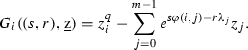
• (ii) Analyticity of . This has been proven in [8, Proposition 4.2] for the case when all $\lambda _i$’s are the same. We adapt the proof given there with minor modifications. We consider the map $G: {\mathbb {R}}^2\times {\mathbb {R}}_+^{m}\rightarrow {\mathbb {R}}^{m}$ defined by

  

  where

  

  It is clear that G is real-analytic. By Lemma 1, for any fixed $(s,r)\in {\mathbb {R}}^2$, is the unique positive vector satisfying

  

  By the Implicit Function Theorem, to prove the analyticity of , we only need to show that the Jacobian matrix

  

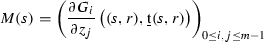
  is invertible for all $(s,r)\in {\mathbb {R}}^2$. To this end, we consider the following matrix

  

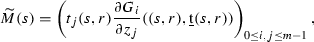
  obtained by multiplying the j-th column of M(s) by $t_j(s,r)$ for each $0\le j\le m-1$. Then $\det (M(s))\ne 0$ if and only if $\det ({\widetilde{M}}(s))\ne 0$. Thus it suffices to prove that ${\widetilde{M}}(s)$ is invertible. We will show that ${\widetilde{M}}(s)$ is strictly diagonal dominating. Then by Gershgorin Circle Theorem (see e.g. [17, Theorem 1.4, page 6]), ${\widetilde{M}}(s)$ is invertible. Recall that a matrix is said to be strictly diagonal dominating if for every row of the matrix, the modulus of the diagonal entry in the row is strictly larger than the sum of the modulus of all the other (non-diagonal) entries in that row. Now we are left to show that for any $0\le i\le m-1$,

  

  (5)

  In fact, we have

  

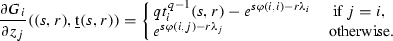
  Then, substituting the last expression into (5), we deduce that the left hand side of (5) is equal to

  $$\begin{aligned} qt_i^{q}(s,r)-\sum _{j=0}^{m-1}e^{s\varphi (i,j)-r\lambda _j}t_j(s,r). \end{aligned}$$

  (6)

  By the fact that is the fixed vector of ${\mathcal {N}}_{(s,r)}$, (6) is equal to $(q-1)t_i^q(s,r)$ which is strictly positive.

• (iii) Convexity of and P(s, r). When all $\lambda _i$’s are the same, the convexity results of and P(s, r) have been proven in detail in Sections 4 and 5 of [8] by studying the operator ${\mathcal {N}}_{(s,r)}$. The main idea there is to prove by induction the convexity of each . Then the limit is also convex. For the strict convexity of , one uses analyticity property and the fact that a convex analytic function is either strictly convex or linear. We will omit the proofs which are elementary and are just minor modifications of those of [8]. One can refer to Sections 4, 5 and also 10 of [8].

$\square$

To end this subsection, we give the following remark on the monotonicity of the function $r\mapsto P(s,r)$.

Remark 1

Observe that for any fixed $s\in {\mathbb {R}}$, the function $r\mapsto {\mathcal {N}}_{(s,r)}^n{\bar{1}}$ is decreasing for all n. Thus for all $0\le i \le m-1$, the function $r\mapsto t_i(s,r)$ is also decreasing, and so is the function $r\mapsto P(s,r)$.

2.2 Construction of telescopic product measures and law of large numbers

An important tool for the study of the multiple ergodic average of $\varphi$, introduced in [11, 12] and used in [5, 8, 14, 15], is the telescopic product measure. This class of measures will also be the main ingredient of our proofs concerning the estimate of Hausdorff dimension of $L_\varphi (\alpha )$. Let us recall the definition of the telescopic product measure. Consider the following partition of ${\mathbb {N}}^*$:

$$\begin{aligned} {\mathbb {N}}^*=\bigsqcup _{i\ge 1,q\not \mid i}\Lambda _i\ \ \mathrm{with}\ \Lambda _i=\{iq^j\}_{j\ge 0}. \end{aligned}$$

Then we decompose $\Sigma _m$ as follows:

$$\begin{aligned} \Sigma _m=\prod _{i\ge 1,q\not \mid i}S^{\Lambda _i}. \end{aligned}$$

Let $\mu$ be a probability measure on $\Sigma _m$. We consider $\mu$ as a measure on $S^{\Lambda _i}$, which is identified with $\Sigma _m$, for every i with $q\not \mid i$. Let $\mu _i$ be a copy of $\mu$ on $S^{\Lambda _i}$ and ${\mathbb {P}}_{\mu }=\prod _{i\le n,q\not \mid i}\mu _i$. More precisely, for any word u of length n we define

$$\begin{aligned} {\mathbb {P}}_{\mu }([u])=\prod _{i\le n,q\not \mid i}\mu ([u_{|_{\Lambda _i}}]), \end{aligned}$$

where [u] denotes the cylinder set of all sequences starting with u and

$$\begin{aligned}u_{|_{\Lambda _i}}=u_iu_{iq}\cdots u_{iq^j}, \quad iq^j\le |u|<iq^{j+1}.\end{aligned}$$

We call ${\mathbb {P}}_{\mu }$ the telescopic product measure associated to $\mu$.

Below, we construct a special class of Markov measures whose initial laws and transition probabilities are determined by the fixed point $(t_i(s,r))_{i\in S}$ of the operator ${\mathcal {N}}_{(s,r)}$. The corresponding telescopic product measure will play a central role in the study of $E_\varphi (\alpha )$.

Recall that $(t_i(s,r))_{i\in S}$ satisfies

$$\begin{aligned} t_i(s,r)^q=\sum _{j=0}^{m-1}e^{s\varphi (i,j)-r\lambda _j}t_j(s,r),\quad (i=0,\ldots ,m-1). \end{aligned}$$

The functions $t_i(s,r)$ allow us to define a Markov measure $\mu _{s,r}$ with initial law $\pi _{s,r}=(\pi (i))_{i\in S}$ and probability transition matrix $Q_{s,r}=(p_{i,j})_{S\times S}$ defined by

$$\begin{aligned} \pi (i) = \frac{t_i(s,r)e^{-r\lambda _i}}{t_0(s,r)e^{r\lambda _0} + \cdots + t_{m-1}(s,r)e^{r\lambda _{m-1}}}, \qquad p_{i, j}= e^{s \varphi (i, j)-r\lambda _j} \frac{t_j(s,r)}{t_i(s,r)^q}. \end{aligned}$$

(7)

We denote by ${\mathbb {P}}_{s,r}$ the telescopic product measure associated to $\mu _{s,r}$. Recall that $\Pi$ is the coding map from $\Sigma _m$ to [0, 1]. Define

$$\begin{aligned}\nu _{s,r}=\Pi _*{\mathbb {P}}_{s,r}={\mathbb {P}}_{s,r}\circ \Pi ^{-1}.\end{aligned}$$

We will use the following law of large numbers which is proved in [8].

Theorem 2

(Theorem 2.6 in [8]) Let $\mu$ be any probability measure on $\Sigma _m$ and let F be a real-valued function defined on $S\times S$. For ${\mathbb {P}}_{\mu }$ a.e. $x\in \Sigma _m$ we have

$$\begin{aligned} \lim _{n\rightarrow \infty }\frac{1}{n}\sum _{k=1}^nF(x_k, x_{kq})=(q-1)^2\sum _{k=1}^\infty \frac{1}{q^{k+1}}\sum _{j=0}^{k-1}{\mathbb {E}}_\mu F(x_j,x_{j+1}). \end{aligned}$$

3 Local dimension of $\nu _{s,r}$

For a Borel measure $\mu$ on a metric space X, the lower local dimension of $\mu$ at a point $x\in X$ is defined by

$$\begin{aligned} {\underline{D}}(\mu ,x):=\liminf _{r\rightarrow 0} \frac{\log \mu (B(x,r))}{\log r}. \end{aligned}$$

If the limit exists, then the limit will be called the local dimension of $\mu$ at x, and denoted by ${D}(\mu ,x)$.

In this section, we study the local dimension of $\nu _{s,r}$. The main results of this section are Propositions 3, 4, and 5. Proposition 3 gives estimates of the local dimensions of $\nu _{s,r}$ on the level set $L_\varphi (\alpha )$. Proposition 4 proves that $\nu _{s,r}$ is supported on $L_\varphi (\frac{\partial P}{\partial s}(s,r))$. In Proposition 5, it is shown that $\nu _{s,r}$ is exact dimensional, i.e., the local dimension of $\nu _{s,r}$ exists and is constant almost surely. The exact formula of this constant is given as well.

We first give an explicit relation between the mass ${\mathbb {P}}_{s,r}([x_1^n])$ and the multiple ergodic sum $\sum _{j=1}^n\varphi (x_j,x_{qj})$. For $x\in \Sigma _m$, define

$$\begin{aligned}B_n(x)=\sum _{j=1}^n \log t_{x_j}(s,r).\end{aligned}$$

Proposition 2

We have

$$\begin{aligned} \log {\mathbb {P}}_{s,r}([x_1^n])=s\sum _{j=1}^{\lfloor \frac{n}{q}\rfloor }\varphi (x_j,x_{jq})-\left( n-\lfloor \frac{n}{q}\rfloor \right) \frac{P(s,r)}{q-1}-r\sum _{j=1}^n\lambda _{x_j}-qB_{\lfloor \frac{n}{q}\rfloor }(x)+B_n(x). \end{aligned}$$

Proof

For $q \not \mid i$, let $\Lambda _i(n)=\Lambda _i\cap [1,n]$. By the definition of ${\mathbb {P}}_{s,r}$, we have

$$\begin{aligned}-\log {\mathbb {P}}_{s,r}[x_1^n]=-\sum _{q\not \mid i,i\le n}\log \mu _{s,r}[x_1^n|_{\Lambda _i(n)}]. \end{aligned}$$

We classify $\Lambda _i(n)$ ($q\not \mid i, i\le n$) according to their length $|\Lambda _i(n)|$. We have $\min _{q\not \mid i, i\le n} |\Lambda _i(n)|=1$ and $\max _{q\not \mid i, i\le n} |\Lambda _i(n)|=\lfloor \log _q n\rfloor$. Observe that $|\Lambda _i(n)|=k$ if and only if $\frac{n}{q^k}<i\le \frac{n}{q^{k-1}}.$ Therefore

$$\begin{aligned} -\log {\mathbb {P}}_{s,r}[x_1^n]=- \sum _{k=1}^{\lfloor \log _q n\rfloor }\sum _{\frac{n}{q^k} <i\le \frac{n}{q^{k-1}}, q\not \mid i}\log \mu _{s,r}[x_1^n|_{\Lambda _i(n)}]. \end{aligned}$$

(8)

Denote $t_\emptyset (s,r):=\sum _{j=0}^{m-1}t_j(s,r)e^{-r\lambda _j}$. For simplicity, we also write $t_\emptyset$ and $t_j$ for $t_\emptyset (s,r)$ and $t_j(s,r)$ and keep their dependences on s and r in mind.

By the definition of $\mu _{s,r}$, for i with $\frac{n}{q^k} <i\le \frac{n}{q^{k-1}}$, we have

$$\begin{aligned} \log \mu _{s,r}[x_1^n|_{\Lambda _i(n)}]&= \log \frac{t_{x_i} e^{-r\lambda _{x_i}}}{t_\emptyset }+\sum _{j=1}^{k-1}\log \left( e^{s\varphi (x_{iq^{j-1}},x_{iq^j})-r\lambda _{x_{iq^j}}}\frac{t_{x_{iq^j}}}{t_{x_{iq^{j-1}}}^q}\right) \\&=s S_{n,i}\varphi (x)-(q-1)S_{n,i}t(x)+\log t_{x_{iq^{k-1}}}-rS_{n,i}\lambda (x)-\log t_\emptyset , \end{aligned}$$

where $S_{n,i}\varphi (x)=\sum _{j=1}^{k-1}\varphi (x_{iq^{j-1}},x_{iq^j})$, $S_{n,i}t(x)=\sum _{j=1}^{k-1}\log t_{x_{iq^{j-1}}}$ and $S_{n,i}\lambda (x)=\sum _{j\in \Lambda _i(n)} \lambda _{x_{j}}$. Substituting the above expressions in (8) and noticing that $\frac{n}{q^k}<i\le \frac{n}{q^{k-1}}$ is equivalent to $\frac{n}{q}<iq^{k-1}\le n$, we obtain

$$\begin{aligned} \log {\mathbb {P}}_{s,r}[x_1^n]= & {} s \sum _{q\not \mid i,i\le n}S_{n,i}\varphi (x)-(q-1)\sum _{q\not \mid i,i\le n}S_{n,i}t(x) +\sum _{\frac{n}{q} \le \ell <n}\log t_{x_\ell }\\&-r \sum _{q\not \mid i,i\le n}S_{n,i}\lambda (x)-\sharp \{q\not \mid i,i\le n\}\log t_\emptyset \\= & {} s \sum _{j=1}^{\lfloor \frac{n}{q}\rfloor }\varphi (x_j,x_{jq})-(q-1)\sum _{j=1}^{\lfloor \frac{n}{q}\rfloor } \log t_{x_j}+\sum _{\ell =\lfloor \frac{n}{q}\rfloor +1}^n\log t_{x_\ell }\\&-r\sum _{j=1}^n\lambda _{x_j}-\left( n-\lfloor \frac{n}{q}\rfloor \right) \log t_\emptyset . \end{aligned}$$

We then end the proof by observing that $(q-1)\log t_\emptyset (s,r)=P(s,r)$ and

$$\begin{aligned}-(q-1)\sum _{j=1}^{\lfloor \frac{n}{q}\rfloor } \log t_{x_j} +\sum _{\ell =\lfloor \frac{n}{q}\rfloor +1}^n\log t_{x_\ell }=-qB_{\lfloor \frac{n}{q}\rfloor }(x)+B_n(x).\end{aligned}$$

$\square$

3.1 Local dimensions of $\nu _{s,r}$ on level sets

As an application of Proposition 2, we obtain an upper bound for the local dimension of $\nu _{s,r}$ on $L_\varphi (\alpha )$ in Proposition 3 below. The following elementary result will be useful for the estimates of local dimension of $\nu _{s,r}$.

Lemma 2

Let $(a_n)_{n\ge 1}$ be a bounded sequence of non-negative real numbers. Then

$$\begin{aligned}\liminf _{n\rightarrow \infty }\left( a_{\lfloor \frac{n}{q} \rfloor }-a_n\right) \le 0.\end{aligned}$$

Proof

Let $b_l=a_{q^{l-1}}-a_{q^{l}}$ for $l\in {\mathbb {N}}^*$. Then the boundedness implies

$$\begin{aligned}\lim _{l \rightarrow \infty }\frac{b_1+\cdots +b_l}{l}= \lim _{l \rightarrow \infty } \frac{a_1-a_{q^l}}{l}=0.\end{aligned}$$

This in turn implies $\liminf _{l\rightarrow \infty }b_l\le 0$. Thus

$$\begin{aligned}\liminf _{l\rightarrow \infty }\left( a_{\lfloor \frac{n}{q} \rfloor }-a_n\right) \le \liminf _{l\rightarrow \infty }b_l\le 0.\end{aligned}$$

$\square$

Proposition 3

For any $x\in E_\varphi (\alpha )$, we have

$$\begin{aligned}\liminf _n\frac{\log \nu _{s,r}(\Pi [x_1^n])}{\log |\Pi [x_1^n]|}\le r+\limsup _n\frac{P(s,r)/q-\alpha s/q }{(\sum _{j=1}^n\lambda _{x_j})/n}.\end{aligned}$$

Proof

Since $\nu _{s,r}(\Pi [x_1^n])={\mathbb {P}}_{s,r}([x_1^n])$, by Proposition 2 we can write $\log \nu _{s,r}(\Pi [x_1^n])$ as

$$\begin{aligned} s\sum _{j=1}^{\lfloor \frac{n}{q}\rfloor }\varphi (x_j,x_{jq})-(n-\lfloor \frac{n}{q}\rfloor )\frac{P(s,r)}{q-1}-r\sum _{j=1}^n\lambda _{x_j}-qB_{\lfloor \frac{n}{q}\rfloor }(x)+B_n(x).\end{aligned}$$

On the other hand, $\log |\Pi [x_1^n]|=-\sum _{j=1}^n\lambda _{x_j}$. Thus, for $x\in E_\varphi (\alpha )$

$$\begin{aligned}&\liminf _n\frac{\log \nu _{s,r}(\Pi [x_1^n])}{\log |\Pi [x_1^n]|}\\&\quad \le \limsup _n\frac{P(s,r)/q-\alpha s/q }{(\sum _{j=1}^n\lambda _{x_j})/n}+r+\liminf _n\frac{\frac{q}{n}B_{\lfloor \frac{n}{q}\rfloor }(x)-\frac{1}{n}B_n(x)}{(\sum _{j=1}^n\lambda _{x_j})/n}. \end{aligned}$$

Then, we end the proof by applying Lemma 2 to the sequence $\frac{1}{n}B_n(x)$:

$$\begin{aligned}\liminf _n \left( \frac{q}{n}B_{\lfloor \frac{n}{q}\rfloor }(x)-\frac{1}{n}B_n(x)\right) \le 0.\end{aligned}$$

$\square$

Remark 2

Denote $\lambda _{\min }=\min _i\lambda _i$ and $\lambda _{\max }=\max _i\lambda _i$. Let

$$\begin{aligned}{\widetilde{\lambda }}(x):= \liminf _{n\rightarrow \infty } \frac{1}{n}\sum _{j=1}^n\lambda _{x_j}.\end{aligned}$$

Then ${\widetilde{\lambda }}(x)\in [\lambda _{\min },\lambda _{\max }]$ and

$$\begin{aligned} \limsup _n\frac{P(s,r)/q-\alpha s/q }{(\sum _{j=1}^n\lambda _{x_j})/n}&=\frac{P(s,r)/q-\alpha s/q }{{\widetilde{\lambda }}(x)}. \end{aligned}$$

Hence we deduce from Proposition 3 that for any $x\in L_\varphi (\alpha )$

$$\begin{aligned} {\underline{D}}(\nu _{s,r},x)\le r+\frac{P(s,r)/q-\alpha s/q }{{\widetilde{\lambda }}(x)}, \ (s,r)\in {\mathbb {R}}^2. \end{aligned}$$

(9)

We have estimated the local dimension of $\nu _{s,r}$ on the level set $L_\varphi (\alpha )$. In the following proposition we show that $\nu _{s,r}$ is supported on $L_\varphi (\frac{\partial P}{\partial s}(s,r))$.

Proposition 4

For ${\mathbb {P}}_{s,r}$-a.e. $x=(x_i)_{i=1}^\infty \in \Sigma _m$, we have

$$\begin{aligned} \lim _{n\rightarrow \infty }\frac{1}{n}\sum _{k=1}^n\varphi (x_k,x_{kq})=\frac{\partial P}{\partial s}(s,r). \end{aligned}$$

(10)

In particular, $\nu _{s,r}(L_\varphi (\frac{\partial P}{\partial s}(s,r)))=1$.

Proof

We first prove the statement (10). By Theorem  2, we have for ${\mathbb {P}}_{s,r}$-a.e. $x\in \Sigma _m$

$$\begin{aligned} \lim _{n\rightarrow \infty }\frac{1}{n}\sum _{k=1}^n\varphi (x_k,x_{kq})=(q-1)^2\sum _{k=1}^\infty \frac{1}{q^{k+1}}\sum _{h=0}^{k-1}{\mathbb {E}}_{\mu _{s,r}} \varphi (x_h,x_{h+1}). \end{aligned}$$

(11)

Thus we only need to prove that the right hand side of (11) equals to $\frac{\partial P}{\partial s}(s,r)$. Observe that ${\mathbb {E}}_{\mu _{s,r}} \varphi (x_h,x_{h+1})$ can be expressed as

with

$$\begin{aligned} \pi =\left( \frac{t_i(s,r)e^{-r\lambda _i}}{t_\emptyset (s,r)}\right) _{i\in S}, \qquad Q= \left( e^{s \varphi (i, j)-r\lambda _j} \frac{t_j(s,r)}{t_i(s,r)^q}\right) _{(i,j)\in S\times S}\end{aligned}$$

and

$$\begin{aligned}{\widetilde{Q}}=\left( e^{s\varphi (i,j)-r\lambda _j}\varphi (i,j)\frac{t_j(s,r)}{t_i^q(s,r)}\right) _{(i,j)\in S\times S}.\end{aligned}$$

Recall that $(t_i(s,r))_i$ is the fixed point of ${\mathcal {N}}_{s,r}$:

$$\begin{aligned} t_i^q(s,r)=\sum _{j=0}^{m-1}e^{s\varphi (i,j)-r\lambda _j}t_j(s,r),\quad (i,j)\in S\times S. \end{aligned}$$

(12)

Taking the derivative with respect to s of both sides of (12), we get

$$\begin{aligned}qt_i^{q-1}(s)\frac{\partial t_i}{\partial s}(s,r)=\sum _{j=0}^{m-1}\left( e^{s\varphi (i,j)-r\lambda _j}\varphi (i,j)t_j(s,r)+ e^{s\varphi (i,j)}\frac{\partial t_j}{\partial s}(s,r)\right) .\end{aligned}$$

Dividing both sides of the above equation by $t^q_i(s,r)$, we obtain

$$\begin{aligned} \sum _{j=0}^{m-1}e^{s\varphi (i,j)-r\lambda _j}\varphi (i,j)\frac{t_j(s,r)}{t_i^q(s,r)}=q\frac{\frac{\partial t_i}{\partial s}(s,r)}{t_i(s,r)}- \sum _{j=0}^{m-1}e^{s\varphi (i,j)} \frac{\frac{\partial t_j}{\partial s}(s,r)}{t_i^q(s,r)}. \end{aligned}$$

(13)

Let w and v be two vectors defined by

$$\begin{aligned}w=q\left( \frac{\frac{\partial t_0}{\partial s}(s,r)}{t_0(s)}, \dots , \frac{\frac{\partial t_{m-1}}{\partial s}(s,r)}{t_{m-1}(s)}\right) ^t\end{aligned}$$

and

$$\begin{aligned}v=\left( \sum _{j=0}^{m-1}e^{s\varphi (0,j)} \frac{\frac{\partial t_j}{\partial s}(s,r)}{t_0^q(s)}, \dots , \sum _{j=0}^{m-1}e^{s\varphi (m-1,j)} \frac{\frac{\partial t_j}{\partial s}(s,r)}{t_{m-1}^q(s)}\right) .\end{aligned}$$

Then, by (13), we have

Observe that $Qw=qv$, therefore

(14)

where we denote $S_k=\sum _{h=0}^{k-1}\pi Q^{h}v$ for $k\ge 1$ and $S_{0}=0$. Denote by $\alpha (s)$ the right hand side of (11). Observe that $S_k/q^k\rightarrow 0$ when $k\rightarrow \infty$. Substituting (14) in (11), we obtain

$$\begin{aligned} \alpha (s)&= (q-1)^2\sum _{k=1}^\infty \frac{1}{q^{k+1}} \left( \pi w+ qS_{k-1}- S_k\right) \\&=(q-1)^2\sum _{k=1}^\infty \frac{1}{q^{k+1}}\pi w \\ {}&= \frac{q-1}{q}\pi w =(q-1)\frac{\sum _{j=0}^{m-1}\frac{\partial t_j}{\partial s}(s,r)e^{-r\lambda _j}}{t_\emptyset (s,r)}= \frac{\partial P}{\partial s}(s,r). \end{aligned}$$

Now we show that $\nu _{s,r}(L_\varphi (\frac{\partial P}{\partial s}(s,r)))=1$. Since (10) holds for ${\mathbb {P}}_{s,r}$ a.e. x we have

$$\begin{aligned}{\mathbb {P}}_{s,r}\left( E_\varphi \left( \frac{\partial P}{\partial s}(s,r)\right) \right) =1.\end{aligned}$$

Hence

$$\begin{aligned} \nu _{s,r}\left( L_\varphi \Big (\frac{\partial P}{\partial s}(s,r)\Big )\right)&={\mathbb {P}}_{s,r}\left( \Pi ^{-1}\Big (L_\varphi \big (\frac{\partial P}{\partial s}(s,r)\big )\Big )\right) \\&={\mathbb {P}}_{s,r}\left( E_\varphi \Big (\frac{\partial P}{\partial s}(s,r)\Big )\right) =1. \end{aligned}$$

$\square$

Let $\lambda (s,r)$ be the expected limit with respect to ${\mathbb {P}}_{s,r}$ of the average of the Lyapunov exponents $\frac{1}{n}\sum _{k=1}^n\lambda _{\omega _k}$ with $\omega \in \Sigma _m$. By Theorem 2, we have

$$\begin{aligned}\lambda (s,r)=(q-1)^2\sum _{k=1}^\infty \frac{1}{q^{k+1}}\sum _{j=0}^{k-1}{\mathbb {E}}_{\mu _{s,r}} \lambda _{\omega _j}.\end{aligned}$$

As an application of Proposition 4, we show that the measure $\nu _{s,r}$ is exact dimensional and we have the following formula for its dimension.

Proposition 5

For $\nu _{s,r}$-a.e. x we have

$$\begin{aligned}D(\nu _{s,r},x)=r+\frac{P(s,r)-s\frac{\partial P}{\partial s}(s,r)}{q\lambda (s,r)}.\end{aligned}$$

Proof

We only need to show that for ${\mathbb {P}}_{s,r}$-a.e. $y\in \Sigma _m$

$$\begin{aligned} \lim _{n\rightarrow \infty } \frac{\log {\mathbb {P}}_{s,r}([y_1^n])}{\log |\Pi ([y_1^n])|}=r+\frac{P(s,r)-s\frac{\partial P}{\partial s}(s,r)}{q\lambda (s,r)}. \end{aligned}$$

(15)

Since $|\Pi ([y_1^n])|=e^{-\sum _{k=1}^n\lambda _{y_k}}$, from the discussion preceding Proposition 5, we get for ${\mathbb {P}}_{s,r}$-a.e. y

$$\begin{aligned} \lim _{n\rightarrow \infty } \frac{\log |\Pi ([y_1^n])|}{n}=-\lambda (s,r). \end{aligned}$$

(16)

On the other hand, by Theorem 2, Propositions 2 and 4, we have for ${\mathbb {P}}_{s,r}$-a.e. y

$$\begin{aligned} \lim _{n\rightarrow \infty } \frac{\log {\mathbb {P}}_{s,r}([y_1^n])}{n}= \frac{s}{q}\frac{\partial P}{\partial s}(s,r)-\frac{1}{q}P(s,r)-r\lambda (s,r). \end{aligned}$$

(17)

Combining (16) and (17), we get (15).

$\square$

4 Further properties of the pressure function and study of the system (4)

The main result of this section is Proposition 6 below on the solution of the system (4).

We will use the following lemma concerning the range of the partial derivatives of P(s, r). Recall the definition (3).

Lemma 3

For any $r\in {\mathbb {R}}$, we have

$$\begin{aligned}\left\{ \frac{\partial P}{\partial s}(s,r) : s\in {\mathbb {R}}\right\} =(A,B)\end{aligned}$$

Proof

Fix $r_0\in {\mathbb {R}}$. Since $s\mapsto P(s,r)$ is convex, It suffices to show that

$$\begin{aligned}\lim _{s\rightarrow +\infty }\frac{\partial P}{\partial s}(s,r_0) =B \quad \text {and}\quad \lim _{s\rightarrow -\infty }\frac{\partial P}{\partial s}(s,r_0) =A.\end{aligned}$$

We only give the proof for the case when s goes to $+\infty$. The case for s tending to $-\infty$ is similar. The proof will be done by contradiction. Suppose that there exists $\epsilon >0$ such that

$$\begin{aligned}\frac{\partial P}{\partial s}(s,r_0) \le B-\epsilon \quad \text {for all }\ s\in {\mathbb {R}}.\end{aligned}$$

By the Mean Value Theorem, for any $s>0$, we have

$$\begin{aligned} P(s,r_0)-P(0,r_0)\le s(B-\epsilon ). \end{aligned}$$

(18)

By the definition of B, there exists $(s',r')\in {\mathbb {R}}^2$ such that $\frac{\partial P}{\partial s}(s',r')=B-\epsilon /2$. By Proposition 4, $\nu _{s',r'}(L_\varphi (B-\epsilon /2))=1$, so $L_\varphi (B-\epsilon /2)\ne \emptyset .$ Let $x\in L_\varphi (B-\epsilon /2)$. By Proposition 3 and Remark 2, we have

$$\begin{aligned}{\underline{D}}(\nu _{s,r_0},x)\le r_0+\frac{P(s,r_0)/q-(B-\epsilon /2) s/q }{{\widetilde{\lambda }}(x)}.\end{aligned}$$

Substituting (18) in the above inequality, we get

$$\begin{aligned}{\underline{D}}(\nu _{s,r_0},x)\le r_0+\frac{P(0,r_0)/q-\epsilon s/2q }{{\widetilde{\lambda }}(x)}. \end{aligned}$$

Since ${\widetilde{\lambda }}(x)\in [\lambda _{\min },\lambda _{\max }]\subset (0,+\infty )$, the second term in the right hand side of the above inequality tends to $-\infty$ when $s\rightarrow +\infty$. Hence, for s large enough we must have ${\underline{D}}(\nu _{s,r_0},x)<0$. But this is impossible since $\nu _{s,r_0}$ is a probability measure. Thus, we conclude that $\lim _{s\rightarrow +\infty }\frac{\partial P}{\partial s}(s,r_0) =B$.

$\square$

Proposition 6

For any $\alpha \in (A,B)$, there exists a unique solution $(s(\alpha ),r(\alpha ))\in {\mathbb {R}}^2$ to the system

$$\begin{aligned} \left\{ \begin{array}{ll} P(s,r)&{}=\alpha s\\ \frac{\partial P}{\partial s}(s,r)&{}=\alpha , \end{array} \right. \end{aligned}$$

(19)

Moreover the functions $s(\alpha ), r(\alpha )$ are analytic on (A, B).

Proof

• (1) Existence and uniqueness of the solution $(s(\alpha ),r(\alpha ))$. Fix $\alpha \in (A,B)$. By Lemma 3 and the strict convexity of $s\mapsto P(s,r)$, for any $r\in {\mathbb {R}}$, there exists a unique $s=s(\alpha ,r)\in {\mathbb {R}}$ such that

  $$\begin{aligned} \frac{\partial P}{\partial s}(s(\alpha ,r),r)=\alpha . \end{aligned}$$

  (20)

  In the following, we will show that there exists a unique solution $r=r(\alpha )\in {\mathbb {R}}$ to the equation

  $$\begin{aligned}P(s(\alpha ,r),r)=\alpha s(\alpha ,r).\end{aligned}$$

  Set $h(r):=P(s(\alpha ,r),r)-\alpha s(\alpha ,r)$. By (20)

  $$\begin{aligned} h'(r)= & {} \frac{\partial P}{\partial s}(s(\alpha ,r),r)\frac{\partial s(\alpha ,r)}{\partial r}+\frac{\partial P}{\partial r}(s(\alpha ,r),r)-\alpha \frac{\partial s(\alpha ,r)}{\partial r}\\= & {} \frac{\partial P}{\partial r}(s(\alpha ,r),r). \end{aligned}$$

  Note that we can take the partial derivative of s with respect to r by the implicit function theorem. For fixed s the function $r\mapsto P(s,r)$ is strictly decreasing, since it is strictly convex and decreasing (Remark 1). Hence $\frac{\partial P}{\partial r}(s(\alpha ,r),r) <0$ and thus h(r) is also strictly decreasing. For the rest of the proof, we only need to show $\lim _{r\rightarrow +\infty } h(r)<0$ and $\lim _{r\rightarrow -\infty } h(r)>0$, then we conclude by applying the Intermediate Value Theorem. By Proposition 5, we have

  $$\begin{aligned}\dim \nu _{s(\alpha ,r),r} =r+\frac{P(s(\alpha ,r),r)-s(\alpha ,r)\alpha }{q\lambda (s(\alpha ,r),r)}.\end{aligned}$$

  Observe that for any $r\in {\mathbb {R}}$, we have always $0\le \dim \nu _{s(\alpha ,r),r}\le 1$ and $0<\lambda _{\min }\le \lambda (s(\alpha ,r),r)\le \lambda _{\max }$. Therefore we have

  $$\begin{aligned}\lim _{r\rightarrow +\infty }h(r)=\lim _{r\rightarrow +\infty }\left( \dim \nu _{s(\alpha ,r),r} -r\right) q\lambda (s(\alpha ,r),r)<0.\end{aligned}$$

  Similarly,

  $$\begin{aligned}\lim _{r\rightarrow -\infty }h(r)>0.\end{aligned}$$

• (2) Analyticity of $(s(\alpha ),r(\alpha ))$. Consider the map

  $$\begin{aligned}F = \left( \begin{array}{ccc} F_1 \\ F_2 \end{array} \right) = \left( \begin{array}{ccc} P(s,r)- \alpha s\\ \frac{\partial P}{\partial s}(s,r)-\alpha \end{array} \right) . \end{aligned}$$

  The jacobian matrix of F is equal to

  $$\begin{aligned} J(F) := \left( \begin{array}{ccc} \frac{\partial F_1}{\partial s} &{} \frac{\partial F_1}{\partial r} \\ \frac{\partial F_2}{\partial s} &{} \frac{\partial F_2}{\partial r} \end{array} \right) = \left( \begin{array}{ccc} \frac{\partial P}{\partial s}-\alpha &{} \frac{\partial P}{\partial r}\\ \frac{\partial ^2 P}{\partial s^2} &{} \frac{\partial ^2 P}{\partial r \partial s } \end{array} \right) . \end{aligned}$$

  Thus we have

  $$\begin{aligned}\det (J(F))|_{s=s(\alpha ),r=r(\alpha )}=-\frac{\partial ^2 P}{\partial s^2}\cdot \frac{\partial P}{\partial r}\ne 0.\end{aligned}$$

  Then by the Implicit Function Theorem, $s(\alpha )$ and $r(\alpha )$ are analytic.

$\square$

5 Proof of Theorem 1

5.1 Computation of $\dim _H L_\varphi (\alpha )$ for $\alpha \in (A,B)$

We will use the following Billingsley Lemma.

Lemma 4

(see e.g. Proposition 4.9. in [3]) Let $E\subset \Sigma _m$ be a Borel set and let $\mu$ be a finite Borel measure on $\Sigma _m$.

• (i) If $\mu (E) > 0$ and ${\underline{D}}(\mu ,x)\ge d$ for $\mu$-a.e x, then $\dim _H(E)\ge d$;

• (ii) If ${\underline{D}}(\mu ,x)\le d$ for all $x \in E$, then $\dim _H(E) \le d$.

Theorem 3

For any $\alpha \in (A,B)$, we have

$$\begin{aligned} \dim _HL_\varphi (\alpha )=r(\alpha ). \end{aligned}$$

Proof

By (9) and the equality $P(s(\alpha ),r(\alpha ))=\alpha s(\alpha )$, we have

$$\begin{aligned} {\underline{D}}(\nu _{s(\alpha ),r(\alpha )},x)\le r(\alpha ) \ \text { for all }\ x\in L_\varphi (\alpha ). \end{aligned}$$

Then Lemma 4 implies that

$$\begin{aligned} \dim _HL_\varphi (\alpha )\le r(\alpha ). \end{aligned}$$

By Proposition 4 and the equality $\frac{\partial P}{\partial s}(s(\alpha ),r(\alpha ))=\alpha$, we know that

$$\begin{aligned} \nu _{s(\alpha ),r(\alpha )}(L_\varphi (\alpha ))=1. \end{aligned}$$

On the other hand, by Proposition 5,

$$\begin{aligned} D(\nu _{s(\alpha ),r(\alpha )},x)= r(\alpha ) \quad \text { for }\ \nu _{s(\alpha ),r(\alpha )}\mathrm{-a.e.} \ x. \end{aligned}$$

Applying Lemma 4 again, we obtain

$$\begin{aligned} \dim _HL_\varphi (\alpha )\ge r(\alpha ). \end{aligned}$$

$\square$

5.2 Range of $\{\alpha : L_\varphi (\alpha )\ne \emptyset \}$

Proposition 7

We have $\{\alpha : L_\varphi (\alpha )\ne \emptyset \}\subset [A,B].$

Proof

We prove it by contradiction. Suppose that $L_\varphi (\alpha )\ne \emptyset$ for some $\alpha >B$. Let $x\in L_\varphi (\alpha )$. Then by (9) and taking $r=0$, we have

$$\begin{aligned} {\underline{D}}(\nu _{s,0},x)\le \frac{P(s,0)-\alpha s }{q{\widetilde{\lambda }}(x)} \quad \text { for all } s\in {\mathbb {R}}. \end{aligned}$$

(21)

On the other hand, by the mean value theorem, we have

$$\begin{aligned} P(s,0)-\alpha s=\frac{\partial P}{\partial s}(\eta _s,0)s-\alpha s+P(0,0) \end{aligned}$$

(22)

for some real number $\eta _s$ between 0 and s. In the following, we suppose that $s>0$. Substituting (22) in (21), we get

$$\begin{aligned}{\underline{D}}(\nu _{s,0},x)\le \frac{\frac{\partial P}{\partial s}(\eta _s,0)s-\alpha s+P(0,0)}{q{\widetilde{\lambda }}(x)}\le \frac{(B -\alpha ) s+P(0,0)}{q{\widetilde{\lambda }}(x)}.\end{aligned}$$

Since $B-\alpha <0$ and ${\widetilde{\lambda }}(x)\in [\lambda _{\min },\lambda _{\max }]\subset (0,+\infty )$, the last term in the above inequalities tends to $-\infty$ when $s\rightarrow +\infty$. But this is impossible since we have always ${\underline{D}}(\nu _{s,0},x)\ge 0$. Thus we must have $L_\varphi (\alpha )= \emptyset$ for any $\alpha >B$. Similarly we can also prove that $L_\varphi (\alpha )= \emptyset$ for any $\alpha <A$. $\square$

As we will show, we actually have the equality $\{\alpha : L_\varphi (\alpha )\ne \emptyset \}= [A,B]$ (see Theorem 4).

5.3 Computation of $\dim _H L_\varphi (A)$ and $\dim _H L_\varphi (B)$

Now, we consider the level set $L_\varphi (\alpha )$ when $\alpha =A$ or B. The aim of this subsection is to prove the following theorem.

Theorem 4

• (i) The following limits exist:

  $$\begin{aligned}r(A):=\lim _{\alpha \rightarrow A}r(\alpha ),\ \ r(B):=\lim _{\alpha \rightarrow B}r(\alpha ).\end{aligned}$$

• (ii) If $\alpha =A$ or B, then $L_\varphi (\alpha )\ne \emptyset$ and

  $$\begin{aligned}\dim _H L_\varphi (\alpha )=r(\alpha ).\end{aligned}$$

We will give the proof of Theorem 4 for the case $\alpha =A$, the proof for $\alpha =B$ is similar.

5.3.1 Accumulation points of $\mu _{s(\alpha ),r(\alpha )}$ when $\alpha$ tends to A.

As all components of the vector $\pi _{s,r}$ and the matrix $Q_{s,r}$ (see formula (7)) are non-negative and bounded by 1, the set $\{(\pi _{s(\alpha ),r(\alpha )},Q_{s(\alpha ),r(\alpha )}), \alpha \in (A,B)\}$ is precompact. Thus there exists a sequence $(\alpha _n)_n\in (A,B)$ with $\lim _n\alpha _n=A$ such that the limits

$$\begin{aligned} \lim _{n\rightarrow \infty }\pi _{s(\alpha _n),r(\alpha _n)}, \ \ \lim _{n\rightarrow \infty } Q_{s(\alpha _n),r(\alpha _n)} \end{aligned}$$

exist. Using these limits as initial law and transition probability, we construct a Markov measure which we denote by $\mu _\infty$. It is clear that the Markov measure $\mu _{s(\alpha _n),r(\alpha _n)}$ corresponding to $\pi _{s(\alpha _n),r(\alpha _n)}$ and $Q_{s(\alpha _n),r(\alpha _n)}$ converges to $\mu _\infty$ with respect to the weak-star topology. We denote by ${\mathbb {P}}_\infty$ the telescopic product measure associated to $\mu _\infty$ and set $\nu _\infty :={\mathbb {P}}_\infty \circ \Pi ^{-1}$.

Proposition 8

We have

$$\begin{aligned} \nu _\infty (L_\varphi (A))=1. \end{aligned}$$

In particular, $L_\varphi (A)\ne \emptyset$.

Proof

Since $\nu _{\infty }(L_\varphi (A))={\mathbb {P}}_\infty (E_\varphi (A))$, we only need to show that ${\mathbb {P}}_\infty (E_\varphi (A))=1$, i.e., for ${\mathbb {P}}_{\infty }$-a.e. $x\in \Sigma _m$ we have

$$\begin{aligned} \lim _{n\rightarrow \infty }\frac{1}{n}\sum _{k=1}^n\varphi (x_k,x_{kq})=A. \end{aligned}$$

By Theorem 2, for ${\mathbb {P}}_{\infty }$-a.e. $x\in \Sigma _m$ the limit in the left hand side of the above equation equals $M(\mu _\infty )$ where M is the functional on the space of probability measures defined by

$$\begin{aligned} M(\nu )=(q-1)^2\sum _{k=1}^\infty \frac{1}{q^{k+1}}\sum _{j=0}^{k-1}{\mathbb {E}}_\nu \varphi (x_j,x_{j+1}). \end{aligned}$$

The function $\nu \mapsto M(\nu )$ is continuous, since the above series converges uniformly on $\nu$ and the function $\nu \mapsto {\mathbb {E}}_\nu \varphi (x_j,x_{j+1})$ is continuous for all j. Since $\mu _{s(\alpha _n),r(\alpha _n)}$ converges to $\mu _{\infty }$ when $n\rightarrow \infty$, we have that

$$\begin{aligned}\lim _{n\rightarrow \infty }M(\mu _{s(\alpha _n),r(\alpha _n)})=M(\mu _{\infty }). \end{aligned}$$

Recall that the vector $(s(\alpha ),r(\alpha ))$ satisfies $\frac{\partial P}{\partial s}(s(\alpha ),r(\alpha ))=\alpha$. By Proposition 4, we know that

$$\begin{aligned} M(\mu _{s(\alpha _n),r(\alpha _n)})=\alpha _n. \end{aligned}$$

Thus

$$\begin{aligned}M(\mu _{\infty })=\lim _{n\rightarrow \infty }\alpha _n=A.\end{aligned}$$

$\square$

From Theorem 3, we know that for each $\alpha \in (A,B)$, $r(\alpha )=\dim _HL_\varphi (\alpha )\in [0,1]$. Hence, in particular the set $\{r(\alpha ): \alpha \in (A,B)\}$ is bounded.

We have the following formula for $\dim _H \nu _{\infty }$.

Proposition 9

The limit $r(A):=\lim _nr(\alpha _n)$ exists and we have

$$\begin{aligned} \dim \nu _\infty =r(A). \end{aligned}$$

Proof

Let $(\alpha _{n_k})_k$ be any subsequence of $(\alpha _n)_n$ such that the limit $\lim _kr(\alpha _{n_k})$ exists. We will show that this limit is equal to $\dim \nu _\infty$.

We first claim that the measure $\nu _\infty$ is exact dimensional and its dimension is given by

$$\begin{aligned} \dim \nu _\infty =\frac{\dim ({\mathbb {P}}_\infty )}{\lambda ({\mathbb {P}}_\infty )}, \end{aligned}$$

where $\dim ({\mathbb {P}}_\infty )$ is the a.e. local dimension of ${\mathbb {P}}_\infty$ and $\lambda ({\mathbb {P}}_\infty )$ is the expected limit with respect to ${\mathbb {P}}_{\infty }$ of the average of the Lyapunov exponents $\frac{1}{n}\sum _{k=1}^n\lambda _{\omega _k}$ with $\omega \in \Sigma _m$, i.e.,

$$\begin{aligned} \lambda ({\mathbb {P}}_{\infty })=(q-1)^2\sum _{k=1}^\infty \frac{1}{q^{k+1}}\sum _{j=0}^{k-1}{\mathbb {E}}_{\mu _{\infty }} \lambda _{\omega _j}. \end{aligned}$$

To prove the claim, we only need to show that for ${\mathbb {P}}_\infty$-a.e. x

$$\begin{aligned} \lim _{n\rightarrow \infty }\frac{\log \nu _{\infty }(\Pi [x_1^n])}{\log |\Pi [x_1^n]|}=\frac{\dim ({\mathbb {P}}_\infty )}{\lambda ({\mathbb {P}}_\infty )}. \end{aligned}$$

This is proved by using the facts $\nu _{\infty }(\Pi [x_1^n])={\mathbb {P}}_\infty ([x_1^n])$, $\log |\Pi [x_1^n]|=-\sum _{j=1}^n\lambda _{x_j}$ and applying Theorem 2.

By similar arguments as used in the proof of Proposition 8, we can show that the functions

$$\begin{aligned} \mu \mapsto \dim ({\mathbb {P}}_\mu ), \ \ \mu \mapsto \lambda ({\mathbb {P}}_\mu ) \end{aligned}$$

are continuous on the space of probability measures. Thus, we deduce that

$$\begin{aligned} \dim \nu _\infty =\lim _{k\rightarrow \infty }\frac{\dim ({\mathbb {P}}_{\mu _{s(\alpha _{n_k}),r(\alpha _{n_k})}})}{\lambda ({\mathbb {P}}_{\mu _{s(\alpha _{n_k}),r(\alpha _{n_k})}})}=\lim _{k\rightarrow \infty }\dim \nu _{s(\alpha _{n_k}),r(\alpha _{n_k})} =\lim _{k\rightarrow \infty }r(\alpha _{n_k}), \end{aligned}$$

where we have used Theorem 3 for the last equality. Since the subsequence $(\alpha _{n_k})_k$ is arbitrary, we deduce that the limit $r(A):=\lim _nr(\alpha _n)$ exists and $\dim \nu _\infty =r(A)$. $\square$

In the proof of Theorem 4, we will use the following lemma. Recall that for $\alpha \in (A,B)$, the vector $(s(\alpha ),r(\alpha ))$ is the unique solution of the Eq. (19).

Lemma 5

There exists $A'\in (A,B)$ such that

$$\begin{aligned}s(\alpha )<0 \quad \mathrm{for }\ \ \alpha \in (A, A').\end{aligned}$$

Proof

Let

$$\begin{aligned}D:=\left\{ \frac{\partial P}{\partial s}(0,r): r\in [0,1]\right\} .\end{aligned}$$

Then D is a compact subset of ${\mathbb {R}}$. Since for any $r\in {\mathbb {R}}$ the function $s\mapsto \frac{\partial P}{\partial s}(s,r)$ is strictly increasing and $\inf _{s\in {\mathbb {R}}}\frac{\partial P}{\partial s}(s,r)=A$ (Lemma 3), we get $\frac{\partial P}{\partial s}(0,r)>A$ for all $r\in {\mathbb {R}}$. Thus we have $A':=\min \{D\}>A$. Now, we consider the following subset of D:

$$\begin{aligned}D':=\left\{ \frac{\partial P}{\partial s}(0,r(\alpha )): \alpha \in (A,B)\right\} .\end{aligned}$$

We have $\inf D'\ge A'>A$. For any $\alpha <A'$, we have

$$\begin{aligned}\frac{\partial P}{\partial s}(s(\alpha ),r(\alpha ))=\alpha <A'\le \frac{\partial P}{\partial s}(0,r(\alpha )).\end{aligned}$$

Using again the fact that the function $s\mapsto \frac{\partial P}{\partial s}(s,r)$ is strictly increasing, we get

$$\begin{aligned}s(\alpha )<0 \ \ \mathrm{for}\ \ \alpha \in (A,A').\end{aligned}$$

$\square$

Now, we can give the proof of Theorem 4.

Proof of Theorem 4

• (i) Fix any sequence $(\beta _n)_n\in (A,B)$ with $\lim _n\beta _n=A$. Then there exists a subsequence $(\beta _{n_k})_k$ of $(\beta _n)_n$ such that the limits

  $$\begin{aligned}\lim _{k\rightarrow \infty }\pi _{s(\beta _{n_k}),r(\beta _{n_k})}, \ \ \lim _{k\rightarrow \infty } Q_{s(\beta _{n_k}),r(\beta _{n_k})}\end{aligned}$$

  exist. Arguing as in the proof of Proposition 9, we can show that the limit $\lim _kr(\beta _{n_k})$ exists and equals to $\dim \nu _\infty$. Thus, we deduce that the limit $\lim _{\alpha \rightarrow A}r(\alpha )$ exists and equals to $\dim \nu _\infty$.

• (ii) We will show that

  $$\begin{aligned}\dim _H L_\varphi (A)=r(A).\end{aligned}$$

By Propositions 8 and 9 and Lemma 4, we get

$$\begin{aligned}\dim _H L_\varphi (A)\ge r(A).\end{aligned}$$

We now show the reverse inequality. By (9) and Lemma 4 again, we obtain

$$\begin{aligned}\dim _HL_\varphi (A)\le r+\frac{P(s,r)-A s }{q{\widetilde{\lambda }}(x)} \ \ \mathrm{for\ any}\ (s,r)\in {\mathbb {R}}^2.\end{aligned}$$

Note that ${\widetilde{\lambda }}(x)\in [\lambda _{\min },\lambda _{\max }]\subset (0,+\infty )$, and hence ${\widetilde{\lambda }}(x)>0$. For any $\alpha \in (A,A')$, we have

$$\begin{aligned}P(s(\alpha ),r(\alpha ))-As(\alpha )=P(s(\alpha ),r(\alpha ))-\alpha s(\alpha )+(\alpha -A)s(\alpha )=(\alpha -A)s(\alpha )<0,\end{aligned}$$

where for the second equality we have used the fact that $P(s(\alpha ),r(\alpha ))=\alpha s(\alpha )$ and the last inequality follows from Lemma 5. Thus, we deduce that

$$\begin{aligned}\dim _HL_\varphi (A)\le r(\alpha ) \ \ \mathrm{for\ all}\ \ \alpha \in (A,A']. \end{aligned}$$

Since $\alpha _n\rightarrow A$ and $r(\alpha _n)\rightarrow r(A)$, we have

$$\begin{aligned} \dim _HL_\varphi (A)\le \lim _{n\rightarrow \infty }r(\alpha _n)=r(A). \end{aligned}$$

$\square$

References

Bergelson, V., Host, B., Kra, B.: Multiple recurrence and nilsequences (with an appendix by I. Ruzsa). Invent. Math. 160(2), 261–303 (2005)
Bourgain, J.: Double recurrence and almost sure convergence. J. Reine Angew. Math. 404, 140–161 (1990)
Falconer, K.: Fractal Geometry—Mathematical Foundations and Applications. Wiley, Chichester (1990)
Fan, A.H., Liao, L.M., Wang, B.W., Wu, J.: On Khintchine exponents and Lyapunov exponents of continued fractions. Ergodic Theory Dyn. Syst. 29, 73–109 (2009)
Fan, A.H., Schmeling, J., Wu, M.: Multifractal analysis of multiple ergodic averages. Comptes Rendus Mathématique 349(17–18), 961–964 (2011)
Fan, A.H., Liao, L.M., Ma, J.H.: Level sets of multiple ergodic averages. Monatsh. Math. 168, 17–26 (2012)
Fan, A.H., Schmeling, J., Wu, M.: Multifractal analysis of V-statistics, Further Developments in Fractals and Related Fields, pp. 135–151. Trends Math. Birkhäuser/Springer, New York (2013)
Fan, A.H., Schmeling, J., Wu, M.: Multifractal analysis of some multiple ergodic averages. Adv. Math. 295, 271–333 (2016)
Furstenberg, H.: Ergodic behavior of diagonal measures and a theorem of Szemerédi on arithmetic progressions. J. d’Analyse Math. 31, 204–256 (1977)
Host, B., Kra, B.: Nonconventional ergodic averages and nilmanifolds. Ann. Math. 161, 397–488 (2005)
Kenyon, R., Peres, Y., Solomyak, B.: Hausdorff dimension of the multiplicative golden mean shift. Comptes Rendus Mathematique 349(11–12), 625–628 (2011)
Kenyon, R., Peres, Y., Solomyak, B.: Hausdorff dimension for fractals invariant under the multiplicative integers. Ergodic Theory Dyn. Syst. 32(5), 1567–1584 (2012)
Kifer, Y.: A nonconventional strong law of large numbers and fractal dimensions of some multiple recurrence sets. Stoch. Dyn. 12(3), 1150023 (2012)
Liao, L.M., Rams, M.: Multifractal analysis of some multiple ergodic averages for the systems with non-constant Lyapunov exponents. Real Anal. Exchange 39(1), 1–14 (2013)
Peres, Y., Solomyak, B.: Dimension spectrum for a nonconventional ergodic average. Real Anal. Exchange 37(2), 375–388 (2011)
Peres, Y., Schmeling, J., Solomyak, B., Seuret, S.: Dimensions of some fractals defined via the semigroup generated by 2 and 3. Isr. J. Math. 199, 687–709 (2014)
Varga, R.S.: Geršgorin and his Circles, Springer Series in Computational Mathematics, vol. 36. Springer, Berlin (2004)
Acknowledgements
The first author is partially supported by NSFC No. 11471132 and by the self-determined research funds of CCNU (No. CCNU14Z01002) from the basic research and operation of MOE. The third author is partially supported by Academy of Finland, the Centre of Excellence in Analysis and Dynamics Research and by the ERC starting Grant 306494.
Author information
Authors and Affiliations
Corresponding author
Rights and permissions
Open Access This article is distributed under the terms of the Creative Commons Attribution 4.0 International License (http://creativecommons.org/licenses/by/4.0/), which permits unrestricted use, distribution, and reproduction in any medium, provided you give appropriate credit to the original author(s) and the source, provide a link to the Creative Commons license, and indicate if changes were made.
About this article
Cite this article
Fan, A., Liao, L. & Wu, M. Multifractal analysis of some multiple ergodic averages in linear Cookie-Cutter dynamical systems. Math. Z. 290, 63–81 (2018). https://doi.org/10.1007/s00209-017-2008-7
Received:
Accepted:
Published:
Issue Date:
DOI: https://doi.org/10.1007/s00209-017-2008-7