Cellularity and subdivision of KLR and weighted KLRW algebras

Abstract

Weighted KLRW algebras are diagram algebras generalizing KLR algebras. This paper undertakes a systematic study of these algebras culminating in the construction of homogeneous affine cellular bases in affine types A and C, which immediately gives cellular bases for the cyclotomic quotients of these algebras. In addition, we construct subdivision homomorphisms that relate weighted KLRW algebras for different quivers. As an application we obtain new results about the (cyclotomic) KLR algebras of affine type, including (re)proving that the cyclotomic KLR algebras of type $A^{(1)}_{e}$ and $C^{(1)}_{e}$ are graded cellular algebras.

1 Introduction

Khovanov–Lauda [21, 22] and Rouquier [35, 36] independently introduced the KLR algebras, or quiver Hecke algebras, motivated by questions in categorification. Webster [41] further generalized these algebras to KLRW algebras, which give categorifications of tensor products of simple highest weight modules. All of these algebras admit finite dimensional quotients, called cyclotomic KLR(W) algebras. These algebras are graded algebras that can be defined diagrammatically using generators and relations and they play a crucial role in categorification and representation theory.

The discovery of the KLR algebras and their properties initiated a major paradigm shift in representation theory. As important special cases these algebras include the group algebras of the symmetric groups, their Hecke algebras, and the cyclotomic Hecke algebras of type A, see for example [9]. The KLR algebras are important because they reveal deep new structures in the module categories of these algebras, for example, their representation theory is related to Lusztig’s geometric construction of canonical bases [40].

This paper focuses on the weighted KLRW algebras from [42, 43]. As a consequences of our main results we obtain new information about the KLR algebras, which is difficult to obtain by working in the KLR setting. Webster’s definition of the weighted KLRW algebras embellishes the KLR algebras by introducing a weighting and additional strings to the diagrammatic presentation of the KLR algebras (see Definition 2C.7), together with some subtle changes in the relations. This paper undertakes a systematic study of these algebras with the following results:

(A):

We give a self-contained treatment of the basic properties of the weighted KLRW algebras. Many of these results are known to experts but do not appear in the literature.

(B):

We show that subdividing the underlying quiver induces an isomorphism between the corresponding weighted KLRW algebras; Theorem 4D.2. Subdivision gives a way to relate simple modules for weighted KLRW algebras and KLR algebras with different quivers, such as $A^{(1)}_{e-1}$ and $A^{(1)}_{e}$. These results generalize [29].

(C):

The enhanced diagrammatics of weighted KLRW algebras allow us to construct homogeneous affine cellular bases of the weighted KLRW algebras of affine types A and C. Quite strikingly, we obtain cellular bases for the cyclotomic quotients of these algebras , essentially for free. As a consequence, we also get graded cellular bases for the corresponding KLR and cyclotomic KLR algebras by idempotent truncation. In cyclotomic type A, analogous bases were constructed by Bowman [8] but our approach is easier because we first construct bases for the weighted KLRW algebras and then deduce corresponding results for the cyclotomic quotients.

Under certain conditions, the KLR algebras are isomorphic to idempotent subalgebras of the weighted KLRW algebras, see Proposition 3F.1. In particular, the weighted KLRW algebras are a much larger class of algebras (for example, they crucially depend on the choice of coordinates for the endpoints of the strings) and these algebras usually have more simple modules than the corresponding KLR algebras. This is also true for the finite dimensional quotients of these algebras. Although they look more difficult at first sight, in many respects the weighted KLRW algebras are easier to work with, which makes them a useful tool for understanding the KLR algebras. Our results show that the weighted KLRW algebras are interesting algebras in and of themselves.

1.1 Future directions

The first part of this paper holds (almost) without restriction on the underlying quiver $\Gamma$. In the last two sections about cellularity we restrict our attention to the quivers in (2A.5). Let us further comment why these quivers and related quivers are special.

• In a sequel to this paper [33], which is partly motivated by the combinatorics from [3], we generalize many of the result in this paper to the quivers in (2A.8). The next natural candidates to consider are the weighted KLRW algebras for the quivers of finite type, which would generalize results from [25] and [24]. Quivers of finite types A and C are not considered in this paper.

• As we will see, the classification of simple modules for the weighted KLRW algebras of affine type A is straightforward. In fact, these algebras are quasi-hereditary in the appropriate sense. However, in affine type C we only get partial results. We do not know how to obtain the classification of simple modules of the corresponding KLR algebras (that can, for example, be deduced from [4]) in any nice way using the weighted KLRW framework. However, we think that these are interesting questions that may have a nice diagrammatic description.

• The quivers in (2A.5) seem to be the easiest from the Fock space point of view. They are also the easiest from the viewpoint of the associated braid groups, as summarized in [1]. Moreover, the cellular bases in type A admit a knot-theoretical interpretation [37] (strictly speaking these are the cellular bases from [17], but the ones discussed in this paper have a similar interpretation). A natural question is whether there are any knot-theoretical interpretations (for example, in the spirit of [34]), of the cellular bases of this paper.

2 Weighted KLRW algebras

In this section we slightly rephrase Webster’s definitions of weighted KLR algebras [43] and diagrammatic Cherednik algebras [42]. These algebras are defined using string diagrams in the usual sense, but they also take into account the positions of the strings. We prove some basic properties of these algebras in Sect. 3, some of which appear to be new, some are reformulations of loc. cit.

2.1 Quiver combinatorics

We start by fixing notation from the classical theory of Kac–Moody algebras, which can be found in [20]. A matrix $(a_{ij})_{i,j\in I}$ is a symmetrizable generalized Cartan matrix if $I\subset \mathbb {Z}$, $a_{ii}=2$, $a_{ij}\in \mathbb {Z}_{\le 0}$ for $i\ne j$, $a_{ij}=0$ if and only if $a_{ji}=0$, and there is a symmetrizer $\varvec{d}=(d_{i})_{i\in I}$ such that $(d_{i}a_{ij})_{i,j\in I}$ is symmetric. In this paper we only use such matrices with $a_{ij}a_{ji}<4$.

In [20, §4.7] it is explained how $(a_{ij})_{i,j\in I}$ gives rise to a quiver $\Gamma =(I,E)$, with vertex set I and edge set E with $a_{ij}$ edges from i to j, for $i,j\in I$. That is, if $|a_{ij}|\ge |a_{ji}|$, then $\Gamma$ has $|a_{ij}|$ edges from i to j, which are oriented from i to j unless $|a_{ij}|=1$.

Definition 2A.1

An oriented quiver $\Gamma =(I,E)$ with countable vertex set I and countable edge set E is symmetrizable if it arises from a symmetrizable generalized Cartan matrix for $a_{ij}a_{ji}<4$ by choosing an orientation on the simply laced edges.

We will see in Proposition 3A.1 that the choice of orientation is not important in this paper.

Notation 2A.2

If not stated otherwise, we fix an oriented symmetrizable quiver $\Gamma$ and $n,\ell \in \mathbb {Z}_{\ge 0}$. (By convention, whenever n or $\ell$ are zero then the notions involving them are vacuous.) Let $e=\#I$ and $\#E$ be the sizes of the vertex and edge sets, respectively. We allow e and $\#E$ to be infinite. A residue is an element $i\in I$ and an n-tuple $\textbf{i}\in I^{n}$ is a residue sequence.

Notation 2A.3

We allow three types of edges $i\rightarrow j$, $i\Rightarrow j$ and $i\Rrightarrow j$. We write $i\rightsquigarrow j$ when the multiplicity is unimportant. All of these count as one edge. In particular, the quivers arising in this way include all Dynkin quivers, except affine type $A_{1}$. We include the affine $A_{1}$ quiver by using the convention is that there are two arrows, $0\rightarrow 1$ and $1\rightarrow 0$, between the vertices 0 and 1.

Example 2A.4

The earlier sections of this paper apply with almost no restrictions on the choice of quiver but for some results of the paper we restrict our attention to the quivers:

When we refer to these quivers then we fix an orientation on the simply laced edges. Throughout this paper, affine type A and C will always refer to one of these quivers even though, strictly speaking, $A_{\mathbb {Z}}$ and $C_{\mathbb {Z}_{\ge 0}}$ are not affine quivers.

An explicit example of an oriented quiver is:

We will use this quiver in several examples below.

Remark 2A.7

The following quivers are also included in the general theory developed in this paper:

Cellular bases for the weighted KLRW algebras associated to these quivers are constructed in [33].

Let ${\mathfrak {S}_{n}}$ be the symmetric group on $\{ 1,2,\ldots ,n\}$, viewed as a Coxeter group via the presentation

$$\begin{aligned} {\mathfrak {S}_{n}}=\langle s_{1},\ldots ,s_{n-1}|s_{j}^{2}=1, s_{j}s_{k}=s_{k}s_{j}\text { if }|j-k|>1, s_{j}s_{j+1}s_{j}=s_{j+1}s_{j}s_{j+1} \rangle , \end{aligned}$$

for all admissible j, k. Let $s_{j}=(j,j+1)$ and let $(k,l)\in {\mathfrak {S}_{n}}$ be the transposition that swaps k and l.

Let $Q^{+}=\bigoplus _{i\in I}\mathbb {Z}_{\ge 0}\alpha _{i}$ be the positive root lattice of the Kac–Moody algebra determined by $\Gamma$, where $\{ \alpha _{i}|i\in I\}$ are the simple roots. The symmetric group ${\mathfrak {S}_{n}}$ acts on $I^{n}$ by place permutations. The height of $\beta =\sum _{i\in I}b_{i}\alpha _{i}\in Q^{+}$ is $\hbox {ht }\beta =\sum _{i\in I}b_{i}\ge 0$. Let $Q^{+}_{n}=\{ \beta \in Q^{+}|\hbox {ht }\beta =n\}$. Each $\beta \in Q^{+}_{n}$ determines the ${\mathfrak {S}_{n}}$-orbit $I^\beta =\{ \textbf{i}\in I^{n}|\beta =\sum _{k=1}^{n}\alpha _{i_{k}}\}$ and $I^{n}=\bigcup _{\beta \in Q^{+}_{n}}I^{\beta }$. Finally, let $\langle {}_{-},{}_{-} \rangle$ be the Cartan pairing associated to the quiver $\Gamma$.

Example 2A.9

Consider the quiver $A_{I}$ for $I=\mathbb {Z}$. Let $\{ e_{i}|i\in I\}$ be the standard basis of $\mathbb {R}^{I}$, considered as a vector space with inner product determined by $\langle e_{i},e_{j} \rangle =\delta _{ij}$. Then the simple roots $\{ \alpha _{i}|i\in I\}$ can be defined as $\alpha _{i}=e_{i}-e_{i+1}$ for $i\in I$. Taking $n=2$, we have $Q^{+}_{2}=\{\beta _{ij}=\alpha _{i}+\alpha _{j},\beta _{i}=2\alpha _{i}|i,j\in I,i\ne j\}$, $I^{\beta _{ij}}=\{ (i,j),(j,i)|i,j\in I,i\ne j\}$ and $I^{\beta _{i}}=\{ (i,i)|i\in I\}$.

2.2 Weighted KLRW diagrams

The main algebras considered in this paper are defined in terms of weighted KLRW diagrams, which are the subject of this section.

Notation 2B.1

In illustrations we read diagrams from bottom to top, and the concatenation $E\circ D$ of two diagrams will be viewed as stacking E on top of D:

In particular, left actions and left modules are given by acting from the top.

A string is a smooth embedding $\textsf{s}\,{:}\,[0,1]\!\longrightarrow \!\mathbb {R}\times [0,1]$ such that $\textsf{s}(t)\in \mathbb {R}\times \{ t\}$, for $t\in [0,1]$. For $i\in I$, an i-string is a string labeled by i. A labeled string diagram is an embedding of finitely many i-strings, for possibly different $i\in I$, in $\mathbb {R}^{2}$ such that each point on these strings has a local neighborhood that is of one of the following two forms:

A crossing in a diagram is a point where two strings intersect. The right-hand diagram in (2B.2) shows how we draw crossings.

A dot on a string is a distinguished point on the string that is not on any crossing or on either endpoint of the string. We illustrate dots on strings as follows:

If $\textsf{s}\,{:}\,[0,1]\!\longrightarrow \!\mathbb {R}\times [0,1]$ is a string with $\textsf{s}(t)=\bigl (\textsf{s}^{\prime }(t),t\bigr )$ and $\sigma \in \mathbb {R}$, then the $\sigma$-shift of $\textsf{s}$ is the string $\textsf{s}+\sigma \,{:}\,[0,1]\!\longrightarrow \!\mathbb {R}\times [0,1]$ given by $(\textsf{s}+\sigma )(t)=\bigl (\textsf{s}^{\prime }(t)+\sigma ,t\bigr )$, for $t\in [0,1]$.

We apply this terminology below to solid, ghost and red strings, which we now define. Before we can do this we fix notation to ensure that the boundary points of our strings are distinct.

Definition 2B.3

Recall that we have fixed n, $\ell$ and a quiver $\Gamma =(I,E)$.

• (a) A solid positioning is an n-tuple $\varvec{x}=(x_{1},\ldots ,x_{n})\in \mathbb {R}^{n}$.

• (b) A ghost shift for $\Gamma$ is a function ${\varvec{\sigma }}\,{:}\,E\!\longrightarrow \!\mathbb {R}_{\ne 0},\epsilon \mapsto \sigma _{\epsilon }$.

• (c) A charge, or red positioning, is a tuple ${\varvec{\kappa }}=(\kappa _{1},\ldots ,\kappa _{\ell })\in \mathbb {R}^{\ell }$ such that $\kappa _{1}<\ldots <\kappa _{\ell }$.

• (d) A loading for $(\Gamma ,{\varvec{\sigma }})$ is a pair $({\varvec{\kappa }},\varvec{x})$ where ${\varvec{\kappa }}$ is a charge, $\varvec{x}$ is a solid positioning and the numbers $x_{i}$, $x_{j}+|\sigma _{\epsilon }|$ and $\kappa _{k}$ are pairwise distinct, where $1\le i,j\le n$, $\epsilon \in E$, $1\le k\le \ell$.

As we will see shortly, we use $\varvec{x}$, ${\varvec{\sigma }}$ and ${\varvec{\kappa }}$ to determine the boundary points of solid, ghost and red strings in the diagrams that we consider.

There are two extremal cases of ghost shifts that play important roles: the infinitesimal case, where ${\varvec{\sigma }}_{\epsilon }=\varepsilon$, and the asymptotic case, where ${\varvec{\sigma }}_{\epsilon }=1/\varepsilon$, where $0<\varepsilon \ll 1$ and all $\epsilon \in E$.

Remark 2B.4

In [43] the ghost shift ${\varvec{\sigma }}$ is called a weighting, similar to the corresponding terminology from graph theory. We draw weighted graphs where the weights are the $\sigma _{\epsilon }$.

Notation 2B.5

Unless otherwise stated, we fix ${\varvec{\sigma }}$ and ${\varvec{\rho }}=(\rho _{1},\ldots ,\rho _{\ell })\in I^{\ell }$. (Set $\rho =\rho _{1}$.) Everything below depends on these choices.

There is a lot of notation in the following definition of weighted KLRW diagrams. The key point is that we have solid, ghost and red strings with the coordinates of the endpoints being specified by the loadings, which we will fix below.

Definition 2B.6

(See [43, Definition 2.3], [42, Definition 4.1].) Fix a pair $(\Gamma ,{\varvec{\sigma }})$, where $\Gamma$ is a quiver and ${\varvec{\sigma }}$ is a ghost shift. Suppose that $\textbf{i}\in I^{n}$ and that $({\varvec{\kappa }},\varvec{x})$ and $({\varvec{\nu }},\varvec{y})$ are loadings for $(\Gamma ,{\varvec{\sigma }})$, with $({\varvec{\kappa }},\varvec{x})$ and $({\varvec{\nu }},\varvec{y})$ being the loadings for the bottom and top, respectively. A weighted KLRW diagram D of type $({\varvec{\kappa }},\varvec{x})\text {-}({\varvec{\nu }},\varvec{y})$ and residue $\textbf{i}$ is a string diagram consisting of:

• (a) Solid strings $\textsf{s}_{1},\ldots ,\textsf{s}_{n}$ such that $\textsf{s}_{k}$ is an $i_{k}$-string with $\textsf{s}_k(0)=(x_{k},0)$ and $\textsf{s}_{k}(1)=(y_{w(k)},1)$, for some $w\in {\mathfrak {S}_{n}}$ and $1\le k\le n$.

• (b) For each edge $\epsilon :i\rightsquigarrow j\in E$ with $\sigma _{\epsilon }>0$, every solid i-string $\textsf{s}$ has a ghost i-string $\textsf{g}_{\epsilon }=\textsf{s}+\sigma _{\epsilon }$. Similarly, for each edge $\epsilon ^{\prime }:k\rightsquigarrow i\in E$ with $\sigma _{\epsilon ^{\prime }}<0$, every solid i-string $\textsf{s}$ has a ghost i-string and $\textsf{g}_{\epsilon ^{\prime }}=\textsf{s}-\sigma _{\epsilon ^{\prime }}$.

• (c) Red strings $\textsf{r}_{1},\ldots ,\textsf{r}_{\ell }$ such that $\textsf{r}_{k}$ is a $\rho _{k}$-string with $\textsf{r}_{k}(t)=(t\nu _{k}+(1-t)\kappa _{k},t)$, for $t\in [0,1]$ and $1\le k\le \ell$.

• (d) Solid strings can be decorated with finitely many dots, and ghost strings with finitely many ghost dots, such that a dot appears at position $\textsf{s}(t)$ if and only if a ghost dot appear at position $\textsf{g}_{\epsilon }(t)$ on the corresponding ghost string, for each relevant edge $\epsilon \in E$.

We will usually simply call a weighted KLRW diagram a diagram. We warn the reader that diagrams have a left-right bias in that ghost are always shifted to the right.

Remark 2B.7

Recall that in this paper $i\Rightarrow j$ and $i\Rrightarrow j$ count as a single edge, so Definition 2B.6 gives only one ghost string for such edges.

Remark 2B.8

Definition 2B.3 ensures that the endpoints of the solid, ghost and red strings in a diagram are distinct. In particular, ghost shifts like the following are not allowed:

Unlike [43], we do not allow ghost shifts to be zero because this would mean that solid strings overlap with their ghost strings, contrary to Definition 2B.3. This said, the zero ghost shift case is captured by the infinitesimal case.

To help distinguish between the different types of strings in diagrams, we draw solid strings as in (2B.2), ghost strings as dashed gray strings (with their labels illustrated at the top) and red strings as thick red strings, cf. (2B.9). By Definition 2B.6, red strings do not cross each other because, in contrast to solid and ghost strings, we do not allow a permutation of their endpoints. Consequently, locally, a diagram is always of one of the following forms.

Here, and throughout the paper, we put the labels for ghost strings above the string, and the labels for the red and solid strings below the string, to help distinguish these strings.

Remark 2B.10

For those readers who are reading a black-and-white version of the paper, all strings are distinguishable by their thickness and if they are solid or dashed. The colors used in this paper are not essential and are only used as a visual aid.

Example 2B.11

Take $n=1=\ell$ and ${\varvec{\kappa }}={\varvec{\nu }}$ and let $0<\varepsilon \ll 1$. Let $\Gamma$ be the quiver

Here are three diagrams for $\Gamma$ using the specified choice of ghost shift:

Reading from left to right, $\sigma _{\epsilon }=-1$, $\sigma _{\epsilon }=1$ and $\sigma _{\epsilon }=\varepsilon$ are the ghost shifts for the edge $\epsilon :i\rightarrow j\in E$. In particular, note that the i-strings have a ghost when $\sigma >0$ and the j-strings have ghosts when $\sigma <0$. When a vertex in $\Gamma$ is the tail of more than one edge we obtain more ghost strings. For example,

is a diagram for the illustrated pair $(\Gamma ,{\varvec{\sigma }})$ and the corresponding loadings.

Notation 2B.12

Unless otherwise stated, in examples we usually take $\sigma _{\epsilon }=1$.

The following simple, yet important, classes of diagrams are used throughout this paper.

Definition 2B.13

A idempotent diagram is any diagram with no dots and no crossings and where the x-coordinates of the points on each string are constant. A straight line diagram is any diagram with no dots and no crossings.

Less formally, the strings in idempotent diagrams are always vertical. The strings in straight line diagrams are not necessarily straight, however, up to isotopy we can always assume that they are straight.

Example 2B.14

Prototypical examples of idempotent straight line diagrams are:

The left diagram is a both an idempotent and a straight line diagram. The right diagram is a straight line diagram but not an idempotent diagram.

Definition 2B.15

Let be the set of diagrams of type $({\varvec{\kappa }},\varvec{x})\text {-}({\varvec{\nu }},\varvec{y})$ and residue $\textbf{i}$ such that the residues of the strings at the top of the diagrams, when read in order from left to right, are given by $\textbf{j}$. Whenever we assume that $\textbf{j}$ is the permutation of $\textbf{i}$ determined by D.

Definition 2B.16

Two diagrams D and $D^{\prime }$ in are equivalent if they differ by an isotopy, which is a smooth deformation such that $\theta (0)=D$ and $\theta (1)=D^{\prime }$.

Note that isotopies cannot separate strings, create crossings, change the number of dots on any string or change the residue of any string. We abuse notation and write for the corresponding set of equivalence classes under isotopy. Note that, up to isotopy, there is a unique idempotent diagram that has no dots and no crossings.

Example 2B.17

Let $\Gamma$ be a quiver with an edge $i\rightarrow j$ and take $n=1=\ell$. Then we have one solid string (and also one ghost since $\sigma =1$ by Notation 2B.12), and one red string, which we set to be at position ${\varvec{\kappa }}={\varvec{\nu }}=(0)$. Let $\varvec{x}=(-1)$ and ${\varvec{\rho }}=(i)=\textbf{i}$. Then

are examples of diagrams in that are not equivalent.

Let and be diagrams. Then is obtained by gluing D under E (see Notation 2B.1) and then rescaling. If , then $D={\textbf {1}} _{({\varvec{\nu }},\varvec{y}),\textbf{j}}\circ D\circ {\textbf {1}} _{({\varvec{\kappa }},\varvec{x}),\textbf{i}}$.

Notation 2B.18

Straight line diagrams will allow us to show that we can fix a charge ${\varvec{\kappa }}$, cf. Proposition 3A.5. In order to simplify the notation, from Sect. 2C onward we will simply write $\varvec{x}$ for a loading $({\varvec{\kappa }},\varvec{x})$.

2.3 Weighted KLRW algebras

Recall that we have fixed ${\varvec{\sigma }}$ and ${\varvec{\rho }}$ as in Notation 2B.5 (the ghost shift and the labels for the red strings). We additionally need:

Notation 2C.1

Fix a commutative integral domain R, for example $R=\mathbb {Z}$. Throughout the rest of this section we also fix $\beta \in Q^{+}_{n}$ of height n as in Sect. 2A (the labels for the solid and ghost strings), and a finite nonempty set X set of loadings, called the positioning.

We define

In particular, ${\textbf {1}} _{\varvec{x},\textbf{i}}\in \mathbb {W}_{\beta }^{{\varvec{\rho }}}(X)$, whenever $\varvec{x}\in X$ and $\textbf{i}\in I^{\beta }$.

For define $y_{r}D$ to be the diagram obtained from D by concatenating with a dotted idempotent on top that has a dot on the rth solid string and a ghost dot on the rth ghost string. We extend this notation so that $f(y_{1},\ldots ,y_{n})D$ is the evident linear combination of diagrams for any polynomial $f(u_{1},\ldots ,u_{n})\in R[u_{1},\ldots ,u_{n}]$.

Example 2C.2

For example,

where $\varvec{x}$ and $\textbf{i}$ can be read-off from the illustration (2C.3).

Let $\textbf{d}\in (\mathbb {Z}_{\ge 0})^{e}$ be the symmetrizer of the Kac–Moody data associated to $\Gamma$. For $i,j\in I$ fix polynomials $Q_{ij}(u,v)\in R[u,v]$, called Q-polynomials, where u and v are indeterminates (all of our variables appearing in polynomial rings will be indeterminates) of degrees $2d_{i}$ and $2d_{j}$, such that:

• (a) We assume that $Q_{ii}(u,v)=0$ and that $Q_{ij}(u,v)$ is invertible if $i\ne j$ are not connected by an edge in $\Gamma$.

• (b) For $i\ne j$ we assume that $Q_{ij}(u,v)$ is homogeneous of degree $2\langle \alpha _{i},\alpha _{j} \rangle$ and the coefficients of all monomials are units.

• (c) For $i\ne j$ we assume that $Q_{ij}(u,v)=Q_{ji}(v,u)$.

Similar conditions appear in [35, Section 3.2.3], or [36], and [43, Section 2.1].

Example 2C.4

For the quivers in (2A.5) standard choices for $i\ne j$ are

We will use these choices when constructing homogeneous (affine) cellular bases in Sects. 5 and 6.

Further, define polynomials $Q_{ijk}(u,v,w)\in R[u,v,w]$ by

$$\begin{aligned} Q_{ijk}(u,v,w)= \left\{ \begin{array}{ll} \frac{Q_{ij}(u,v)-Q_{kj}(u,w)}{w-v}&{} \hbox {if }i=k,\\ 0&{} otherwise. \end{array}\right. \end{aligned}$$

Below we abuse notation and write $Q_{ij}(\textbf{y})D=Q_{ij}(y_{r},y_{s})D$ and $Q_{ijk}(\textbf{y})D=Q_{ijk}(y_{r},y_{s},y_{t})D$ for the linear combination of diagrams obtained by putting dots on the corresponding strings r, s and t of residues $i_{r}=i$, $i_{s}=j$ and $i_{t}=k$, respectively.

We are almost ready to define the algebras that we are interested in. Since each solid string can have several ghosts, the relations that we use are multilocal in the following sense: We need to simultaneously apply the relations both in local neighborhoods around the solid strings and in the corresponding shifted local neighborhoods around the ghost strings. We can only apply the relations if they can be simultaneously applied in all neighborhoods to give new diagrams.

To ease notation we sometimes omit solid strings or ghosts strings from relations or diagrams. In such cases the missing strings are implicit because solid and ghost strings always occur together.

Notation 2C.6

As in Definition 2B.3, fix a quiver $\Gamma$, a ghost shift ${\varvec{\sigma }}$ and a charge ${\varvec{\kappa }}$. In addition, fix $\beta \in Q^{+}_{n}$, polynomials $Q_{ij}(u,v)$ and a positioning set X. Even though our notation does not reflect this, the following algebras depend on all of these choices.

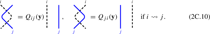
The following is our formulation of [43, Definition 2.4], [42, Definition 4.2]. Recall that we write $i\rightsquigarrow j$ if $\Gamma$ has an edge from i to j, of any multiplicity.

Definition 2C.7

The weighted KLRW algebra ${{\mathscr {W}_{{\beta }}^{{\varvec{\rho }}}}(X)}$ is the unital associative R-algebra generated (as an algebra) by the diagrams in with multiplication given by

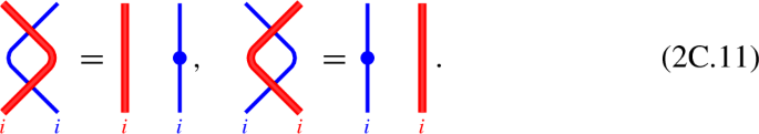
and subject to the following multilocal relations.

• (a) The dot sliding relations hold, that is, solid and ghost dots can pass through any crossing except:

  

• (b) The Reidemeister II relations hold except in the following cases:

  

  

  

• (c) The Reidemeister III relations hold except in the following cases:

  

  

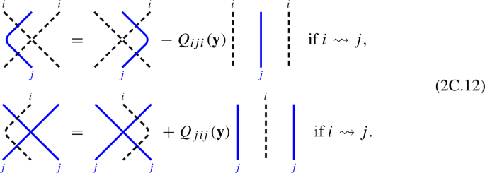
The honest Reidemeister relations are those relations in (b) and (c) where the strings satisfy the Reidemeister relations, without error terms or dots.

There is an asymmetry in (2C.11) and (2C.12) that plays an important role in Sect. 3F.

Example 2C.14

Multilocal relations can be tricky to apply. For example, it looks as if we can apply (2C.8) to the left-hand side of the following diagram:

Relation (2C.8) changes both the solid strings and their ghost strings, since the ghost strings are implicitly part of this relation. This relation cannot be applied here because every local neighborhood that contains the two ghost i-strings also contains the solid j-string.

Remark 2C.15

Note that we fixed $\beta \in Q^{+}_{n}$ of height $\textrm{ht}(\beta )=n$, which amounts to fixing the labels of the solid strings. We sometimes write

$$\begin{aligned} {\mathscr {W}_{{n}}^{{\varvec{\rho }}}}(X)= \bigoplus _{\beta \in Q^{+}_{n}}{\mathscr {W}_{{\beta }}^{{\varvec{\rho }}}}(X), \end{aligned}$$

which is a decomposition of ${{\mathscr {W}_{{\beta }}^{{\varvec{\rho }}}}(X)}$ into a direct sum of two-sided ideals. Of course, anything we say about ${{\mathscr {W}_{{\beta }}^{{\varvec{\rho }}}}(X)}$ has a corresponding statement for ${\mathscr {W}_{{n}}^{{\varvec{\rho }}}}(X)$, which we will not usually state explicitly.

2.4 The grading on ${{\mathscr {W}_{{\beta }}^{\rho }(X)}}$

Notation 2D. 1

In this paper a graded algebra or module will always mean a $\mathbb {Z}$-graded algebra or module.

Definition 2D. 2

We endow the algebra ${{\mathscr {W}_{{\beta }}^{{\varvec{\rho }}}}(X)}$ with a grading as follows. The grading is defined on the diagrams by summing over the contributions from each dot and crossing in the diagram according to the following local (not multilocal) rules:

Lemma 2D. 3

Definition 2D. 2 endows ${{\mathscr {W}_{{\beta }}^{{\varvec{\rho }}}}(X)}$ with the structure of a graded algebra.

Proof

The algebra ${{\mathscr {W}_{{\beta }}^{{\varvec{\rho }}}}(X)}$ is graded using these degrees because all of the relations in Definition 2C.7 are homogeneous with respect to the degree function from Definition 2D. 2. $\square$

From now on, we consider ${{\mathscr {W}_{{\beta }}^{{\varvec{\rho }}}}(X)}$ as a graded algebra using Definition 2D. 2.

Notation 2D. 4

Let ${{\mathscr {W}_{{\beta }}^{{\varvec{\rho }}}}(X)\text {-}\textbf{Mod}_{\mathbb {Z}}}$ be the category of graded ${{\mathscr {W}_{{\beta }}^{{\varvec{\rho }}}}(X)}$-modules, where a graded category means a category with hom-spaces enriched in the category of graded R-modules. The corresponding categories of right ${{\mathscr {W}_{{\beta }}^{{\varvec{\rho }}}}(X)}$-modules is $\textbf{Mod}_{\mathbb {Z}}\text {-}{\mathscr {W}_{{\beta }}^{{\varvec{\rho }}}}(X)$.

3 Some properties of weighted KLRW algebras

As in Notation 2C.6, we fix all of the data $\Gamma ,{\varvec{\sigma }},\beta ,X$ etc. needed to define the weighted KLRW algebra ${\mathscr {W}_{{\beta }}^{{\varvec{\rho }}}}(X)$.

3.1 First properties

Proposition 3A.1

Consider pairs $(\Gamma ,{\varvec{\sigma }})$ and $(\Gamma ^{\prime },{\varvec{\sigma }}^{\prime })$ where the quivers $\Gamma$ and $\Gamma ^{\prime }$ differ by precisely one edge $\epsilon$, which is oriented $\epsilon :i\rightsquigarrow j$ in $\Gamma$ and $\epsilon ^{\prime }:j\rightsquigarrow i$ in $\Gamma ^{\prime }$, such that $Q_{ij}(u,v)=-Q_{ji}^{\prime }(v,u)$. Let ${\mathscr {W}_{{\beta }}^{{\varvec{\rho }}}}(X)$ and ${{\mathscr {W}_{{\beta }}^{{\varvec{\rho }}}}(X)^{\prime }}$, respectively, be the corresponding weighted KLRW algebras. If $\sigma _{\epsilon }=-\sigma _{\epsilon ^{\prime }}$, then there is an isomorphism of graded algebras ${{\mathscr {W}_{{\beta }}^{{\varvec{\rho }}}}(X)\cong {\mathscr {W}_{{\beta }}^{{\varvec{\rho }}}}(X)^{\prime }}$.

Proof

The identity map on diagrams gives the required isomorphism. $\square$

Define an R-linear map ${({}_{-}){}^{\star }\,{:}\,{\mathscr {W}_{{\beta }}^{{\varvec{\rho }}}}(X)\!\longrightarrow \!{\mathscr {W}_{{\beta }}^{{\varvec{\rho }}}}(X)}$ by reflecting diagrams in the line $y=\frac{1}{2}$:

The next two easy, but important, properties are straightforward.

Lemma 3A.3

• (a) The map ${({}_{-}){}^{\star }\,{:}\,{\mathscr {W}_{{\beta }}^{{\varvec{\rho }}}}(X)\!\longrightarrow \!{\mathscr {W}_{{\beta }}^{{\varvec{\rho }}}}(X)}$ is a homogeneous algebra antiinvolution.

• (b) The map ${({}_{-}){}^{\star }\,{:}\,{\mathscr {W}_{{\beta }}^{{\varvec{\rho }}}}(X)\!\longrightarrow \!{\mathscr {W}_{{\beta }}^{{\varvec{\rho }}}}(X)}$ gives rise to equivalences of graded R-linear abelian categories

  $$\begin{aligned}&({}_{-}){}^{\star }\,{:}\,{\mathscr {W}_{{\beta }}^{{\varvec{\rho }}}}(X)\text {-}\textbf{Mod}_{\mathbb {Z}}\!\longrightarrow \!\textbf{Mod}_{\mathbb {Z}}\text {-}{\mathscr {W}_{{\beta }}^{{\varvec{\rho }}}}(X),\\&\quad ({}_{-}){}^{\star }\,{:}\,\textbf{Mod}_{\mathbb {Z}}\text {-}{\mathscr {W}_{{\beta }}^{{\varvec{\rho }}}}(X)\!\longrightarrow \!{\mathscr {W}_{{\beta }}^{{\varvec{\rho }}}}(X)\text {-}\textbf{Mod}_{\mathbb {Z}}, \end{aligned}$$

  both of which we denote by the same symbol.

Lemma 3A.4

Let be a straight line diagram. Then D is invertible in ${{\mathscr {W}_{{\beta }}^{{\varvec{\rho }}}}(X)}$, for appropriately chosen X, with inverse $D^{\star }$.

The set of positions X is a set of loadings $({\varvec{\kappa }},\varvec{x})$, where ${\varvec{\kappa }}$ is a charge and $\varvec{x}$ is a solid positioning. In particular, the loadings in X do not necessarily have the same charge, which means that the endpoints of the red strings can vary.

A set of positions Y has constant charge ${\varvec{\kappa }}$ if every loading in Y has charge ${\varvec{\kappa }}$. The next result says that we can assume that the set of positions has constant charge.

Proposition 3A.5

Suppose that X is a set of positions. Then there exists a set of positions Y of constant charge such that ${{\mathscr {W}_{{\beta }}^{{\varvec{\rho }}}}(X)\cong {\mathscr {W}_{{\beta }}^{{\varvec{\rho }}}}(Y)}$ as graded algebras.

Proof

Conjugation by straight line diagrams defines the required isomorphism by Lemma 3A.4:

Here D is a diagram in ${\mathscr {W}_{{\beta }}^{{\varvec{\rho }}}}(X)$. $\square$

Notation 3A.6

Without loss of generality, by Proposition 3A.5, we can, and will, assume that X has constant charge ${\varvec{\kappa }}$.

Let us further explain how one can vary the size of X.

Definition 3A.7

Let $\simeq$ be the equivalence relation on the set of loadings where $\varvec{x}\simeq \varvec{y}$, if for each $\textbf{i}\in I^{n}$ there exists a straight line diagram $D\in \mathbb {W}_{\varvec{x},\textbf{i}}^{\varvec{y},\textbf{i}}$. Extend $\simeq$ to the set of positionings by defining $X\simeq Y$, if for any $\varvec{x}\in X$ there exists $\varvec{y}\in Y$ such that $\varvec{x}\simeq \varvec{y}$.

Example 3A.8

Let $\varvec{x}$ and $\varvec{y}$ be the bottom and top positionings of a straight line diagram, as in (2B.14). Then $\{\varvec{x}\}\simeq \{\varvec{x},\varvec{y}\}\simeq \{\varvec{y}\}$, since $\varvec{x}\simeq \varvec{y}$. Then Proposition 3A.9 below shows that from the perspective of weighted KLRW algebras one of these loadings is redundant.

Proposition 3A.9

Suppose that $X\simeq Y$.

• (a) If $\#X=\#Y$, then ${{\mathscr {W}_{{\beta }}^{{\varvec{\rho }}}}(X)\cong {\mathscr {W}_{{\beta }}^{{\varvec{\rho }}}}(Y)}$ as graded algebras.

• (b) The algebras ${{\mathscr {W}_{{\beta }}^{{\varvec{\rho }}}}(X)}$ and ${{\mathscr {W}_{{\beta }}^{{\varvec{\rho }}}}(Y)}$ are graded Morita equivalent.

Proof

(a) Note that we can restrict to the case where X and Y differ by only one element. Then the straight line diagrams provide the corresponding isomorphism.

(b) We can restrict to the case where $\#X+1=\#Y$ and, by (a), that $X\subset Y$. Note that, by assumption, the additional element in Y is related to another element in X by a straight line diagram, which corresponds to a bimodule, showing that the corresponding graded projective ${{\mathscr {W}_{{\beta }}^{{\varvec{\rho }}}}(Y)}$-modules are graded equivalent. This together with (a) proves the claim. $\square$

Observe that the identity element of ${{\mathscr {W}_{{\beta }}^{{\varvec{\rho }}}}(X)}$ is

$$\begin{aligned} {\textbf {1}} _{\mathscr {W}}=\sum _{\varvec{x}\in X,\textbf{i}\in I^{\beta }}{\textbf {1}} _{\varvec{x},\textbf{i}}, \end{aligned}$$

and that ${{\mathscr {W}_{{\beta }}^{{\varvec{\rho }}}}(X){\textbf {1}} _{\varvec{x},\textbf{i}}}$ is a projective ${{\mathscr {W}_{{\beta }}^{{\varvec{\rho }}}}(X)}$-module, for $\varvec{x}\in X$ and $\textbf{i}\in I^{\beta }$. Note that every projective ${{\mathscr {W}_{{\beta }}^{{\varvec{\rho }}}}(X)}$-module appears as a direct summand of some projective ${{\mathscr {W}_{{\beta }}^{{\varvec{\rho }}}}(X)}$-module of the form ${{\mathscr {W}_{{\beta }}^{{\varvec{\rho }}}}(X){\textbf {1}} _{\varvec{x},\textbf{i}}}$. Moreover, for any $\varvec{x}\in X$ let ${\textbf {1}} _{\varvec{x}}=\sum _{\textbf{i}\in I^{\beta }}{\textbf {1}} _{\varvec{x},\textbf{i}}$. Then ${\textbf {1}} _{\varvec{x}}$ is an idempotent in ${{\mathscr {W}_{{\beta }}^{{\varvec{\rho }}}}(X)}$ and ${{\textbf {1}} _{\varvec{x}}{\mathscr {W}_{{\beta }}^{{\varvec{\rho }}}}(X){\textbf {1}} _{\varvec{x}}}$ and ${{\textbf {1}} _{\varvec{x},\textbf{i}}{\mathscr {W}_{{\beta }}^{{\varvec{\rho }}}}(X){\textbf {1}} _{\varvec{x},\textbf{i}}}$ are idempotent subalgebras, see Sect. 3F.

3.2 A basis of ${{\mathscr {W}_{{\beta }}^{\rho }(X)}}$

If $w\in {\mathfrak {S}_{n}}$, then a reduced expression for w is any word $w=s_{i_{1}}\ldots s_{i_{k}}$ of minimal length, for $1\le i_{j}<n$. If $w=s_{i_{1}}\ldots s_{i_{k}}$ is a reduced expression for w, then w has length k. The following permutation diagrams play an important role throughout this paper.

Definition 3B. 1

Fix $\varvec{x},\varvec{y}\in X$ and $\textbf{i},\textbf{j}\in I^{\beta }$. For each $w\in {\mathfrak {S}_{n}}$ such that $\textbf{j}=w\cdot \textbf{i}$ define a diagram as follows. First, assume as an intermediate step that ${\varvec{\kappa }}=\emptyset$, so that there are no red strings. Then connect the strings in $D_{{\varvec{\alpha }},\textbf{i}}^{{\varvec{\beta }},\textbf{j}}(w)$ from bottom to top by adding solid crossings (and their ghosts) corresponding to the fixed choice of reduced expression. Now add the red strings vertically to the diagram and, if necessary, pull each red string to the right so that it is to the right of any solid-solid, ghost-ghost and solid-ghost crossings on the strings that the red string crosses.

The diagram $D_{\varvec{x},\textbf{i}}^{\varvec{y},\textbf{j}}(w)$ depends on a choice of reduced expression, and not just on w, and on ${\varvec{\kappa }}$, but we suppress this from our notation.

Example 3B. 2

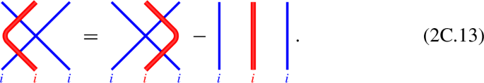
In the situation of (2C.13) we prefer the leftmost diagram, not the middle. Precisely, let $n=2$, $l=1$, ${\varvec{\kappa }}=(\tfrac{3}{2})$, ${\varvec{\kappa }}^{\prime }=(\tfrac{1}{2})$, ${\varvec{\kappa }}^{\prime \prime }=(-\tfrac{1}{2})$ and ${\varvec{\alpha }}={\varvec{\beta }}=(-1,1)$. Then, for $\textbf{i}=(i,j)$, $\textbf{j}=(j,i)$ with $i,j\in I$, and s being the unique simple reflection in ${\mathfrak {S}_{n}}$ (with s being the reduced expression) we have

By convention, all crossings on the non-red strings that cross a red string are to the left of that red string.

As in Definition 2B.15, whenever we write $D_{\varvec{x},\textbf{i}}^{\varvec{y},\textbf{j}}(w)$ we assume that $\textbf{j}=w\cdot \textbf{i}$. When $\varvec{x}$, $\varvec{y}$, $\textbf{i}$ and $\textbf{j}$ are clear from context, write $D(w)=D_{\varvec{x},\textbf{i}}^{\varvec{y},\textbf{j}}(w)$. By definition $D(w)=D(w){\textbf {1}} _{\varvec{x},\textbf{i}}={\textbf {1}} _{\varvec{y},\textbf{j}}D(w)$.

Lemma 3B. 3

The algebra ${\mathscr {W}_{{\beta }}^{{\varvec{\rho }}}}(X)$ is a finitely generated R-module and spanned by

Proposition 3B.12 below shows that (3B.4) is a basis of ${\mathscr {W}_{{\beta }}^{{\varvec{\rho }}}}(X)$.

Proof

The relations imply that the algebra ${\mathscr {W}_{{\beta }}^{{\varvec{\rho }}}}(X)$ is filtered with ${\mathscr {W}_{{\beta }}^{{\varvec{\rho }}}}(X)=\bigcup _{k\in \mathbb {Z}_{\ge 0}}{\mathscr {W}_{{\beta }}^{{\varvec{\rho }}}}(X)_{k}$, where ${\mathscr {W}_{{\beta }}^{{\varvec{\rho }}}}(X)_{k}$ is spanned by the diagrams with at most k crossings, for $k\in \mathbb {Z}_{\ge 0}$. In the associated graded algebra,

$$\begin{aligned} \hbox {gr}{\mathscr {W}_{{\beta }}^{{\varvec{\rho }}}}(X) =\bigoplus _{k>0}{\mathscr {W}_{{\beta }}^{{\varvec{\rho }}}}(X)_{k}/{\mathscr {W}_{{\beta }}^{{\varvec{\rho }}}}(X)_{k-1}, \end{aligned}$$

dots and crossing commute, double crossings satisfy the Reidemeister II relations or are zero, and the crossings satisfy the Reidemeister III relations. Therefore, the image of D(w) in $\hbox {gr}{\mathscr {W}_{{\beta }}^{{\varvec{\rho }}}}(X)$ is nonzero and depends only on w. Moreover, if D(w) and $D(w)^{\prime }$ are two such diagrams for $w\in {\mathfrak {S}_{n}}$ that are defined using different reduced expressions, then $D(w)\equiv D(w)^{\prime }\pmod {{\mathscr {W}_{{\beta }}^{{\varvec{\rho }}}}(X)_{k-1}}$, where w has length k, which is defined the be the minimal number of crossings in a permutation diagram for w. Thus, $\hbox {gr}{\mathscr {W}_{{\beta }}^{{\varvec{\rho }}}}(X)$ is spanned by the image of the set $\mathcal {B}_{\beta }$ in $\hbox {gr}{\mathscr {W}_{{\beta }}^{{\varvec{\rho }}}}(X)$, implying the result. $\square$

Remark 3B.5

Let $w\in {\mathfrak {S}_{n}}$. The proof of Lemma 3B. 3 shows that, if D(w) and $D(w)^{\prime }$ are diagrams defined using different reduced expressions for w, then $D(w)\equiv D(w)^{\prime }\pmod {{\mathscr {W}_{{\beta }}^{{\varvec{\rho }}}}(X)_{k-1}}$, where $k=\ell (w)$. By the same argument, if $D(w)^{\prime }$ is a diagram defined in the same way as D(w) except that the red strings are pulled to the left in Definition 3B. 1, then D(w) and $D(w)^{\prime }$ agree modulo ${\mathscr {W}_{{\beta }}^{{\varvec{\rho }}}}(X)_{k-1}$.

Example 3B.6

Consider the quiver $\Gamma$ as in (2A.6), and let $n=2$ and $\ell =1$. Let the solid strings have positions $\varvec{x}=(0,0.75)$ and place the red string at 1.5. Recall from Example 2A.9 that there are six choices of $\beta$. Let $\beta =\alpha _{0}+\alpha _{1}$. Then

where a and b specify the number of dots. (The ghost strings have the same number of dots.)

To show that $\mathcal {B}_{\beta }$ is a basis of ${\mathscr {W}_{{\beta }}^{{\varvec{\rho }}}}(X)$ we introduce a faithful polynomial module of ${\mathscr {W}_{{\beta }}^{{\varvec{\rho }}}}(X)$, following the standard approach in this setting, for example see [35, §3.2.2], [21, §2.3] or [43, §2.2]. Fix indeterminates $y_{1},\ldots ,y_{n}$ over R and let

$$\begin{aligned} P_{\beta }(X)= \bigoplus _{\varvec{x}\in X,\textbf{i}\in I^{\beta }} R[y_{1},\ldots ,y_{n}]{\textbf {1}} _{\varvec{x},\textbf{i}} \end{aligned}$$

be $\#(X\times I^{\beta })$ copies of the polynomial ring $R[y_{1},\ldots ,y_{n}]$, where $y_{r}{\textbf {1}} _{\varvec{x},\textbf{i}}$ has degree $2d_{i_{r}}$, for $1\le r\le n$; cf. Definition 2D. 2. The symmetric group ${\mathfrak {S}_{n}}$ acts on $P_{\beta }(X)$ by place permutations. In particular, if $1\le r<s<n$ let (r, s) be the operator that interchanges $y_{r}{\textbf {1}} _{\varvec{x},\textbf{i}}$ and $y_{s}{\textbf {1}} _{\varvec{y},\textbf{i}}$ and fixes $y_{t}{\textbf {1}} _{\varvec{x},\textbf{i}}$ for $t\ne r,s$.

Definition 3B.7

Define an assignment, using local (not multilocal) rules, from ${\mathscr {W}_{{\beta }}^{{\varvec{\rho }}}}(X)$ to $P_{\beta }(X)$ by specifying that

and all crossings act as the identity except that

where $\partial _{r,s}=\frac{(r,s)-1}{y_{s}-y_{r}}$ is the Demazure operator.

We call $P_{\beta }(X)$ the polynomial module of ${\mathscr {W}_{{\beta }}^{{\varvec{\rho }}}}(X)$. Note that the action of the crossings maps $R[y_{1},\ldots ,y_{n}]{\textbf {1}} _{\varvec{x},\textbf{i}}$ to $R[y_{1},\ldots ,y_{n}]{\textbf {1}} _{\varvec{y},\textbf{j}}$ for related $\textbf{i}$ and $\textbf{j}$. Similarly we define:

Definition 3B.10

Define an assignment, using local rules, from $\hbox {gr}{\mathscr {W}_{{\beta }}^{{\varvec{\rho }}}}(X)$ to $P_{\beta }(X)$ by using the assignment in (3B.8), but instead of (3B.9) we let

and all other crossings act as the identity.

Lemma 3B.11

There is an action of ${\mathscr {W}_{{\beta }}^{{\varvec{\rho }}}}(X)$ on $P_{\beta }(X)$ given by

where we apply the local rules from Definition 3B.7 to $P_{\beta }(X)$ by reading the crossings in D in order from bottom to top. Similarly, $\hbox {gr}{\mathscr {W}_{{\beta }}^{{\varvec{\rho }}}}(X)$ acts on $P_{\beta }(X)$ via Definition 3B.10.

Proof

Both claims follow by what is now a standard check of the relations, such as in [21, §2.3], with the slight caveat that solid strings might have associated ghost strings. For example, whenever a ghost crossing appears in one of the relations then so does its solid crossing. Explicitly, for an appropriate choice of ghost shifts and $i,j\in I^{\beta }$, (2C.12) becomes

Hence, the action of the two sides of this relation coincide because

$$\begin{aligned} \partial _{r,s}\big (Q_{ij}(r,t)f\big ) = Q_{ij}(s,t)\partial _{r,s}(f) -Q_{iji}(r,t,s), \end{aligned}$$

where we have named the solid strings r, s, and t in order. Note that this requires the Leibniz rule for $\partial _{r,s}$. That is, $\partial _{r,s}\big (Q_{ij}(r,t)f\big )= Q_{ij}(r,t)\partial _{r,s}(f)+\big ((r,s)\centerdot f\big )\partial _{r,s}\big (Q_{ij}(r,t)\big )$. $\square$

Recall the set $\mathcal {B}_{\beta }$ from (3B.4).

Proposition 3B.12

The algebra ${\mathscr {W}_{{\beta }}^{{\varvec{\rho }}}}(X)$ is free as an R-module with homogeneous basis $\mathcal {B}_{\beta }$.

Proof

By Lemma 3B. 3 the elements in $\mathcal {B}_{\beta }(X)$ span ${\mathscr {W}_{{\beta }}^{{\varvec{\rho }}}}(X)$. Hence, it remains to show that $\mathcal {B}_{\beta }(X)$ is linearly independent and for this it is sufficient to show that the images of $\mathcal {B}_{\beta }(X)$ in $\hbox {gr}{\mathscr {W}_{{\beta }}^{{\varvec{\rho }}}}(X)$ are linearly independent. Using the action of $\hbox {gr}{\mathscr {W}_{{\beta }}^{{\varvec{\rho }}}}(X)$ on $P_{\beta }(X)$, cf. Definition 3B.10, we see that D(w) acts by sending $f(y_{1},\ldots ,y_{n})$ to $f(y_{w(1)},\ldots ,y_{w(n)})$. Hence, the elements of $\mathcal {B}_{\beta }(X)$ map to linearly independent automorphisms of $R[y_{1},\ldots ,y_{n}]$ because $R[y_{1},\ldots ,y_{n}]$ is free as a module over itself. $\square$

As an immediate corollary of Proposition 3B.12 we obtain:

Corollary 3B.13

The polynomial module $P_{\beta }(X)$ is a faithful ${\mathscr {W}_{{\beta }}^{{\varvec{\rho }}}}(X)$-module.

Remark 3B.14

Note that the basis of Proposition 3B.12 is a homogeneous basis. On the other hand, $P_{\beta }(X)$ is not a graded ${\mathscr {W}_{{\beta }}^{{\varvec{\rho }}}}(X)$-module. However, $P_{\beta }(X)$ is a graded $\hbox {gr}{\mathscr {W}_{{\beta }}^{{\varvec{\rho }}}}(X)$-module.

3.3 The center of ${{\mathscr {W}_{{\beta }}^{\rho }(X)}}$

Let $R[y_{1},\ldots ,y_{a}]^{{\mathfrak {S}_{a}}}$ be the ring of symmetric polynomials in $y_{1},\ldots ,y_{a}$, where $a\in \mathbb {Z}_{\ge 1}$. For $\beta =\sum _{i\in I}a_{i}\alpha _{i}$, let $R[\beta ]^{{\mathfrak {S}_{\beta }}}=\bigotimes _{i\in I}R[y_{1},\ldots ,y_{a_{i}}]^{{\mathfrak {S}_{a_{i}}}}$. By Proposition 3B.12, we can view $R[\beta ]^{{\mathfrak {S}_{\beta }}}$ as a graded subalgebra of ${\mathscr {W}_{{\beta }}^{{\varvec{\rho }}}}(X)$ via the map $f\mapsto f{\textbf {1}} _{\mathscr {W}}$.

Example 3C.1

Recall from Example 2A.9 that $\beta _{ij}=\alpha _{i}+\alpha _{j}$ and $\beta _{i}=2\alpha _{i}$, for $i,j\in I$. Then the generators for $R[\beta _{ij}]^{{\mathfrak {S}_{\beta _{ij}}}}$ are

and the generators for $R[\beta _{i}]^{{\mathfrak {S}_{\beta _{i}}}}$ are

for suitable choices of ghost shifts etc.

Let $Z({}_{-})$ be the center.

Lemma 3C.2

Let $\Gamma$ be of type $A^{(1)}_{1}$ and ${\varvec{\kappa }}=\emptyset$. Then there is an isomorphism of graded algebras

$$\begin{aligned} Z\bigl ({\mathscr {W}_{{\beta }}^{{\varvec{\rho }}}}(X)\bigr ) \cong R[y_{1},\ldots ,y_{n}]^{{\mathfrak {S}_{n}}}. \end{aligned}$$

Proof

By Proposition 3A.9, if ${\varvec{\kappa }}=\emptyset$, then ${\mathscr {W}_{{\beta }}^{{\varvec{\rho }}}}(X)$ is Morita equivalent to the nil Hecke algebra for any choice of positions for X. Hence, we can prove this statement mutatis mutandis as for the nil Hecke algebra, see [30, Section 2] and [28, Proposition 3.5]. $\square$

Almost exactly as in [21, Theorem 2.9] we have the following.

Proposition 3C.3

There is an isomorphism $Z\bigl ({\mathscr {W}_{{\beta }}^{{\varvec{\rho }}}}(X)\bigr )\cong R[\beta ]^{{\mathfrak {S}_{\beta }}}$ of graded algebras given by

$$\begin{aligned} \nu :R[\beta ]^{{\mathfrak {S}_{\beta }}}\rightarrow Z\bigl ({\mathscr {W}_{{\beta }}^{{\varvec{\rho }}}}(X)\bigr ), f\mapsto f{\textbf {1}} _{\mathscr {W}}. \end{aligned}$$

Moreover, ${\mathscr {W}_{{\beta }}^{{\varvec{\rho }}}}(X)$ is free and of finite rank over its center.

Proof

Using the relations in Definition 2C.7 it is easy to see that for any symmetric polynomial $f\in R[\beta ]^{{\mathfrak {S}_{\beta }}}$ the element $f{\textbf {1}} _{\mathscr {W}}$ is central. The only relation for which commutativity is not immediate is (2C.8) and, in this situation, symmetrically placed dots slide freely. Hence, $\nu$ is a well-defined algebra homomorphism and it is injective by Proposition 3B.12.

Let ${\textbf {1}} _{X,\textbf{i}}=\sum _{\varvec{x}\in X}{\textbf {1}} _{\varvec{x},\textbf{i}}$. Using the same arguments as in [21, Theorem 2.9] to prove that $\nu$ is surjective it suffices to show that the composition

$$\begin{aligned} R[\beta ]^{{\mathfrak {S}_{\beta }}} \xrightarrow {\nu } Z\bigl ({\mathscr {W}_{{\beta }}^{{\varvec{\rho }}}}(X)\bigr ) \xrightarrow {{\textbf {1}} _{X,\textbf{i}}({}_{-}){\textbf {1}} _{X,\textbf{i}}} Z\bigl ({\textbf {1}} _{X,\textbf{i}}{\mathscr {W}_{{\beta }}^{{\varvec{\rho }}}}(X){\textbf {1}} _{X,\textbf{i}}\bigr ) \end{aligned}$$

is an isomorphism for all $\textbf{i}\in I^{\beta }$, where $\textbf{i}=(\underbrace{i_{1},\ldots ,i_{1}}_{a_{1}},\ldots ,\underbrace{i_{r},\ldots ,i_{r}}_{a_{r}})$. For such $\textbf{i}$ we have

$$\begin{aligned} {\textbf {1}} _{X,\textbf{i}}{\mathscr {W}_{{\beta }}^{{\varvec{\rho }}}}(X){\textbf {1}} _{X,\textbf{i}} \cong \bigotimes _{k=1}^{r} {\mathscr {W}_{{a_{k}}}^{{\varvec{\rho }}}}(X), \end{aligned}$$

where each algebra appearing on the right-hand side is the subalgebra of ${\textbf {1}} _{X,\textbf{i}}{\mathscr {W}_{{\beta }}^{{\varvec{\rho }}}}(X){\textbf {1}} _{X,\textbf{i}}$ having only identities outside of the indicated region. Hence, we have identified the center since, by Lemma 3C.2, the center of ${\mathscr {W}_{{a_{k}}}^{{\varvec{\rho }}}}(X)$ is $R[y_{1},\ldots ,y_{a_{k}}]^{{\mathfrak {S}_{a_{k}}}}$.

The final claim now follows from Proposition 3B.12. $\square$

Standard arguments now yield:

Proposition 3C.4

• (a) The algebra ${\mathscr {W}_{{\beta }}^{{\varvec{\rho }}}}(X)$ is left and right Noetherian.

• (b) The algebra ${\mathscr {W}_{{\beta }}^{{\varvec{\rho }}}}(X)$ is indecomposable.

• (c) Suppose that R is a field. Then every simple ${\mathscr {W}_{{\beta }}^{{\varvec{\rho }}}}(X)$-module is finite dimensional.

3.4 Cyclotomic quotients

We now define cyclotomic or steadied quotients of ${\mathscr {W}_{{\beta }}^{{\varvec{\rho }}}}(X)$. As we will see in Proposition 3F.1, these quotients generalize cyclotomic KLR(W) algebras.

Recall that X is the set of allowable endpoints of the solid and red strings. A string is bounded by X if the x-coordinates of its points are bounded, on the left and right, by the x-coordinates of the points in X.

Definition 3D.1

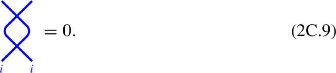
A diagram ${\textbf {1}} _{\varvec{x},\textbf{i}}$ is (right) unsteady if it contains a solid string that can be pulled arbitrarily far to the right when the red strings are bounded by X. A diagram is unsteady if it contains an unsteady string and otherwise it is steady.

Definition 3D.2

The cyclotomic weighted KLRW algebra ${\mathscr {R}_{{\beta }}^{{\varvec{\rho }}}}(X)$ is the quotient of ${\mathscr {W}_{{\beta }}^{{\varvec{\rho }}}}(X)$ by the two-sided ideal generated by all diagrams that factor through an unsteady idempotent diagram.

Similarly, we define left unsteady diagrams. Reflecting diagrams shows that a quotient algebra that is defined by factoring out by the two-sided ideal of diagrams that factor through some left unsteady idempotent diagram is isomorphic to a cyclotomic weighted KLRW algebra and vice versa. We work with right unsteady diagrams because we already have a left-right bias for the ghosts strings in Definition 2B.6.

Example 3D.3

If $\rho =i$, then following diagrams are unsteady and steady, respectively.

In the right-hand diagram the solid string cannot be pulled further to the right because it cannot be pulled past the red string, so the diagram is steady. However, if $\rho \ne i$ we can use (2C.11):

Hence, if $\rho \ne i$, then both of the diagrams above are unsteady, and so zero in ${\mathscr {R}_{{\beta }}^{{\varvec{\rho }}}}(X)$.

We abuse notation and identify the elements of ${\mathscr {W}_{{\beta }}^{{\varvec{\rho }}}}(X)$ with their images in ${\mathscr {R}_{{\beta }}^{{\varvec{\rho }}}}(X)$.

Proposition 3D.4

The algebra ${\mathscr {R}_{{\beta }}^{{\varvec{\rho }}}}(X)$ is finite dimensional.

Proof

By Proposition 3B.12, the algebra ${\mathscr {R}_{{\beta }}^{{\varvec{\rho }}}}(X)$ is spanned by the image of $\mathcal {B}_{\beta }$ in ${\mathscr {R}_{{\beta }}^{{\varvec{\rho }}}}(X)$. Hence, it is enough to show that the dotted idempotent $y_{1}^{a_{1}}\ldots y_{n}^{a_{n}}{\textbf {1}} _{\varvec{x},\textbf{i}}$ is zero when $a_{1},\ldots ,a_{n}\in \mathbb {Z}_{\ge 0}$ are big enough. We prove this by induction on the number $\ell$ of red strings. If $\ell =0$, then any diagram is unsteady and the claim follows. If $\ell >0$, then take the leftmost red string and record the minimal number m of dots that we need to add to the solid strings so that (2C.11) can be applied to pull the red string to the left of all of the solid strings. Now remove this red string from the diagram. By induction there exist $a_{1}^{\prime },\ldots ,a_{n}^{\prime }$ annihilating the dotted idempotent. Setting $a_{r}=a_{r}^{\prime }+m$ now implies that $y_{1}^{a_{1}}\ldots y_{n}^{a_{n}}{\textbf {1}} _{\varvec{x},\textbf{i}}=0$, completing the proof. $\square$

As we will see below, the unsteady condition, which crucially depends on the choice of red strings, corresponds to the cyclotomic ideal in the KLR world. It is difficult to tell what elements belong to the cyclotomic ideal. In contrast, as we will see it is very easy to tell when a diagram is unsteady, which is one of the main advantages of the weighted KLRW framework.

3.5 Induction and restriction

We now discuss the analog of [21, Section 2.6] and [43, Section 2.4] for weighted KLRW algebras, which apply almost without change. To this end, recall that X is a set of positionings. For each such set and each $z\in \mathbb {R}$ we let $X\{ z\}=\{ \varvec{x}+z|\varvec{x}\in X\}$ be the set of shifted positionings. More generally, set $XY\{z\}=X\cup (Y\{z\})$ (we use similar notations below) and let $\textrm{d}(X,Y)=\max (X)-\min (Y)$, where $\min$ and $\max$ have the obvious meanings.

The following is clear from Proposition 3B.12.

Proposition 3E.1

For $\beta ,\beta ^{\prime }\in Q^{+}$ and $z>\textrm{d}(X,X^{\prime })\in \mathbb {R}$, we have an embedding of graded algebras

Moreover, $\iota _{\beta ,\beta ^{\prime }}=\iota _{\beta ,\beta ^{\prime }}({\textbf {1}} _{\mathscr {W}}\otimes {\textbf {1}} _{{\mathscr {W}_{\beta ^{\prime }}^{{\varvec{\rho }}^{\prime }}}(X^{\prime })})$ is an idempotent.$\square$

For any $z>\textrm{d}(X,X^{\prime })\in \mathbb {R}$ we have a restriction functor

$$\begin{aligned} \mathcal {F}_{*}^{\beta ,\beta ^{\prime }}\,{:}\,{\mathscr {W}_{\beta +\beta ^{\prime }}^{{\varvec{\rho }}}}(XX^{\prime }\{z\})\text {-} \textbf{Mod}_{\mathbb {Z}}\!\longrightarrow \!\bigl ({\mathscr {W}_{{\beta }}^{{\varvec{\rho }}}}(X)\otimes {\mathscr {W}_{\beta ^{\prime }}^{{\varvec{\rho }}^{\prime }}}(X^{\prime })\bigr )\text {-}\textbf{Mod}_{\mathbb {Z}}, \end{aligned}$$

that sends M to $\iota _{\beta ,\beta ^{\prime }}M$. There are also induction and coinduction functors

$$\begin{aligned}&\mathcal {F}^{!}_{\beta ,\beta ^{\prime }}\,{:}\,\bigl ({\mathscr {W}_{{\beta }}^{{\varvec{\rho }}}}(X)\otimes {\mathscr {W}_{\beta ^{\prime }}^{{\varvec{\rho }}^{\prime }}}(X^{\prime })\bigr )\text {-}\textbf{Mod}_{\mathbb {Z}}\!\longrightarrow \!{\mathscr {W}_{\beta +\beta ^{\prime }}^{{\varvec{\rho }}}}(XX^{\prime }\{z\})\text {-}\textbf{Mod}_{\mathbb {Z}}, \\&\mathcal {F}^{!}_{\beta ,\beta ^{\prime }}={\mathscr {W}_{{\beta }}^{{\varvec{\rho }}}}(XX^{\prime }\{z\})\iota _{\beta ,\beta ^{\prime }} \otimes _{{\mathscr {W}_{{\beta }}^{{\varvec{\rho }}}}(X)\otimes {\mathscr {W}_{{\beta }}^{{\varvec{\rho }}}}(X^{\prime })}{}_{-}, \\&\mathcal {F}^{*}_{\beta ,\beta ^{\prime }}\,{:}\,\bigl ({\mathscr {W}_{{\beta }}^{{\varvec{\rho }}}}(X)\otimes {\mathscr {W}_{\beta ^{\prime }}^{{\varvec{\rho }}^{\prime }}}(X^{\prime })\bigr )\text {-}\textbf{Mod}_{\mathbb {Z}}\!\longrightarrow \!{\mathscr {W}_{{\beta }}^{{\varvec{\rho }}}}(XX^{\prime }\{z\})\text {-}\textbf{Mod}_{\mathbb {Z}}, \\&\mathcal {F}^{*}_{\beta ,\beta ^{\prime }}=\textrm{Hom}_{({\mathscr {W}_{{\beta }}^{{\varvec{\rho }}}}(X)\otimes {\mathscr {W}_{\beta ^{\prime }}^{{\varvec{\rho }}^{\prime }}}(X^{\prime }))\text {-}\textbf{Mod}_{\mathbb {Z}}}\big ({\mathscr {W}_{\beta +\beta ^{\prime }}^{{\varvec{\rho }}}}(XX^{\prime }\{z\}),{}_{-}\big ) . \end{aligned}$$

Remark 3E.2

A straight line diagram argument implies that the functors $\mathcal {F}_{*}^{\beta ,\beta ^{\prime }}$, $\mathcal {F}^{!}_{\beta ,\beta ^{\prime }}$ and $\mathcal {F}^{*}_{\beta ,\beta ^{\prime }}$ do not depend on z, which is why we do not include z in the notation.

Let $P_{\varvec{x},\textbf{i}}={\mathscr {W}_{{\beta }}^{{\varvec{\rho }}}}(X){\textbf {1}} _{\varvec{x},\textbf{i}}$ be the projective ${\mathscr {W}_{{\beta }}^{{\varvec{\rho }}}}(X)$-module generated by the idempotent ${\textbf {1}} _{\varvec{x},\textbf{i}}$.

Proposition 3E.3

• (a) The functor $\mathcal {F}^{!}_{\beta ,\beta ^{\prime }}$ is the left adjoint of $\mathcal {F}_{*}^{\beta ,\beta ^{\prime }}$.

• (b) The functor $\mathcal {F}^{*}_{\beta ,\beta ^{\prime }}$ is the right adjoint of $\mathcal {F}_{*}^{\beta ,\beta ^{\prime }}$.

• (c) The functors $\mathcal {F}_{*}^{\beta ,\beta ^{\prime }}$, $\mathcal {F}^{!}_{\beta ,\beta ^{\prime }}$ and $\mathcal {F}^{*}_{\beta ,\beta ^{\prime }}$ are R-linear additive and homogeneous.

• (d) The functor $\mathcal {F}_{*}^{\beta ,\beta ^{\prime }}$ is exact, $\mathcal {F}^{!}_{\beta ,\beta ^{\prime }}$ is right exact and $\mathcal {F}^{*}_{\beta ,\beta ^{\prime }}$ is left exact.

• (e) We have $\mathcal {F}^{!}_{\beta ,\beta ^{\prime }}(P_{\varvec{x},\textbf{i}}\otimes P_{\varvec{y},\textbf{j}})\cong P_{\varvec{x}\varvec{y}\{z\},\textbf{i}\textbf{j}}$ as graded ${\mathscr {W}_{\beta +\beta ^{\prime }}^{{\varvec{\rho }}}}(XX^{\prime }\{z\})$-modules.

• (f) For $\varvec{z}=\varvec{x}\varvec{y}\{z\}$ we have $\mathcal {F}_{*}^{\beta ,\beta ^{\prime }}(P_{\varvec{z},\textbf{k}})\cong \bigoplus _{\textbf{i}*\textbf{j}=\textbf{k}}(P_{\varvec{x},\textbf{i}}\otimes P_{\varvec{y},\textbf{j}})$ as graded ${\mathscr {W}_{{\beta }}^{{\varvec{\rho }}}}(X)\otimes {\mathscr {W}_{\beta ^{\prime }}^{{\varvec{\rho }}}}(X^{\prime })$-modules, where the direct sum runs over all shuffles of $\textbf{k}$ (see [21, Section 2.6]).

Proof

The first four statements follow from the usual Yoga, while the final two claims can be proven mutatis mutandis as in [21, Section 2.6]. $\square$

3.6 Relationship to (non-weighted) KLRW algebras

Let $\mathcal {W}_{{\beta }}^{{{\varvec{\rho }}}}$ be Webster’s tensor product algebra attached to the datum $\beta$ for solid, and ${\varvec{\kappa }}$ and ${\varvec{\rho }}$ for red strings. We will not recall the definition of $\mathcal {W}_{{\beta }}^{{{\varvec{\rho }}}}$, which is given in [41, Chapter 4] via string diagrams. We note that ${{\mathcal {W}}_{n}^{{{\varvec{\rho }}}}}$ is the algebra $\tilde{T}_{n}^{\lambda }$ in Webster’s notation; see (2C.15). By [41, Theorem 4.18], the algebra $\mathcal {W}_{{\beta }}^{{{\varvec{\rho }}}}$ is a generalization of the KLR algebra attached to $\beta$ [21, 35], so we call $\mathcal {W}_{{\beta }}^{{{\varvec{\rho }}}}$ a KLRW algebra. Let $\mathcal {R}_{{\beta }}^{{{\varvec{\rho }}}}$ be the cyclotomic quotient of $\mathcal {W}_{{\beta }}^{{{\varvec{\rho }}}}$, as defined in [41, Chapter 4]. Finally, the algebra $\mathcal {W}_{{\beta }}^{{{\varvec{\rho }}}}$ has a relation that is a symmetric version of (2C.11), which will be crucial in the proof of Proposition 3F.1 below. Namely:

regardless of the orientation of the underlying quiver. The definition of $\mathcal {W}_{{\beta }}^{{{\varvec{\rho }}}}$ and $\mathcal {R}_{{\beta }}^{{{\varvec{\rho }}}}$ also involves a choice of positions $(\varvec{x},{\varvec{\kappa }})$ for the strands in [41, Chapter 4]. By conjugating by straight line diagrams, we can assume that $\varvec{x}=(x_{1},\ldots ,x_{n})$ are nonintegral points and that ${\varvec{\kappa }}$ consists of integral points. We call this a KLRW positioning.

The following should be compared with [43, Proposition 2.14].

Proposition 3F.1

Let $X\simeq \{ \varvec{x}\}$ where $\varvec{x}$ is a KLRW positioning. Suppose that we are in the infinitesimal-case and $\Gamma$ has no parallel edges. We also fix one choice of Q-polynomials.

• (a) The algebras $\mathcal {W}_{{\beta }}^{{{\varvec{\rho }}}}$ and ${\mathscr {W}_{{\beta }}^{{\varvec{\rho }}}}(X)$ are graded Morita equivalent.

• (b) Furthermore, for any $\varvec{y}\in X$ with $\varvec{x}\simeq \varvec{y}$, we have an isomorphism of graded algebras

  

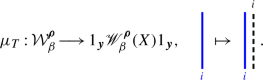
• (c) The isomorphism $\mu _{T}$ descends to an isomorphism of graded algebras $\tilde{\mu }_{T}\,{:}\,\mathcal {R}_{{\beta }}^{{{\varvec{\rho }}}}\!\longrightarrow \!1_{\varvec{y}}{\mathscr {R}_{{\beta }}^{{\varvec{\rho }}}}(X)1_{\varvec{y}}$.

Proof

(Sketch of proof.) The assignment $\mu _{T}$ is clearly homogeneous. Moreover, we can use the polynomial module to show that $\mu _{T}$ is injective, and thus bijective, by Proposition 3B.12 and [41, Proposition 4.16], which is the corresponding statement for $\mathcal {W}_{{\beta }}^{{{\varvec{\rho }}}}$. Hence, it suffices to prove that $\mu _{T}$ is well-defined. This follows from the combinatorics of how solid and ghost strings interact. For example, we have

for the two orientations given above. The left-hand side is a defining relation in $\mathcal {W}_{{\beta }}^{{{\varvec{\rho }}}}$, the right-hand side is a relation in ${\mathscr {W}_{{\beta }}^{{\varvec{\rho }}}}(X)$, which holds by (2C.11) and the fact that solid-solid and ghost-ghost strings satisfy the Reidemeister II relation. In more detail, for the two orientations considered above we have:

where we have straightened some of the i-strings to improve readability. Note that the appearance of the Q-polynomial in the ${\mathscr {W}_{{\beta }}^{{\varvec{\rho }}}}(X)$ relations depends on the orientation. Moreover, the ghost j-string and solid i-string, do not play a role in these calculations, so this argument also works when these ghost strings do not appear. Note that multiple ghosts i or j-strings do not affect the argument as the relations of ${\mathscr {W}_{{\beta }}^{{\varvec{\rho }}}}(X)$ depend on edges in the quiver and not on the vertices. (This calculation requires the assumption that $\Gamma$ does not have parallel edges.) All other relations can be checked mutatis mutandis, proving (b). The claim in (a) now follows from (b) using Proposition 3A.9. For the final claim, observe that $\mu _{T}$ gives a bijection between unsteady diagrams for the two algebras. $\square$

Example 3F.2

Let $\Gamma$ be $A_{\mathbb {Z}}$ or $A_{e}^{(1)}$ in (2A.5). Let $\ell =1$, $\varvec{x}=0.9\cdot (1,\ldots ,n)$ and $\kappa =(n)$. Let ${\varvec{\sigma }}$ be constant 0.01 and define $Q_{ij}(\textbf{y})$ as in (2C.5). Then ${\textbf {1}} _{\varvec{x}}{\mathscr {W}_{{\beta }}^{{\varvec{\rho }}}}(X){\textbf {1}} _{\varvec{x}}$ is graded isomorphic to the KLR algebra from [21] or [35] of the corresponding type.

For the rest of the paper we will identify ${\textbf {1}} _{\varvec{x}}{\mathscr {W}_{{\beta }}^{{\varvec{\rho }}}}(X){\textbf {1}} _{\varvec{x}}$ and the KLR(W) algebras of [21, 35, 41] using the choices in Proposition 3F.1. Similarly, we also identify the cyclotomic quotients of these algebras.

Remark 3F.3

For suitable choices of X, the KLR algebra is an idempotent subalgebra of ${\mathscr {W}_{{\beta }}^{{\varvec{\rho }}}}(X)$ and the cyclotomic KLR algebra is an idempotent subalgebra of ${\mathscr {R}_{{\beta }}^{{\varvec{\rho }}}}(X)$. In particular, the weighted KLRW algebras and KLR algebras usually have different numbers of simple modules.

4 Varying the quiver

The aim of this section is to define isomorphisms between weighted KLRW algebras attached to different quivers. Our main definition is Definition 4C.4 and partially inspired by [11, 29]. The isomorphism in Theorem 4D.2 makes it possible to compare the representation theories of weighted KLRW algebras for different quivers, for example for quivers of types $A^{(1)}_{e-1}$ and $A^{(1)}_{e}$. Before coming to the generalization of these results, for completeness, we briefly discuss a much easier (but less interesting), way to vary the quiver.

4.1 Another induction and restriction

We keep using the conventions in Notation 2A.2.

Definition 4A.1

Let $\Gamma =(\Gamma ,{\varvec{\sigma }})$ and ${\Gamma }^{!}=({\Gamma }^{!},{{\varvec{\sigma }}}^{!})$ be two quivers as in Sect. 2A together with a choice of ghost shifts. Then ${\Gamma }^{!}$ is an induction of $\Gamma$ and $\Gamma$ is a restriction of ${\Gamma }^{!}$ if $\Gamma$ is a weighted subgraph (cf. (2B.4)) of ${\Gamma }^{!}$.

Example 4A.2

If $d<e$, then $(A_{d},{\varvec{\sigma }})$ is a restriction of $(A^{(1)}_{e},{{\varvec{\sigma }}}^{!})$. In contrast, the quiver $A^{(1)}_{d}$ is an induction or a restriction of the quiver $A^{(1)}_{e}$ if and only if $e=d$ (and the ghost shifts match).

In the following we write ${{}_{-}}^{!}$ for everything related to ${\Gamma }^{!}$.

Proposition 4A.3

For any induction ${\Gamma }^{!}$ we have an embedding and a projection of graded algebras

$$\begin{aligned} {f}^{!}:{\mathscr {W}_{n}^{\rho }}(X)\hookrightarrow {{\mathscr {W}_{n}^{\rho }}(X)}^{!}, \quad {f}_{*}:{{\mathscr {W}_{n}^{\rho }}(X)}^{!}\twoheadrightarrow {\mathscr {W}_{n}^{\rho }}(X), \end{aligned}$$

given by sending each generator of ${\mathscr {W}_{n}^{\rho }}(X)$ to the same named element in ${{\mathscr {W}_{n}^{\rho }}(X)}^{!}$ respectively by annihilation ${\textbf {1}} _{\varvec{x},\textbf{i}}$ for $\textbf{i}$ with $i_{k}\in {I}^{!}\setminus I$ for some $k=1,\ldots ,n$. Moreover, ${f}_{*}\circ {f}^{!}=\textrm{Id}_{{\mathscr {W}_{n}^{\rho }}(X)}$.

Proof

The only claim that is not immediate by construction is that ${f}^{!}$ is an embedding. This however follows from Proposition 3B.12. $\square$

We thus get the associated restriction, induction and coinduction functors, and the analog of Proposition 3E.1, all of which we leave to the reader to spell out.

4.2 Subdividing quivers

Now we come to one of our main definitions.

Definition 4B.1

We call a subdivision of the simply laced edge .

Definition 4B.2

Let $\Gamma$ and $\bar{\Gamma }$ be two quivers as in Sect. 2A. Then $\bar{\Gamma }$ is a (simply laced) subdivision of $\Gamma$ if $\bar{\Gamma }$ is obtained from $\Gamma$ by subdividing a finite number of simply laced edges and, potentially, relabeling the vertices.

By definition, any subdivision of $\Gamma$ is obtained by successively replacing edges in a quiver with . In particular, the orientations of the subdivided edges are compatible with the original orientation of the subdivided edge.

Example 4B.3

With respect to the quivers in (2A.5) we have:

• (a) The quiver $A_{\mathbb {Z}}$ is a subdivision of itself.

• (b) If $e\ge d$, then the quiver $A^{(1)}_{e}$ is a subdivision of $A^{(1)}_{d}$. (Compare with Example 4A.2.)

• (c) The quiver $C_{\mathbb {Z}_{\ge 0}}$ is a subdivision of itself since we only subdivide simply laced edges.

• (d) If $e\ge d$, then the quiver $C^{(1)}_{e}$ is a subdivision of $C^{(1)}_{d}$.

• (e) Conversely, any subdivision of the quivers in (a)–(d) is a quiver of the same kind.

Notation 4B.4

As a general rule, we place a bar above all of the associated Cartan data for the quiver $\bar{\Gamma }$. For example, $\bar{Q}^{+}=\bigoplus _{i\in \bar{I}}\mathbb {Z}_{\ge 0}\bar{\alpha }_{i}$, and so on.

For $\Gamma$ we fix a subdivision $\bar{\Gamma }$. Subdivision determines two injective maps, denoted by the same symbol, $S\,{:}\,I\!\longrightarrow \!\bar{I}$ and $S\,{:}\,E\!\longrightarrow \!\bar{E}$, such that if $r:i\rightarrow j$ is in E, then

is the subdivided edge in $\bar{E}$. In particular, the edge $r:i\rightarrow j$ in $\Gamma$ is replaced with k edges in $\bar{\Gamma }$.

Definition 4B.5

Let $\beta =\sum _{i\in I_{\Gamma }}b_{i}\alpha _{i}\in Q^{+}_{\Gamma }$. Define

$$\begin{aligned} \bar{\beta }=\sum _{i\in I_{\Gamma }}b_{i}\bar{\alpha }_{S(i)} \in Q^{+}_{\bar{\Gamma }}. \end{aligned}$$

Example 4B.6

Consider the quiver $\Gamma$ from (2A.6), and the two subdivisions given by

The subdivision map $S$ sends i to i, so all of the original edges keep their name, and $\bar{\beta }=\beta$ using the Kac–Moody data for $\bar{\Gamma }$ rather than $\Gamma$. For $\bar{\Gamma }^{\prime }$, the map $S'$ sends $0\mapsto 0$, $1\mapsto 2$, and $2\mapsto 3$, so that the edges of $\Gamma$, and the subscripts of $\beta$, change accordingly.

To apply subdivision to weighted KLRW algebras we need to add a weighting to the subdivided quiver.

Definition 4B.7

Let $\Gamma$ be an admissible quiver and let ${\varvec{\sigma }}$ be a ghost shift for $\Gamma$. Given a weighted simply laced edge in $\Gamma$, let be weighted subdivision of this edge, where $\bar{\sigma }\in \mathbb {R}_{\ne 0}$.

We define weighted (simply laced) subdivisions of $\Gamma$ accordingly, and we use the terminology of subdivision and weighted subdivision interchangeably. We note also that we will make a choice of $\Gamma$ and a subdivision $\bar{\Gamma }$, but omit these from the notation.

4.3 Subdividing weighted KLRW diagrams

In view of the paragraph after Definition 4B.2, throughout this section we restrict to the case where the quiver $\bar{\Gamma }$ is obtained from $\Gamma$ by subdividing a single edge $r:i\rightarrow j$ to $S(i)\rightarrow \bar{i}\rightarrow S(j)$, for some $i,j\in I$. Fix $\beta \in Q^{+}$ and extend $S\,{:}\,I\!\longrightarrow \!\bar{I}$ to a map $I^{\beta }\rightarrow \bar{I}^{\bar{\beta }}$ by replacing all occurrences of i with $S(i)$ and $\bar{i}$, and leaving the others untouched. Abusing notation, if $\textbf{i}\in I^{\beta }$ let $S(\textbf{i})$ be the resulting sequence in $\bar{I}^{\bar{\beta }}$.

Informally, the subdivision map on diagrams is given by “fattening” the ghost i-strings using the rule

and keeping all other strings as they are, except that the j-strings are relabeled as $S(j)$-strings.

Notation 4C.2

For simplicity of notation, unless stated otherwise, we assume from now on that I is a subset of $\bar{I}$, $S$ is the identity map on vertices and edges that are not subdivided, and subdividing replaces the edge $r:i\rightarrow j\in E$ with $r:i\rightarrow \bar{i}$ and $\bar{r}:\bar{i}\rightarrow j$. In particular, the weighting of $r:i\rightarrow j\in E$ will be the weighting of $r:i\rightarrow \bar{i}\in \bar{E}$, while $\bar{r}$ has ghost shift $\bar{\sigma }_{\bar{r}}\in \mathbb {R}_{\ne 0}$. As in (4C.1), we use (green) colors in diagrams to highlight the $\bar{i}$-strings.

Example 4C.3

Consider the subdivision $\bar{\Gamma }$ of $\Gamma$ as in Example 4B.6. Then

is an example of what the subdivision map, which we are about to define, actually does.

As the distances between strings are crucial, we need to clearly specify the positions of all of the strings in the subdivided diagram. This makes the following formal definition of subdivision look more complicated than it actually is.

Definition 4C.4

Let , for $\varvec{x},\varvec{y}\in X$ and $\textbf{i},\textbf{j}\in I^\beta$. Fix a translation factor $t\in \mathbb {R}_{\ne 0}$. The t-subdivision of D is the diagram $D_{t}$ obtained by adding new solid $\bar{i}$-strings by translating each ghost i-string by t-units and then adding new ghost $\bar{i}$-strings by translating the new solid $\bar{i}$-strings by $\bar{\sigma }_{\bar{r}}$ units. All other strings and dots are untouched and no dots are added to the new strings.

We can always ensure that the diagram $D_{t}$ satisfies the conditions Example 4B.3 by replacing t with $t+\varepsilon$, for $\varepsilon$ sufficiently small. Hence, we can always ensure that $D_{t}$ is a diagram in the sense of Definition 2B.6.

Note that subdivision involves choices related to $\Gamma$, such as ghost shifts ${\varvec{\sigma }}$, the choice of ghost shift $\bar{\sigma }_{\,\bar{i}}$ for $\bar{\Gamma }$, and an additional choice of translation factor t.

The following is immediate:

Lemma 4C.5

Suppose that $0<|\varepsilon |\ll 1$. Then $\bar{D}_{t}$ and $\bar{D}_{t+\varepsilon }$ are the same up to isotopy and conjugation by straight line diagrams.

Straight line diagrams and Lemma 4C.5 imply that $\bar{D}_{t}$ is essentially unique for small variations of t and we call $\bar{D}=\bar{D}_{t}$ a subdivision of D if no confusion regarding t can arise. Define $\bar{{\varvec{\alpha }}}$ and $\bar{{\varvec{\beta }}}$ to be the endpoints of $\bar{D}$ so that . Let

Note that $\bar{\mathbb {W}}_{\beta }(\bar{X})$ is a set of (isotopy classes of) diagrams. Moreover, by construction, subdivision gives a well-defined map:

Example 4C.7

In the setup of Example 3B.6, with the subdivision $\bar{\Gamma }$ from Example 4B.6, we have $\bar{\beta }=\alpha _{0}+\alpha _{1}+\alpha _{3}$ and

for $0<t\ll 1$ and $0<\bar{\sigma }_{\bar{i}}\ll 1$. In general, $S_{\Gamma ,\bar{\Gamma }}$ is injective but not surjective. For example, the diagram

does not belong to $S_{\Gamma ,\bar{\Gamma }}(\mathcal {B}_{\beta })$.

The next definition ensures that the map $S_{\Gamma ,\bar{\Gamma }}$ preserves the degrees of diagrams.

Definition 4C.8

A subdivision $(\Gamma ,\bar{\Gamma })$ is homogeneous if $|t|\ll 1$ and $|\bar{\sigma }_{\bar{r}}|\ll 1$ are sufficiently small.

Lemma 4C.9

Suppose that $(\Gamma ,\bar{\Gamma })$ is homogeneous. Then $\deg D=\deg \bar{D}$, for $D\in \mathbb {W}_{\beta }(X)$.

Proof

It is enough to consider the case when subdivision sends to . We need to check that subdivision respects the degrees of the diagrams in Sect. 2D that contain a ghost i-string. The most interesting case is the (i, j)-ghost-ghost crossing, where the result is immediate if $\langle \alpha _{\,\bar{i}},\alpha _{k} \rangle =0$. Moreover, $\langle \alpha _{\,\bar{i}},\alpha _{k} \rangle \ne 0$ only if $k\in \{ i,j\}$. If $k=i$ then, locally,

where we only illustrate nonzero contributions on the right-hand side. If $k=j$, then, noting that $(\bar{i},j)$-solid-ghost crossings are of degree zero because of the choice of orientation, we have locally

Another crucial case, which requires the assumption that $0<|\bar{\sigma }_{\bar{r}}|\ll 1$, is

where we use the fact that the (i, j)-ghost-solid and the $(\bar{i},j)$-ghost-solid crossings are of degrees 0 and 1, respectively, after subdivision. Checking that degrees are preserved in the remaining diagrams is similar. $\square$

It is easy to construct examples where Lemma 4C.9 fails by taking |t| or $|\bar{\sigma }_{\bar{i}}|$ sufficiently large.

We assume from now on that $(\Gamma ,\bar{\Gamma })$ is homogeneous. Before we can identify the image of $S_{\Gamma ,\bar{\Gamma }}$, we need more definitions.

Definition 4C.10

Let $\bar{I}_{\text {bad}}=\{ \textbf{i}\in \bar{I}^{n}|i_{r} = \overline{i} = i_{r+1} \text { for some }1\le r<n\}$, be the set of bad residue sequences. A bad idempotent diagram is an idempotent ${\textbf {1}} _{\bar{\varvec{x}},\bar{\textbf{i}}}$, for some $\bar{\textbf{i}}\in \bar{I}_{\text {bad}}$ and $\bar{\varvec{x}}\in \bar{X}$. A bad diagram is a diagram that factors through a bad idempotent diagram. Define

$$\begin{aligned} {\textbf {1}} _{\text {bad}}=\sum _{\bar{\textbf{i}}\in \bar{I}_{\text {bad}},\bar{\varvec{x}}\in \bar{X}}{\textbf {1}} _{\bar{\varvec{x}},\bar{\textbf{i}}}, \end{aligned}$$

to be the sum of all bad idempotent diagrams.

To detect bad diagrams, define a horizontal cut through a diagram D to be a horizontal line $H(D)=\{(x,a)|x\in \mathbb {R}\}\subset \mathbb {R}\times [0,1]$, for $a\in (0,1)$, such that the intersections $H(D)\cap D$ are locally of the form

In other words, a horizontal cut intersects D generically, in the sense that it avoids crossings and dots. By definition, a diagram is bad if there is some neighborhood of a horizontal cut that is locally of the form

Definition 4C.12

If $\bar{\Gamma }$ is a subdivision of $\Gamma$, then define ${\textbf {1}} _{\bar{\Gamma },\Gamma }=\sum _{\varvec{x}\in X}\sum _{\textbf{i}\in I^\beta }{\textbf {1}} _{\bar{\varvec{x}},\bar{\textbf{i}}}$ and

We identify a diagram in ${\mathscr {W}_{{\beta }}^{{\varvec{\rho }}}}(\bar{X})$ with its image in ${\bar{\mathscr {W}}_{{\bar{\beta }}}^{{{\varvec{\rho }}}}(X,\bar{X})}$.

Lemma 4C.14

Let $B\in {\bar{\mathscr {W}}_{{\bar{\beta }}}^{{{\varvec{\rho }}}}(X,\bar{X})}$ be a bad diagram. Then $B=0$.

Proof

Every bad diagram B has a horizontal cut of the form of (4C.11) and therefore factors through a bad idempotent diagram in the sense that $B=D^{\prime }{\textbf {1}} _{bad}D^{\prime \prime }$, for some diagrams $D^{\prime }$ and $D^{\prime \prime }$. The claim then follows by the definition of ${\bar{\mathscr {W}}_{{\bar{\beta }}}^{{{\varvec{\rho }}}}(X,\bar{X})}$. $\square$

4.4 The subdivision isomorphism

Notation 4D.1

From now on we assume that $Q_{ij}(u,v)=au+bv$, for units $a,b\in R$ such that $a=-b$, is the polynomial associated to the edge that we are subdividing. Moreover, we assume that the two polynomials $Q_{i,\bar{i}}(u,v)$ and $Q_{\bar{i},j}(u,v)$ for the edges are both equal to $Q_{ij}(u,v)$.

The following theorem extends the subdivision map $S_{\Gamma ,\bar{\Gamma }}$ on diagrams from (4C.6) to an algebra map.

Theorem 4D.2

Suppose that $\bar{\Gamma }$ is a homogeneous subdivision of $\Gamma$. Then there is an isomorphism of graded algebras $S_{\Gamma ,\bar{\Gamma }}\,{:}\,{\mathscr {W}_{{\beta }}^{{\varvec{\rho }}}}(X)\!\longrightarrow \!{\bar{\mathscr {W}}_{{\bar{\beta }}}^{{{\varvec{\rho }}}}(X,\bar{X})}$.

Proof

By construction, if $D\in \mathbb {W}_{\beta }(X)$, then $S_{\Gamma ,\bar{\Gamma }}(D)\in {\bar{\mathscr {W}}_{{\bar{\beta }}}^{{{\varvec{\rho }}}}(X,\bar{X})}$. So, by Proposition 3B.12, we can view the map $S_{\Gamma ,\bar{\Gamma }}\,{:}\,{\mathscr {W}_{{\beta }}^{{\varvec{\rho }}}}(X)\!\longrightarrow \!{\bar{\mathscr {W}}_{{\bar{\beta }}}^{{{\varvec{\rho }}}}(X,\bar{X})}$ as a morphism of R-modules. Moreover, by Lemma 4C.9, $S_{\Gamma ,\bar{\Gamma }}\,{:}\,{\mathscr {W}_{{\beta }}^{{\varvec{\rho }}}}(X)\!\longrightarrow \!{\bar{\mathscr {W}}_{{\bar{\beta }}}^{{{\varvec{\rho }}}}(X,\bar{X})}$ is homogeneous, so it remains to show that $S_{\Gamma ,\bar{\Gamma }}$ is a bijective morphism of algebras.

We first show that $S_{\Gamma ,\bar{\Gamma }}$ is an algebra homomorphism by checking the relations from Definition 2C.7. We only need to consider those relations that involve ghost i-strings because all other relations are unchanged by subdivision.

We consider each of the relations (a)–(c) from Definition 2C.7 by checking some of the exceptional relations (2C.8)–(2C.13) together with some of the non-exceptional relations. Moreover, we will only need the condition from Definition 4C.8 that $\bar{\Gamma }$ is a homogeneous subdivision for a few relations, with all other relations being preserved without this condition.

Relations (a): We start by checking (2C.8). As we will see, this is one of the relations that forces the appearance of ${\textbf {1}} _{\bar{\Gamma },\Gamma }$ in the definition of ${\bar{\mathscr {W}}_{{\bar{\beta }}}^{{{\varvec{\rho }}}}(X,\bar{X})}$, which in turn invokes Lemma 4C.14. Applying $S_{\Gamma ,\bar{\Gamma }}$ to the left-hand side of (2C.8) gives

where the second equality uses (2C.12), and the fact that $Q_{iji}(u,v,w)=1$, and the last equality follows by drawing a horizontal cut just above the middle of the left-hand diagram, as indicated above. Hence, by the symmetry of (2C.8), $S_{\Gamma ,\bar{\Gamma }}$ respects (2C.8) as required.

Note that it is not necessary to check what happens to the solid and ghost strings outside of the “central” region of a diagram that contains the ghost i-strings because the behavior of these strings is controlled by the strings in the central region. Consequently, we will omit these strings from the diagrams when checking the remaining relations and focus on the part of the diagram that contains the ghost i-strings.

Continuing with our check of the relations in (a), if $k\ne i$, then

since the dot slides freely in this case. All other dot sliding rules can be proven mutatis mutandis.

Relations (b): Recall that we are assuming that $Q_{ij}(u,v)=au+bv$, where $a=-b$ is a unit. Consider the double crossing relation (2C.9), where we do not draw the solid-solid crossings:

as required. It is automatic that $S_{\Gamma ,\bar{\Gamma }}$ respects relation (2C.11) since there are no ghost strings. For (2C.11) observe that, because we only ever subdivide simply laced edges, it is enough to consider the cases when there is an edge $i\rightarrow k$, in which case in ${\mathscr {W}_{{\beta }}^{{\varvec{\rho }}}}(X)$ we have:

The most interesting case for the left-hand relation is when $k=j$ (the other cases are automatic since we subdivide the edge $i\rightarrow j$), where we need $0<|\bar{\sigma }_{\,\bar{r}}|\ll 1$:

We finish by showing that $S_{\Gamma ,\bar{\Gamma }}$ respects one version of the Reidemeister II relations for solid-solid and ghost-ghost crossing, all other cases being similar. If $k\ne i$, then the Reidemeister II relations hold in the image of $S_{\Gamma ,\bar{\Gamma }}$:

Relations (c): First, we consider (2C.12). The most interesting case is when we subdivide i and $k=j$, where we again need the assumption that $|\bar{\sigma }_{\,\bar{r}}|\ll 1$:

All other variants of this relation can be checked verbatim. It is immediate that (2C.11) is preserved under $S_{\Gamma ,\bar{\Gamma }}$, so it remains to check the Reidemeister III relations. To this end, one of the most interesting cases is

The arguments for the other Reidemeister III relations are easier.

It remains to show that $S_{\Gamma ,\bar{\Gamma }}$ is bijective. Recall the basis $\mathcal {B}_{\beta }(X)$ of ${\mathscr {W}_{{\beta }}^{{\varvec{\rho }}}}(X)$ from (3B.4) and the basis $\mathcal {B}_{\bar{\beta }}(\bar{X})$ of . To see that $S_{\Gamma ,\bar{\Gamma }}(\mathcal {B}_{\beta })\subset \mathcal {B}_{\bar{\beta }}$ note that every element of $\mathcal {B}_{\beta }$ is mapped to an element of $\mathcal {B}_{\bar{\beta }}$ because a permutation diagram D(w) is sent to a permutation diagram $D(\bar{w})$ because cabling preserves the property of being reduced so, for example,

while dots on strings are untouched. Moreover, using the faithfulness of the polynomial module from Corollary 3B.13, we see that $S_{\Gamma ,\bar{\Gamma }}$ is an inclusion of $\mathcal {B}_{\beta }$ into $\mathcal {B}_{\bar{\beta }}$. Note that $S_{\Gamma ,\bar{\Gamma }}$ does not surject $\mathcal {B}_{\beta }$ onto $\mathcal {B}_{\bar{\beta }}$ because, for example, $\bar{i}$-strings in the image of $S_{\Gamma ,\bar{\Gamma }}$ never carry dots. However, ignoring dots for the time being, cabling arguments show that every permutation diagram $D(\bar{w})$ which begins and ends with an idempotent as in (4C.13) is in the image of $S_{\Gamma ,\bar{\Gamma }}$. Here we use that the permutation of the i-strings and of the $\bar{i}$-strings cannot be different since otherwise (4C.11) annihilates the diagram. For example,

The right-hand diagram is annihilated because of the illustrated horizontal cut.

To deal with the dots we can use (2C.11) as follows: Take any solid $\bar{i}$-string with a dot and apply

Hereby we observe that the double crossing is zero since the idempotent we get at the illustrated horizontal cut is not compatible with the idempotents in (4C.13). Thus, we can get rid of all dots on solid $\bar{i}$-strings (recall that a, b are units), concluding the proof. $\square$

Example 4D.3

Back to Example 4C.7. For the following element it is not immediate that it lies in the image of $S_{\Gamma ,\bar{\Gamma }}$, but it does):

because we can apply Lemma 4C.14 to the second diagram from the left.

There is an analogous subdivision map $S_{\Gamma ,\bar{\Gamma }}^{\prime }\,{:}\,{\mathscr {W}_{{\beta }}^{{\varvec{\rho }}}}(X)\!\longrightarrow \!{\bar{\mathscr {W}}_{{\bar{\beta }}}^{{{\varvec{\rho }}}}(X,\bar{X})}$ given by putting the solid i-string to the left of the ghost s(i)-string, so that (4C.1) becomes:

Everything above works verbatim for this subdivision. The map $S_{\Gamma ,\bar{\Gamma }}^{\prime }\,{:}\,{\mathscr {W}_{{\beta }}^{{\varvec{\rho }}}}(X)\!\longrightarrow \!{\bar{\mathscr {W}}_{{\bar{\beta }}}^{{{\varvec{\rho }}}}(X,\bar{X})}$ is better adjusted to the cyclotomic quotients:

Proposition 4D.4

The isomorphism $S_{\Gamma ,\bar{\Gamma }}^{\prime }\,{:}\,{\mathscr {W}_{{\beta }}^{{\varvec{\rho }}}}(X)\!\longrightarrow \!{\bar{\mathscr {W}}_{{\bar{\beta }}}^{{{\varvec{\rho }}}}(X,\bar{X})}$ of Theorem 4D.2 descends to an isomorphism of the cyclotomic quotients.

Proof

This follows immediately from Theorem 4D.2 since $S^{\prime }_{\Gamma ,\bar{\Gamma }}$ gives a bijection between unsteady diagrams of ${\mathscr {W}_{{\beta }}^{{\varvec{\rho }}}}(X)$ and the unsteady diagrams of ${\bar{\mathscr {W}}_{{\bar{\beta }}}^{{{\varvec{\rho }}}}(X,\bar{X})}$. $\square$

In the infinitesimal-case both Proposition 3F.1 and Theorem 4D.2 apply. Hence, we obtain the following result for the (cyclotomic) KLRW algebra:

Corollary 4D.5

We have an isomorphism of graded algebras $S_{\Gamma ,\bar{\Gamma }}^{\prime }\,{:}\,\mathcal {W}_{{\beta }}^{{{\varvec{\rho }}}}\!\longrightarrow \!\bar{\mathcal {W}_{{\beta }}^{{{\varvec{\rho }}}}}$, where $\bar{\mathcal {W}_{{\beta }}^{{{\varvec{\rho }}}}}$ is defined as in (4C.13). There are similar isomorphisms for the cyclotomic quotients.

This corollary generalizes [29, Theorem 2.12] to arbitrary quivers and to weighted KLRW algebras. In the special case of affine type A, this result should be related to [19, Theorem 2.2] and the Morita equivalences of [11, Theorem 2].

5 Homogeneous (affine) cellular bases in type A

In the next two sections we analyze special cases where the weighted KLRW algebra is a graded (affine) cellular in the sense of [16] and [27]. Our construction of the homogeneous (affine) cellular basis works for the quivers in (2A.5) and is motivated by [42] and [8], which only consider cyclotomic algebras and type A. A special case of our constructions gives homogeneous (affine) cellular basis for the corresponding KLR(W) algebras and their cyclotomic quotients.

In this section we discuss the quivers of type A. In type C the arguments and results are essentially the same, although at first sight they look quite different because we use different recipes for constructing the diagrammatic bases. We explain the differences carefully in Sect. 6.

Remark 5.1

In both cases, types A and C, the crucial ingredient is the definition of certain idempotent diagrams ${\textbf {1}} _{{\varvec{\lambda }}}$, for each $\ell$-partition ${\varvec{\lambda }}$. This idempotent is constructed roughly as follows:

• (a) Choose an ordering of the nodes of ${\varvec{\lambda }}$. (We only do this implicitly in type A, ordering by diagonal and height.)

• (b) This ordering gives an ordering of solid strings, which are in bijection with the nodes.

• (c) Place each string as far to the right as possible until it is held in check by the relations and one of the earlier strings. For example, the relations do not let us pull a ghost i-string through a solid j-string if $i\rightsquigarrow j$. Similarly, a solid i-string cannot be pulled through a red i-string.

• (d) The cellular algebra partial order is given by looking how far strings are to the right.

Given ${\textbf {1}} _{{\varvec{\lambda }}}$, the cellular bases are constructed by putting permutation diagrams, indexed by semistandard ${\varvec{\lambda }}$-tableaux, above and below ${\textbf {1}} _{{\varvec{\lambda }}}$.

The following example explains how we will construct the cellular bases for the weighted KLRW algebras. We have not yet introduced all of the notation used in the example because we intend that the reader will use this example to understand the definitions as they read through the paper.

Example 5.2

In both, affine type A and C, the strategy to construct the idempotent diagrams ${\textbf {1}} _{{\varvec{\lambda }}}$ is roughly as follows. For definiteness, we take the quiver of type $A_{\mathbb {Z}}$ with orientation $i\rightarrow (i+1)$. Combinatorially, and diagrammatically, this coincides with the quivers of type $A^{(1)}_e$ and $C^{(1)}_e$ with e large enough and i “far from the boundary”. Let ${\varvec{\lambda }}=(3,2)$, a partition of 5. We think of ${\varvec{\lambda }}$ as being constructed inductively by adding nodes:

As we will explain, we display the diagrams using Russian notation. We have filled the nodes with their residues. By analogy, we want to construct the idempotent diagram ${\textbf {1}} _{{\varvec{\lambda }}}$ by inductively adding solid strings with labels 0, 0, $-1$, 1 and 2, together with their ghosts. We construct ${\textbf {1}} _{{\varvec{\lambda }}}$ by putting each string as far to the right as possible:

To explain what is happening here, recall from Definition 2B.6 that the relations of the form

are honest Reidemeister II relations. If we add strings to the left of the red string, then we can pull them to the right of the other strings whenever the honest Reidemeister II relations apply. When the honest relations do not apply we think of the strings as being stuck.

In the diagrams above, we start with the red 0-string and then add the 0-string and its ghost. The honest Reidemeister relations II allow us to pull the ghost 0-string through the red string at which point the solid 0-string is stuck behind the red string. Notice that because the solid 0-string is stuck we cannot pull the ghost 0-string further to the right. Next, we add the solid 1-string and its ghost. The honest Reidemeister relations allow the ghost 1-string to be pulled past all of the strings in the diagram but the solid 1-string is stuck behind the 0-ghost. Continuing in this way we obtain the diagrams above where, in each case, the strings are as far to the right as possible before becoming stuck. This process ensures that the diagram that has all of the solid and ghost strings to the left of the red string, in row reading order, factors through the idempotent diagram ${\textbf {1}} _{{\varvec{\lambda }}}$.

The motivation for this construction is that a diagram is unsteady if a solid string can be pulled to the right of all of the other strings in the diagram. It is not obvious that the diagrams above are steady because it might be possible to pull a stuck string further to the right using the other relations in Definition 2B.6. That stuck strings cannot be pulled further to the right, or equivalently that these diagrams are steady, is a consequence of our main results.

To describe how strings become stuck behind other strings we will work with explicit coordinates, or positioning functions, for the idempotent diagrams ${\textbf {1}} _{{\varvec{\lambda }}}$. Even though we employ the same strategy in affine types A and C the diagram combinatorics is different, so we treat the two cases separately. The next section introduces the positioning functions and tableaux combinatorics in affine type A.

5.1 Positioning and tableaux

Let $\Gamma =(I,E)$ be a cyclic quiver of type $A^{(1)}_{e}$ and we identify I with $\mathbb {Z}/(e+1)\mathbb {Z}$. Without loss of generality, cf. Proposition 3A.1, we will choose the orientation to be $i\rightarrow i+1$. We fix ghost shifts ${\varvec{\sigma }}\,{:}\,E\!\longrightarrow \!\mathbb {R}_{\ne 0}$ with $\sigma _{\epsilon }=1$ for all $\epsilon \in E$.

As in previous sections fix $n,\ell \in \mathbb {Z}_{\ge 0}$. Below we will work with ${\mathscr {W}_{n}^{{\varvec{\rho }}}}(X)$ instead of ${\mathscr {W}_{{\beta }}^{{\varvec{\rho }}}}(X)$ as the notation is a bit simpler.

Choose ${\varvec{\kappa }}=(\kappa _{1},\ldots ,\kappa _{\ell })\in \mathbb {Z}^{\ell }$ with $\kappa _{1}<\ldots <\kappa _{\ell }$ and ${\varvec{\rho }}=(\rho _{1},\ldots ,\rho _{\ell })\in I^{\ell }$.

Although we do not need them now, for the algebra ${\mathscr {W}_{n}^{{\varvec{\rho }}}}(X)$ we will choose the Q-polynomials in accordance with (2C.5).

Remark 5A.1

The choices of the underlying quiver, the Q-polynomials and the ghost shifts being 1 while the $\kappa _{m}$ are integer units apart will play crucial roles.

Remark 5A.2

We could allow $e=\infty$, corresponding to the quiver of type $A_{\mathbb {Z}}$. As this case is captured by taking e to be sufficiently large, we assume that e is finite because this simplifies the exposition below.

Let $\textrm{P}_{\ell ,n}$ be the set of $\ell$-partitions of n. Identify ${\varvec{\lambda }}=(\lambda ^{(1)}|\ldots |\lambda ^{(\ell )})\in \textrm{P}_{\ell ,n}$ with its diagram

$$\begin{aligned} \{(m,r,c)|1\le k\le \ell ,1\le r\text { and }1\le c\le \lambda ^{(m)}_{r}\}. \end{aligned}$$

A node is any ordered triple $(m,r,c)\in \mathscr {N}_{\ell ,n}=\bigcup _{{\varvec{\lambda }}\in \textrm{P}_{\ell ,n}}{\varvec{\lambda }}$, where m is the component index, r the row index and c the column index.

Notation 5A.3

The reader unfamiliar with the combinatorics of partitions and tableaux used in this paper is referred to [17, Section 3.3]. Compared with that paper, the only significant difference is that we illustrate $\ell$-partitions and $\ell$-tableaux using the Russian convention. For example, we draw the partition $(3,1)\in \hbox {P}_{1,4}$ as:

The entries is the nodes are the differences $c-r$ between the column index c and the row index r, which is the content of the associated node. The Russian convention will give us a nice pictorial interpretation of the coordinates of the strings in ${\textbf {1}} _{{\varvec{\lambda }}}$, as described in (5.1).

As we will see, the set of $\ell$-partitions $\textrm{P}_{\ell ,n}$ indexes the cells of the cyclotomic weighted KLRW algebras but we need to extend this notation slightly for ${\mathscr {W}_{n}^{{\varvec{\rho }}}}(X)$. Set $\underline{\ell }=\ell +n(e+1)$, and $\underline{\ell }=1$ for $n=\ell =0$, so that $\hbox {P}_{\underline{\ell }, n}$ is the set of $\underline{\ell }$-partitions of n. If $n>0$, we will see that a proper subset of $\hbox {P}_{\underline{\ell }, n}$ indexes the cells of ${\mathscr {W}_{n}^{{\varvec{\rho }}}}(X)$, not $\hbox {P}_{\underline{\ell }, n}$ itself. Identify $\textrm{P}_{\ell ,n}$ with the left-adjusted subset of $\hbox {P}_{\underline{\ell }, n}$, given by having empty partitions from $\ell +1$ onward. The nodes with $m>\ell$ are the affine nodes. More generally, we attach the adjective affine to anything associated to nodes (m, r, c) with $m>\ell$.

Define $\underline{{\varvec{\kappa }}}= (\underline{\kappa }_{1},\ldots ,\underline{\kappa }_{\underline{\ell }})\in \mathbb {Z}^{\underline{\ell }}$ and $\underline{{\varvec{\rho }}}=(\underline{\rho }_{1},\ldots ,\underline{\rho }_{\underline{\ell }})\in I^{\underline{\ell }}$ by

If $\ell =0$, then $\kappa _{\ell }=0$ in the above formula, by convention. Note that $\underline{\kappa }_{1}<\ldots <\underline{\kappa }_{\underline{\ell }}$. Define the ($\underline{{\varvec{\rho }}}$-)residue of the node (m, r, c) to be ${\text {res}}_{\rho }(m,r,c)=c-r+\underline{\rho }_{m}+(e+1)\mathbb {Z}\in I$.

Fix $0<\varepsilon <\tfrac{1}{2n\underline{\ell }}$. Motivated by [8, Section 5], define a positioning function:

Definition 5A.4

Let $\texttt {x} _{\underline{{\varvec{\kappa }}}}^{A}\,{:}\,\mathscr {N}_{\ell ,n}\!\longrightarrow \!\mathbb {R}$ be the map

$$\begin{aligned} \texttt {x} _{\underline{{\varvec{\kappa }}}}^{A}(m,r,c)=\underline{\kappa }_{m}+(c-r)-\tfrac{m}{\underline{\ell }}-(c+r)\varepsilon . \end{aligned}$$

For ${\varvec{\lambda }}\in \hbox {P}_{\underline{\ell }, n}$ let $\texttt {x} _{\underline{{\varvec{\kappa }}}}^{A}({\varvec{\lambda }})=\{ \texttt {x} _{\underline{{\varvec{\kappa }}}}^{A}(m,r,c)|(m,r,c)\in {\varvec{\lambda }}\}$ and write $\texttt {x} _{\underline{{\varvec{\kappa }}}}^{A}({\varvec{\lambda }})=\{ x^{{\varvec{\lambda }}}_{1}<\cdots <x^{{\varvec{\lambda }}}_{n}\}$. The suspension point of $\lambda ^{(m)}$ is $\texttt {x} _{\underline{{\varvec{\kappa }}}}^{A}(m,1,1)$, for $1\le m\le \underline{\ell }$.

The following lemma ensures that all of the rightmost coordinates for nodes in some ${\varvec{\lambda }}\in \hbox {P}_{hell, n}$ are always to the left of the coordinates of all affine nodes:

Lemma 5A.5

We have $\texttt {x} _{\underline{{\varvec{\kappa }}}}^{A}(\ell ,1,n)<\texttt {x} _{\underline{{\varvec{\kappa }}}}^{A}(k,r,c)$ for all $k\in \{ \ell +1,\ldots ,\underline{\ell }\}$ and all $r,c\in \{ 1,\ldots ,n\}$.

Proof

The claim is immediate for $\ell =0$. Otherwise, the difference between $\texttt {x} _{\underline{{\varvec{\kappa }}}}^{A}(\ell ,1,n)=\kappa _{\ell }+(n-1)-\tfrac{\ell }{\underline{\ell }}-(n+1)\varepsilon$ and $\texttt {x} _{\underline{{\varvec{\kappa }}}}^{A}(\ell +1,n,1)=\kappa _{\ell }+2n(\ell +1-\ell )+(1-n)- \tfrac{\ell +1}{\underline{\ell }}-(1+n)\varepsilon$ is $\texttt {x} _{\underline{{\varvec{\kappa }}}}^{A}(\ell +1,n,1)-\texttt {x} _{\underline{{\varvec{\kappa }}}}^{A}(\ell ,1,n)=1-\tfrac{1}{\underline{\ell }}>0$. This completes the proof as $\texttt {x} _{\underline{{\varvec{\kappa }}}}^{A}(\ell +1,n,1)\le \texttt {x} _{\underline{{\varvec{\kappa }}}}^{A}(\ell +k,r,c)$. $\square$

For completeness, we note that the value $c-r$ is sometimes called the diagonal or content, and the value $c+r$ is the height of the component $\lambda ^{(m)}$. In examples, we will often use the approximate coordinates, which are obtained by taking the limit $\varepsilon \rightarrow 0$ in the coordinates $\texttt {x} _{\underline{{\varvec{\kappa }}}}^{A}(m,r,c)$.

Lemma 5A.6

Let $\alpha$ and $\alpha ^{\prime }$ be distinct nodes in ${\varvec{\lambda }}$, for ${\varvec{\lambda }}\in \textrm{P}_{\ell ,n}$. Then $\texttt {x} _{\underline{{\varvec{\kappa }}}}^{A}(\alpha )\ne \texttt {x} _{\underline{{\varvec{\kappa }}}}^{A}(\alpha ^{\prime })$.

Proof

This follows easily by induction on n, using the fact that $\varepsilon$ is small. $\square$

The red strings have coordinates $\underline{\kappa }_{m}$, for $1\le m\le \underline{\ell }$, which are slightly to the right of the suspension points $\texttt {x} _{\underline{{\varvec{\kappa }}}}^{A}(m,1,1)$ of the components $\lambda ^{(m)}$ in the Russian diagram of an $\underline{\ell }$-partition. As in (5.2), we think of the mth red string as being stuck at position $\underline{\kappa }_{m}$. By convention, the suspension points, and the coordinates of the red strings, move to the right as m increases:

For $\ell <m\le \underline{\ell }$, the affine red strings have x-coordinates $\underline{\kappa }_{m}$, which are to the right of all (honest) red strings. Although we often refer to the affine red strings, and sometimes draw them in diagrams, these strings are not part of the diagrams and are only used as a visual aid. Our diagrams will therefore contain four types of strings:

We draw affine red strings in a different color to red strings to help distinguish them.

Remark 5A.7

The relations in Definition 2C.7 do not allow us to pull solid i-strings through red i-strings. Although affine red strings do not exist, and do not contribute to the relations, we think of them as blocking solid i-strings in the same way that (honest) red i-strings do.

Definition 5A.8

For ${\varvec{\lambda }}\in \hbox {P}_{\underline{\ell }, n}$ let ${\textbf {1}} _{{\varvec{\lambda }}}$ be the idempotent diagram with positions $\texttt {x} _{\underline{{\varvec{\kappa }}}}^{A}({\varvec{\lambda }})$ such that the solid string with position $\texttt {x} _{\underline{{\varvec{\kappa }}}}^{A}(m,r,c)$ has residue ${\text {res}}_{\rho }(m,r,c)$.

Note that ${\textbf {1}} _{{\varvec{\lambda }}}$ has only $\ell$ red strings, their coordinates are given by $\kappa$, after which there are $\underline{\ell }-\ell$ affine red strings.

Notation 5A.9

In illustrations we will indicate the suspension points on the Russian diagrams of $\underline{\ell }$-partitions with a red dot. If we do not draw a suspension point, such as in (5A.11) below, then will only be showing only a local component in a diagram.

Remark 5A.10

Informally, the positioning function tilts an $\underline{\ell }$-partition ${\varvec{\lambda }}$ in Russian notation by a small clockwise rotation, and then projects the top corner of each node ‘up to $\mathbb {R}$’ so that $\underline{\kappa }_{m}-\tfrac{m}{\underline{\ell }}-2\varepsilon$ is the position of the node in $\lambda ^{(m)}$ with $c=r=1$. For example, if $\lambda _{5}=(2,2)$ (note that, strictly speaking, we should write $\lambda _{5}=\bigl ((2,2)\bigr )$ but we will not use this cumbersome notation), then we have in approximate coordinates:

In other words, the further a box is to the southeast, the larger the associated coordinate in $\mathbb {R}$, the distance between the various components of ${\varvec{\lambda }}$ is $(\underline{\kappa }_{m}-\underline{\kappa }_{m^{\prime }})-\tfrac{m-m^{\prime }}{\underline{\ell }}$, and the distance between nodes in the same component is given by steps of length approximately 1. The shift $\varepsilon$ ensures that two different strings are not mapped to the same point in $\mathbb {R}$ and it is also important for the order of the strings since it tilts the diagram slightly. Consider a part of ${\varvec{\lambda }}$ of the following form:

We have filled the nodes with their residues and $\varepsilon$-tilts, with the right-hand side illustrating the corresponding part of ${\textbf {1}} _{{\varvec{\lambda }}}$, ignoring all other nodes and strings. In words, two i nodes on the same diagonal have a ghost $(i-1)$-string, respectively solid $(i+1)$-string, in between the associated solid and ghost i-strings. Moreover, we have the following configurations:

Once again, we have not illustrated other strings that may appear in this diagram.

Example 5A.13

Let $n=7$, $\ell =2$ and take the quiver from (2A.6) with the indicated labeling. Let ${\varvec{\kappa }}=(1,2)$ and $\rho =(1,2)$. Then $\underline{\ell }=23$, $\underline{{\varvec{\kappa }}}=(1,2,14,28,42,\ldots ,294)$ and $\underline{{\varvec{\rho }}}=(1,2,0^{7},1^{7},2^{7})$, where the exponents indicate repeated entries. Take $(3,2|1^{2})$ and consider it as the 23-partition ${\varvec{\lambda }}=(3,1|\emptyset |1^{2}|\emptyset |\ldots |\emptyset )$. Let ${\text {res}}_{\rho }$ and $\varepsilon \text {-tilt}$ be the sets of all residues and $\varepsilon$-tilts, respectively. Using $\varepsilon =0.01$ and framing the data corresponding to suspension points we have:

We have also drawn the corresponding idempotent diagram ${\textbf {1}} _{{\varvec{\lambda }}}$ (without precise scaling of the endpoints). We emphasize that the affine red string, drawn in grayish yellow, does not exist and are drawn only to show the suspension point for $\underline{\kappa }_{3}$. We have not drawn the remaining 20 affine red strings as they do not play a role here. Note that $\varepsilon$ shifts the coordinate of $(m,r+1,c+1)$ slightly to the left of (m, r, c). The $\varepsilon$-tilts are also illustrated.

The idempotent diagram ${\textbf {1}} _{{\varvec{\lambda }}}$ in Example 5A.13 is prototypical and shows the point of the positioning function: every solid string in this ${\textbf {1}} _{{\varvec{\lambda }}}$ is “as far to the right as possible”. That is, one can check that no Reidemeister II relations from Definition 2C.7 can be used to pull strings in ${\textbf {1}} _{{\varvec{\lambda }}}$ further to the right. (Here we think of affine red strings as blocking other strings.) See also (5.2) for some additional explanation along the same lines.

Example 5A.14

An important class of examples is given by $\underline{\ell }$-partitions ${\varvec{\lambda }}$ that have only one non-trivial component $\lambda ^{(i)}$, and this component is equal to $\lambda ^{(i)}=(1^{k})$, for some $k\in \mathbb {Z}_{\ge 0}$. In this case, ${\textbf {1}} _{{\varvec{\lambda }}}$ has alternating solid and ghost strings. For example,

Crossing the ghost i-string and the red i-string is an invertible degree zero diagram. By adding straight lines for the remaining strings, conjugating by this diagram gives an isomorphisms between two seemingly different weighted KRLW algebras. Therefore, the subalgebra spanned by diagrams with the endpoints on the left-hand side is isomorphic to the weighted KLRW algebra with the endpoints on the right-hand side. Under this isomorphism the diagrams on the left-hand side are sent to infinitesimal diagrams on the right-hand side.

We can now define the set of $\underline{\ell }$-partitions that we need to index our basis, as well as the set of endpoints X that we will consider.

Definition 5A.15

Let $\underline{\textrm{P}}_{\underline{\ell },0}=\{ {(\emptyset |\ldots |\emptyset )}\}$, the set containing only the empty $\underline{\ell }$-partition, and for $n\ge 1$ define $\underline{\textrm{P}}_{\underline{\ell },n}$ recursively by the condition that ${\varvec{\lambda }}\in \underline{\textrm{P}}_{\underline{\ell },n}$ only if ${\varvec{\lambda }}={\varvec{\mu }}\cup \alpha$, where ${\varvec{\mu }}\in \underline{\textrm{P}}_{\underline{\ell },n-1}$ and $\alpha$ is an addable i-node of ${\varvec{\mu }}$ such that:

Finally, set

The condition (5A.16) on $\alpha$ is satisfied if $\alpha$ is added to $\lambda ^{(m)}$ for $1\le m\le \ell$ since $\texttt {x} _{\underline{{\varvec{\kappa }}}}^{A}(\ell ,1,n)$ is the maximal position an $\ell$-partition of n could have. In particular, $\textrm{P}_{\ell ,n}\subset \underline{\textrm{P}}_{\underline{\ell },n}$. Moreover, by Lemma 5A.5, an affine node $\alpha$ with $\texttt {x} _{\underline{{\varvec{\kappa }}}}^{A}(\ell ,1,n)<\texttt {x} _{\underline{{\varvec{\kappa }}}}^{A}(\alpha )$ is only added to $\underline{\textrm{P}}_{\underline{\ell },n}$ at the leftmost available slot.

Example 5A.18

Let $n=2$, $\ell =0$, ${\varvec{\kappa }}=\emptyset$ and $e=1$. In this case we have $\underline{\ell }=4$, so that $\hbox {P}_{\underline{\ell }, n}$ is the set of 4-partitions of 2, and has thus has 14 elements. We also have $\underline{{\varvec{\kappa }}}=(4,8,12,16)$ and $\underline{{\varvec{\rho }}}=(0,0,1,1)$ and $\texttt {x} _{\underline{{\varvec{\kappa }}}}^{A}(\ell ,1,n)=1$. Next, we note that all possible nodes are affine, so (5A.16) is always relevant. Then

$$\begin{aligned} \underline{\textrm{P}}_{\underline{\ell },0}&=\{{(\emptyset |\ldots |\emptyset )}\},\\ \underline{\textrm{P}}_{\underline{\ell },1}&=\{{\big (1|\emptyset |\emptyset |\emptyset \big ), \big (\emptyset |\emptyset |1|\emptyset \big )}\},\\ \underline{\textrm{P}}_{\underline{\ell },2}&=\{{\big (1|1|\emptyset |\emptyset \big ), \big (1^{2}|\emptyset |\emptyset |\emptyset \big ), \big (\emptyset |\emptyset |1|1\big ),\big (1|\emptyset |1|\emptyset \big )}\}. \end{aligned}$$

The four 4-partitions in $\underline{\textrm{P}}_{\underline{\ell },2}$ are obtained by adding leftmost nodes. We stress that, since the coordinate of the second node in $\big (1,1|\emptyset |\emptyset |\emptyset \big )$ is approximately $3-\tfrac{1}{4}$, which is bigger than $\texttt {x} _{\underline{{\varvec{\kappa }}}}^{A}(\ell ,1,n)=1$, we do not have ${\varvec{\lambda }}=\big (2|\emptyset |\emptyset |\emptyset \big )$ in $\underline{\textrm{P}}_{\underline{\ell },2}$. The idempotent diagram ${\textbf {1}} _{{\varvec{\lambda }}}$ is

while the idempotent diagrams for the elements of $\underline{\textrm{P}}_{\underline{\ell },2}$ are in the infinitesimal case.

By [9, 35], the (affine) KLR algebra of affine type A is isomorphic to the affine Hecke algebra of the same type, which has simple modules indexed by the set of aperiodic multisegments by [4, Theorem B]. In the example above, $\{{[0|0],[0,1],[1|1],[1,0]}\}$ is the set of aperiodic multisegments (see [4, before Theorem B] for the definitions). Under the isomorphism of Proposition 3F.1, the diagram ${\textbf {1}} _{{\varvec{\lambda }}}$ does not appear in the idempotent subalgebra for the (affine) KLR of this type, which explains why we do not want $\big (2|\emptyset |\emptyset |\emptyset \big )$ in $\underline{\textrm{P}}_{\underline{\ell },2}$.

Our definition of semistandard tableaux is the same as in [42, Definition 2.11] or [8, Section 1.3]:

Definition 5A.19

Let ${\varvec{\lambda }},{\varvec{\mu }}\in \underline{\textrm{P}}_{\underline{\ell },n}$. A ${\varvec{\lambda }}$-tableau of type ${\varvec{\mu }}$ is a bijection ${\varvec{T}}\,{:}\,{\varvec{\lambda }}\!\longrightarrow \!\texttt {x} _{\underline{{\varvec{\kappa }}}}^{A}({\varvec{\mu }})$. Such a tableau is semistandard if:

• (a) We have ${\varvec{T}}(m,1,1)\le \kappa _{m}$ for $1\le m\le \ell$.

• (b) We have ${\varvec{T}}(m,r,c)+1<{\varvec{T}}(m,r-1,c)$ for all $(m,r,c),(m,r-1,c)\in {\varvec{\lambda }}$.

• (c) We have ${\varvec{T}}(m,r,c)<{\varvec{T}}(m,r,c-1)+1$ for all $(m,r,c),(m,r,c-1)\in {\varvec{\lambda }}$.

Let ${\text {SStd}_{{\hat{{\varvec{\kappa }}}}}}({\varvec{\lambda }},{\varvec{\mu }})$ be the set of semistandard ${\varvec{\lambda }}$-tableaux of type ${\varvec{\mu }}$ and set ${\text {SStd}_{{\hat{{\varvec{\kappa }}}}}}({\varvec{\lambda }})=\bigcup _{{\varvec{\mu }}}{\text {SStd}_{{\hat{{\varvec{\kappa }}}}}}({\varvec{\lambda }},{\varvec{\mu }})$.

As usual, we think of tableaux as fillings of the nodes:

Example 5A.20

In the setup from Example 5A.13, three ${\varvec{\lambda }}$-tableaux of type $\lambda$ are

Note that, for example, ${\varvec{T}}(1,2,1)+1\approx 0.93<{\varvec{T}}(1,1,1)\approx 0.94$ and ${\varvec{T}}(1,1,2)\approx 1.93<{\varvec{T}}(1,1,1)+1\approx 1.94$. Similarly, one checks that ${\varvec{T}}$ is a semistandard ${\varvec{\lambda }}$-tableau of shape $\lambda$. In contrast, ${\varvec{T}}^{\prime }$ is not semistandard because, for example, ${\varvec{T}}^{\prime }(1,2,1)+1\approx 0.93>{\varvec{T}}^{\prime }(1,1,1)\approx 0.92$. The rightmost tableau ${\varvec{T}}^{\prime \prime }$ is also not semistandard as ${\varvec{T}}^{\prime \prime }(1,2,1)+1\approx 3.92>{\varvec{T}}^{\prime \prime }(1,1,1)\approx 0.94$.

Take now the 23-partition of 7 given by ${\varvec{\mu }}=(3,2,1^{2}|\emptyset |\ldots |\emptyset )$, which has approximate coordinates . Consider the ${\varvec{\lambda }}$-tableaux of type ${\varvec{\mu }}$ given by

Of these only ${\varvec{S}}$ is semistandard.

Recall the map $({}_{-})^{\star }$ from (3A.2) and that we write $\texttt {x} _{\underline{{\varvec{\kappa }}}}^{A}({\varvec{\lambda }})=\{ x^{{\varvec{\lambda }}}_{1}<\ldots <x^{{\varvec{\lambda }}}_{n}\}$ in Definition 5A.4. Then each tableau ${\varvec{T}}$ defines an associated permutation $w_{{\varvec{T}}}$ by tracing the map ${\varvec{T}}\,{:}\,{\varvec{\lambda }}\!\longrightarrow \!\texttt {x} _{\underline{{\varvec{\kappa }}}}^{A}({\varvec{\mu }})$ minimally. More explicitly, let $y^{{\varvec{a}}}=y_{1}^{a_{1}}\ldots y_{n}^{a_{n}}$ for ${\varvec{a}}=(a_{1},\ldots ,a_{n})\in \mathbb {Z}_{\ge 0}^{n}$ and define:

Definition 5A.21

For ${\varvec{T}}\in {\text {SStd}_{{\hat{{\varvec{\kappa }}}}}}({\varvec{\lambda }},{\varvec{\mu }})$ define the permutation $w_{{\varvec{T}}}\in {\mathfrak {S}_{n}}$ by requiring that $x^{{\varvec{\mu }}}_{w_{{\varvec{T}}}(k)}={\varvec{T}}(m,r,c)\text { whenever } x^{{\varvec{\lambda }}}_{k}=\texttt {x} _{\underline{{\varvec{\kappa }}}}^{A}(m,r,c), \quad \text {for}\,1\le k\le n\hbox { and } (m,r,c)\in {\varvec{\lambda }}$.

Let $c=(\texttt {x} _{\underline{{\varvec{\kappa }}}}^{A}({\varvec{\lambda }}),\textbf{i}^{{\varvec{\lambda }}})$ and $d=(\texttt {x} _{\underline{{\varvec{\kappa }}}}^{A}({\varvec{\mu }}),\textbf{i}^{{\varvec{\mu }}})$. Define $D_{{\varvec{T}}}=D^{c}_{d}(w_{{\varvec{T}}})$, a diagram in $\mathbb {W}^{b}_{a}$. Given ${\varvec{S}}\in {\text {SStd}_{{\hat{{\varvec{\kappa }}}}}}({\varvec{\lambda }},{\varvec{\nu }})$ and ${\varvec{T}}\in {\text {SStd}_{{\hat{{\varvec{\kappa }}}}}}({\varvec{\lambda }},{\varvec{\mu }})$ set

$$\begin{aligned} D_{{\varvec{S}}{\varvec{T}}}^{{\varvec{a}}}=D_{{\varvec{S}}}^{\star }y^{{\varvec{a}}}{\textbf {1}} _{{\varvec{\lambda }}}D_{{\varvec{T}}},\quad \text { for } {\varvec{a}}=(a_{1},\ldots ,a_{n})\in \mathbb {Z}_{\ge 0}^{n}. \end{aligned}$$

Set $D_{{\varvec{S}}{\varvec{T}}}=D_{{\varvec{S}}{\varvec{T}}}^{(0,\ldots ,0)}$.

As in Definition 3B. 1, the diagrams $D_{{\varvec{S}}{\varvec{T}}}^{{\varvec{a}}}$ are well-defined only up to the choices of reduced expressions for $w_{{\varvec{S}}}$ and $w_{{\varvec{T}}}$.

Example 5A.22

Let ${\varvec{S}}$ be the leftmost ${\varvec{\lambda }}$-tableau of type ${\varvec{\mu }}$ in Example 5A.20. The corresponding diagrams are:

That is, the diagram $D_{{\varvec{S}}}^{\star }$ traces out the bijection ${\varvec{S}}\,{:}\,{\varvec{\lambda }}\!\longrightarrow \!\texttt {x} _{\underline{{\varvec{\kappa }}}}^{A}({\varvec{\mu }})$ with a minimal number of crossings. Consequently, in the setup from Example 5A.13 we obtain

(We stack these together to obtain $D_{{\varvec{S}}{\varvec{S}}}^{(0,0,0,0,0,2,1)}$.) Note that the strings in ${\textbf {1}} _{{\varvec{\lambda }}}$ are as far to the right as possible, with the affine red string keeping the rightmost solid 0-string in check.

5.2 The affine cellular basis in type A

Retain the conventions from the precious section. We construct an affine cellular basis of the weighted KLRW algebra ${\mathscr {W}_{n}^{{\varvec{\rho }}}}(X)$. To this end, we choose the Q-polynomials as in (2C.5). Recall that $\texttt {x} _{\underline{{\varvec{\kappa }}}}^{A}(\ell ,1,n)$ is the maximal position that an $\ell$-partition of n is allowed to have. Define the set

$$\begin{aligned} A^{\underline{{\varvec{\kappa }}}}({\varvec{\lambda }})=\{ {\varvec{a}}=(a_{1},\ldots ,a_{n})\in \mathbb {Z}_{\ge 0}^{n}|a_{k}=0\text { whenever } \texttt {x} _{\underline{{\varvec{\kappa }}}}^{A}({\varvec{\lambda }})_{k}\le \texttt {x} _{\underline{{\varvec{\kappa }}}}^{A}(\ell ,1,n)\}, \end{aligned}$$

which will index the possible exponents in $D^{{\varvec{a}}}_{{\varvec{S}}{\varvec{T}}}$. We consider the set

Example 5B.2

Note that, if ${\varvec{a}}\in A^{\underline{{\varvec{\kappa }}}}({\varvec{\lambda }})$, then $a_{k}>0$ only if $\texttt {x} _{\underline{{\varvec{\kappa }}}}^{A}({\varvec{\lambda }})_{k}$ is to the right of all possible coordinates for $\ell$-partitions. In particular, if ${\varvec{S}}$ is as in Example 5A.22, then $D_{{\varvec{S}}{\varvec{S}}}^{(0,0,0,0,0,2,1)}\in \textrm{B}_{\mathscr {W}}$ whereas $D_{{\varvec{S}}{\varvec{S}}}^{(0,0,0,0,1,2,1)}\notin \textrm{B}_{\mathscr {W}}$.

Definition 5B.3

Let ${\varvec{\lambda }},{\varvec{\mu }}\in \underline{\textrm{P}}_{\underline{\ell },n}$. Then ${\varvec{\lambda }}$ is dominated by ${\varvec{\mu }}$, written ${\varvec{\lambda }}\trianglelefteq _{A}{\varvec{\mu }}$, if there exists a bijection $d:{\varvec{\lambda }}\rightarrow {\varvec{\mu }}$ such that $\texttt {x} _{\underline{{\varvec{\kappa }}}}^{A}(\alpha )\le \texttt {x} _{\underline{{\varvec{\kappa }}}}^{A}\big (d(\alpha )\big )$, for all $\alpha \in {\varvec{\lambda }}$. Write ${\varvec{\lambda }}\vartriangleleft _{A}{\varvec{\mu }}$ if ${\varvec{\lambda }}\trianglelefteq _{A}{\varvec{\mu }}$ and ${\varvec{\lambda }}\ne {\varvec{\mu }}$.

Equivalently, if $(x_{1}<\ldots <x_{n})$ and $(y_{1}<\ldots <y_{n})$ are the $\texttt {x} _{\underline{{\varvec{\kappa }}}}^{A}$-coordinates of the solid strings in ${\textbf {1}} _{{\varvec{\lambda }}}$ and ${\textbf {1}} _{{\varvec{\mu }}}$, respectively, then ${\varvec{\lambda }}\trianglelefteq _{A}{\varvec{\mu }}$ if and only if $x_{r}\le y_{r}$ for all $r=1,\ldots ,n$. Thus, ${\varvec{\lambda }}\in \underline{\textrm{P}}_{\underline{\ell },n}$ becomes more dominant when we move strings, or nodes, to the right.

Note that the above equivalent formulation works for any idempotent diagram, not just for those of the form ${\textbf {1}} _{{\varvec{\lambda }}}$, and we will also use it in this more general setting.

Remark 5B.4

Note that Definition 5B.3 is different from the ordering used in [8, Section 1.1]. It is not clear to us whether the results below hold using Bowman’s ordering.

If $S={\textbf {1}} _{\varvec{x},\textbf{i}}$ is an idempotent diagram, let $\texttt {x} _{\underline{{\varvec{\kappa }}}}^{A}(S)=(x^{S}_{1}<\ldots <x^{S}_{n})$ be the corresponding increasing sequence of coordinates. A diagram D factors through S if $D=D^{\prime }SD^{\prime \prime }$, for some $D^{\prime },D^{\prime \prime }\in {\mathscr {W}_{n}^{{\varvec{\rho }}}}(X)$. If ${\varvec{\lambda }}\in \underline{\textrm{P}}_{\underline{\ell },n}$, then ${\varvec{\lambda }}$ is dominated by S if $\texttt {x} _{\underline{{\varvec{\kappa }}}}^{A}({\varvec{\lambda }})\vartriangleleft _{A}\texttt {x} _{\underline{{\varvec{\kappa }}}}^{A}(S)$ and, similarly, S is dominated by ${\varvec{\lambda }}$ if $\texttt {x} _{\underline{{\varvec{\kappa }}}}^{A}(S)\vartriangleleft _{A}\texttt {x} _{\underline{{\varvec{\kappa }}}}^{A}({\varvec{\lambda }})$.

As we will see, if X is as in (5A.17), then $\textrm{B}_{\mathscr {W}}$ is a homogeneous affine cellular basis of ${\mathscr {W}_{n}^{{\varvec{\rho }}}}(X)$ with respect to the dominance order and with antiinvolution $({}_{-}){}^{\star }$; cf. Definition 2D. 2. (Everything below is with respect to the choice of these structures; the dominance order is very important and sometimes highlighted.)

It is time to recall the definition of a graded affine cellular algebra from [27], incorporating a grading as in [17]. We slightly adapt [27] to our needs by, for example, casting the definition in terms of bases, whereas König–Xi give a ring theoretic formulation.

Definition 5B.5

Let R be a commutative ring with a unit. Let A be a locally unital graded R-algebra. A graded affine cell datum for A is a quintuple $(\mathcal {P},T,S,C,\deg )$, where:

• $\mathcal {P}=(\mathcal {P},\le )$ is a poset,

• $T=\bigcup _{\lambda \in \mathcal {P}}T(\lambda )$ is a collection of finite sets,

• $S=\bigoplus _{\lambda \in \mathcal {P}}S_{\lambda }$ is a direct sum of quotients of polynomial rings such that $B(\lambda )$ is a homogeneous basis of $S_{\lambda }$ (we write $\deg$ for the degree function on $S_{\lambda }$),

• $C\,{:}\,\coprod _{\lambda \in \mathcal {P}}T(\lambda )\times B(\lambda )\times T(\lambda )\!\longrightarrow \!A;(S,{\varvec{a}},T)\mapsto C^{{\varvec{a}}}_{ST}$ is an injective map,

• $\deg \,{:}\,\coprod _{\lambda \in \mathcal {P}}T(\lambda )\!\longrightarrow \!\mathbb {Z}$ is a function,

such that:

($\hbox {AC}_{1}$):

For $\lambda \in \mathcal {P}$, $S,T\in T(\lambda )$ and ${\varvec{a}}\in B(\lambda )$, $C^{{\varvec{a}}}_{ST}$ is homogeneous of degree $\deg (S)+\deg {\varvec{a}}+\deg (T)$.

($\hbox {AC}_{2}$):

The set $\{ C^{{\varvec{a}}}_{ST}|\lambda \in \mathcal {P},S,T\in T(\lambda ),{\varvec{a}}\in B(\lambda )\}$ is a basis of A.

($\hbox {AC}_{3}$):

For all $x\in A$ there exist scalars $r_{SU}\in R$ that do not depend on T or on ${\varvec{a}}$, such that

$$\begin{aligned} xC^{{\varvec{a}}}_{ST}\equiv \sum _{U\in T(\lambda )}r_{SU}C^{{\varvec{a}}}_{UT}\pmod {A^{>\lambda }}, \end{aligned}$$

where $A^{>\lambda }$ is the R-submodule of A spanned by $\{ C^{{\varvec{b}}}_{UV}|\mu \in \mathcal {P},\mu >\lambda ,U,V\in T(\mu ),{\varvec{b}}\in B(\mu )\}$.

($\hbox {AC}_{4}$):

Let $A(\lambda )=A^{\ge \lambda }/A^{>\lambda }$, where $A^{\ge \lambda }$ is the R-submodule of A spanned by $\{ C^{{\varvec{b}}}_{UV}|\mu \in \mathcal {P}, \mu \ge \lambda ,U,V\in T(\mu ),{\varvec{b}}\in B(\mu )\}$. Then $A(\lambda )$ is isomorphic to $\Delta (\lambda )\otimes _{S_{\lambda }}\nabla (\lambda )$ for free graded right and left $S_{\lambda }$-modules $\Delta (\lambda )$ and $\nabla (\lambda )$, respectively.

($\hbox {AC}_{5}$):

There is an antiinvolution $({}_{-}){}^{\star }\,{:}\,A\!\longrightarrow \!A$ of A such that $(C^{{\varvec{a}}}_{ST})^{\star }\equiv C^{{\varvec{a}}}_{TS}\pmod {A^{>\lambda }}$, for all $S,T\in T(\lambda )$ and ${\varvec{a}}\in B(\lambda )$, for $\lambda \in P$. This antiinvolution identifies $\Delta (\lambda )$ and $\nabla (\lambda )$.

The algebra A is a graded affine cellular algebra if it has a graded affine cell datum and it is an affine cellular algebra if $\deg (S)=0$ for all $S\in T$. The image of C is an homogeneous affine cellular basis of A.

A graded cell datum for A is a graded affine cell datum such that $S_{\lambda }\cong R$, for all $\lambda \in \mathcal {P}$. In this case the image of C is an homogeneous cellular basis of A.

Remark 5B.6

Axiom (AC${}_{5}$) is a slightly weaker assumption than is commonly given in the literature where it is usually assumed only that the linear map $({}_{-})^{\star }:A\rightarrow A$ given by $(C^{{\varvec{a}}}_{ST})^{\star }=C^{{\varvec{a}}}_{TS}\pmod {A^{>\lambda }}$ is an antiinvolution of A. Assumption (AC${}_{5}$) has some advantages in characteristic 2, see [15, Remark 2.4].

Cellular algebras were introduced by Graham–Lehrer [16] and König–Xi [27] generalized their definition to the affine case. It is easy to see that an affine cellular algebra in the sense of Definition 5B.5 is an affine cellular algebra in the sense of König–Xi. For us the picture to keep in mind is

(To avoid confusion, the cellular basis of the weighted KLRW algebra is denoted by $D^{{\varvec{a}}}_{{\varvec{S}}{\varvec{T}}}$, and not $C^{{\varvec{a}}}_{ST}$.)

Consider $\underline{\textrm{P}}_{\underline{\ell },n}$ as a poset ordered by $\trianglelefteq _{A}$. We stress again that $\underline{\textrm{P}}_{\underline{\ell },n}$ is a proper subset of the set of all $\underline{\ell }$-partitions of n whenever $n>0$. For $D_{{\varvec{S}}{\varvec{T}}}^{{\varvec{a}}}=D_{{\varvec{S}}}^{\star }y^{{\varvec{a}}}{\textbf {1}} _{{\varvec{\lambda }}}D_{{\varvec{T}}}$ we define $\deg {\varvec{S}}=\deg D_{{\varvec{S}}}$, $\deg {\varvec{a}}=\deg y^{{\varvec{a}}}{\textbf {1}} _{{\varvec{\lambda }}}$ and $\deg {\varvec{T}}=\deg D_{{\varvec{T}}}$.

Theorem 5B.7

The set $\textrm{B}_{\mathscr {W}}$ is a homogeneous affine cellular basis of ${\mathscr {W}_{n}^{{\varvec{\rho }}}}(X)$ with respect to the poset $(\underline{\textrm{P}}_{\underline{\ell },n},\trianglelefteq _{A})$.

We defer the proof of Theorem 5B.7 until later. The proof itself is not very technical, but we prefer to first draw the readers attention to some consequences of Theorem 5B.7.

Corollary 5B.8

The set $\textrm{B}_{\mathscr {R}}=\{D_{{\varvec{S}}{\varvec{T}}}|{\varvec{\lambda }}\in \textrm{P}_{\ell ,n},{\varvec{S}},{\varvec{T}}\in {\hbox {SStd}_{{\varvec{\kappa }}}}({\varvec{\lambda }})\}$ is a homogeneous cellular basis of the cyclotomic weighted KLRW algebra ${\mathscr {R}_{n}^{{\varvec{\rho }}}}(X)$.

Proof

By Theorem 5B.7 it is enough to prove that all of the diagrams in $\textrm{B}_{\mathscr {R}}$ are steady. By way of contradiction, suppose that $D_{{\varvec{S}}{\varvec{T}}}$ is not steady, for some ${\varvec{S}},{\varvec{T}}\in {\hbox {SStd}_{{\varvec{\kappa }}}}({\varvec{\lambda }})$ and ${\varvec{\lambda }}\in \textrm{P}_{\ell ,n}$. Then we can pull some strings in the diagram $D_{{\varvec{S}}{\varvec{T}}}$ further to the right and, in particular, past all of the red strings in the diagram. Diagrams with strings to the right of the red strings are more dominant, so Theorem 5B.7 implies that $D_{{\varvec{S}}{\varvec{T}}}$ can be written as a linear combination of diagrams $D_{{\varvec{U}}{\varvec{V}}}$, for some ${\varvec{U}},{\varvec{V}}\in {\text {Std}}({\varvec{\mu }})$ with ${\varvec{\mu }}\in \underline{\textrm{P}}_{\underline{\ell },n}\setminus \textrm{P}_{\ell ,n}$. This contradicts the linear independence of the basis in Theorem 5B.7. Hence, the diagram $D_{{\varvec{S}}{\varvec{T}}}$ is steady, completing the proof. $\square$

A standard tableau is a semistandard tableau of type ${\varvec{\omega }}=(1^{n}|0|\ldots |0)$. Let ${\text {Std}}({\varvec{\lambda }})$ be the set of standard ${\varvec{\lambda }}$-tableaux. Define

Identify the KLRW algebra ${{\mathcal {W}}_{n}^{{{\varvec{\rho }}}}}$, and its cyclotomic quotient ${{\mathcal {R}}_{n}^{{{\varvec{\rho }}}}}$, with the idempotent subalgebras ${\textbf {1}} _{A,n}{\mathscr {W}_{n}^{{\varvec{\rho }}}}(X){\textbf {1}} _{A,n}$, and ${\textbf {1}} _{A,n}{\mathscr {R}_{n}^{{\varvec{\rho }}}}(X){\textbf {1}} _{A,n}$ respectively, using Proposition 3F.1 and Example 5A.14. We remind the reader that ${{\mathcal {W}}_{n}^{{{\varvec{\rho }}}}}$ and ${{\mathcal {R}}_{n}^{{{\varvec{\rho }}}}}$ include the KLR algebras of [21, 35] as special cases.

Corollary 5B.10

The set $\textrm{B}_{\mathcal {W}}{=}\{D^{{\varvec{a}}}_{\varvec{s}\varvec{t}}|{\varvec{\lambda }}\in \underline{\textrm{P}}_{\underline{\ell },n},\varvec{s},\varvec{t}\in {\text {Std}}({\varvec{\lambda }}),{\varvec{a}}\in A^{\underline{{\varvec{\kappa }}}}({\varvec{\lambda }})\}$ is a homogeneous affine cellular basis of ${{\mathcal {W}}_{n}^{{{\varvec{\rho }}}}}$ and $\textrm{B}_{\mathcal {R}}{=}\{D_{\varvec{s}\varvec{t}}|{\varvec{\lambda }}\in \textrm{P}_{\ell ,n},\varvec{s},\varvec{t}\in {\text {Std}}({\varvec{\lambda }})\}$ is a homogeneous cellular basis of ${{\mathcal {R}}_{n}^{{{\varvec{\rho }}}}}$.

Proof

This follows by idempotent truncation applied to Theorem 5B.7 and Corollary 5B.8. $\square$

Remark 5B.11

In [41, Section 4.4] Webster defined more general (weighted) KLRW algebras where the red strings are decorated by arbitrary dominant weights. As Webster explains, these more general algebras are idempotent truncations of the weighted KLRW algebras considered in this paper, which only have fundamental weights on the red strings. Hence, by for example [26, Proposition 4.3], the results above immediately imply that Webster’s more general algebras are cellular. This remark also applies in Sect. 6.

We can now read off the ranks of the algebras from Corollary 5B.8 and Corollary 5B.10. The non-cyclotomic algebras are free of infinite rank, whereas for the cyclotomic quotients

The latter count matches [10, Theorem 4.20], the former matches [8, Theorem 6.23]. There are similar formulas for the graded ranks and graded dimensions.

Remark 5B.13

Corollary 5B.10 gives cellular bases for the KLRW algebras of type $A^{(1)}_{e}$ for each choice of loading, which is a choice of positionings for the solid and red strings. Arguing as in [8, Proposition 7.3], in the asymptotic case the cellular basis of Corollary 5B.10 coincides with the cellular basis constructed in [17] modulo higher terms.

Example 5B.14

This example concerns the finite dimensional cyclotomic weighted KLRW algebra of type $A^{(1)}_{2}$ and level $\ell =1$ with $\rho =(0)$. Assume that the red string is placed at ${\varvec{\kappa }}=(0)$. We have $\underline{\ell }=10$, and we assume that $\varepsilon =0.001$.

In this case, there are three 1-partitions, namely

that we have filled with their residues and coordinates. We have also illustrated seven semistandard tableaux that we will use momentarily. The three associated idempotent diagrams are

We now introduce notation for the various permutation diagrams we have. We use $D_{{\varvec{\mu }}}^{{\varvec{\lambda }}}$ for the permutation that has the coordinates of ${\textbf {1}} _{{\varvec{\lambda }}}$ at the bottom and goes to the coordinates defined by ${\varvec{\mu }}$. For the seven semistandard tableaux above, in order, we then have $D_{(3)}^{(3)}={\textbf {1}} _{(3)}$, $D_{(2,1)}^{(2,1)}={\textbf {1}} _{(2,1)}$, $D_{(1^{3})}^{(1^{3})}={\textbf {1}} _{(1^{3})}$, and four more where we use the letter E for the rightmost tableaux. Then our basis of ${\mathscr {R}_{3}^{{\varvec{\rho }}}}(X)$ is

Thus, the total rank of ${\mathscr {R}_{3}^{{\varvec{\rho }}}}(X)$ is nineteen, which is the rank of the Schur algebra $\mathscr {S}(3,3)$ [31, Theorem 4.13].

The cyclotomic KLR algebra is isomorphic to the idempotent truncation ${{\mathcal {R}}_{3}^{{{\varvec{\rho }}}}}\cong {\textbf {1}} _{A,3}{\mathscr {R}_{3}^{{\varvec{\rho }}}}(X){\textbf {1}} _{A,3}$, which is 6 dimensional with basis

The reader might ask, “Where are the dots?” . To answer this we give an example that shows that crossings encode dots. Applying (2C.11) and two honest Reidemeister II relations shows that:

In particular, the construction of the basis $\textrm{B}_{\mathscr {R}}$ is very different to that of [17]. However, as this is a small example it turns out that the basis $\textrm{B}_{\mathscr {R}}$ coincides with the cellular basis given in [17]. In general, the cellular ideals given by $\textrm{B}_{\mathscr {R}}$ and by [17] coincide in the asymptotic case, which can be proved following [8, Proposition 7.3].

Remark 5B.15

Hu and Shi [18] have given dimension formulas for the cyclotomic KLR algebras for symmetrizable quivers. If the reader wants to verify that (5B.14) agrees with their formulas we have written some SageMath code that calculates dimensions of the cyclotomic KLR algebras, using for example the online calculator of SageMath https://sagecell.sagemath.org/. This code is available, with a self-contained explanation, on GitHub [32].

5.3 Simple modules

Let us recall parts of the general theory of (graded affine) cellular algebras from [16, 17, 13, 27, 39] or [38].

For ${\varvec{\lambda }}\in \underline{\textrm{P}}_{\underline{\ell },n}$ and ${\varvec{T}}\in {\hbox {SStd}_{{\varvec{\kappa }}}}({\varvec{\lambda }})$ the graded cellular structure defines a graded (left) cell module $\Delta ({\varvec{\lambda }},{\varvec{T}})$ via

$$\begin{aligned} \Delta _{{\varvec{T}}}({\varvec{\lambda }}) =\bigl \langle D^{{\varvec{a}}}_{{\varvec{S}}{\varvec{T}}}|{\varvec{S}}\in {\text {SStd}_{{\hat{{\varvec{\kappa }}}}}}({\varvec{\lambda }})\text { and }{\varvec{a}}\in A^{\underline{{\varvec{\kappa }}}}({\varvec{\lambda }})\bigr \rangle _{R} \end{aligned}$$

with the ${\mathscr {W}_{{\beta }}^{{\varvec{\rho }}}}(X)$-action defined modulo $\vartriangleleft$-higher order terms. By Definition 5B.5, $\Delta _{{\varvec{T}}}({\varvec{\lambda }})\cong \Delta _{{\varvec{T}}^{\prime }}({\varvec{\lambda }})$ as ${\mathscr {W}_{{\beta }}^{{\varvec{\rho }}}}(X)$-modules, so we drop the second superscript. The $\Delta ({\varvec{\lambda }})$ are the cell modules of ${\mathscr {W}_{{\beta }}^{{\varvec{\rho }}}}(X)$.

We also need more general cell modules. To define them let $B({\varvec{\lambda }})=R[y^{{\varvec{a}}}|{\varvec{a}}\in A^{\underline{{\varvec{\kappa }}}}({\varvec{\lambda }})]$, a polynomial subring of $R[y_{1},\ldots ,y_{n}]$. By convention, we set $B({\varvec{\lambda }})=R$ in the cyclotomic case.

Let K be a simple $B({\varvec{\lambda }})$-module. Then the corresponding affine cell module is

$$\begin{aligned} \Delta ({\varvec{\lambda }},K)=\Delta ({\varvec{\lambda }})\otimes _{B(\lambda )}K. \end{aligned}$$

Note that $\Delta ({\varvec{\lambda }},K)\cong \Delta ({\varvec{\lambda }})$ is a graded ${\mathscr {W}_{{\beta }}^{{\varvec{\rho }}}}(X)$-module if and only if $K\cong R$ is the trivial $B({\varvec{\lambda }})$-module, since R is the only graded $B(\lambda )$-module.

Each cell module $\Delta ({\varvec{\lambda }})$ has an associated cellular pairing determined by

See [27, Section 2.2] for the precise definition. This can be extended to $\Delta ({\varvec{\lambda }},K)$ by using the identity on K. Let $\textrm{rad}\,\Delta ({\varvec{\lambda }},K)$ be the radical of the bilinear form on $\Delta ({\varvec{\lambda }},K)$, and define $L({\varvec{\lambda }},K)=\Delta ({\varvec{\lambda }},K)/ \textrm{rad}\,\Delta ({\varvec{\lambda }},K)$.

In the following theorem let $q^{s}M$ be the graded module obtained by shifting the grading on M up by $s\in \mathbb {Z}$. Let $S_{B({\varvec{\lambda }})}$ be a choice of simple $B({\varvec{\lambda }})$-modules, up to isomorphism.

Theorem 5C.1

Suppose that R is a field.

• (a) The set $\{ L({\varvec{\lambda }},K)|{\varvec{\lambda }}\in \underline{\textrm{P}}_{\underline{\ell },n},K\in S_{B({\varvec{\lambda }})}\}$ is a complete and non-redundant set of simple ${\mathscr {W}_{n}^{{\varvec{\rho }}}}(X)$-modules.

• (b) The set $\{ q^{s}L({\varvec{\lambda }})|{\varvec{\lambda }}\in \underline{\textrm{P}}_{\underline{\ell },n},s\in \mathbb {Z}\}$ is a complete and non-redundant set of graded simple ${\mathscr {W}_{n}^{{\varvec{\rho }}}}(X)$-modules.

• (c) The set $\{ L({\varvec{\lambda }})|{\varvec{\lambda }}\in \textrm{P}_{\ell ,n}\}$ is a complete and non-redundant set of simple ${\mathscr {R}_{3}^{{\varvec{\rho }}}}(X)$-modules.

• (d) The set $\{ q^{s}L({\varvec{\lambda }})|{\varvec{\lambda }}\in \textrm{P}_{\ell ,n},s\in \mathbb {Z}\}$ is a complete and non-redundant set of graded simple ${\mathscr {R}_{n}^{{\varvec{\rho }}}}(X)$-modules.

Proof

The proof of this theorem is easy using the results from the previous section and the usual arguments in the theory of cellular algebras:

The standard arguments in the theory of cellular algebras imply that each cell module $\Delta ({\varvec{\lambda }})$ has a simple head $L({\varvec{\lambda }})$, provided that the cellular pairing does not vanish. The image of the idempotent ${\textbf {1}} _{{\varvec{\lambda }}}$ in $\Delta ({\varvec{\lambda }})$ has nonzero inner product with itself, so this pairing cannot vanish. This also implies that $L({\varvec{\lambda }})\cong q^{d}L({\varvec{\lambda }})$ if and only if $d=0$ and ${\varvec{\mu }}={\varvec{\lambda }}$, although this is also a consequence of the theory of cellular algebras. For general K the same arguments work.

It remains to show that every simple ${\mathscr {W}_{{\beta }}^{{\varvec{\rho }}}}(X)$-module is isomorphic to $L({\varvec{\lambda }},K)$, for some ${\varvec{\lambda }}\in \underline{\textrm{P}}_{\underline{\ell },n}$. However, this is also an immediate consequence of standard cellular algebra arguments.

The statement about the grading then follows from the ungraded cases together with the observation that $K=R$ is the only graded simple $B({\varvec{\lambda }})$-module.

In the cyclotomic case we use the same arguments but also note that $B({\varvec{\lambda }})\cong R$ in this case. $\square$

The following is an almost immediate consequence (quasi-hereditary algebras and their affine versions are studied, for example, in [12] respectively [23]):

Corollary 5C.2

Suppose that R is a field. The algebra ${\mathscr {W}_{{\beta }}^{{\varvec{\rho }}}}(X)$ is a graded affine quasi-hereditary algebra and ${\mathscr {R}_{{\beta }}^{{\varvec{\rho }}}}(X)$ is a graded quasi-hereditary algebra.

Proof

Note that Theorem 5C.1 shows that every (graded) cell module contributes a unique associated (graded) simple module. Thus, the claim follows by the general theory of cellular algebras; see, for example, [16, Remark (3.10)]. $\square$

The corresponding statements for the (cyclotomic) KLR algebras are more delicate because of the idempotent truncation in the proof of Corollary 5B.10. The simple modules of these algebras are classified in [2] (proving a conjecture of [4]), and the graded simple modules in [10, Theorem 5.13] and [8, Theorem 10.5]. For example, [25] shows that when $n=2$ then, up to shift, the (affine) KLR algebra of type $A^{(1)}_{1}$ has four graded simple modules whereas the corresponding weighted KLRW algebras have more graded simple modules, with the precise number depending on the choice of ${\varvec{\rho }}$. See also Example 5A.18.

Remark 5C.3

Theorem 4D.2 applies to the algebra ${\mathscr {W}_{n}^{{\varvec{\rho }}}}(X)$ in the infinitesimal case and hence to the algebras ${{\mathcal {W}}_{n}^{{{\varvec{\rho }}}}}$ and ${{\mathcal {R}}_{n}^{{{\varvec{\rho }}}}}$. It would be interesting to explicitly describe the decomposition numbers of these algebras for different quivers.

5.4 Proof of cellularity in type A

The following two lemmas are instances of pulling strings and jumping dots to the right. In these lemmas we color, in green, the strings where either the string pulls, or the dot jumps, to the right.

Lemma 5D.1

For any quiver and any choice of Q-polynomials we have

In the both equations we are pulling the leftmost string to the right and in the second equation the dot also jumps to the right.

Proof

Equation (5D.2) follows from (2C.8) and (2C.9). Then (5D.3) comes from (5D.2) and (2C.8). $\square$

Our choice of Q-polynomial implies the next result, which is similar to [8, (5.1) and (5.2)].

Lemma 5D.4

The following hold.

Remark 5D.7

We will apply this lemma to pull the green strings, or dots on green strings, to the right. By applying (5D.3) to the right-hand side of (5D.6) we can move the dot on the left i-string to the right.

Proof

Equation (5D.5) follows immediately from (2C.11) and our choice of Q-polynomial. We only prove the first equation in (5D.6) as the other can be proven mutatis mutandis. To this end, we use

(this is (2C.12) for our choice of Q-polynomial), to pull the two solid i-strings together:

The equality then follows by applying the identity

which is a consequence of (2C.8) and (2C.9). $\square$

Recall that $X\subset \mathbb {R}$. Let $\min X$ and $\max X$ be the minimal and maximal elements of X, respectively. The region defined by X is $[\min X,\max X+1]\times [0,1]$. (We need $\max X+1$, and not $\max X$, for the rightmost ghost string since the rightmost solid strings have boundary points at $\max X$.)

Definition 5D.8

An idempotent diagram is $\varepsilon$-separated if all of its coordinates are within the region defined by X and all of its strings are at least $\varepsilon$ apart.

Lemma 5D.9

Suppose that S is a straight line diagram. Then S factors through a unique $\varepsilon$-separated idempotent diagram L(S) that is minimal in the dominance order.

Proof

Up to isotopy we may assume that S is contained in the region defined by X. Using isotopy, pull the leftmost string in S as far to the left as possible. Using isotopy again, pull the second string as far to the left as possible, so that it remains at least $\varepsilon$ to the right of the first string. Continuing in this way proves the lemma. $\square$

The diagram L(S) in Lemma 5D.9 is the left justification of S.

Remark 5D.10

Left justification gives a “normal form” for comparing straight line diagrams with respect to the $\trianglelefteq _{A}$-ordering. We could equally well use right justified diagrams. We use left justified diagrams for consistency with [33].

Notation 5D.11

As in the proof of Lemma 5D.9, isotopy allows us to assume that all strings are contained in the region defined by X. We will do this without further notice in all proofs in this section.

Recall that we use affine red strings at position $\underline{\kappa }_{m}$, for $\ell <m\le \underline{\ell }$. In a straight line diagram two strings are adjacent if it is possible to draw a horizontal line connecting them without crossing any other string. An i-string is left adjacent to a j-string, and the j-string is right adjacent to the i-string, if the strings are adjacent and the i-string is to the left of the j-string.

Example 5D.12

Adjacency is a local and not a multilocal condition. For example,

are both examples of adjacent solid i and j-strings. In both diagrams the solid i-string is left adjacent to the solid j-string. In the left-hand diagram, the ghost j-string is right adjacent to the ghost i-string but the ghosts strings are not adjacent in the right-hand diagram.

The crucial illustrations to keep in mind for the following definition are (5A.11) and (5A.12).

Definition 5D.14

Let S be a straight line diagram. A solid i-string in S is Young equivalent to a solid j-string if one or more of the following conditions hold:

• (a) $j=i+1$ and the ghost i-string is right adjacent to the solid $(i+1)$-string;

• (b) $j=i-1$ and the solid i-string is right adjacent to the ghost $(i-1)$-string.

Let Y be a Young equivalence class of solid strings and let $S_{Y}$ be the subdiagram of S that contains the solid strings in Y together with their ghosts. The suspension point of Y is the rightmost solid string in $S_{Y}$ that is left adjacent to an (affine) red string in S.

Example 5D.15

Maintain the notation from Example 5A.13. In particular, let ${\varvec{\lambda }}=(3,2|\emptyset |1^{2}|\emptyset |\ldots |\emptyset )$. Then the solid strings in the diagram ${\textbf {1}} _{{\varvec{\lambda }}}$ are in one of two Young equivalence classes Y(1) or Y(3), depending upon whether the strings correspond to the nodes in the first or third component of ${\varvec{\lambda }}$. The subdiagrams $S_{Y(i)}$ for these two equivalences class are:

where we include the red strings for comparison, as they are not included in $S_{Y(i)}$. The Young equivalence classes are the solid strings in the left-hand diagrams, which corresponded to the Young diagrams inside the dotted circles on the right-hand side. The suspension point of Y(1) is the rightmost solid 1-string in the illustration above and the suspension point of Y(3) is the rightmost solid 0-string.

As indicated in (5D.15), we think of Young equivalence classes as the strings associated to one Young diagram and of their suspension point as the suspension point of the associated Young diagram.

Lemma 5D.16

Let S be a straight line diagram. Then $L(S)=L({\textbf {1}} _{{\varvec{\lambda }}})$ for some ${\varvec{\lambda }}\in \underline{\textrm{P}}_{\underline{\ell },n}$ if and only if for each Young equivalence class Y of solid string in S we have the following.

• (a) The suspension point of Y exists and is left adjacent to an (affine) red string in S of the same residue, and,

• (b) there are no adjacent solid i-strings, and no adjacent ghost i-strings, in $S_{Y}$.

Proof

Let ${\varvec{\lambda }}=(\lambda ^{(1)}|\ldots |\lambda ^{(\underline{\ell })})\in \underline{\textrm{P}}_{\underline{\ell },n}$. Each integer m with $1\le m\le \underline{\ell }$ let $Y_{m}$ be the set of strings with $\texttt {x} _{\underline{{\varvec{\kappa }}}}^{A}$-coordinates $\{ \texttt {x} _{\underline{{\varvec{\kappa }}}}^{A}(m,r,c)|(m,r,c)\in {\varvec{\lambda }}\}$. Then $Y_{m}$ is a Young equivalence class of solid strings in ${\textbf {1}} _{{\varvec{\lambda }}}$ with suspension point at position $\texttt {x} _{\underline{{\varvec{\kappa }}}}^{A}(m,1,1)$, which is adjacent to an (affine) red string. Hence, if ${\varvec{\lambda }}\in \underline{\textrm{P}}_{\underline{\ell },n}$, then ${\textbf {1}} _{{\varvec{\lambda }}}$ satisfies condition (a) and condition (b) by virtue of (5A.11).

To prove the converse, suppose that S is an idempotent diagram satisfying conditions (a) and (b). Let Y be a Young equivalence class in S. By assumption, the suspension point exists and is adjacent to an (affine) red string. If the $\texttt {x} _{\underline{{\varvec{\kappa }}}}^{A}$-coordinate of the red string is $\texttt {x} _{\underline{{\varvec{\kappa }}}}^{A}(m,0,0)$, then associate the node (m, 1, 1) to the suspension point of Y. We now inductively associate every solid string in Y with a node as follows. Suppose that the solid i-string is associated to the node (m, r, c). As in Definition 5D.14.(a), if a solid $(i+1)$-string is adjacent to the ghost i-string, then the solid $(i+1)$-string corresponds to the node $(m,r,c+1)$. Similarly, as in Definition 5D.14.(b), the solid $(i-1)$-string that has its ghost left adjacent to the solid i-string corresponds to the node $(m,r+1,c)$. (These two cases exactly correspond to the two diagrams in (5A.12).)

Finally, (5A.11) ensures that the diagram that is constructed in this way has $\underline{\ell }$-partition shape. More precisely, if we remove either the $(i+1)$ or the $(i-1)$-string from the diagram in (5A.11), then we have a diagram that has adjacent solid i-strings, or adjacent ghost i-strings, respectively, which is not possible by condition (b) of the lemma. $\square$

The next result is the key to proving Theorem 5B.7. The main idea in the proof is to use the (honest) Reidemeister II relations to pull the solid i-strings as far to the right as possible while satisfying conditions (a) and (b) from Lemma 5D.16. The resulting diagram then factors through an idempotent diagram ${\textbf {1}} _{{\varvec{\lambda }}}$ that dominates L(S). For example,

As the right-hand diagram $S^{\prime }$ is obtained by pulling one string to the right we have $L(S)\trianglelefteq _{A}L(S^{\prime })$. There are some cases where we cannot naively pull strings further to the right. In these cases we apply Lemma 5D.1 or Lemma 5D.4.

Proposition 5D.17

Suppose that $D\in {\mathscr {W}_{n}^{{\varvec{\rho }}}}(X)$ and that D factors through the idempotent diagram S. Then there exists ${\varvec{\lambda }}\in \underline{\textrm{P}}_{\underline{\ell },n}$ such that D factors through ${\textbf {1}} _{{\varvec{\lambda }}}$ and $L(S)\trianglelefteq _{A}{\varvec{\lambda }}$.

Proof

It is enough to show that S factors through ${\textbf {1}} _{{\varvec{\lambda }}}$, for some ${\varvec{\lambda }}\in \underline{\textrm{P}}_{\underline{\ell },n}$ with $L(S)\trianglelefteq _{A}{\varvec{\lambda }}$. If S satisfies the assumptions of Lemma 5D.16, then $S={\textbf {1}} _{{\varvec{\lambda }}}$ for some ${\varvec{\lambda }}\in \underline{\textrm{P}}_{\underline{\ell },n}$, so there is nothing to prove. Let Y be a Young equivalence class of solid strings in S. There are four cases to consider.

Case 1. First assume that Y does not have a suspension point. Let s be any solid string in $S_{Y}$ and assume that s is an i-string. Then s is left adjacent in $S_{Y}$ to its own ghost, to a ghost $(i-1)$-string, or to a solid $(i+1)$-string that in turn is left adjacent to the ghost of s. In the first and third situations we can use isotopy to pull s to the right. In the second situation we proceed as follows. The ghost $(i-1)$-string has an associated solid $(i-1)$-string further to the left than the solid i-string. This solid $(i-1)$-string cannot be a suspension point, so we can repeat the argument for this string, again possibly finding an $(i-2)$-string further to the left. This process eventually terminates to give a solid j-string that is either left adjacent in $S_{Y}$ to its own ghost or a solid $j+1$-string. Hence, in all cases we can pull this string further to the right.

Case 2. We assume that suspension points exist. If the suspension point of Y does not satisfy condition (a) of Lemma 5D.16, then we can pull the suspension point to the right using the Reidemeister II relations of Definition 2C.7.

Hence, we can assume that every Young equivalence class of solid strings in S satisfies condition (a) of Lemma 5D.16. Now, suppose that S does not satisfy condition (b) of Lemma 5D.16 and consider the rightmost pair of solid or ghost strings that violate this condition. We consider only the case when S contains two adjacent solid i-strings, since the case of adjacent ghost i-strings is similar. There are two more cases to consider.

Case 3. There is a solid $(i+1)$-string in between the two ghost i-strings. By applying (5D.6), and (5D.3) if necessary, we can pull the solid i-string to the right to give a linear combination of diagrams each of which has a dot on the rightmost i-string. We can now apply (5D.5) to pull the dotted i-string further to the right giving a more dominant diagram.

Case 4. A solid $(i+1)$-string does not appear in between the two ghost i-strings. By using isotopies and Reidemeister II, if necessary, we can assume that we are in the situation of (5D.2). Hence, we can again pull the i-string to the right to give a linear combination of diagrams with a dot on the rightmost solid i-string. Repeating the argument from Case 3, we can pull the solid i-further to the right.

(Note that there cannot be more than one solid $(i+1)$-string in between the two ghost i-strings, since we took the rightmost pair of such strings to begin with.)

After finitely many iterations, all of the strings in S will satisfy conditions (a) and (b) of Lemma 5D.16, with all strings either being in the same positions or further to the right. To see this let us analyze the situation carefully. Since we start with the strings being in the region defined by X, the first solid i-string that we pull rightwards in the above procedure will stop before the rightmost affine red i-string. The next solid j-string pulled rightwards will stop before the rightmost affine red j-string, and so on. Note that we never require more than n affine red i-strings for this to work because there are only n solid strings.

Hence, S factors through a more dominant idempotent diagram ${\textbf {1}} _{{\varvec{\lambda }}}$. $\square$

To simplify notation we write $\vartriangleright =\vartriangleright _{A}$ for the remainder of this section.

Lemma 5D.18

Let ${\varvec{\lambda }}\in \underline{\textrm{P}}_{\underline{\ell },n}$ and suppose that $1\le m\le n$ satisfies $\texttt {x} _{\underline{{\varvec{\kappa }}}}^{A}({\varvec{\lambda }})_{m}\le \texttt {x} _{\underline{{\varvec{\kappa }}}}^{A}(\ell ,1,n)$. Then .

Proof

By Lemma 5D.16 all strings of ${\textbf {1}} _{{\varvec{\lambda }}}$ are in some Young equivalence class associated to an (affine) red string. If $\texttt {x} _{\underline{{\varvec{\kappa }}}}^{A}(\ell ,1,n)<\texttt {x} _{\underline{{\varvec{\kappa }}}}^{A}({\varvec{\lambda }})_{m}$, then, by Lemma 5A.5, the Young equivalence of the mth string is associated with a red string, rather than an affine red string. By assumption, when a dot is added to the mth string in ${\textbf {1}} _{{\varvec{\lambda }}}$ then either relation (2C.11) or (5D.5) applies. (Note that two i-strings are never next to each other in ${\textbf {1}} _{{\varvec{\lambda }}}$ by condition (b) of Lemma 5D.16.) If (2C.11) applies, then we can pull the mth solid string through the red string, losing the dot and making the diagram more dominant. If (5D.5) applies, then we can pull the dotted mth solid string through the $(m+1)$th ghost string, or the dotted mth ghost string through the $(m+1)$th solid string, to give a linear combination of diagrams that are either more dominant or have the dot further to the right. Hence, the result follows by induction by either repeating this argument or by applying Proposition 5D.17. $\square$

Recall from Definition 3B. 1 that D(w) is the permutation diagram associated to $w\in {\mathfrak {S}_{n}}$. For ${\varvec{\lambda }}\in \underline{\textrm{P}}_{\underline{\ell },n}$ set $D_{{\varvec{\lambda }}}(w)=D(w){\textbf {1}} _{{\varvec{\lambda }}}$. Let ${\mathfrak {S}_{{\varvec{\lambda }}}}$ be the corresponding Young, or parabolic, subgroup of ${\mathfrak {S}_{n}}$, where we consider ${\varvec{\lambda }}$ as a composition. Given ${\varvec{\mu }}\in \underline{\textrm{P}}_{\underline{\ell },n}$ let $\mathcal {D}_{{\varvec{\lambda }}{\varvec{\mu }}}$ be the set of minimal length $({\mathfrak {S}_{{\varvec{\lambda }}}},{\mathfrak {S}_{{\varvec{\mu }}}})$-double coset representatives; see, for example, [31, Proposition 4.4].

We have the following immediate consequence of Proposition 5D.17.

Lemma 5D.19

Suppose that ${\varvec{\lambda }}\in \underline{\textrm{P}}_{\underline{\ell },n}$ and $w\in {\mathfrak {S}_{{\varvec{\lambda }}}}$. Then .

Proof

It is enough to consider the case when $w=s_{r}$, where $1\le r<n$. Let S be the idempotent diagram in $D(s_{r}){\textbf {1}} _{{\varvec{\lambda }}}$ above the crossing. Using Lemma 5D.16, since $s_{r}\in {\mathfrak {S}_{{\varvec{\lambda }}}}$, if the rth string is an i-string, then the $(r+1)$st string is an $(i+1)$-string; cf. (5A.12). Consequently, in S we can pull this i-string further to the right and then apply Proposition 5D.17. Hence $D(s_{r})1_{{\varvec{\lambda }}}$, belongs to . $\square$

Proposition 5D.20

The algebra ${\mathscr {W}_{n}^{{\varvec{\rho }}}}(X)$ is spanned by the diagrams in (5B.1).

Proof

Recall that X, the set of coordinates of endpoints, is defined by using ${\varvec{\lambda }}\in \underline{\textrm{P}}_{\underline{\ell },n}$. Consequently, $\sum _{{\varvec{\lambda }}}{\textbf {1}} _{{\varvec{\lambda }}}$ is the identity of ${\mathscr {W}_{n}^{{\varvec{\rho }}}}(X)$. By Proposition 3B.12, after multiplying (3B.4) from the right by a possibly trivial permutation diagram, ${\mathscr {W}_{n}^{{\varvec{\rho }}}}(X)$ is spanned by the diagrams $D(w)y^{{\varvec{a}}}{\textbf {1}} _{{\varvec{\lambda }}}D(v)$, for ${\varvec{\lambda }}\in \underline{\textrm{P}}_{\underline{\ell },n}$, $v,w\in {\mathfrak {S}_{n}}$ and ${\varvec{a}}\in \mathbb {Z}_{\ge 0}^{n}$.

By Lemma 5D.18 we can assume that ${\varvec{a}}\in A^{\underline{{\varvec{\kappa }}}}({\varvec{\lambda }})$. Applying Lemma 5D.19 to the top and bottom of the diagram, it follows that ${\mathscr {W}_{n}^{{\varvec{\rho }}}}(X)$ is spanned by the diagrams $D(w)y^{{\varvec{a}}}{\textbf {1}} _{{\varvec{\lambda }}}D(v)$, where ${\varvec{\lambda }},{\varvec{\mu }},{\varvec{\nu }}\in \underline{\textrm{P}}_{\underline{\ell },n}$, $w\in \mathcal {D}_{{\varvec{\mu }}{\varvec{\lambda }}}$, $v\in \mathcal {D}_{{\varvec{\lambda }}{\varvec{\nu }}}$ and ${\varvec{a}}\in A^{\underline{{\varvec{\kappa }}}}({\varvec{\lambda }})$. Hence, it is enough to show that any diagram of the form $D(w)y^{{\varvec{a}}}{\textbf {1}} _{{\varvec{\lambda }}}D(v)$ is a linear combination of diagrams $D^{{\varvec{a}}}_{{\varvec{S}}{\varvec{T}}}$, where ${\varvec{S}}$ and ${\varvec{T}}$ are semistandard. Notice that we can write $D(w)=D_{{\varvec{S}}}$ and $D(v)=D_{{\varvec{T}}}$ for some, not necessary semistandard, ${\varvec{\lambda }}$-tableaux, where $w=w_{{\varvec{S}}}$ and $v=v_{{\varvec{T}}}$ are the permutations defined in Definition 5A.21. If the tableau ${\varvec{S}}$ is not semistandard, then $w_{{\varvec{S}}}=xs_{r}$, where $s_{r}\in {\mathfrak {S}_{{\varvec{\lambda }}}}$ and x and $s_{r}$ are of shorter length than $w_{{\varvec{S}}}$. By the argument of Lemma 3B. 3, there exist scalars $a_{u}\in R$ such that

where the last equality follows by Lemma 5D.19. Hence, by induction on $\ell (w_{{\varvec{S}}})$, we the diagram $D^{{\varvec{a}}}_{{\varvec{S}}{\varvec{T}}}$ can be written as a linear combination of diagrams of the form $D^{{\varvec{a}}}_{{\varvec{S}}^{\prime }{\varvec{T}}}$, for ${\varvec{S}}^{\prime }$ semistandard, plus a linear combination of diagrams in . By symmetry, modulo , the diagram $D^{{\varvec{a}}}_{{\varvec{S}}{\varvec{T}}}$ is equal to a linear combination of diagrams of the form $D^{{\varvec{a}}}_{{\varvec{S}}^{\prime }{\varvec{T}}^{\prime }}$, where ${\varvec{S}}^{\prime }$ and ${\varvec{T}}^{\prime }$ are both semistandard. $\square$

Proof of Theorem 5B.7

We first show that (5B.1) is a basis of ${\mathscr {W}_{n}^{{\varvec{\rho }}}}(X)$. By Proposition 5D.20 we only need to show that these diagrams are linearly independent.

Recall from Definition 3B.7 that $P_{\beta }(X)$ is the polynomial module of ${\mathscr {W}_{n}^{{\varvec{\rho }}}}(X)$. To show that the diagrams in (5B.1) are linearly independent it suffices to show that their images in $\text {End} (P_{\beta }(X))$ are linearly independent. By the proof of Proposition 3B.12, if ${\varvec{T}}$ is semistandard, then the diagram $D_{{\varvec{T}}}$ acts non-trivially only on ${\textbf {1}} _{{\varvec{T}}}P_{\beta }(X)$ where it sends a polynomial ${\textbf {1}} _{{\varvec{T}}}f(y_{1},\ldots ,y_{n})$ to ${\textbf {1}} _{{\varvec{T}}} f(y_{w_{{\varvec{T}}}(1)},\ldots ,y_{w_{{\varvec{T}}}(n)})$. Hence, in the action of $\hbox {gr}{\mathscr {W}_{n}^{{\varvec{\rho }}}}(W)$ on $P_{\beta }(X)$, the diagram $D^{{\varvec{a}}}_{{\varvec{S}}{\varvec{T}}}$ acts as

$$\begin{aligned} {\textbf {1}} _{{\varvec{T}}}f(y_{1},\ldots ,y_{n})\mapsto {\textbf {1}} _{{\varvec{S}}}y^{{\varvec{a}}}f(y_{w_{{\varvec{S}}}^{-1}w_{{\varvec{T}}}(1)},\ldots ,y_{w_{{\varvec{S}}}^{-1}w_{{\varvec{T}}}(n)}). \end{aligned}$$

It follows that the diagrams in (5B.1) are linearly independent.

To show that the basis in (5B.1) is a homogeneous affine cellular basis the only axiom that does not immediately follow by construction is (AC$_{3}$). We need to show that, if $x\in {\mathscr {W}_{{\beta }}^{{\varvec{\rho }}}}(X)$, ${\varvec{a}}\in A^{\underline{{\varvec{\kappa }}}}({\varvec{\lambda }})$ and ${\varvec{S}},{\varvec{T}}\in {\hbox {SStd}_{{\varvec{\kappa }}}}({\varvec{\lambda }})$ for ${\varvec{\lambda }}\in \underline{\textrm{P}}_{\underline{\ell },n}$, then

If x is a crossing, then this is immediate from Lemma 5D.19. If x is a dot, then we can pull it towards the diagram ${\textbf {1}} _{{\varvec{\lambda }}}$ at the equator of $D^{{\varvec{a}}}_{{\varvec{S}}{\varvec{T}}}$. By (2C.8) the dot slides freely through each crossing except for the (i, i)-crossing where an additional “error term” is produced that has the (i, i)-crossing split apart. The diagram with the error term satisfies (AC$_3$) by the argument of Proposition 5D.20. By Lemma 5D.18, when a dot on the mth string reaches the equator of the diagram then the diagram belongs to if $\texttt {x} _{\underline{{\varvec{\kappa }}}}^{A}({\varvec{\lambda }})_{m}\le \texttt {x} _{\underline{{\varvec{\kappa }}}}^{A}(\underline{\ell },1,n)$. If $\texttt {x} _{\underline{{\varvec{\kappa }}}}^{A}(\underline{\ell },1,n)<\texttt {x} _{\underline{{\varvec{\kappa }}}}^{A}({\varvec{\lambda }})_{m}$, then the exponent ${\varvec{a}}$ increases by 1 in the mth position so that the diagram is contained in . $\square$

We can think of the final part of the argument above roughly as follows. To compute the product $D^{{\varvec{a}}}_{{\varvec{S}}{\varvec{T}}}$ and $D^{{\varvec{b}}}_{{\varvec{S}}^{\prime }{\varvec{T}}^{\prime }}$ we can use the two statements Lemma 5D.19 and (2C.8) to simplify the middle of the picture:

which illustrates the relevant simplifications for $x=C^{{\varvec{b}}}_{S^{\prime }T^{\prime }}$.

6 Homogeneous (affine) cellular bases in type C

This section constructs homogeneous affine cellular bases for the weighted KLRW algebras of type $C^{(1)}_{e}$. These bases descend to give homogeneous cellular bases for the corresponding cyclotomic algebras. The ideas are essentially the same as in (5.1) for type A, however, the constructions look different because the position function, and hence the idempotent diagrams ${\textbf {1}} _{{\varvec{\lambda }}}$, change.

6.1 The positioning function

We use the same partition and tableau combinatorics as in Sect. 5A. In particular, define $\textrm{P}_{\ell ,n}$, $\underline{\ell }=\ell +n(e+1)$, $\hbox {P}_{\underline{\ell }, n}$, $\underline{{\varvec{\kappa }}}= (\underline{\kappa }_{1},\ldots ,\underline{\kappa }_{\underline{\ell }})\in \mathbb {Z}^{\underline{\ell }}$ and $\underline{{\varvec{\rho }}}=(\underline{\rho }_{1},\ldots ,\underline{\rho }_{\underline{\ell }})\in I^{\underline{\ell }}$, similar to Sect. 5. The set I is still identified with $\mathbb {Z}/(e+1)\mathbb {Z}$. We need to change the definitions of both the positioning function for partitions and the residues of tableaux.

Given an integer $k\in \mathbb {Z}$ write $k=2ek^{\prime }+k^{\prime \prime }$, where $k^{\prime },k^{\prime \prime }\in \mathbb {Z}$ are the unique integers such that $0\le k^{\prime \prime }<2e$. Define a function $\textsf{r}:\mathbb {Z}\longrightarrow I$ by

The ($\underline{{\varvec{\rho }}}$-)residue of the node (m, r, c) is ${\text{ res }}_{\rho }(m,r,c)=\textsf {r}(c-r+\rho _{m})+(e+1)\mathbb {Z}\in I$.

Remark 6A.2

A type C tableaux combinatorics for the KLR algebras appears in several sources. The above is taken almost verbatim from [7, Section 1] or [14].

The definition of the residue looks more demanding than it actually is:

Example 6A.3

Let $\lambda =(6^{6})$ and ${\varvec{\rho }}=(0)$. We fill the nodes with the corresponding residues for $e=2$ and $e=3$, respectively:

Here, we shade the 0 and e nodes to highlight the pattern. In words, the residue increases along rows and columns until it hits e, and then the residue bounces back until it hits 0, and starts again. The initial pattern in the first row and column, depends on the value of the corresponding entry of ${\varvec{\rho }}$.

As noted in (5A.10), the type A positioning function orders the nodes (m, r, c) in a $\underline{\ell }$-partition according to their height $c+r$ in the Russian diagram, by their diagonal $c-r$ and their component m. In type C we use the row reading order $p_{{\varvec{\lambda }}}(m,r,c)$, that associates to the node (m, r, c) its position when reading along the rows of $\lambda ^{(m)}$. Let $\textsf {r}^{\mathbb {R}(k)} = \textsf {r(k)} - 2 \delta _{e\textsf {r(k)}}$, where $\textsf {r}$ is the be the function from (6A.1) with the output interpreted as a real number. As before, we need a positioning function:

Definition 6A.4

Suppose that $0<\varepsilon <\frac{1}{4n\underline{\ell }}$ and ${\varvec{\lambda }}\in \underline{\textrm{P}}_{\underline{\ell },n}$. The coordinate of $(m,r,c)\in {\varvec{\lambda }}$, is

$$\begin{aligned} \texttt {x} _{\underline{{\varvec{\kappa }}}}^{C}(m,r,c)=\underline{\kappa }_{m}-\frac{m}{\underline{\ell }}+\textsf {r}^{\mathbb {R}}(c-r)-\textsf {r}^{\mathbb {R}}(\rho _m)-p_{{\varvec{\lambda }}}(m,r,c)\varepsilon , \end{aligned}$$

where $p_{{\varvec{\lambda }}}(m,r,c)=c+\sum _{i=1}^{r-1}\lambda ^{(m)}_{i}$. As in type A, $\underline{\kappa }_{m}$ is the suspension point of $\lambda ^{(m)}$.

Note that the row reading order is not local.

Lemma 6A.5

We have $\texttt {x} _{\underline{{\varvec{\kappa }}}}^{C}(\ell ,1,n)<\texttt {x} _{\underline{{\varvec{\kappa }}}}^{C}(k,r,c)$ for all $k\in \{ \ell +1,\ldots ,\underline{\ell }\}$ and all $r,c\in \{ 1,\ldots ,n\}$.

Proof

As in type $A^{(1)}_{e}$. $\square$

Remark 6A.6

Recall that we use the Russian convention for our Young diagrams, which gave us a nice interpretation of the positioning function in type A. We are not aware of such a nice interpretation for the type C positioning function. For consistency we continue to use the Russian convention when drawing tableau.

Unlike type A, where the strings move to the right as n increases, the positioning function in type C puts all of the strings into a region of length $e+1$. This is forced on us by the type C quiver (for example, the solid $(e-1)$-strings do not have ghosts), and because, as in type A, we want to pull strings as far to the right as possible, but the weighted KLRW relations prevent us from doing this.

Remark 6A.7

Using the type C positioning function, the analogs of (5A.11) and (5A.12) take the following form.

The important pictures are (here and below we remove ghost $(e-1)$-strings from these pictures if they appear):

where the residue of the middle node is not 0, $e-1$ or e. (Both displayed diagrams can arise for both row configurations.) We interpret the strings as moving the right in the first diagram and to the left in the second. When the middle node has residue 0, $e-1$ or e we have:

Again, we do not illustrate other strings that may appear in these diagrams. As we will see, the reason why these are minimal configurations in type $C^{(1)}_{e}$ is (6E.2), which is a weaker string pulling relation than (5D.6).

Another crucial configuration, which is not local anymore as it involves two rows, is:

Here we have not illustrated the $(k\pm 1)$-strings, which might be far away in this picture.

There are two potential problems with (6A.10):

• (a) Two adjacent solid or ghost strings of the same residue can appear in these diagrams. This is problematic because such diagrams are zero when conjugated with crossings by (2C.9).

• (b) In the second case the pictures are not distinguishable from (6A.8) or (6A.9).

We will overcome the issues in (a) and (b) by placing a dot on the j string in such cases.

The following (illegal) configurations, which do not correspond to $\underline{\ell }$-partitions,

These configurations will be of importance later on. As before, the crucial relation for these is (5D.6).

6.2 The (dotted) idempotent diagrams

Let ${\textbf {1}} _{{\varvec{\lambda }}}$ be the straight line diagram associated to the position function above. The following dot placement recipe is motivated by (6A.10).

Definition 6B.1

Suppose ${\varvec{\lambda }}\in \underline{\textrm{P}}_{\underline{\ell },n}$. If the kth solid string in ${\textbf {1}} _{{\varvec{\lambda }}}$ corresponds to the node (m, r, c), then

$$\begin{aligned} a_{k}= \left\{ \begin{array}{ll} 1&{} \hbox {if }{\text {res}}_{\rho }(m,r,c)={\text {res}}_{\rho }(m,r+1,1),\\ 0&{} \text {otherwise}. \end{array}\right. \end{aligned}$$

The dotted idempotent associated to ${\varvec{\lambda }}$ is $y_{{\varvec{\lambda }}}{\textbf {1}} _{{\varvec{\lambda }}}$, where $y_{{\varvec{\lambda }}}=y_{1}^{a_{1}}\ldots y_{n}^{a_{n}}\in R[y_{1},\ldots ,y_{n}]$.

Remark 6B.2

In the language often used in the context of (cyclotomic) KLR algebras, such as [17]: $a_{k}\ne 0$ in Definition 6B.1 if there is an addable node of the same residue in the following row of ${\varvec{\lambda }}$.

As in type A, the idempotent diagram ${\textbf {1}} _{{\varvec{\lambda }}}$ depends mainly on the components of ${\varvec{\lambda }}$ so in the examples below we only consider 1-partitions. Below we use the residue sequence ${\text {res}}_{\rho }({\varvec{\lambda }})$ associated to ${\varvec{\lambda }}\in \underline{\textrm{P}}_{\underline{\ell },n}$, which is the ordered tuple of the residues of the nodes of ${\varvec{\lambda }}$ listed in row reading order.

Example 6B.3

We take $\ell =1$ and ${\varvec{\rho }}=(0)$.

• (a) For the quiver of type $C^{(1)}_{3}$ and ${\varvec{\lambda }}=(9)$, reading from left to right along rows gives the residue sequence ${\text {res}}_{\rho }({\varvec{\lambda }})=(0,1,2,3,2,1,0,1,2)$. Then:

  

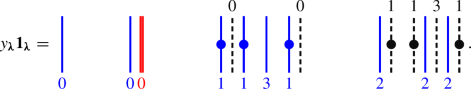
  One can check that it is not possible to pull any string in ${\textbf {1}} _{{\varvec{\lambda }}}$ further to the right. For type $C^{(1)}_{4}$ we have ${\text {res}}_{\rho }({\varvec{\lambda }})=(0,1,2,3,4,3,2,1,0)$, and we get:

  

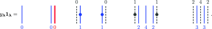
• (b) Let ${\varvec{\lambda }}=(5,5)$ for the quiver $C^{(1)}_{2}$. Then ${\text {res}}_{\rho }({\varvec{\lambda }})=(0,1,2,1,0,1,0,1,2,1)$ and the positioning function and the dot placement give:

  

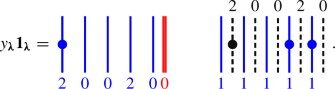
  The dotted idempotent in this case for the quiver $C^{(1)}_{3}$ is (with ${\text {res}}_{\rho }({\varvec{\lambda }})=(0,1,2,3,2,1,0,1,2,3)$)

  

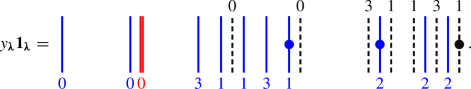
• (c) If ${\varvec{\lambda }}=(3,3,3)$ and we take the quiver $C^{(1)}_{2}$, then we get ${\text {res}}_{\rho }({\varvec{\lambda }})=(0,1,2,1,0,1,2,1,0)$ and:

  

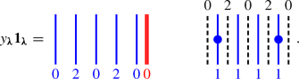
  Changing the quiver to $C^{(1)}_{3}$ gives the same residue sequence, but a different $y_{{\varvec{\lambda }}}{\textbf {1}} _{{\varvec{\lambda }}}$:

  

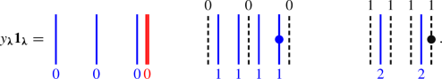
For readability, all diagrams are stretched in the x-direction because these diagrams tend to get cluttered. Note that this is the typical behavior: the $(e-2)$ and the e-strings always appear very close together because the $(e-1)$-strings does not have a ghost and the positioning function compensates for this by bouncing back, which interleaves these strings and their ghosts.

Remark 6B.4

The dotted idempotent $y_{{\varvec{\lambda }}}{\textbf {1}} _{{\varvec{\lambda }}}$ is not as complicated as the definition suggests. One first places the strings using the row reading order, following the rule that they are placed as far to the right as possible such that the previously placed ghost and strings stops the new strings being pulled further to the right. One then adds dots by looking at addable nodes. This is easy to feed into a machine and, in fact, the diagrams above are drawn by a TikZ macro that uses only the residue sequence. These macros are also available on GitHub [32].

Lemma 6B.5

Suppose that ${\varvec{\lambda }},{\varvec{\mu }}\in \underline{\textrm{P}}_{\underline{\ell },n}$. Then $y_{{\varvec{\lambda }}}{\textbf {1}} _{{\varvec{\lambda }}}=y_{{\varvec{\mu }}}{\textbf {1}} _{{\varvec{\mu }}}$ if and only if ${\varvec{\lambda }}={\varvec{\mu }}$.

Proof

If ${\text {res}}_{\rho }({\varvec{\lambda }})\ne {\text {res}}_{\rho }({\varvec{\mu }})$, then this is clear since ${\textbf {1}} _{{\varvec{\lambda }}}\ne {\textbf {1}} _{{\varvec{\mu }}}$ in this case. If ${\varvec{\lambda }}\ne {\varvec{\mu }}$ and ${\text {res}}_{\rho }({\varvec{\lambda }})={\text {res}}_{\rho }({\varvec{\mu }})$, then the polynomials $y_{{\varvec{\lambda }}}$ and $y_{{\varvec{\mu }}}$ are different by induction, so $y_{{\varvec{\lambda }}}{\textbf {1}} _{{\varvec{\lambda }}}\ne y_{{\varvec{\mu }}}{\textbf {1}} _{{\varvec{\mu }}}$ by Proposition 3B.12. $\square$

6.3 The homogeneous (affine) cellular basis of type C

For the algebra ${\mathscr {W}_{{\beta }}^{{\varvec{\rho }}}}(X)$ for type $C^{(1)}_{e}$ we will choose the Q-polynomials as in (2C.5).

Define $\underline{\textrm{P}}_{\underline{\ell },n}$ and X exactly as in Definition 5A.15 and consider the weighted KLRW algebra ${\mathscr {W}_{{\beta }}^{{\varvec{\rho }}}}(X)$ of type $C^{(1)}_{\ell }$. Repeating Definition 5A.19, define the set ${\hbox {SStd}_{{\varvec{\kappa }}}}({\varvec{\lambda }},{\varvec{\mu }})$ of semistandard ${\varvec{\lambda }}$-tableaux of type ${\varvec{\mu }}$ using the type C positioning function above. Set ${\hbox {SStd}_{{\varvec{\kappa }}}}({\varvec{\lambda }})=\bigcup _{{\varvec{\mu }}}{\hbox {SStd}_{{\varvec{\kappa }}}}({\varvec{\lambda }},{\varvec{\mu }})$. As for type A, $({}_{-})^{\star }$ is the antiinvolution from (3A.2), which we will use from now on. As in Definition 5A.21, define diagrams $D_{{\varvec{S}}}$ and $D_{{\varvec{T}}}$ for ${\varvec{S}},{\varvec{T}}\in {\text {Std}}({\varvec{\lambda }},{\varvec{\mu }})$. Given ${\varvec{a}}\in \mathbb {Z}^{n}$ define $D_{{\varvec{S}}{\varvec{T}}}^{{\varvec{a}}}=D_{{\varvec{S}}}^{\star }y^{{\varvec{a}}}y_{{\varvec{\lambda }}}{\textbf {1}} _{{\varvec{\lambda }}}D_{{\varvec{T}}}$. For ${\varvec{a}}=(0,\ldots ,0)$ set $D_{{\varvec{S}}{\varvec{T}}}=D_{{\varvec{S}}{\varvec{T}}}^{{\varvec{a}}}$.

The definition of the diagrams $D_{{\varvec{S}}{\varvec{T}}}$ is almost exactly the same as in type A except that $y_{{\varvec{\lambda }}}$ appears on their equator and we are using a different choice of positioning function. Recall the definition of the set $A^{\underline{{\varvec{\kappa }}}}({\varvec{\lambda }})$ from Sect. 5B.

Definition 6C.1

Let ${\varvec{\lambda }},{\varvec{\mu }}\in \underline{\textrm{P}}_{\underline{\ell },n}$. Then ${\varvec{\lambda }}$ dominates ${\varvec{\mu }}$, written ${\varvec{\lambda }}\trianglerighteq _{C}{\varvec{\mu }}$, if there exists a bijection $d:{\varvec{\lambda }}\rightarrow {\varvec{\mu }}$ such that $\texttt {x} _{\underline{{\varvec{\kappa }}}}^{C}(\alpha )\ge \texttt {x} _{\underline{{\varvec{\kappa }}}}^{C}\big (d(\alpha )\big )$ and the solid string in ${\textbf {1}} _{{\varvec{\lambda }}}$ at position $\texttt {x} _{\underline{{\varvec{\kappa }}}}^{C}(\alpha )$ has at least as many dots as the solid string in ${\textbf {1}} _{{\varvec{\mu }}}$ at position $\texttt {x} _{\underline{{\varvec{\kappa }}}}^{C}\big (d(\alpha )\big )$, for all $\alpha \in {\varvec{\lambda }}$. Write ${\varvec{\lambda }}\vartriangleright _{C}{\varvec{\mu }}$ if ${\varvec{\lambda }}\trianglerighteq _{C}{\varvec{\mu }}$ and ${\varvec{\lambda }}\ne {\varvec{\mu }}$.

Remark 6C.2

As in type A, it is not clear to the authors how the partial order $\vartriangleright _{C}$ compares with the dominance order on partitions, which is used in [7] or [14].

Throughout this section we consider $\underline{\textrm{P}}_{\underline{\ell },n}$ as a poset ordered by $\trianglelefteq _{C}$. In particular, we use Definition 6C.1 as the partial order in the following theorem. As in type $A^{(1)}_{e}$ we define $\deg {\varvec{S}}=\deg D_{{\varvec{S}}}$, $\deg {\varvec{a}}=\deg y^{{\varvec{a}}}{\textbf {1}} _{{\varvec{\lambda }}}$ and $\deg {\varvec{T}}=\deg D_{{\varvec{T}}}$.

Theorem 6C.3

The set $\textrm{B}_{\mathscr {W}}=\{ D_{{\varvec{S}}{\varvec{T}}}^{\varvec{a}}|{\varvec{\lambda }}\in \underline{\textrm{P}}_{\underline{\ell },n},{\varvec{S}},{\varvec{T}}\in {\hbox {SStd}_{{\varvec{\kappa }}}}({\varvec{\lambda }}),{\varvec{a}}\in A^{\underline{{\varvec{\kappa }}}}({\varvec{\lambda }})\}$ is a homogeneous affine cellular basis of ${\mathscr {W}_{n}^{{\varvec{\rho }}}}(X)$ with respect to the poset $(\underline{\textrm{P}}_{\underline{\ell },n},\trianglelefteq _{C})$.

The proof follows the same road as the proof of Theorem 5B.7, see Sect. 6E below.

As before we immediately obtain:

Corollary 6C.4

The set $\textrm{B}_{\mathscr {R}}=\{D_{{\varvec{S}}{\varvec{T}}}|{\varvec{\lambda }}\in \textrm{P}_{\ell ,n},{\varvec{S}},{\varvec{T}}\in {\hbox {SStd}_{{\varvec{\kappa }}}}({\varvec{\lambda }})\}$ is a homogeneous cellular basis of the cyclotomic weighted KLRW algebra ${\mathscr {R}_{n}^{{\varvec{\rho }}}}(X)$.

Giving a basis for the KLR algebra of type $C^{(1)}_{e}$ requires some additional notation. Recall from Sect. 5B that ${\varvec{\omega }}=(1^{n}|0|\ldots |0)$. By definition, ${\varvec{\omega }}\trianglelefteq _{C}{\varvec{\lambda }}$, for all ${\varvec{\lambda }}\in \underline{\textrm{P}}_{\underline{\ell },n}$. Recall from (5B.9) that ${\textbf {1}} _{A,n}$ is the sum of diagrams with positions given by ${\varvec{\omega }}$, where the sum is over all residues. Similarly, define

That is, ${\textbf {1}} _{C,n}$ is the sum of straight line diagrams connecting the type A coordinates and type C coordinates for ${\varvec{\omega }}$, where the sum is over all residues $\textbf{i}\in I^{n}$. Then ${\textbf {1}} _{C,n}^{\star }{\mathscr {W}_{{\beta }}^{{\varvec{\rho }}}}(X){\textbf {1}} _{C,n}\cong \mathcal {W}_{{\beta }}^{{{\varvec{\rho }}}}$ exactly as in Corollary 5B.10, and we also have ${\textbf {1}} _{C,n}^{\star }{\mathscr {R}_{{\beta }}^{{\varvec{\rho }}}}(X){\textbf {1}} _{C,n}\cong \mathcal {R}_{{\beta }}^{{{\varvec{\rho }}}}$. We identify the corresponding algebras.

As in type A, a standard tableau is a semistandard tableau of type ${\varvec{\omega }}$. Let ${\text {Std}}({\varvec{\lambda }})$ be the set of standard tableaux of shape ${\varvec{\lambda }}$, for ${\varvec{\lambda }}\in \underline{\textrm{P}}_{\underline{\ell },n}$. For $\varvec{s},\varvec{t}\in {\text {Std}}({\varvec{\lambda }})$ and ${\varvec{a}}\in A^{\underline{{\varvec{\kappa }}}}({\varvec{\lambda }})$ set $E^{{\varvec{a}}}_{\varvec{s}\varvec{t}}={\textbf {1}} _{C,n}^{\star }D^{{\varvec{a}}}_{\varvec{s}\varvec{t}}{\textbf {1}} _{C,n}$ and let $E_{\varvec{s}\varvec{t}}=E^{(0,\ldots ,0)}_{\varvec{s}\varvec{t}}$.

Proposition 6C.6

The set $\textrm{B}_{\mathcal {W}}=\{E^{{\varvec{a}}}_{\varvec{s}\varvec{t}}|{\varvec{\lambda }}\in \textrm{P}_{\ell ,n},\varvec{s},\varvec{t}\in {\text {Std}}({\varvec{\lambda }}),{\varvec{a}}\in A^{\underline{{\varvec{\kappa }}}}({\varvec{\lambda }})\}$ is a homogeneous affine cellular basis of $\mathcal {W}_{{\beta }}^{{{\varvec{\rho }}}}$ and $\textrm{B}_{\mathcal {R}}=\{E_{\varvec{s}\varvec{t}}|{\varvec{\lambda }}\in \textrm{P}_{\ell ,n},\varvec{s},\varvec{t}\in {\text {Std}}({\varvec{\lambda }})\}$ is a homogeneous cellular basis of $\mathcal {R}_{{\beta }}^{{{\varvec{\rho }}}}$.

Proof

As noted above, the argument of Proposition 3F.1 shows that $\mathcal {W}_{{\beta }}^{{{\varvec{\rho }}}}\cong {\textbf {1}} _{C,n}^{\star }{\mathscr {W}_{{\beta }}^{{\varvec{\rho }}}}(X){\textbf {1}} _{C,n}$. We claim that $\mathcal {W}_{{\beta }}^{{{\varvec{\rho }}}}\cong {\textbf {1}} _{C,n}^{\star }{\mathscr {W}_{{\beta }}^{{\varvec{\rho }}}}(X){\textbf {1}} _{C,n}$. The evident conjugation map $\mathcal {W}_{{\beta }}^{{{\varvec{\rho }}}}\rightarrow {\textbf {1}} _{C,n}^{\star }{\mathscr {W}_{{\beta }}^{{\varvec{\rho }}}}(X){\textbf {1}} _{C,n}$ identifies the polynomial bases of Proposition 3B.12 on both sides, and so it is an isomorphism. By Theorem 6C.3, $\{ D^{{\varvec{a}}}_{\varvec{s}\varvec{t}}\}$ is a basis of ${\textbf {1}} _{C,n}^{\star }{\mathscr {W}_{{\beta }}^{{\varvec{\rho }}}}(X){\textbf {1}} _{C,n}$ so $\{ E^{{\varvec{a}}}_{\varvec{s}\varvec{t}}\}$ is a basis of $\mathcal {W}_{{\beta }}^{{{\varvec{\rho }}}}$. The unsteady basis elements are identified under this isomorphism, so we also get $\mathcal {R}_{{\beta }}^{{{\varvec{\rho }}}}\cong {\textbf {1}} _{C,n}^{\star }{\mathscr {R}_{{\beta }}^{{\varvec{\rho }}}}(X){\textbf {1}} _{C,n}$, which finishes the proof. $\square$

As in type A, as a corollary we obtain dimension formulas for the cyclotomic KLRW and KLR algebras that are similar to (5B.12). For the cyclotomic KLR algebras this recovers [7, Theorem 2.5].

Remark 6C.7

As in (5B.13), Proposition 6C.6 constructs a basis of the KLR algebras of type $C^{(1)}_{e}$ for each choice of loading. A basis for the cyclotomic KLR algebras of type $C^{(1)}_{e}$ is constructed in [14] but it is not clear to the authors how the basis in [14] is related to the basis in Proposition 6C.6 because, at first sight, they use different partial orders. This is slightly surprising because the definition of the basis in Proposition 6C.6 was partly motivated by [14].

6.4 Some results regarding simple modules

Classifying the simple ${\mathscr {W}_{{\beta }}^{{\varvec{\rho }}}}(X)$ and ${\mathscr {R}_{{\beta }}^{{\varvec{\rho }}}}(X)$ modules in type C is more involved than in type A, which was discussed in Sect. 5C. More precisely, most of Sect. 5C goes through without change with the crucial difference being that Theorem 5C.1 because it is not clear when pairing on $\Delta ({\varvec{\lambda }},K)$ can be zero. We are only able to show that the cellular pairing is nonzero for the $\underline{\ell }$-partitions $\underline{\textrm{P}}_{\underline{\ell },n}^{g}$, that we now define.

Definition 6D.1

Let $\underline{\textrm{P}}_{\underline{\ell },n}^{g}\subset \underline{\textrm{P}}_{\underline{\ell },n}$ be the subset of all $\underline{\ell }$-partitions ${\varvec{\lambda }}$ such that $y_{{\varvec{\lambda }}}{\textbf {1}} _{{\varvec{\lambda }}}$ has no dots or each dotted i-string is locally of the form:

and the illustrated strings can be pulled arbitrarily close to one another. In particular, there are no multilocal configurations stopping a naive isotopy.

Example 6D.2

We ignore the affine part in this example. For type $C^{(1)}_{3}$, $n=5$, $\ell =1$ and ${\varvec{\rho }}=(0)$ we have seven 1-partitions of five:

Hence, $\{ (3,1^{2}),(2^{2},1),(2,1^{3}),(1^{5})\}=\textrm{P}_{{\ell },n}^{g}$ in this case.

With the same notions as in type A, the (much weaker) analog of Theorem 5C.1 reads:

Proposition 6D.3

Suppose that R is a field.

• (a) The set $\{ L({\varvec{\lambda }},K)|{\varvec{\lambda }}\in \underline{\textrm{P}}_{\underline{\ell },n}^{g}\text { and }K\in S\big (B({\varvec{\lambda }})\big )\}$ is a non-redundant set of simple ${\mathscr {W}_{n}^{{\varvec{\rho }}}}(X)$-modules.

• (b) The set $\{ q^{s}L({\varvec{\lambda }})|{\varvec{\lambda }}\in \underline{\textrm{P}}_{\underline{\ell },n}^{g}\text { and }s\in \mathbb {Z}\}$ is a non-redundant set of graded simple ${\mathscr {W}_{n}^{{\varvec{\rho }}}}(X)$-modules.

• (c) The set $\{ L({\varvec{\lambda }})|{\varvec{\lambda }}\in \textrm{P}_{{\ell },n}^{g}\}$ is a non-redundant set of simple ${\mathscr {R}_{n}^{{\varvec{\rho }}}}(X)$-modules.

• (d) The set $\{ q^{s}L({\varvec{\lambda }})|{\varvec{\lambda }}\in \textrm{P}_{{\ell },n}^{g}\text { and }s\in \mathbb {Z}\}$ is a non-redundant set of graded simple ${\mathscr {R}_{n}^{{\varvec{\rho }}}}(X)$-modules.

Proof

In type A, the proof of Theorem 5C.1 shows that because every ${\varvec{\lambda }}\in \underline{\textrm{P}}_{\underline{\ell },n}$ has an associated idempotent the cellular pairing is nonzero. We argue in the same way for ${\varvec{\lambda }}\in \underline{\textrm{P}}_{\underline{\ell },n}^{g}$. If $y_{{\varvec{\lambda }}}{\textbf {1}} _{{\varvec{\lambda }}}$ has no dots, then $y_{{\varvec{\lambda }}}{\textbf {1}} _{{\varvec{\lambda }}}={\textbf {1}} _{{\varvec{\lambda }}}$ is an idempotent and as before $L({\varvec{\lambda }})\ne 0$. Otherwise, if only the first condition in Definition 6D.1 appears for $y_{{\varvec{\lambda }}}{\textbf {1}} _{{\varvec{\lambda }}}$, then our construction of the basis elements $D^{{\varvec{a}}}_{\varvec{s}\varvec{t}}$ implies that we get idempotents that are locally of the form

That these diagrams are indeed idempotents follows from (2C.8). In all other situations we first use (5D.6). Note that in both of the right-hand diagrams in (5D.6) we have locally

so these summands secretly contain idempotents by (2C.8). This implies that the cellular pairing is nonzero in these cases, so the associated simple modules are nonzero. The general theory of cellular algebras then implies that they are pairwise non-isomorphic, so this completes the proof. $\square$

Remark 6D.4

In small examples, if ${\varvec{\lambda }}\in \textrm{P}_{{\ell },n}^{g}$, then the corresponding simple module of the KLR algebra $\mathcal {W}_{{\beta }}^{{{\varvec{\rho }}}}$ is nonzero, although not all simple modules arise in this way. This is consistent with [43, Corollary 2.16], which claims that ${\mathscr {R}_{{\beta }}^{{\varvec{\rho }}}}(X)$ is Morita equivalent to $\mathcal {W}_{{\beta }}^{{{\varvec{\rho }}}}$.

The analog of Corollary 5C.2 fails in type $C^{(1)}_{e}$:

Proposition 6D.5

Suppose that R is a field. The algebra ${\mathscr {W}_{{\beta }}^{{\varvec{\rho }}}}(X)$ is not a graded affine quasi-hereditary algebra and ${\mathscr {R}_{{\beta }}^{{\varvec{\rho }}}}(X)$ is not a graded quasi-hereditary algebra.

Proof

The cell modules for $\underline{\ell }$-partitions with a component of the form (n) are one dimensional and concentrated in strictly positive degree, so they cannot carry a simple module. Hence, these algebras cannot be quasi-hereditary by the general theory of cellular algebras; cf. [27, Theorem 4.1]. $\square$

6.5 Proof of cellularity in type C

Most of the arguments that we use to prove Theorem 6C.3 are the same as those in type A, for example Lemma 5D.1 holds without change, and we focus on the differences. Recall that the Q-polynomials for type C that we use are the ones in (2C.5). We have the following analog of Lemma 5D.4. The proof is the same as the one for Lemma 5D.4 but taking the changed Q-polynomials into account.

Lemma 6E.1

The relations in (5D.5) hold unless (note that there are no ghost $(e-1)$-strings):

where the ghost i-string should be ignored in these diagrams when $i=e-1$. Moreover, (5D.6) holds (deleting ghost $(e-1)$-strings if necessary) unless:

As usual, we pull the green strings, or the dot on the green strings, to the right.

Proof

These follow using similar arguments to those in Lemma 5D.4. $\square$

Remark 6E.3

In contrast to type $A^{(1)}_{e}$, relation (6E.2) does not allow any strings to be pulled further to the right for the configurations

This is the reason why (6A.9) are minimal configurations.

A dotted straight line diagram is a diagram of the form $y_{1}^{a_{1}}\ldots y_{n}^{a_{n}}S$, where S is a straight line diagram and $a_{k}\in \{ 0,1\}$ for $1\le k\le n$. (Note that there is at most one dot per string.)

We need a type C version of Lemma 5D.16, for which we need analogs of Young equivalence classes.

In type A, Young equivalence classes of strings were defined using adjacency. In type C, we define Young equivalence classes using “closeness” of strings. In a dotted straight line diagram two strings are close if we can pull them arbitrarily close to one another in a neighborhood that does not contain any other strings using only (multilocal) isotopies. Note that two solid strings can be adjacent without being close because their ghost strings can prevent them from being pulled arbitrarily close together. We use close and to the left/right in the evident way.

Example 6E.4

In contrast to being adjacent, the property of being close is multilocal. For example, in (5D.13) only the left diagram has a solid i-string that is close to a solid j-string.

For $i,j\in I$, a close triple of the form (i, j, i) is a collection of three strings of the form

that are all close to their direct neighbors. Next, motivated by (6A.10) we define:

Definition 6E.5

Let S be a dotted straight line diagram. Fix $k\in I$. Solid i and j-strings of S are k-row equivalent if the i-string carries a dot if and only if $i=k$, and either:

• (a) $0\le i<e-1$, $j=i+1$ and the ghost i-string is close and to the right of the solid $(i+1)$-string;

• (b) $i=e$, $j=e-1$ and the ghost e-string is close and to the right of the solid $(e-1)$-string;

• (c) $0<i<e$, $j=i-1$ and the solid i-string is close and to the right of the ghost $(i-1)$-string;

• (d) $i=e-1$, $j=e$ and the solid $(e-1)$-string is close and to the right of the ghost e-string.

A k-row equivalence class is admissible if all close triples in the equivalence class are of the form (1, 0, 1) or $(e-1,e,e-1)$.

When we apply Definition 6E.5, if the i-string corresponds to a node (m, r, c), then $k={\text {res}}_{\rho }(m,r+1,1)$ is the residue of the first now in the next row, as in (6A.10).

By definition, the strings in a k-row equivalence class are ordered by closeness, starting with a string that is not close and to the right of any other in the same class. Hence, we can refer to the first and last strings in a row equivalence class. Recall the function $\textsf{r}\,{:}\,\mathbb {Z}\!\longrightarrow \!I$ from (6A.1).

Definition 6E.6

A Young equivalence class Y of solid strings in S is a disjoint union of admissible k-row equivalence classes, $R_{1}\cup \ldots \cup R_{z}$ where $R_{a}$ is a $k_{a}$-row equivalence class, such that:

• (a) The first string in $R_{1}$ has residue $i=\textsf{r}(k_{1}+1)$ and is close to an (affine) red i-string;

• (b) $|R_{1}|\ge |R_{2}|\ge \ldots \ge |R_{z}|$;

• (c) $k_{a+1}=\textsf{r}(k_{a}-1)$ and the first string in $R_{a+1}$ is a $\textsf{r}(k_{a})$-string and close to a dotted string of the same residue in $R_{a}$, or there is a j-string in $R_{a}$ that satisfies one of conditions (a)–(d) in Definition 6E.5 with respect to this string.

Remark 6E.7

As in type A, Definition 6E.6 is motivated by the box configurations in (6A.7)

As in Lemma 5D.9, let L(S) be the left justification of a (dotted) straight line diagram, defined with respect to the dominance order $\vartriangleright _{C}$. Note that not all solid strings in a dotted straight line diagram necessarily belong to a Young equivalence class, as implied, for example, by Definition 6E.6(a). Instead, we have:

Lemma 6E.8

Let S be a dotted straight line diagram. Then $L(S)=L(y_{{\varvec{\lambda }}}{\textbf {1}} _{{\varvec{\lambda }}})$, for some ${\varvec{\lambda }}\in \underline{\textrm{P}}_{\underline{\ell },n}$, if and only if every solid string in S belongs to a Young equivalence class.

Proof

The dotted straight line diagram $y_{{\varvec{\lambda }}}{\textbf {1}} _{{\varvec{\lambda }}}$ is constructed by reading along the rows of the components of ${\varvec{\lambda }}$. By Definition 6E.5, (6A.7) and Definition 6B.1, the solid strings corresponding to nodes in the same row of ${\varvec{\lambda }}$ are k-row equivalent (where k is the residue of the first node in the row below the one that defines the equivalence) and the strings corresponding to the component $\lambda ^{(m)}$ are Young equivalent. Hence, each solid string in $y_{{\varvec{\lambda }}}{\textbf {1}} _{{\varvec{\lambda }}}$ belongs to a Young equivalence class.

Conversely, suppose that S is a dotted straight line diagram and that the solid strings in S are a disjoint union of Young equivalence classes. Let Y be a Young equivalence class of solid strings in S. As in Lemma 5D.16 we inductively associate the solid strings in Y with a $\underline{\ell }$-partition ${\varvec{\lambda }}$. By Definition 6E.6.(a), the first string of Y is left adjacent to an (affine) red string of the same residue. If this is the mth red string, then identify the solid string with the node (m, 1, 1). By induction, suppose that the solid i-string corresponds to the node $(m,r,c)\in {\varvec{\lambda }}$.

First suppose that this i-string is not the last solid string in its row equivalence class then, in view of (6A.7), conditions (a)–(d) in Definition 6E.5 ensure that the next solid j-string corresponds to the node $(m,r,c+1)$. Furthermore, ${\text {res}}_{\rho }(m,r,c+1)=j$ since the row equivalence classes are admissible. By Definition 6E.6.(b), ${\varvec{\lambda }}\cup \{ (m,r,c+1)\}$ is still of $\underline{\ell }$-partition shape.

Finally, suppose that the i-string is the last string in its row equivalence class $R_{a}$ consider the j-string that is the first string in $R_{a+1}$. The two residue conditions in Definition 6E.6.(c) ensure that $(m,r+1,1)$ is an addable j-node of ${\varvec{\lambda }}$. It remains to observe that the closeness requirements in Definition 6E.6.(c) correspond to the string configurations of (6A.10). $\square$

Proposition 6E.9

Suppose that $D\in {\mathscr {W}_{n}^{{\varvec{\rho }}}}(X)$ and that D factors through the dotted idempotent diagram S. Then there exists ${\varvec{\lambda }}\in \underline{\textrm{P}}_{\underline{\ell },n}$ such that D factors through $y_{{\varvec{\lambda }}}{\textbf {1}} _{{\varvec{\lambda }}}$ and $L(S)\trianglelefteq _{C}{\varvec{\lambda }}$.

The proof of Proposition 6E.9 is similar to the proof of Proposition 5D.17.

Proof

It is enough to show that S factors through $y_{{\varvec{\lambda }}}{\textbf {1}} _{{\varvec{\lambda }}}$ for some ${\varvec{\lambda }}\in \underline{\textrm{P}}_{\underline{\ell },n}$. If S satisfies the conditions of Lemma 6E.8, then $S=y_{{\varvec{\lambda }}}{\textbf {1}} _{{\varvec{\lambda }}}$ for some ${\varvec{\lambda }}\in \underline{\textrm{P}}_{\underline{\ell },n}$, so the proposition follows. Hence, we can assume that the solid strings in S do not form a disjoint union of Young equivalence classes.

Take the rightmost solid string not in any Young equivalence class, call it s. We proceed with a case-by-case check. There are now six cases to consider.

Case 1. First, if there is no string close and to the right of s, or its ghost, then we could pull s arbitrarily far to the right. So, we can assume that this string is left adjacent to an affine red string of the same residue.

Hence, we are reduced to considering the case where s is close and to the left of a solid or ghost string t. We claim that we can pull s rightwards or link it to the Young equivalence class of t, if applicable. Below we assume that s is close to t. The case where the ghost of s is close to t can be treated mutatis mutandis.

Case 2. First assume that s is not in the Young equivalence class of t because the admissibility condition on close triples is violated. In this situation we can either apply a Reidemeister II relation to pull s further rightwards, or apply (5D.6) together with (5D.3) to jump the dot.

Case 3. We now assume that s is not in the Young equivalence class of t because Definition 6E.6.(b) is violated. If the row equivalence class of t does not contain an earlier string of the same residue as s, then we are in the situation illustrated in (6A.11). In this case we can apply either (5D.6) or (6E.2) (note that if $i\pm 1\in \{ 0,e\}$ in leftmost string so (6E.2) applies), to pull s further to the right. Note that this is the only situation where this could happen. To see this consider

Note that there are four subcases here since the residues could be either increasing or decreasing as we read down the first column or along this row. In the case of the diagram on the right, if necessary we iterate this process to move the nodes as low as possible in the component so that the corresponding dotted idempotent does not require additional dots. Hence, in all cases, S factors through a more dominant dotted idempotent diagram.

We now assume that we are not in Cases 1, 2 and 3.

Case 4. If t is an (affine) red string, then it has to have a different residue to s by Definition 6E.6.(a). In this case, a standard Reidemeister II relation applies and we can move s rightwards.

Case 5. If t is a solid string, then the only situations preventing us from pulling s rightwards via a Reidemeister II relation are the ones displayed in (5D.2) and (5D.3). In both cases we can pull s rightwards except for the diagram to the right of the equals sign in (5D.3). However, for this diagram we observe that either s and t are in the same Young equivalence class by Definition 6E.6.(c), or t is now the rightmost solid string that is not in any Young equivalence class. Note that it can happen that t is no longer contained in a Young equivalence class because the dot has moved onto t. As s and t are row equivalence by repeating the argument applied to t sufficiently many times shows that s (and t), belong to a Young equivalence class.

Case 6. Assume that t is a ghost string. Note that we are not in the situations of (c) and (d) of Definition 6E.5 because, by assumption, s is rightmost with respect to being not in any Young equivalence class. Hence, a Reidemeister II relation applies.

Note that after pulling s rightwards it is either contained in a Young equivalence class (cases 1, 2, 3 or 5) or we can continue pulling it two the right (cases 4 and 6). Repeating the argument sufficiently many times shows that s is contained in a Young equivalence class because we cannot pull s arbitrarily far to the right as it will eventually stop next to an (affine) red string of the same residue. Hence, the result follows by induction. $\square$

We again simplify notation and write $\vartriangleright =\vartriangleright _{C}$.

Lemma 6E.10

Suppose that ${\varvec{\lambda }}\in \textrm{P}_{\ell ,n}$ and $1\le m\le n$ satisfies $\texttt {x} _{\underline{{\varvec{\kappa }}}}^{C}({\varvec{\lambda }})_{m}\le \texttt {x} _{\underline{{\varvec{\kappa }}}}^{C}(\ell ,1,n)$. Then .

Proof

The proof is essentially the same as Lemma 5D.18. Suppose that the mth string is an i-string. By Lemma 6E.8 and Definition 6B.1, $y_{m}y_{{\varvec{\lambda }}}{\textbf {1}} _{{\varvec{\lambda }}}$ is a dotted idempotent diagram if and only if $y_{m}y_{{\varvec{\lambda }}}{\textbf {1}} _{{\varvec{\lambda }}}=y_{{\varvec{\mu }}}{\textbf {1}} _{{\varvec{\mu }}}$ for some $\underline{\ell }$-partition ${\varvec{\mu }}$ with ${\varvec{\mu }}\vartriangleright _{C}{\varvec{\lambda }}$. If $y_{m}y_{{\varvec{\lambda }}}{\textbf {1}} _{{\varvec{\lambda }}}$ is not a dotted straight line diagram, then, by Proposition 6E.9, it factors through a dotted straight line diagram $y_{{\varvec{\mu }}}{\textbf {1}} _{{\varvec{\mu }}}$, for some $\underline{\ell }$-partition ${\varvec{\mu }}$ with ${\varvec{\mu }}\vartriangleright _{C}{\varvec{\lambda }}$. So , as required. $\square$

For $w\in {\mathfrak {S}_{n}}$ and ${\varvec{\lambda }}\in \underline{\textrm{P}}_{\underline{\ell },n}$ define the diagram $D_{{\varvec{\lambda }}}(w)=D(w){\textbf {1}} _{{\varvec{\lambda }}}$ as in Sect. 5D.

Lemma 6E.11

Suppose that ${\varvec{\lambda }}\in \underline{\textrm{P}}_{\underline{\ell },n}$ and $w\in {\mathfrak {S}_{{\varvec{\lambda }}}}$. Then .

Proof

This follows by repeating the argument of Lemma 5D.19. $\square$

Proof of Theorem 6C.3

Using Proposition 6E.9 and the last two lemmas, the (completely formal) argument of Proposition 5D.20 shows that ${\mathscr {W}_{{\beta }}^{{\varvec{\rho }}}}(X)$ is spanned by the elements in the statement of Theorem 6C.3. Similarly, linear independence and cellularity follow exactly as in the proof of Theorem 5B.7. Note that the argument for linear independence relies on the faithful module in Proposition 3B.12, which is valid in any type, whilst the proof of cellularity is a purely formal argument using Proposition 6E.9, Lemma 6E.10 and Lemma 6E.11.

7 Table of notation and central concepts

The following is the list of the most important concepts in this paper.

Name	Symbol	Description
The quiver	$\Gamma =(I,E)$, $i\rightarrow j$, $i\Rightarrow j$, $i\Rrightarrow j$ and $i\rightsquigarrow j$ (multiplicity is unimportant)	The quiver and its various edges, see Sect. 2A
$\ell$=level, ${\varvec{\kappa }}$=charge	n, $\ell$, e, ${\varvec{\kappa }}$, ${\varvec{\rho }}$, X, ${\varvec{\sigma }}$	The number of solid strings, the number of red strings, the number of vertices in the quiver, the positions of the red strings, the labels of the red strings, the positions and labels of the solid strings, the ghost shift; all of these are fixed from the start, see Sect. 2
Solid, ghost, red and affine strings		Strings in diagrams, see Sect. 2B
The infinitesimal and the asymptotic case	No specific symbol	The infinitesimal case, where ${\varvec{\sigma }}=(\varepsilon ,\ldots ,\varepsilon )$, and the asymptotic case, where ${\varvec{\sigma }}=(1/\varepsilon ,\ldots ,1/\varepsilon )$, both for $0<\varepsilon \ll 1$, see Sect. 2B
Q-polynomials and algebraic dots	$Q_{ij}(u,v)$, $Q_{ijk}(u,v,w)$, $y_{i}$	The Q-polynomials, see (2C.5), and variables that act as dots
Affine notation	$\underline{\ell }$, $\underline{{\varvec{\kappa }}}$, $\underline{{\varvec{\rho }}}$	We set $\underline{\ell }=\ell +n(e+1)$. These ensure that we have enough affine red string to catch every solid string, see Sect. 5A
Weighted KLRW algebra	${\mathscr {W}_{n}^{{\varvec{\rho }}}}(X)$	A diagram algebra with n solid strings (sometimes we use this with a $\beta \in Q^{+}$) with top and bottom x-coordinates in X, see Sect. 2C
The cyclotomic version	${\mathscr {R}_{n}^{{\varvec{\rho }}}}(X)$	A quotient of ${\mathscr {W}_{n}^{{\varvec{\rho }}}}(X)$, cf. Sect. 3D
Antiinvolution	$({}_{-}){}^{\star }$	The antiinvolution mirrors diagrams in a horizontal axis, see Sect. 3A
Idempotent diagram for $(\varvec{x},\textbf{i})$ or ${\varvec{\lambda }}$	${\textbf {1}} _{\varvec{x},\textbf{i}}$, ${\textbf {1}} _{{\varvec{\lambda }}}$	The idempotent diagram created by inductively placing strings while reading along the rows of the $\underline{{\varvec{\rho }}}$-partition ${\varvec{\lambda }}$, see Sect. 5A
Truncation idempotents	${\textbf {1}} _{A,n}$, ${\textbf {1}} _{C,n}$	The idempotent diagrams for truncation to the KLR(W) algebras, see (5B.9) and (6C.5)
Permutation diagram for $w\in {\mathfrak {S}_{n}}$ or ${\varvec{S}}$	$D_{w}$, $D_{{\varvec{S}}}$	A permutation diagram associated to, for example, the $\underline{{\varvec{\rho }}}$-tableaux ${\varvec{S}}$, see Sect. 5A
KLRW and its cyclotomic quotient	${{\mathcal {W}}_{n}^{{{\varvec{\rho }}}}}$, ${{\mathcal {R}}_{n}^{{{\varvec{\rho }}}}}$	The ‘classical’ KLRW algebras, see Sect. 3F
Notation for subdivision	$\overline{{}_{-}}$	Everything related to the subdivision is overlined in Sect. 4
Partitions	$\underline{\textrm{P}}_{\underline{\ell },n}$, $\textrm{P}_{\ell ,n}$	Indexing sets for the middle of the cellular bases of ${\mathscr {W}_{n}^{{\varvec{\rho }}}}(X)$ and ${\mathscr {R}_{n}^{{\varvec{\rho }}}}(X)$, see Sect. 5B

Name	Symbol	Description
Nodes	(m, r, c)	Nodes in (shifted) partitions: m is the component index, r the row index and c the column index, see Sect. 5B
Positioning function	$\texttt {x} _{\underline{{\varvec{\kappa }}}}^{A}(m,r,c), \texttt {x} _{\underline{{\varvec{\kappa }}}}^{C}(m,r,c)$	The functions (in types A and C) that give the x-coordinates of solid strings, see Sect. 5A
Cellular basis elements	$D_{{\varvec{S}}{\varvec{T}}}^{{\varvec{a}}}$, $D_{{\varvec{S}}{\varvec{T}}}$	The homogeneous cellular basis elements, see Sect. 5B, for ${\mathscr {W}_{n}^{{\varvec{\rho }}}}(X)$ and ${\mathscr {R}_{n}^{{\varvec{\rho }}}}(X)$
Cellular basis sets	$\textrm{B}_{\mathscr {W}}$, $\textrm{B}_{\mathscr {R}}$	The homogeneous cellular bases sets, see Sect. 5B, for ${\mathscr {W}_{n}^{{\varvec{\rho }}}}(X)$ and ${\mathscr {R}_{n}^{{\varvec{\rho }}}}(X)$
Cellular order	$\trianglelefteq _{A}$, $\trianglelefteq _{C}$	The cellular orders (type A and C) measuring how far strings are to the right, see Sect. 5B
(Affine) cell and simple modules	$\Delta ({\varvec{\lambda }},K)$, $\Delta ({\varvec{\lambda }})$, and $L({\varvec{\lambda }},K)$, $L({\varvec{\lambda }})$	The cell modules coming for the cellular structure and their associated simple modules, see Sect. 5C

References

Allcock, D.: Braid pictures for Artin groups. Trans. Am. Math. Soc. 354(9), 3455–3474 (2002). https://doi.org/10.1090/S0002-9947-02-02944-6. arXiv:math/9907194
Ariki, S.: On the classification of simple modules for cyclotomic Hecke algebras of type \(G(m,1, n)\) and Kleshchev multipartitions. Osaka J. Math. 38(4), 827–837 (2001). arXiv:math/9908004
Ariki, S.: On cyclotomic quiver Hecke algebras of affine type. In: Ring Theory 2019. World Sci. Publ., Hackensack, pp. 3–22 (2021). https://doi.org/10.1142/9789811230295_0001
Ariki, S., Mathas, A.: The number of simple modules of the Hecke algebras of type \(G(r,1, n)\). Math. Z. 233(3), 601–623 (2000). https://doi.org/10.1007/s002090050489
Ariki, S., Park, E.: Representation type of finite quiver Hecke algebras of type \(A^{(2)}_{2\ell }\). J. Algebra 397, 457–488 (2014). https://doi.org/10.1016/j.jalgebra.2013.09.005. arXiv:1208.0889
Ariki, S., Park, E.: Representation type of finite quiver Hecke algebras of type \(D^{(2)}_{\ell +1}\). Trans. Am. Math. Soc. 368(5), 3211–3242 (2016). https://doi.org/10.1090/tran/6411. arXiv:1305.6367
Ariki, S., Park, E., Speyer, L.: Specht modules for quiver Hecke algebras of type \(C\). Publ. Res. Inst. Math. Sci. 55(3), 565–626 (2019). https://doi.org/10.4171/PRIMS/55-3-4. arXiv:1703.06425
Bowman, C.: The many integral graded cellular bases of Hecke algebras of complex reflection groups. Am. J. Math. 144(2), 437–504 (2022). https://doi.org/10.1353/ajm.2022.0008. arXiv:1702.06579
Brundan, J., Kleshchev, A.: Blocks of cyclotomic Hecke algebras and Khovanov-Lauda algebras. Invent. Math. 178(3), 451–484 (2009). https://doi.org/10.1007/s00222-009-0204-8. arXiv:0808.2032
Brundan, J., Kleshchev, A.: Graded decomposition numbers for cyclotomic Hecke algebras. Adv. Math. 222(6), 1883–1942 (2009). https://doi.org/10.1016/j.aim.2009.06.018. arXiv:0901.4450
Chuang, J., Miyachi, H.: Runner removal Morita equivalences. In: Representation Theory of Algebraic Groups and Quantum Groups, Volume 284 of Progr. Math., pp. 55–79. Birkhäuser/Springer, New York (2010). https://doi.org/10.1007/978-0-8176-4697-4_4
Cline, E., Parshall, B., Scott, L.: Finite-dimensional algebras and highest weight categories. J. Reine Angew. Math. 391, 85–99 (1988)
Ehrig, M., Tubbenhauer, D.: Relative cellular algebras. Transform. Groups 26(1), 229–277 (2021). https://doi.org/10.1007/S00031-019-09544-5. arXiv:1710.02851
Evseev, A., Mathas, A.: Content systems and deformations of cyclotomic KLR algebras of type \(A\) and \(C\). 2022. arXiv:2209.00134
Goodman, F.M., Graber, J.: Cellularity and the Jones basic construction. Adv. Appl. Math. 46(1–4), 312–362 (2011). https://doi.org/10.1016/j.aam.2010.10.003. arXiv:0906.1496
Graham, J.J., Lehrer, G.: Cellular algebras. Invent. Math. 123(1), 1–34 (1996). https://doi.org/10.1007/BF01232365
Hu, J., Mathas, A.: Graded cellular bases for the cyclotomic Khovanov–Lauda–Rouquier algebras of type \({A}\). Adv. Math. 225(2), 598–642 (2010). https://doi.org/10.1016/j.aim.2010.03.002. arXiv:0907.2985
Hu, J., Shi, L.: Graded dimensions and monomial bases for the cyclotomic quiver Hecke algebras (2021). Communications in Contemporary Mathematics, 2023 (to appear)
James, G., Mathas, A.: Equating decomposition numbers for different primes. J. Algebra 258(2), 599–614 (2002). https://doi.org/10.1016/S0021-8693(02)00644-0
Kac, V.G.: Infinite-Dimensional Lie Algebras, 3rd edn. Cambridge University Press, Cambridge (1990). https://doi.org/10.1017/CBO9780511626234
Khovanov, M., Lauda, A.D.: A diagrammatic approach to categorification of quantum groups I. Represent. Theory 13, 309–347 (2009). https://doi.org/10.1090/S1088-4165-09-00346-X. arXiv:0803.4121
Khovanov, M., Lauda, A.D.: A diagrammatic approach to categorification of quantum groups II. Trans. Am. Math. Soc. 363(5), 2685–2700 (2011). https://doi.org/10.1090/S0002-9947-2010-05210-9. arXiv:0804.2080
Kleshchev, A.S.: Affine highest weight categories and affine quasihereditary algebras. Proc. Lond. Math. Soc. (3) 110(4), 841–882 (2015). https://doi.org/10.1112/plms/pdv004. arXiv:1405.3328
Kleshchev, A.S., Loubert, J.W.: Affine cellularity of Khovanov–Lauda–Rouquier algebras of finite types. Int. Math. Res. Not. IMRN 14, 5659–5709 (2015). https://doi.org/10.1093/imrn/rnu096. arXiv:1310.4467
Kleshchev, A.S., Loubert, J.W., Miemietz, V.: Affine cellularity of Khovanov–Lauda–Rouquier algebras in type \(A\). J. Lond. Math. Soc. (2) 88(2), 338–358 (2013). https://doi.org/10.1112/jlms/jdt023. arXiv:1210.6542
König, S., Xi, C.: On the structure of cellular algebras. In: Algebras and Modules, II (Geiranger, 1996), Volume 24 of CMS Conf. Proc., pp. 365–386. Amer. Math. Soc., Providence (1998)
König, S., Xi, C.: Affine cellular algebras. Adv. Math. 229(1), 139–182 (2012). https://doi.org/10.1016/j.aim.2011.08.010
Lauda, A.D.: A categorification of quantum \({\rm sl}(2)\). Adv. Math. 225(6), 3327–3424 (2010). https://doi.org/10.1016/j.aim.2010.06.003. arXiv:0803.3652
Maksimau, R.: Categorical representations and KLR algebras. Algebra Numb. Theory 12(8), 1887–1921 (2018). https://doi.org/10.2140/ant.2018.12.1887. arXiv:1901.11026
Manivel, L.: Symmetric Functions, Schubert Polynomials and Degeneracy Loci, Volume 6 of SMF/AMS Texts and Monographs. American Mathematical Society, Providence; Société Mathématique de France, Paris, 2001. Translated from the 1998 French original by John R. Swallow, Cours Spécialisés [Specialized Courses], 3
Mathas, A.: Iwahori–Hecke Algebras and Schur Algebras of the Symmetric Group, Volume 15 of University Lecture Series. American Mathematical Society, Providence (1999). https://doi.org/10.1090/ulect/015
Mathas, A., Tubbenhauer, D.: SageMath code on GitHub to compute dimensions of cyclotomic KLR algebras; and Tikz macro on GitHub to display weighted KLRW idempotent diagrams (2022). https://github.com/dtubbenhauer/KLRWdimensions
Mathas, A., Tubbenhauer, D.: Cellularity for weighted KLRW algebras of types B, \(A^{(2)}\), \(D^{(2)}\). J. Lond. Math. Soc. (2) 107(3), 1002–1044 (2023). https://doi.org/10.1112/jlms.12706. arXiv:2201.01998
Rose, D.E.V., Tubbenhauer, D.: HOMFLYPT homology for links in handlebodies via type \({ A}\) Soergel bimodules. Quant. Topol. 12(2), 373–410 (2021). https://doi.org/10.4171/qt/152. arXiv:1908.06878
Rouquier, R.: \(2\)-Kac–Moody algebras (2008). arXiv:0812.5023
Rouquier, R.: Quiver Hecke algebras and 2-Lie algebras. Algebra Colloq. 19(2), 359–410 (2012). https://doi.org/10.1142/S1005386712000247. arXiv:1112.3619
Tubbenhauer, D.: \(\mathfrak{gl} _n\)-webs, categorification and Khovanov–Rozansky homologies. J. Knot Theory Ramif. 29(11), 2050074, 96 (2020). https://doi.org/10.1142/S0218216520500741. arXiv:1404.5752
Tubbenhauer, D.: Sandwich cellularity and a version of cell theory (2022). To appear in Rocky Mountain J. Math. arXiv:2206.06678
Tubbenhauer, D., Vaz, P.: Handlebody diagram algebras (2021). Rev. Mat. Iberoam. 39(3), 845–896 (2023). https://doi.org/10.4171/RMI/1356. arXiv:2105.0704
Varagnolo, M., Vasserot, E.: Canonical bases and KLR-algebras. J. Reine Angew. Math. 659, 67–100 (2011). https://doi.org/10.1515/CRELLE.2011.068. arXiv:0901.3992
Webster, B.: Knot invariants and higher representation theory. Mem. Am. Math. Soc. 250(1191), v+141 (2017). https://doi.org/10.1090/memo/1191. arXiv:1309.3796
Webster, B.: Rouquier’s conjecture and diagrammatic algebra. Forum Math. Sigma 5, e27, 71 (2017). https://doi.org/10.1017/fms.2017.17
Webster, B.: Weighted Khovanov–Lauda–Rouquier algebras. Doc. Math., 24:209–250 (2019). https://doi.org/10.25537/dm.2019v24.209-250. arXiv:1209.2463
Acknowledgements
This project started when A.M. visited D.T. in Louvain-la-Neuve mid 2015, albeit in a very different form. This paper was finally finished late 2021. We received a lot of support along the way. Both authors were supported, in part, by the Australian Research Council (DP200102139). We were financially supported by the Université catholique de Louvain, the University of Sydney, the Hausdorff Center of Mathematics (HCM) and the Hausdorff Research Institute for Mathematics (HIM), both in Bonn, and the Universität Zürich, who sponsored several research visits. All of this is gratefully acknowledged. During the years we were mathematically supported by many people, too many to be named here. We especially thank Chris Bowman, Joe Chuang, Huang Lin, Tao Qin, Salim Rostam, Liron Speyer, Catharina Stroppel, Pedro Vaz and Ben Webster for comments, helpful discussions, patiently answering our questions and freely sharing ideas. Finally, we thank the referee for their careful reading of the manuscript and their helpful suggestions for improving the paper. Sadly D.T.s memory sucks: D.T. cannot remember all the support and help that deserves to be acknowledged here—omissions are not intentional. D.T. bears the blame.
Funding
Open Access funding enabled and organized by CAUL and its Member Institutions.
Author information
Authors and Affiliations
Contributions
All authors contributed equally with respect to every section of the paper.
Corresponding author
Ethics declarations
Conflict of interest
No financial or personal competing interest.
Ethical approval
Not applicable.
Additional information
Publisher's Note
Springer Nature remains neutral with regard to jurisdictional claims in published maps and institutional affiliations.
The original online version of this article was revised: Corrections to equations updated.
Rights and permissions
Open Access This article is licensed under a Creative Commons Attribution 4.0 International License, which permits use, sharing, adaptation, distribution and reproduction in any medium or format, as long as you give appropriate credit to the original author(s) and the source, provide a link to the Creative Commons licence, and indicate if changes were made. The images or other third party material in this article are included in the article’s Creative Commons licence, unless indicated otherwise in a credit line to the material. If material is not included in the article’s Creative Commons licence and your intended use is not permitted by statutory regulation or exceeds the permitted use, you will need to obtain permission directly from the copyright holder. To view a copy of this licence, visit http://creativecommons.org/licenses/by/4.0/.
About this article
Cite this article
Mathas, A., Tubbenhauer, D. Cellularity and subdivision of KLR and weighted KLRW algebras. Math. Ann. 389, 3043–3122 (2024). https://doi.org/10.1007/s00208-023-02660-4
Received:
Revised:
Accepted:
Published:
Issue Date:
DOI: https://doi.org/10.1007/s00208-023-02660-4