Uniform Stabilization of 3D Navier–Stokes Equations in Low Regularity Besov Spaces with Finite Dimensional, Tangential-Like Boundary, Localized Feedback Controllers

Abstract

The present paper provides a solution in the affirmative to a recognized open problem in the theory of uniform stabilization of 3-dimensional Navier–Stokes equations in the vicinity of an unstable equilibrium solution, by means of a ‘minimal’ and ‘least’ invasive feedback strategy which consists of a control pair $\{ v,u \}$ (Lasiecka and Triggiani in Nonlinear Anal 121:424–446, 2015). Here v is a tangential boundary feedback control, acting on an arbitrary small part ${\widetilde{\varGamma }}$ of the boundary $\varGamma$; u is a localized, interior feedback control, acting tangentially on an arbitrarily small subset $\omega$ of the interior supported by ${{\widetilde{\varGamma }}}$. The ideal strategy of taking $u = 0$ on $\omega$ is not sufficient. A question left open in the literature is: can such feedback control v of the pair $\{ v,u \}$ be asserted to be finite dimensional also in dimension $d = 3$? We here give an affirmative answer to this question, thus establishing an optimal result. To achieve the desired finite dimensionality of the feedback tangential boundary control v, it is here then necessary to abandon the Hilbert-Sobolev functional setting of past literature and replace it with a “right" Besov space setting of lower regularity. These spaces are ‘close’ to $L^3(\varOmega )$ for $d = 3$. This functional setting is significant. It is in line with recent well-posedness results in the full space of the non-controlled N–S equations (Escauriaza et al. in Math Subj Classif 35K:76D, 1991; Rusin and Sverak in Minimal initial data for potential Navier–Stokes singularities. arXiv:0911.0500; Jia and Šverák in SIAM J Math Anal 45(3):1448–1459, 2013; Gallagher et al. in Math Ann 355(4):1527–1559, 2013). A double key feature of such Besov spaces with tight indices is that they do not recognize compatibility conditions while having a sufficiently high topological level to handle the 3d-nonlinearity in the analysis of well-posedness and uniform stabilization. The proof is constructive and is “optimal” also regarding the “minimal” number of tangential boundary feedback controllers needed. The new setting requires the solution of novel technical and conceptual issues. These include establishing maximal regularity up to $T = \infty$ in the required suitably identified “right" Besov setting for the overall closed-loop linearized problem with tangential feedback control applied on the boundary. This result is also a new contribution to the area of maximal regularity as the operator to which it applies incorporates a boundary feedback control term rather than homogeneous boundary conditions. It escapes direct use of perturbation theory. Finally, the very ability to stabilize even the finite dimensional unstable projected system is linked to a Unique Continuation Property of a suitably over-determined (adjoint) Oseen eigenproblem, which requires the presence of the interior tangential-like control u acting on $\omega$.

Appendices

Appendix A: Some Auxiliary Results for the Stokes and Oseen Operators: Analytic Semigroup Generation, Maximal Regularity, Domains of Fractional Powers

In this subsection we collect mostly known results to be used in the sequel.

• (a) The Stokes and Oseen operators generate strongly continuous analytic semigroups on $L^{q}_{\sigma }(\varOmega )$, $1< q < \infty$.

Theorem A.1

Let $d \ge 2, 1< q < \infty$ and let $\varOmega$ be a bounded domain in ${\mathbb {R}}^d$ of class $C^3$. Then

• (i) the Stokes operator $-A_q = P_q \varDelta$ in (2.14), repeated here as

  $$\begin{aligned} -A_q \psi = P_q \varDelta \psi , \quad \psi \in \mathcal {D}(A_q) = W^{2,q}(\varOmega ) \cap W^{1,q}_0(\varOmega ) \cap L^{q}_{\sigma }(\varOmega )\end{aligned}$$

  (A.1)

  generates a s.c analytic semigroup $e^{-A_qt}$ on $L^{q}_{\sigma }(\varOmega )$. See [37] and the review paper [39, Theorem 2.8.5 p 17], and [68].

• (ii) The Oseen operator ${\mathcal {A}}_q$ in (2.16)

  $$\begin{aligned} {\mathcal {A}}_q = - (\nu _o A_q + A_{o,q}), \quad {\mathcal {D}}({\mathcal {A}}_q) = {\mathcal {D}}(A_q) \subset L^{q}_{\sigma }(\varOmega )\end{aligned}$$

  (A.2)

  generates a s.c analytic semigroup $e^{{\mathcal {A}}_qt}$ on $L^{q}_{\sigma }(\varOmega )$. This follows as $A_{o,q}$ is relatively bounded with respect to $A^{{}^{1}\!/_{2}}_q$, to be formally defined in (A.6): thus a standard theorem on perturbation of an analytic semigroup generator applies [60, Corollary 2.4, p 81].

• (iii)

  

• (iv) The s.c. analytic Stokes semigroup $e^{-A_qt}$ is uniformly stable on $L^{q}_{\sigma }(\varOmega )$: there exist constants $M \ge 1, \delta > 0$ (possibly depending on q) such that

  $$\begin{aligned} \left\Vert e^{-A_qt}\right\Vert _{{\mathcal {L}}(L^{q}_{\sigma }(\varOmega ))} \le M e^{-\delta t}, \ t > 0. \end{aligned}$$

  (A.4)

• (b) Domains of fractional powers, ${\mathcal {D}}(A_q^{\alpha }), 0< \alpha < 1$ of the Stokes operator $A_q$ on $L^{q}_{\sigma }(\varOmega ), 1< q < \infty$,

Theorem A.2

For the domains of fractional powers ${\mathcal {D}}(A_q^{\alpha }), 0< \alpha < 1$, of the Stokes operator $A_q$ in (2.14) = (A.1), the following complex interpolation relation holds true [38, 39, Theorem 2.8.5, p 18]

$$\begin{aligned} {[} {\mathcal {D}}(A_q), L^{q}_{\sigma }(\varOmega )]_{1-\alpha } = {\mathcal {D}}(A_q^{\alpha }), \ 0< \alpha< 1, \ 1< q < \infty ; \end{aligned}$$

(A.5)

in particular, see (2.15)

$$\begin{aligned} {[} {\mathcal {D}}(A_q), L^{q}_{\sigma }(\varOmega )]_{\frac{1}{2}} = {\mathcal {D}}(A_q^{{}^{1}\!/_{2}}) \equiv W_0^{1,q}(\varOmega ) \cap L^{q}_{\sigma }(\varOmega ). \end{aligned}$$

(A.6)

Thus, on the space ${\mathcal {D}}(A_q^{{}^{1}\!/_{2}})$, the norms

$$\begin{aligned} \left\Vert \nabla \ \cdot \ \right\Vert _{L^q(\varOmega )} \text { and } \left\Vert \ \right\Vert _{L^q(\varOmega )} \end{aligned}$$

(A.7)

are equivalent via the Poincaré inequality.

• (c) The Stokes operator $-A_q$ and the Oseen operator ${\mathcal {A}}_q, 1< q < \infty$ generate s.c. analytic semigroups on the Besov space.

  Recall (1.15a, 1.15b)

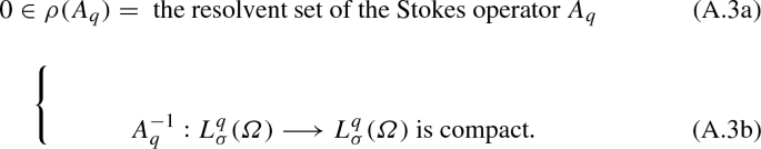
  $$\begin{aligned} \Big ( L^{q}_{\sigma }(\varOmega ),\mathcal {D}(A_q) \Big )_{1-\frac{1}{p},p}&= \Big \{ g \in B^{2-{}^{2}\!/_{p}}_{q,p}(\varOmega ): \text { div } g = 0, \ g|_{\varGamma } = 0 \Big \} \nonumber \\&\text {if } \frac{1}{q}< 2 - \frac{2}{p} < 2; \end{aligned}$$

  (A.8a)
  $$\begin{aligned} \Big ( L^{q}_{\sigma }(\varOmega ),\mathcal {D}(A_q) \Big )_{1-\frac{1}{p},p}&= \Big \{ g \in B^{2-{}^{2}\!/_{p}}_{q,p}(\varOmega ): \text { div } g = 0, \ g\cdot \nu |_{\varGamma } = 0 \Big \} \nonumber \\&\quad \equiv {{\widetilde{B}}}^{2-{}^{2}\!/_{p}}_{q,p}(\varOmega ) \quad \text { if } 0< 2 - \frac{2}{p}< \frac{1}{q}, \text { or } 1< p < \frac{2q}{2q-1}. \end{aligned}$$

  (A.8b)

  In fact, Theorem A.1(i) states that the Stokes operator $-A_q$ generates a s.c analytic semigroup on the space $L^{q}_{\sigma }(\varOmega ), \ 1< q < \infty$, hence on the space ${\mathcal {D}}(A_q)$ in (A.1), with norm $\displaystyle \left\Vert \ \cdot \ \right\Vert _{{\mathcal {D}}(A_q)} = \left\Vert A_q \ \cdot \ \right\Vert _{L^{q}_{\sigma }(\varOmega )}$ as $0 \in \rho (A_q)$. Then, one obtains that the Stokes operator $-A_q$ generates a s.c. analytic semigroup on the real interpolation spaces in (A.8). Next, the Oseen operator ${\mathcal {A}}= -(\nu _o A_q + A_{o,q})$ likewise generates a s.c. analytic semigroup $\displaystyle e^{{\mathcal {A}}_q t}$ on $\displaystyle L^{q}_{\sigma }(\varOmega )$ by Theorem A.1(ii). Moreover ${\mathcal {A}}_q$ generates a s.c. analytic semigroup on $\displaystyle {\mathcal {D}}({\mathcal {A}}_q) = {\mathcal {D}}(A_q)$ (equivalent norms). Hence ${\mathcal {A}}_q$ generates a s.c. analytic semigroup on the real interpolation spaces (A.11). Here below, however, we shall formally state the result only in the case $\displaystyle 2-{}^{2}\!/_{p} < {}^{1}\!/_{q}$. that is $\displaystyle 1< p < {}^{2q}\!/_{2q-1}$, in the space $\displaystyle {{\widetilde{B}}}^{2-{}^{2}\!/_{p}}_{q,p}(\varOmega )$, as this does not contain B.C. The objective of the present paper is precisely to obtain stabilization results on spaces that do not recognize B.C.

Theorem A.3

Let $1< q< \infty , 1< p < {}^{2q}\!/_{2q-1}$

• (i) The Stokes operator $-A_q$ in (A.1) generates a s.c analytic semigroup $e^{-A_qt}$ on the space ${{\widetilde{B}}}^{2-{}^{2}\!/_{p}}_{q,p}(\varOmega )$ defined in (1.15b) which moreover is uniformly stable, as in (A.4),

  $$\begin{aligned} \left\Vert e^{-A_qt}\right\Vert _{{\mathcal {L}}\big ({{\widetilde{B}}}^{2-{}^{2}\!/_{p}}_{q,p}(\varOmega )\big )} \le M e^{-\delta t}, \quad t > 0. \end{aligned}$$

  (A.9)

• (ii) The Oseen operator ${\mathcal {A}}_q$ in (A.2) generates a s.c. analytic semigroup $e^{{\mathcal {A}}_qt}$ on the space ${{\widetilde{B}}}^{2-{}^{2}\!/_{p}}_{q,p}(\varOmega )$ in (1.15b).

• (d) Space of maximal $L^p$ regularity on $L^{q}_{\sigma }(\varOmega )$ of the Stokes operator $-A_q, \ 1< p< \infty , \ 1< q < \infty$ up to $T = \infty$. We shall use the notation of [24] and write $\displaystyle -A_q \in MReg (L^p \big ( 0,\infty ; L^{q}_{\sigma }(\varOmega )\big ))$. We return to the dynamic Stokes problem in $\{\varphi (t,x), \pi (t,x) \}$

  

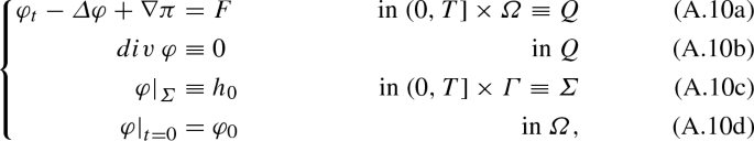
  rewritten in abstract form, after applying the Helmholtz projection $P_q$ to (A.10a) and recalling $A_q$ in (A.1) as

  

  (A.11)

recall (A.8). Next, we introduce the space of maximal regularity for $\{\varphi , \varphi '\}$, that is for $-A_q$, as [39, p 2; Theorem 2.8.5.iii, p 17], [36, p 1404-5], with T up to $\infty$:

$$\begin{aligned} X^T_{p,q, \sigma } (A_q) = L^p(0,T;{\mathcal {D}}(A_q)) \cap W^{1,p}(0,T;L^{q}_{\sigma }(\varOmega )) \end{aligned}$$

(A.12)

(recall (2.14) for ${\mathcal {D}}(A_q)$) and the corresponding space for the pressure as

$$\begin{aligned} Y^T_{p,q} = L^p(0,T;{\widehat{W}}^{1,q}(\varOmega )), \quad {\widehat{W}}^{1,q}(\varOmega ) = W^{1,q}(\varOmega ) / {\mathbb {R}}. \end{aligned}$$

(A.13)

The following embedding, also called trace theorem, holds true [3, Theorem 4.10.2, p 180, BUC for $T=\infty$].

$$\begin{aligned} X^T_{p,q,\sigma }\subset X^T_{p,q}\equiv & {} L^p(0,T; W^{2,q}(\varOmega )) \cap W^{1,p}(0,T; L^q(\varOmega )) \nonumber \\&\hookrightarrow C \Big ([0,T]; B^{2-{}^{2}\!/_{p}}_{q,p}(\varOmega )\Big ). \end{aligned}$$

(A.14)

For a function g such that $div \ g \equiv 0, \ g|_{\varGamma } = 0$ we have $g \in X^T_{p,q}\iff g \in X^T_{p,q,\sigma }$, by (1.4).

The solution of Equation (A.11) is

$$\begin{aligned} \varphi (t) = e^{-A_qt} \varphi _0 + \int _{0}^{t} e^{-A_q(t-\tau )} F_{\sigma }(\tau ) \mathrm{d} \tau . \end{aligned}$$

(A.15)

The following is the celebrated result on maximal regularity on $L^{q}_{\sigma }(\varOmega )$ of the Stokes problem due originally to Solonnikov [70] reported in [39, 64, Theorem 2.8.5(iii) for $\varphi _0 = 0$ and Theorem 2.10.1 p24], [36, 61, Proposition 4.1 , p 1405]. See also [12, Theorem 3.1 p 31 for $p = q =2$ case]. See also [69, 71,72,73].

Theorem A.4

Let $1< p,q < \infty , T \le \infty$. With reference to problem (A.10), (A.11), assume

$$\begin{aligned} F_{\sigma }\in L^p(0,T;L^{q}_{\sigma }(\varOmega )), \ \varphi _0 \in \Big ( L^{q}_{\sigma }(\varOmega ), {\mathcal {D}}(A_q)\Big )_{1-\frac{1}{p},p}. \end{aligned}$$

(A.16)

Then there exists a unique solution $\varphi \in X^T_{p,q,\sigma }$ continuously on the data: there exist constants $C_0, C_1$ independent of $T, F_{\sigma }, \varphi _0$ such that via (A.14)

$$\begin{aligned} \begin{aligned} C_0 \left\Vert \varphi \right\Vert _{C \big ([0,T]; B^{2-{}^{2}\!/_{p}}_{q,p}(\varOmega )\big )}&\le \left\Vert \varphi \right\Vert _{X^T_{p,q,\sigma }} + \left\Vert \pi \right\Vert _{Y^T_{p,q}}\\&= \left\Vert \varphi '\right\Vert _{L^p(0,T;L^{q}_{\sigma }(\varOmega ))} + \left\Vert A_q \varphi \right\Vert _{L^p(0,T;L^{q}_{\sigma }(\varOmega ))} + \left\Vert \pi \right\Vert _{Y^T_{p,q}}\\&\le C_1 \bigg \{ \left\Vert F_{\sigma }\right\Vert _{L^p(0,T;L^{q}_{\sigma }(\varOmega ))} \\&\quad + \left\Vert \varphi _0\right\Vert _{\big ( L^{q}_{\sigma }(\varOmega ), {\mathcal {D}}(A_q)\big )_{1-\frac{1}{p},p}} + \left\Vert h_0\right\Vert _{L^p(0,\infty ; W^{1-{}^{1}\!/_{q},q}(\varGamma ))} \bigg \}.\nonumber \end{aligned}\\ \end{aligned}$$

(A.17)

In particular,

• (i) With reference to the variation of parameters formula (A.15) of problem (A.11) arising from the Stokes problem (A.10), we have recalling (A.12): the map

  $$\begin{aligned} F_{\sigma }&\longrightarrow \int _{0}^{t} e^{-A_q(t-\tau )}F_{\sigma }(\tau ) \mathrm{d}\tau : \ : \text {continuous} \end{aligned}$$

  (A.18)
  $$\begin{aligned} L^p(0,T;L^{q}_{\sigma }(\varOmega ))&\longrightarrow X^T_{p,q,\sigma }(A_q) \equiv L^p(0,T; {\mathcal {D}}(A_q)) \cap W^{1,p}(0,T; L^{q}_{\sigma }(\varOmega )). \end{aligned}$$

  (A.19)

• (ii) The s.c. analytic semigroup $e^{-A_q t}$ generated by the Stokes operator $-A_q$ (see (A.1)) on the space $\displaystyle \Big ( L^{q}_{\sigma }(\varOmega ), {\mathcal {D}}(A_q)\Big )_{1-\frac{1}{p},p}$ satisfies

  $$\begin{aligned}&e^{-A_q t}: \ \text {continuous} \quad \Big ( L^{q}_{\sigma }(\varOmega ), {\mathcal {D}}(A_q)\Big )_{1-\frac{1}{p},p} \longrightarrow \nonumber \\&\quad X^T_{p,q,\sigma }(A_q) \equiv L^p(0,T; {\mathcal {D}}(A_q)) \cap W^{1,p}(0,T; L^{q}_{\sigma }(\varOmega )). \end{aligned}$$

  (A.20a)

  In particular via (A.8b), for future use, for $1< q< \infty , 1< p < \frac{2q}{2q - 1}$, the s.c. analytic semigroup $\displaystyle e^{-A_q t}$ on the space $\displaystyle {{\widetilde{B}}}^{2-{}^{2}\!/_{p}}_{q,p}(\varOmega )$, satisfies

  $$\begin{aligned} e^{-A_q t}: \ \text {continuous} \quad {{\widetilde{B}}}^{2-{}^{2}\!/_{p}}_{q,p}(\varOmega )\longrightarrow X^T_{p,q,\sigma }. \end{aligned}$$

  (A.20b)

• (iii) Moreover, setting $\nabla \pi = (Id - P_q)(\varDelta + F)$, it follows that $\{ \varphi , \pi \} \in X^T_{p,q,\sigma }\times Y^T_{p,q}$, see (A.13), solves problem (A.10) and there is a constant $C>0$ independent of $T,F_{\sigma },\phi _0$ s.t.

  $$\begin{aligned} \left\Vert \varphi \right\Vert _{X^T_{p,q,\sigma }} + \left\Vert \pi \right\Vert _{Y^T_{p,q}} \le C \bigg \{ \left\Vert F_{\sigma }\right\Vert _{L^p(0,T;L^{q}_{\sigma }(\varOmega ))} + \left\Vert \varphi _0\right\Vert _{\big ( L^{q}_{\sigma }(\varOmega ), {\mathcal {D}}(A_q) \big )_{1-\frac{1}{p},p}} \bigg \}\nonumber \\ \end{aligned}$$

  (A.21a)

  while, for future use, for $1< q< \infty , 1< p < \frac{2q}{2q - 1}$, then (A.21a) specializes to

  $$\begin{aligned} \left\Vert \varphi \right\Vert _{X^T_{p,q,\sigma }} + \left\Vert \pi \right\Vert _{Y^T_{p,q}} \le C \bigg \{ \left\Vert F_{\sigma }\right\Vert _{L^p(0,T;L^{q}_{\sigma }(\varOmega ))} + \left\Vert \varphi _0\right\Vert _{{{\widetilde{B}}}^{2-{}^{2}\!/_{p}}_{q,p}(\varOmega )} \bigg \}.\nonumber \\ \end{aligned}$$

  (A.21b)

• (e) Maximal $L^p$ regularity on $L^{q}_{\sigma }(\varOmega )$ of the Oseen operator $\displaystyle {\mathcal {A}}_q, \ 1< p< \infty , \ 1< q < \infty$: $\displaystyle {\mathcal {A}}_q \in MReg (L^p(0,T;L^{q}_{\sigma }(\varOmega )))$, T finite arbitrary. We next transfer the maximal regularity of the Stokes operator $(-A_q)$ on $L^{q}_{\sigma }(\varOmega )$-asserted in Theorem A.4 into the maximal regularity of the Oseen operator ${\mathcal {A}}_q = -\nu _o A_q - A_{o,q}$ exactly on the same space $X^T_{p,q,\sigma }$ defined in (A.12), except now only on $T < \infty$.

Thus, consider the dynamic Oseen problem in $\{ \psi (t,x), \pi (t,x) \}$ with equilibrium solution $y_e$, see Theorem 1.1 on (1.2) :

(A.23)

rewritten in abstract form, after applying the Helmholtz projector $P_q$ to (A.22a) and recalling ${\mathcal {A}}_q$ in (A.2)

$$\begin{aligned} \psi _t = {\mathcal {A}}_q \psi + P_q F = -\nu _o A_q \psi - A_{o,q} \psi + F_{\sigma }, \quad \psi _0 \in \big ( L^{q}_{\sigma }(\varOmega ), {\mathcal {D}}(A_q)\big )_{1-\frac{1}{p},p}\nonumber \\ \end{aligned}$$

(A.24)

whose solution is

$$\begin{aligned} \psi (t)= & {} e^{{\mathcal {A}}_qt} \psi _0 + \int _{0}^{t} e^{{\mathcal {A}}_q(t-\tau )} Fs(\tau ) \mathrm{d} \tau . \end{aligned}$$

(A.25)

$$\begin{aligned} \psi (t)= & {} e^{- \nu _o A_qt} \psi _0 + \int _{0}^{t} e^{-\nu _o A_q(t-\tau )} F_{\sigma }(\tau ) \mathrm{d} \tau - \int _{0}^{t} e^{- \nu _o A_q(t-\tau )} A_{o,q} \psi (\tau ) \mathrm{d} \tau .\nonumber \\ \end{aligned}$$

(A.26)

Theorem A.5

Let $1< p,q < \infty$, $0< T < \infty$. Assume (as in (A.16))

$$\begin{aligned} F_{\sigma }\in L^p \big ( 0, T; L^q_{\sigma } (\varOmega ) \big ), \quad \psi _0 \in \big ( L^{q}_{\sigma }(\varOmega ), {\mathcal {D}}(A_q) \big )_{1-\frac{1}{p},p}\end{aligned}$$

(A.27)

where ${\mathcal {D}}(A_q) = {\mathcal {D}}({\mathcal {A}}_q)$, see (A.2). Then there exists a unique solution $\psi \in X^T_{p,q,\sigma }$ of the dynamic Oseen problem (A.22), continuously on the data: that is, there exist constants $C_{0T}, C_{1T}$ independent of $F_{\sigma }, \psi _0$ such that (recall (A.14)):

$$\begin{aligned} C_{0T} \left\Vert \psi \right\Vert _{C \big ([0,T]; B^{2-{}^{2}\!/_{p}}_{q,p}(\varOmega )\big )}&\le \left\Vert \psi \right\Vert _{X^T_{p,q,\sigma }} + \left\Vert \pi \right\Vert _{Y^T_{p,q}} \nonumber \\&\equiv \left\Vert \psi '\right\Vert _{L^p(0,T;L^q(\varOmega ))} + \left\Vert A_q \psi \right\Vert _{L^p(0,T;L^q(\varOmega ))} + \left\Vert \pi \right\Vert _{Y^T_{p,q}} \end{aligned}$$

(A.28)

$$\begin{aligned}&\le C_{1T} \bigg \{ \left\Vert F_{\sigma }\right\Vert _{L^p(0,T;L^{q}_{\sigma }(\varOmega ))} + \left\Vert \psi _0\right\Vert _{\big ( L^{q}_{\sigma }(\varOmega ), {\mathcal {D}}(A_q) \big )_{1-\frac{1}{p},p}} \bigg \} \end{aligned}$$

(A.29)

Equivalently, for $1< p, q < \infty$

• i. The map

  $$\begin{aligned} \begin{aligned} F_{\sigma }\longrightarrow \int _{0}^{t} e^{{\mathcal {A}}_q(t-\tau )}F_{\sigma }(\tau ) \mathrm{d}\tau : \ : \text {continuous}&\\ L^p(0,T;L^{q}_{\sigma }(\varOmega ))&\longrightarrow L^p \big (0,T;{\mathcal {D}}({\mathcal {A}}_q) = {\mathcal {D}}(A_q) \big )\nonumber \end{aligned}\\ \end{aligned}$$

  (A.30)

  where then automatically, see (A.24)

  $$\begin{aligned} L^p(0,T;L^{q}_{\sigma }(\varOmega )) \longrightarrow W^{1,p}(0,T;L^{q}_{\sigma }(\varOmega )) \end{aligned}$$

  (A.31)

  and ultimately

  $$\begin{aligned} L^p(0,T;L^{q}_{\sigma }(\varOmega ))\! \longrightarrow \!X^T_{p,q,\sigma }(A_q) \!\equiv \! L^p \big (0,T;{\mathcal {D}}(A_q) \big ) \!\cap \! W^{1,p}(0,T;L^{q}_{\sigma }(\varOmega )).\nonumber \\ \end{aligned}$$

  (A.32a)

  Thus,

  $$\begin{aligned} {\mathcal {A}}_q \in MReg (L^p(0,T;L^{q}_{\sigma }(\varOmega ))), \ 1< T < \infty \end{aligned}$$

  (A.32b)

  and the operator $\displaystyle {\mathcal {A}}_q$ has maximal $L^p$ regularity on $L^{q}_{\sigma }(\varOmega )$.

• ii. The s.c. analytic semigroup $e^{{\mathcal {A}}_q t}$ generated by the Oseen operator ${\mathcal {A}}_q$ (see (A.2)) on the space $\displaystyle \big ( L^{q}_{\sigma }(\varOmega ), {\mathcal {D}}(A_q) \big )_{1-\frac{1}{p},p}$ satisfies for $1< p, q < \infty$

  $$\begin{aligned} e^{{\mathcal {A}}_q t}: \ \text {continuous} \quad \big ( L^{q}_{\sigma }(\varOmega ), {\mathcal {D}}(A_q) \big )_{1-\frac{1}{p},p}\longrightarrow L^p \big (0,T;{\mathcal {D}}({\mathcal {A}}_q) = {\mathcal {D}}(A_q) \big ) \nonumber \\ \end{aligned}$$

  (A.33)

  and hence automatically

  $$\begin{aligned} e^{ {\mathcal {A}}_q t}: \ \text {continuous} \quad \big ( L^{q}_{\sigma }(\varOmega ), {\mathcal {D}}(A_q) \big )_{1-\frac{1}{p},p}\longrightarrow X^T_{p,q,\sigma }. \end{aligned}$$

  (A.34)

  In particular, for future use, for $1< q< \infty , 1< p < \frac{2q}{2q - 1}$, we have that the s.c. analytic semigroup $\displaystyle e^{{\mathcal {A}}_q t}$ on the space $\displaystyle {{\widetilde{B}}}^{2-{}^{2}\!/_{p}}_{q,p}(\varOmega )$, satisfies

  $$\begin{aligned} e^{{\mathcal {A}}_q t}: \ \text {continuous} \quad {{\widetilde{B}}}^{2-{}^{2}\!/_{p}}_{q,p}(\varOmega )\longrightarrow L^p \big (0,T;{\mathcal {D}}({\mathcal {A}}_q) = {\mathcal {D}}(A_q) \big ), \ T < \infty , \nonumber \\ \end{aligned}$$

  (A.35)

  and hence automatically

  $$\begin{aligned} e^{ {\mathcal {A}}_q t}: \ \text {continuous} \quad {{\widetilde{B}}}^{2-{}^{2}\!/_{p}}_{q,p}(\varOmega )\longrightarrow X^T_{p,q,\sigma }(A_q), \ T < \infty . \end{aligned}$$

  (A.36)

• iii. An estimate such as the one in (A.21a) applies to the pressure $\pi$, where now $\displaystyle \nabla \pi (Id - P_q)(\varDelta - L_e + F)$.

A proof of Theorem A.5 is given in [50].

Appendix B: The Eigenvectors $\displaystyle \varphi ^*_{ij} \in W^{2,q'}(\varOmega ) \cap W^{1,q'}_0(\varOmega ) \cap L^{q'}_{\sigma }(\varOmega )$ of $\displaystyle {\mathcal {A}}^* (={\mathcal {A}}_q^*)$ in $\displaystyle L^{q'}(\varOmega )$ May Be Viewed Also as $\displaystyle \varphi ^*_{ij} \in W^{3,q}(\varOmega )$, so that $\displaystyle \frac{\partial \varphi ^*_{ij}}{\partial \nu } \bigg |_{\varGamma } \in W^{2-{}^{1}\!/_{q},q}(\varGamma ), \ q \ge 2$.

The eigenvectors $\displaystyle \varphi ^*_{ij}$ of $\displaystyle {\mathcal {A}}^* (={\mathcal {A}}_q^*)$, defined in (4.8a), are in $\displaystyle {\mathcal {D}}(({\mathcal {A}}_q^*)^n)$ for any n, so the are arbitrarily smooth in $L^{q'}_{\sigma }(\varOmega )$, say $\displaystyle \varphi ^*_{ij} \in W^{s,q'}(\varOmega )$, with s as large as we please. We seek to view $\displaystyle \varphi ^*_{ij}$ in an $\displaystyle L^q(\varOmega )$-based space. To this end, we recall a Sobolev embedding theorem.

Theorem B.1

[81, p328], For a more restricted version [1, p 97] Let $\varOmega$ be an arbitrary bounded domain, dim $\varOmega = d$. Let $0 \le t \le s < \infty$ and $\infty> q \ge {\widetilde{q}} > 1$. Then, the following embedding holds true:

$$\begin{aligned} W^{s,{\widetilde{q}}}(\varOmega ) \subset W^{t, q}(\varOmega ), \ s - \frac{d}{{\widetilde{q}}} \ge t - \frac{d}{q} \quad \end{aligned}$$

(B.1)

$\square$

Corollary B.2

With $\displaystyle 2 \le q < \infty , \ {}^{1}\!/_{q} + {}^{1}\!/_{q'} = 1$, so that $\displaystyle 1 < q' \le 2 \le q, \ 0 \le r$, we have

• (i)
  $$\begin{aligned} \varphi ^*_{ij} \in W^{r+m, q'}(\varOmega ) \subset W^{r,q}(\varOmega ), \quad m \ge d \left( \frac{1}{q} + \frac{1}{q'} \right) = \left\{ \begin{array}{ll} 0, &{} q' = q = 2 \\ d, &{} q' = 1, q = \infty \end{array}\right. \nonumber \\ \end{aligned}$$

  (B.2)
• (ii)
  $$\begin{aligned} \frac{\partial \varphi ^*_{ij}}{\partial \nu } \bigg |_{\varGamma } \in W^{r-1-{}^{1}\!/_{q},q}(\varGamma ), \quad r > 1 + \frac{1}{q} \quad \end{aligned}$$

  (B.3)

• (iii) With reference to the sub-space ${\mathcal {F}}$ based on $\varGamma$, as defined in (1.25), we have

  $$\begin{aligned} {\mathcal {F}}\equiv & {} \text{ span }\left\{ \frac{\partial }{\partial \nu } \varphi ^*_{ij}, \ i = 1,\ldots ,M; \ j = 1,\ldots ,\ell _i\right\} \nonumber \\\subset & {} W^{r-1-{}^{1}\!/_{q},q}(\varGamma ), \ r > 1 + \frac{1}{q} \end{aligned}$$

  (B.4)

  In particular, for our purposes, if will suffice to take $r=3$ in (B.2), so that (B.2)–(B.4) become

  $$\begin{aligned} \varphi ^*_{ij} \in W^{3,q}(\varOmega ), \quad \frac{\partial \varphi ^*_{ij}}{\partial \nu } \bigg |_{\varGamma } \in W^{2-{}^{1}\!/_{q},q}(\varGamma ), \quad {\mathcal {F}}\subset W^{2-{}^{1}\!/_{q},q}(\varGamma ). \end{aligned}$$

  (B.5)

• (iv) Thus, with reference to the boundary vector $v = v_N$ introduced in (5.1) = (6.10), we have

  $$\begin{aligned} v = \sum _{k=1}^{K} \nu _k(t) f_k \in W^{2-{}^{1}\!/_{q},q}(\varGamma ), \ f_k \in {\mathcal {F}}, \ f_k \cdot \nu |_{\varGamma } = 0, \ v \cdot \nu |_{\varGamma } = 0 \nonumber \\ \end{aligned}$$

  (B.6)

• (v) Recalling the Dirichlet map D introduced to describe the solution of problem (2.1), we have

  $$\begin{aligned} Dv \in W^{2,q}(\varOmega ), \quad 2 \le q < \infty \end{aligned}$$

  (B.7)

Proof

(i) Apply Theorem B.1 with $\displaystyle s = r + m \ge t = r, \ {\widetilde{q}} = q', \ {}^{1}\!/_{q} + {}^{1}\!/_{q'} = 1, \ q \ge 2$, so that $\displaystyle q' = {\widetilde{q}} \le q$, to verify that the required condition (B.1)

$$\begin{aligned} s - \frac{d}{{\widetilde{q}}} = r + m - \frac{d}{q'} \ge t - \frac{d}{q} = r - \frac{d}{q}, \ \text {or} \ m \ge d \left( \frac{1}{q'} - \frac{1}{q} \right) \ge 0 \end{aligned}$$

(B.8)

can always be satisfied by taking $m \ge 0$ suitable as in (B.8). This is possible, since $\displaystyle \varphi ^*_{ij}$ is arbitrarily smooth.

(ii) Then (B.3) follows by the usual trace theory [1].

Then, (iii)–(v) readily follow, as D improves regularity by ${}^{1}\!/_{q}$ from the boundary to the interior. $\square$

Next, we return to the operator $\displaystyle F: L^q(\varOmega ) \subset L^{q}_{\sigma }(\varOmega )\longrightarrow L^q(\varGamma )$ in (5.6). Its adjoint $F^*$ is

$$\begin{aligned} F^*g = \sum _{k = 1}^{K} (f_k, g)_{_{\varGamma }} p_k \in (W^u_N)^* \subset L^{q'}_{\sigma }(\varOmega ), \quad g \in L^q(\varGamma ) \end{aligned}$$

(B.9)

where we have seen in (2.64) that $\displaystyle D: L^q(\varGamma ) \supset U_q \longrightarrow W^{{}^{1}\!/_{q},q}(\varOmega ) \cap L^{q}_{\sigma }(\varOmega )\subset {\mathcal {D}}\Big ( A^{{}^{1}\!/_{2q} - \varepsilon }_q \Big )$

$$\begin{aligned} F^*D^*h = \sum _{k = 1}^{K} (f_k, D^*h)_{_{\varGamma }} p_k = \sum _{k = 1}^{K} \big < Df_k, h \big >_{_{W^u_N}} p_k \in (W^u_N)^* \end{aligned}$$

(B.10)

where we have conservatively: $\displaystyle f_k \in L^{q'}(\varGamma ), \ f_k \cdot \nu = 0$ on $\varGamma$, thus by (2.9), $\displaystyle Df_k \in W^{{}^{1}\!/_{q'},q'}(\varOmega ) = W^{{}^{1}\!/_{q'},q'}_0(\varOmega )$ by (2.63a) since $\displaystyle {}^{1}\!/_{q'} \le q'$ for $1 < q' \le 2$. Thus, in (B.10) we can take $\displaystyle h \in W^{-{}^{1}\!/_{q},q}(\varOmega )$. In particular

$$\begin{aligned} F^*D^* \in {\mathcal {L}}\big (L^{q'}(\varOmega )\big ), \quad 1 < q' \le 2. \end{aligned}$$

(B.11)

Appendix C: Relevant Unique Continuation Properties for Overdetermined Oseen Eigenvalue Problems

In this Appendix C, we assemble a comprehensive account of unique continuation problems for Oseen eigenproblems, as they pertain to the problem of controllability of finite dimensional projected system (4.8a, 4.8b) of the linearized w-problem (1.28) (with interior, tangential-like localized control $u \equiv 0$). Positive solution, or lack thereof, of this finite dimensional problem is a key step, or obstruction, for the uniform stabilization of the Navier Stokes equations. This issue has been known since the study of boundary feedback stabilization of a parabolic equation with Dirichlet boundary trace in the feedback loop, as acting on the Neumann boundary conditions [54]. We return to the bounded domain $\varOmega , \ d = 2,3,$ with boundary $\varGamma = \partial \varOmega$. As before, ${\widetilde{\varGamma }}$ is a subportion of $\varGamma$.

Problem #1 (over-determination only on a portion ${\widetilde{\varGamma }}$ of $\varGamma$) Let $\{\varphi , p\} \in W^{2,q}(\varOmega ) \times W^{1,q}(\varOmega )$ solve the over-determined problem

with over-determination only on the portion ${\widetilde{\varGamma }}$ of $\varGamma$. Does (C.1a, C.1b, C.1c) imply

(C.2)

The answer is negative even in the Stokes case: $L_e(\varphi ) \equiv 0$. This follows from [26], where the following counterexample is given in the 2-dimensional half-space $\varOmega = \{(x,y) : x \in {\mathbb {R}}^+, y \in {\mathbb {R}}\}$ with boundary $\varGamma = \{ x = 0 \}$. On $\varOmega$ take

$$\begin{aligned} u_1(x,y) \equiv 0, \quad u_2(x,y) = ax^2, \quad p = 2ay, \quad a \ne 0, \end{aligned}$$

(C.3)

so that with $u = \{u_1, u_2\}$, it follows that

$$\begin{aligned} \varDelta u = \nabla p \text { in } \varOmega , \quad u|_{\varGamma } = \nabla u|_{\varGamma } = 0, \end{aligned}$$

(C.4)

to obtain a nontrivial solution of the Stokes overdetermined eigenproblem with $\lambda = 0$. Such half-space example can then be transformed into a counterexample over the bounded domain $\varOmega$ where the over-determination is active on any subset ${\widetilde{\varGamma }}$ of the boundary $\varGamma = \partial \varOmega$.

Implications of failure of unique continuation under Problem #1: A negative consequence of the lack of unique continuation (C.1) $\implies$ (C.2) with over-determination only in a portion ${\widetilde{\varGamma }}$ of the boundary $\varGamma$ is as follows: that global uniform stabilization of the linearized w-problem (1.28) by means of a purely tangential (finite or infinite dimensional) feedback boundary control v (as given by (5.1) in the finite dimensional case) acting only on a small subportion ${\widetilde{\varGamma }}$ of the boundary $\varGamma$ (and thus with localized interior tangential-like control $u \equiv 0$) is not possible. This is so since the algebraic rank condition (4.11b) (with $u \equiv 0$) fails, as boundary traces

$$\begin{aligned} \left\{ \left. \frac{\partial \varphi ^*_{i1}}{\partial \nu }\right| _{{\widetilde{\varGamma }}}, \left. \frac{\partial \varphi ^*_{i2}}{\partial \nu }\right| _{{\widetilde{\varGamma }}}, \dots , \left. \frac{\partial \varphi ^*_{i \ell _i}}{\partial \nu }\right| _{{\widetilde{\varGamma }}} \right\} \text { fail to be linearly independent on } {\widetilde{\varGamma }} \end{aligned}$$

(C.5)

since, equivalently, the implication (C.1)$\implies$(C.2) fails. See Orientation.

Problem #2 (dual of the statement of Lemma 4.3): necessity to complement the localized control v on ${\widetilde{\varGamma }}$ with a localized interior tangential-like control u supported on $\omega$ in terms of ${\widetilde{\varGamma }}$. Let now $\{ \varphi , p \} \in W^{2,q}(\varOmega ) \times W^{1,q}(\varOmega )$ solve the problem

Then, [53, Theorem 6.2],

$$\begin{aligned} \varphi \equiv 0 \quad \text {and} \quad p \equiv \text {const} \quad \text {in } \varOmega . \end{aligned}$$

(C.7)

It is as a consequence of such unique continuation property that the Kalman algebraic rank conditions (6.28b) are satisfied. This is the basic result upon which the uniform stabilization of the present paper relies. Thus we can conclude that the results of the present paper (as in [53]) are optimal in terms of the required extra condition of the localized interior, tangential-like control needed to supplement the insufficient role of the localized tangential boundary control v on ${\widetilde{\varGamma }}$. Optimality is in terms of the smallness of the required control action for v and u.

Problem #3 (over-determination on the entire boundary $\varGamma = \partial \varOmega$). Let now $\{ \varphi , p \} \in W^{2,q}(\varOmega ) \times W^{1,q}(\varOmega )$ solve the over-determined problem

with over-determination on all of $\varGamma$. Then, does (C.8a, C.8b, C.8c) imply

(C.9)

It seems that a general definitive answer is not known at present. Only partial results are known.

The desired unique continuation (C.8)$\implies$(C.9) holds true, if the equilibrium solution $y_e \equiv 0$ (Stokes eigenproblem) or, more generally, if $y_e$ is sufficiently small in the $W^{1,q}(\varOmega )$-norm. Several different proofs are given in [79, 80].

The case $y_e \equiv 0$ is actually physically quite important as it occurs for instance when the forcing function in (1.1a) or (1.2a) is a conservative vector field (say an electrostatic or gravitational field) $f = \nabla g$. In this case, a solution (1.2a, 1.2b, 1.2c) is: $\displaystyle y_e \equiv 0, \ \pi _e = g$.

When $y_e \equiv 0$ (or $y_e$ small) the tangential boundary feedback control v alone, in the form such as (5.1), as acting on the entire boundary $\varGamma$ produces enhancement of stability at will for the linearized w-problem.

Of course, with $y_e \equiv 0$, the corresponding Oseen problems reduces to the Stokes problem. The Stokes semigroup is already uniformly stable, see (3.7), with margin of stability $\delta > 0$. When $y_e \equiv 0$ a most valuable variation of the problem under investigation of the present paper is to enhance the original margin of stability $\delta > 0$ of the original linearized uncontrolled w-problem (1.11) (with $u \equiv 0, \ v \equiv 0$) to obtain an arbitrary decay rate, say $k^2$, by means of only a tangential boundary finite dimensional feedback control, of the same form as the operator F in (5.6b) but applied to all of $\varGamma$. To this, it suffices to apply the procedure of the present paper to a finite dimensional projected space spanned by the eigenvectors of the Stokes operator corresponding to finitely many eigenvalues $\lambda _i, \ i = 1, \dots , I$,

$$\begin{aligned} -k^2 \le - Re \ \lambda _I \le \dots \le Re \ \lambda _1 \le -\delta \end{aligned}$$

(C.10)

Problem #4 over-determination on a portion of the boundary ${\widetilde{\varGamma }}$ involving also the pressure p. Let $\{\varphi , p\} \in W^{2,q}(\varOmega ) \cap W^{1,q}(\varOmega )$ solve the over-determined problem

Does this imply

(C.12)

This answer is in the affirmative. The argument, given in the [79] is along more classical elliptic arguments [45]. Here however the new condition in (C.11c) contains the pressure, which must be viewed as unknown in general. Application of this result to the present paper will result in substituting $\displaystyle \partial _{\nu } \varphi _{ij}^*|_{{\widetilde{\varGamma }}}$ with $\displaystyle [\partial _{\nu } \varphi _{ij}^* - p_i \nu ]|_{{\widetilde{\varGamma }}}$ in the matrix $W_i$ in (4.9), which then—with this modification—becomes full rank, as desired. Thus, the stabilizing control will be expressed in terms of the pressure on the boundary, which is typically unknown.

References

Adams, R.A.: Sobolev Spaces. Academic Press, London, 1975
Amann, H.: Linear and Quasilinear Parabolic Problems. Birkhäuser, London, 1995
Amann, H.: On the strong solvability of the Navier–Stokes equations. J. Math. Fluid Mech. 2, 16–98, 2000
Amrouche, C., Rodriguez-Bellido, M.A.: Stationary Stokes, Oseen and Navier–Stokes Equations with Singular Data. hal-00549166, 2010
Badra, M., Takahashi, T.: Stabilization of parabolic nonlinear systems with finite dimensional feedback or dynamical controllers: application to the Navier–Stokes system. SIAM J. Control Optim. 49(2), 420–463. https://doi.org/10.1137/090778146
Balakrishnan, A.V.: Applied Functional Analysis, Applications of Mathematics Series, 2nd edn. Springer, 369, 1981
Balogh, A., Liu, W.J., Krstic, M.: Stability enhancement by boundary control in 2D channel flow. IEEE Trans. Autom. Control 46, 1696–1711, 2001
Barbu, V.: Stabilization of Navier–Stokes Flows. Springer, 276, 2011
Barbu, V.: Controllability and Stabilization of Parabolic Equations. Birkhäuser, Bessel, 226, 2018
Barbu, V., Lasiecka, I.: The unique continuation property of eigenfunctions to Stokes–Oseen operator is generic with respect to the coefficients. Nonlinear Anal. Theory Methods Appl. 75, 4384–4397, 2012
Barbu, V., Triggiani, R.: Internal stabilization of Navier–Stokes equations with finite-dimensional controllers. Indiana Univ. Math. 123, 1443–1494, 2004
Barbu, V., Lasiecka, I., Triggiani, R.: Tangential Boundary Stabilization of Navier–Stokes Equations. Memoires of American Math Society, London, 2006
Barbu, V., Lasiecka, I., Triggiani, R.: Abstract settings for tangential boundary stabilization of Navier–Stokes equations by high- and low-gain feedback controllers. Nonlinear Anal., 64, 2704–2746, 2006
Barbu, V., Lasiecka, I., Triggiani, R.: Local exponential stabilization strategies of the Navier–Stokes equations, d = 2,3 via feedback stabilization of its linearization. Control of Coupled Partial Differential Equations, ISNM, vol. 155, 13–46. Birkhauser, 2007
Borggard, J.: Talk Presented at the Seminar in Control Theory at the IMA. University of Minnesota, 2016
Bradshaw, Z., Grujic, Z.: Frequency localized regularity criteria for the 3D Navier Stokes equations. ARNA 224, 125–133, 2017.
Cannarsa, P., Vespri, V.: On maximal \(L^p\) regularity for the abstract Cauchy problem. Boll. Un. Mat. Ital B (6) 5(1), 165–175, 1986
Chowdhury, S., Mitra, D., Renardy, M.: Null controllability of the incompressible Stokes equations in a 2-D channel using normal boundary control. Evol. Equ. Control Theory 7(3), 447–463, 2018
Constantin, P., Foias, C.: Navier–Stokes Equations (Chicago Lectures in Mathematics), 1st edn, 1980
Danchin, R., Mucha, P.B.: New maximal regularity results for the heat equation in exterior domains, and applications. Studies in Phase Space Analysis with Applications to PDEs, Progress in Nonlinear Differential Equations and their applications, vol. 84. Birkhäuser, 2013
Danchin, R., Mucha, P.B.: Critical functional framework and maximal regularity in action on systems of incompressible flows. Memoires 143, 151, 2015
DaPrato, G., Vespri, V.: Maximal \(L^p\) regularity for elliptic equations with unbounded coefficients. Nonlinear Anal. Ser. A Theory Methods 49(6), 747–755, 2002
Dascaliuc, R., Grujić, Z.: On energy cascades in the forced 3D Navier–Stokes equations. J. Nonlinear Sci. 26(3), 683–715, 2016
Dore, G.: Maximal regularity in \(L^p\) spaces for an abstract Cauchy problem. Adv. Differ. Equ., 2000
Escauriaza, L., Seregin, G., Šverák, V.: \(L_{3,\infty }\)-solutions of Navier–Stokes equations and backward uniqueness. Math. Subj. Classif. 35K, 76D, 1991
Fabre, C., Lebeau, G.: Prolongement unique des solutions de l’équation de Stokes. Commun. Partial Differ. Equ. 21, 573–596, 1996
Fabes, E., Mendez, O., Mitrea, M.: Boundary. J. Funct. Anal. 159(2), 323–368, 1998
Fattorini, H.O.: The Cauchy Problem Encyclopedia of Mathematics and its Applications (18). Cambridge University Press, 1984. ISBN 9780511662799
Fursikov, A.: Real processes corresponding to the 3D Navier–Stokes system, and its feedback stabilization from the boundary. Partial Differential Equations, American Mathematical Society Translations: Series 2, vol. 260. AMS, Providence, RI, 2002
Fursikov, A.: Stabilizability of two dimensional Navier–Stokes equations with help of a boundary feedback control. J. Math. Fluid Mech. 3, 259–301, 2001
Fursikov, A.: Stabilization for the 3D Navier–Stokes system by feedback boundary control. DCDS 10, 289–314, 2004
Fursikov, A., Gorshkov, A.: Certain questions of feedback stabilization for Navier–Stokes equations. Evol. Equ. Control Theory 109–140, 2012
Foias, C., Temam, R.: Determination of the solution of the Navier–Stokes equations by a set of nodal volumes. Math. Comput. 43(167), 117–133, 1984
Galdi, G.P.: An Introduction to the Mathematical Theory of the Navier–Stokes Equations. Springer, New York, 2011
Gallagher, I., Koch, G.S., Planchon, F.: A profile decomposition approach to the \(L^{\infty }_t (L^3_x)\) Navier–Stokes regularity criterion. Math. Ann. 355(4), 1527–1559, 2013
Geissert, M., Götze, K., Hieber, M.: \({L}_p\)-theory for strong solutions to fluid-rigid body interaction in Newtonian and generalized Newtonian fluids. Trans. Am. Math. Soc., 2013
Giga, Y.: Analyticity of the semigroup generated by the Stokes operator in \(L_r\) spaces. Math. Z. 178(3), 279–329, 1981
Giga, Y.: Domains of fractional powers of the Stokes operator in \(L_r\) spaces. Arch. Ration. Mech. Anal. 89(3), 251–265, 1985
Hieber, M., Saal, J.: The Stokes Equation in the\(L^p\)-Setting: Well Posedness and Regularity Properties Handbook of Mathematical Analysis in Mechanics of Viscous Fluids. Springer, Cham, 2016
Hytónen, T., van Neerven, J., Veraar, M., Weis, L.: Analysis in Banach Spaces, vols. 1 & 2. Springer, 2016.
Jia, H., Šverák, V.: Minimal \(L^3\)-initial data for potential Navier–Stokes singularities. SIAM J. Math. Anal. 45(3), 1448–1459, 2013
Kato, T.: Perturbation Theory of Linear Operators. Springer, Berlin, 1966
Keefe, L.R.: Method and Apparatus for Reducing the Drag of Flows Over Surfaces. US Patent - US 5803409, 1998
Kesavan, S.: Topics in Functional Analysis and Applications. New Age International Publisher, London, 1989
Komornik, V.: Exact Controllability and Stabilization, The Multiplier Theory. Wiley-Masson Series Research in Applied Mathematics, 166, 1996
Kukavica, I., Tuffaha, A.: Regularity solutions to a free boundary problem of fluid-structure interaction. Indiana Univ. Math. J. 61(5), 1817–1859, 2012
Kunstmann, P.C., Weis, L.: Perturbation theorems for maximal \(L^p\)-regularity Annali della Scuola Normale Superiore di Pisa - Classe di Scienze, Série 4 30(2), 415–435, 2001
Kunstmann, P.C., Weis, L.: Maximal \(L^p\)-regularity for parabolic equations, fourier multiplier theorems and \(H^{\infty }\)-functional calculus. Functional Analytic Methods for Evolution Equations, Lecture Notes in Mathematics, vol. 1855, 65–311. Springer, Berlin, 2004
Ladyzhenskaya, O.A.: The Mathematical Theory of Viscous Incompressible Flow, Gordon and Breach, New York English transl., \(2^{\text{nd}}\) edn, 1969
Lasiecka, I., Priyasad, B., Triggiani, R.: Uniform stabilization of Navier–Stokes equations in critical \(L^q\)-based Sobolev and Besov spaces by finite dimensional interior localized feedback controls. Appl. Math. Optim., 2019. https://doi.org/10.1007/s00245-019-09607-9
Lasiecka, I., Triggiani, R.: Control theory for partial differential equations: continuous and approximation theories, vol. 1, abstract parabolic systems (680 pp.). Encyclopedia of Mathematics and its Applications Series, Cambridge University Press, 2000
Lasiecka, I., Triggiani, R.: Uniform stabilization with arbitrary decay rates of the Oseen equation by finite-dimensional tangential localized interior and boundary controls. Semigroups Oper. Theory Appl. 113, 125–154, 2015
Lasiecka, I., Triggiani, R.: Stabilization to an equilibrium of the Navier–Stokes equations with tangential action of feedback controllers. Nonlinear Anal. 121, 424–446, 2015.
Lasiecka, I., Triggiani, R.: Stabilization of Neumann boundary feedback of parabolic equations: the case of trace in the feedback loop. Appl. Math. Optim. 10(1), 307–350, 1983
Leray, J.: Sur le mouvement d’un liquide visquex emplissent l’espace. Acta Math. J. 63, 193–248, 1934
Lions, J.L.: Quelques Methodes de Resolutions des Problemes aux Limites Non Lineaire. Dunod, Paris, 1969
Lions, J.L., Magenes, E.: Non-homogeneous Boundary Value Problems and Applications, Springer, London, 1972
Maslenniskova, V., Bogovskii, M.: Elliptic boundary values in unbounded domains with non compact and non smooth boundaries. Rend. Sem. Mat. Fis. Milano, 56, 125–138, 1986
Mazya, V.G., Shaposhnikova, T.O.: Theory of multipliers in spaces of differentiable functions. Monogr. Stud. Math. 23, 1985. https://doi.org/10.1016/B978-0-08-026491-2.50010-9
Pazy, A.: Semigroups of Linear Operators and Applications to Partial Differential Equations. Springer, 1983
Prüss, J., Simonett, G.: Moving Interfaces and Quasilinear Parabolic Evolution Equations. Monographs in Mathematics, vol. 105. Birkhüuser, Basel, 2016
Raymond, J.-P.: Feedback boundary stabilization of the three-dimensional incompressible Navier–Stokes equations. Journal de Mathématiques Pures et Appliquées 87(6), 627–669, 2007
Rusin, W., Sverak, V.: Minimal initial data for potential Navier–Stokes singularities. arXiv:0911.0500
Saal, J.: Maximal regularity for the Stokes system on non-cylindrical space-time domains. J. Math. Soc. Jpn. 58(3), 617–641, 2006
Schneider, C.: Traces of Besov and Triebel–Lizorkin spaces on domains. Math. Nachr. 284(5–6), 572–586, 2011
Serrin, J.: On the interior regularity of weak solutions of the Navier–Stokes equations. Arch. Ration. Mech. Anal. 9, 187, 1962. https://doi.org/10.1007/BF00253344
Serrin, J.: The initial value problem for the Navier–Stokes equations, 1963 Nonlinear Probl. Proc. Symp Madison, Wis, 69–98. Univ. of Wisconsin Press, Madison, Wis. 35.79, 1962
Shen, Z.: Resolvent estimates in \(L^p\) for the Stokes operator in Lipschitz domains. Arch. Ration. Mech. Anal. 205, 395–424, 2012
Solonnikov, V.A.: Estimates of the solutions of a nonstationary linearized system of Navier–Stokes equations. A.M.S. Transl. 75, 1–116, 1968
Solonnikov, V.A.: Estimates for solutions of non-stationary Navier–Stokes equations. J. Sov. Math. 8, 467–529, 1977
Solonnikov, V.A.: On the solvability of boundary and initial-boundary value problems for the Navier–Stokes system in domains with noncompact boundaries. Pac. J. Math 93(2), 443–458, 1981. https://projecteuclid.org/euclid.pjm/1102736272
Solonnikov, V.A.: On Schauder estimates for the evolution generalized Stokes problem. Ann. Univ. Ferrara 53, 137–172, 1996
Solonnikov, V.A.: \(L^p\)-estimates for solutions to the initial boundary-value problem for the generalized Stokes system in a bounded domain. J. Math. Sci. 105(5), 2448–2484, 2001
Taylor, A.E., Lay, D.: Introduction to Functional Analysis, 2nd edn. Wiley Publication. ISBN-13: 978-0471846468, 1980
Temam, R.: Navier–Stokes Equations, 517. North Holland, 1979
Triggiani, R.: On the stability problem of banach spaces. J. Math. Anal. Appl. 52, 303–403, 1975
Triggiani, R.: Feedback stability of parabolic equations. Appl. Math. Optim. 6, 201–220, 1975
Triggiani, R., Boundary feedback stabilizability of parabolic equations. Appl. Math. Optim. 6, 201–220, 1980
Triggiani, R.: Linear independence of boundary traces of eigenfunctions of elliptic and Stokes operators and applications, invited paper for special issue. Appl. Math. 35(4), 481–512, 2008
Triggiani, R.: Unique continuation of boundary over-determined Stokes and Oseen eigenproblems. Discrete Contin. Dyn. Syst. S 2(3), 645–677, 2009
Triebel, H.: Interpolation theory, function spaces, differential operators. Bull. Am. Math. Soc. (N.S.) 2(2), 339–345, 1980
von Wahl, W.: The Equations of Navier–Stokes and Abstract Parabolic Equations. Vieweg+Teubner Verlag, Springer Fachmedien Wiesbaden, 1985
Weidemaier, P.: Maximal regularity for parabolic equations with inhomogeneous boundary conditions in Sobolev spaces with mixed \(L^p\)-norm. Electron. Res. Announc. AMS 8, 47–51, 2002
Weis, L.: A new approach to maximal Lp-regularity. Evolution Equations and Their Applications in Physical and Life Sciences volume 215 of Lecture Notes Pure and Applied Mathematics, 195–214. Marcel Dekker, New York, 2001
Zabczyk, J.: Mathematical Control Theory: An Introduction, Systems & Control: Foundations & Applications. Birkhäuser Boston Inc, Boston, MA, 1992
Acknowledgements
The authors wish to thank the referee for much appreciated comments and suggestions. The research of I. L. and R. T. was partially supported by the National Science Foundation under Grant DMS-1713506. The research of B. P. was partially supported by the ERC advanced Grant 668998 (OCLOC) under the EU’s H2020 research program.
Author information
Authors and Affiliations
Corresponding author
Additional information
Communicated by V. Šverák.
Publisher's Note
Springer Nature remains neutral with regard to jurisdictional claims in published maps and institutional affiliations.