
Abstract
Given \(n\ge 3\), consider the critical elliptic equation \(\Delta u + u^{2^*-1}=0\) in \({\mathbb {R}}^n\) with \(u > 0\). This equation corresponds to the Euler–Lagrange equation induced by the Sobolev embedding \(H^1({\mathbb {R}}^n)\hookrightarrow L^{2^*}({\mathbb {R}}^n)\), and it is well-known that the solutions are uniquely characterized and are given by the so-called “Talenti bubbles”. In addition, thanks to a fundamental result by Struwe (Math Z 187(4):511–517, 1984), this statement is “stable up to bubbling”: if \(u:{\mathbb {R}}^n\rightarrow \left( 0,\,\infty \right) \)almost solves \(\Delta u + u^{2^*-1}=0\) then u is (nonquantitatively) close in the \(H^1({\mathbb {R}}^n)\)-norm to a sum of weakly-interacting Talenti bubbles. More precisely, if \(\delta (u)\) denotes the \(H^1({\mathbb {R}}^n)\)-distance of u from the manifold of sums of Talenti bubbles, Struwe proved that \(\delta (u)\rightarrow 0\) as  . In this paper we investigate the validity of a sharp quantitative version of the stability for critical points: more precisely, we ask whether under a bound on the energy
  (that controls the number of bubbles) it holds that

A recent paper by the first author together with Ciraolo and Maggi (Int Math Res Not 2018(21):6780–6797, 2017) shows that the above result is true if u is close to only one bubble. Here we prove, to our surprise, that whenever there are at least two bubbles then the estimate above is true for \(3\le n\le 5\) while it is false for \(n\ge 6\). To our knowledge, this is the first situation where quantitative stability estimates depend so strikingly on the dimension of the space, changing completely behavior for some particular value of the dimension n.
Notes
This is the only point of the whole proof where the condition on the dimension plays a crucial role. Indeed, when \(n\ge 7\) only the weaker estimate
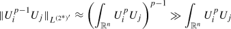
holds, while for \(n=6\) we have

and none of these estimates suffices to conclude the proof.
The fact that \(\int [(W+\rho )^{2^*}-W^{2^*}-2^*W^p\rho ] \ge 0\) is crucial to fix the issue in the proof of [9, Theorem 1.3].


References
Alexandrov, A.D.: A characteristic property of spheres. Ann. Mat. Pura Appl. 58(1), 303–315, 1962
Allegretto, W.: Principal eigenvalues for indefinite-weight elliptic problems in \({\mathbb{R}}^n\). Proc. Am. Math. Soc. 116(3), 701–706, 1992
Aubin, T.: Problemes isopérimétriques et espaces de Sobolev. J. Differ. Geom. 11(4), 573–598, 1976
Bahri, A.: Critical Points at Infinity in Some Variational Problems, vol. 182. Longman Scientific and Technical, London 1989
Bahri, A., Coron, J.-M.: On a nonlinear elliptic equation involving the critical Sobolev exponent: the effect of the topology of the domain. Commun. Pure Appl. Math. 41(3), 253–294, 1988
Bianchi, G., Egnell, H.: A note on the Sobolev inequality. J. Funct. Anal. 100(1), 18–24, 1991
Balinsky, A.A., Evans, W.D., Lewis, R.T.: The Analysis and Geometry of Hardy’s Inequality. Springer, Berlin 2015
Butscher, A.: A gluing construction for prescribed mean curvature. Pac. J. Math. 249(2), 257–269, 2011
Ciraolo, G., Figalli, A., Maggi, F.: A quantitative analysis of metrics on \(\mathbb{R}^n\) with almost constant positive scalar curvature, with applications to fast diffusion flows. Int. Math. Res. Not. 2018(21), 6780–6797, 2017
Ciraolo, G., Figalli, A., Maggi, F., Novaga, M.: Rigidity and sharp stability estimates for hypersurfaces with constant and almost-constant nonlocal mean curvature. Journal füur die reine und angewandte Mathematik (Crelles Journal)2018(741), 275–294, 2018
Cicalese, M., Leonardi, G.P.: A selection principle for the sharp quantitative isoperimetric inequality. Arch. Ration. Mech. Anal. 206(2), 617–643, 2012. https://doi.org/10.1007/s00205-012-0544-1. issn: 0003-9527
Ciraolo, G., Maggi, F.: On the shape of compact hypersurfaces with almost-constant mean curvature. Commun. Pure Appl. Math. 70(4), 665–716, 2017
De Giorgi, E.: Sulla proprieta isoperimetrica dell’ipersfera, nella classe degli insiemi aventi frontiera orientata di misura finita. In: Memoria di Ennio De Giorgi p. 198 (1958)
del Pino, M., Sáez, M.: On the Extinction Profile for Solutions of \(u_t= \Delta u^{(N- 2)/(N+ 2)}\). Indiana Univ. Math. J. 611–628 (2001)
Ding, W.Y.: On a conformally invariant elliptic equation on \({\mathbb{R}}^n\). Commun. Math. Phys. 107(2), 331–335, 1986
Delgadino, M.G., Maggi, F.: Alexandrov’s theorem revisited. Anal. PDE12(6), 1613–1642, 2019
Delgadino, M.G., Maggi, F., Mihaila, C., Neumayer, R.: Bubbling with L2-almost constant mean curvature and an Alexandrov-type theorem for crystals. Arch. Ration. Mech. Anal. 230.3, 1131–1177, 2018
Fusco, Nicola, Maggi, Francesco, Pratelli, A.: The sharp quantitative isoperimetric inequality. In: Annals of mathematics , pp. 941–980 (2008)
Figalli, A., Maggi, F., Pratelli, A.: A mass transportation approach to quantitative isoperimetric inequalities. Invent. Math. 182(1), 167–211, 2010
Gidas, B., Ni, W.-M., Nirenberg, L.: Symmetry and related properties via the maximum principle. Commun. Math. Phys. 68(3), 209–243, 1979
Maggi, F.: Some methods for studying stability in isoperimetric type problems. Bull. Am. Math. Soc. 45(3), 367–408, 2008
Morris, I.D.: A rapidly-converging lower bound for the joint spectral radius via multiplicative ergodic theory. Adv. Math. 225.6, 3425–3445, 2010
Machihara, S., Ozawa, T., Wadade, H.: Remarks on the Rellich inequality. Math. Z. 286(3–4), 1367–1373, 2017
Obata, M.: Certain conditions for a Riemannian manifold to be isometric with a sphere. J. Math. Soc. Jpn. 14(3), 333–340, 1962
Struwe, M.: Variational Methods: Applications to Nonlinear Partial Differential Equations and Hamiltonian Systems, vol. 34. Springer, Berlin 2008
Struwe, M.: A global compactness result for elliptic boundary value problems involving limiting nonlinearities. Math. Z. 187(4), 511–517, 1984
Szulkin, A., Willem, M.: Eigenvalue problems with indefinite weight. Stud. Math. 135, 191–201, 1995
Talenti, G.: Best constant in Sobolev inequality. Ann. Mat. pura Appl. 110(1), 353–372, 1976
Vázquez, J.L.: Smoothing and Decay Estimates for Nonlinear Diffusion Equations: Equations of Porous Medium Type, vol. 33. Oxford University Press, Oxford 2006
Wente, H.: Counterexample to a conjecture of H. Hopf. Pac. J. Math. 121(1), 193–243, 1986
Acknowledgements
both authors are funded by the European Research Council under the Grant Agreement No. 721675 “Regularity and Stability in Partial Differential Equations (RSPDE)”.
Author information
Authors and Affiliations
Corresponding author
Additional information
Communicated by F. Otto
Publisher's Note
Springer Nature remains neutral with regard to jurisdictional claims in published maps and institutional affiliations.
Appendices
Appendix A. Spectral Properties of the Weighted Laplacian
Let \(w\in L^{\frac{n}{2}}({\mathbb {R}}^n)\) be a positive weight. Our goal is to study the properties of the spectrum of the operator \(\frac{-\Delta }{w}\) and of its eigenfunctions. The spectrum of such a weighted Laplacian is thoroughly studied in literature, see for example [2]. An exhaustive list of related references is contained in the introduction of [27].
After some first basic statements that tell us that the spectrum of the operator is discrete, we move our attention to the properties of the eigenfunctions. For general weights we prove that almost-eigenfunctions are close to true eigenfunctions and that the eigenfunctions obey a concentration property.
Finally we focus on weights that decay at infinity as  . In this situation we are able to show some finer integrability properties of the eigenfunctions, and deduce that the restriction of an eigenfunction is close to an eigenfunction for the restriction of the weight.
1.1 A.1. Results Valid for any \(w\in L^{\frac{n}{2}}({\mathbb {R}}^n)\)
Let us begin with a technical, albeit important, proposition that gives us a compact embedding (in the style of the classical Sobolev embedding) from a homogeneous Sobolev space into a weighted space.
Proposition A.1
(Compact embedding in weighted space) Given a positive integer \(n\in {\mathbb {N}}\), let \(1\le p < n\) and \(q < p^*\) be two real numbers. For any positive weight \(w\in L^{(\frac{p^*}{q})'}({\mathbb {R}}^n)\), the following compact embedding holds:

Proof
Let us fix a real number R, and denote by \(B_R=B(0,R)\) the ball of radius R centered at the origin. Thanks to the chain of embeddings

it follows that

and therefore, applying the Rellich-Kondrakov theorem, it holds that

Let us define \(w_R:{\mathbb {R}}^n\rightarrow {\mathbb {R}}\) as
Since \(w_R\in L^\infty ({\mathbb {R}}^n)\), it holds that

and therefore (A.1) implies

Let us remark that Hölder and Sobolev inequalities imply that, for any \(g\in {\dot{W}}^{1,p}({\mathbb {R}}^n)\) and any Borel set \(E\subseteq {\mathbb {R}}^n\), it holds that

where \(\alpha :=(\frac{p^*}{q})'\) and \(C=C(n, p, q)\) is a constant.
Let us now fix a bounded sequence \((f_k)_{k\in {\mathbb {N}}}\subseteq {\dot{W}}^{1,p}({\mathbb {R}}^n)\). Up to extracting a subsequence, thanks to (A.2), by a diagonal argument we can find a function \(f\in {\dot{W}}^{1, p}({\mathbb {R}}^n)\) such that for any \(R > 0\) it holds \(f_k\rightarrow f\) in the \(L^q_{w_R}(B_R)\)-norm. We want to prove that \(f_k\rightarrow f\) in the stronger \(L^q_w({\mathbb {R}}^n)\)-norm.
For a fixed \(R>0\), recalling (A.3), we have

The desired convergence now follows sending R to infinity. \(\quad \square \)
We can now state and prove the main theorem of this section.
Theorem A.2
For any \(n\ge 3\) and any positive weight \(w\in L^{\frac{n}{2}}({\mathbb {R}}^n)\), the inverse operator \(\left( \frac{-\Delta }{w}\right) ^{-1}\) is well-defined and continuous from \(L^2_w({\mathbb {R}}^n)\) into \(H^1({\mathbb {R}}^n)\). Hence, thanks to Proposition A.1, it is a compact self-adjoint operator from \(L^2_w({\mathbb {R}}^n)\) into itself.
Proof
Let \(\varphi \in H^1({\mathbb {R}}^n)\) and \(f\in L^2_w({\mathbb {R}}^n)\). Applying Hölder and Sobolev inequalities, we obtain

As a consequence, the map
is continuous and injective. Applying Riesz Theorem, it follows that there exists a unique continuous linear map \(T:L^2_w({\mathbb {R}}^n)\rightarrow H^1({\mathbb {R}}^n)\) such that for any \(f\in L^2_w({\mathbb {R}}^n)\) and any \(g\in H^1({\mathbb {R}}^n)\) it holds that
Thus \(T=\left( \frac{-\Delta }{w}\right) ^{-1}\) and the statement is proven. \(\quad \square \)
Remark A.3
From now on we will use implicitly the following useful identity:
Since we have shown that \(\left( \frac{-\Delta }{w}\right) ^{-1}\) is compact and self-adjoint, we know that its spectrum is discrete. From now on we move our attention to the structure of its eigenfunctions. We begin by showing that if a function is almost an eigenfunction, than it close to a true eigenfunction.
Lemma A.4
(Approximate eigenfunction) Let us fix \(n\ge 3\) and a positive weight \(w\in L^{\frac{n}{2}}({\mathbb {R}}^n)\). Let \(\psi \in L^2_w({\mathbb {R}}^n)\) be such that \(-\Delta \psi - \lambda w\psi = f\) for some \(\lambda > 0\) and \(f:{\mathbb {R}}^n\rightarrow {\mathbb {R}}\). If \(\psi = \sum \alpha _k\psi _k\) where \((\lambda _k^{-1},\psi _k)_{k\in {\mathbb {N}}}\) is the sequence of eigenvalues and normalized eigenfunctions for \(\left( \frac{-\Delta }{w}\right) ^{-1}\), then it holds that

Proof
Substituting \(\psi = \sum \alpha _k\psi _k\) into \(-\Delta \psi - \lambda w\psi = f\) yields
Applying \(\left( \frac{-\Delta }{w}\right) ^{-1}\) to both sides yields
and the desired inequality follows taking the \(L^2_w\)-norm. \(\quad \square \)
The following lemma ensures that, as soon as we assume natural conditions on the spectral decomposition of f, if \(-\Delta u-\lambda wu=f\) then we can control the \(H^1\)-norm of u with the \(H^{-1}\)-norm of f.
Lemma A.5
Let us fix \(n\ge 3\) and a positive weight \(w\in L^{\frac{n}{2}}({\mathbb {R}}^n)\). Let \(u\in L^2_w({\mathbb {R}}^n)\) and \(f\in H^{-1}({\mathbb {R}}^n)\) be such that \(-\Delta u-\lambda wu = f\) for some \(\lambda > 0\). Let \(u=\sum \alpha _k \psi _k\), where \((\lambda _k^{-1}, \psi _k)\) is the sequence of eigenvalues and normalized eigenfunctions of \(\left( \frac{-\Delta }{w}\right) ^{-1}\), and assume that whenever \(\alpha _k\not =0\) it holds \(\lambda _k\ge \lambda (1-\varepsilon )^{-1}\) for some \(\varepsilon \in \left( 0,\,1\right) \). Then

Proof
First of all, let us check that the family of functions \(\lambda _k^{-\frac{1}{2}}\psi _k\) is a complete orthonormal basis of \(H^1({\mathbb {R}}^n)\). For any \(i,j\in {\mathbb {N}}\), it holds
and thus the desired \(H^1\)-orthonormality follows from the orthonormality of \((\psi _k)\) with respect to the \(L^2_w\)-scalar product. A similar computation shows that this basis is also complete in \(H^1({\mathbb {R}}^n)\).
As shown in the proof of Lemma A.4, it holds that
and thus, since \(\lambda _k^{-\frac{1}{2}}\psi _k\) is an orthonormal basis of \(H^1({\mathbb {R}}^n)\), we deduce that

Similarly, it holds that

and thus the desired two-sided estimate follows directly from the assumption that \(\lambda _k\ge \lambda (1-\varepsilon )^{-1}\) whenever \(\alpha _k \ne 0\). \(\quad \square \)
It is natural to expect that the eigenfunctions are concentrated in the zone where the weight itself is concentrated. The following lemma shows exactly this.
Lemma A.6
(Concentration of eigenfunctions) Let us fix \(n\ge 3\) and a positive weight \(w\in L^{\frac{n}{2}}({\mathbb {R}}^n)\). Let \(\lambda >0\) and \(\psi \in L^2_w({\mathbb {R}}^n)\) be such that \(-\Delta \psi = \lambda w\psi \). For any measurable set \(E\subseteq {\mathbb {R}}^n\) it holds that

Proof
Hölder’s inequality gives us

Also, the fact that \(\psi \) is an eigenfunction relative to \(\lambda \) together with the Sobolev inequality tell us

where \(C=C(n)\) is a constant that depends only on the dimension.
Joining the two inequalities yields the desired estimate. \(\quad \square \)
1.2 A.2. Further Results When \(w\approx (1+|x|)^{-4}\)
If we assume more on the weight, namely that  , we can obtain some better integrability of the eigenfunctions and we can prove that, in a certain sense, the restriction of eigenfunctions for the weight \(w\) are eigenfunctions for the restriction of the weight.
In this section it is crucial that  , as we rely on Theorem A.7. This result is known in literature as Rellich’s inequality (see [7, Chapter 6]). A short proof of the mentioned inequality with the sharp constant can be found for example in [23].
Theorem A.7
(Rellich’s Inequality) If \(n\ge 5\) it holds that

for any \(f\in H^2({\mathbb {R}}^n)\), where \(H^2({\mathbb {R}}^n)\) is the space of functions with Laplacian in \(L^2({\mathbb {R}}^n)\).
Corollary A.8
Let \(w\in L^{\frac{n}{2}}({\mathbb {R}}^n)\) be a positive weight such that  for a constant \(c>0\) and some points \(x_1,\dots ,x_k\in {\mathbb {R}}^n\). If \(n\ge 5\), it holds that

for any function \(f\in L^2({\mathbb {R}}^n)\).
Proof
The statement is a direct consequence of Theorem A.7. \(\quad \square \)
We can now prove that the eigenfunctions of \(\frac{-\Delta }{w}\) are in \(L^2({\mathbb {R}}^n)\). A priori we know only that they belong to \(L^2_w({\mathbb {R}}^n)\). The proof is achieved by duality applying Corollary A.8.
Lemma A.9
Let \(w\in L^{\frac{n}{2}}({\mathbb {R}}^n)\) be a positive weight such that  for a constant \(c>0\) and some points \(x_1,\dots , x_k\in {\mathbb {R}}^n\). If \(n\ge 5\) and \(\psi \in L^2_w({\mathbb {R}}^n)\) is such that \(-\Delta \psi = \lambda w\psi \) for some \(\lambda >0\), then

Proof
Let us fix a test function \(\varphi \in C^{\infty }_c({\mathbb {R}}^n)\). It holds that

where in the last step we applied Corollary A.8. The statement follows by taking the supremum over all functions \(\varphi \) with  . \(\quad \square \)
Let us conclude our study of the spectral properties of \(\left( \frac{-\Delta }{w}\right) ^{-1}\) with the following intuitive proposition. It states that, under suitable assumptions, if we restrict an eigenfunction relative to the weight \(w\) to a zone where \(w\) is almost the same as \(w_1\), then the restriction is almost an eigenfunction for the weight \(w_1\).
Proposition A.10
For a fixed \(n\ge 5\), let \(w_1, w\in L^{\frac{n}{2}}({\mathbb {R}}^n)\) be two positive weights such that  and
and  for some constant \(c>0\) and \(\bar{x}\in {\mathbb {R}}^n\). Let \(\psi \in L^2_w({\mathbb {R}}^n)\) and \(\lambda >0\) be such that \(-\Delta \psi -\lambda w\psi = 0\) and \(\int _{{\mathbb {R}}^n} \psi ^2w=1\).
Let us fix an arbitrary smooth function \(\eta :{\mathbb {R}}\rightarrow \left[ 0,\,1\right] \) such that \(\eta (t)=1\) if \(t\le 1\) and \(\eta (t)=0\) if \(t\ge 2\). We will consider  universal constants (in particular they can be hidden in the \(\lesssim \) notation).
For a fixed radius \(R>1\), denote  , and write \(\varphi =\sum \alpha _k\varphi _k\) where \((\lambda _k^{-1},\varphi _k)\) is the sequence of eigenvalues for \(\left( \frac{-\Delta }{w_1}\right) ^{-1}\). Then it holds that

Proof
Without loss of generality we can assume \({{\bar{x}}} = 0\). For notational simplicity, we denote  .
.
Applying Lemma A.4 and Corollary A.8 we deduce that

Let us expand \(-\Delta \varphi -\lambda w_1\varphi \) as follows:
Since  and
and  , (A.4) and (A.5) imply

Given that \(\psi \) is an eigenfunction with unit \(L^2_w\)-norm, it holds  . Recalling that
  , a direct application of Lemma A.6 yields

Finally the last term is estimated as

Substituting all the mentioned estimates into (A.6) finishes the proof. \(\quad \square \)
Appendix B. Integrals Involving Two Talenti Bubbles
This appendix is devoted to the computations of integral quantities involving two Talenti bubbles. First we deal with the case of two general Talenti bubbles U and V, and integrals of the form \(\int _{{\mathbb {R}}^n} U^\alpha V^\beta \) with \(\alpha +\beta =2^*\). Then we consider the special case of two bubbles \(U=U[-Re_1,1]\) and \(V=U[Re_1,1]\) for a large \(R>1\) and we obtain a simple formula to compute very general integrals of functions that depend only on U and V.
Even though the estimate Proposition B.2 shares the same spirit of the estimates [4, F7–F21], our estimate is, as far as we can tell, not implied by the inequalities stated in [4].
All the proofs in this appendix exploit the same simple strategy: splitting the involved integrals in regions where the integrand has a power-like behavior and then computing the integrals explicitly.
Lemma B.1
Given \(n\ge 3\), let us fix \(\alpha +\beta =2^*\) with \(\alpha ,\beta \ge 0\), \(\lambda \in \left( 0,\,1\right] \), and \(z\in {\mathbb {R}}^n\). Set  .
.
If  for some \(\varepsilon >0\), then
If instead \(\alpha =\beta =\frac{2^*}{2}\), then
Proof
We split the proof in two cases (Figure 1 and Figure 2).
The case\(D\le \lambda ^{-1}\). In \(B(0,2\lambda ^{-1})\) it holds that \(U[z,\lambda ]\approx U[z,\lambda ](z) \approx \lambda ^{\frac{n-2}{2}}\), while in \(B(0,2\lambda ^{-1})^{\complement }\) it holds that  and
and  . Thus, recalling that \(\alpha +\beta =2^*\), we get
Let us approximate the value of such expression under a further assumption on the relation between \(\alpha \) and \(\beta \).
If \(\alpha \ge \beta +\varepsilon \), the expression becomes comparable to \(\lambda ^{\frac{n-2}{2}\beta }\).
If \(\beta \ge \alpha +\varepsilon \), the expression becomes comparable to \(\lambda ^{\frac{n-2}{2}\alpha }\).
If \(\alpha =\beta \), the expression becomes comparable to \(\lambda ^{\frac{n}{2}}\log (\lambda ^{-1})\).

The balls B(0, 1), \(B(z,\lambda ^{-1})\), and \(B(0,2\lambda ^{-1})\), involved in the proof of the case \(D\le \lambda ^{-1}\)
The case\(D\ge \lambda ^{-1}\).

The balls B(0, 1), \(B(0,\frac{D}{2})\), \(B(z,\lambda ^{-1})\), \(B(z,\frac{D}{2})\), and B(0, 2D), involved in the proof of the case \(D\ge \lambda ^{-1}\)
Since we know a priori that \(\lambda \le 1\), in this case we have also \(D\ge 1\). Then, in \(B(0,\frac{D}{2})\) we have
and similarly in \(B(z, \frac{D}{2})\) we have
We note that actually both approximations still hold inside \(B(0,2D)\setminus \left( B(0,\frac{D}{2})\cup \right. \left. B(z,\frac{D}{2})\right) \), whereas in \(B(0,2D)^{\complement }\) we have

Thanks to these approximations, we can compute
Once again, we approximate the value of such expression under a further assumption on the relation between \(\alpha \) and \(\beta \) (Fig. 2).
If \(\alpha \ge \beta +\varepsilon \), the expression becomes comparable to \((\lambda D^2)^{-\frac{(n-2)\beta }{2}}\).
If \(\beta \ge \alpha +\varepsilon \), the expression becomes comparable to \((\lambda D^2)^{-\frac{(n-2)\alpha }{2}}\).
If \(\alpha = \beta \), since \(D\lambda \ge 1\) and \(\lambda \le 1\) the expression becomes comparable to \(\log (D)\,(\lambda D^2)^{-\frac{n}{2}}\approx \log (\lambda D^2)\,(\lambda D^2)^{-\frac{n}{2}}\).
As we have covered all possible cases, the statement is proven. \(\quad \square \)
Proposition B.2
Given \(n\ge 3\), let \(U=U[z_1, \lambda _1]\) and \(V=U[z_2, \lambda _2]\) be two bubbles such that \(\lambda _1\ge \lambda _2\). Let us define the quantity \(Q=Q(U, V)=Q(z_1, \lambda _1, z_2, \lambda _2)\) as

Then, for any fixed \(\varepsilon >0\) and any nonnegative exponents such that \(\alpha +\beta =2^*\), it holds that

Proof
Since the integral \(\int _{{\mathbb {R}}^n} U^\alpha V^\beta \) is invariant under the transformations described in Section 2.1, this result follows directly from Lemma B.1. \(\quad \square \)
Remark B.3
The behavior of \(\int _{{\mathbb {R}}^n} U^\alpha V^\beta \) when \(\alpha \) is close, but not equal, to \(\beta \) cannot be captured by simple formulas as the ones in the statement of Proposition B.2. Indeed in such a range of exponents there is the transition between a pure power behavior and a power+logarithm behavior.
Corollary B.4
Given \(n\ge 3\) and two bubbles \(U_1=U[z_1, \lambda _1]\) and \(U_2=U[z_2, \lambda _2]\) with \(\lambda _1\ge \lambda _2\), it holds that
Proof
Thanks to the symmetries described in Section 2.1, without loss of generality we can assume \(z_1=0\), \(\lambda _1=1\). For clarity, let us denote \(\lambda :=\lambda _2\) and \(z:=z_2\).
Since \(\lambda \le 1\), it holds that \(U_2(0)\approx U_2(x)\) for any \(x\in B(0,1)\). Hence, we have

Thanks to Proposition B.2 we know that

so the statement is proven, since

\(\quad \square \)
Proposition B.5
Given \(n\ge 3\), let \(\varphi :\left( 0,\,\infty \right) ^2\rightarrow \left( 0,\,\infty \right) \) be a function such that
\(\varphi (x, y)\approx x^ay^b\) if \(y\le 2x\);
\(\varphi (x, y)\approx x^cy^d\) if \(x\le 2y\),
where \(a,b,c,d\ge 0\) are nonnegative exponents satisfying \(a+b=c+d>\frac{n}{n-2}\). If we denote \(U:=U[-Re_1, 1]\) and \(V:=U[Re_1, 1]\) for some \(R\gg 1\), then it holds that
where the hidden constants do not depend on R (but are allowed to depend on the dimension n and the function \(\varphi \)). As a consequence, it holds that
Proof
The only properties of U[0, 1] we are going to use are that \(U[0,1]\approx 1\) in B(0, 1) and  elsewhere.
We split the desired integral in four zones
where \(B_U = B(-Re_1, \frac{R}{2})\) and \(B_V=B(R e_1, \frac{R}{2})\). Let us compute the four terms separately.
We start with the integral on \(B_U\):
Of course, we can perform an analogous computation also on the ball \(B_V\).
In \(B(0, 2R)\setminus (B_U\cup B_V)\) it holds \(U\approx V\approx R^{-(n-2)}\) and thus \(\phi (U,V)\approx R^{-(a+b)(n-2)}\). Therefore
Finally, outside B(0, 2R) it holds that

Combining all these estimates, the result follows. \(\quad \square \)
Rights and permissions
About this article

Cite this article
Figalli, A., Glaudo, F. On the Sharp Stability of Critical Points of the Sobolev Inequality. Arch Rational Mech Anal 237, 201–258 (2020). https://doi.org/10.1007/s00205-020-01506-6
Received:
Accepted:
Published:
Issue Date:
DOI: https://doi.org/10.1007/s00205-020-01506-6