
Abstract
This article introduces the new class of continuous set covering problems. These optimization problems result, among others, from product portfolio design tasks with products depending continuously on design parameters and the requirement that the product portfolio satisfies customer specifications that are provided as a compact set. We show that the problem can be formulated as semi-infinite optimization problem (SIP). Yet, the inherent non-smoothness of the semi-infinite constraint function hinders the straightforward application of standard methods from semi-infinite programming. We suggest an algorithm combining adaptive discretization of the infinite index set and replacement of the non-smooth constraint function by a two-parametric smoothing function. Under few requirements, the algorithm converges and the distance of a current iterate can be bounded in terms of the discretization and smoothing error. By means of a numerical example from product portfolio optimization, we demonstrate that the proposed algorithm only needs relatively few discretization points and thus keeps the problem dimensions small.
1 Introduction
Continuous set covering problems describe the task to cover a given compact set \(Y \subset {\mathbb {R}}^m\) with a fixed number of adjustable objects, which themselves are compact subsets of \({\mathbb {R}}^m\). The objects depend on a parameter vector that can for example encode information about their size or location. If the objects are associated with some cost function on the parameter vector, the goal is to find a configuration of objects such that Y is covered and the cost is minimized. The following definition of the continuous set covering problem represents this task in a set-theoretic formulation. We consider two compact sets \(X \subset {\mathbb {R}}^n\) and \(Y\subset {\mathbb {R}}^m\) (\(n, m\in {\mathbb {N}}\)). For a given number \(N\in {\mathbb {N}}\) and all \({\mathbf {x}}\in X\), let \(P_i({\mathbf {x}}) \subset {\mathbb {R}}^m\), \(i = 1, \dots , N\), be compact sets parameterized by \({\mathbf {x}}\). Further, let \(f: {\mathbb {R}}^n \rightarrow {\mathbb {R}}\) be a continuous cost function. Then, the continuous set covering problem (CSCP) is given by
Throughout this article, we assume that in any instance of CSCP (1), beyond being compact, the set Y has infinite cardinality, \(|Y| = \infty \). Furthermore, the compact sets \(P_i({\mathbf {x}})\), \(i = 1, \dots , N\) have a functional description, i.e.
where \(p_i \in {\mathbb {N}}\) for \(i = 1, \dots , N\), and the given functions \( g_{ij}: {\mathbb {R}}^n \times {\mathbb {R}}^m \rightarrow {\mathbb {R}}\) are continuously differentiable. Figure 1 depicts the constraint (1b) for an instance of CSCP where four parameterized objects cover a rectangle in \({\mathbb {R}}^2\).

Continuous set covering task: Four parameterized objects \(P_1({\mathbf {x}}), \dots , P_4({\mathbf {x}})\) should cover the rectangle Y in \({\mathbb {R}}^2\)
For the classical discrete set covering problem as defined by Garey and Johnson (1990) a finite set is considered. The goal is to determine, if this set can be covered by a fixed number of subsets which are chosen from a given collection. According to Karp (1972) this problem remains NP-complete even if all subsets in the collection consist of at most three elements. The continuous set covering problem as introduced above differs in two ways from the classical discrete set covering problem: First, the set to be covered Y and the covering sets \(P_i({\mathbf {x}}), i=1, \dots , N\) have infinite cardinality. Second, the covering sets are parameterized by a real-valued vector \({\mathbf {x}}\in X\).
From a mathematical point of view, many special cases of (1) are well known and thus much literature exists. The task of covering a continuous polygonal set by one ellipsoid for example is solved by so-called minimum volume or Löwner-John ellipsoids (see Gruber (2011) among others). An often considered geometric problem is minimal ball covering, which appears in literature under different names such as disc covering or sprinkler problem in the two dimensional case. Different to the minimum volume covering ellipsoid problem, minimal ball covering usually comprises more than one covering object. Exemplary specifications of these problems can be found in Jandl and Wieder (1988), Melissen and Schuur (2000), Galiev and Karpova (2010), Kiseleva et al. (2009). The mathematical problem that comes closest to (1) is given by Stoyan et al. (2011). The authors aim at covering a polygonal region by a certain number of rectangles that can be moved in the plane. The applications behind this problem are query optimization in spatial databases or shape recognition for robotics. Stoyan et al. (2011) formulate the problem as a feasibility problem. Using \(\Phi \)-function techniques Bennell et al. (2010) end up with a covering constraint criterion that—although they do not state this—resembles a semi-infinite constraint.
Problem instances of CSCP are suited to formulate certain product portfolio design tasks that arise for example in engineering contexts. Optimal product portfolio design, also known as product line or product family design, comprises an important issue a company has to deal with: It is the task of deciding which and how many products to produce and offer its customers. A conflict in this task is to satisfy as many customers with high-quality products versus keeping production, storage, or maintenance costs and thus portfolio size, low. The first to introduce the problem of optimal product portfolio design were Green and Krieger (1985). They defined a product as a combination of certain components, each of which could be chosen from a finite selection. The resulting task is a linear optimization problem with binary decision variables. Due to its combinatorial complexity, the problem was early proven to be NP-hard by Kohli and Krishnamurti (1989).
Depending on the specific task, the problem was reformulated as mixed-integer combinatorial optimization problem by Jiao and Zhang (2005), bi-level problem by Du et al. (2014) and as multiobjective optimization problem by Du et al. (2019). The variety of solution approaches ranges from the application of branch-and-bound-method by van den Broeke et al. (2017) over evolutionary approaches by van den Broeke et al. (2017) and Du et al. (2019) as well as their combinations with some heuristic by Jiao et al. (2007) to data-driven decision tree classification in Tucker and Kim (2009).
All these problems have in common that they aim at designing product portfolios for discrete sets of customer demands. Further, the attributes of the products are selected among sets of discrete options. Tsafarakis et al. (2013) state that in real life, many product attributes are described in terms of continuous, real numbers such as weight, length, speed, capacity, power, energy and time. The authors therefore consider product portfolio optimization problems with continuous decision variables. Selecting only few characteristic values in a possible interval of attribute realizations constitutes a very restrictive assumption, which on one hand may reduce the problem’s complexity, but on the other hand may also lead to less than optimal solutions. The new problem class CSCP (1) introduced in this article allows us to consider real-valued decision variables but also continuous sets of costumer demands that are to be covered.
While Tsafarakis et al. (2013) look at the optimization of a portfolio of industrial cranes, these arguments directly transfer to other engineering portfolio optimization tasks, such as optimizing the portfolio of machines. The sets \(P_i({\mathbf {x}})\), \(i = 1, \dots , N\) in this case represent the so-called operation areas of the machines. As the name suggests, these areas comprise the sets of all points at which the machines can be operated. With regard to that, in Fig. 1 the operation areas of four transport pumps are sketched, see also Sect. 4 and Appendix A for more information on this application.
In this article the set-theoretic formulation of CSCP is not solved directly. In Sect. 2 we show that the problem has a straightforward reformulation as semi-infinite optimization problem (SIP). Semi-infinite optimization is a large research area. Being by no means exhaustive, we suggest Hettich and Kortanek (1993), López and Still (2007), Shapiro (2009) for comprehensive surveys on SIP. The monograph of Stein (2003) provides insights into the field via exploitation of the bi-level structure of SIPs. It turns out that the SIP associated with CSCP has an intrinsically difficult structure in that possible curvature properties of the basic functions \(g_{ij}\), \(j = 1, \dots , p_i\), \(i = 1, \dots , N\), get lost and the semi-infinite constraint function is not continuously differentiable, even if the basic functions are. Hence, the straightforward application of standard methods from semi-infinite programming is difficult. We therefore develop an algorithm that aims at finding approximate solutions for CSCP based on easier finite and smooth nonlinear optimization problems (NLPs). To do so we combine two techniques: Adaptive discretization of the infinite index set as introduced by Blankenship and Falk (1976) is coupled with approximation of the non-smooth functions by smooth ones. For the second step, it is of importance that the approximations converge uniformly, the approximation error is known and that convergence can be steered by some parameter. Background information of both approximating methods, as well as literature, is given in Sect. 2.
The article is structured as follows: Sect. 2 provides the solution approach of CSCP in form by means of a SIP. Further, the problem structure is analyzed and reasonable approximating problems are introduced. The topic of Sect. 3 is our algorithm based on adaptive discretization of the infinite index set and two variants of entropic smoothing of the non-smooth constraint function, and its associated convergence results. Section 4 provides some numerical studies on the algorithm’s performance. It further demonstrates, that the presented solution approach for CSCP is capable to find solutions for a certain product portfolio design task with continuously described products taking manageable effort. Finally, a conclusion is drawn (Sect. 5).
2 Solution approach: consider CSCP as SIP
There are no optimization algorithms available that can directly operate on CSCP in its set-theoretic formulation (1). However, given the functional description of the sets \(P_i({\mathbf {x}})\), \(i = 1, \dots , N\) in (2), CSCP can be equivalently formulated as standard semi-infinite optimization problem
Yet, the constraint function of \(\text {SIP}_\text {CSCP}\) (3),
is a min-max function. In general, such a function is not continuously differentiable everywhere, even if the basic functions \(g_{ij}\), \(j = 1, \dots , p_i\), \(i = 1, \dots , N\), are differentiable. The non-differentiable parts usually show up as "kinks" in the graph of the constraint function (Fig. 2). They occur at locations where the function values of at least two of the basic functions \(g_{ij}\), \(j = 1, \dots , p_i\), \(i = 1, \dots , N\), coincide and represent the values of g. Note that the non-differentiability occurs in both, the decision vector \({\mathbf {x}}\) and the index variables \({\mathbf {y}}\).
Another unpleasant characteristic of (4) is that the combination of minimum and maximum operator destroys any curvature property the basic functions might possess. Thus, for given \({\mathbf {y}} \in Y\), the covering constraint function in general is not convex in \({\mathbf {x}}\) and therefore, \(\text {SIP}_\text {CSCP}\) is a non-convex optimization problem and must be expected to possess multiple local extrema.
To check the feasibility of a candidate solution \({\mathbf {x}}\) of \(\text {SIP}_\text {CSCP}\) requires solving the so-called lower level problem of \(\text {SIP}_\text {CSCP}\)
to global optimality on \(Y\). However, the same arguments that attest non-convexity in \({\mathbf {x}}\) also provide that the constraint function is not concave in the index variable \({\mathbf {y}}\) for fixed \({\mathbf {x}}\). Figure 2 illustrates that the kinks caused by the min-max function result in a multi-extremal function structure. Together with its non-differentiability, this makes finding global solutions difficult. Therefore, checking the feasibility of a candidate solution for \(\text {SIP}_\text {CSCP}\) is already a challenging problem itself. Although this topic is worth to be further investigated, we will not go into further detail in this article.

Graph of the constraint function \(g({\mathbf {x}}, \cdot ) \) of a \(\text {SIP}_\text {CSCP}\) with \(N = 2\) for a fixed decision vector \({\mathbf {x}} \in X\). The two objects \(P_1({\mathbf {x}})\) and \(P_2({\mathbf {x}})\) are required to cover a rectangle (background) in \({\mathbb {R}}^2\) – the shown configuration thus is infeasible
To sum up, the structural properties induced by the combination of the \(\text {min}\) and \(\text {max}\) operator in the constraint function prevent the straightforward usage of direct solution methods for semi-infinite programs like the Reduction Ansatz, described for example in the review from Hettich and Kortanek (1993). Mitsos and Tsoukalas (2015) provide a global solution procedure for SIPs, which only requires continuity but not differentiability of the objective and constraint functions. Beyond the few requirements on structure, also the global solution part would be very attractive in view of the multi-extremality of \(\text {SIP}_\text {CSCP}\). However, the global solution of the problem \(\text {SIP}_\text {CSCP}\) with the available global solvers can be problematic. First, not all global optimization solvers can handle min and max operators directly. Such operators typically must be reformulated at the cost of additional auxiliary binary variables. As the min and max operators appear in the semi-infinite constraints this has to be done for every discretization point. This leads to a strong increase of the problem dimension. Second, the problem \(\text {SIP}_\text {CSCP}\) often contains a strong symmetry. If we try to cover a set Ywith multiple parametric bodies of the same shape, then each permutation of the covering bodies leads to the same solution. We therefore refrained from global solution approaches and turned to faster, local methods for NLPs. To be able to apply these methods, we implemented two possibilities to approximate the non-smooth \(\text {SIP}_\text {CSCP}\) by finite, smooth NLPs
2.1 Approximations of \(\text {SIP}_\text {CSCP}\)
Useful approximations for optimization problems ideally satisfy two goals: First, they should be easier to solve, either due their problem structure or due to the existence of suitable solution procedures. Second, the minimizers found for the approximating problems should, at least in their limits with respect to approximation quality, represent minimizers of the actual problem. This section focuses on the first goal, the set up of easier problems.
In this article, we focus on the successful approach of applying double entropic smoothing and a variant thereof to \(\text {SIP}_\text {CSCP}\). Thereby we end up with smooth approximation problems which come at the cost of having to steer two smoothing parameters. This can be tricky, as we discuss in Sect. 4. Yet, the size of the approximation problems (decision space and number of constraints) remains the same as that of the original problem. The double entropic smoothing is just one possibility to get approximation problems for \(\text {SIP}_\text {CSCP}\). An overview—that makes no claim to be complete—of other approximations and reformulations of \(\text {SIP}_\text {CSCP}\) is given in the thesis of Krieg (2020). There, it was found that non of the reformulations and approximations are for free. Depending on the underlying basic functions of a particular \(\text {SIP}_\text {CSCP}\) problem and the availability of optimization software, some might be more advantageous than others.
In a first step, we use what Hettich and Kortanek (1993) designate as the simplest way to approximate a SIP by a finite optimization problem: We replace the infinite index set Y by a finite set
consisting of \(r \in {\mathbb {N}}\) points. This results in the following finite nonlinear optimization problem:
Secondly, we apply regularization. This is a known means for tackling non-smooth functions in optimization. Further information on the method can be found for example in the articles of Bertsekas (1975) and Chen (2012). Applying regularization methods to non-smooth optimization problems yields parametric optimization problems. Their approximation quality ideally can be measured in terms of the regularization parameters.
The regularization functions of our choice are so-called entropic smoothing functions. They were employed by Li (1994), Chen and Templeman (1995), Li and Fang (1997), Xu (2001), or Polak et al. (2003) in minimax optimization, for example. A similar function, called cross-entropy was used by Zhang et al. (2009) and Ruopeng (2009) to approximate the Lagrangian function of a minimax problem. In all these cases, only one max operator had to be replaced by the regularization function to get a smooth approximation. For the constraint function (4), we use the double entropic smoothing approach for min-max functions that couples entropic smoothing with a result of Schwientek (2013) who shows that a likewise function can also be used to approximate a pointwise minimum of finitely many functions. We found this approach also in an article of Tsoukalas et al. (2009) who reduce an unconstrained, finite min-max-min problem to the task of minimizing a smooth function. The authors then use a steepest descent algorithm to solve the resulting parametric optimization problems. The latter is not directly applicable to our constrained optimization problem. Further, the semi-infinite nature of \(\text {SIP}_\text {CSCP}\) makes additional actions with respect to the infinite number of constraints necessary.
In addition to the basic double entropic smoothing, we look at a second variant of these regularization functions. By replacing the constraint function in (6) with either the double entropic smoothing function \(g^{s, t}\) or the shifted entropic smoothing function \({\tilde{g}}^{s, t}\) (definitions below), we get the following parametric but smooth and finite NLPs:
2.1.1 The entropic smoothing-based regularization functions
Parameterized by \(s < 0\) and \(t > 0\), the double entropic smoothing function is given by
As the following results show, the double entropic smoothing function obeys monotonicity with respect to the smoothing parameters and converges uniformly to the min-max function g. Interested readers find the corresponding proofs in Appendix B.
Lemma 1
The family of double entropic smoothing functions \(\{g^{s, t}\}_{s, t}\) with \(s < 0\) and \(t > 0\) is monotonically decreasing in (|s|, t).
The next result states the smoothing error that measures the distance between the double entropic smoothing function and the function it approximates and can thus be used to steer approximation quality.
Lemma 2
For arbitrary parameters \(s < 0\) and \(t > 0\) and any \({\mathbf {x}} \in {\mathbb {R}}^n\), \({\mathbf {y}} \in {\mathbb {R}}^m\),
holds.
Remark 1
Note that the double entropic smoothing function is d-times continuously differentiable, if all the basic functions \(g_{ij}\), \(j = 1, \dots , p_i\), \(i = 1, \dots , N\), that define the min-max function g, are d-times differentiable.
Translating the double entropic smoothing functions downwards by the smoothing error, given in (10), yields the shifted entropic smoothing function.
The shifted entropic smoothing function is monotonically increasing in (|s|, t) for \(s < 0\) and \(t > 0\), as stated and proven in Lemma 4 in Appendix B. Due to the substracted smoothing error, it approximates the min-max function from below. Finally, the shifted entropic smoothing function also converges uniformly.
Sequences of regularization functions. In our solution procedure for \(\text {SIP}_\text {CSCP}\), we will make use of sequences of successively better approximations. Thus, we consider families of functions of either smoothing type defined by sequences of parameters \(\{(s_k, t_k)\}_{k \in {\mathbb {N}}_0}\) with \(s_k < 0\) and \(t_k > 0\) for all \(k \in {\mathbb {N}}\). Supposing that both parameter sequences are monotonous and divergent with \(s_k \rightarrow -\infty \) and \(t_k \rightarrow \infty \), as \(k \rightarrow \infty \), from Lemmas 1 to 2, the following properties can be derived for the families of functions: The functions of the family of double entropic smoothing functions \(\{g^{s_k,t_k}\}_{k \in {\mathbb {N}}_0}\) bound the min-max function g from above, whereas the family of shifted entropic smoothing functions \(\{{\widetilde{g}}^{s_k, t_k}\}_{k \in {\mathbb {N}}_0}\) is a family of lower bounds. Both sequences of functions converge uniformly to the min-max function as \(k \rightarrow \infty \). Lemma 2 provides us with a smoothing error for these sequences of functions, in that
holds with
For the interpretation of approximating solutions and their feasibility with respect to the actual problem, it is useful to investigate the feasible sets of the problems and their relations.
2.2 Feasible sets
To begin with, let us state that regularization of the constraint function is independent of the index set and thus can already be applied to \(\text {SIP}_\text {CSCP}\). For the two entropic smoothing-based regularization functions, this yields the following smooth SIPs
and
In the following, the feasible set of \(\text {SIP}_\text {CSCP}\) is denoted by \(M\). The feasible sets of the regularization-based approximating problems (13) and (14) are indicated by \(M^{s, t}\) and \({\widetilde{M}}^{s, t}\). Whenever discretizations are considered, the feasible sets get the argument \(({\dot{Y}})\). The feasible sets of the problems with both approximation types combined, (7) and (8), are abbreviated in a straightforward manner by \(M^{s, t}({\dot{Y}})\) and \({\widetilde{M}}^{s, t}({\dot{Y}})\), respectively. Further, from now on, we look at sequences of approximation problems and explain that, under certain conditions, they become successively better approximations for \(\text {SIP}_\text {CSCP}\).
Discretization. Let \(\{{\dot{Y}}_k\}_{k \in {\mathbb {N}}_0}\) be a sequence of finite subsets of the infinite index set Y. Further, assume that the sequence is monotonically increasing with respect to set inclusion, i.e. \({\dot{Y}}_{k}\subseteq {\dot{Y}}_{k + 1}\) for all \(k \in {\mathbb {N}}_0\). Then, the problems \(\text {SIP}_\text {CSCP}({\dot{Y}}_k)\) form subsequently better outer approximations of \(\text {SIP}_\text {CSCP}\), i.e. their feasible sets are ordered with respect to set inclusion as follows: For all \(k \in {\mathbb {N}}_0\) it holds that
Regularization. Let \(\{(s_k, t_k)\}_{k \in {\mathbb {N}}_0}\) be a sequence of smoothing parameters with the property that for all \(k \in {\mathbb {N}}_0\), \(s_k < 0\) and \(t_k > 0\) holds. Further suppose that both parameter sequences are divergent and monotonically increasing in their absolute values. The following result is formulated using the notion of set convergence and set limits in the sense of Kuratowski-Painlevé. The corresponding definitions can be found in the book of Rockafellar and Wets (2009).
Proposition 1
For all \(k \in {\mathbb {N}}_0\), the following statements hold
-
1.
\(M^{s_{k}, t_{k}}\) is closed.
-
2.
\({\widetilde{M}}^{s_{k}, t_{k}}\) is closed.
-
3.
The sequence of feasible sets \(\{M^{s_{k}, t_{k}}\}_{k \in {\mathbb {N}}_0}\) is monotonically increasing with respect to set inclusion.
-
4.
\(M^{s_{k}, t_{k}} \subseteq M\) for all \(k \in {\mathbb {N}}_0\).
-
5.
The sequence of feasible sets \(\{{\widetilde{M}}^{s_{k}, t_{k}}\}_{k \in {\mathbb {N}}_0}\) is monotonically decreasing with respect to set inclusion.
-
6.
\({\widetilde{M}}^{s_{k}, t_{k}} \supseteq M\) for all \(k \in {\mathbb {N}}_0\).
-
7.
\(\lim _{k \rightarrow \infty }{\widetilde{M}}^{s_{k}, t_{k}} = M\).
Proof
The closedness of the feasible sets of the approximating problems is given by the fact that sublevel sets of continuous functions are closed and the two types of regularization functions (9) and (11) are continuous, because the functions \(g_{ij}\) are continuous, for all \(i = 1, \dots ,N, j = 1, \dots , p_i\) by assumption.
Statements 3 and 4 are grounded on the monotonicity of the double entropic smoothing with respect to the considered sequence of smoothing parameters (Lemma 1): For all \(k \in {\mathbb {N}}_0\) and all \(({\mathbf {x}}, {\mathbf {y}}) \in X\times Y\), it holds that
The same argument applies to statements 5 and 6 for the feasible sets of the problems based on shifted entropic smoothing in reverse ordering.
Statement 7 holds true if the set of all limit points of the sets \({\widetilde{M}}^{s_{k}, t_{k}}\), \(k \in {\mathbb {N}}_0\) equals the set of all cluster points of the sets \({\widetilde{M}}^{s_{k}, t_{k}}\) and both are equal to \(M\).
By statement 6, we have that
Hence, we need to show that \(\limsup _{k\rightarrow \infty } {\widetilde{M}}^{s_{k}, t_{k}} \subseteq M\) holds. To do so, for \({\bar{{\mathbf {x}}}} \in \limsup _{k\rightarrow \infty }{\widetilde{M}}^{s_{k}, t_{k}}\), consider a sequence of points \(\{{\mathbf {x}}^{k_l}\}_{l \in {\mathbb {N}}_0}\), \({\mathbf {x}}^{k_l} \in {\widetilde{M}}^{s_{k_l}, t_{k_l}}\) for all \(l \in {\mathbb {N}}_0\), that converges towards \({\bar{{\mathbf {x}}}}\). Next we make use of continuity of the functions \(g(\cdot , {\mathbf {y}})\) on X for all \({\mathbf {y}} \in Y\), feasibility of the points \({\mathbf {x}}^{k_l}\) for the corresponding approximating problem, and uniform convergence of the shifted entropic smoothing function. Then, for all \({\mathbf {y}} \in Y\), we have
Hence, \({\bar{{\mathbf {x}}}} \in M\) holds. \(\square \)
Statements four and six of Proposition 1 state that regularization based on double entropic smoothing leads to inner approximations of \(\text {SIP}_\text {CSCP}\), i.e. these problems are stricter than the original problem. In contrast to this, regularizations with shifted-entropic smoothing yield outer approximations, i.e. relaxed problems.
For the problems \(\text {SIP}_\text {CSCP}\) and their shifted entropic smoothing-based approximations, the convergence of the feasible sets given in statement 7 of Proposition 1 is equivalent to epiconvergence of the sequence of problems \(\{\widetilde{\text {SIP}}_\text {CSCP}^{s_{k}, t_{k}}\}_{k\in {\mathbb {N}}_0}\) towards \(\text {SIP}_\text {CSCP}\). The concept of epiconvergence was used by Polak (1997) to show that the minimizers of approximating problems in the limit represent the minimizers of the actual problem. The feasible sets of a sequence of problems of type \(\text {SIP}_\text {CSCP}^{s, t}\) does not converge towards the feasible set of \(\text {SIP}_\text {CSCP}\) in general. The reason for this are points on the boundary of the feasible set, that can never be reached by these so-called inner approximations. To ensure convergence of minimizers of double entropic smoothing-based approximations towards minimizers of \(\text {SIP}_\text {CSCP}\), we have to require additional structure from \(\text {SIP}_\text {CSCP}\). We will return to this issue in Sect. 3.
Discretization and Regularization. Under the same assumptions on the sequences of discretization sets \(\{{\dot{Y}}\}_{k \in {\mathbb {N}}_0}\) and the sequences of smoothing parameters \(\{(s_k, t_k)\}_{k \in {\mathbb {N}}_0}\) as in the previous paragraphs, we can retrieve some interesting properties of the feasible sets of the approximating problems (7) and (8).
Proposition 2
-
1.
The sequence of feasible sets \(\left\{ \right. {\widetilde{M}}^{s_{k}, t_{k}}({\dot{Y}}_{k})\left. \right\} _{k \in {\mathbb {N}}_0}\) is monotonically decreasing with respect to set inclusion.
-
2.
\({\widetilde{M}}^{s_{k}, t_{k}}({\dot{Y}}_{k})\) \(\supseteq M\) for all \(k \in {\mathbb {N}}_0\).
-
3.
\({\widetilde{M}}^{s_{k}, t_{k}}\) \(\subseteq \) \({\widetilde{M}}^{s_{k}, t_{k}}({\dot{Y}}_{k})\) for all \(k \in {\mathbb {N}}_0\).
-
4.
\(M^{s_{k}, t_{k}}\) \(\subseteq \) \(M^{s_{k}, t_{k}}(\dot{Y_{k}})\) for all \(k \in {\mathbb {N}}_0\).
Proof
The proofs of the first and second statement are combinations of (15) and Proposition 1, statements 5 and 6, respectively. The third and fourth statements are obvious, as discretization of the infinite index set leads to a relaxed problem, no matter which constraint function is considered. \(\square \)
Figure 3 depicts the relations between the feasible sets of \(\text {SIP}_\text {CSCP}\) and its different types of approximating problems for an example instance of the problem with two decision variables.

Relationship between feasible sets of CSCP and approximating problems
Note that the combination of regularization with double entropic smoothing (9) and discretization destroys the set-inclusion properties of either of the two approximation techniques: While discretization results in an outer approximation of a SIP, regularization of less-or-equal constraints by double entropic smoothing yields an inner approximation of the feasible set with respect to set inclusion. Thus, in general,
hold. This situation can be seen in the lower left panel of Fig. 3. The sequence of feasible sets \(\{ M^{s_{k}, t_{k}}(\dot{Y_{k}})\}_{k\in {\mathbb {N}}_0}\) must not even be monotonous. Nevertheless, we will see that this type of approximation can still be used for \(\text {SIP}_\text {CSCP}\) and the numerical study in Sect. 4 will show that it is worth to be used.
We think the insight gained into the relationships between the feasible sets of \(\text {SIP}_\text {CSCP}\) and its different types of approximating problems is of benefit for understanding the convergence results for the solution method presented in the following section.
3 An adaptive discretization and smoothing-based algorithm for \(\text {SIP}_\text {CSCP}\)
In this section, we present an algorithm that finds approximate solutions to \(\text {SIP}_\text {CSCP}\) by solving sequences of problems of type \(\text {SIP}_\text {CSCP}^{s, t}\) or \(\widetilde{\text {SIP}}_\text {CSCP}^{s, t}\), respectively. The main ingredients of the algorithm are adaptive discretization of the semi-infinte index set, as introduced by Blankenship and Falk (1976), and a strategy to update the parameters of double or shifted entropic smoothing, s and t, such that the approximating quality of the substitute problems becomes successively better.
Since its introduction in 1974, adaptive discretization formed the base of many solution methods for semi-infinite programs. We mention just a few to illustrate the range of concerns these methods focused on. Seidel and Küfer (2020), for example, combined adaptive discretization with bi-level techniques. Thereby, they could reach a quadratic rate of convergence under adequate problem structure. One inherent problem of all discretization methods was tackled by Tsoukalas and Rustem (2011): the approximate solutions usually are infeasible for the original SIP. To solve this problem, the authors enhanced the adaptive discretization method with a procedure to get \(\epsilon \)-optimal, but feasible solutions. This method was further extended by Djelassi and Mitsos (2017) in order to find global solutions of SIP. Adaptive discretization is also used in solution techniques for generalized semi-infinite programs. These problems provide difficulties for adaptive discretization methods as the infinite index set depends on the decision variables. This was overcome by Schwientek et al. (2020) by transforming the generalized SIP into a standard one whenever a new discretization point should be found. Mitsos and Tsoukalas (2015) developed a global solution method for generalized semi-infinite programs. In this method, they make use of adaptive discretization for defining bounding problems.
Our adaptive discretization and smoothing based-approach is stated in Algorithm 1. This variant aims at solving problems (7). By replacing line 3 with the alternative

the same procedure can also be applied to the outer approximations (8) of \(\text {SIP}_\text {CSCP}\). In this case, all problems considered in the algorithm are outer approximations and the requirement \(M^{s_{0}, t_{0}}\)\(\ne \emptyset \) is not needed.

All convergence results presented in Section 3.1 are essentially valid if the algorithm constructs and solves problems that become successively better approximations over the iterations. To guarantee these improvements, the realization of the algorithm must satisfy the following requirements, which we assume to hold for the remainder of the article.
Assumption 1
(Requirements on Algorithm 1)
-
1.
The discretization update criteria (step 4 of Algorithm 1) has to be chosen in such a way that it is dismissed only finitely often, if
$$\begin{aligned} g({\mathbf {x}}^{k+1},{\mathbf {y}}^{k+1})>0. \end{aligned}$$ -
2.
The method UpdateParameters (step 11 of Algorithm 1) constructs smoothing parameters \((s_{k + 1}, t_{k + 1})\) that satisfy the properties of a so-called approximating sequence of smoothing parameters, i.e.
$$\begin{aligned} 0 > s_k \ge s_{k + 1} \text { for all } k \in {\mathbb {N}}_0,&\text {and}&s_k \searrow -\infty , \ k \rightarrow \infty , \\ 0 < t_k \le t_{k + 1} \text { for all } k \in {\mathbb {N}}_0,&\text {and}&t_k \nearrow \infty , \ k \rightarrow \infty . \end{aligned}$$Such a sequence is called feasible approximating sequence of smoothing parameters if the initial parameters \((s_0, t_0)\) satisfy
$$\begin{aligned} M^{s_{0}, t_{0}} \ne \emptyset . \end{aligned}$$
As we only add points to the discretization, the sequence \(\{{\dot{Y}}_k\}_{k \in {\mathbb {N}}_0}\) is (not necessarily strict) monotonically increasing with respect to set inclusion. The first assumption is needed to guarantee the feasibility of a limit point. While the second assumption makes sure that the difference between the smoothed and the original problem becomes small.
In the next two subsections we investigate the convergence of Algorithm 1. We will first show that the sequence of solutions produced by either variant of Algorithm 1 converges towards a feasible solution of the underlying problem \(\text {SIP}_\text {CSCP}\). Further, we show that the limit point is the same type of minimizer (global or local) as the approximating solutions. In the second part of the investigation we will bound the distance of a current iterate to the limit point in terms of the smoothing and discretization error.
3.1 Convergence of the algorithm
In this section, we show that our approximating problems, and the proposed algorithm reach the second goal for reasonable approximations for optimization problems mentioned in Sect. 2.1: The convergence of global and local solutions of the discretized and smoothed approximating problems \(\{\text {SIP}_\text {CSCP}^{s_{k}, t_{k}}({\dot{Y}}_{k})\}_{k \in {\mathbb {N}}_0}\) and \(\{\widetilde{\text {SIP}}_\text {CSCP}^{s_{k}, t_{k}}({\dot{Y}}_{k})\}_{k \in {\mathbb {N}}_0}\) to feasible minimizers of the corresponding types for \(\text {SIP}_\text {CSCP}\) is proven.
For the convergence results when local solutions are considered, we have to make sure that the considered sequences of approximate solutions are solutions within a certain neighborhood that is not shrinking to the limit point. Such solutions are classified by the following definition.
Definition 2
(Uniform local minimizers Polak (1993)) Consider a sequence of optimization problems \(\{\text {P}_n\}_{n \in {\mathbb {N}}_0}\). A sequence \(\{{\mathbf {x}}^n\}_{n \in {\mathbb {N}}_0}\) of local minimizers of the problems P\(_n\) consists of uniform local minimizers if there exists a radius of attraction \(\rho > 0\) such that \(f_n({\mathbf {x}}^n) \le f_n({\mathbf {x}})\) for all \({\mathbf {x}}\) feasible for \(\text {P}_n\) with \(||{\mathbf {x}}^n - {\mathbf {x}}|| \le \rho \), where \(f_n\) is the objective function of the nth problem.
The sequence consists of uniformly strict local minimizers, if \(f_n({\mathbf {x}}^n) < f_n({\mathbf {x}})\) for all \({\mathbf {x}}\) feasible for \(\text {P}_n\), \({\mathbf {x}} \ne {\mathbf {x}}^n\), with \(||{\mathbf {x}}^n - {\mathbf {x}}|| \le \rho \).
We begin with the outer approximations \(\{\widetilde{\text {SIP}}_\text {CSCP}^{s_{k}, t_{k}}({\dot{Y}}_{k})\}_{k \in {\mathbb {N}}_0}\).
Theorem 1
Consider sequences \(\{(s_k, t_k)\}_{k \in {\mathbb {N}}_0}\), \(\{{\mathbf {x}}^k\}_{k \in {\mathbb {N}}_0}\), index points \(\{{\mathbf {y}}^k\}_{k \in {\mathbb {N}}_0}\) and \(\{{\dot{Y}}_k\}_{k \in {\mathbb {N}}_0}\) that are calculated according to Algorithm 1.
Then, the following holds:
-
1.
Any sequence \(\{{\mathbf {x}}^k\}_{k \in {\mathbb {N}}_0}\) of global solutions of \(\{\widetilde{\text {SIP}}_\text {CSCP}^{s_{k}, t_{k}}({\dot{Y}}_{k})\}_{k\in {\mathbb {N}}_0}\) possesses an accumulation point \({\mathbf {x}}^*\in M\). Each of these accumulation points is a global solution of \(\text {SIP}_\text {CSCP}\) and \(f({\mathbf {x}}^k) \nearrow f({\mathbf {x}}^*)\), as \(k \rightarrow \infty \).
-
2.
Any sequence \(\{{\mathbf {x}}^k\}_{k \in {\mathbb {N}}_0}\) of uniform local minimizers of \(\{\widetilde{\text {SIP}}_\text {CSCP}^{s_{k}, t_{k}}({\dot{Y}}_{k})\}_{k\in {\mathbb {N}}_0}\) possesses an accumulation point \({\mathbf {x}}^*\in M\). Each of these accumulation points is a local minimizer of \(\text {SIP}_\text {CSCP}\).
Proof
The existence of an accumulation point \({\mathbf {x}}^*\) is ensured by the compactness of X. We first show that this point is feasible. By the compactness of Y we can choose subsequences such that
hold. To prove the feasibility of \({\mathbf {x}}^*\) for \(\text {SIP}_\text {CSCP}\), we need to make a case distinction, which separates the situation where all but finitely many approximate solutions are also feasible for \(\text {SIP}_\text {CSCP}\) from that where infinitely many approximate solutions are not feasible for the original problem.
First case: There are only finitely many \(l \in {\mathbb {N}}_0\) with \(g({\mathbf {x}}^{k_l},{\mathbf {y}}^{k_l})>0\).
In this case there is an \(l_0 \in {\mathbb {N}}_0\) such that for \(l\ge l_0\)
By construction the following is true for any \({\mathbf {y}}\in Y\)
and hence \({\mathbf {x}}^*\in M\).
Second case: There are infinitely many \(l \in {\mathbb {N}}_0\) with \(g({\mathbf {x}}^{k_l},{\mathbf {y}}^{k_l}) >0\).
By selecting again a subsequence, we can assume that for all \(l \in {\mathbb {N}}_0\)
Statement 1 in Assumption 1 then provides the existence of \(l_0 \in {\mathbb {N}}_0\) such that for all \(l\ge l_0\), the iterate \({\mathbf {y}}^{k_l}\) is added to the discretization and we have:
By Lemma 2 for an \(\varepsilon >0\) there is \({\tilde{l}}_0 \ge l_0\) such that, for every \(l\ge {\tilde{l}}_0\), the following holds:
For every \({\mathbf {y}}\in Y\) and \(l\ge {\tilde{l}}_0\) we receive, using the above inequalities,
As \(\varepsilon >0\) was chosen arbitrarily we must have \(g({\mathbf {x}}^*,{\mathbf {y}})\le 0\), which proofs the feasibility of \({\mathbf {x}}^*\).
We can now turn to the optimality of \({\mathbf {x}}^*\). By Proposition 2 we have:
If every iterate \({\mathbf {x}}^{k_l}\) is a global solution of \(\widetilde{\text {SIP}}_\text {CSCP}^{s_{k_l}, t_{k_l}}({\dot{Y}}_{k_l})\), we have \(f({\mathbf {x}}) \ge f({\mathbf {x}}^{k_l})\) for every \({\mathbf {x}}\in M\). By continuity of f we also have \(\lim _{k\rightarrow \infty } f({\mathbf {x}}^{k}) = f({\mathbf {x}}^*)\). This shows that \({\mathbf {x}}^*\) is a global solution of \(\text {SIP}_\text {CSCP}\). Equation (18) provides that the convergence of the function values is monotone.
The convergence of a subsequence of uniform local minimizers towards a local minimizer of \(\text {SIP}_\text {CSCP}\) can be done similar to the previous proof by restricting the problems not to the compact set X but to a compact subset of the ball \({\mathcal {B}}\left( {\mathbf {x}}^*, \frac{1}{2}\rho \right) \) of radius \(\frac{1}{2}\rho \), where \(\rho \) is chosen according to Definition 2, around the accumulation point \({\mathbf {x}}^*\) of \(\text {SIP}_\text {CSCP}\) under consideration. \(\square \)
For the problems \(\text {SIP}_\text {CSCP}^{s_{k}, t_{k}}({\dot{Y}}_{k})\) the situation becomes more complex. As stated in Sect. 2.2, we no longer have an ordering of the feasible sets as in Eq. (18). For a similar statement as Theorem 1 we will need the following additional assumption on the local structure of the feasible set.
Assumption 3
We consider a point \({\mathbf {x}}^*\in M\). If \(\max _{{\mathbf {y}}\in Y}g({\mathbf {x}}^*,{\mathbf {y}})=0\), assume that there exist \(\varepsilon , t_0, \beta >0\) and \({\mathbf {v}}\in {\mathbb {R}}^n\) such that:
for all \({\mathbf {x}}\in X\) with \(\Vert {\mathbf {x}}- {\mathbf {x}}^*\Vert \le \varepsilon \) and \(t \in [0,t_0]\).
We will state a possibility to ensure Assumption 3 after the proof of the next theorem.
Theorem 2
Consider sequences \(\{(s_k, t_k)\}_{k \in {\mathbb {N}}_0}\), \(\{{\mathbf {x}}^k\}_{k \in {\mathbb {N}}_0}\), index points \(\{{\mathbf {y}}^k\}_{k \in {\mathbb {N}}_0}\) and \(\{{\dot{Y}}_k\}_{k \in {\mathbb {N}}_0}\) that are calculated according to Algorithm 1.
-
1.
Any sequence \(\{{\mathbf {x}}^k\}_{k \in {\mathbb {N}}_0}\) of global solutions of \(\{\text {SIP}_\text {CSCP}^{s_{k}, t_{k}}({\dot{Y}}_{k})\}_{k \in {\mathbb {N}}_0}\) possesses an accumulation point \({\mathbf {x}}^*\in \) \(M\). If there is at least one global solution \(\bar{{\mathbf {x}}}^*\) of \(\text {SIP}_\text {CSCP}\) that satisfies Assumption 3, then each of these accumulation points is a global solution of \(\text {SIP}_\text {CSCP}\).
-
2.
Any sequence \(\{{\mathbf {x}}^k\}_{k \in {\mathbb {N}}_0}\) of uniform local minimizers of \(\{\text {SIP}_\text {CSCP}^{s_{k}, t_{k}}({\dot{Y}}_{k})\}_{k \in {\mathbb {N}}_0}\) possesses an accumulation point \({\mathbf {x}}^*\in M\). If \({\mathbf {x}}^*\) satisfies Assumption 3, then this accumulation points is a local minimizer of \(\text {SIP}_\text {CSCP}\).
Proof
The existence of accumulation points and the feasibility of them is completely analogous to the proof of Theorem 1. We next show the global optimality in Statement 1 of an accumulation point \({\mathbf {x}}^*= \lim _{l\rightarrow \infty } {\mathbf {x}}^{k_l}\). Consider an arbitrary global solution \({\tilde{{\mathbf {x}}}}^*\in M\) that satisfies Assumption 3. By Lemma 2 and Assumption 1 there is a sequence \(\{\varepsilon _k\}_{k\in {\mathbb {N}}_0}\) such that
for every \({\mathbf {x}}\in X\) and \({\mathbf {y}}\in Y\). We distinguish two cases that the global solution \({\tilde{{\mathbf {x}}}}^*\) can exhibit.
First case: Suppose that \(\max _{{\mathbf {y}}\in Y}g({\tilde{{\mathbf {x}}}}^*, {\mathbf {y}}) = 0\). In this case, we make use of Assumption 3. Choose \(\beta ,t_0>0\) and an \({\mathbf {v}}\in {\mathbb {R}}^n\) according to Assumption 3. Let \(\tilde{{\mathbf {x}}}^{k_l}:={\tilde{{\mathbf {x}}}}^*+\frac{\varepsilon _{k_l}}{\beta }{\mathbf {v}}\). For sufficiently large l and \({\mathbf {y}}\in {\dot{Y}}_{k_l}\) we have
which means that \(\tilde{{\mathbf {x}}}^{k_l}\) is feasible for \(\text {SIP}_\text {CSCP}^{s_{k_l}, t_{k_l}}({\dot{Y}}_{k_l})\). As the iterates \({\mathbf {x}}^{k_l}\) are global solutions we have
Taking the limit of the converging subsequences yields \(f({\mathbf {x}}^*)\le f({\tilde{{\mathbf {x}}}}^*)\). Together with the feasibility of \({\mathbf {x}}^*\) this shows global optimality.
Second case: If \(g({\tilde{{\mathbf {x}}}}^*, {\mathbf {y}}) =: -\delta < 0\), the point \({\tilde{{\mathbf {x}}}}^*\) is already feasible for all \(\text {SIP}_\text {CSCP}^{s_{k_l}, t_{k_l}}({\dot{Y}}_{k_l})\) with \(\varepsilon _{k_l} \le \delta \). Thus, the arguments of the first case apply directly to \({\tilde{{\mathbf {x}}}}^*\).
The convergence of a subsequence of uniform local minimizers towards a local minimizer of \(\text {SIP}_\text {CSCP}\) can be done similar to the proof above for a global minimizer. First one restricts the problems to the compact set \({\mathcal {B}}\left( {\mathbf {x}}^*, \frac{1}{2}\rho \right) \) such that for large l a local solution is a global solution of the restricted problem. For each \({\mathbf {x}}\in M\cap {\mathcal {B}}\left( {\mathbf {x}}^*, \frac{1}{2}\rho \right) \) with \(\Vert {\mathbf {x}}^*-{\mathbf {x}}\Vert \le \varepsilon \), with \(\varepsilon \) chosen according to Assumption 3, we can use the same argument as above to show \(f({\mathbf {x}}) \ge f({\mathbf {x}}^*)\). \(\square \)
It remains to provide requirements on the structure of \(\text {SIP}_\text {CSCP}\) under which Assumption 3 holds. Again let us state that this assumption is necessary for Theorem 2, where the combination of stricter and relaxed approximation problems destroys clear set-theoretic relationships between the feasible sets of approximating and original problem (see (17)).
Remark 2
Assumption 3 follows from the following structural properties of the covering constraint function (4): First, it must be Lipschitz continuous on \(Y\) with a common Lipschitz constant \(L_g\) that is valid for all \({\mathbf {x}} \in X\). Second, the basic functions \(g_{ij}\), \(j = 1, \dots , p_i\), \(i = 1, \dots , N\), that constitute the min-max function have to be continuously differentiable on \(X\times Y\). Then, Assumption 3 holds for all \({\mathbf {x}}\in X\) that satisfy the following MFCQ-like condition: There exists a neighborhood \({\mathcal {N}}({\mathbf {x}}) \subset {\mathbb {R}}^n\) of \({\mathbf {x}}\) and a vector \({\mathbf {v}} \in {\mathbb {R}}^n\) such that for all active indices \({\mathbf {y}} \in Y_0({\mathbf {x}}) :=\{{\mathbf {y}}\in Y \vert g({\mathbf {x}}, {\mathbf {y}}) = 0\}\) and for all basic functions \(g_{ij}\) that are active for g on \({\mathcal {N}}({\mathbf {x}})\times Y_0({\mathbf {x}})\),
holds.
To sum up, we have shown that for sequences of global or local solutions of the adaptive discretization and smoothing-based approximating problems produced with Algorithm 1, any accumulation point is a minimizer of the same type for \(\text {SIP}_\text {CSCP}\). The only requirements on the algorithm are stated in Assumption 1. The constraint function in turn has to satisfy Assumption 3, at least as far as problems of type \(\text {SIP}_\text {CSCP}^{s, t}({\dot{Y}})\) are considered.
3.2 Rate of convergence
Aim of this section is to bound the distance of the current iterates for Algorithm 1 in both variants to a limit point. The result is motivated by a convergence rate result for local solutions of SIPs shown by Still (2001). There, a linear up to quadratic rate of convergence is given for a solution method where SIPs are approximated by priorily known, successively refined grids on the infinite index set. As we do not work with a fine discretization, we will use the violation of the current iterate to measure the error induced by the discretization. At the end of this section we will give a worst-case number of discretization points needed to guarantee a small violation of the current iterate. However, the method shows to be generally faster in practice, as it generates less discretization points and thus leads to smaller approximating problems. Another difference of the analysis compared to the statement by Still is that the CSCP implies that the constraint function of \(\text {SIP}_\text {CSCP}\) is not continuously differentiable. To resolve this problem for gradient-based optimization methods, we apply regularization as a second approximation technique which necessarily shows up in the convergence rate.
For our convergence rate result, we make the following assumption:
Assumption 4
Assume the sequence \(\{{\mathbf {x}}^k\}_{k \in {\mathbb {N}}_0}\) is generated by Algorithm 1 and the iterates converge, i.e.
All elements of the sequence \(\{{\mathbf {x}}^k\}_{k \in {\mathbb {N}}_0}\) and also their limit point \({\mathbf {x}}^*\) are uniform local minimizers of the current approximate problems \(\widetilde{\text {SIP}}_\text {CSCP}^{s_{k}, t_{k}}({\dot{Y}}_{k})\) / \(\text {SIP}_\text {CSCP}^{s_{k}, t_{k}}({\dot{Y}}_{k})\) and SIP, respectively, with common radius of attraction \(\rho > 0\).
Still (2001) does not assume that there exists a common radius of attraction. Schwientek et al. (2020) showed by means of a counterexample that without this assumption the statements are wrong.
As we approximate the problem in two ways, we can also measure two different types of deviations to the original problem. For \(k\in {\mathbb {N}}_0\) let
where \(g^k\) is either \(g^{s_{k_l}, t_{k_l}}\) or \({\widetilde{g}}^{s_{k_l}, t_{k_l}}\), depending on which problem is solved to obtain \({\mathbf {x}}^{k}\). With \(\tau _{k}\) we can measure the error made by the smoothing procedure. Uniform convergence of both smoothing functions provide that
where err(k) is the smoothing error given in (12). As by Assumption 1 the smoothing parameters diverge, we have
The second approximation is done via the discretization. Because we only respect the indices in \({\dot{Y}}_k\), the current iterate \({\mathbf {x}}^{k}\) may violate the remaining indices \(Y \backslash {\dot{Y}}_k\). This violation is denoted by
We will discuss the approximation errors, and especially that due to adaptive discretization, further at the end of this section. But note that as \(\tau _{k}\) converges towards 0 and the limit point \({\mathbf {x}}^*\) is feasible, we already know that
We need to assume that the limit point is a strict local minimum. This can be done by assuming an order of the minimum.
Definition 5
The point \({\mathbf {x}}^*\in M\) is a local solution of order p of \(\text {SIP}_\text {CSCP}\), for \(p =1\) or \(p = 2\), if there exists \(\gamma > 0\) and a neighborhood \({\mathcal {U}}\) of \({\mathbf {x}}^*\) such that for all \({\mathbf {x}} \in M \cap {\mathcal {U}}\), the following relation holds:
We can show the following result regarding the rate of convergence.
Theorem 3
Suppose that Assumptions 3 and 4 hold for \({\mathbf {x}}^*\). Further, assume that f is locally Lipshitz continuous around \({\mathbf {x}}^*\) and \({\mathbf {x}}^*\) is a local minimizer of \(\text {SIP}_\text {CSCP}\) of order \(p \in {\mathbb {N}}_0\). Then, the following holds:
-
1.
If \(g({\mathbf {x}}^*, {\mathbf {y}}) < 0\) for all \({\mathbf {y}}\in Y\), there exists \(k \in {\mathbb {N}}_0\) such that \({\mathbf {x}}^{k}= {\mathbf {x}}^*\).
-
2.
If \(g({\mathbf {x}}^*, {\mathbf {y}}) = 0\) for some \({\mathbf {y}}\in Y\), then there exists a constant \(c > 0\) and \(k^*\in {\mathbb {N}}_0\) such that for all \(k \ge k^*\) the following holds:
$$\begin{aligned} ||{\mathbf {x}}^*- {\mathbf {x}}^{k}|| \le c \left( \tau _{k}+ \delta _{k}\right) ^\frac{1}{p}. \end{aligned}$$
Proof
The first statement follows directly from Assumption 4 and the convergence of the sequence of iterates : In a neighborhood of \({\mathbf {x}}^*\), \(g({\mathbf {x}}, {\mathbf {y}}) \le 0\) holds for all \({\mathbf {y}}\in Y\). Hence, as soon as the iterate \({\mathbf {x}}^{k}\) enters this neighborhood, it is feasible for \(\text {SIP}_\text {CSCP}\). On the other side, because of the convergence of the double entropic smoothing, also \({\mathbf {x}}^*\) is feasible for \(\widetilde{\text {SIP}}_\text {CSCP}^{s_{k}, t_{k}}({\dot{Y}}_{k})\) and \(\text {SIP}_\text {CSCP}^{s_{k}, t_{k}}({\dot{Y}}_{k})\). If the distance of \({\mathbf {x}}^*\) and \({\mathbf {x}}^{k}\) becomes smaller than the radius of attraction in Assumption 4 they have the same function value. As locally \({\mathbf {x}}^*\) is the unique minimizer, they must be equal for all k large enough.
The second statement is proven in a more technical way. In the proof, the ordering of the feasible sets of purely smoothing-based approximations as stated in Proposition 1 is exploited. First we use the feasible direction given by Assumption 3 to construct a point that is feasible for \(\text {SIP}_\text {CSCP}\) and either for the associated smoothing-based approximation \(\widetilde{\text {SIP}}_\text {CSCP}^{s_{k}, t_{k}}\) or \(\text {SIP}_\text {CSCP}^{s_{k}, t_{k}}\), respectively (see Fig. 4). Second, with the help of the newly constructed point, we establish an ordering between the objective function value of iterate and limit point and bound these values by the smoothing and the discretization error. For the outer approximation problems \(\widetilde{\text {SIP}}_\text {CSCP}^{s_{k}, t_{k}}({\dot{Y}}_{k})\), the ordering of the feasible sets \({\widetilde{M}}^{s_{k}, t_{k}}({\dot{Y}}_{k}) \supseteq {\widetilde{M}}^{s_{k}, t_{k}} \supseteq M\) directly leads to an ordering of objective function values of the points \({\mathbf {x}}^{k}\), \(\tilde{{\mathbf {x}}}^{k}\) and \({\mathbf {x}}^*\). For the problems \(\text {SIP}_\text {CSCP}^{s_{k}, t_{k}}({\dot{Y}}_{k})\), there is no such ordering of feasible sets. Therefore, the minimizer \(\bar{{\mathbf {x}}}^k\) of \(\text {SIP}_\text {CSCP}^{s_{k}, t_{k}}\) is introduced in order to establish an ordering of function values (Fig. 4). Finally, the statement is shown using the order of the minimizer \({\mathbf {x}}^*\).
-
1.
Construction of feasible points:
Let \(\varepsilon , t_0, \beta > \) and \({\mathbf {v}}\in {\mathbb {R}}^n\) be chosen as in Assumption 3. We define
$$\begin{aligned} \tilde{{\mathbf {x}}}^{k}:= {\mathbf {x}}^{k}+ \frac{\delta _{k}+\tau _{k}}{\beta } \cdot {\mathbf {v}}. \end{aligned}$$First, the case of \(\widetilde{\text {SIP}}_\text {CSCP}^{s_{k}, t_{k}}({\dot{Y}}_{k})\) is considered. Using Assumption 3 together with the definition of \(\delta _{k}\) and \(\tau _{k}\), we receive for sufficiently large k:
$$\begin{aligned} \max _{{\mathbf {y}}\in Y} g(\tilde{{\mathbf {x}}}^{k},{\mathbf {y}}) \le \max _{{\mathbf {y}}\in Y} g({\mathbf {x}}^{k},{\mathbf {y}})-(\delta _{k}+\tau _{k}) \le \delta _{k}+\tau _{k}-(\delta _{k}+\tau _{k}) =0. \end{aligned}$$This shows that \(\tilde{{\mathbf {x}}}^{k}\) is feasible for \(\text {SIP}_\text {CSCP}\) and because of the outer approximation also for \(\widetilde{\text {SIP}}_\text {CSCP}^{s_{k}, t_{k}}\).
In the case of problem \(\text {SIP}_\text {CSCP}^{s, t}({\dot{Y}})\) we have for sufficiently large k
$$\begin{aligned} \max _{{\mathbf {y}}\in Y}g^{s_k,t_k}(\tilde{{\mathbf {x}}}^{k},{\mathbf {y}})&\le \max _{{\mathbf {y}}\in Y} g(\tilde{{\mathbf {x}}}^{k},{\mathbf {y}}) +\tau _{k}\\&\le \max _{{\mathbf {y}}\in Y} g({\mathbf {x}}^{k},{\mathbf {y}})-(\delta _{k}+\tau _{k})+\tau _{k}\\&\le \max _{{\mathbf {y}}\in Y} g^{s_k,t_k}({\mathbf {x}}^{k},{\mathbf {y}}) -\delta _{k}\\&\le 0. \end{aligned}$$This means that \(\tilde{{\mathbf {x}}}^{k}\) is feasible for \(\text {SIP}_\text {CSCP}^{s_{k}, t_{k}}\). As this is an inner approximation, the point \(\tilde{{\mathbf {x}}}^{k}\) is also feasible for \(\text {SIP}_\text {CSCP}\).
-
2.
Bounds on function values:
Again, we begin with the case of problem \(\widetilde{\text {SIP}}_\text {CSCP}^{s_{k}, t_{k}}({\dot{Y}}_{k})\). Both, \(\delta _k\) and \(\tau _k\), are null sequences. Hence, k can be chosen large enough such that \(\tilde{{\mathbf {x}}}^{k}, {\mathbf {x}}^{k}\in {\mathcal {B}}({\mathbf {x}}^*, \rho )\), i.e. the iterate and the newly constructed point are within the radius of attraction around \({\mathbf {x}}^*\). As this problem is an outer approximation,
$$\begin{aligned} f({\mathbf {x}}^{k}) \le f({\mathbf {x}}^*) \le f(\tilde{{\mathbf {x}}}^{k}) \end{aligned}$$follows. By Lipschitz continuity of the objective function it holds:
$$\begin{aligned} f(\tilde{{\mathbf {x}}}^{k}) - f({\mathbf {x}}^{k}) \le L \Vert \tilde{{\mathbf {x}}}^{k}-{\mathbf {x}}^{k}\Vert = L \frac{\Vert {\mathbf {v}}\Vert }{\beta } \cdot (\delta _{k}+\tau _{k}) \end{aligned}$$This means that there is a constant \(K>0\) such that
$$\begin{aligned} 0\le f(\tilde{{\mathbf {x}}}^{k}) -f({\mathbf {x}}^*) \le K (\delta _{k}+\tau _{k}). \end{aligned}$$The situation for the case of problem \(\text {SIP}_\text {CSCP}^{s_{k}, t_{k}}({\dot{Y}}_{k})\) is more complex. Here, choose k large enough such that \({\mathbf {x}}^{k}, \tilde{{\mathbf {x}}}^{k}\in {\mathcal {B}}({\mathbf {x}}^*, \frac{\rho }{2})\). Due to the combination of inner and outer approximation techniques, we do not know the order of the function values between \({\mathbf {x}}^{k}\) and \({\mathbf {x}}^*\). Therefore, we consider a third point \(\bar{{\mathbf {x}}}^k\in M^{s_{k}, t_{k}} \cap \overline{{\mathcal {B}}({\mathbf {x}}^*, \frac{\rho }{2})}\) such that
$$\begin{aligned} f(\bar{{\mathbf {x}}}^k) = \min _{{\mathbf {x}}\in M^{s_{k}, t_{k}} \cap \overline{{\mathcal {B}}({\mathbf {x}}^*, \frac{\rho }{2})}} f({\mathbf {x}}). \end{aligned}$$Analogous to the previous case we receive a \(K_1>0\) such that:
$$\begin{aligned} 0 \le f(\tilde{{\mathbf {x}}}^{k})-f(\bar{{\mathbf {x}}}^k) \le K_1 (\delta _{k}+\tau _{k}) \end{aligned}$$The point \({\mathbf {x}}^*+ \frac{\tau _{k}}{\beta } {\mathbf {v}}\) can be shown to be feasible for \(\text {SIP}_\text {CSCP}^{s_{k}, t_{k}}\) similarly as this is done in Step 1. This yields another ordering of objective values:
$$\begin{aligned} f({\mathbf {x}}^*) \le f(\bar{{\mathbf {x}}}^k) \le f\left( {\mathbf {x}}^*+ \frac{\tau _{k}}{\beta } {\mathbf {v}}\right) . \end{aligned}$$Again we can find a \(K_2>0\) such that:
$$\begin{aligned} 0 \le f(\bar{{\mathbf {x}}}^k) -f({\mathbf {x}}^*) \le K_2 (\delta _{k}+\tau _{k}) \end{aligned}$$Combining both inequalities and letting \(K:= K_1+K_2\) yields
$$\begin{aligned} 0\le f(\tilde{{\mathbf {x}}}^{k}) -f({\mathbf {x}}^*) \le K (\delta _{k}+\tau _{k}) \end{aligned}$$ -
3.
Using the order of the minimum:
Using (23), we have for both types of problems, \(\text {SIP}_\text {CSCP}^{s, t}({\dot{Y}})\) and \(\widetilde{\text {SIP}}_\text {CSCP}^{s, t}({\dot{Y}})\), that
$$\begin{aligned} \Vert \tilde{{\mathbf {x}}}^{k}-{\mathbf {x}}^*\Vert \le \frac{1}{\gamma } (f(\tilde{{\mathbf {x}}}^{k})-f({\mathbf {x}}^*))^{1/p} \le \frac{1}{\gamma } (K (\delta _{k}+\tau _{k}))^{1/p} \end{aligned}$$holds. For large k we can thus find \(c>0\) such that:
$$\begin{aligned} \Vert {\mathbf {x}}^{k}- {\mathbf {x}}^*\Vert&\le \Vert {\mathbf {x}}^{k}-\tilde{{\mathbf {x}}}^{k}\Vert +\Vert \tilde{{\mathbf {x}}}^{k}-{\mathbf {x}}^*\Vert \\&\le \frac{\delta _{k}+ \tau _{k}}{\beta } \Vert {\mathbf {v}}\Vert + \frac{1}{\gamma } (K (\delta _{k}+\tau _{k}))^{1/p}\\&\le c (\delta _{k}+\tau _{k}))^{1/p} \end{aligned}$$
\(\square \)

Construction of points \(\tilde{{\mathbf {x}}}^{k}\) that are feasible for \(\text {SIP}_\text {CSCP}\) and the smoothed approximations \(\widetilde{\text {SIP}}_\text {CSCP}^{s_{k}, t_{k}}\) (left) or \(\text {SIP}_\text {CSCP}^{s_{k}, t_{k}}\) (right), respectively
Before we turn to the numerical examples, we study the influence of the adaptive discretization compared to a fix discretization along one example.
3.2.1 The adaptive nature of the Algorithm.
The approximation error \(\delta _k\) (21) is caused by the adaptive discretization of the infinite index set. We have already stated that this error in the limit approaches zero (22). Together with the smoothing error (20), this forms a measure for the convergence of the algorithm. Yet, we must admit that we cannot speak of a rigorous rate as the sequence \(\{\delta _k\}_{k \in {\mathbb {N}}_0}\) must not be monotonous. This is the main difference between adaptive discretization methods and those methods for SIPs that operate with a-priorily determined discretizations of the infinite index set. Nevertheless, given a certain threshold \(\delta > 0\) for the maximum allowed constraint violation of an approximate solution, there is a maximum iteration number \(k(\delta ) < \infty \), at which Algorithm 1 at the latest produces an iterate \({\mathbf {x}}^{k(\delta )}\) with
The following example illustrates that this iteration number would be quite large, if Algorithm 1 would select the new discretization indices the most unfortunate way. However, we will also see that the realized effort to get a sufficiently good solution is far away from the worst case. The example further demonstrates that the "worst-case" iteration number \(k(\delta )\) only depends on Y and g, i.e. the problem structure, but not on the sequence of approximate solutions.
For better illustration, we measure grid distance in the example with respect to the maximum norm. This has the advantage that the maximum number of discretization points for a given mesh size is reached for a regular grid. To exclude smoothing-effects, which are not topic of this example, we omit regularization by smoothing, although the constraint function is not continuously differentiable. Hence, we compute approximate solutions by a purely adaptive discretization-based variant of Algorithm 1. For this algorithm, a similar convergence rate result as given in Theorem 3 holds, see Krieg (2020).
Example 1
We consider the CSCP of covering the unit square with three identical circles such that their radius is minimized on the interval \(\left[ \frac{1}{3}, 1\right] \) (Fig. 5):
where
\(Y = [0, 1]^2\) and \(X = [0, 1]^6 \times \left[ \frac{1}{3}, 1 \right] \). We look for approximate solutions \({\mathbf {x}}^\delta \) that satisfy
The common Lipschitz constant of the parabolas \(g({\mathbf {x}}, \cdot )\) on \(Y\) for all \({\mathbf {x}}\in X\) is \(L_g = 2\sqrt{2}\). The Lipschitz constant determines the maximum growth of the constraint function g on Y.
Let us state the following observations:
-
1.
Adaptive discretization in its worst case. Suppose that in each iteration of Algorithm 1, the most unfortunate point would be added to the discretization of Y, and the function would exhibit the slope given by \(L_g\) everywhere on Y. From Lipschitz continuity of \(g({\mathbf {x}}, \cdot )\) on \(Y\), we know that (25) is satisfied, if for all \({\mathbf {y}}\in Y\) there is a point \({\dot{{\mathbf {y}}}}\) in the discretized index set for which
$$\begin{aligned}&L_g || {\mathbf {y}}- {\dot{{\mathbf {y}}}} || \le \delta \\&\Longleftrightarrow || {\mathbf {y}}- {\dot{{\mathbf {y}}}} ||\le \delta L_g^{-1} \end{aligned}$$holds. Hence, a discretization set of mesh size \(\delta L_g^{-1}\) would guarantee that any solution of the approximate problem fulfills the covering constraint on Y with respect to the threshold \(\delta \). To find such a discretization on the unit square, at most
$$\begin{aligned} k(\delta ) = \left( \Big \lfloor 2\sqrt{2} 2^7 \Big \rfloor + 1\right) ^2 = 131,769 \end{aligned}$$points had to be added to the discrete index set.
-
2.
Adaptive discretization algorithm in practice. Figure 5 shows an approximate solution and its associated discretization points of problem (24) found by Algorithm 1 without smoothing starting at
$$\begin{aligned} {\mathbf {x}}^0 = \left( 0.1, 0.5, 0.7, 0.7, 0.2, 0.3, \frac{1}{3}\right) ^T, \end{aligned}$$The algorithm reaches \(\delta \) within eight steps. This means, the algorithm solved eight finite optimization problems with one to eight constraints to find this solution.

Approximate solution of the three circles CSCP (24) that satisfies the constraint violation threshold \(\delta = \frac{1}{2^7}\). Red points: adaptively added discretization points generated by Algorithm 1 (variant without smoothing)
4 Numerical examples
Algorithm 1 is rather a template than a fully defined numerical procedure. There are many possibilities for realizing several steps in the algorithm. Such steps are the update and stopping criteria, and the update method of the smoothing parameters for example, but also the applied methods for solving the NLPs \(\text {SIP}_\text {CSCP}^{s_{k}, t_{k}}({\dot{Y}}_{k})\) and \(\widetilde{\text {SIP}}_\text {CSCP}^{s_{k}, t_{k}}({\dot{Y}}_{k})\). The following examples are by no means comprehensive in realizing the variability that is incorporated in Algorithm 1. Their purpose is to demonstrate how the effects of adaptive discretization and smoothing manifest themselves in evaluations. However, all presented realizations of Algorithm 1 fulfill Assumption 1.
4.1 Example instances of CSCP from product portfolio optimization
We demonstrate the capabilities of Algorithm 1 to solve continuous set covering problems for the task of designing an optimal portfolio of fluid transport pumps. In the following, the problem is described in a condensed manner. The interested reader finds more details on the application in Krieg (2020). Unless stated otherwise, the portfolios to be designed consist of \(N = 4, 5, 6\) pumps.
Any pump in the portfolio can be identified with its so-called operation area. This is a set in \({\mathbb {R}}_+^2\) that comprises all combinations of flow and head (a pressure-equivalent) at which a pump can be operated. The area is bounded by given minimum and maximum speeds, and a certain minimum efficiency \(\eta _\text {min}\). Our goal is to maximize this lower efficiency bound. Hence, the operation area for each pump under consideration corresponds to a compact set \(P_i({\mathbf {x}})\), \(i = 1, \dots , N\). All operation areas together should cover a given set of expected customer demands. In pump industry, the customers usually select their pump according to a certain operation point at which they ideally want to operate it. When implemented in the real transport system, the pump will not constantly operate on that ideal point but it will exhibit some fluctuations around this point. Therefore, customer satisfaction is higher if the pump’s efficiency does not decrease much in a neighborhood of their required operation point. This is why a continuous set Y should be covered with an efficiency that is as high as possible.
In its \(\text {SIP}_\text {CSCP}\) formulation, the pump portfolio optimization problem for N pumps is given by
where for \(i = 1, \dots , N\) and \(j = 1, \dots , 3\) the functions \(g_{ij}\) are continuously differentiable on \({\mathbb {R}}_+^{2N} \times [0, 1] \times {\mathbb {R}}_+^2\). The parameters \(x_1, \dots , x_{2N}\) define the locations of the N pumps in the portfolio. The last decision variable is the minimum efficiency of the portfolio, i.e. \(\eta _\text {min}:= x_{2N + 1}\). Details on the pump model, chosen parameters and initial values of the examples are given in Appendix A. We consider a rectangular customer set in \({\mathbb {R}}_+^2\),
The decision variables are the design points of the N pumps, which are located centrally in the operation area, and their common minimum efficiency. Hence, the smallest of our considered problems has 9 decision variables. They are restricted to
where \(\eta _\text {max}\le 1\) is the largest efficiency the pumps can assume.
4.2 Details of implementation
All presented variants of Algorithm 1 are implemented in MATLAB R2018b. The finite nonlinear problems of the types \(\text {SIP}_\text {CSCP}^{s, t}({\dot{Y}})\) and \(\widetilde{\text {SIP}}_\text {CSCP}^{s, t}({\dot{Y}})\) are solved locally using the SQP method (see e.g. Nocedal and Wright (2006)) which is implemented in the solver fmincon from the Optimization Toolbox, v. 8.2. First order derivatives are supplied for the smooth NLPs. The arguments of the exponentials in the smoothing functions (9) and (11) can be quite large. Therefore we apply the trick of "adding zeros" to stabilize the numerical evaluation as described in Appendix C (see (28) for the numerically stable description of the double entropic smoothing function). The computations are done on a Windows notebook with Intel Core i7-5600U 2.6 GHz processor and 8 GB RAM.
Evaluation. In the following, we present tables summarizing some key figures on the performance of our algorithm for the shown examples. These comprise cpu time (cpu time) in seconds until the stopping criteria are met. Further, the number of iterations (# iterations), i.e. the approximating NLPs solved by a procedure, and the (maximum) number of discretization points (# disc. points) are given. The later represents the size of the largest NLP that has to be solved by the procedure. For the last approximate problem, the smoothing error (\(err(k_\text {final})\)) and the objective value of its solution (\(\eta _\text {min}(k_\text {final})\)) are stated.
Discretization update. Instead of solving the lower level problem at the current iterate solution of the upper level, we evaluate the constraint function on a fine reference grid of the infinite index set and select the point with largest function value. If this value is positive, the point is added to the discretization set. The reference grid is equally spaced and consists of \(200 \times 200\) grid points.
Smoothing parameter update. The smoothing parameters are initiated with \(s_0 = -10\) and \(t_0 = 10\). As realization for the method UpdateParameters in Algorithm 1, we choose a geometrical parameter update by the factor of 5 percent. In each iteration \(k > 0\) the smoothing parameters are updated according to the rule
As Schwientek (2013) states, smoothing-based approaches are parametric procedures for which it is not clear at all what good initial values are. Numerical tests with our procedure (not shown) concerning initial smoothing parameters and also update of smoothing parameters confirm this. Yet, the presented strategy seemed to perform well for the example cases.
Discretization and smoothing update criteria. The update criteria for updating the adaptive discretization set or the smoothing parameters, respectively, are empty conditions in the shown examples. This means, there is an update of the smoothing parameters in every iteration of Algorithm 1 and an update of the adaptive discretization set whenever the current solution violates the constraint function at some point on the reference grid. Updating the approximation problems in every iteration satisfies Assumption 1.
Stopping criteria. In approximative solution procedures, stopping criteria usually guarantee a certain quality of the final approximation. In this sense, we force the algorithm to run until the smoothing error (12) falls below the threshold \(err_\text {stop} := 0.01\). We further require that the iterate \({\mathbf {x}}^{k_\text {final}}\) fulfills each constraint resulting from the points in the updated adaptive discretization set within a tolerance of \(10^{-6}\), which corresponds the standard tolerance values of the used NLP-solver. As we take the candidate points of the adaptive discretization sets from an auxiliary reference grid instead of solving the lower level problem exactly, the constraint violation can be larger than the tolerance at some point \({\mathbf {y}}\in Y\) that is not part of the reference grid. This means that the approximation error due to discretization \(\delta _k\) (21) becomes larger. The maximum possible violation depends on the Lipschitz constants of the functions \(g_{ij}\), \(1\le j \le p_i\), \(1\le i\le N\) and the grid size, and can be calculated as in Still (2001).
4.3 Method performance
When considering method performance, the effects of two approximation strategies have to be considered: The adaptive discretization of the infinite index set and the smoothing of the non-smooth constraint function.
4.3.1 The effect of adaptive discretization
Discretization of the infinite index set is a classical procedure. We compare the adaptive variant used in our solution approach with optimizing finite approximations of SIP\(_\text {pump}\) on a fixed grid and on a sequence of fixed grids with an a-priori known successive refinement.
The shown examples use a grid consisting of 65 times 65 regularly spaced grid points in the fix grid approach. In the successively refined grid approach, we solve several optimization problems on successively finer grids with \(\left( 2^k + 1 \right) ^2\) grid points in each step, from \(k = 1\) up to \(k = 6\). Note that the grid is rougher than the reference grid (200 x 200 points) on which we evaluate the constraint function in order to find new points in the discretization update. This is due to the fact that the grid size for a fix discretization method directly transforms into the size of the optimization problem whereas in the adaptive discretization method the constraint function is only evaluated once per iteration on the reference grid for the discretization update. All finite optimization problems are solved using double entropic smoothing, i.e. problems of type \(\text {SIP}_\text {CSCP}^{s, t}({\dot{Y}})\). The results are shown in Table 1 and Fig. 6.
When comparing the methods with respect to the iteration numbers, there is hardly any difference. Hence, all methods solve a similar number of optimization problems. This means that none of the methods has difficulties with establishing feasibility. Yet, the solved optimization problems differ significantly in size: for the adaptive discretization based approach, a maximum of 32 nonlinear constraints for \(N = 5\) pumps has to be considered, whereas the fixed and successively refined grid variants have to solve optimization problems comprising 4225 nonlinear constraints. This clearly affects computation time.
Figure 6 shows the final configuration for \(N = 6\) pumps, including the final discretization points. One easily sees that adaptive discretization chooses the points only in places where they are needed, for example where two operation areas touch, whereas the grid by definition cannot take the structure of the intermediate solutions into account. In consequence, much computational effort is spent on index points that already fulfill the constraints.
The final optimal values of the adaptive discretization methods are better than those for the grid-based methods. Although the sample of three problems is rather small, there seems to be a tendency that the difference in optimal values increases with portfolio size. Note that the size of the product portfolio determines the number of decision variables in SIP\(_\text {pump}\). Hence, the adaptive discretization method outperforms the variants with a-priori determined grid even more for larger portfolio size.

Solutions of SIP\(_\text {pump}\) for \(N = 6\) and the final discretization of the infinite index set (red points) using either adaptive discretization (left) or fix discretization with a 65\(\times \) 65 points comprising grid (right)
4.3.2 The effects of monotonous versus non-monotonous approximation
Combining shifted entropic smoothing and adaptive discretization results in optimization problems with feasible sets that form monotonously decreasing outer approximations which limit in the feasible set of \(\text {SIP}_\text {CSCP}\) (see Sect. 2.2). Double entropic smoothing instead destroys any monotony or set-inclusion properties for the feasible sets of discretized SIPs (Fig. 3). This made the development of convergence results in Sect. 3 for those problems more technical. In the following we give some insight on the differences in method performance when using Algorithm 1 either to solve approximations of type \(\widetilde{\text {SIP}}_\text {CSCP}^{s, t}({\dot{Y}})\) or \(\text {SIP}_\text {CSCP}^{s, t}({\dot{Y}})\).
In Fig. 7 the locally optimal minimum efficiency values of the approximate problems computed during a run of Algorithm 1 for SIP\(_\text {pump}\) with 6 pumps are shown for both smoothing strategies. The optimal values of the outer approximation problems \(\widetilde{\text {SIP}}_\text {CSCP}^{s_{k}, t_{k}}({\dot{Y}}_{k})\) are declining as the problems get stricter whereas those of the non-monotonic problems \(\text {SIP}_\text {CSCP}^{s_{k}, t_{k}}({\dot{Y}}_{k})\) are increasing. Observe that in this situation, the second variant behaves rather like an inner approximation, at least in the initial iteration steps. Table 2 allows a more precise comparison of the algorithm performance under the two smoothing strategies.
Except for the case of 5 pumps, the inner smoothing method yields better results. The final problem size in each algorithm variant is represented by the total number of points that discretize the infinite index set. Hence, when using the shifted entropic smoothing variant, problems with around three times as many nonlinear constraints have to be solved compared to the double entropic smoothing variant.
For the inner smoothing method, the final smoothing error is only slightly smaller than the stopping criterion \(err_\text {stop} = 0.01\) requires. The three examples therefore suggest that establishing feasibility with respect to the non-smooth constraint function on the reference grid is rather easy when using the approximating problems \(\text {SIP}_\text {CSCP}^{s_{k}, t_{k}}({\dot{Y}}_{k})\). This is different for the outer approximation approach where the finally reached smoothing errors are much smaller than the required smoothing quality. The reason for this is that in the stopping criteria, we look at the original constraint function of \(\text {SIP}_\text {CSCP}\). However, the smoothed constraint functions of our approximation problems \(\widetilde{\text {SIP}}_\text {CSCP}^{s, t}({\dot{Y}})\) are relaxed versions of the original constraint. Hence, if they are active at some discretization point, then the original constraint needs not yet to be satisfied at this point. Hence, establishing feasibility with respect to the original covering constraint requires more effort. Figure 7b shows the struggle for feasibility of the outer smoothing method: the algorithm comes close to its final solution within less then 50 percent of its total number of iterations. Afterwards, the optimal value declines only slightly (Fig. 7a) in the intent to make the solution feasible for the actual covering constraint function on the reference grid. When using outer approximations in Algorithm 1, one has either to accept larger iteration numbers or should think of another stopping criterion concerning feasibility.

Objective values \(\eta _\text {min}\) (a) and convergence of the iterates (b) for SIP\(_\text {pump}\) with \(N = 6\) pumps for the approximating problems solved by Algorithm 1 with double entropic smoothing (blue) or shifted entropic smoothing (red, dashed). The horizontal axes are normed to the total number of iterations of each algorithm run. The figures contain the initial values
4.4 The product portfolio optimization trade-off
Last but not least, let us state that Algorithm 1 in both variants is able to represent the inherent trade-off in optimal product portfolio design where products, as the fluid transport pumps, are defined upon continuous decision variables: Fig. 8 shows the minimum efficiencies computed with Algorithm 1 for pump portfolios consisting of up to 20 pumps. Again, the problem data can be found in Appendix A. For each \(N \in \{4, \dots , 20\}\), we solved the associated SIP\(_\text {pump}\) separately. Thereby, the solution of the \((N - 1)\)st problem was extended by one pump placed at the center of the rectangle Y before being used as warm start for the Nth solution procedure. As a result of the multiple local optima of the problems, it can occur that the resulting solution of our local procedure for portfolio size N has worse objective value than the prior portfolio of size \(N - 1\). In order to keep the problems small, the final discretization of the \((N - 1)st\) problem was discarded and the optimization of the pump portfolio of size N started with a smaller set of discretization points. This means a relaxation and the solver could leave the initial solution behind in favor of a better one. In later iterations of the solution procedure, when the discretization set had grown again, this "improvement" of the solution might get corrected and the solver ends in another, worse local optimum. This is the case, for example for \(\widetilde{\text {SIP}}_\text {CSCP}^{s, t}({\dot{Y}})\) and \(N = 14\). For this example task, both variants of the algorithm show similar performance for larger portfolios. Yet, the double entropic smoothing version yields better results for medium-sized portfolios. Note that in both cases we used local methods to solve the occurring NLPs. The larger the portfolio size, the more local optima the problem has. Therefore, the leveling out of the slope of the minimum efficiency curve over portfolio size might be a hint that the procedure gets stuck and is not able to leverage the full potential of the portfolios anymore. Here, adequate globalization strategies have to be developed. Nevertheless, the algorithm in general detects the trade-off between high-quality covering and size of the portfolio.

Trade-off between portfolio size N and portfolio quality in the form of the minimum efficiency the product portfolio exhibits on \(Y\)
5 Conclusion
With the continuous set covering problem, we introduced a new class of optimization problems founded in the requirement that a compact set is covered by the union of several other, compact sets. Thereby, the characteristics of these covering sets can be steered via a vector of parameters. On the one hand, CSCP is the generalization of several covering problems that have been investigated for a long time. On the other hand, it has practical relevance in that it can be used to formulate product portfolio optimization tasks for products described by continuous parameters. Such problems occur in many engineering contexts. One example studied in this paper consists in the determination of an optimal portfolio of fluid transport pumps.
As shown in this work, a CSCP can be reformulated as a semi-infinite optimization problem. However, the covering constraints lead to a semi-infinite constraint that is a min-max over finitely many functions. In general this will be a non-smooth constraint. To overcome this, we introduced two smooth functions that approximate the non-smooth semi-infinite constraint from above and below. We then combined the smoothing procedure with an adaptive discretization algorithm. For the proposed algorithm convergence results hold under mild assumptions. If the iterates are local or global minimizers of the approximate problems, any accumulation point is a local or global solution of CSCP. Furthermore, the distance of a current iterate to a limit point can be bounded in terms of the discretization and the smoothing error.
In numerical examples the algorithm was able to find an optimal portfolio of fluid transport pumps for up to 20 pumps. The experiments showed that much less discretization points are needed to reach a small discretization error, if the points are chosen adaptively compared to a fix discretization. As the arising problems have less constraints, the overall time needed to solve the problems is much smaller.
There are different interesting aspects for future investigations. In our final example, we figured out the trade-off between product portfolio quality and size by solving \(\text {SIP}_\text {CSCP}\)s for portfolios of several sizes separately. Yet one could also formulate minimizing portfolio size as further goal of the design task. As a result, CSCP would turn into a mixed-integer, multicriteria optimization problem. One topic that is not tackled in detail in this article is checking the feasibility of a candidate solution for \(\text {SIP}_\text {CSCP}\). This is a challenging problem itself as it is necessary to find global solutions for the finite max-min-max problem in the lower level of \(\text {SIP}_\text {CSCP}\). Specialized routines could improve the performance of the proposed algorithm.
Data availability
Information on the presented model application and examples is stated in Appendix A.
Code Availability Statement
Not applicable.
References
Bennell J, Scheithauer G, Stoyan Y, Romanova T (2010) Tools of mathematical modeling of arbitrary object packing problems. Ann Oper Res 179(1):343–368. https://doi.org/10.1007/s10479-008-0456-5
Bertsekas DP (1975) Nondifferentiable optimization via approximation. In: Balinski ML, Wolfe P (eds) Nondifferentiable Optimization, Mathematical Programming Studies, vol 3. Springer, Berlin, pp 1–25
Blankenship JW, Falk JE (1976) Infinitely constrained optimization problems. J Optim Theory Appl 19(2):261–281. https://doi.org/10.1007/BF00934096
Chen GJ, Templeman AB (1995) On entropy-based methods for nonlinear programming problems. Eng Optim 23(3):225–238. https://doi.org/10.1080/03052159508941355
Chen X (2012) Smoothing methods for nonsmooth, nonconvex minimization. Math Program 134(1):71–99. https://doi.org/10.1007/s10107-012-0569-0
Djelassi H, Mitsos A (2017) A hybrid discretization algorithm with guaranteed feasibility for the global solution of semi-infinite programs. J Global Opt 68(2):227–253. https://doi.org/10.1007/s10898-016-0476-7
Du G, Jiao RJ, Chen M (2014) Joint optimization of product family configuration and scaling design by stackelberg game. Eur J Oper Res 232(2):330–341. https://doi.org/10.1016/j.ejor.2013.07.021
Du G, Xia Y, Jiao RJ, Liu X (2019) Leader-follower joint optimization problems in product family design. J Intell Manuf 30(3):1387–1405. https://doi.org/10.1007/s10845-017-1332-4
Galiev SI, Karpova MA (2010) Optimization of multiple covering of a bounded set with circles. Comput Math Math Phys 50(4):721–732. https://doi.org/10.1134/S0965542510040135
Garey MR, Johnson DS (1990) Computers and Intractability: A Guide to the Theory of NP-Completeness. W. H. Freeman & Co., New York, USA
Green PE, Krieger AM (1985) Models and heuristics for product line selection. Market Sci 4(1):1–19. https://doi.org/10.1287/mksc.4.1.1
Gruber PM (2011) John and loewner ellipsoids. Discrete Comput Geometry 46(4):776–788. https://doi.org/10.1007/s00454-011-9354-8
Hettich R, Kortanek KO (1993) Semi-infinite programming: theory, methods, and applications. SIAM Rev 35(3):380–429
Jandl H, Wieder K (1988) A continuous set covering problem as a quasidifferentiable optimization problem. Optimization 19(6):781–802. https://doi.org/10.1080/02331938808843392
Jiao J, Zhang Y (2005) Product portfolio planning with customer-engineering interaction. IIE Trans 37(9):801–814. https://doi.org/10.1080/07408170590917011
Jiao J, Zhang Y, Wang Y (2007) A heuristic genetic algorithm for product portfolio planning. Comput Oper Res 34(6):1777–1799. https://doi.org/10.1016/j.cor.2005.05.033
Karp RM (1972) Reducibility among combinatorial problems. In: Miller RE, Thatcher JW, Bohlinger JD (eds) Complexity of Computer Computations, The IBM Research Symposia Series, Springer-Boston pp 85–103
Kiseleva EM, Lozovskaya LI, Timoshenko EV (2009) Solution of continuous problems of optimal covering with spheres using optimal set-partition theory. Cybern Syst Anal 45(3):421–437. https://doi.org/10.1007/s10559-009-9113-5
Kohli R, Krishnamurti R (1989) Optimal product design using conjoint analysis: computational complexity and algorithms. Eur J Oper Res 40(2):186–195. https://doi.org/10.1016/0377-2217(89)90329-9
Krieg H (2020) Modeling and Solution of Continuous Set Covering Problems by Means of semi-infinite Optimization. Fraunhofer Verlag, Stuttgart, aTST: Ph.D. thesis, Technical University of Kaiserslautern, 2019
Li XS (1994) An efficient approach to a class of non-smooth optimization problems. Sci China Ser A Math Phys Astron Technol Sci 37(3):323–330
Li XS, Fang SC (1997) On the entropic regularization method for solving min-max problems with applications. Math Methods Oper Res 46(1):119–130. https://doi.org/10.1007/BF01199466
López M, Still G (2007) Semi-infinite programming. Eur J Oper Res 180(2):491–518. https://doi.org/10.1016/j.ejor.2006.08.045
Melissen J, Schuur PC (2000) Covering a rectangle with six and seven circles. Discrete Appl Math 99(1–3):149–156. https://doi.org/10.1016/S0166-218X(99)00130-4
Mitsos A, Tsoukalas A (2015) Global optimization of generalized semi-infinite programs via restriction of the right hand side. J Global Opt 61(1):1–17. https://doi.org/10.1007/s10898-014-0146-6
Nocedal J, Wright S (2006) Numerical Optimization. Springer Series in Operations Research and Financial Engineering, Springer-New York
Polak E (1993) On the use of consistent approximations in the solution of semi-infinite optimization and optimal control problems. Math Progr 62(1):385–414. https://doi.org/10.1007/BF01585175
Polak E (1997) Optimization: algorithms and consistent approximations. Appl Math Sci. https://doi.org/10.1007/978-1-4612-0663-7
Polak E, Royset JO, Womersley RS (2003) Algorithms with adaptive smoothing for finite minimax problems. J Opt Theory Appl 119(3):459–484. https://doi.org/10.1023/B:JOTA.0000006685.60019.3e
Rockafellar RT, Wets RJB (2009) Variational analysis, Die Grundlehren der mathematischen Wissenschaften in Einzeldarstellungen, vol 317, corr. 3rd print edn. Springer, Dordrecht
Ruopeng W (2009) Adjustable entropy method for solving convex inequality problem. J Syst Eng Electr 20(5):1111–1114
Schwientek J (2013) Modellierung und Lösung parametrischer Packungsprobleme mittels semi-infiniter Optimierung. PhD thesis, Technical University of Kaiserslautern
Schwientek J, Seidel T, Küfer KH (2020) A transformation-based discretization method for solving general semi-infinite optimization problems. Mathematical Methods of Operations Research. https://doi.org/10.1007/s00186-020-00724-8, published online
Seidel T, Küfer KH (2020) An adaptive discretization method solving semi-infinite optimization problems with quadratic rate of convergence. Optimization. https://doi.org/10.1080/02331934.2020.1804566
Shapiro A (2009) Semi-infinite programming, duality, discretization and optimality conditions. Optimization 58(2):133–161. https://doi.org/10.1080/02331930902730070
Stein O (2003) Bi-level strategies in semi-infinite programming, nonconvex optimization and its applications, vol 71. Boston, USA, Springer. https://doi.org/10.1007/978-1-4419-9164-5
Still G (2001) Discretization in semi-infinite programming: the rate of convergence. Math Progr 91(1):53–69. https://doi.org/10.1007/s101070100239
Stoyan YG, Romanova T, Scheithauer G, Krivulya A (2011) Covering a polygonal region by rectangles. Comput Opt Appl 48(3):675–695. https://doi.org/10.1007/s10589-009-9258-1
Tsafarakis S, Saridakis C, Baltas G, Matsatsinis N (2013) Hybrid particle swarm optimization with mutation for optimizing industrial product lines: an application to a mixed solution space considering both discrete and continuous design variables. Ind Market Manag 42(4):496–506. https://doi.org/10.1016/j.indmarman.2013.03.002
Tsoukalas A, Rustem B (2011) A feasible point adaptation of the Blankenship and Falk algorithm for semi-infinite programming. Opt Lett 5(4):705–716. https://doi.org/10.1007/s11590-010-0236-4
Tsoukalas A, Parpas P, Rustem B (2009) A smoothing algorithm for finite min-max-min problems. Opt Lett 3(1):49–62. https://doi.org/10.1007/s11590-008-0090-9
Tucker CS, Kim HM (2009) Data-driven decision tree classification for product portfolio design optimization. J Comput Inf Sci Eng 9(4):1–14. https://doi.org/10.1115/1.3243634
van den Broeke M, Boute R, Cardoen B, Samii B (2017) An efficient solution method to design the cost-minimizing platform portfolio. Eur J Oper Res 259(1):236–250. https://doi.org/10.1016/j.ejor.2016.10.003
Xu S (2001) Smoothing method for minimax problems. Comput Opt Appl 20(3):267–279. https://doi.org/10.1023/A:1011211101714
Zhang L, Li J, Li X (2009) On the cross-entropic regularization method for solving min-max problems. Eur J Pure Appl Math 3(1):98–106
Acknowledgements
We would like to thank Dimitri Nowak for fruitful discussions and guidance concerning models of the presented application from pump industry.
Open Access
This article is distributed under the terms of the Creative Commons Attribution 4.0 International License (http://creativecommons.org/licenses/by/4.0/), which permits unrestricted use, distribution, and reproduction in any medium, provided you give appropriate credit to the original author(s) and the source, provide a link to the Creative Commons license, and indicate if changes were made.
Funding
Open Access funding enabled and organized by Projekt DEAL.
Author information
Authors and Affiliations
Contributions
All authors contributed to the presented research. The first draft of the manuscript was written by Helene Krieg and all authors revised previous versions of the manuscript. All authors read and approved the final manuscript.
Corresponding author
Ethics declarations
Conflict of interest
The authors have no conflicts of interest to declare that are relevant to the content of this article.
Additional information
Publisher's Note
Springer Nature remains neutral with regard to jurisdictional claims in published maps and institutional affiliations.
Appendices
Pump model
For the numerical examples in Sect. 4, we use the following simplified model of the operation area of a transport pump:
The functions \(g_{i1}\) and \(g_{i2}\) are the speed-dependent bounds on the operation areas, whereas \(g_{i3}\) is the efficiency bound. Correspondingly, the function \(n_i\) provides the speed of the ith pump at a certain operation point in \(Y\) and the function \(\eta _i\) its efficiency, \(i = 1, \dots , N\).
1.1 Parameter values for the numerical examples
The parameters for the examples in Sect. 4.3 are set to the following values:
The parameters for the examples in Sect. 4.4 are set to the following values:
The initial values \(x_1^0, \dots , x_{2N}^0\) are rounded to integers; the initial value \(x_{2N + 1}^0\) is exact.
Entropic smoothing functions - missing proofs
To make the proofs better readable, the entropic smoothing functions are considered to be functions in the variables \({\mathbf {x}}\) only instead of \(({\mathbf {x}}, {\mathbf {y}})\) as in the text.
Proof of Lemma 1
The proof is splitted in showing the monotonicity behaviour for a pair of parameters \(0< t_1 < t_2\) and a pair of parameters \(0> s_1 > s_2\) under the assumption that the other parameter \(s < 0\) or \(t > 0\), respectively, is fixed. The parts of the proof are further segmented into steps.
Let \(0< t_1 < t_2\) and \( s < 0\) be given.
-
1.
Define
$$\begin{aligned} f_i(t) := \left( \sum _{j = 1}^{p_i} \exp \left( tg_{ij}({\mathbf {x}})\right) \right) ^{\frac{1}{t}} \end{aligned}$$Then, for any \(i \in \{1, \dots , N\}\) the following holds
$$\begin{aligned} \frac{f_i(t_2)}{f_i(t_1)}&= \frac{\left( \sum _{j = 1}^{p_i} \exp \left( t_2g_{ij}({\mathbf {x}})\right) \right) ^{\frac{1}{t_2}}}{\left( \sum _{j = 1}^{p_i} \exp \left( t_1g_{ij}({\mathbf {x}})\right) \right) ^{\frac{1}{t_1}}} \\&= \left[ \frac{\sum _{j = 1}^{p_i} \exp \left( t_2g_{ij}({\mathbf {x}})\right) }{\left( \sum _{j = 1}^{p_i} \exp \left( t_1g_{ij}({\mathbf {x}})\right) \right) ^{\frac{t_2}{t_1}}} \right] ^\frac{1}{t_2} \\&=\left[ \sum _{j = 1}^{p_i}\left( \underbrace{\frac{ \exp \left( t_1g_{ij}({\mathbf {x}})\right) }{\left( \sum _{k = 1}^{p_i} \exp \left( t_1g_{ik}({\mathbf {x}})\right) \right) }}_{\le 1} \right) ^{\frac{t_2}{t_1}} \right] ^\frac{1}{t_2} \\&{\mathop {\le }\limits ^{\frac{t_2}{t_1} > 1}} \left[ \sum _{j = 1}^{p_i}\frac{ \exp \left( t_1g_{ij}({\mathbf {x}})\right) }{\left( \sum _{k = 1}^{p_i} \exp \left( t_1g_{ik}({\mathbf {x}})\right) \right) } \right] ^\frac{1}{t_2} = 1 \end{aligned}$$Hence, \(f_i(t_2) \le f_i(t_1)\) for all \(i \in \{1, \dots , N\}\).
-
2.
By \(s < 0\), it further holds for any \(t > 0\) that
$$\begin{aligned} f_i(t)^s = \frac{1}{f_i(t)^{|s|}} \end{aligned}$$and therefore, together with step 1 \(f_i(t_2)^s \ge f_i(t_1)^s\).
-
3.
As the first two steps hold for all \(i \in \{1, \dots , N\}\),
$$\begin{aligned} \frac{1}{N}\sum _{i = 1}^N f_i(t_1)^s \le \frac{1}{N}\sum _{i = 1}^N f_i(t_2)^s \end{aligned}$$ -
4.
By the same argument as in the second step, the inequality is reversed due to negativity of s:
$$\begin{aligned} \left( \frac{1}{N}\sum _{i = 1}^N f_i(t_1)^s \right) ^{\frac{1}{s}} \ge \left( \frac{1}{N}\sum _{i = 1}^N f_i(t_2)^s\right) ^\frac{1}{2} \end{aligned}$$ -
5.
Last but not least, monotonicity of the logarithm yields
$$\begin{aligned} g^{s, t_1}({\mathbf {x}}) \ge g^{s, t_2}({\mathbf {x}}) \end{aligned}$$
Thus, \(\{g^{s, t_k}\}_{k\in {\mathbb {N}}}\) is monotonically decreasing with respect to t.
For the second part, let \(0> s_1 > s_2\) and \(t > 0\) be given.
-
1.
For \(i \in \{1, \dots , N\}\), define
$$\begin{aligned} y_i := \frac{1}{t} \ln \left( \sum _{j = 1}^{p_i} \exp \left( t g_{ij}({\mathbf {x}})\right) \right) \end{aligned}$$and
$$\begin{aligned} h(s):= \left( \frac{1}{N}\right) ^\frac{1}{s}\left( \sum _{i = 1}^{N} \exp (s y_i) \right) ^\frac{1}{s} \end{aligned}$$Then for any \(i \in \{1, \dots , N \}\) the following holds
$$\begin{aligned} \frac{h(s_2)}{h(s_1)}&= \frac{\left( \frac{1}{N}\right) ^\frac{1}{s_2}}{\left( \frac{1}{N}\right) ^\frac{1}{s_1}} \frac{\left( \sum _{i = 1}^{N} \exp (s_2 y_i) \right) ^\frac{1}{s_2}}{\left( \sum _{i = 1}^{N} \exp (s_1 y_i) \right) ^\frac{1}{s_1}} \\&= \left( \frac{1}{N}\right) ^{\frac{1}{s_2} - \frac{1}{s_1}} \frac{\left( \sum _{i = 1}^{N} \exp (s_2 y_i) \right) ^\frac{1}{s_2}}{\left( \sum _{i = 1}^{N} \exp (s_1 y_i) \right) ^\frac{1}{s_1}} \\&= \left( \frac{1}{N}\right) ^{\frac{1}{s_2} - \frac{1}{s_1}} \left[ \sum _{i = 1}^{N} \left( \frac{ \exp (s_1 y_i) }{\sum _{k = 1}^{N} \exp (s_1 y_k)} \right) ^\frac{s_2}{s_1} \right] ^\frac{1}{s_2} \end{aligned}$$ -
2.
Define \(y_0 := \min _{ 1\le i \le N} y_i\) and for \(i \in \{1, \dots , N\}\),
$$\begin{aligned} a_i := \left( \frac{\exp (y_i)}{\exp (y_0)}\right) ^{s_1} \end{aligned}$$Then
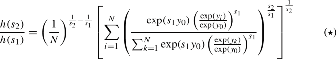
-
3.
For all \(i \in \{1, \dots , N\}\), \(y_i \ge y_0\) and there is \(k \in \{1, \dots , N\}\) with \(y_k = y_0\). These relations are still true when applying the exponential function. However, as \(s_1 < 0\), we have
$$\begin{aligned} \exp (y_i)^{s_1} \le \exp (y_0)^{s_1} \end{aligned}$$and therefore, for all \(i \in \{1, \dots , n\}\), \(a_i \in [0, 1]\) and \(a_k = 1\) for one of them.
-
4.
As \(\frac{s_2}{s_1} > 1\), the auxiliary result 3 can be applied to (\(\star \)), which results in
$$\begin{aligned} \sum _{i = 1}^{N} \left( \frac{\exp (s_1 y_0) \left( \frac{\exp (y_i)}{\exp (y_0)}\right) ^{s_1} }{\sum _{k = 1}^{N} \exp (s_1 y_0) \left( \frac{\exp (y_k)}{\exp (y_0)}\right) ^{s_1} } \right) ^\frac{s_2}{s_1} \ge N^{1 - \frac{s_2}{s_1}} \end{aligned}$$ -
5.
Applying the previous step and remembering \(s_2 < 0\) leads to
$$\begin{aligned} \frac{h(s_2)}{h(s_1)}&= \left( \frac{1}{N}\right) ^{\frac{1}{s_2} - \frac{1}{s_1}} \left[ \sum _{i = 1}^{N} \left( \frac{\exp (s_1 y_0) \left( \frac{\exp (y_i)}{\exp (y_0)}\right) ^{s_1} }{\sum _{k = 1}^{N} \exp (s_1 y_0) \left( \frac{\exp (y_k)}{\exp (y_0)}\right) ^{s_1} } \right) ^\frac{s_2}{s_1} \right] ^{-\frac{1}{|s_2|}} \\&\le \left( \frac{1}{N}\right) ^{\frac{1}{s_2} - \frac{1}{s_1}} \left( \frac{1}{N^{1 - \frac{s_2}{s_1}}}\right) ^\frac{1}{|s_2|} = 1 \end{aligned}$$Hence, \(h(s_2) \le h(s_1)\) for all \(i \in \{1, \dots , N\}\)
-
6.
Finally, again the monotonicity of the logarithm yields
$$\begin{aligned} g^{s_2, t}({\mathbf {x}}) \le g^{s_1, t}({\mathbf {x}}) \end{aligned}$$

Thus, \(\{g^{s, t}\}_{s < 0}\) is monotonically increasing with respect to s.
The statement of the second part can be reversed to \(\{g^{s, t}\}_{-|s| > 0}\) is monotonically decreasing with respect to |s|, which together with the first part is the claim of the lemma. \(\square \)
In the previous proof, the following result from Tsoukalas et al. (2009) is used:
Lemma 3
For all \(b > 1\), \(0 \le a_i \le 1\), \(i \in \{1, \dots , m\}\), we have
Proof of Lemma 2
The proof is done in several steps. To simplify the expressions, for \(i \in \{1, \dots , N\}\) define \(p:= \max _{1\le i \le N} p_i\) and the functions \(g_i({\mathbf {x}}) := \max _{1 \le j\le p_i}g_{ij}({\mathbf {x}})\). Let \({\mathbf {x}} \in {\mathbb {R}}^n\) be arbitrary.
Claim 1: For all \(i \in \{1, \dots , N\}\) and \(t > 0\), the following holds:
Fix \(i \in \{1, \dots , N\}\). By definition, \(g_i({\mathbf {x}}) \ge g_{ij}({\mathbf {x}})\) for all \(j \in \{1, \dots , p_i\}\) with equality for at least one index j. As \(t > 0\) and the exponential function is strictly monotonous and assumes only positive values,
holds. By applying the also monotonous logarithm function, the claim is proven:
The last inequality results from the definition of p.
Claim 2: For all \(i \in \{1, \dots , N\}\), \(t > 0\) and \(s < 0\), the following holds:
The statement follows directly from the first claim under the following operations: First, multiply the inequalities by the negative scalar s. This reverses their order. Afterwards apply the exponential function which keeps the order upright due to its monotonicity.
Claim 3: For all \(s < 0\), the following holds:
By definition, \(g({\mathbf {x}}) \le g_i({\mathbf {x}})\) for all \(i \in \{1, \dots , N\}\). As \(s < 0\), this is equivalent to \(sg({\mathbf {x}}) \ge sg_i({\mathbf {x}})\). Combining this with the fact that
yields
To get the final result, for \(t > 0\) and \(s < 0\), combine claims 2 and 3 to get
Dividing by N and applying the monotonous logarithm yields
Under multiplication with \(s < 0\), the inequalities turn and the claim of the lemma results, when \(g({\mathbf {x}})\) is subtracted :
\(\square \)
The next result is similar to Lemma 1 provides the monotonicity of the shifted entropic smoothing function (11) with respect to the smoothing parameters.
Lemma 4
The family of shifted entropic smoothing functions \(\{{\widetilde{g}}^{s, t}\}_{s, t}\) with \(s < 0\) and \(t > 0\) is monotonically increasing in (|s|, t).
Proof
As it is done for Lemma 1, this proof is splitted in showing the monotonicity behavior for a pair of parameters \(0< t_1 < t_2\) and a pair of parameters \(0> s_1 > s_2\) under the assumption that the other parameter \(s < 0\) or \(t > 0\), respectively, is fixed. The parts of the proof are further segmented into steps.
First, let \(0< t_1 < t_2\) and \( s < 0\) be given. Using the notation that \(p := \max _{1\le i \le N} p_i\), the shifted entropic smoothing function can be restated as follows:
We make the following observations:
-
1.
For \(0< t_1 < t_2\),
$$\begin{aligned} p^{\frac{|s|}{t_1}} \ge p^{\frac{|s|}{t_2}} \end{aligned}$$ -
2.
For all \(i \in \{1, \dots , N\}\), and all \(j \in \{1, \dots , p_i\}\),
$$\begin{aligned} 0 \le \exp \left( t_1 g_{ij}({\mathbf {x}})\right) \le \exp \left( t_2 g_{ij}({\mathbf {x}})\right) \end{aligned}$$ -
3.
For all \(i \in \{1, \dots , N\}\),
$$\begin{aligned}&\sum _{j = 1}^{p_i} \exp \left( t_1 g_{ij}({\mathbf {x}})\right) \le \sum _{j = 1}^{p_i} \exp \left( t_2 g_{ij}({\mathbf {x}})\right) \\&\quad \Longleftrightarrow \left( \sum _{j = 1}^{p_i} \exp \left( t_1 g_{ij}({\mathbf {x}})\right) \right) ^{-1} \ge \left( \sum _{j = 1}^{p_i} \exp \left( t_2 g_{ij}({\mathbf {x}})\right) \right) ^{-1} \end{aligned}$$ -
4.
For all \(i \in \{1, \dots , N\}\),
$$\begin{aligned} \left( \sum _{j = 1}^{p_i} \exp \left( t_1 g_{ij}({\mathbf {x}})\right) \right) ^{-\frac{|s|}{t_1}} \ge \left( \sum _{j = 1}^{p_i} \exp \left( t_2 g_{ij}({\mathbf {x}})\right) \right) ^{-\frac{|s|}{t_2}} \end{aligned}$$ -
5.
$$\begin{aligned} \sum _{i = 1}^ N\left( \sum _{j = 1}^{p_i} \exp \left( t_1 g_{ij}({\mathbf {x}})\right) \right) ^{-\frac{|s|}{t_1}} \ge \sum _{i = 1}^ N \left( \sum _{j = 1}^{p_i} \exp \left( t_2 g_{ij}({\mathbf {x}})\right) \right) ^{-\frac{|s|}{t_2}} \end{aligned}$$
-
6.
Combining 1. and 5., we get
$$\begin{aligned} p^{\frac{|s|}{t_1}} \sum _{i = 1}^ N\left( \sum _{j = 1}^{p_i} \exp \left( t_1 g_{ij}({\mathbf {x}})\right) \right) ^{-\frac{|s|}{t_1}} \ge p^{\frac{|s|}{t_2}} \sum _{i = 1}^ N \left( \sum _{j = 1}^{p_i} \exp \left( t_2 g_{ij}({\mathbf {x}})\right) \right) ^{-\frac{|s|}{t_2}} \end{aligned}$$ -
7.
Applying the monotonous logarithm function does not change the relationship given in 5.
-
8.
Finally, we use \(s < 0\) and get
$$\begin{aligned} \frac{1}{s} \ln&\left( p^{\frac{|s|}{t_1}} \sum _{i = 1}^ N\left( \sum _{j = 1}^{p_i} \exp \left( t_1 g_{ij}({\mathbf {x}})\right) \right) ^{-\frac{|s|}{t_1}} \right) \\&\quad \ge \frac{1}{s} \ln \left( p^{\frac{|s|}{t_2}}\sum _{i = 1}^ N \left( \sum _{j = 1}^{p_i} \exp \left( t_2 g_{ij}({\mathbf {x}})\right) \right) ^{-\frac{|s|}{t_2}} \right) \end{aligned}$$
This shows that the shifted entropic smoothing function is increasing in \(t > 0\).
Second, let \(0> s_1 > s_2\) and \( t > 0\) be given. In this situation, we investigate the parts of another equivalent reformulation of (11):
Here, we make the following observations:
-
1.
For \(0> s_1 > s_2\), and \(i \in \{1, \dots , N\}\),
$$\begin{aligned} \left( \sum _{j = 1}^{p_i} \exp \left( t g_{ij}({\mathbf {x}})\right) \right) ^{\frac{s_1}{t}} \le \left( \sum _{j = 1}^{p_i} \exp \left( t g_{ij}({\mathbf {x}})\right) \right) ^{\frac{s_2}{t}} \end{aligned}$$ -
2.
As a direct result,
$$\begin{aligned} \sum _{i = 1}^N \left( \sum _{j = 1}^{p_i} \exp \left( t g_{ij}({\mathbf {x}})\right) \right) ^{\frac{s_1}{t}} \le \sum _{i = 1}^N \left( \sum _{j = 1}^{p_i} \exp \left( t g_{ij}({\mathbf {x}})\right) \right) ^{\frac{s_2}{t}} \end{aligned}$$ -
3.
Again, the monotinicity of \(\ln \) holds the relation upright, i.e.
$$\begin{aligned}&\ln \left( \sum _{i = 1}^N \left( \sum _{j = 1}^{p_i} \exp \left( t g_{ij}({\mathbf {x}})\right) \right) ^{\frac{s_1}{t}} \right) \le \ln \left( \sum _{i = 1}^N \left( \sum _{j = 1}^{p_i} \exp \left( t g_{ij}({\mathbf {x}})\right) \right) ^{\frac{s_2}{t}} \right) \\&\quad \Longleftrightarrow -\ln \left( \sum _{i = 1}^N \left( \sum _{j = 1}^{p_i} \exp \left( t g_{ij}({\mathbf {x}})\right) \right) ^{\frac{s_1}{t}} \right) \ge -\ln \left( \sum _{i = 1}^N \left( \sum _{j = 1}^{p_i} \exp \left( t g_{ij}({\mathbf {x}})\right) \right) ^{\frac{s_2}{t}} \right) \end{aligned}$$ -
4.
Finally, we get from \(|s_1| < |s_2|\),
$$\begin{aligned} -\frac{1}{|s_1|}\ln \left( \sum _{i = 1}^N \left( \sum _{j = 1}^{p_i} \exp \left( t g_{ij}({\mathbf {x}})\right) \right) ^{\frac{s_1}{t}} \right) \ge -\frac{1}{|s_2|}\ln \left( \sum _{i = 1}^N \left( \sum _{j = 1}^{p_i} \exp \left( t g_{ij}({\mathbf {x}})\right) \right) ^{\frac{s_2}{t}} \right) \end{aligned}$$
This shows that the shifted entropic smoothing function is monotonous decreasing as \(0 > s \rightarrow -\infty \).
Bringing both parts of the proof together, shows the claim. \(\square \)
Numerical handling of the double and shifted entropic smoothing
In order to stabilize the numerical evaluations of the exponential functions in the double and shifted entropic smoothing functions, we use the trick of "adding zeros" as follows: Let \(z_i \in {\mathbb {R}}\) for \(1\le i \le n\), \(n \in {\mathbb {N}}\) and \(c \in {\mathbb {R}}\) be real numbers. Then the following terms are equal:
We apply this "addition of zero" twice to the double entropic smoothing function used in our numerical experiments: First, we reduce the arguments of the inner exponentials by the constants
Then, we use the minimum of the reduced inner terms as reduction constant for the outer N exponentials:
To sum up, we get the following numerically stable double entropic smoothing function (9):
Rights and permissions
Open Access This article is licensed under a Creative Commons Attribution 4.0 International License, which permits use, sharing, adaptation, distribution and reproduction in any medium or format, as long as you give appropriate credit to the original author(s) and the source, provide a link to the Creative Commons licence, and indicate if changes were made. The images or other third party material in this article are included in the article’s Creative Commons licence, unless indicated otherwise in a credit line to the material. If material is not included in the article’s Creative Commons licence and your intended use is not permitted by statutory regulation or exceeds the permitted use, you will need to obtain permission directly from the copyright holder. To view a copy of this licence, visit http://creativecommons.org/licenses/by/4.0/.
About this article

Cite this article
Krieg, H., Seidel, T., Schwientek, J. et al. Solving continuous set covering problems by means of semi-infinite optimization. Math Meth Oper Res 96, 39–82 (2022). https://doi.org/10.1007/s00186-022-00776-y
Received:
Revised:
Accepted:
Published:
Issue Date:
DOI: https://doi.org/10.1007/s00186-022-00776-y