Spectroscopy of planetary atmospheres in our Galaxy

Abstract

About 20 years after the discovery of the first extrasolar planet, the number of planets known has grown by three orders of magnitude, and continues to increase at neck breaking pace. For most of these planets we have little information, except for the fact that they exist and possess an address in our Galaxy. For about one third of them, we know how much they weigh, their size and their orbital parameters. For less than 20, we start to have some clues about their atmospheric temperature and composition. How do we make progress from here?

We are still far from the completion of a hypothetical Hertzsprung–Russell diagram for planets comparable to what we have for stars, and today we do not even know whether such classification will ever be possible or even meaningful for planetary objects. But one thing is clear: planetary parameters such as mass, radius and temperature alone do not explain the diversity revealed by current observations. The chemical composition of these planets is needed to trace back their formation history and evolution, as happened for the planets in our Solar System. As in situ measurements are and will remain off-limits for exoplanets, to study their chemical composition we will have to rely on remote sensing spectroscopic observations of their gaseous envelopes.

In this paper, we critically review the key achievements accomplished in the study of exoplanet atmospheres in the past ten years. We discuss possible hurdles and the way to overcome those. Finally, we review the prospects for the future. The knowledge and the experience gained with the planets in our solar system will guide our journey among those faraway worlds.

1 Overview

Before 1995, the planets known were nine, i.e. the planets orbiting our favourite star, the Sun, plus Pluto. Eighteen years later, we have “lost” Pluto but, on the other hand, we have gained a thousand planets planets in orbit around other stars and this number appears far from being final. The current statistical estimates seem to indicate that, on average, every star in our Galaxy hosts at least one planetary companion (Cassan et al. 2012). Given that the number of stars in the Milky Way is estimated to be ∼10¹¹, planetary scientists are expected to be kept busy in the next years!

While the number of planets discovered is still far from the hundreds of billions mentioned above, the NASA Kepler mission alone has announced thousands of planetary candidates, which await confirmation (Borucki et al. 2011, Batalha et al. 2013). The European Space Agency GAIA mission is expected to deliver several thousands new planets via the astrometric technique (Casertano et al. 2008; Sozzetti 2010). The NASA TESS mission (Ricker et al. 2010) is predicted to discover thousands transiting exoplanet candidates which are Earth-sized or larger. Are those numbers large enough to provide a meaningful classification of planets as we do with stars?

Astrophysics faced a similar situation with the classification of stars in the 20th century. The striking observational phenomenon that the stellar brightness correlates with its perceived colour was first noted by Russell (1910) and Hertzsprung (1912) and allowed to link observations to a deep understanding of the stellar interior and of the nuclear power source (Eddington 1924; Bethe 1939). It was soon realised that, at first approximation, a star’s structure was uniquely determined by its mass, initial chemical composition and age (i.e. the so-called Vogt–Russel theorem), and that, as a consequence, in a given phase of star’s lifespan (main sequence, giant branch, etc.) key parameters such as temperature, mass, etc., are well correlated. This behaviour is a powerful observational tool that permits to derive, even if with some caveats, a wide range of stellar parameters from a few basic observables.

Conversely, the knowledge of the mass may provide very little information about a planet, namely if it is a gas giant, an icy giant or a rocky one, and sometimes the last two categories cannot be distinguished from each other. For a planetary body, mass, radius, temperature and chemical composition are often loosely correlated parameters, and cannot be disentangled from the initial conditions, history and interaction with the mother star. Even within the frontiers of our Solar System, there is a large variety of cases, and one can hardly find two bodies with similar characteristics. One would expect the complexity to increase when we cross the Kuiper belt boundaries and, from the little we know, this seems indeed to be the case. At the same time, only by putting the Sun’s planets and environment in a broader context, we can interpret correctly why is the Solar System as it is today.

The discovery of 51 Peg b by Mayor and Queloz (1995) represented a turning point in the history of planets. This was not just the first exoplanet detected around a main sequence star. The very existence of 51 Peg b was a true challenge to the “nebular theory” of planetary formation, according to which gas giants need to form in the peripheral areas of the disc where most of the gas, ice and dust are located. To justify 51 Peg b and other similar objects currently known as “hot-Jupiters”, migration mechanisms were invoked. To justify why Jupiter and Saturn did not migrate in, as many of their gaseous siblings, the “Nice” model was conceived (Gomes et al. 2005; Tsiganis et al. 2005; Morbidelli et al. 2005; Walsh et al. 2011). All of a sudden the Solar System had to be explained as an exception rather than being the standard model: this was a paradigm shift that challenged irreversibly our “heliocentric” view of the Universe.

During the past years, planets have been found around every type of stars from A to M, including pulsars and binaries. Being the leftover of the stellar formation process, planets appear to be rather ubiquitous, and in reality, the presence of a host star is not always a mandatory circumstance (Zapatero-Osorio et al. 2000; Sumi et al. 2011).

Another prejudice that fell, was the idea that, based on some selection rules suggested by the orbital shapes of the Sun’s planets, all planetary orbits had to be nearly circular. Today we appreciate that more than 60 % of the exoplanets known move on elliptical orbits, and in some cases the eccentricity reaches quite extreme values (Fig. 1). If the orbit is very eccentric, the insolation changes dramatically through the orbital period (Sertorio and Tinetti 2002; Williams and Pollard 2002; Iro and Deming 2010; Laughlin et al. 2009; Dobrovolskis 2013). The axial tilt and the ratio between the rotation and orbital periods also play a pivotal role in the spatial-temporal distribution of the stellar irradiation on the planet (Williams and Kasting 1997; Sertorio and Tinetti 2002). In our Solar System, most of the planets have an axial tilt which is less than 27 degrees, with the exception of Uranus, whose rotation axis is approximately parallel with the ecliptic plane. Up to date, it has not been possible to constrain the obliquity of an exoplanet. For the Sun’s planets, rotation periods vary from a fraction of a day for gas and icy giants, to about one day for the Earth and Mars. In the case of Venus and Mercury, their rotation period is very similar to their annual period. For planets orbiting very close to their stellar companion, in fact, gravitational interaction with their host star may result in the orbit circularisation and the synchronisation of the rotation and revolution periods (Sect. 2).

Fig. 1

Orbital eccentricity versus semi-major axis for known exoplanets (Schneider et al. 2013)

The measurement of the planetary radius through transit observations (Charbonneau et al. 2000; Henry et al. 2000) combined with the measurement of the mass with radial velocity, allowed for the very first estimates of the planetary bulk densities. This information is available today for almost 400 planets. We show in Fig. 2 a mass-radius diagram from Winn et al. (2011). The additional information provided by the planetary radius has stimulated very interesting theoretical work and debates, but it is not sufficient to clarify the “big picture”. From Fig. 2, we appreciate that even the giant gaseous planets have a rather spread-out distribution of densities, hinting at a variety of internal structures/core compositions (e.g. Guillot et al. 2005; Fortney et al. 2007). Objects lighter than ten Earth masses are even more enigmatic, as they can be explained in different ways (Valencia et al. 2006, 2007; Sotin et al. 2007; Seager et al. 2007; Adams et al. 2008; Grasset et al. 2009).

Fig. 2

Masses and radii of transiting exoplanets (fig. from Winn et al. 2011). Coloured lines show mass-radius relations for a variety of internal compositions

Knowing the star-planet distance and the type of the stellar companion, we can infer the planetary equilibrium temperature. This information can be used as a first guess to predict the most probable chemical composition of the planetary atmosphere (Sect. 2). When we consider gaseous planets, which we know being composed mainly by molecular hydrogen, this description could be a good approximation to portray a static, thermochemical equilibrium case. Conversely, we would completely ignore any perturbation caused by the variety of initial conditions and later events. We would also disregard the impact of photochemistry and transport-induced quenching of disequilibrium species. When it comes to terrestrial-type planets, the spectrum of possibilities is indeed much larger compared to the gaseous objects: it is very difficult to guess a priori what the main atmospheric component should be, if any.

Constraints to the theoretical predictions need to come from the observations, as happened for the planets in our own Solar System. The difficulty here is that we cannot conceive in situ measurements in a foreseeable future, so our knowledge has to rely on remote sensing observations. At present, two techniques can be used to sound the atmospheres of exoplanets: the transit method and direct imaging. These are very complementary techniques, as they can probe different categories of planets. Let us focus first on the gaseous ones.

The transit technique may provide insight about planets which were formed in the outer regions of their planetary disc and then migrated in (Fig. 3). Transit spectroscopy is, therefore, an excellent diagnostic to understand objects which have experienced a rather dramatic history, and probably substantial modifications, given the extreme conditions in which they are and have been exposed to. We do not know today whether or not transiting gaseous planets have maintained any chemical trace of their formation and migration history. If not, then it should be relatively easy to classify such objects according to the temperature and the type of stellar companion, as those should be the key ingredients to model the current atmospheric composition. Needless to say, in this case it would be extremely difficult to reconstruct the formation and evolution history of these planets, as no chemical memory of the past would have been preserved. By contrast, if the initial conditions play an important role in the current structure and composition of these planets, then a variety of cases should be expected, and an accurate classification would be rather difficult. Although scientists like rigorous classifications, as they allow for a simplified description of the reality through a few parameters, the second hypothesis is certainly more intriguing and probably more realistic.

Fig. 3

Key questions that can be addressed by transit spectroscopy

In parallel with transit studies, in the next decade, direct imaging is expected to provide insight about hot, young planets at large separations from their parent star—i.e. gaseous planets newly formed in the outer regions of their planetary disc and not (yet?) migrated in—or planets formed closer in and then kicked out through dynamical interactions with the other planets in the disc. The first spectrum of a hot, giant planet, at a projected separation of 38 AU from its host star, was observed with the ESO Very Large Telescope (VLT)/NACO by Janson et al. (2010). Photometric data in the NIR were obtained for a couple of similar planets (Currie et al. 2011; Barman et al. 2011). Spectroscopy in the wavelength range of YJHK-band will start soon with dedicated instruments on VLT (SPHERE) and Gemini (GPI). By comparing the chemical composition of these young gaseous objects to the composition of their migrated siblings probed through transit, we should be able to understand better the role played by migration and by extreme irradiation on gaseous planets formation and evolution. Further into the future, this technique should also provide information about “old”—and therefore cold—gaseous planets at large separation, i.e. planets more similar to Jupiter and Saturn, allowing for a direct comparison with the Solar System’s gas giants.

The story for smaller, terrestrial-type planets could be radically different: several scenarios might occur (Fig. 3). To start with, these objects could have been formed in situ, or have moved from their original location because of dynamical interaction with other bodies (Raymond et al. 2009), or they could be remnant cores of more massive gaseous objects migrated in Grasset (2013).

Having lower masses, their atmospheres may have evolved quite dramatically from their initial composition: lighter molecules, like hydrogen, can escape more readily (Sect. 3.2). This certainly happened to the terrestrial planets in our Solar System: in Venus’ and Mars’ atmospheres the D/H ratio is between 5 and 200 times the Solar ratio, suggesting water on the surface was lost through time (Owen et al. 1988; Encrenaz 2009). Impacts with other bodies, such as asteroids or comets, or volcanic activity might also significantly alter the composition of the primordial atmosphere, not to mention life, which on Earth is responsible e.g. for the production of molecular oxygen, accounting for 21 % of the overall atmospheric volume (Lovelock 1975; Rye and Holland 1998).

At its dawn, the field of exoplanets has been predominantly driven by the search for extraterrestrial life and other habitable worlds. This search was heavily biased towards a geocentric concept of habitable planet: such a planet had to weigh like the Earth, had to orbit a star similar to the Sun, on a quasi-circular orbit at the right distance to allow for the presence of liquid water, etc. (Sect. 6). To get to the “Earth-twin”, no experiment appeared to be too challenging or expensive (Bracewell 1978; Angel et al. 1986; Léger et al. 1996).

The discovery of the super-Earths, planets with masses between the Earth mass and ten Earth masses, has shaken this pre-Galilean view of how a habitable world should or should not be. Because of their larger size compared to our own planet, the super-Earths have opened new perspectives in terms of observability. Transit spectroscopy is the ideal technique to probe temperate planets around M-dwarfs. These are by far the most common type of stars in our Galaxy, albeit much smaller, dimmer and cooler than stars like our sun: if the host star is bright enough, these objects are within reach the current or the near-term future facilities (Bean et al. 2010; Berta et al. 2012). For temperate planets around earlier-type stars, direct imaging will be a more appropriate technique as transit observations would be rather impractical in these cases. The hunt for exo-moons as other possible abodes of life is now one of the hottest subject (Williams et al. 1997; Sartoretti and Schneider 1999; Kipping 2009a, 2009b). While the race to find the very first one with Kepler (Kipping et al. 2009) or other techniques (Han 2008; Lewis et al. 2008; Simon et al. 2009) has become rather fierce, the new ESA Jupiter Icy Moon Explorer (JUICE) mission will provide new insight about Jupiter’s environment and its impact on the Galilean moons (Dougherty et al. 2012).

In the following sections, we give a brief overview of the transit method to sound exoplanet atmospheres and we report key achievements accomplished in the last ten years in this exciting new field (Sect. 2). While photometric and spectroscopic observations of gaseous planets with Spitzer, Hubble and ground-based observatories have provided the very first detections of ionic, atomic and molecular species in some of those exotic atmospheres, the data available are still too sparse to provide a consistent interpretation, or any meaningful classification of the planets analysed. More and better-quality data are needed for this purpose. Atmospheric models of exoplanets, inferred from their equilibrium temperature and associated with different mechanisms are discussed in Sects. 3 and 4. In Sect. 5, infrared spectra of exoplanets are presented, with a discussion of the need for better spectroscopic data. In the next decade, a combination of new, larger telescopes and improved instrumentation, together with dedicated space missions currently under study, should do the trick (Sect. 7).

And what will be the next steps to take once we have understood everything we need to know about planets in our own Galaxy? For planets in galaxies at redshift z∼0, one would expect the very same conclusions should be drawn, as the Universe is homogeneous and isotropic on a macroscopic scale. The question becomes interesting for planets in Galaxies at high redshift, which is equivalent to digging in our past. In those galaxies, star formation processes and stellar metallicity might be radically different from the current situation in the Milky Way (e.g. Trenti et al. 2012 and ref. therein). As explained in Sect. 4, stellar metallicity is expected to have an important impact on planetary formation.

And what about the future? If the Universe is expanding at an accelerating pace (Riess et al. 1998; Perlmutter et al. 1999; Komatsu et al. 2011), then we should probably expect a cold and lonely end (Dyson 1979). But that is another story, and maybe we should leave this one to cosmologists.

2 Transit spectroscopy: what can it tell us?

The transit phenomenon takes place when a celestial body, as seen from Earth, crosses the path of a more distant object with an angular diameter larger than its own. If the distant body has a smaller diameter, the event is called an occultation. The most popular event of this kind is the solar eclipse by the Moon, where both objects have typically the same angular diameter. In the solar system, transits of Venus and Mercury in front of the Sun are occasionally observed, but occultations of other solar-system objects in front of stars are also known to happen. Planetary transits have been observed since perhaps the dawn of civilisation (Avicenna, ∼1000 A.D.). Despite the Seven Years’ War, the transit of Venus in 1761 marked the first scientific project undertaken on an international scale.

The same phenomenon can occur in the case of exoplanets whose orbits are aligned so they cross the surface of their mother star when viewed from Earth. When the planet passes in front of the star, the event is called a primary (or direct) transit; when it passes behind the star, it is called a secondary (or indirect) transit or an eclipse or, more properly, an occultation. In what follows, we call the events primary transit and secondary eclipse as these terms are most commonly used in the literature. In both cases, the information on the exoplanet’s atmosphere is retrieved from the flux difference of the star + planet system before, during and between the transit. Such observations are at the limit of detectability in terms of sensitivity, as the planet to star flux contrast, in the best cases—hot Jupiters—is about 10⁻⁶ in the visible range and a few 10⁻³ in the mid-infrared range (10 μm).

An important parameter to consider for understanding the atmospheric behaviour of transiting exoplanets is their rotation. For solar-type stars, planets located within 0.05 AU from their host star are predicted to be tidally locked, i.e. they always show the same face to the star. This effect is due to gravitational interaction which results in the orbit circularisation and the synchronisation of the rotation and revolution periods. The critical distance for tidal lock is about 0.5 AU for a solar-type star, and is proportional to [M ^∗]^1/3 for a star of mass M ^∗ (Kasting et al. 1993). For M-type stars of 0.1 and 0.01 solar mass, planets are thus expected to be tidally locked within a distance of 0.2 AU and 0.08 AU, respectively (Forget and Wordsworth 2010). As the stellar flux is always concentrated on the same hemisphere of the planet, strong atmospheric circulation should take place between the dayside and the nightside (see e.g. Cho et al. 2003, 2008; Cooper and Showman 2005, 2006; Iro et al. 2005; Rauscher et al. 2007, 2008a, 2008b; Thrastarson and Cho 2010). This circulation pattern can be studied by monitoring the planetary phase curve (see Sect. 2.3).

2.1 Primary transits

2.1.1 Geometry of a primary transit

When a planet passes in front of its host star, the star flux is reduced by a few of percent, corresponding to the planet/star surface ratio. The planetary radius can be inferred from this measurement. If atomic or molecular species are present in the exoplanet’s atmosphere, the inferred radius is larger at some specific wavelengths (absorption) corresponding to the spectral signatures of these species (Seager and Sasselov 2000; Brown 2001, Tinetti et al. 2007b).

At zero-order approximation, the area of planetary atmospheres observed in transmission is an annulus around the planet with a radial height of a few scale heights (usually four or five in the infrared). The scale height H is equal to kT/μg, where k is the Boltzmann constant, T the temperature, μ the mean molecular weight of the atmosphere and g the planet’s gravity. The amplitude of the absorption can be approximated as

$$ A \sim 5 \cdot [2R_{p}H/R^{*2}] $$

(1)

where R _p and R ^∗ are the radii of the planet and the star, respectively. The signature is especially strong for hot planets, light atmospheres and low gravity objects. “Hot Jupiters” are therefore privileged targets for primary transits.

Primary transits probe the exoplanet’s atmosphere at the terminator, at both morning and evening sides. In the case of tidally locked planets, this observation is of special interest for probing sub-stellar to anti-stellar winds, as observed, on a much lower scale, in the case of the Venus mesosphere (Goldstein et al. 1991). Primary transit spectroscopy has some advantages in the identification of the atmospheric constituents, as all species are observed in absorption along the line of sight. The information is retrieved on their column densities, i.e. on their partial pressures at a given atmospheric level corresponding to an optical depth of unity. By contrast, absolute measurements of the molecular abundances are not always obtainable. These considerations cannot be explained by the approximation (1), and we need to show the complete calculations. We use here the notation adopted by Tinetti et al. (2012a, 2012b), see also Seager and Sasselov (2000), Brown (2001).

According to Beer–Bouguer–Lambert’s law, we have

$$ I(\lambda,z )=I_0e^{-\tau(\lambda ,z)}; \qquad \tau(\lambda,z)=\sum_i\tau_i(\lambda,z) $$

(2)

where:

I ₀ :

= stellar radiation intensity

I :

= stellar radiation intensity filtered through the planetary atmosphere

λ :

= wavelength

z :

= altitude above R _p

τ :

= optical path

i :

= absorber

To convert the altitude (observable) to pressure (thermodynamic variable) we use the hydrostatic equilibrium approximation and the ideal gas law for a gas of N particles and volume V, which are reasonable approximations below the homopause.¹ We have

$$ \frac{p}{\rho}=kT;\qquad \mathrm{d}p=\mu\rho g\,\mathrm{d}z;\qquad \rho=\frac{N}{V} $$

(3)

The quantum interaction between the photons and the atmospheric absorbers is accounted for in the calculation of the optical path (e.g. Goody and Yung 1989):

$$ \tau_i(\lambda ,z)=2\int_{0}^{\ell(z)}\rho\bigl(z'\bigr)\chi_i\bigl(z'\bigr) \sigma_i(\lambda ,T)\,\mathrm{d }\ell; $$

(4)

In (4) σ _i and χ _i are the absorption coefficient and the mixing ratio for the ith absorber. The path traversed by stellar photons, ℓ, can be easily obtained through geometrical calculations (see Fig. 4):

$$\begin{aligned} \mathrm {d}\ell =&\sqrt{\bigl(R_p+z'+\mathrm {d}z'\bigr)^2-(R_p+z)^2} - \sqrt{\bigl(R_p+z'\bigr)^2-(R_p+z)^2}\\ \ell(z) =&\int \mathrm {d}\ell=\sqrt{(R_p+z_{\max})^2-(R_p+z)^2} \end{aligned}$$

Finally, the transit depth as a function of wavelength is given by

$$ \begin{aligned} k(\lambda )&=\displaystyle\frac{R_p^2 +2\int_0^{z_{\max}}(R_p+z)(1-e^{-\tau(z,\lambda )})\,\mathrm {d}z}{R_*^2} \\ A(\lambda) &=\displaystyle \frac{2\int_0^{z_{\max}}(R_p+z)(1-e^{-\tau(z,\lambda )})\,\mathrm {d}z}{R_*^2} \end{aligned} $$

(5)

Equation (5) has a unique solution provided we know R _p accurately. R _p is the planetary radius at which the planet becomes opaque at all λ. For a terrestrial planet, R _p usually coincides with the radius at the surface. In contrast, for a gaseous planet, R _p may correspond to a pressure p ₀∼1–10 bar, depending on the transparency of the atmosphere.

Fig. 4

Geometry of transit spectroscopy: the photons from the star are filtered through the atmosphere of the planet

From Eqs. (4) and (5) we can estimate the molecular/atomic abundances, χ _i , only if the atmosphere is transparent in some spectral bands, so that we can use those intervals to measure R _p . For gaseous planets, the level of the continuum in the IR is given by H₂–H₂ (Borysow et al. 2001) if there are no clouds. If molecules such as water vapour are present, it is more difficult to estimate R _p : H₂O absorbs continuously and strongly in all the IR, leaving out just the UV–VIS and part of the NIR. These spectral intervals can be used to estimate R _p only if no clouds are present. Given that hot-Jupiters’ spectra are dominated by water vapour absorption, this explains the origin of the degeneracy of molecular abundances retrieved from observations.

2.1.2 Primary transit observations

The upper atmosphere of an exoplanet can be effectively probed by transit technique and transmission spectroscopy (Coustenis et al. 1997). Observations from space, with HST/STIS-COS, and from the ground, unveiled a population of ions and radicals wrapping the planet like an envelope and partially occulting the star. These observations are suggestive of escape processes: Jeans escape or hydrodynamical mechanisms (Vidal-Madjar et al. 2003, 2004; Ben-Jaffel 2007, 2008; Ben-Jaffel and Hosseini 2010; Linsky et al. 2010; Lecavelier des Etangs et al. 2010, 2012; Fossati et al. 2010; Jensen et al. 2012). We show in Fig. 5 the results published by Linsky et al. (2010) for C II, obtained with Hubble-COS.

Fig. 5

Detection of C II in the exosphere of HD209458b with Hubble-COS (Linsky et al. 2010)

After the discovery of Na in the atmosphere of HD209458b (Charbonneau et al. 2002), repeated measurements of alkali metals on other planets have been reported in the literature, from space and the ground (e.g. sodium: Redfield et al. 2008; Snellen et al. 2008; Wood et al. 2011; potassium: Colon et al. 2010; Sing et al. 2011a). For some of these planets, the authors estimate the abundances of the alkali metals to be greatly depleted relative to solar and attribute this effect to the presence of clouds or to photo-ionisation. An interesting, alternative explanation was proposed by Atreya et al. (2003), who suggested that, instead of being primordial, the observed alkali metals may be largely of non-planetary origin, i.e. from debris, meteorites and comets.

Hazes or clouds of unknown composition may affect the transparency of some of the observed atmospheres in the visible spectral range (e.g. Knutson et al. 2007; Barman 2007; Pont et al. 2008; Sing et al. 2011b). The hot-Jupiters XO-1b and XO-2b (Tinetti et al. 2010; Crouzet et al. 2012), WASP-12b (Swain et al. 2012), HD209458b (Deming et al. 2013) and HD189733b (Danielski et al. 2012) show instead distinctive molecular features in the NIR spectral region (Fig. 6).

Fig. 6

Collection of IR transit data recorded and interpreted by multiple teams, see discussion in Sect. 2.1.2. Top figures: NIR transit spectra for HD189733b observed with Hubble-NICMOS (left, Swain et al. 2008, see also Waldmann et al. 2013) and from the ground (right, Danielski et al. 2012). Centre: best solution retrieved by Madhusudhan and Seager (2009). Second row: differential photometric data and spectrum for HD209458b. Left and centre: data observed with Spitzer IRAC and MIPS and interpretations (Beaulieu et al. 2010; Burrows et al. 2010). Right: transit spectrum observed with Hubble WFC3 (Deming et al. 2013). Third row: NIR transit spectra recorded with NICMOS for XO1-b (left: Tinetti et al. 2010) and XO2-b (fourth row, Crouzet et al. 2012) and interpretations. Bottom figure: available data from space and the ground and interpretation for GJ 1214b (Berta et al. 2012, see also Bean et al. 2010)

The infrared range offers the possibility of probing the neutral atmospheres of the exoplanets. Observations have been performed from space with Spitzer/IRAC-IRS-MIPS and with the Hubble Space Telescope/NICMOS-WFC3, and from the ground (VLT, IRTF, Keck), see Fig. 6. In the IR the spectral features are more intense and broader than in the visible (Tinetti et al. 2007b), hence easier to detect.

On a large scale, the transmission spectra of hot-Jupiters seem to be dominated by the signature of water vapour (Barman 2007, 2008; Beaulieu et al. 2010; Burrows et al. 2007, 2008, 2010; Charbonneau et al. 2008; Grillmair et al. 2008; Knutson et al. 2008; Madhusudhan and Seager (2009); Tinetti et al. 2007a, 2007b, 2010), whereas warm Neptunes, such as GJ 436b and GJ 3470b, are expected to be methane-rich (Beaulieu et al. 2011; Fukui et al. 2013). The analysis of GJ 436b cannot be considered conclusive, though, given the activity of the star (Knutson et al. 2011) and the lack of spectroscopic data: only photometric data, often recorded at different times, are available for this target. The presence of methane is predicted by photochemical models (Moses et al. 2011; Line et al. 2011), but would need further spectroscopic confirmation on a larger sample of targets. The HST/NICMOS transit observations of the planet HD189733b (Swain et al. 2008) led to the identification of H₂O and CH₄ in the atmosphere of that planet (see also Waldmann et al. 2013 and Madhusudhan and Seager 2009). CO is a tricky molecule to detect from space, as the spectral resolution obtainable is not sufficient to distinguish it from CH₄ or CO₂. The method pioneered by Snellen et al. (2010) using the VLT-CRIRES instrument, allowed for the first robust detection of CO in the atmospheres of HD209458b and HD189733b (De Kok et al. 2013). The method can be used also for non-transiting planets, as shown by Brogi et al. (2012) on τ Bootis b, opening a new field of applications of this powerful technique.

The ∼6 Earth mass, warm planet GJ 1214b (Charbonneau et al. 2009) has been the first super-Earth to be probed spectroscopically (Bean et al. 2010). The VLT observations were followed by other space and ground data (Bean et al. 2011; Croll et al. 2011; Crossfield et al. 2011; Désert et al. 2011; Berta et al. 2012) which are suggestive of an atmosphere heavier than pure molecular hydrogen, but additional observations are needed to confirm its composition (see Fig. 6).

In the past, parametric models have extensively been used by several teams to remove the instrument’s systematic effects (e.g. Agol et al. 2010; Beaulieu et al. 2008, 2010, 2011; Brown 2001; Burke et al. 2010; Charbonneau et al. 2005, 2008; Deming et al. 2013; Désert et al. 2011; Grillmair et al. 2008; Knutson et al. 2007; Machalek et al. 2009; Pont et al. 2008; Sing et al. 2011a; Stevenson et al. 2010; Swain et al. 2008, 2009b). Parametric models approximate systematic noise via the use of auxiliary information of the instrument, the so-called optical state vectors, which often include the positional drifts of the star on the detector, the focus and the detector temperature changes, the positional angles of the telescope on the sky etc. In the case of dedicated missions, such as Kepler (Jenkins et al. 2010), the instrument response functions are well characterised in advance and conceived to reach the required 10⁻⁴ to 10⁻⁵ photometric precision. For general purpose instruments, not calibrated to reach this required precision, poorly sampled optical state vectors or a missing parameterisation of the instrument often become critical issues. The way forward is to adopt new and independent data analysis techniques to break the noise-result degeneracy more efficiently and recover the original results (Waldmann 2012, 2013; Waldmann et al. 2013). Statistical techniques used in cosmology and communication science to optimise the extraction of a weak signal from a noisy background find more and more applicability in the analysis of exoplanetary signals (e.g. Carter and Winn 2009; Gregory 2011; Feroz et al. 2011; Gibson et al. 2012).

2.2 Secondary eclipses

A direct measurement of the planet’s emission/reflection can be obtained through the observation of the planetary eclipse, by recording the difference between the combined star + planet signal, measured just before and after the eclipse, and the stellar flux alone, measured during the eclipse. In contrast with the primary transit observations, the dayside of the planet is observed, which makes both methods fully complementary.

As discussed in Sect. 5.1, infrared spectra—typically above 1 μm—are dominated by thermal emission and the observed spectra strongly depend on the atmospheric thermal structure. If a stratosphere is present, molecular signatures can appear either in emission or in absorption, depending on their formation region, above or below the tropopause (see, e.g. Encrenaz et al. 2004; Sect. 5.1); the interpretation of the spectrum is thus less obvious, as it requires the simultaneous retrieval of the vertical distribution of the temperature.

Observations provide measurements of the flux emitted and/or reflected by the planet in units of the stellar flux (Charbonneau et al. 2005; Deming et al. 2005). The planet/star flux ratio η(λ) is defined as

$$ \eta(\lambda) = \bigl(R_{p}/R^{*}\bigr)^{2} {F}_{p}(\lambda)/{F}^{*} (\lambda) $$

(6)

The stellar and planetary spectra can be modelled by radiative-transfer calculations, accounting for scattering processes, ionic, atomic and molecular opacities (see e.g. Chandrasekhar 1960; Goody and Yung 1989; Liou 2002)

At zero-order approximation, the emitted component of the planetary contribution can be estimated by blackbody curves at the stellar and planetary temperatures (T ^∗ and T _p ):

$$ \eta(\lambda) = \bigl(R_{p}/R^{*}\bigr)^{2} B_{p}(\lambda,T_{p})/B^{*}(\lambda,T_{p}) $$

(7)

For the reflected component, at zero-order one can write

$$ \eta(\lambda) = \bigl(R_{p}/R^{*}\bigr)^{2} A \zeta \bigl(R^{*2}/D^{2} \bigr) F^{*}(\lambda)/F^{*} (\lambda) = (R_{p}/D)^{2} A \zeta $$

(8)

where A is the planetary albedo ζ is the observed fraction of the planet illuminated and D the semi-major axis.

Combining near-infrared (NIR) with mid-infrared (MIR) eclipse spectra from space and ground measurements, a consensus has been reached that the absorptions due to H₂O, CH₄, CO and CO₂ explain most of the features present in the hot-Jupiters analysed. In Fig. 7a, we show the photometric and spectroscopic data relative to the planet HD189733b, collected by multiple teams using Spitzer IRAC/IRS/MIPS (Charbonneau et al. 2008; Grillmair et al. 2008; Deming et al. 2006) and Hubble NICMOS (Swain et al. 2009a, 2009b), and their interpretations (Swain et al. 2009a, 2009b; Madhusudhan and Seager 2009; Lee et al. 2012; Line et al. 2012). In Fig. 7b, we show the photometric and spectroscopic data relative to the planet HD209458b collected by different teams using, Spitzer IRAC/IRS/MIPS (Knutson et al. 2007; Swain et al. 2008; Deming et al. 2005) and Hubble NICMOS (Swain et al. 2009b), and the related interpretations (Burrows et al. 2007; Swain et al. 2009b; Madhusudhan and Seager 2009). While the different radiative-transfer models and spectral retrieval schemes adopted indicate the same atmospheric composition, there is no agreement on the abundances retrieved. This is only in part due to the degeneracy embedded in the observations,—which are often sparse and with large uncertainties—and in the well-known difficulty associated with emission spectroscopy in retrieving simultaneously the thermal profile and the molecular abundances. The different spectroscopic line lists adopted by the different teams play an important role (see Sects. 5.3.2 and 5.3.5).

Fig. 7a

Available data for HD189733b observed by multiple teams using secondary eclipse method and retrieved solutions. The data were recorded with Spitzer IRAC/IRS/MIPS (Charbonneau et al. 2008; Grillmair et al. 2008; Deming et al. 2006) and Hubble NICMOS (Swain et al. 2009a, 2009b). The spectral simulations and data interpretations, were performed by different teams, using radiative-transfer models and spectral retrieval methods. All the teams conclude the best fit is obtainable with a combination of H₂O, CH₄, CO and CO₂. Top left: best fit by Tinetti and Griffith (Swain et al. 2009a; Tinetti and Griffith 2010). Top right: best solutions retrieved by Madhusudhan and Seager (2009). Bottom left: best fit by Lee et al. (2012). Bottom right: best solutions retrieved by Line et al. (2012)

Fig. 7b

Available data for HD209458b observed by multiple teams using secondary eclipse method and retrieved solutions. The data were recorded with Spitzer IRAC/IRS/MIPS (Knutson et al. 2007; Swain et al. 2008; Deming et al. 2005) and Hubble NICMOS (Swain et al. 2009b). The spectral simulations and data interpretations, were performed by different teams, using radiative-transfer models and spectral retrieval methods. All the teams agree that water vapour and the presence of a stratosphere are a good baseline to fit the data. Models including data from NICMOS, conclude the best fit is obtainable with a combination of H₂O, CH₄, CO and CO₂. Top left: best fit by Burrows et al. (2007). Top right: best solutions retrieved by Griffith and Tinetti (Griffith and Tinetti 2010; Swain et al. 2009b). Bottom: best solutions retrieved by Madhusudhan and Seager (2009)

An unexpected result from the ground is the detection of a methane emission at 3.3 μm in HD189733b, attributed to non-LTE mechanisms (Swain et al. 2010; Waldmann et al. 2012), which opens new perspectives for future ground-based transit observations.

2.3 Planet phase-variations

In addition to transit and eclipse observations, monitoring the flux of the star+planet system over the orbital period allows to retrieve information on the planet emission at different phase angles. Such observations have to be performed from space, as they typically expand over a time interval of more than a day.

In the visible range, the phase curve of the transiting planet CoRoT-1b (Snellen et al. 2009) shows evidence for a strong contrast between a dark nightside and a bright dayside dominated by reflected starlight. Similar conclusions were reached for HAT-P-7b, observed by Kepler (Borucki et al. 2009).

In the case of HD189733b, Knutson et al. (2007) measured a small thermal gradient between dayside and nightside using Spitzer/IRAC at 8 μm. If the atmospheric opacities are similar on the dayside and nightside, this would imply an efficient energy distribution between the two hemispheres through atmospheric circulation. These observations also show an offset of the hottest point of the disk relative to the sub-stellar point, suggesting an energy transport from the stellar side to the anti-stellar side. Further analyses were performed by de Wit et al. (2012) and by Majeau et al. (2012) who derived two-dimensional thermal intensity maps of the planet using Spitzer/IRAC at 8 μm.

Similar observations were reported at different wavelengths in the IR and for other transiting hot-Jupiters (Knutson et al. 2009, 2012; Cowan et al. 2007; Laughlin et al. 2009). Phase-curve measurements are very informative observations, but it is often difficult to disentangle the planetary signal from the instrument systematics, such as the detector response function. This is particularly true for non-dedicated instruments and observational timescales of several tens of hours, as required for phase curves.

The combination of primary transits, secondary eclipses and phase curves can be used to infer constraints on the atmospheric circulation and dynamics of hot Jupiters (e.g. Cho et al. 2003, 2008; Showman et al. 2009; Showman and Polvani 2011; Rauscher et al. 2008a, 2008b; Thrastarson and Cho 2010).

Phase-curve measurements can also be obtained on non-transiting planets, if the inclination angle of the system is high. Such observations have been performed at 24 μm by Harrington et al. (2006) and Crossfield et al. (2010) on the inner, non-transiting planet υ and b.

3 Atmospheric composition of transiting planets: what can we expect?

In this section, we try to guess the possible composition of an exoplanet on the basis of its mass, its distance to its host star and the spectral type of this star. The radius of the planet, when known, is used to constrain the object’s density and its possible internal structure.

3.1 Mass and temperature

We consider three classes of mass: Jupiters (M>20M _E ), Neptunes (10–20M _E ) and Small Exos (M<10M _E ) and five classes of temperatures: very hot (T>2000 K), hot (800<T<2000 K), warm (350–800 K), temperate (250–350 K) and cold (T<250 K).

The “Small Exos” include the super Earths, but also objects less massive than the Earth. The limit of 10M _E is chosen as a typical threshold between solid bodies, with little or no atmospheric contribution in their mass, and gaseous planets, formed from a core with a gravity field sufficient to capture the protostellar gas, namely hydrogen and helium (Mizuno 1980; Pollack et al. 1996).

The equilibrium temperature T _e of the exoplanet is defined as the temperature of the blackbody which emits the same quantity of absorbed stellar flux, and it can be estimated as follows:

$$ \bigl[F^*/D^{2}\bigr](1-A) = 2 \sigma T_{e}^{4} $$

(9)

where F ^∗ is the stellar flux, D is the distance to the star, a is the albedo, σ is the Stefan–Boltzmann constant and T _e is the equilibrium temperature. This equation corresponds to the slow rotation or phase-locked object (just a half-hemisphere radiates back to space, Sect. 2.2). For a fast-rotating object, the factor 2 would be replaced by 4, as the planet radiates back to space over the entire solid angle.

The above equation can also be written

$$ T_{e} = (1 - A)^{1/4} \cdot 331 \bigl[T^{*} /5770\bigr] \cdot \bigl(R^{*}\bigr)^{1/2} / D^{1/2} $$

(10)

for a slow-rotating or phase-locked planet, and

$$ T_{e} = (1 -A)^{1/4} \cdot 279 \bigl[T^{*} /5770\bigr] \cdot \bigl(R^{*}\bigr)^{1/2} / D^{1/2} $$

(11)

for a fast-rotating planet. T ^∗ and R ^∗ are the effective temperature of the star (in K) and its radius (in solar radii), respectively. In what follows, we adopt Eq. (10) for planets located within the tidal-lock limit (see Sect. 2) and Eq. (11) for planets located beyond this limit.

The albedo is unknown for most exoplanets. A typical value for solar-system planets is 0.3; other solar-system objects range from about 0.04 (comets) to 0.1–0.2 (asteroids and trans-neptunian objects), with some brighter objects like Venus (0.8) or Saturn’s satellite Enceladus (close to 1). In the case of giant exoplanets, Sudarsky et al. (2000) predicted albedos of about 0.3 for cold Jupiters (<150 K, NH₃ cloud, class I), about 0.3–0.8 for temperate Jupiters (150 K<T _e <350 K, H₂O cloud, class II), about 0.1 for warm Jupiters (350 K<T _e <800 K, clear objects with metallic absorption, class III) and 0.02–0.03 for hot Jupiters (800–1500 K, clear objects, class IV). The lowest albedo inferred from observations is 0.025 for the hot-Jupiter TrES-2b (Kipping and Spiegel 2011) in agreement with these predictions, but also upper limits for HD209458b and HD189733b seem to be consistent (Rowe et al. 2006). In what follows, we will adopt the following values for the albedo A:

A=0.03:

for hot and warm Jupiters and Neptunes (the low albedo is assumed to be due to Rayleigh or Mie scattering);

A=0.3:

for temperate Jupiters and Neptunes (reflection above a cloud surface is assumed) and for all small Exos (reflection above the surface is assumed).

Table 1 shows the expected equilibrium temperatures at various distances from the stars for different spectral types. For distances of 0.05 and 0.1 AU, we calculate the equilibrium temperatures corresponding to synchronous rotation. For larger distances, we assume fast-rotating objects. The equilibrium temperatures differ by a factor 2^1/4∼1.2.

Table 1 The equilibrium temperature T _e (in K) of an exoplanet as a function of its asterocentric distance for different spectral types of the host star. Two values of the albedo are assumed, A=0.3 (upper line) and A=0.03 (lower line). A=0.3 corresponds to small Exos and to temperate Jupiters and Neptunes; A=0.03 corresponds to hot and warm Jupiters and Neptunes (see text, Sect. 3). For distances of 0.05 and 0.1 AU, T _e is calculated for synchronous rotation and refers to the dayside hemisphere of the planet. At higher distances, T _e is calculated for a fast-rotating planet

3.2 Escape and evolution

Once the equilibrium temperature of the planet is known, we can test the stability of its atmosphere by comparing its escape velocity to the thermal velocity of different molecules. The escape velocity V _esc is

$$ V_{\mathrm{esc}} = [2GM_{P}/R_{P}]^{1/2} $$

(12)

where G is the universal gravity constant: M _P and R _P are the planet’s mass and radius. The thermal velocity of a molecule (defined as the root mean square of the total velocity, in three dimensions) is

$$ V_\mathrm{th} = [3kT_{\mathrm{th}}N/\mu]^{1/2} $$

(13)

where k is Boltzmann’s constant, N is the Avogadro number and μ is the molar mass of the molecule (for example, μ=2 for H₂). T _th is the thermospheric planetary temperature, i.e. the temperature of the upper atmosphere where atmospheric escape takes place. In a given atmosphere, a molecule is stable over the solar-system lifetime if the following condition is fulfilled (Spitzer 1952):

$$ V_\mathrm{th} < 0.2 V_{\mathrm{esc}} $$

(14)

The critical mass μ _c is the value for which V _esc=V _th:

$$ \mu _{c} = 3 kT_\mathrm{th}N/\bigl(0.04 V_{\mathrm{esc}}^{2}\bigr) $$

(15)

In the solar system, the escape velocity is 11.2 km/s for the Earth, 4.2 km/s for Mercury and 59.5 km/s for Jupiter. Using a thermospheric temperature of 1500 K and 1000 K for the Earth and Jupiter, respectively, we find μ _c =7.4 and 0.17 for the two planets. This illustrates that even atomic hydrogen is stable on Jupiter (as well as on the other giant planets) over the timescale of the solar system.

In the case of the exoplanets, the thermospheric temperature is unknown. As we discuss below, observations in the UV are available for a few hot-Jupiters, and can be used to constrain the thermospheric temperature of those objects. For all other planets, we can use the equilibrium temperature from (10) as a first guess of the thermospheric temperature. We note that the inferred value of μ _c is expected to be a lower limit, as the thermospheric temperature is plausibly much higher than the equilibrium temperature of the planet.

Sophisticated models for the chemistry, photo-ionisation and aeronomy of hot Jupiters were developed by Yelle (2004), Koskinen et al. (2007, 2012) and Garcia Munoz (2007). Tian et al. (2005) and Murray-Clay et al. (2009) performed hydrodynamic calculations of thermally driven atmospheric escape, and Stone and Proga (2009), Trammell et al. (2011), and Adams (2011) included the planetary magnetic field geometry, where gas escapes through open field lines. All these models predict mass-loss rates <10¹⁰ g/s, not enough to cause the evaporation of the planet in a short timescale. Cohen and Glocer (2012) estimated the acceleration of the atmospheric ions due to ambipolar electric fields where magnetic field lines are open. They concluded that this effect is far from being negligible and should increase the mass-loss rate by at least an order of magnitude.

Tables 2, 3 and 4 give the list of exoplanets potentially observable through transit measurements, i.e. transiting stars brighter than V=13, in the case of Jupiters and Neptunes, and stars brighter than K=9 in the case of small Exos around M-dwarfs. We include their masses, radii, densities, semi-major axes, equilibrium temperatures, escape velocities and critical escape atomic masses.

Table 2 Hot and warm Jupiters with V ^∗<13 (A=0.03)

Table 3 Hot and warm Neptunes with V ^∗<13 (A=0.03)

Table 4 Hot and warm small Exos with V ^∗<15 (A=0.3)

3.3 Hot and warm Jupiters and Neptunes

Initial estimates of the composition of an exoplanet atmosphere, can be inferred assuming thermochemical equilibrium and cosmic abundances within the protostellar disk at the time of planetary formation. The form in which carbon and nitrogen can be found depends upon the following gas phase equilibrium reactions (Lewis 1995):

$$\begin{aligned} & \mathrm{CO} + 3 \mathrm{H}_{2} \leftrightarrow \mathrm{CH}_{4} + \mathrm{H}_{2}\mathrm{O} \end{aligned}$$

(16)

$$\begin{aligned} &\mathrm{N}_{2} + 3 \mathrm{H}_{2} \leftrightarrow 2\mathrm{NH}_{3} \end{aligned}$$

(17)

These reactions evolve toward the right-hand side at low temperature and high pressure, and toward the left-hand side under the opposite conditions. In the solar system, the composition of the giant planet atmospheres (hydrogen dominated with CH₄, NH₃ and other hydrogenised species) is consistent with (16) and (17). By contrast, Mars’ and Venus’ atmospheres are predominantly made of CO, CO₂ and N₂, as hydrogen escaped due to their relatively low gravity field. H₂O is expected to be present, and is indeed observed, in the interior of the giant planets; its presence on terrestrial planets may be explained, at least partially, by an external origin, i.e. cometary and meteoritic impacts.

The equilibrium reactions (16) and (17) can be used to predict the expected atmospheric composition of hot and warm Jupiters and Neptunes. Thermochemical equilibrium models of hot Jupiters around solar-type stars predict CO and N₂ within ∼0.05 AU from the star, while CH₄ and N₂ should prevail between ∼0.05 and 0.10 AU. CH₄ and NH₃ are expected to be the dominant species beyond ∼0.10 AU (Burrows and Sharp 1999; Goukenleuque et al. 2000). A comparison between these predictions and the observations shows a departure in the atmospheric composition of hot Jupiters from thermochemical equilibrium. For example, methane may be present on both HD209458b and HD189733b, while carbon, according to thermochemical equilibrium, is expected to be in the form of CO or CO₂. This discrepancy illustrates the need to take into account other mechanisms.

An important process to consider is transport-induced quenching of disequilibrium species. The quenching effect takes place when a species present in the deep atmosphere is transported upward in a timescale shorter than its chemical destruction timescale. The disequilibrium species are then “quenched” at atmospheric levels which can be reached by observations (Prinn and Barshay 1977). In the Solar System, this is the case of CO in the giant planets, as well as PH₃ and GeH₄ on Jupiter and Saturn (Encrenaz et al. 2004).

Another key process, which also leads to the production of disequilibrium species, is photochemistry (Yung and DeMore 1999). The energy delivered by the absorption of stellar UV radiation can break chemical bonds and lead to the formation of new species. In the solar system, the photochemistry of methane is responsible for the presence of numerous hydrocarbons in the giant planets; in Titan’s atmosphere, the dissociation of CH₄ and N₂ leads to the formation of hydrocarbons and nitriles. In the case of highly irradiated hot Jupiters, these disequilibrium species are expected to be important (Liang et al. 2003, 2004; Zahnle et al. 2009; Line et al. 2010).

A third mechanism to be considered is a possible exogenic contribution. In the case of the Solar System, oxygen species (H₂O, CO, CO₂) are present in the giant planets’ stratospheres, probably injected—at least partly—by a micrometeoritic interplanetary flux. In other planetary systems, the atmospheric contamination could originate from the interplanetary medium or from asteroid belts.

Examples of atmospheric modelling, including transport-induced quenching and photochemistry, have been developed by Moses et al. (2011) and Venot et al. (2012) for HD209458b and HD189733b. For both planets, CH₄ and NH₃ are enhanced with respect to their equilibrium abundances due to vertical transport-induced quenching, but are dissociated by photochemistry at higher altitude, leading, in particular, to the formation of C₂H₂ and HCN. The relative importance of thermochemical equilibrium, photochemistry, and transport-induced quenching in controlling the atmospheric composition largely depends on the thermal structure of the planets. In the case of the hotter HD209458b, deviations from the equilibrium are less noticeable than for HD189733b (Moses et al. 2011; Venot et al. 2012).

Regarding the thermal structure, an important factor is the opacity associated with condensates and photochemical hazes. Candidate species for condensation at the hot temperatures are silicates, iron (Lunine et al. 1989; Ackerman and Marley 2001), or more exotic species present in brown dwarfs, such as TiO, VO, metal hydrides (Lodders 2003; Sharp and Burrows 2007). Other proposed hazes are soots (Zahnle et al. 2010; Mousis et al. 2011) or sulphur compounds (Zahnle et al. 2009). Thermochemical calculations indicate that SiO should be the dominant silicon-bearing gas on HD209458b (Visscher et al. 2010). According to Koskinen et al. (2012), though the detection of Si²⁺ in the upper atmosphere by Linsky et al. (2010) implies that the formation of silicon clouds in the lower atmosphere is suppressed.

As in the case of Titan or the giant planets in our Solar System, haze opacities may warm up the atmospheric layer where they absorb the stellar photons and induce the formation of a stratosphere. Vertical temperature inversion has been proposed by Burrows et al. (2007) and then by other teams (Swain et al. 2009a, 2009b; Madhusudhan and Seager 2009; Lee et al. 2012) to explain the available data for HD209458b. However, data at higher spectral resolution are needed to confirm this interpretation. Thermal inversions have been proposed for other planets, for which only a handful of secondary eclipse, IR, photometric data points are available. In these other cases, the claims are unsupported by the observations, which allow for a large number of degenerate solutions. Fortney et al. (2008) have proposed that hot Jupiters should be divided in two subclasses, the cooler pL class and the hotter pM class, characterised by the condensation—or not—of TiO and VO in the exoplanet atmosphere and the presence—or not—of a thermal inversion. Given the list of condensates and photochemical hazes mentioned above, this classification appears though as an oversimplification of the reality. Spiegel et al. (2009) used a radiative-convective radiative-transfer model and a model of particle settling in the presence of turbulent and molecular diffusion to address this question. They concluded that it is unlikely that VO could play a critical role in producing thermal inversions, while macroscopic mixing is essential to the TiO hypothesis; without macroscopic mixing, such a heavy species cannot persist in a planet’s upper atmosphere.

Table 2 lists the transiting hot Jupiters observable on the basis of their host star’s brightness. Their possible atmospheric composition is predicted through simple thermochemical calculations based on the planetary equilibrium temperature. Obviously, hydrogen is present in all cases, and water is likely to be there as well. The density of the exoplanet can be used as diagnostic of possible inflation or, in contrast, as an indicator of a heavy-element rich interior. For the two hot Jupiters already observed spectroscopically (HD209458b and HD189733b), a comparison is made between the expected and observed compositions. Table 3 gives the same information for transiting hot Neptunes.

3.4 Hot and warm small Exos

An increasing number of rocky, very hot objects orbiting very close to their host star are being discovered: CoRoT-7b (Léger et al. 2009), Kepler-10b (Batalha et al. 2011), 55 Cnc b (Winn et al. 2011). We have no information about their composition, but models suggest that they could exhibit silicate compounds in the gaseous/liquid phase (Léger et al. 2011, Valencia et al. 2010; Rouan et al. 2011). At lower temperatures (700–1000 K), as in the case of Kepler 11b, f (Lissauer et al. 2011) and Kepler 20b, c, e, f (Gautier et al. 2012), silicates do not evaporate.

At the frontier between warm small Exos and warm Neptunes, the concept of ocean planets has been proposed by Léger et al. (2004) and Sotin et al. (2007). Such objects would include a metallic core surrounded with a silicate mantle, but also a significant amount of liquid water and a warm water vapour atmosphere. The equilibrium temperature would range between the triple and critical temperatures of water, i.e. between 273 and 647 K. This range includes the equilibrium temperature of warm objects like Gl 1214b (Charbonneau et al. 2009).

3.5 Temperate and cold Jupiters and Neptunes

This is the domain of Solar System giant planets. They all have a similar composition dominated by H₂, CH₄ and its dissociation products, NH₃ and other hydrogenated species. On Uranus and Neptune, all minor species are condensed except for methane and its photodissociation products. The presence of CH₄ may indicate the presence of a stratosphere and a temperature inversion. We discuss here a few interesting examples of transiting gaseous planets in this temperature range.

The temperate Jupiter CoRoT-9b transits around a G3V star of magnitude V=13.7 at a distance of 0.4 AU: its equilibrium temperature should range between 250 and 430 K (Deeg et al. 2010).

In the Kepler-11 system of stellar magnitude V=13.7, Kepler-11g, at a distance of 0.25 AU from its star, should have an equilibrium temperature in the range 350–400 K, i.e. close to temperate. Kepler-22b, a transiting object with a 2.4 Earth radii, has been discovered around a solar-type star with magnitude V=12, at 0.85 AU (Borucki et al. 2012). Only upper limits of its mass have been derived but the size suggests a small Neptune. However, its equilibrium temperature, assuming a fast-rotating object and an albedo of 0.3, is ∼260 K, i.e. a temperate object (see Sect. 6).

Temperate Neptunes are of special interest, as their density is not sufficient to discriminate between gaseous and ocean/icy planets. Primary transits observations may, in principle, be used to separate hydrogen-rich from water-rich or nitrogen-rich atmospheres (Ehrenreich et al. 2006; Miller-Ricci et al. 2009).

3.6 Temperate and cold small Exos

In the Solar System, we find two classes of small bodies surrounded with an atmosphere: (1) the rocky (Mars-type) planets, small and formed within the snow line in the protosolar disc; (2) the icy (Titan-type) planets, small objects formed beyond the snow line. By analogy, we can define two classes of small Exos, the rocky small Exos, formed within the snow line, and the icy small Exos, formed beyond this limit.

As mentioned above, assuming thermochemical equilibrium in the protosolar disc (Prinn and Barshay 1977; Lewis 1995), carbon and nitrogen are expected to evolve from CO and N₂ at higher temperatures and lower pressures (as we find in the terrestrial planets) to CH₄ and NH₃ at lower temperatures and higher pressures (as we find in the gas giants). Water may be present in all kinds of planets, in gaseous, liquid or ice form, depending on the temperature. In the case of rocky planets, water vapour has a tendency to escape, as illustrated by the atmospheric evolutions of Mars and Venus. In the terrestrial planets, CO reacts with H₂O to form CO₂. The rocky planets have an atmosphere dominated by CO₂ and N₂; their low gravity field leads to H₂ escape. The Earth is an exception, with the conversion of CO₂ in the water oceans as CaCO₃ and the large abundance of O₂ (and its photodissociation product O₃) as a consequence of the apparition of life. There is no stratosphere on Mars and Venus, hence no temperature inversion. On Earth, a stratosphere is present as a result of the ozone layer.

The above classification seems to imply that Venus and Mars have similar atmospheric structures; in fact, only their global atmospheric compositions, with mostly CO₂ and a few percent of N₂, are similar. The surface pressures and temperatures are very different, as a result of their different initial masses and evolutions. At the inner edge of the solar-system habitable zone (see Sect. 6), Venus lost its initial water as a result of the increasing solar heating, and the presence of gaseous CO₂ in massive abundances, which led to a huge runaway greenhouse effect. With its surface temperature of 730 K and its surface pressure of 90 bars, the atmosphere of Venus, covered with a blanket of H₂SO₄ clouds, looks quite different from the Martian one. The latter is characterised by a mean surface pressure and temperature of 0.06 mbar and 230 K, respectively. From a spectroscopic point of view, Venus shows another specificity: as a result of its high surface temperature, thermal emission is detectable in the near-infrared range in some atmospheric windows outside the CO₂ absorption bands. In theory, such emission could be detected on a Venus-type exoplanet with eclipse measurements. However, the signal level in the most favourable window at 2.3 μm is only about a thousandth of the reflected sunlight component (Titov et al. 2007), well beyond the present sensitivity capabilities of transit spectroscopy.

Several temperate small Exos have already been discovered (Mayor et al. 2009; Pepe et al. 2011; Anglada-Escudé et al. 2012), but no one transiting. An interesting planet is GJ 1214b (Charbonneau et al. 2009), a planet of 6 terrestrial masses transiting at 0.014 AU from its M-type star (M _V =14.7; see Sect. 3.2). Its equilibrium temperature should range between 393 and 555 K or could be somewhat higher if the planet is phase-locked with its star, as expected at this distance.

The solar-system analogues of cold small Exos are the Titan-like objects (Titan, Triton, Pluto). Molecular nitrogen and methane, with their dissociation products, are found in their atmospheres, with N₂ being possibly a result of NH₃ photodissociation (Atreya et al. 2010). A stratosphere is present as a result of CH₄ and N₂ dissociations, and hydrocarbons and nitriles are expected to be found in emission (Coustenis and Taylor 1999).

Cold small Exos around late-type stars, such as OGLE-2005-BLG-390Lb (Beaulieu et al. 2006) have been discovered by microlensing techniques. Given the relatively cold host star and distance star-planet, these objects are expected to be entirely frozen. Their internal structure could thus show some analogy with the outer satellites or the trans-neptunian objects (see e.g. Encrenaz et al. 2004).

Figure 8 summarises the current exoplanets’ classification as a function of the planet’s mass and its stellar irradiation, expressed as a function of its normalised distance D _N to the star. If D is the distance of the planet to the star, D _N is the distance from the Sun where the planet would receive the same flux:

$$ D_{N} = D R^{*} \bigl[T^{*}/5770\bigr]^{2} $$

(18)

where R ^∗ is expressed in solar radii.

Fig. 8

A simple classification for the atmospheric composition of exoplanets, based on their mass and their effective temperature. As explained in the text, in this simplified view critical dynamical events, such as migration and impacts, and other important physical–chemical mechanisms, such as transport-induced quenching of disequilibrium species and photochemistry, are not accounted for. Spectroscopic observations of exoplanet atmospheres will inform us about the departure from this static description in thermochemical equilibrium (Encrenaz 2010)

In Fig. 8, Jupiters and Neptunes all appear in the category of giant exoplanets, because their expected atmospheric composition does not depend on their mass.

We stress that this simple classification has several limitations as thermochemical equilibrium is assumed and we have seen that other processes—vertical transport and photochemistry—may induce significant changes in the atmospheric composition and structure. Secondly, migration effects are not taken into account. This means that, if migration takes place, the timescale to reach thermochemical equilibrium needs to be shorter than the migration timescale. In addition, there are other planetary parameters which may influence the radiative balance between the stellar flux and the planetary emission: e.g. the obliquity and the eccentricity of the orbit, the rotation period of the planet, the value of the albedo, a possible greenhouse effect, a possible internal energy source, …. The only purpose of this classification is to provide an idealised case to be compared against the experiment, so we can evaluate the departure of the real case from the equilibrium, thermochemical calculations.

4 Formation mechanisms and atmospheric composition

Two different scenarios are currently being debated in the planetary community to explain the process of formation of gaseous planets: the core accretion model (Safronov 1969; Goldreich and Ward 1973; Pollack et al. 1996) and the gravitational instability model (Cameron 1978; Boss 1997).

The former involves bottom-up growth of planetesimals until a critical mass of ∼5–15M _⊕ is reached; the further accretion of a gaseous envelope onto the planetary core will lead to the formation of Neptunes or giant planets (Alibert et al. 2005; Hubickyi et al. 2005; Mordasini et al. 2009). All these models predict a large amount of heavy elements to explain the supersolar metallicities observed in the giant planets (Owen et al. 1999; Gautier et al. 2000; Saumon and Guillot 2004; Alibert et al. 2005; Owen and Encrenaz 2006; Mousis et al. 2006, 2009b).

The gravitational instability model is based on the same physical mechanisms as invoked to explain the formation of stars: in this scenario gas giant protoplanets need to form rapidly, before the gas in the protoplanetary disc is dissipated (Boss 1997, 2005). As a result, the metallicity of the gaseous planets should be slightly higher than or equal to that of the parent star (Helled and Bodenheimer 2012).

According to these two formation scenarios, the giant planets’ metallicities should be either equal to/slightly higher than that of the parent star (gravitational instability) or significantly higher (core accretion). None of these models predict sub-stellar metallicity.

Unfortunately this information is not available yet for exoplanets. As explained in Sect. 2.2, the degeneracy of solutions embedded in the current transit observations should caution against any attempt to estimate the metallicities. In particular, depending on the data lists used, observed spectra of transiting hot Jupiters may suggest that carbon and oxygen abundances range from depleted to enriched with respect to the star. In the next decade, with improved instruments and observatories (see Sect. 7) we should be able to estimate more accurately gaseous planets’ metallicities and use this information as a diagnostic test for planet formation scenarios. While this approach is very promising, some caution is needed. Mousis et al. (2009a, 2009b, 2011), in fact, have indicated several scenarios which could produce a sub-stellar metallicity in the atmosphere of hot-Jupiters, despite heavy elements being abundant in their interior. In particular they have pointed out that the sequestration of carbon in the form of polycyclic aromatic hydrocarbons and soots in the atmosphere could cause sub-stellar elemental abundances.

5 Planetary spectroscopy

An (exo)planetary spectrum shows two main components:

• the reflected/scattered stellar flux which peaks in the UV, visible or near-infrared range, depending on the spectral type of the host star

• the thermal emission which dominates at longer wavelengths (Fig. 9)

  Fig. 9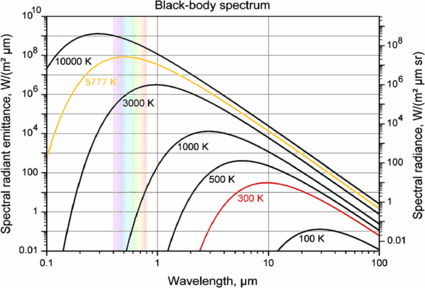

  

  Blackbody curves corresponding to different temperatures: the colder the temperature, the longer the wavelengths were the Planckians peak

In the first case, molecular signatures appear in absorption in front of the stellar background. On the contrary, in the thermal regime, the emitted flux refers to the temperature of the emitting layer, i.e. the atmospheric level where the optical depth is equal to 1. If the thermal profile decreases monotonically as the altitude increases (as in the case of Mars and Venus), molecular signatures appear in absorption. If a temperature inversion is present, i.e. if the exoplanet exhibits a stratosphere (as in the case of the Earth, giant planets and Titan), the molecular features may appear in emission or in absorption, depending on the atmospheric level where the lines are formed (see e.g. Encrenaz et al. 2004). Because we have no a priori information about the thermal profile of the exoplanet atmosphere, it is important to identify the wavelength range where each component (reflected or thermal) dominates.

5.1 Reflected/scattered stellar component and thermal emission

Figure 10a shows the two components (in the form of blackbody curves) for an exoplanet at various distances from a solar-type star, assuming an albedo of 0.3. If an albedo of 0.03 is chosen, the equilibrium temperatures are increased by about 10 % (see Table 1) and the curves of the thermal emission are slightly shifted toward shorter wavelengths. For a hot Jupiter located at 0.05 AU, the thermal emission dominates all wavelengths above 1.7 μm. At 1 AU, both components contribute equally around 5 μm. Note that in the case of the Earth, the actual temperature is 33 K warmer due to the greenhouse effect, and the crossover between the two components is shifted to 4 μm.

Fig. 10a

Reflected and thermal components in the case of a solar-type star

Figures 10b and 10c show the same plots for F-type and M-type stars, respectively. In the M star case, the reflected and thermal components are balanced at about 5 μm, 7 μm and 14 μm for distances of 0.05, 0.1 AU and 1 AU, respectively. Figures 11 and 12 show the same plots in a few specific cases: very hot objects (HAT-P-7b and CoRoT-1b), hot objects (HD209458b and HD189733b) and warm objects (GJ 436b and GJ 1214b). The crossover between the reflected and thermal components lies between 0.5 and 1 μm for very hot objects, between 1.0 and 1.5 μm for hot Jupiters and between 1.5 and 4 μm for warm objects.

Fig. 10b

Reflected and thermal components in the case of a F-type star

Fig. 10c

Reflected and thermal components in the case of a M-type star

Fig. 11

Reflected and thermal components for two sets of hot Jupiters: HAT-P-7b and CoRoT-1b (very hot objects, left) and HD209458b and HD189733b (most observed targets, right)

Fig. 12

Reflected and thermal components for two warm objects: GJ 436b and GJ 1214b. Calculations are made for two values of the albedo, a=0.3 and a=0.03

5.2 Which spectral range is best suited?

• Both the reflected and the thermal components show advantages and limitations. In the reflected component, the identification is easier (as all features appear in absorption) but no information can be extracted on the vertical distributions of species, or on temperature. In the thermal regime, one needs to retrieve simultaneously the thermal profile and the vertical profiles of the atmospheric species. Combining the analysis of both components, whenever feasible, will be of great help for characterising the atmosphere. This implies a spectral interval ranging from ∼0.4 μm (to include the maximum of the reflected flux of F-type stars) to 16 μm (to include the maximum emission of temperate objects around M-type stars). The planetary albedo and the surface properties can be measured only through the reflected component.

• Remote sensing of solar-system planetary atmospheres has demonstrated the importance of analysing, for a given species, multiple bands with different intensities. Redundancy may help resolving the ambiguities. Moreover, in the thermal regime, such bands probe different atmospheric levels, with the strongest ones being formed in the upper levels. Thanks to this information, the vertical structure of the atmosphere can be retrieved. This translates into the need of a wide spectral coverage for the thermal component.

• For temperate planets, the maximum of the emission peaks beyond 5 μm. It is therefore mandatory to extend the spectroscopic observations toward the mid-infrared to characterise these objects. The case of M stars is of special interest: these stars represent about 90 % of the total stellar population and given their smaller size compared to other main sequence stars, they are more favourable for transit observations.

5.3 Main molecular bands and constraints on the resolving power

5.3.1 The 2–18 μm range

We first consider wavelengths longer than 2 μm, which are best suited for several reasons: (1) spectral signatures are stronger because all molecules have their fundamental vibration–rotation bands in this range; (2) as mentioned above (Sect. 5.1), the planet to star flux ratio increases at longer wavelengths; (3) at wavelengths shorter than 2 μm, spectroscopic data for molecules—overtone and combination bands—are much less well known, especially at high temperature (see Sects. 5.3.2 and 5.3.5).

Table 5 shows a list of strong infrared bands in the 2–18 μm range for a series of possible candidate species. The first ones to be considered are H₂O, CH₄, NH₃, CO and CO₂. Figure 13 shows the strong effect of temperature on the shape of molecular bands (here H₂O and NH₃). For completion, we also consider C₂H₂ and C₂H₆, the two main products of methane photodissociation, observed in the solar-system giant planets, PH₃ (observed in Jupiter and Saturn), HCN (detected on Neptune) and O₃ (observed on Earth). Many weaker bands of all these species are also present, especially below 5 μm. Figure 14 shows a synthetic absorption spectrum of the five major species (H₂O, CH₄, NH₃, CO, CO₂) calculated under the same conditions (P=1 bar, column density=10 cm-amagat). For comparison, [H₂] = 30 km-amagat on Jupiter, [CH₄] = 50 m-amagat on Jupiter and [CO₂] = 100 m-amagat on Mars. Two temperatures are considered: T=300 K (temperate planets) and T=1200 K (hot planets). Figure 15 shows spectra of minor species, such as HCN, C₂H₂, C₂H₆, O₃, also at 300 K and 1200 K.

Fig. 13

Calculated line intensity for water vapour (top, Barber et al. 2006) and ammonia (bottom, Yurchenko et al. 2011) as a function of wavelengths and temperature. The figure shows how molecular opacities change in intensity and shape due to the temperature. This effect needs to be accounted for in spectral simulations

Fig. 14

Transmission of main candidate molecules (H₂O, CO₂, CO, CH₄, NH₃) between 2 and 18 μm. Calculations use a line-by-line model with, for each gas, a pressure of 1 atm and a column density of 10 cm-amagat. Top: T=300 K; bottom: T=1200 K. The spectral resolution is 10 cm⁻¹, which corresponds to a resolving power of 67 at 16 μm, 100 at 10 μm and 500 at 2 μm. The spectroscopic parameters are taken from the GEISA data base (Jacquinet-Husson et al. 2011)

Fig. 15

Transmission of minor species (HCN, C₂ H₂, C₂H₆, O₃) between 2 and 18 μm. The column density is 1 cm-amagat for each molecule. Top: T=300 K; bottom: T=1200 K. The pressure is 1 atm. The spectral resolution is 10 cm ⁻¹

Table 5 Main molecular signatures and constraints on the spectral resolving power. Δν is the spectral interval between two adjacent J-components of a band. S _max is the intensity of the strongest band available in the spectral interval. R is the spectral resolving power required to separate two adjacent J-components (Δν). Rotational constants, bands assignments and intensities are taken from Herzberg (1968), Townes and Schawlow (1975), Pugh and Rao (1976) and Rothman et al. (1983)

Most molecules exhibit two or more strong molecular bands in the 2–16 μm range, so both redundancy and the ability to retrieve a vertical structure are guaranteed. The second comment to be made is that spectral features are broadened at high temperature, due to the increasing contribution of high J-value components in each molecular band. On one hand they are detectable at lower spectral resolution, but if multiple molecular species overlap the identification becomes more difficult. For an unambiguous identification of a given molecule, the spectral resolving power should, ideally, be sufficient to separate two adjacent J-components of this molecule (Fig. 16). This interval is equal to 2B ₀, where B ₀ is the rotational constant of the molecule. Table 5 lists this interval Δν for the main bands of our list of candidate species, and the resolving power required to resolve this interval.

Fig. 16

Examples of synthetic spectra of H₂O, NH₃ and CH₄ in some of their fundamental bands, for two temperatures (300 K and 1200 K). The spectral resolution is 10 cm⁻¹, corresponding to a resolving power of 100 at 10 μm (NH₃ ν ₂ band), 150 at 6 μm (H₂O ν ₂ band) and 300 around 3 μm (H₂O ν ₁ and ν ₃ bands, CH₄ ν ₃ band). In all cases, the resolving power is sufficient to separate two adjacent J-components in each band

Two spectral domains are considered, the 2–5 μm and the 5–16 μm range. The molecular features, in fact, become stronger and less packed at wavelengths longer than 5 μm. The spectral separation of molecular bands above 5 μm is easier than at shorter wavelengths, because the overlap is less severe. We can see that for H₂O, CH₄ and their isotopes, as well as for NH₃ and PH₃, a resolving power of 300 (below 5 μm) and 150 (above 5 μm) is sufficient for identifying the bands unambiguously at any temperature.

Figure 17 shows the transmission of H₂O, CO₂, CH₄ and NH₃ between 5 and 18 μm, for a spectral resolution of 33 cm⁻¹, which corresponds to a resolving power of 20 at 16 μm, 30 at 10 μm and 60 at 5 μm. We appreciate that it is still possible to identify the main species through their general shapes, even at high temperature.

Fig. 17

Transmission of main candidate molecules (H₂O, CO₂, CO, CH₄, NH₃) between 5 and 18 μm, under the same conditions as in Figs. 7a, 7b. The spectral resolution is 33 cm⁻¹, which corresponds to a resolving power of 20 at 16 μm, 30 at 10 μm and 60 at 5 μm. Top: T=300 K; bottom: T=1200 K. It can be seen that the band shapes of all species remain separated even at high temperature (H₂O at 6.3 μm, CH₄ at 7.7 μm, NH₃ at 10.5 μm, CO₂ at 15.0 μm)

5.3.2 The 1–2 μm range

For temperate and warm objects, the 1–2 μm range is important to measure the reflected or scattered starlight of temperate objects. While many transit spectra of hot Jupiters have been observed in this spectral range using HST/NICMOS, HST/WFC3 and ground-based facilities, modelling exoplanetary spectra in this spectral range is complicated by the complexity of the molecular signatures. Many weak bands (typically overtone and combination bands) are present between 1 and 2 μm. Their spectroscopic identification is not complete, and the calculation of the opacities at high temperature is much more uncertain than at longer wavelengths.

Figure 18 shows a synthetic absorption spectrum of H₂O, CH₄, NH₃, CO₂, HCN and C₂H₂ calculated between 1 and 2 μm under the same conditions as in the 2–16 μm range (P=1 bar, column density = 10 cm-amagat; Fig. 14). The CO absorption (present in the (3-0) band at 1.57 μm is negligible at this scale. The spectral resolution (25 cm⁻¹) is adjusted to give a mean resolving power of 300, as in Fig. 13. Comparison of Figs. 14 and 18 illustrate that molecular absorptions are significantly weaker below 2 μm, and that detecting molecular species at longer wavelengths should be easier.

Fig. 18

Transmission of main candidate molecules (H₂O, CO₂, CH₄, NH₃, HCN, C₂H₂) between 1 and 2 μm. Conditions are the same as in Figs. 7a, 7b (P=1 bar, column density: 10 cm-atm). Top: T=300 K; bottom: T=1200 K. The spectral resolution is 25 cm⁻¹, which corresponds to a resolving power of 200 at 2 μm, 300 at 1.67 μm and 400 at 1 μm. The spectroscopic parameters are taken from the GEISA data base (Jacquinet-Husson et al. 2011). The data base is known to be incomplete, especially in the case of CH₄ (see text)

It should be emphasised that many molecular transitions are still missing in databases such as GEISA or HITRAN, especially in this wavelength interval. This issue is discussed in Sect. 5.3.5.

5.3.3 The visible range

For hot planets, opacities in the visible range are dominated by metallic resonance lines (Na at 0.59 μm, K at 0.77 μm, and weaker Cs transitions at 0.85 and 0.89 μm). Theoretical calculations of absorption profiles of Na and K perturbed by H₂ and He at high temperatures have been performed by Allard et al. (2003, 2012). Figure 19 shows a simulated visible spectrum of a gaseous, cloud-free exoplanet at spectral resolution R∼200. For cloud-free atmospheres, a resolving power of ∼100 is still sufficient for identifying the resonance lines of Na and K, but not to resolve the centre of the line.

Fig. 19

Synthetic transit spectra of a hot, gaseous exoplanet in the visible range, assuming a spectral resolution R∼200. The resonance lines are Na at 0.59 μm and K at 0.77 μm (calculated cross sections from Allard et al. 2003). Water vapour and methane spectral features are weaker here compared to the IR. We used calculated BT2 line list for water at high temperature (Barber et al. 2006) and methane absorption coefficients from Karkoschka and Tomasko (2010). The slope of the continuum is due to Rayleigh scattering by molecular hydrogen

In a cloud-free atmosphere, the continuum in the UV–VIS is given by Rayleigh scattering on the blue side, i.e. for wavelengths shorter than 1 micron (Rayleigh scattering varies as 1/λ ⁴). If there are clouds or hazes with small-size particles, those should be detectable in the visible. For small (particle diameter a≪λ), spherical particles the multiple scattering with the stellar photons can be simulated using Mie scattering approximation (e.g. Goody and Yung 1989). If the particles are larger (particle diameter a≥λ) or non-spherical, then the calculations are more complex (Liou 2002). Apart from the particle size and shape, the other important parameters are the particle distribution function and the pressure of the atmospheric layer where clouds/hazes form. From a radiative-transfer perspective, the composition is less important (De Kok and Stam 2012), and this explains why it is exceedingly difficult to retrieve clouds’ or hazes’ composition from remote sensing.

A key molecule absorbing in the visible range is molecular oxygen (Fig. 20, Pallé et al. 2009). A spectral resolving higher than 100 is needed to detect these features which are very narrow (see e.g. the A-band at 0.76 μm). In the Earth’s atmosphere the oxygen abundance is so high that even its dimer, O₄, and collisions between O₂ and N₂ are detectable in a disc-averaged spectrum (Tinetti et al. 2006a; Pallé et al. 2009). In the spectrum of the Earth shown in Fig. 20, ions are also present: Ca II H and K lines at 0.3934, 0.3968 μm, and the Ca II triplet at 0.8498, 0.8542 and 0.8662 μm.

Fig. 20

Earth’s transmission spectrum measured through lunar eclipse (Pallé et al. 2009). In the Earth’s atmosphere the oxygen’s abundance is so high that even its dimer, O₄, and collisions between O₂ and N₂ are detectable. Ions are also present: Ca II at 0.3934, 0.3968 μm, H and K lines at 0.8498, 0.8542 and 0.8662 μm

Atomic species such as He I (Moutou et al. 2001, 2003), Ca (Bundy and Marcy 2000; Narita et al. 2005; Shkolnik et al. 2005) and Fe (Bundy and Marcy 2000; Narita et al. 2005) have been sought in hot Jupiters atmospheres, but not yet detected in these planets.

5.3.4 A modelling of an exoplanet transit spectrum between 1 and 16 μm

As a summary of the above discussion, Figs. 21a and 21b show models of the expected contributions of a large number of molecules to the transit spectrum of a hot gaseous exoplanet between 1 and 16 μm (see equations in Sect. 2.1.1). The atmospheric temperature is assumed =800 K. Since we are interested in the relative molecular contributions here, the atmospheric absorption is normalised to 1; typically the fraction of stellar flux absorbed by the atmosphere of a hot, gaseous planet is 10⁻⁴–10⁻³. In addition to the main candidate absorbers (H₂O, CH₄, NH₃, CO, CO₂), calculations include contributions from HCN, O₃, H₂S, PH₃, SO₂, C₂H₂, C₂H₆ and $\mathrm{H}_{3}^{+}$. In Fig. 21a, two values (300 and 30) are used for the spectral resolving power. While R=30 is OK to detect most of the molecules at λ>5, especially at high temperatures, we would lose the possibility to resolve the CO₂, HCN and other hydrocarbons Q-branches. In Fig. 21b (R=300), it is worth noticing the possible signature of $\mathrm{H}_{3} ^{+}$ around 2 μm and 3–4 μm, easily detectable with a resolving power of ∼300. The $\mathrm{H}_{3} ^{+}$ ion, which plays a critical role in the cooling and stabilising of gaseous planets’ atmospheres (Maillard and Miller, 2012), has been detected in the ionospheres of Jupiter, Saturn and Uranus (Drossart et al. 1989; Geballe et al. 1993; Trafton et al. 1993), and its presence could be reasonably expected in the upper atmospheres of highly irradiated gaseous planets (Koskinen et al. 2007).

Fig. 21a

Absorptions contributions from different molecules in the transmission spectrum of a hot, gaseous exoplanet. Two values of the spectral resolving power are use: 300 (thin line) and 30 (thick line). The dashed vertical lines indicate the positions of maximum absorption for the different molecules. We used high temperature line lists BT2 (Barber et al. 2006) for water, BYTe (Yurchenko et al. 2011) for ammonia, Neale et al. (1996) coefficients for $\mathrm{H}_{3}^{+}$ and HITEMP (Rothman et al. 2010) for CO and CO₂. The other molecules were simulated using HITRAN 2008 (Rothman et al. 2013) line list

Fig. 21b

Enlargement of Fig. 13a in the 1–5 μm range, for a spectral resolving power of 300

5.3.5 Status of current databases for hot temperatures

The modelling of planetary and exoplanetary atmospheres requires extensive opacity databases. High-temperature spectroscopic data cannot be extrapolated from low temperature atmospheric database such as the most currently used HITRAN (Rothman et al. 2013) and GEISA (Jacquinet-Husson et al. 2011). Such extrapolations fail to reproduce high J rovibrational transitions and hot band transitions involving highly excited vibrational levels. The question of the opacity calculations at high temperature is discussed, in particular, by Sharp and Burrows (2007), Tinetti et al. (2012a) and Tennyson and Yurchenko (2012). Several databases already provide transitions line lists at high temperature (including positions and absorption cross sections) of a series of molecules of astrophysical and planetological relevance (BT2 for water (Barber et al. 2006; Fig. 13), CDSD-4000 for CO₂ (Tashkun and Perevalov 2011), as well as some hot spectra for NH₃ (Hargreaves et al. 2011; Yurchenko et al. 2011; Zobov et al. 2011; Fig. 13), HCN (Harris et al. 2008; Mellau 2011) and CH₄ (Nassar and Bernath 2003; Thiévin et al. 2008; Hargreaves et al. 2012; Yurchenko et al., in prep.)). Several of these line lists are assembled in the databases EXOMOL (Tennyson and Yurchenko 2012) and HITEMP (Rothman et al. 2010). Most of these databases will be soon available through the common portal built within the Framework of the VAMDC (Virtual Atomic and Molecular Data Centre) European Network (Dubernet et al. 2010).

At present, accurate molecular models are still missing to generate complete high temperature line lists for polyatomic absorbers, such as small hydrocarbons as CH₄, C₂H₂, C₂H₄ or C₂H₆ and the C-containing transient species (C₂H, CH₂, C₃, C₄) which dominate the opacity of Brown Dwarfs, exoplanets and AGBs and play a primary role in the physical-chemistry of their outer atmospheres. We list them here:

CH₄—After water, methane is one of the most important opacity sources in the layers of exoplanets (Sudarsky et al. 2000; Swain et al. 2008, 2009a, 2009b; Tinetti et al. 2010) as well as in those of Brown Dwarfs (e.g. Allard et al. 1997; Burgasser et al. 2006; Nakajima et al. 2004). Methane fluorescence has also been observed in the emission spectrum of an exoplanet (Swain et al. 2010; Waldmann et al. 2012). The strong transition of methane at 3 μm completely dominates the spectrum of BDs at 1600 K and is still identifiable at 1800 K (Borysow et al. 2002). Statistical narrow-band models (Perrin et al. 2007), ab initio models (Warmbier et al. 2009; Yurchenko et al., in preparation) or extrapolations from global effective models (Wenger et al. 2008) have been proposed to reproduce the low resolution spectrum of CH₄ up or above 2000 K. From an experimental point of view, Nassar and Bernath (2003) measured line absorption cross sections up to 1273 K. Measurements of line absorption cross sections up to 1850 K in the 3 μm region were published by Thiévin et al. (2008). Karkoschka and Tomasko (2010) have collected low temperature laboratory and planetary measurements to estimate methane transmission in the 0.4–5.5 μm wavelength interval. Most recently Hargreaves et al. (2012) have published experimental line lists of methane at high temperatures (300–1400 ^∘C) spanning the 2–10.4 μm region.

C₂H₆—Ethane is the second most abundant hydrocarbon in giant planet atmospheres and in low-mass BDs, so-called T-dwarfs. Thermochemical equilibrium computations indicate that several compounds may be useful to establish temperature or pressure scales for giant planets, Brown Dwarfs or dwarf star atmospheres (Lodders and Fegley 2002). For giant planets and warm methane dwarfs, such as Gl 229B, the deep atmospheric abundance of ethane is a diagnostic temperature probe. This species could be very useful as temperature probe but high temperature data are missing. The available absorption cross sections of ethane in the IR were recorded at low and room temperatures only (Harrison et al. 2010).

C₂H₂—The strong contribution of the 3 μm and 13.7 μm acetylene bands is predicted by opacity models of AGB stars to prevail up to 2000 K. Moreover, recent photochemical models (Zahnle et al. 2010) suggest that large amounts of carbon molecules in the form of polycyclic aromatic hydrocarbons (PAHs) and soot are present in the upper layers of the envelope of hot Jupiters, such as in HD189733b. PAHs have strong spectral signatures at 3.3 μm and at 6–7 μm which could be searched for. In addition, a diagnostic test that would confirm the presence of these compounds in their envelope is the detection of acetylene (Mousis et al. 2011). A new experimental approach based on the use of a novel high enthalpy source (Thiévin et al. 2008) allowed to measure high temperature emission spectra of acetylene in the 3 μm range, up to 1455 K, under Doppler limited resolution. These data, including the complete sequence of hot bands accessing vibrational states up to 8900 cm⁻¹, were incorporated in an effective global rovibrational Hamiltonian which is now able to simulate precise synthetic spectra up to 2000 K (Amyay et al. 2011).

C₂H₄—The emission of AGBs is partly affected by ethylene (C₂H₄) which has been detected in the outer shell of IRC+1021641 and IRL61842. Zahnle et al. (2010) and Stevenson et al. (2010) propose that methane combustion may generate C₂H₄ and HCN. Spectroscopic data are not yet reported at T higher than room temperature.

Transient species—A large number of unstable, unsaturated carbon chain radicals and/or ions have been identified in astrophysical objects including the molecular families HC _x and H₂C _x (Cernicharo et al. 2001), C _x (Bernath et al. 1989; Giesen et al. 2001). However, the spectroscopy of most of these species remains very incomplete. Several IR bands have yet to be measured in the laboratory; in particular the low frequency bending modes have never been obtained experimentally except for a few samples. It would be useful to have direct measurements of rotationally resolved low frequency vibrations and pure rotation transitions of C₃, C₄, C₂H and CH₂ in order to support the observations of Herschel and ALMA facilities and to model the high temperature IR spectra of these species. For $\mathrm{H}_{3}^{+}$ in particular, there is a good line list from Neale et al. (1996).

6 Searching for habitability using transit spectroscopy

6.1 Where to look for habitable exoplanets?

An ultimate objective for exoplanets’ exploration is the search for habitable worlds. In analogy with the conditions of life appearance on Earth, biologists have selected a few criteria to be fulfilled to have life on extraterrestrial worlds: these criteria are the simultaneous presence of carbon, liquid water and a source of energy. Astronomers have defined the concept of habitable zone (HZ) to determine the region where water can be liquid at the surface of an exoplanet: it corresponds to temperatures ranging typically between 250 and 380 K. In the case of solar-type stars, the lower boundary of the HZ is defined by water loss and the presence of a runaway greenhouse effect, while its outer boundary is defined by CO₂ condensation. The resulting boundaries are then 0.75–0.95 AU for the inner side and 1.37–1.77 AU for the outer side (Kasting et al. 1993).

As mentioned in previous sections, we have already a handful of terrestrial exoplanets in the temperate regime, i.e. potentially inside the habitable zone of its star, but none transiting yet, unless Kepler-22b is confirmed being a super-Earth.

6.2 Spectroscopic biosignatures

The acquisition of spectroscopic data of the Earth’s atmosphere from artificial satellites has changed our perception of terrestrial life and has provided a rigorous scientific framework to search for life elsewhere in our Galaxy. Seen from the outside, our planet appears to be similar, for some aspects, to other planets, yet it shows distinctive signatures of a life-hosting planet, which cannot be found elsewhere in the Solar System (Hanel et al. 2003).

Lovelock (1965) and Hitchcock and Lovelock (1967) suggest to search for the presence of compounds in the planet’s atmosphere which are incompatible on a long-term basis, i.e. in chemical disequilibrium. For example, oxygen and hydrocarbons co-exist in the Earth’s atmosphere.

Molecular oxygen was proposed as a biomarker by Owen (1980) and O₂ can be identified through its 760 nm band. This spectral signature is rather weak, though, and ozone, a photodissociation product of oxygen, appears to be a better tracer, thanks to its strong spectral signature at 9.6 μm (Angel et al. 1986; see Sect. 5.3.1).

However, oxygen in large quantities is more a tracer of “complex life”: in the case of the Earth, life appeared in the oceans about 1.5 Gy before the apparition of atmospheric oxygen (Rye and Holland 1998). Before the apparition of oxygen, anaerobes explored various types of metabolisms (methanogens, acetogens, sulphate/sulphur/iron/manganese reducers etc.), generating different products in the process (Nealson and Stahl 1997). In principle, all these products (e.g. CH₄, CH₃COOH, H₂S, Fe²⁺, MN²⁺, etc.) could be considered as biomarkers, but to be detected from space, they need to be very abundant and not explainable by other abiotic processes, which is often difficult to discern. For instance, on Earth, most of the methane comes from the decomposition of living organisms, on the other hand, on Titan the high abundance of methane is certainly not of biogenic source. N₂O is generated by biomass burning; however its spectral signatures are very weak compared with the above-mentioned molecules: in the infrared, the spectrum of the Earth is entirely dominated by water vapour signatures (Fig. 22).

Fig. 22

The spectrum of the Earth between 1 and 5 μm, recorder by the Near-infrared Mapping Spectrometer of the Galileo spacecraft during its flyby of the Earth in December 1990. The reflected solar component dominates at short wavelengths, and thermal emission prevails in the infrared range beyond 3 μm. In spite of the very low mixing ratio of water in the terrestrial atmosphere (less than 0.1 %), the spectrum is entirely dominated by H₂O, with minor contributions from CO₂ and marginal signatures from O₃, N₂O and CH₄. The figure is taken from Drossart et al. (1993)

The simultaneous detection of CH₄ and O₃ could provide a more convincing indication of life on an exoplanet (Selsis et al. 2008). The MIR wavelength range appears to be essential for this research. Indeed, all key molecules have very strong signatures in this range: O₃ at 9.6 μm, CH₄ at 7.7 μm, CO₂ at 15.0 μm and H₂O at 6.2 μm (see Sect. 5.3.1). Figure 23 shows that O₃ is detectable only on Earth, while CO₂ is present in the atmospheres of Venus, Earth and Mars.

Fig. 23

Thermal spectra of Venus (top), the Earth (middle) and Mars (bottom). The Venus data are from Venera 15 Fourier Transform Interferometer (Moroz et al. 1986). The Earth and Mars spectra are from NIMBUS 4 and Mariner 6, respectively (Hanel et al. 1992). The strong CO₂ band at 15 μm (667 cm⁻¹) is present on all planets. Ozone clearly appears at 9.7 μm (1040 cm⁻¹) in the Earth spectrum; H₂O and CH₄ are also visible around 20 μm (500 cm⁻¹) and 7.7 μm (1400 cm⁻¹), respectively. In the case of the Earth, an emission core appears at the centre of the absorption features, due to the temperature inversion in the Earth atmosphere. The figure is taken from Hanel et al. (1992)

On Earth, a sharp increase in the reflectivity at wavelengths above 0.7 μm is a distinctive signature of the vegetation, called the Red Vegetation Edge (RVE). That was observed in the near-infrared spectrum recorded by the Galileo spacecraft during its Earth flyby (Sagan et al. 1993). While this signature has been proposed as a possible biomarker on exoplanets (Woolf et al. 2002; Arnold et al. 2002; Seager et al. 2005; Montañés Rodríguez et al. 2006; Sterzik et al. 2012), caution is needed to avoid false positives: clouds or surface properties may mimic the spectral shape of the RVE.

6.3 Habitable exoplanets around M-type stars

Among the super-Earths discovered, we have already potential candidates for habitability, e.g. GJ 581d (Mayor et al. 2009) and GJ 667Cc (Anglada-Escudé et al. 2012). Interestingly, these planets do not orbit a canonical G-star, but rather a much dimmer and colder M-dwarf, clearly challenging any geocentric concept of habitability. We should expect many more planets like GJ 581d and GJ 667Cc in the future, given that 90 % of the stars in the solar neighbourhood are M-dwarfs and, from preliminary analysis of Kepler, small planets are seven times more abundant around cool stars (Howard et al. 2013). This represents a paradigm shift in the search for habitable worlds outside our Solar System, a search that started with the “Earth-twin” obsession.

As M-type stars have an intrinsically low luminosity, their habitable zone is located at close distances, typically at 0.1–0.3 AU (Segura et al. 2005). These objects are thus ideally suited for transit observations. In addition, the planet/star flux contrast is higher (see Sect. 2.2). Tidal locking is expected to induce superrotation, possibly observable from phase-curve observations. As the stellar spectrum of the M-star is redshifted compared with the solar one, Rayleigh scattering (proportional to λ ⁻⁴) is decreased, as well as the albedo of the planet. The increased magnetic activity of M-stars may lead to a stronger stellar wind, more stellar flares and possibly more atmospheric erosion (Lammer et al. 2007; Penz et al. 2008).

Joshi et al. (1997) and Wordsworth et al. (2011) have used three-dimensional simulations to estimate the climate and habitability of terrestrial planets in orbit around M stars. They conclude that not only M-dwarf planets can support an atmosphere over a range of conditions, but even habitability in some cases.

Based on knowledge of photosynthesis on Earth and of stellar evolution, Wolstencroft and Raven (2002) conclude that it is likely that photosynthesis would have evolved on Earth-like planets in response to the same evolutionary factors as have been involved on Earth. Their model of photosynthesis on Earth-like planets orbiting stars of different spectral types shows that cooler stars, with maximum radiation output at longer wavelengths, may require more than the 2 photons per electron that are transferred and that are used in oxygen-evolving photosynthesis on Earth. Detection of photosynthesis will be based on spectroscopy using most probably photosynthetic pigments that could have very different absorption properties from those on Earth. On a more speculative note, for M-dwarf planets one would expect that the “exovegetation” is responsible for producing a red-edge–like signature that is redshifted with respect to that of Earth’s vegetation (Tinetti et al. 2006b; Kiang et al. 2007).

7 The future: prospects from the ground and space

Spectroscopic characterisation of exoplanetary atmospheres is today restricted to bright targets, i.e. potentially to ∼150 targets. Ground-based telescopes have been used to cover the VIS/near-infrared spectral range, the Hubble Space Telescope from the UV to the near-IR and the Spitzer Space Telescope the mid-infrared.

Future prospects include new ground-based facilities and space projects (Fig. 24) described hereafter. Ideally these projects should include both general purpose facilities with large collective areas (JWST, SPICA, E-ELT, TMT etc.) and small/medium class dedicated space missions conceived to optimise the wavelength covera ge and observational strategy (EChO). Both these approaches have advantages and weaknesses: being able to use them in synergy would be an asset for this field.

Fig. 24

In the next decade important new facilities are foreseen with relevance to exoplanetary science

The 40-m E-ELT is under development at ESO (Kissler-Patig and Luybenova 2011; Liske et al. 2011), with an expected first light in 2022. Two instruments have been selected and are presently under study: ELT-CAM (MICADO), an infrared camera design to exploit the diffraction limit of the telescope (5 milliarcsec at 1 μm), and ELT-IFU, an integral field spectrometer working in the 0.47–2.46 μm range with resolving powers ranging from 4000 to 20000, based on the heritage of the SINFONI instrument at the VLT; ELT-IFU should be well suited for measuring spectra of transiting exoplanets now detected with 10-m telescopes. The third planned instrument is ELT-MIR (METIS), an infrared instrument (2.9–14 μm) designed for the spectroscopy of transiting exoplanets in the L, M and N bands (Brandl et al. 2008). The following planned instrument will be either a multi-object spectrograph (ELT-MOS) or a visible/near IR high-resolution spectrometer (ELT-HIRES); the latter would be primary designed for the search for exoplanets by radial velocity.

The James Webb Space Telescope, developed by NASA with ESA participation, is expected to be in operation beyond 2018. Two infrared imaging spectrometers of special interest for transit spectroscopy of exoplanets will be mounted on its 6.5 m telescope. The Near Infrared Spectrometer NIRSpec (Gardner et al. 2006) will cover the 0.6–5 μm range with a spectral resolving power of a few thousands. The MIRI infrared camera (Wright et al. 2003) will cover the 5–28 μm range using different modes with high and low spectral resolutions. Sensitivity calculations for exoplanet characterisation have been performed e.g. by Seager et al. (2009), Kaltenegger and Traub (2009), Clampin (2010), Deming et al. (2010), Belu et al. (2011) and Rauer et al. (2012).

Having a large collective area, i.e. more photons, is certainly very positive, but the lesson learnt from Spitzer and Hubble is that other aspects may be as critical, e.g. the instrument’s stability and the knowledge of the instrument systematics. Kepler has been an incontestable success because it was built from start to achieve the 10⁻⁴ to 10⁻⁵ photometric precision needed to discover Earth-size planets. Another critical point is the stellar activity, which often forbids the possibility of combining measurements at different wavelengths, if recorded at different times. Moreover, instruments are most of the time not calibrated at the level needed to combine multiple observations. The ability to observe simultaneously a broad wavelength range, permits to solve these issues.

The EChO mission (Exoplanet Characterisation Observatory) is being assessed by ESA as one of the five ESA-M3 mission candidates, competing for a launch in 2022. EChO is a 1.2 m telescope to be placed in L2, designed to observe repeatedly a rich sample of exoplanets over a very extended wavelength range (0.5–16 μm) in a single run (Tinetti et al. 2012a, 2012b). The objective of EChO is to explore spectroscopically a large variety of objects, from hot to temperate, including Jupiters, Neptunes and super-Earths. The duration of the mission will be at least 4 years. Sensitivity studies were performed by Tessenyi et al. (2012, 2013), and Barstow et al. (2013). They show that optimal spectroscopic observations require F, G and K stellar targets brighter than V=12 and M stars brighter than K=9. There are presently over 150 existing sources which fulfil these conditions, and more favourable targets are expected to be discovered in the coming years before the launch of the mission.

8 Conclusions

Little more than ten years ago, the detection of a signal from an exoplanet atmosphere was still in the realm of science fiction. Pioneering results were then obtained through primary transits in the UV and visible range, using the Hubble Space Telescope/STIS instrument. These were later extended towards the infrared, making possible the detection of molecular species and of the planet’s thermal emission. Key instruments have been the IRAC camera and the IRS spectrometer on board the Spitzer satellite and the Hubble NICMOS spectrograph and WFC3 camera. Important contributions have also come from ground-based instruments, in particular CRIRES on the VLT, the infrared spectrometer NIRSPEC on the Keck, and the imaging spectrometer SpeX at IRTF. Ground-based facilities offer specific niches for focussed observations, often unfeasible from space.

The exploration of transiting exoplanets has revealed an incredible variety of objects, exceeding by far what we could expect based on our own solar system. Such a variety begs to observe their atmospheric chemical composition. Results obtained over the past ten years on a few hot Jupiters already illustrate that these objects are much more complex than expected: their atmospheric composition, in fact, cannot be explained by simple thermochemical equilibrium calculations. The simultaneous presence of CO₂ and CH₄, for instance, indicates that other physical processes, most likely transport-induced quenching and photochemistry, are at work.

The difficulty in retrieving simultaneously the thermal profile and the chemical abundances can be addressed by using both primary transits and secondary eclipses, and by extending the spectral range as much as possible, to benefit from the simultaneous observation of multiple bands for a given species. Infrared spectroscopic data—measured of calculated—of methane, ethylene and ethane between 500 and 3000 K, will be critical to improve the interpretation of the observed spectra.

The few available transit spectra of hot Jupiters are comparable in quality with the Solar System planetary spectra known in the 1970s, before the Voyager era. With the arrival of larger telescopes or dedicated instruments in the coming decade, planetary science will expand beyond the narrow boundaries of our Solar System to encompass our whole Galaxy.

References

Ackerman AS, Marley MS (2001) Precipitating condensation clouds in substellar atmospheres. Astrophys J 556:872–884
Adams FC (2011) Magnetically controlled outflows from hot Jupiters. Astrophys J 730(1):27. 17 pp.
Adams ER et al. (2008) Ocean planet or thick atmosphere: on the mass-radius relationship for solid exoplanets with massive atmospheres. Astrophys J 673:1160
Agol E, Cowan NB, Knutson HA et al. (2010) The climate of HD189733 b from fourteen transits and eclipses measured by Spitzer. Astrophys J 721:1861–1877
Alibert Y, Mordasini C, Benz W et al. (2005) Models of giant planet formation with migration and disk evolution. Astron Astrophys 434:343–353
Allard F, Hauschildt PH, Alexander DR et al. (1997) Model atmospheres of very low mass stars and brown dwarfs. Annu Rev Astron Astrophys 75:137–177
Allard NF, Allard F, Hauschildt PH, Kielkopf JF, Machin L (2003) A new model for brown dwarf spectra including accurate unified line shape theory for the Na I and K I resonance line profiles. Astron Astrophys 411:L473–L476
Allard NF et al. (2012) Theoretical and laboratory spectra of sodium perturbed by molecular hydrogen. Astron Astrophys 543:A159
Amyay B, Fayt A, Herman M (2011) Accurate partition function for acetylene, 12C2H2 and related thermodynamical quantities. J Chem Phys 135:234305
Angel JRP, Cheng AYS, Woolf NJ (1986) A space telescope for infrared spectroscopy of Earth-like planets. Nature 322:341–343
Anglada-Escudé G, Arriagada P, Vogt SS et al. (2012) A planetary system around the nearby M dwarf GJ667 c with at least one super-Earth in its habitable zone. Astrophys J 751:L16
Arnold L, Gillet S, Lardière O et al. (2002) A test for the search for life on extrasolar planets. Looking for the terrestrial vegetation signature in the Earthshine spectrum. Astron Astrophys 392:231–237
Atreya SK, Mahaffy PR, Niemann HB, Wong MH, Owen TC (2003) Composition and origin of the atmosphere of Jupiter—an update, and implications for the extrasolar giant planets. Planet Space Sci 51:105-112
Atreya SK, Lorentz RD, Waite JH (2010) Volatile origins and cycles. In: Brown RH, Lebreton J-P, Waite JH (eds) Titan from Cassini–Huygens. Springer, Berlin, p 177. ISBN 978-1-4020-9214-5.
Barber RJ, Miller S, Tennyson J, Harris GJ, Tolchenov RN (2006) A high accuracy computed water line list. Mon Not R Astron Soc 368:1087–1094
Barman TS (2007) Identification of absorption features in an extrasolar planetary atmosphere. Astrophys J 661:L191, L194
Barman TS (2008) On the presence of water and global circulation in the transiting planet HD189733 b. Astrophysics 676:L61–L64
Barman TS et al. (2011) Clouds and chemistry in the atmosphere of extrasolar planet HR8799b. Astrophys J 733(1):65. 18 pp.
Barstow JK et al. (2013) On the potential of the EChO mission to characterise gas giant atmospheres. Mon Not R Astron Soc 430(2):1188–1207
Batalha NM et al. (2011) Kepler’s first rocky planet: Kepler-10b. Astrophys J 729(1):27. 21 pp.
Batalha N et al. (2013) Planetary candidates observed by Kepler, III: Analysis of the first 16 months of data. Astrophys J Suppl Ser 204:24
Bean JL, Miller-Ricci E, Homeier D (2010) A ground-based transmission spectrum of the super-Earth exoplanet GJ 1214 b. Nature 468:669–672
Bean JL, Desert J-M, Kabath P et al. (2011) The optical and near-infrared transmission spectrum of the Super-Earth GJ 1214b: further evidence for a metal-rich atmosphere. Astrophys J 743:92
Beaulieu JP et al. (2006) Discovery of a cool planet of 5.5 Earth masses through gravitational microlensing. Nature 439(7075):437–440
Beaulieu JP, Carey S, Ribas I et al. (2008) Primary transit of the planet HD189733 b at 3.6 and 5.8 micron. Astrophys J 677:1343–1347
Beaulieu J-P, Kipping DM, Batista V et al. (2010) Water in the atmosphere of HD209458b from 3.6–8 μm IRAC photometry observations in primary transits. Mon Not R Astron Soc 409:963–974
Beaulieu J-P, Tinetti G, Kipping DM et al. (2011) Methane in the atmosphere of the transiting hot Neptune GJ436 b? Astrophys J 731:16
Belu AR, Selsis F, Morales J-C, Ribas I, Cossou C, Rauer H (2011) Primary and secondary eclipse spectroscopy with JWST: exploring the exoplanet parameter space. Astron Astrophys 525:A83
Ben-Jaffel L (2007) Exoplanet HD209458 b: hydrogen inflated atmosphere but no sign of evaporation. Astrophys J 671:L61–L64
Ben-Jaffel L (2008) Spectral, spatial, and time properties of the hydrogen nebula around exoplanet HD209458b. Astrophys J 688:1352–1360
Ben-Jaffel L, Hosseini SS (2010) On the existence of energetic atoms in the upper atmosphere of exoplanet HD209458b. Astrophys J 709:1284–1296
Bernath PF, Hinkle KH, Keady JJ (1989) Detection of C5 in the circumstellar shell of IRC10216. Science 144:562–564
Berta ZK, Charbonneau D, Désert J-M et al. (2012) The flat transmission spectrum of the super Earth GJ 1214 b from Wide Field Camera 3 on the Hubble Space Telescope. Astrophys J 747:35
Bethe HA (1939) Energy production in stars. Phys Rev 55(5):434–456
Borucki WJ, Koch D, Jenkin J et al. (2009) Kepler’s optical phase curve of the exoplanet HAT-P-7 b. Science 325:709
Borucki WJ et al. (2011) Characteristics of planetary candidates observed by Kepler. II. Analysis of the first four months of data. Astrophys J 736:19
Borucki WJ, Koch DG, Batalha N et al. (2012) Kepler-22 b: a 2.4 Earth-radius planet in the habitable zone of a sun-like star. Astrophysics 745:120
Borysow A, Jorgensen UG, Fu Y (2001) High-temperature (1000–7000 K) collision-induced absorption of H2 pairs computed from the first principles, with application to cool and dense stellar atmospheres. J Quant Spectrosc Radiat Transf 68:235
Borysow A, Champion JP, Joergensen UG, Wenger C (2002) Toward simulation of high temperature methane spectra. Mol Phys 22:3585–3594
Boss A (1997) Giant planet formation by gravitational instability. Science 276:1836–1839
Boss A (2005) Evolution of the solar nebula. VII. Formation and survival of protoplanets formed by disk instability. Astrophys J 629:535–548
Brandl B, Lenzen R, Pantin E et al. (2008) METIS: the mid-infrared E-ELT imager and spectrograph. In: McLean IS, Casali M (eds) Ground-based and airborne instrumentation for astronomy II. Proceedings of the SPIE, vol 7014, pp 70140–70141
Bracewell AN (1978) Detecting nonsolar planets by spinning infrared interferometer. Nature 274:780–781
Brogi M, Snellen IAG, de Kok RJ et al. (2012) The signature of orbital motion from the dayside of the planet τ bootis b. Nature 486:502–504
Brown TM (2001) Transmission spectra as diagnostics of extrasolar giant planet atmospheres. Astrophys J 553:1006
Bundy KA, Marcy GW (2000) A search for transit effects in spectra of 51 Pegasi and HD 209458. Publ Astron Soc Pac 112(777):1421–1425
Burgasser AJ, Geballe TR, Leggett SK, Kirkpatrick JD, Golimowski DA (2006) A unified near-infrared spectral classification scheme for T dwarfs. Astrophys J 637(2):1067–1093
Burke CJ, McCullough PR, Bergeron LE et al. (2010) NICMOS observations of the transiting hot Jupiter XO-1b. Astrophys J 719:1796–1806
Burrows A, Sharp CM (1999) Chemical equilibrium abundances in brown dwarf and extrasolar giant planets atmospheres. Astrophys J 512:843–863
Burrows A, Hubeny I, Budaj J et al. (2007) Theoretical spectral models of the planet HD209458b with a thermal inversion and water emission bands. Astrophys J 668:L171–L174
Burrows A, Budaj J, Hubeny I (2008) Theoretical spectra and light curves of close-in extrasolar giant planets and comparison with data. Astrophys J 678(2):1436–1457
Burrows A, Rauscher E, Spiegel DS, Menou K (2010) Photometric and spectral signatures of three-dimensional models of transiting giant exoplanets. Astrophys J 719:341–350
Cameron AGW (1978) Physics of the primitive solar accretion disk. Moon Planets 18:5–40
Carter JA, Winn JN (2009) Parameter estimation for time-series data with correlated errors: a wavelet-based method and its application to transit lightcurve. Astrophys J 704:51–57
Casertano S, Lattanzi MG, Sozzetti A et al. (2008) Double-blind test program for astrometric planet detection with Gaia. Astron Astrophys 482:699
Cassan A et al. (2012) One or more bound planet per Milky Way star from microlensing observations. Nature 481:167–169
Cernicharo J, Heras A, Tielens AGGM et al. (2001) Infrared Space Observatory’s discovery of C4H2, C6H2 and benzene in CRL 618. Astrophys J 546:L123–L126
Chandrasekhar S (1960) Radiative transfer. Dover, New York
Charbonneau D, Brown TM, Lantham DW et al. (2000) Detection of planetary transits across a Sun-like star. Astrophys J 529:L45–L48
Charbonneau D, Brown TM, Noyes RW, Gilliland RL (2002) Detection of an extrasolar planet atmosphere. Astrophys J 568:377–384
Charbonneau D, Allen LE, Megeath ST et al. (2005) Detection of thermal emission from an extrasolar planet. Astrophys J 626:523–529
Charbonneau D, Knutson HA, Barman T et al. (2008) The broad-band infrared emission spectrum of the exoplanet HD189733 b. Astrophys J 686:1341–1348
Charbonneau D, Berta ZK, Irwin J et al. (2009) A super-Earth transiting a nearby low-mass star. Nature 462:891–894
Cho JYK, Menou K, Hansen BMS et al. (2003) The changing face of extrasolar planet HD209458 b. Astrophys J 587:L117–L120
Cho JY-K, Menou K, Hansen BMS, Seager S (2008) Atmospheric circulation of close-in extrasolar giant planets. I. Global, barotropic, adiabatic simulations. Astrophys J 675:817
Clampin M (2010) Pathways toward habitable planets: JWST’s capabilities for exoplanet science. In: Coudé du Foresto V, Gelino DM, Ribas I (eds) Pathways toward habitable planets. Astron soc of the pacific conference series, vol 430, pp 167–174
Cohen O, Glocer A (2012) Ambipolar electric field, photoelectrons, and their role in atmospheric escape from hot Jupiters. Astrophys J 743:L4.
Colon KD, Ford EB, Lee B et al. (2010) Characterizing transit extrasolar planets with narrow-band photometry and GTC/OSIRIS. Mon Not R Astron Soc 408:1494–1501
Cooper CS, Showman AP (2005) Dynamic meteorology at the photosphere of HD 209458B. Astrophys J 629:L45
Cooper CS, Showman AP (2006) Dynamics and disequilibrium carbon chemistry in hd 209458b’s atmosphere. Astrophys J 649:1048
Coustenis A, Taylor FW (1999) Titan, the Earth-like moon. World Scientific, Singapore
Coustenis A, Scheider J, Bockelée-Morvan D et al. (1997) Spectroscopy of 51 Peg b: search for atmospheric signatures. In: Planets beyond the solar system and the new generation of space mission. ASP, vol 119, p 101
Cowan NB, Agol E, Charbonneau D (2007) Hot nights on extrasolar planets: mid-infrared variations of hot Jupiters. Mon Not R Astron Soc 379:641–646
Croll B, Albert L, Jayawardhana R et al. (2011) Broadband transmission spectroscopy of the super-Earth GJ 1214b suggests a low mean molecular weight atmosphere. Astrophys J 736:78
Crossfield IJM, Hansen BMS, Harrington J et al. (2010) A new 24 micron phase curve for Upsilon Andromedae b. Astrophys J 723:1436–1446
Crossfield IJM, Barman T, Hansen BMS (2011) High resolution, differential, near-infrared transmission spectroscopy of GJ 1214b. Astrophys J 736:132
Crouzet N, McCullough PR, Burke C, Long D (2012) Transmission spectroscopy of exoplanet XO-2b observed with HST NICMOS. Astrophys J 761:7
Currie T et al. (2011) A combined Subaru/VLT/MMT 1–5 μm study of planets orbiting HR 8799: implications for atmospheric properties, masses, and formation. Astrophys J 729(2):128
Danielski C et al. (2012) 0.94–2.42 micron ground-based transmission spectra of the hot-Jupiter HD-189733b. Astrophys J (submitted). arXiv:1212.1206
De Kok RJ, Stam DM (2012) The influence of forward-scattered light in transmission measurements of (exo)planetary atmospheres. Icarus 221(2):517–524
De Kok RJ et al. (2013) Detection of carbon monoxide in the high-resolution day-side spectrum of the exoplanet HD 189733b. Astron Astrophys 554:A82. 9 pp.
De Wit J, Gillion M, Demory BO, Seager S (2012) Secondary eclipse scanning of HD189733 b: the perspectives of mapping distant worlds. Astron Astrophys 548:128
Deeg HJ, Moutou C, Erikson A et al. (2010) A transiting giant planet with a temperature between 250 and 430 K. Nature 464:384–387
Deming D, Seager D, Richardson LJ et al. (2005) Infrared radiation from an extrasolar planet. Nature 434:740–743
Deming D, Harrington J, Seager S et al. (2006) Strong infrared emission from the extrasolar planet HD189733 b. Astrophys J 644:560–564
Deming D et al. (2010) Discovery and characterization of transiting super earths using an all-sky transit survey and follow-up by the James Webb Space Telescope. Publ Astron Soc Pac 121(883):952–967
Deming D et al. (2013) Infrared transmission spectroscopy of the exoplanets HD209458B and XO-1B using the Wide Field Camera-3 on the Hubble Space Telescope. Astrophys J 774(2):95, 17 pp.
Désert J-M, Bean J, Miller-Ricci E et al. (2011) Observational evidence for a metal-rich atmosphere on the super-Earth GJ1214 b. Astrophys J 731:L40
Dobrovolskis AR (2013) Insolation on exoplanets with eccentricity and obliquity. Icarus 226(1):760–776
Dougherty MK et al. (2012) Jupiter ICy moons Explorer (JUICE): an ESA L-class mission candidate to the Jupiter system. In: 43rd Lunar and Planetary Science Conference. LPI Contribution No. 1659, id. 1806
Drossart, P. et al. (1989) Detection of H3(+) on Jupiter. Nature 340:539–541. Aug. 17
Dubernet ML et al. (2010) Virtual atomic and molecular data centre. J Quant Spectrosc Radiat Transf 111(15):2151–2159
Dyson F (1979) Time without end: physics and biology in an open universe. Rev Mod Phys 51
Eddington AS (1924) On the relation between the masses and luminosities of the stars. Mon Not R Astron Soc 84:308–332
Ehrenreich D, Tinetti G, Lecavelier des Etangs A, Vidal-Madjar A, Selsis F (2006) The transmission spectrum of Earth-size transiting planets. Astron Astrophys 448:379–393
Encrenaz T (2009) Water in the solar system. Annu Rev Astron Astrophys 46:57–87
Encrenaz T (2010) Characterizing exoplanet atmospheres and surfaces. In: Coudé du Foresto V, Gelino DM, Ribas I (eds) Pathways toward habitable planets. Astron soc of the pacific conference series, vol 430, pp 65–75
Encrenaz T, Bibring JP, Blanc M et al. (2004) The solar system, 3rd edn. Springer, Berlin
Feroz F, Balan ST, Hobson MP (2011) Bayesian evidence for two companions orbiting HIP 5158. Mon Not R Astron Soc 416:L104–L108
Forget F, Wordsworth RD (2010) Habitability of planets. In: Coudé du Foresto V, Gelino DM, Ribas I (eds) Pathways toward habitable planets. Astron soc of the pacific conference series, vol 430, pp 55–64
Fortney JJ, Marley MS, Barnes JW (2007) Planetary radii across five orders of magnitude in mass and stellar insolation: application to transits. Astrophys J 659(2):1661–1672
Fortney JJ, Lodders K, Marley MS et al. (2008) A unified theory for the atmospheres of the hot and very hot jupiters: two classes of irradiated models. Astrophysics 678:1419–1435
Fossati L et al. (2010) Metals in the exosphere of the highly irradiated planet WASP-12b. Astrophys J Lett 714(2):L222–L227
Fukui A et al. (2013) Optical-to-near-infrared simultaneous observations for the hot Uranus GJ3470b: a hint of a cloud-free atmosphere. Astrophys J 770(2):95. 13 pp.
Garcia Munoz A (2007) Physical and chemical aeronomy of HD209458b. Planet Space Sci 55:1426–1455
Gardner JP et al. (2006) The James Webb Space Telescope. Space Sci Rev 123:484–606
Gautier D, Hersant F, Mousis O, Lunine JI (2000) Enrichments in volatiles in Jupiter: a new interpretation of the Galileo measurements. Astrophys J 550(2):L227–L230. Erratum: 559:L183
Gautier TN et al. (2012) Kepler-20 a sun-like star with three sub-neptune exoplanets and two earth-size candidates. Astrophys J 749(1):15. 19 pp.
Geballe TR, Jagod M-F, Oka T (1993) Detection of H3(+) infrared emission lines in Saturn. Astrophys J Lett 408(2):L109–L112
Gibson NP, Aigrain S, Roberts S et al. (2012) A Gaussian process framework for modelling instrumental systematics: application to transmission spectroscopy. Mon Not R Astron Soc 419:2683–2694
Giesen TF, Van Orden AO, Cruzan JD et al. (2001) Interstellar detection of CCC and high-precision laboratory measurements near 2 THz. Astrophys J 551:L181–L184. Erratum: 555:L77
Goldreich P, Ward WR (1973) The formation of planetesimals. Astrophys J 183:1051–1062
Goldstein JJ, Mumma MJ, Kostiuk T et al. (1991) Absolute wind measurements in the lower thermosphere of Venus using infrared heterodyne spectroscopy. Icarus 94:45–63
Gomes R, Levison HF, Tsiganis K, Morbidelli A (2005) Origin of the cataclysmic Late Heavy Bombardment period of the terrestrial planets. Nature 435(7041):466–469
Goody RM, Yung YL (1989) Atmospheric radiation: theoretical basis. Oxford University Press, London
Goukenleuque C, Bézard B, Lellouch E (2000) A radiative equilibrium model of 51 Peg-type planets. In: Griffith CA, Marley MS (eds) Proc of from giant planets to cool stars. ASP conf series, vol 212, pp 242–249
Grasset O (2013) Philos Trans R Soc Lond
Grasset O, Schneider J, Sotin C (2009) A study of the accuracy of mass-radius relationships for silicate-rich and ice-rich planets up to 100 Earth masses. Astrophys J 693:722
Gregory PC (2011) Bayesian re-analysis of the Gliese 581 exoplanet system. Mon Not R Astron Soc 415:2523–2545
Griffith CA, Tinetti G (2010) Optical and infrared spectroscopy of transiting planets. In: Boccaletti A (ed) Proceedings of the conference “In the spirit of lyot 2010: direct detection of exoplanets and circumstellar disks”, 25–29 October, 2010. University of Paris Diderot, Paris
Grillmair CJ, Burrows A, Charbonneau D et al. (2008) Strong water absorption in the dayside emission spectrum of the planet HD189733 b. Nature 456:767–769
Guillot T (2005) The interiors of giant planets: models and outstanding questions. Annu Rev Earth Planet Sci 33:493–530
Han C (2008) Microlensing detections of moons of exoplanets. Astrophys J 684:684
Hanel RA, Conrath BJ, Jennings D, Samuelson RE (1992) Exploration of the solar system by infrared remote sensing. Cambridge University Press, Cambridge
Hanel RA, Conrath BJ, Jennings DE, Samuelson RE (2003) Exploration of the solar system by infrared remote sensing, 2nd edn. Cambridge University Press, Cambridge. 534 pp. ISBN 0521818974
Hargreaves R, Li G, Bernath PF (2011) Hot NH3 spectra for astrophysical applications. Astrophys J 735:111
Hargreaves RJ, Beale CA, Michaux L et al. (2012) Hot methane line lists for exoplanet and brown dwarf atmospheres. Astrophys J 757:46
Harrington J, Hansen BM, Luszcz SH et al. (2006) The phase-dependent infrared brightness of the extrasolar planet Upsilon And b. Science 314:623–626
Harris GJ, Larner FC, Tennyson J, Kaminsky BM, Pavlenko YaV, Jones HRA (2008) A H13CN/HN13C linelist, model atmospheres and synthetic spectra for carbon stars. Mon Not R Astron Soc 390:143–148
Harrison JJ, Allen NDC, Bernath PF (2010) Infrared absorption cross sections for ethane (C2H6) in the 3 μm region. J Quant Spectrosc Radiat Transf 111(3):357–363
Helled R, Bodenheimer P (2012) The effects of metallicity and grain growth and settling on the early evolution of gaseous protoplanets. Icarus 211(2):939–947
Henry GW, Marcy G, Butler RP et al. (2000) A transiting 51 Peg-like planet. Astrophys J 529:L41–L44
Herzberg G (1968) Infrared and Raman spectra, 1st edn. Van Nostrand, Princeton. 1945
Herzsprung E (1912) Photographische Messung der atmosphärischen Dispersion. Astron Nachr 192:309
Hitchcock DR, Lovelock JE (1967) Life detection by atmospheric analysis. Icarus 7(2)
Howard A (2013) Observed properties of extrasolar planets. Science 340(6132):572–576
Hubickyi O, Bodenheimer P, Lissauer JJ et al. (2005) Accretion of the gaseous envelope of Jupiter around a 5–10 earth mass core. Icarus 179:415–431
Iro N, Deming D (2010) A time-dependent radiative model for the atmosphere of the eccentric exoplanets. Astrophys J 712:218–225
Iro N, Bezard B, Guillot T (2005) A time-dependent radiative model of HD 209458b. Astron Astrophys 436:719
Jacquinet-Husson N et al. (2011) The 2009 edition of the GEISA spectroscopic database. J Quant Spectrosc Radiat Transf 112:2395–2445
Janson M, Bergfors C, Goto M et al. (2010) Spatially resolved spectroscopy of the exoplanet HR8799 c. Astrophys J 710:L35–L38
Jenkins JM, Chandrasekhar H, McCauliff SD et al. (2010) Transiting planet search in the Kepler pipeline. Proc SPIE 7740:77400J–77400J12
Jensen AG, Redfield S, Endl M et al. (2012) A detection of H-alpha in an exoplanetary exosphere. Astrophys J 751:86
Joshi MM, Haberle RM, Reynolds RT (1997) Simulations of the atmospheres of synchronously rotating terrestrial planets orbiting M dwarfs: conditions for atmospheric collapse and the implications for habitability. Icarus 129(2):450–465
Kaltenegger L, Traub WA (2009) Transits of Earth-like planets. Astrophys J 698:519–527
Karkoschka E, Tomasko MG (2010) Methane absorption coefficients for the jovian planets from laboratory, Huygens, and HST data. Icarus 205:674
Kasting JF, Whitmire DP, Reynolds RT (1993) Habitable zones around main sequence stars. Icarus 101:108–128
Kiang NY, Segura A, Tinetti G et al. (2007) Spectral signatures of photosynthesis. II. Coevolution with other stars and the atmosphere on extrasolar worlds. Astrobiology 7:252–274
Kipping DM (2009a) Transit timing effects due to an exomoon. Mon Not R Astron Soc 392:181–189
Kipping DM (2009b) Transit timing effects due to an exomoon—II. Mon Not R Astron Soc 396:1797–1804
Kipping DM, Spiegel DS (2011) Detection of visible light from the darkest world. Mon Not R Astron Soc 417:L88–L92
Kipping DM, Fossey SJ, Campanella G (2009) On the detectability of habitable exomoons with Kepler-class photometry. Mon Not R Astron Soc 400:398–405
Kissler-Patig M, Luybenova M (2011) An expanding view of the Universe, 1st edn. European Southern Observatory Publication (2009)
Knutson HA, Charbonneau D, Allen LE (2007) A map of the day-night contrast of the extrasolar planet HD189733 b. Nature 447:183–186
Knutson HA, Charbonneau D, Allen LE et al. (2008) The 3.6–8.0 μm broad-band emission spectrum of HD209458b: evidence for an atmospheric temperature inversion. Astrophys J 673:183–186
Knutson H et al. (2009) Multiwavelength constraints on the day-night circulation patterns of HD 189733b. Astrophys J 690(1):822–836
Knutson HA, Madhusudhan N, Cowan NB et al. (2011) A Spitzer transmission spectrum for the exoplanet GJ 436 b: evidence for stellar variability, and constraints on dayside flux variations. Astrophys J 735:27
Knutson H et al. (2012) 3.6 and 4.5 μm phase curves and evidence for non-equilibrium chemistry in the atmosphere of extrasolar planet HD 189733b. Astrophys J 754(1):22. 16 pp.
Komatsu E et al. (2011) Seven-year Wilkinson Microwave Anisotropy Probe (WMAP) observations: cosmological interpretation. Astrophys J Suppl Ser 192(2):18. 47 pp.
Koskinen TT, Aylward AD, Miller S (2007) A stability limit for the atmospheres of giant extrasolar planets. Nature 450(7171):845–848
Koskinen TT, Yelle RV, Harris MJ, Lavvas P (2012) The escape of heavy atoms from the ionosphere of HD209458b. II. Interpretation of the observations. Icarus (in press)
Lammer H et al. (2007) Coronal Mass Ejection (CME) activity of low mass M stars as an important factor for the habitability of terrestrial exoplanets. II. CME-induced ion pick up of earthlike exoplanets in close-in habitable zones. Astrobiology 7(1):185–207
Laughlin G et al. (2009) Nature 457:562
Lecavelier des Etangs, A. et al. (2010) Evaporation of the planet HD 189733b observed in H I Lyman. Astron Astrophys 514:A72
Lecavelier des Etangs, A. et al. (2012) Temporal variations in the evaporating atmosphere of the exoplanet HD 189733b. Astron Astrophys 543:L4
Lee J-M, Fletcher LN, Irwin P (2012) Optimal estimation retrievals of the atmospheric structure and composition of HD189733 b from secondary eclipse spectroscopy. Mon Not R Astron Soc 420:170–182
Léger A, Selsis F, Sotin C et al. (2004) A new family of planets? Ocean planets. Icarus 169:499–504
Léger A, Mariotti JM, Mennesson B, Ollivier M, Puget JL, Rouan D, Schneider J (1996) Could we search for primitive life on extrasolar planets in the near future? The DARWIN project. Icarus 123:249–255
Léger A et al. (2009) Transiting exoplanets from the CoRoT space mission. VIII. CoRoT-7b: the first super-Earth with measured radius. Astron Astrophys 506(1):287–302
Léger A et al. (2011) The extreme physical properties of the CoRoT-7b super-Earth. Icarus 213:1–11
Lewis JS (1995) Physics and chemistry of the solar system. Academic Press, San Diego
Lewis KM, Sackett PD, Mardling RA (2008) Possibility of detecting moons of pulsar planetsthrough time-of-arrival analysis. Astrophys J Lett 685:L153–L156
Liang M-C, Parkinson CD, Lee AY, Yung YL, Seager S (2003) Source of atomic hydrogen in the atmosphere of HD 209458b. Astrophys J 596:L247
Liang M-C, Seager S, Parkinson CD, Lee AY, Yung YL (2004) On the insignificance of photochemical hydrocarbon aerosols in the atmospheres of close-in extrasolar giant planets. Astrophys J 605:L61
Line MR, Liang MC, Yung YL (2010) High-temperature photochemistry in the atmosphere of HD189733 b. Astrophys J 717:496–502
Line MR, Vasisht G, Chen P et al. (2011) Thermochemical and photochemical kinetics in cooler hydrogen-dominated extrasolar planets: a methane-poor GJ 436b? Astrophys J 738:32
Line MR et al. (2012) Information content of exoplanetary transit spectra: an initial look. Astrophys J 749(1):93. 10 pp.
Linsky JL, Yang H, France K, Froning CS, Green JC, Stocke JT, Osterman SN (2010) Observations of mass loss from the transiting exoplanet HD 209458b. Astrophys J 717:1291
Liou KN (2002) An introduction to atmospheric radiation, 2nd edn. International geophysics series, vol 84. Academic Press, San Diego. 583 pp
Liske J and the E-ELT Project Office (2011) The E-ELT construction proposal. Chapter 4: instrumentation. ESO publication
Lissauer JJ et al. (2011) A closely packed system of low-mass, low-density planets transiting Kepler-11. Nature 470:53–58
Lodders K (2003) Solar system abundances and condensation temperatures of the elements. Astrophys J 591:1220–1247
Lodders K, Fegley B (2002) Atmospheric chemistry in giant planets, brown dwarfs, and low-mass dwarf stars. I. Carbon, nitrogen, and oxygen. Icarus 155(2):393–424
Lovelock JE (1965) A physical basis for life detection experiments. Nature 207(4997):568–570
Lovelock JE (1975) Thermodynamics and the recognition of alien biospheres. Proc R Soc Lond B, Biol Sci 189:167–181
Lunine JI, Hubbard WB, Burrows A, Wang Y-P, Garlow K (1989) The effect of gas and grain opacity in the cooling of brown dwarfs. Astrophys J 338:314–317
Machalek P, McCullough PR, Burrows A, Burke CJ, Hora JL, Johns-Krull CM (2009) Detection of thermal emission of XO-2b: evidence for a weak temperature inversion. Astrophys J 701(1):514–520
Madhusudhan N, Seager S (2009) A temperature and abundance retrieval method for exoplanets atmospheres. Astrophys J 707:24–39
Majeau C, Agol E, Cowan NB (2012) A two-dimensional infrared map of the extrasolar planet HD189733 b. Astrophys J 747:L20
Mayor M, Queloz D (1995) A Jupiter-mass companion to a solar-type star. Nature 378:355–359
Mayor M et al. (2009) The HARPS search for southern extra-solar planets. XVIII. An Earth-mass planet in the GJ 581 planetary system. Astron Astrophys 507(1):487–494
Mellau GC (2011) Complete experimental rovibrational eigenenergies of HCN up to 6880 cm−1 above the ground state. J Chem Phys 134:234303
Miller-Ricci E, Seager S, Sasselov D (2009) The atmospheric signatures of super-Earths: how to distinguish between hydrogen-rich and hydrogen-poor atmospheres. Astrophys J 690:1056–1067
Mizuno H (1980) Formation of the giant planets. Prog Theor Phys 64:544–557
Montañés-Rodríguez P, Pallé E, Goode PR, Martín-Torres FJ (2006) Vegetation signature in the observed globally integrated spectrum of earth considering simultaneous cloud data: applications for extrasolar planets. Astrophys J 651(1):544–552
Morbidelli A, Levison HF, Tsiganis K, Gomes R (2005) Chaotic capture of Jupiter’s Trojan asteroids in the early Solar System. Nature 435(7041):462–465
Mordasini C, Alibert Y, Benz W et al. (2009) Extrasolar planet population synthesis. II. Statistical comparison with observations. Astron Astrophys 501:1161–1184
Moroz VI, Linkin VN, Matsygorin IA et al. (1986) Infrared radiance spectra and some aspects of their interpretation. Appl Opt 25:1710–1719
Moses JI et al. (2011) Disequilibrium carbon, oxygen and nitrogen chemistry in the atmospheres of HD189733b and HD209458b. Astrophys J 737:15. doi:10.1088/0004-637X/737/1/15
Mousis O, Alibert Y, Benz W (2006) Saturn’s internal structure and carbon enrichment. Astron Astrophys 449:411–415
Mousis O, Marboeuf U, Lunine J et al. (2009a) Determination of the minimum masses of heavy elements in the envelopes of Jupiter and Saturn. Astrophys J 696:1348–1354
Mousis O, Lunine JI, Tinetti G, Griffith CA, Showman AP, Alibert Y, Beaulieu JP (2009b) Elemental abundances and minimum mass of heavy elements in the envelope of HD 189733b. Astron Astrophys 507(3):1671–1674
Mousis O, Lunine JL, Petit J-M et al. (2011) On the volatile enrichments and the heavy element content in HD189733 b. Astrophys J 727:77
Moutou C, Coustenis A, Schneider J et al. (2001) Search for spectroscopic signatures of transiting HD209458b exosphere. Astron Astrophys 371:260–266
Moutou C, Coustenis A, Schneider J et al. (2003) Searching for helium in the exosphere of HD209458b. Astron Astrophys 405:341–348
Murray-Clay RA, Chiang EI, Murray N (2009) Atmospheric escape from hot jupiters. Astrophys J 693(1):23–42
Nakajima T, Tsuji T, Yanagisawa K (2004) Spectral classification and effective temperatures of L and T dwarfs based on near-infrared spectra. Astrophys J 607:499–510
Narita N, Suto Y, Winn JN et al. (2005) Subaru HDS transmission spectroscopy of the transiting extrasolar planet HD209458b. Publ Astron Soc Jpn 62:653–660
Nassar R, Bernath P (2003) Hot methane spectra for astrophysical applications. J Quant Spectrosc Radiat Transf 82:279–292
Nealson KH, Stahl DA (1997) Microorganisms and biogeochemical cycles: what can we learn from layered microbial communities? In: Banfield JF, Nelson KH (eds) Geomicrobiology: interactions between microbes and minerals. Reviews in mineralogy, vol 35. Mineralogical Society of America, Washington. Ribbe PH (series ed)
Neale L, Miller S, Tennyson J (1996) Spectroscopic properties of the \(\mathrm{H}_{3}^{+}\) molecule: a new calculated line list. Astrophys J 464:516
Owen T (1980) The search for early forms of life in other planetary systems: future possibilities afforded by spectroscopic techniques. In: Strategies for the search for life in the Universe. Astrophysics and Space Science Library, vol 63, pp 177–183
Owen T, Encrenaz T (2006) Compositional constraints on giant planet formation. Planet Space Sci 54:1188–1196
Owen T, Maillard JP, De Bergh C, Lutz BL (1988) Deuterium on Mars—the abundance of HDO and the value of D/H. Science 240:1767–1770
Owen T, Mahaffy P, Niemann HB et al. (1999) A low-temperature origin for the planetesimals that formed Jupiter. Nature 402:269–270
Pallé E, Zapatero Osorio MR, Barrena R et al. (2009) Earth’s transmission spectrum from lunar eclipse observations. Nature 459:814–816
Penz T, Micela G, Lammer H (2008) Influence of the evolving stellar X-ray luminosity distribution on exoplanetary mass loss. Astron Astrophys 477:309
Pepe F et al. (2011) The HARPS search for Earth-like planets in the habitable zone. I. Very low-mass planets around HD 20794, HD 85512, and HD 192310. Astron Astrophys 534:A58. 16 pp.
Perlmutter S, Aldering G, Goldhaber G et al. (1999) Measurements of Ω and Λ from 42 high-redshift supernovae. Astrophys J 517:565
Perrin M-Y, Soufiani A (2007) Approximate radiative properties of methane at high temperature. J Quant Spectrosc Radiat Transf 103(1):3–13
Pollack JB, Hubickyj O, Bodenheimer P, Lissauer JJ, Podolak M, Greenzweig Y (1996) Formation of the giant planets by concurrent accretion of solids and gas. Icarus 124:62–85
Pont F, Knutson H, Gilliliand RL et al. (2008) Detection of atmospheric haze on an extrasolar planet: the 0.55–1.05 μm transmission spectrum of HD 189733 b with the Hubble Space Telescope. Mon Not R Astron Soc 385:109–118
Prinn RG, Barshay SS (1977) Carbon monoxide on Jupiter and implications for atmospheric convection. Science 198:1031–1034
Pugh LA, Rao KN (1976) Intensities from infrared spectra. In: Rao NK (ed) Molecular spectroscopy: modern research, vol II. Academic Press, San Diego, pp 165–227
Rauer H, Gebauer S, von Paris P et al (2012) Potential biosignatures in super-Earth atmospheres. I. Spectral appearance of super-Earths around M dwarfs. Astron Astrophys (in press)
Rauscher E, Menou K, Cho JY-K, Seager S, Hansen BMS (2007) Hot jupiter variability in eclipse depth. Astrophys J 662:L115
Rauscher E, Menou K, Cho JY-K, Seager S, Hansen BMS (2008a) On signatures of atmospheric features in thermal phase curves of hot jupiters. Astrophys J 681:1646
Rauscher E, Menou K, Seager S, Deming D, Cho JY-K, Hansen BMS (2008b) Toward eclipse mapping of hot Jupiters. Astrophys J 664(2):1199–1209
Raymond SN et al. (2009) Building the terrestrial planets: constrained accretion in the inner Solar System. Icarus 203(2):644–662
Redfield S, Endl M, Cochran WD et al. (2008) Sodium absorption from the exoplanetary atmosphere of HD189733 b detected in the optical transmission spectrum. Astrophys J 673:L87–L90
Ricker G et al. (2010) Transiting Exoplanet Survey Satellite (TESS), American Astronomical Society, AAS Meeting #215, #450.06. Bull Am Astron Soc 42:459
Riess AG, Filippenko AV, Challis P et al. (1998) Observational evidence from supernovae for an accelerating universe and a cosmological constant. Astron J 116:1009
Rothman LS et al. (1983) AFGL trace gas compilation—1982 version. Appl Opt 22:1616–1627
Rothman LS, Gordon IE, Babikov Y, Barbe A, Benner DC, Bernath PF et al. (2013) The HITRAN 2012 molecular spectroscopic database. J Quant Spectrosc Radiat Transf. doi:10.1016/j.jqsrt.2013.07.002
Rothman LS et al. (2010) HITEMP, the high-temperature molecular spectroscopic database. J Quant Spectrosc Radiat Transf 111:2139–2150
Rouan D et al. (2011) The orbital phases and secondary transits of Kepler-11B. A physical interpretation based on the lava-ocean planet model. Astrophys J Lett 741:L30. doi:10.1088/2041-8205/741/2/L30
Rowe JE, Matthews JM, Seager S et al. (2006) An upper limit of the albedo pf HD209458 b: direct imaging photometry with the MOST satellite. Astrophys J 646:1241–1251
Russell HN (1910) Determination of stellar parallax. Astron J 26(618–619):147–159
Rye R, Holland HD (1998) Paleosols and the evolution of atmospheric oxygen: a critical review. Am J Sci 298:621–672
Safronov VS (1969) Evolution of the protoplanetary cloud and formation of the Earth and planets. Nauka Press, Moscow. NASA-677, 1972
Sagan C, Thompson WR, Carlson R et al. (1993) A search for life on Earth from the Galileo spacecraft. Nature 365:715–721
Sartoretti P, Schneider J (1999) On the detection of satellites of extrasolar planets with the method of transits. Astron Astrophys Suppl Ser 134:553–560
Saumon D, Guillot T (2004) Shock compression of deuterium and the interiors of Jupiter and Saturn. Astrophys J 609(2):1170–1180
Schneider J, Deldieu C, Le Sidaner P, Savalle R, Zolotukhin I (2013) Defining and cataloguing exoplanets: the exoplanet.eu database. Astron Astrophys 532:A79. doi:10.1051/0004-63361/201116713
Seager S, Sasselov DD (2000) Theoretical transmission spectra during extrasolar giant planet transits. Astrophys J 537:916–921
Seager S, Turner EL, Schafer J et al. (2005) Vegetation’s red edge: a possible spectroscopic biosignature of extraterrestrial plants. Astrobiology 5:372–390
Seager S et al. (2007) Mass-radius relationships for solid exoplanets. Astrophys J 669:1279
Seager S, Deming D, Valenti JA (2009) Transiting exoplanets with the JWST. In: Astrophysics in the new decade, astrophysics and space science proceedings, pp 123–130
Segura A, Kasting JF, Meadows V, Cohen M, Scalo J, Crisp D, Butler RAH, Tinetti G (2005) Biosignatures from Earth-like planets around M dwarfs. Astrobiology 5:706–725
Selsis F, Paillet J, Allard F (2008) Biomarkers of extrasolar planets and their observability. In: Extrasolar planets, pp 245–262
Sertorio L, Tinetti G (2002) Constraints in the coupling star-life. Nuovo Cimento C 025:457
Sharp CM, Burrows A (2007) Atomic and molecular opacities for brown dwarf and giant planet atmospheres. Astrophys J Suppl Ser 168:140
Shkolnik E, Walker GAH, Bohlender DA (2005) Hot Jupiters and hot spots: the short and long-term chromospheric activity on stars with giant planets. Astrophys J 622:1075–1090
Showman AP, Polvani LM (2011) Equatorial superrotation on tidally locked exoplanets. Astrophys J 738:71
Showman AP, Fortney JJ, Lian Y, Marley MS, Freedman RS, Knutson HA, Charbonneau D (2009) Atmospheric circulation of hot Jupiters: coupled radiative-dynamical general circulation model simulations of HD 189733b and HD 209458b. Astrophys J 699(1):564–584
Simon A, Szabo GyM, Szatmary K. (2009) Exomoon simulations. Earth Moon Planets 105:385
Sing DK et al. (2011a) Gran Telescopio Canarias OSIRIS transiting exoplanet atmospheric survey: detection of potassium in XO-2b from narrowband spectrophotometry. Astron Astrophys 527:A73
Sing DK, Pont F, Aigrain S et al. (2011b) Hubble Space Telescope transmission spectroscopy of the exoplanet HD189733 b: high-altitude atmospheric haze in the optical and near-ultraviolet with STIS. Mon Not R Astron Soc 416:1433–1455
Snellen IAG, Albrecht S, de Mooij EJW (2008) Ground-based detection of sodium in the transmission spectrum of exoplanet HD209458b. Astron Astrophys 487:357–362
Snellen IAG, de Mooij EJW, Albrecht S et al. (2009) The changing phases of extrasolar planet CoRoT-1 b. Nature 459:543–545
Snellen IAG, de Rok RJ, de Mooij EJW et al. (2010) The orbital motion, absolute mass and high-altitude winds of exoplanet HD209458b. Nature 465:1049–1051
Sotin C et al. (2007) Mass-radius curve for extrasolar Earth-like planets and ocean planets. Icarus 191:337
Sozzetti A (2010) The Gaia astrometric survey. Highlights Astron 15:716
Spiegel D, Silverio K, Burrows A (2009) Can TiO explain thermal inversions in the upper atmospheres of irradiated giant planets? Astrophys J 699:1487
Spitzer L (1952) In: Kuiper G (ed) The atmospheres of the Earth and planets. University of Chicago Press, Chicago
Sterzik MF, Bagnulo S, Palle E (2012) Biosignatures as revealed by spectropolarimetry of Earthshine. Nature 483:64–66
Stevenson KB, Harrington J, Nymeyer S et al. (2010) Possible thermochemical disequilibrium in the atmosphere of the exoplanet GJ 436 b. Nature 646:1161–1164
Stone JM, Proga D (2009) Anisotropic winds from close-in extrasolar planets. Astrophys J 694(1):205–213
Sudarsky D, Burrows A, Pinto P (2000) Albedo and reflection spectra of extrasolar giant planets. Astrophys J 538:885–903
Sumi T et al. (2011) Unbound or distant planetary mass population detected by gravitational microlensing. Nature 473:349–352
Swain MR, Vasisht G, Tinetti G (2008) The presence of methane in the atmosphere of an extrasolar planet. Nature 452:329–331
Swain MR, Vasisht G, Tinetti G, Bouwman J, Chen P, Yung Y, Deming D, Deroo P (2009a) Molecular signatures in the near-infrared dayside spectrum of HD 189733b. Astrophys J 690:L114
Swain MR et al. (2009b) Water, methane, and carbon dioxide present in the dayside spectrum of the exoplanet HD 209458b. Astrophys J 704:1616–1621
Swain MR, Deroo P, Griffith CA, Tinetti G, Thatte A, Vasisht G, Chen P, Bouwman J, Crossfield IJ, Angerhausen D, Afonso C, Henning T (2010) A ground-based near-infrared emission spectrum of the exoplanet HD 189733b. Nature 463:637
Swain M, Deroo P, Tinetti G et al (2012) Probing the extreme planetary atmosphere of WASP 12 b. 2012. Icarus (submitted)
Tashkun SA, Perevalov VI (2011) CDSD-4000: high-resolution, high-temperature carbon dioxide spectroscopic databank. J Quant Spectrosc Radiat Transf 112:1403–1410
Tennyson J, Yurchenko S (2012) ExoMol: molecular line lists for exoplanet and other atmospheres. Mon Not R Astron Soc 425:21
Tessenyi M et al. (2012) Characterizing the atmospheres of transiting planets with a dedicated space telescope. Astrophys J 746:45
Tessenyi M et al. (2013) Molecular detectability in exoplanetary emission spectra. Icarus 226(2):1654–1672
Thiévin J, Georges R, Carles S, Benidar A, Rowe B, Champion JP (2008) High-temperature emission spectroscopy of methane. J Quant Spectrosc Radiat Transf 109:2027–2036
Thrastarson HT, Cho J (2010) Effects of initial flow on close-in planet atmospheric circulation. Astrophys J 716:144
Tian F, Toon OB, Pavlov AA, de Sterck H (2005) Transonic hydrodynamic escape of hydrogen from extrasolar planetary atmospheres. Astrophys J 621:1049–1060
Tinetti G, Griffith C (2010) Exploring extrasolar worlds today and tomorrow. In: Coudé du Foresto V, Gelino DM, Ribas I (eds) Pathways toward habitable planets. Astron soc of the pacific conference series, vol 430, pp 115–121
Tinetti G et al. (2006a) Detectability of planetary characteristics in disk-averaged spectra II: synthetic spectra and light-curves of earth. Astrobiology 6(6):881–900
Tinetti G, Rashby S, Yung YL (2006b) Detectability of red-edge-shifted vegetation in terrestrial planets orbiting m stars. Astrophys J 644:L129–L132
Tinetti G, Vidal-Madjar A, Liang MC et al. (2007a) Water vapour in the atmosphere of a transiting extrasolar planet. Nature 448:169–171
Tinetti G, Liang MC, Vidal-Madjar A et al. (2007b) Infrared transmission spectra for extrasolar giant planets. Astrophys J 654:L99–L102
Tinetti G, Deroo P, Swain M et al. (2010) Probing the terminator region atmosphere of the hot Jupiter XO-1 b with transmission spectroscopy. Astrophys J 712:L139–L142
Tinetti G, Tennyson J, Griffiths CA, Waldmann I (2012a) Water and exoplanets. Philos Trans R Soc Lond A 370:2749
Tinetti G et al. (2012b) EChO: Exoplanet Characterisation Observatory. Exp Astron 34(2):311–353. arXiv:1112.2728
Titov DV, Bullock MA, Crisp D et al. (2007) Radiation in the atmosphere of Venus. In: Exploring Venus as a terrestrial planet. AGU geophysical monograph series, vol 176, pp 121–138
Townes CH, Schawlow AL (1975) Microwave spectroscopy, 1st edn. Dover, New York. 1955
Trafton LM, Geballe TR, Miller S, Tennyson J, Ballester GE (1993) Detection of H3(+) from Uranus. Astrophys J 405(2):761–766
Trammell GB, Arras P, Li Z-Y (2011) Hot Jupiter magnetospheres. Astrophys J 728:152
Trenti M et al. (2012) Gamma-ray-burst host galaxy surveys at redshift z>4: probes of star formation rate and cosmic reionization. Astrophys J 749:L38
Tsiganis K, Gomes R, Morbidelli A, Levison HF (2005) Origin of the orbital architecture of the giant planets of the Solar System. Nature 435(7041):459–461
Valencia D et al. (2006) Internal structure of massive terrestrial planets. Icarus 181:545
Valencia D et al. (2007) Detailed models of super-Earths: how well can we infer bulk properties? Astrophys J 665:1413
Valencia D, Ikoma M, Guillot T, Nettelmann N (2010) Composition and fate of short-period super-Earths—the case of CoRoT-7b. Astron Astrophys 516:A20
Venot O, Hébrard E, Agundez M et al. (2012) A chemical model for the atmosphere of hot Jupiters. Astron Astrophys 546:A43
Vidal-Madjar A, Lecavelier des Etangs A, Désert JM et al. (2003) An extended upper atmosphere around the extrasolar planet HD209458b. Nature 422:143–146
Vidal-Madjar A, Désert J-M, Lecavelier des Etangs A et al. (2004) Detection of oxygen and carbon in the hydrodynamically escaping atmosphere of the extrasolar planet HD209458b. Astrophys J 604:L69–L72
Visscher C, Lodders K, Fegley B Jr (2010) Atmospheric chemistry in giant planets, brown dwarfs, and low-mass dwarf stars. III. Iron, magnesium, and silicon. Astrophys J 716:1060–1075
Waldmann IP (2012) Of cocktail parties and exoplanets. Astrophys J 747:12
Waldmann IP (2013) On signals faint and sparse: the ACICA algorithm for blind de-trending of exoplanetary transits with low signal-to-noise. Astrophys J (submitted)
Waldmann IP, Tinetti G, Drossart P, Swain MR, Deroo P, Griffith CA (2012) Ground-based NIR emission spectroscopy of HD189733b. Astrophys J 744:35
Waldmann IP, Tinetti G, Deroo P, Hollis M, Tennyson J, Yurchenko S (2013) Blind extraction of an exoplanetary spectrum through Independent Component Analysis. Astrophys J 766:7
Walsh KJ, Morbidelli A, Raymond SN, O’Brien DP, Mandell AM (2011) A low mass for Mars from Jupiter’s early gas-driven migration. Nature 475:206–209
Warmbier R, Schneider R, Sharma AR et al. (2009) Ab initio modeling of molecular IR spectra of astrophysical interest: application to CH4. Astron Astrophys 495:655–661
Wenger Ch, Champion JP, Boudon V (2008) The partition sum of methane at high temperature. J Quant Spectrosc Radiat Transf 109(16):2697–2706
Williams DM, Kasting JF (1997) Habitable planets with high obliquities. Icarus 129(1):254–267
Williams DM, Pollard D (2002) Earth-like worlds on eccentric orbits: excursions beyond the habitable zone. Int J Astrobiol 1(1):61–69
Williams DM, Kasting JF, Wade RA (1997) Habitable moons around extrasolar giant planets. Nature 385(6613):234–236
Winn JN, Matthews JM, Dawson RI et al. (2011) A super-Earth transiting a naked-eye star. Astrophys J 737:L18
Wolstencroft RD, Raven JA (2002) Photosynthesis: likelihood of occurrence and possibility of detection of Earthlike planets. Icarus 157:535–548
Wood PL, Maxted PFL, Smalley B, Iro N (2011) Transmission spectroscopy of the sodium ‘D’ doublet in WASP-17b with the VLT. Mon Not R Astron Soc 171
Woolf NJ, Smith PS, Traub WA, Jucks KW (2002) The spectrum of Earthshine: a pale blue dot observed from the ground. Astrophys J 574:430–433
Wordsworth RD, Forget F, Selsis F et al. (2011) Gliese 581d is the first discovered terrestrial-mass exoplanet in the habitable zone. Astrophys J 733:L48
Wright G et al. (2003) NGST MIRI instrument. In: Mather JC (ed) IR space telescopes and instruments. Proceedings of the SPIE, vol 4850, pp 493–503
Yelle RV (2004) Aeronomy of extra-solar giant planets at small orbital distances. Icarus 170:167
Yung YL, DeMore WB (1999) Photochemistry of planetary atmospheres. Oxford University Press, New York
Yurchenko SN, Barber RJ, Tennyson J (2011) A variationally computed line list for hot NH3. Mon Not R Astron Soc 413:1828
Zahnle K, Marley MS, Freedman RS, Lodders K, Fortney J (2009) Atmospheric sulfur chemistry of hot Jupiters. Astrophys J 701:L20
Zahnle K, Marley MS, Fortney JJ (2010) Thermometric soots on warm Jupiters? arXiv:0911.0728
Zapatero-Osorio MR et al. (2000) Discovery of young, isolated planetary mass objects in the σ Orionis star cluster. Science 290(5489):103–107
Zobov NF et al. (2011) Analysis of high temperature ammonia spectra from 780 to 2100 cm−1. J Mol Spectrosc 269:104
Acknowledgements
This work has largely benefited from the use of the Exoplanets Encyclopedia (http://exoplanets.eu; Schneider et al. 2013). This work was supported by the Royal Society, CNRS and the French ANR project CH4@Titan.
Author information
Authors and Affiliations
Corresponding author
Rights and permissions
Open Access This article is distributed under the terms of the Creative Commons Attribution 2.0 International License ( https://creativecommons.org/licenses/by/2.0 ), which permits unrestricted use, distribution, and reproduction in any medium, provided the original work is properly cited.
About this article
Cite this article
Tinetti, G., Encrenaz, T. & Coustenis, A. Spectroscopy of planetary atmospheres in our Galaxy. Astron Astrophys Rev 21, 63 (2013). https://doi.org/10.1007/s00159-013-0063-6
Received:
Published:
DOI: https://doi.org/10.1007/s00159-013-0063-6