MILP-based discrete sizing and topology optimization of truss structures: new formulation and benchmarking

Abstract

Discrete sizing and topology optimization of truss structures subject to stress and displacement constraints has been formulated as a Mixed-Integer Linear Programming (MILP) problem. The computation time to solve a MILP problem to global optimality via a branch-and-cut solver highly depends on the problem size, the choice of design variables, and the quality of optimization constraint formulations. This paper presents a new formulation for discrete sizing and topology optimization of truss structures, which is benchmarked against two well-known existing formulations. Benchmarking is carried out through case studies to evaluate the influence of the number of structural members, candidate cross sections, load cases, and design constraints (e.g., stress and displacement limits) on computational performance. Results show that one of the existing formulations performs significantly worse than all other formulations. In most cases, the new formulation proposed in this work performs best to obtain near-optimal solutions and verify global optimality in the shortest computation time.

1 Introduction

1.1 Previous work

Optimization has been successfully employed to improve the performance of a structure subject to a given set of loads and boundary conditions. Computing power as well as the availability of optimization solvers have increased significantly over the last decades, which have enabled structural optimization to become increasingly adopted in practice. Maximization of material usage efficiency through minimization of the structure weight is a common objective function. In this context, structural optimization may also contribute to reducing environmental impacts (Lagaros 2018).

Optimal layouts can be obtained through optimization of the structural geometry, topology, and member cross-section sizing (Rozvany et al. 1995). Typical methods to optimize truss systems are based on the ground structure approach introduced by Dorn et al. (1964). A ground structure consists of a network of members of which a subset will be selected for the optimal design. Typically, structural optimization is carried out using continuous design variables for the member cross-section areas (Gilbert and Tyas 2003; Ohsaki 2017; Rozvany et al. 1995). The adoption of continuous variables typically simplifies the problem and allows the use of efficient numerical techniques (e.g., linear and non-linear programming). Digital fabrication techniques such as additive manufacturing enable the custom design of structures that are made of non-standard components (Pellens et al. 2019; Smith et al. 2016). However, conventional building construction is typically restricted to standard sets of discrete cross sections (e.g., I-beams, hollow sections, etc.), thus, making the design variables discrete, which has led to the development of discrete sizing and topology optimization methods (Huang and Arora 1997; Toakley 1968). Stolpe (2016) provides an extensive review of structural optimization methods involving discrete design variables. Meta-heuristic and stochastic methods including evolutionary and genetic algorithms (Deb and Gulati 2001; Kaveh and Kalatjari 2002; Rajan 1995; Rajeev and Krishnamoorthy 1992), simulated annealing (Bennage and Dhingra 1995; Kripka 2004; Shea and Smith 2006), ant-colony optimization (Camp et al. 2005), and particle swarm optimization (Li et al. 2009) have been applied. Typical disadvantages of meta-heuristic algorithms are a large number of structural analyses necessary to achieve convergence and that solution optimality cannot be guaranteed (Stolpe 2016).

A different approach is to formulate discrete sizing and topology optimization as a Mixed-Integer Linear Programming (MILP) problem, which can be solved to global optimality through combinatorial optimization techniques such as branch-and-bound methods (Bertsimas and Tsitsiklis 1997; Nemhauser and Wolsey 1999; Stolpe and Svanberg 2003). Mathematical formulations for discrete sizing and topology optimization of trusses based on MILP have been presented by Ghattas and Grossmann (1991) and Rasmussen and Stolpe (2008) among others. Mela (2014) extended the formulation of Rasmussen and Stolpe (2008) by adding decision variables and logic constraints to avoid mechanisms. Shahabsafa et al. (2018) presented a formulation for cross-section size optimization that combines MILP with neighborhood search to reduce computation time. MILP-based methods guarantee solution global optimality, which is a significant benefit as it allows for rigorous benchmarking between solutions that are subject to different boundary conditions. Recent work shows that MILP formulations have been employed more frequently for the optimal design of reticular structures. This is because MILP-based truss optimization enables ease of integration of “real-world” constraints into the problem formulation. For example, member buckling based on code regulations (Mela 2014), constraints on the number of structural nodes and members (Fairclough and Gilbert 2020), construction-related constraints such as avoiding member overlapping and intersection (Fairclough and Gilbert 2020; Ohsaki and Katoh 2005), and joint capacity constraints computed based on code regulations (Van Mellaert et al. 2016). Discrete sizing and topology optimization has been extended to design truss and frame structures from a limited stock of reclaimed elements (Brütting et al. 2020, 2019). In these studies, the objective is the minimization of environmental impact quantified through Life-Cycle Assessment. Generally, previous work has shown that discrete structural optimization based on MILP is relevant to research and practice, and thus, strengthens the need for new formulations with improved computational efficiency.

MILP problems have been successfully solved using branch-and-bound algorithms whose computational performance is significantly influenced by the problem formulation, i.e., by the chosen set of design variables and optimization constraints. Quoting Bertsimas and Tsitsiklis (1997, p. 461), “In linear programming, a good formulation is one that has a small number […] of variables and constraints […] because the computational complexity of the problem grows polynomially […]. In addition, given the availability of several efficient algorithms for linear programming, the choice of a formulation, although important, does not critically affect our ability to solve the problem. The situation in integer programming is drastically different. Extensive computational experience suggests that the choice of a formulation is crucial.” In MILP-based formulations, the computation time to obtain the global optimum does not necessarily increase with the increase in the number of variables and constraints (Bertsimas and Tsitsiklis 1997).

1.2 New contributions of this work

The computation time to solve a MILP problem to global optimality depends on the problem size and problem formulation (Bertsimas and Tsitsiklis 1997; Nemhauser and Wolsey 1999), i.e., on the number of variables, the number of constraints, and the quality of the constraint formulations. Different parameters, such as the number of structural members, number of candidate cross sections, number of load cases, as well as the formulation of stress and displacement constraints significantly influence the computation time to obtain globally optimal solutions. No comprehensive study exists in the literature that evaluates the influence of such parameters on the computational performance of different MILP formulations. New contributions offered by this work are

• 1. Analysis of two well-known discrete sizing and topology optimization formulations (MILP-based).

• 2. The introduction of a new MILP formulation for sizing and topology optimization of truss structures.

• 3. A comparison of the problem size for all presented MILP formulations.

• 4. A computational performance benchmark by applying the MILP formulations to case studies.

• 5. Recommendations to choose a specific formulation depending on design constraints.

The benchmark provides a qualitative and quantitative evaluation of the influence of formulation specificities on computational performance. Results show that one of the existing formulations performs significantly worse compared to the other formulations. In most cases, the new formulation proposed in this work performs best to obtain near-optimal solutions and verify global optimality in the shortest computation time.

1.3 Outline

This paper is organized as follows. Section 2 starts with a review of existing MILP formulations for discrete truss sizing and topology optimization subject to ultimate and serviceability limit states (stress constraints, nodal displacement limits). Sections 2.2 and 2.3 give the problem statement of two well-known formulations, (F^RS) by Rasmussen and Stolpe (2008) and (F^GG) by Ghattas and Grossmann (1991). Drawing from (F^RS) and (F^GG), a new MILP formulation is proposed denoted as (F^BSF).

The new formulation comes into two variants depending on the set of employed state variables: (${\mathrm{F}}^{{\mathrm{BSF}}_{1}}$) uses member forces and elongations (Sect. 2.4.1); (${\mathrm{F}}^{{\mathrm{BSF}}_{2}}$) employs member elongations only (Sect. 2.4.2). Section 2.5 compares the problem size, i.e., the number of design variables and constraints, for all MILP formulations. A brief overview of the branch-and-bound procedure to solve MILP problems to global optimality as well as of the solver adopted in this work are given in Sect. 2.6. In Sect. 3, the MILP formulations are applied to the design of planar (2D) and spatial (3D) structural configurations and benchmarks related to computational performance are provided. Section 4 discusses results and gives recommendations for choosing a specific formulation depending on design constraints. Section 5 concludes this paper.

2 Discrete sizing and topology optimization formulations based on MILP

2.1 General formulation

This section presents a basic formulation for discrete cross-section sizing and topology optimization of truss structures to minimize the structure volume. It is assumed, for simplicity that all structural members have the same material, and thus, the objective function is equivalent to the minimization of the structure weight. The formulation considers a truss ground structure with a total of m members. Each truss member is denoted with index i. The catalog (or set) of discrete candidate cross sections contains n elements. Reference to a distinct cross section within the set is given by index j. Assignment of a cross section j at a member position i is expressed through a binary assignment variable t_ij ∈ {0,1}:

$${t}_{ij}=\left\{\begin{array}{ll}1&\quad \text{if\; cross-section}\; j\; \text{is \;assigned\; to\; member \;position} \; i\\ 0&\quad \text{if \;cross-section} \; j \;\text{is\; not\; assigned\; to\; member \;position} \; i\end{array}\right.$$

(1)

Cross-section assignment is combined with the evaluation of structural constraints following the simultaneous analysis and design (SAND) approach (Arora and Wang 2005; Haftka 1985), whereby assignment variables and state variables (e.g., member forces and nodal displacements) are treated as optimization variables. SAND is different from nested analysis and design (NAND) because it avoids the need to perform explicit structural analysis (i.e., matrix inversion) and design sensitivity analysis at each optimization iteration (Arora and Wang 2005). The SAND approach is a key to the formulation of discrete sizing and topology optimization as a MILP problem and to solving it to global optimality (Rasmussen and Stolpe 2008). Structural constraints include the equilibrium of forces at nodes, geometric compatibility of member elongations with nodal displacements as well as stress and displacement limits.

All methods given in this work are formulated with the assumption of linear-elastic material behavior, small strains, and small displacements, i.e., no second-order effects such as geometric and material nonlinearity are considered. Since the formulations by Rasmussen and Stolpe (2008) and Ghattas and Grossmann (1991) do not consider member buckling constraints, for ease of comparison, the formulations given in this work do the same. Member buckling is a linear constraint in MILP formulations (Mela 2014) and, hence, could be added to the formulations if required. Similarly, no constraint is added to avoid the emergence of mechanisms through topology optimization. For simplicity, the formulations are presented for one load case. Extension to multiple load cases is straightforward by adding state variables and structural analysis constraints for each load case.

The basic problem formulation for minimum-volume discrete sizing and topology optimization is denoted with (F⁰):

$$({\text F}^{0})\quad\,\mathop{\text{min}}\limits_{\varvec{t,p,u}}\sum_{i=1}^{m}{l}_{i}\sum_{j=1}^{n}{t}_{ij}{a}_{j} , $$

(2)

$$\quad \quad \text {s.t.}\quad \quad \sum_{j}{t}_{ij}\le 1 \quad \forall i \quad (\mathrm{Assignment}),$$

(3)

$$\quad \quad \quad \quad \quad \quad {\varvec{Bp}}={\varvec{f}} \quad (\mathrm{Equilibrium}), $$

(4)

$$\quad \quad \quad \quad \quad \quad {{\varvec{b}}}_{i}^{T}{\varvec{u}}\frac{{e}_{i}}{{l}_{i}}\sum_{j}{t}_{ij}{a}_{j}={p}_{i}\quad \forall i\quad (\mathrm{Compatibility}),$$

(5)

$$\quad \quad \quad \quad \quad \quad {\sigma }_{i}^{\min}{\sum }_{j}{t}_{ij}{a}_{j}\le {p}_{i} \le {\sigma }_{i}^{\max}{\sum }_{j}{t}_{ij}{a}_{j}\quad \forall i \quad (\mathrm{Stress}), $$

(6)

$$\quad \quad \quad \quad \quad \quad {{\varvec{u}}}^{\min}\le {\varvec{u}}\le {{\varvec{u}}}^{\max} \quad (\mathrm{Displacement}). $$

(7)

The design variables of (F⁰) are the binary assignment variables t_ij collated in the vector t ∈ {0,1}^mn. The column vector t is assembled as t = [[t₁₁, …, t_1j,…, t_1n], …, [t_i1, t_i2,…, t_in],…, [t_m1, t_m2,…, t_mn]]^T. The continuous state variables are member internal forces p ∈ ℝ^m and nodal displacements u ∈ ℝ^d, where d denotes the number of free degrees of freedom (i.e., nodal displacements). The optimization objective (Eq. (2)) is the minimization of the structure volume obtained from the product of member length ${l}_{i}$ and assigned cross-section area a_j. Equation (3) ensures that at most one cross-section j is assigned to member position i. The structure topology changes if no cross section is assigned to a member position. Static equilibrium of forces at nodes is ensured by Eq. (4), where B ∈ ℝ^d×m is the reduced equilibrium matrix and f ∈ ℝ^d is the static external load. ${\varvec{B}}$ concatenates the direction-cosine vectors b_i ∈ ℝ^d of all m members. Equation (5) combines geometric compatibility with constitutive laws by relating nodal displacements with member forces through element elongations. In Eq. (5), e_i is the Young’s modulus for member i. Stress constraints in Eq. (6) limit the member forces to the admissible member stress σ_i^min in compression (negative number) and σ_i^max in tension (positive number). The displacements u are bounded by lower and upper limits u^min and u^max (Eq. (7)) as, for example, required by serviceability limits.

In (F⁰), all equations, except the compatibility constraint (Eq. (5)), are linear functions of the optimization variables t, p, and u. The compatibility constraint contains a product of binary assignment variables t_ij and continuous displacement variables u, which is a bi-linear term and, therefore, (F⁰) is not in the standard MILP problem form. To obtain a standard MILP form, the bi-linear constraints must be reformulated into linear constraints through “big-M” techniques and the introduction of auxiliary variables (Glover 1984, 1975). The following sections present different ways to reformulate (F⁰) into an equivalent MILP in standard form. The first two are the well-known formulations (F^RS) and (F^GG) by Rasmussen and Stolpe (2008) and Ghattas and Grossmann (1991), respectively. Although (F^GG) was presented 17 years before (F^RS), for methodological reasons, they are here discussed in anti-chronological order. Thereafter, the new formulation offered by this work is introduced.

2.2 Formulation (${\mathrm{F}}^{{\mathrm{RS}}}$) by Rasmussen and Stolpe

To linearize (F⁰), Rasmussen and Stolpe (2008) extend the member force vector p ∈ ℝ^m to p' ∈ ℝ^mn which holds one continuous variable ${p}_{ij}^{\prime}$ for each combination of member i and cross section j, i.e., for each assignment variable t_ij as assembled in the vector t. The vector p' is referred to as the extended member force vector. Accordingly, the compatibility constraint (5) is adapted to

$${{\varvec{b}}}_{i}^{T}{\varvec{u}}\frac{{e}_{i}{a}_{j}}{{l}_{i}}{t}_{ij}={p}_{ij}^{{\prime}} \quad \forall i,j.$$

(8)

Note that Eq. (8) still contains a bi-linear product of t_ij and u. As shown by Rasmussen and Stolpe (2008), the following condition must hold:

$${\text{if}} {t}_{ij}=\left\{\begin{array}{ll}1& \quad {\text{then}} \; {p}_{ij}^{{\prime}}={{\varvec{b}}}_{i}^{T}{\varvec{u}}\frac{{e}_{i}{a}_{j}}{{l}_{i}}\\ 0&\quad {\text{then}} \; {p}_{ij}^{{\prime}}=0\end{array}\right.\quad \forall i,j.$$

(9)

This condition can be formulated through the following inequality constraints that do not contain bi-linear products:

$${t}_{ij}\cdot {c}_{ij}^{\min}\le {p}_{ij}^{{\prime}}\le {t}_{ij}\cdot {c}_{ij}^{\max} \quad \forall i,j,$$

(10)

$$\left(1-{t}_{ij}\right)\cdot {c}_{ij}^{\min}\le {{\varvec{b}}}_{i}^{T}{\varvec{u}}\frac{{e}_{i}{a}_{j}}{{l}_{i}}-{p}_{ij}^{{\prime}}\le (1-{t}_{ij})\cdot {c}_{ij}^{\max}\quad \forall i,j.$$

(11)

Equations (10) and (11) are referred to as big-M formulations, where ${c}_{ij}^{\min}$ and ${c}_{ij}^{\max}$ are the big-M constants. From Eq. (10), it follows that ${p}_{ij}^{{\prime}}$ is set to zero when t_ij = 0, and that ${p}_{ij}^{{\prime}}$ is bounded between ${c}_{ij}^{\min}$ and ${c}_{ij}^{\max}$ when t_ij = 1. At the same time, when t_ij = 1, the constraint in Eq. (11) becomes ${{\varvec{b}}}_{i}^{T}{\varvec{u}}\frac{{e}_{i}{a}_{j}}{{l}_{i}}={p}_{ij}^{{\prime}}$ as required by Eq. (9). A sufficiently large number should be set for the big-M constants to avoid truncating the solution domain and excluding feasible solutions. Rasmussen and Stolpe (2008) show that when the displacements u are bounded (Eq. (7)), the constants ${c}_{ij}^{\min}$ and ${c}_{ij}^{\max}$, which are forces in this context, can be computed from constitutive laws based on the maximum admissible nodal displacements:

$${c}_{ij}^{\min}=\frac{{e}_{i}{a}_{j}}{{l}_{i}}\cdot \mathop{\max}\limits_{{{\varvec{u}}}^{{\min}}\le {\varvec{u}}\le {{\varvec{u}}}^{{\max}}}{{\varvec{b}}}_{i}^{T}{\varvec{u}},$$

(12)

$${c}_{ij}^{\max}=\frac{{e}_{i}{a}_{j}}{{l}_{i}}\cdot\mathop{\min}\limits_{{{\varvec{u}}}^{{\min}}\le {\varvec{u}}\le {{\varvec{u}}}^{{\max}}}{{\varvec{b}}}_{i}^{T}{\varvec{u}}.$$

(13)

The right-side terms in Eqs. (12) and (13) are linear programming problems with the nodal displacements u as design variables. These linear programming problems can be solved analytically due to the simple bounds on the admissible displacement limits (u^min ≤ u ≤ u^max) (Rasmussen and Stolpe 2008):

$${c}_{ij}^{\min}=\frac{{e}_{i}{a}_{j}}{{l}_{i}}\cdot \left(\sum_{r|{b}_{ir}>0}{b}_{ir}{u}_{r}^{\min}+\sum_{r|{b}_{ir}<0}{b}_{ir}{u}_{r}^{\max}\right),$$

(14)

$${c}_{ij}^{\max}=\frac{{e}_{i}{a}_{j}}{{l}_{i}}\cdot \left(\sum_{r|{b}_{ir}>0}{b}_{ir}{u}_{r}^{\max}+\sum_{r|{b}_{ir}<0}{b}_{ir}{u}_{r}^{\min}\right).$$

(15)

In Eqs. (14) and (15), b_ir denotes the rth entry in the column vector b_i of the equilibrium matrix B ∈ ℝ^d×m. ${u}_{r}^{\min}$ and ${u}_{r}^{\max}$ denote the respective entries in the nodal displacement bounds u^min and u^max. The notation “|” expresses the condition to consider only those entries where b_ir is larger or smaller than zero, respectively. Note that Eqs. (14) and (15) are precomputed for each assignment t_ij before optimization (Eqs. (10) and (11)). The so-obtained big-M constants ${c}_{ij}^{\min}$ and ${c}_{ij}^{\max}$ are then employed in the constraints of the global optimization problem. The MILP formulation (F^RS) as given by Rasmussen and Stolpe (2008) is:

$$(\mathrm{F}^{\rm RS})\quad \mathop{\mathrm{min}}\limits_{{\varvec{t}},{{\varvec{p}}}^{{\prime}},{\varvec{u}}}\sum_{i=1}^{m}{l}_{i}\sum_{j=1}^{n}{t}_{ij}{a}_{j},$$

(16)

$$\quad \quad {\text {s.t.}}\quad \quad \sum_{j}{t}_{ij}\le 1\quad \forall i \quad (\text{Assignment}),$$

(17)

$$\quad \quad \quad \quad \quad \quad {\varvec{B}}^{\prime}{{\varvec{p}}}^{{\prime}}={\varvec{f}} \quad(\text{Equilibrium}),$$

(18)

$$\quad \quad \quad \quad \quad \left(1-{t}_{ij}\right)\cdot {c}_{ij}^{\min}\le {{\varvec{b}}}_{i}^{T}{\varvec{u}}\frac{{e}_{i}{a}_{j}}{{l}_{i}}-{p}_{ij}^{{\prime}}\le (1-{t}_{ij})\cdot {c}_{ij}^{\max} \quad \forall i,j \quad (\text{Compatibility}),$$

(19)

$$\quad \quad \quad \quad \quad \quad {\sigma }_{i}^{\min}{t}_{ij}{a}_{j}\le {p}_{ij}^{{\prime}}\le {\sigma }_{i}^{\max}{t}_{ij}{a}_{j} \quad \forall i,j \quad (\text{Stress}), $$

(20)

$$\quad \quad \quad \quad \quad \quad {{\varvec{u}}}^{\text{min}}\le {\varvec{u}}\le {{\varvec{u}}}^{\text{max}} \quad (\text{Displacement}). $$

(21)

Since the force variables are extended from p ∈ ℝ^m to p' ∈ ℝ^mn, the equilibrium matrix B ∈ ℝ^d×m must be equivalently extended to B' ∈ ℝ^d×mn by horizontally concatenating each direction-cosine vector b_i for n times (Rasmussen and Stolpe 2008). Note that Rasmussen and Stolpe (2008) do not explicitly include the big-M Eq. (10) into (F^RS) since the admissible stress constraint (Eq. (20)) serves the same purpose of setting p_ij to zero when t_ij = 0.

2.3 Formulation (${\mathrm{F}}^{{\mathrm{GG}}}$) by Ghattas and Grossmann

An alternative reformulation of (F⁰) is given by Ghattas and Grossmann (1991). The compatibility constraints in Eq. (5) between member elongations and forces are separated into two equality constraints: (1) geometric compatibility of nodal displacements u with member elongation ${\epsilon }_{i}$, and (2) constitutive relation between member elongation ${\epsilon }_{i}$ and internal force p_i:

$${{\varvec{b}}}_{i}^{T}{\varvec{u}}={\epsilon }_{i} \quad \forall i\quad\mathrm(Geometric\,compatibility) ,$$

(22)

$$ \frac{{\epsilon }_{i}{e}_{i}}{{l}_{i}}{\sum }_{j}{t}_{ij}{a}_{j}={p}_{i} \quad \forall i \quad\mathrm(Constitutive\;relation) .$$

(23)

Equation (23) contains a bi-linear product between t_ij and ${\epsilon }_{i}$. Ghattas and Grossmann (1991) replace each member elongation ${\epsilon }_{i}$ with auxiliary continuous variables v_ij for each combination of member i and cross section j, i.e., for each assignment variable t_ij. The vector v is denoted as the extended member elongation vector. Accordingly, the constitutive relations are stated as follows:

$$\frac{{e}_{i}}{{l}_{i}}{\sum }_{j}{v}_{ij}{a}_{j}={p}_{i} \quad \forall i,j.$$

(24)

In addition, the following big-M condition must hold:

$${t}_{ij}\cdot {\epsilon }_{ij}^{\min}\le {v}_{ij}\le {t}_{ij}\cdot {\epsilon }_{ij}^{\max}$$

(25)

Equation (25) ensures that v_ij = 0 when t_ij = 0 and that v_ij is bounded by ${\epsilon }_{ij}^{\min}$ and ${\epsilon }_{ij}^{\max}$ when t_ij = 1. The bounds ${\epsilon }_{ij}^{\min}$ and ${\epsilon }_{ij}^{\max}$ are computed from Hooke’s law using the admissible stresses in compression ${\sigma }_{i}^{\min}$ and tension ${\sigma }_{i}^{\max}$:

$${\epsilon }_{ij}^{\min}=\frac{{l}_{i}}{{e}_{i}}\cdot {\sigma }_{i}^{\min},$$

(26)

$${\epsilon }_{ij}^{\max}=\frac{{l}_{i}}{{e}_{i}}\cdot {\sigma }_{i}^{\max}.$$

(27)

The complete MILP formulation (F^GG) as presented by Ghattas and Grossmann (1991) is:

$$\left(\mathrm{F^{GG}}\right)\quad \mathop{\mathrm{min}}\limits_{{\varvec{t,p,v,\sigma, u}}} \sum_{i=1}^{m}{l}_{i}\sum_{j}^{n}{t}_{ij}{a}_{j},$$

(28)

$$\quad \quad {\text {s.t.}}\quad \quad \sum_{j}{t}_{ij}=1\quad \forall i \quad (\mathrm{Assignment }),$$

(29)

$$\quad \quad \quad \quad \quad \quad {\varvec{Bp}}={\varvec{f}} \quad (\mathrm{Equilibrium }),$$

(30)

$$\quad \quad \quad \quad \quad \quad {{\varvec{b}}}_{i}^{T}{\varvec{u}}={\sum }_{j}{v}_{ij}\quad \forall i \quad (\mathrm{Compatibility}),$$

(31)

$$\quad \quad \quad \quad \quad \quad \frac{{e}_{i}}{{l}_{i}}{\sum }_{j}{a}_{j}{v}_{ij}={p}_{i} \quad \forall i \quad (\mathrm{Constitutive\; law}),$$

(32)

$$\quad \quad \quad \quad \quad \quad \frac{{e}_{i}}{{l}_{i}}{\sum }_{j|{a}_{j}\ne 0}{v}_{ij}={\sigma }_{i} \quad \forall i \quad (\text{Hooke's\; law}), $$

(33)

$$\quad \quad \quad \quad \quad \quad t_{ij}\cdot {\epsilon }_{ij}^{\min}\le {v}_{ij}\le {t}_{ij}\cdot {\epsilon }_{ij}^{\max} \quad \forall i,j \quad ({\text{big-M}}),$$

(34)

$$\quad \quad \quad \quad \quad \quad {{\varvec{u}}}^\text{min}\le {\varvec{u}}\le {{\varvec{u}}}^\text{max} \quad (\mathrm{Displacement}),$$

(35)

$$\quad \quad \quad \quad \quad \quad {{\varvec{\sigma}}}^{\min}\le{\varvec{\sigma}}\le {{\varvec{\sigma}}}^{\max} \quad (\mathrm{Stress}).$$

(36)

The vector v ∈ ℝ^mn collates each member elongation variable v_ij in the same order as the assignment variables are assembled in t (Sect. 2.2). Note that (F^GG) includes member stresses σ ∈ ℝ^m as continuous design variables (one variable per member i) in Eq. (33) which is employed to relate the elongation ${v}_{ij}$ and stress ${\sigma }_{i}$ variables through Hooke’s law. The member stress variables σ are bounded by admissible stresses ${{\varvec{\sigma}}}^{\min}$ and ${{\varvec{\sigma}}}^{\max}$ in compression and tension. The vectors ${{\varvec{\sigma}}}^{\min}$ and ${{\varvec{\sigma}}}^{\max}$ collate the admissible member stresses also employed in the big-M Eqs. (26) and (27).

Different to (F^RS), in (F^GG) cross-section assignment Eq. (29) is an equality constraint, which ensures that exactly one element is assigned to member position i. This avoids that the elongations v_ij of a member i are set to zero through Eq. (34) when the assignment variables t_ij are zero. If this was allowed, from geometric compatibility (Eq. (31)), it would follow that ${{\varvec{b}}}_{i}^{T}{\varvec{u}}$ = 0, which would set the displacements of the nodes connected to member i also to zero or to a displacement that does not result in member elongation. However, this would violate compatibility conditions for other members that connect to the same nodes.

Hence, since assignment Eq. (29) is an equality constraint, a zero-area element with a_j = 0 must be added to the set of candidate cross sections to enable topology optimization (Ghattas and Grossmann 1991). When a zero-area element is assigned to member i, which in practice means member i is removed, Eq. (32) automatically sets the member force p_i to zero to satisfy the equilibrium constraint. However, after member i is removed, the related elongation v_ij remains a design variable that must fulfill geometric compatibility (Eq. (31)) and the Big-M constraints (Eq. (34)). Therefore, for a zero-area element, the big-M constants must be set sufficiently large not to exclude feasible solutions. Although not explicitly mentioned by Ghattas and Grossmann (1991), the following conditions are considered in this work to enable topology optimization:

$${\epsilon }_{ij}^{\min}=\left\{\begin{array}{ll}\frac{{l}_{i}}{{e}_{i}}\cdot {\sigma }_{i}^{\min}& \quad {\text{when}}\; {a}_{j}\ne 0\\ -\infty &\quad {\text{when}} \;{a}_{j}= 0\end{array}\right.$$

(37)

$${\epsilon }_{ij}^{\max}=\left\{\begin{array}{ll}\frac{{l}_{i}}{{e}_{i}}\cdot {\sigma }_{i}^{\max}&\quad {\text{when}}\; {a}_{j}\ne 0\\ +\infty & \quad{\text{when}} \;{a}_{j}= 0\end{array}\right.$$

(38)

When a_j ≠ 0, the Big-M constants ${\epsilon }_{ij}^{\min}$ and ${\epsilon }_{ij}^{\max}$ are computed from the admissible stresses in compression (${\sigma }_{i}^{\min}$) and tension (${\sigma }_{i}^{\max}$), respectively. When a_j = 0, i.e., the member is removed, the elongation variable ${v}_{ij}$ should be unbounded and, therefore, ${\epsilon }_{ij}^{\min}$ and ${\epsilon }_{ij}^{\max}$ are set to − ∞ and + ∞, respectively. For the MILP solver employed in this work, a numerical value of >10³⁰ is treated as infinity. That being said, even when unbounded, v_ij will not take an infinite value due to the geometric compatibility constraint that relates it to the nodal displacements, which themselves are bounded. In addition, only the elongations v_ij of members with a non-zero area (a_j ≠ 0) are considered in Eq. (33); hence, the constraint is not active for removed members.

2.4 New formulation

Drawing from the formulations described in Sects. 2.2 and 2.3, a new MILP formulation is proposed. The new formulation comes in two variants depending on the set of employed state variables: (${\mathrm{F}}^{{\mathrm{BSF}}_{1}}$) uses member forces and elongations (Sect. 2.4.1) and (${\mathrm{F}}^{{\mathrm{BSF}}_{2}}$) member elongations only (Sect. 2.4.2).

2.4.1 Formulation (${\mathrm{F}}^{{\mathrm{BSF}}_{1}}$) with member force and elongation variables

This section introduces the first step of a new discrete structural optimization formulation (${\mathrm{F}}^{{\mathrm{BSF}}_{1}}$) that draws from (F^RS) and (F^GG) but differs in the choice of design variables and constraints. The new formulation (${\mathrm{F}}^{{\mathrm{BSF}}_{1}}$) adopts a similar approach for the formulation of geometric compatibility constraints. However, the redundant stress variables adopted in (F^GG) are excluded in (${\mathrm{F}}^{{\mathrm{BSF}}_{1}}$). As mentioned by Bollapragada et al. (2001), to reduce (F^GG) problem size, member stress variables can be substituted with elongations as ${\sigma }_{i}=\frac{{e}_{i}}{{l}_{i}}\sum_{j|{a}_{j}\ne 0}{v}_{ij}$. (${\mathrm{F}}^{{\mathrm{BSF}}_{1}}$) combines the big-M formulations from (F^RS) and (F^GG) by bounding the member elongation variables through stress constraints, as done in (F^GG), as well as through displacement constraints adapting (F^RS) formulation. (${\mathrm{F}}^{{\mathrm{BSF}}_{1}}$) includes assignment variables t ∈ {0,1}^mn as well as continuous state variables for member forces p ∈ ℝ^m, member elongations v ∈ ℝ^mn, and nodal displacements u ∈ ℝ^d.

$$\left({\mathrm{F}}^{{\mathrm{BSF}}_{1}}\right)\quad\mathop{{\min}}\limits_{{\varvec{t,p,v,u}}}{\sum }_{i=1}^{m}{l}_{i}{\sum }_{j=1}^{n}{t}_{ij}{a}_{j} ,$$

(39)

$$\quad \quad {\text {s.t.}}\quad \quad {\sum }_{j}{t}_{ij} =1 \quad \forall i \quad (\mathrm{Assignment}),$$

(40)

$$\quad \quad \quad \quad \quad \quad {\varvec{Bp}}={\varvec{f}} \quad (\mathrm{Equilibrium}),$$

(41)

$$\quad \quad \quad \quad \quad \quad {{\varvec{b}}}_{i}^{T}{\varvec{u}}={\sum }_{j}{v}_{ij}\quad \forall i \quad (\mathrm{Compatibility}),$$

(42)

$$\quad \quad \quad \quad \quad \quad \frac{{e}_{i}}{{l}_{i}}{\sum }_{j}{a}_{j}{v}_{ij}={p}_{i}\quad \forall i \quad (\mathrm{Constitutive\; law}),$$

(43)

$$\quad \quad \quad \quad \quad \quad {t}_{ij}\cdot {\Delta }_{ij}^{\min}\le {v}_{ij}\le {t}_{ij}\cdot {\Delta }_{ij}^{\max}\quad \forall i,j \quad (\text{big-M}),$$

(44)

$$\quad \quad \quad \quad \quad \quad {\sigma }_{i}^{\min}{\sum }_{j}{t}_{ij}{a}_{j}\le {p}_{i}\le {\sigma }_{i}^{\max}{\sum }_{j}{t}_{ij}{a}_{j}\quad \forall i \quad (\mathrm{Stress}),$$

(45)

$$\quad \quad \quad \quad \quad \quad {{\varvec{u}}}^{\min}\le {\varvec{u}}\le {{\varvec{u}}}^{\max} \quad (\mathrm{Displacement}).$$

(46)

Similar to (F^GG), in (${\mathrm{F}}^{{\mathrm{BSF}}_{1}}$) the extended member elongations v_ij are treated as state variables. This way, the relation of member elongations with forces in Eq. (5) can be separated into geometric compatibility of nodal displacements u with member elongation v_ij in Eq. (42), and constitutive relations between member elongation v_ij and internal force p_i in Eq. (43). The big-M constraints in Eq. (44) ensure that the member elongation v_ij = 0 when t_ij = 0, and otherwise, it is bounded by ${\Delta }_{ij}^{\min}$ and ${\Delta }_{ij}^{\max}$ when t_ij = 1. The bounds ${\Delta }_{ij}^{\min}$ and ${\Delta }_{ij}^{\max}$ are computed from both material ($\epsilon$) and geometric ($\delta$) conditions:

$${\Delta }_{ij}^{\min}=\mathrm{max}\left({\epsilon }_{ij}^{\min},{\delta }_{i}^{\min}\right),$$

(47)

$${\Delta }_{ij}^{\max}=\mathrm{min}\left({\epsilon }_{ij}^{\max},{\delta }_{i}^{\max}\right).$$

(48)

The lower bound ${\Delta }_{ij}^{\min}$ for elongation v_ij is set to the largest among the two values ${\epsilon }_{ij}^{\min}$ and ${\delta }_{ij}^{\min}$. The upper bound ${\Delta }_{ij}^{\max}$ is set to the smallest among of the two values ${\epsilon }_{ij}^{\max}$ and ${\delta }_{ij}^{\max}$. ${\epsilon }_{ij}^{\min}$ and ${\epsilon }_{ij}^{\max}$ are computed from admissible strains as done in (F^GG):

$${\epsilon }_{ij}^{\min}=\left\{\begin{array}{ll}\frac{{l}_{i}}{{e}_{i}}\cdot {\sigma }_{i}^{\min}& \quad {\text{when}}\; {a}_{j}\ne 0\\ -\infty & \quad {\text{when}}\; {a}_{j}= 0\end{array}\right.$$

(49)

$${\epsilon }_{ij}^{\max}=\left\{\begin{array}{ll}\frac{{l}_{i}}{{e}_{i}}\cdot {\sigma }_{i}^{\max}& \quad {\text{when}}\; {a}_{j}\ne 0\\ +\infty & \quad {\text{when}}\; {a}_{j}= 0\end{array}\right.$$

(50)

Member elongations are not only limited by the admissible strain but also through nodal displacement limits u^min and u^max. The set of bounds ${\delta }_{i}^{\min}$ and ${\delta }_{i}^{\max}$ are computed from the linear programs:

$${\delta }_{i}^{\min}=\mathop{\text{max}}\limits_{{{\varvec{u}}}^{{\min}}\le {\varvec{u}}\le {{\varvec{u}}}^{{\max}}}{{\varvec{b}}}_{i}^{T}{\varvec{u}}=\sum_{r|{b}_{ir}>0}{b}_{ir}{u}_{r}^{\min}+\sum_{r|{b}_{ir}<0}{b}_{ir}{u}_{r}^{\max},$$

(51)

$${\delta }_{i}^{\max}=\mathop{\text{min}}\limits_{{{\varvec{u}}}^{{\min}}\le {\varvec{u}}\le {{\varvec{u}}}^{{\max}}}{{\varvec{b}}}_{i}^{T}{\varvec{u}}=\sum_{r|{b}_{ir}>0}{b}_{ir}{u}_{r}^{\max}+\sum_{r|{b}_{ir}<0}{b}_{ir}{u}_{r}^{\min}.$$

(52)

Note that these bounds are exclusively based on the displacement limits u^min and u^max, and thus, they are independent of cross-section assignment (no index j). The bounds in Eqs. (51) and (52) are related to member elongations rather than to internal forces as it is done in (F^RS). The linear programming problems in Eqs. (51) and (52) can be solved analytically before optimization, as done for Eqs. (12) and (13). Which of the bounds $\epsilon$ or $\delta$ is tighter, usually depends on material strength and displacement limits, i.e., whether the problem is governed by stress or stiffness.

2.4.2 Formulation (${\mathrm{F}}^{{\mathrm{BSF}}_{2}}$) with member elongation variables

In (${\mathrm{F}}^{{\mathrm{BSF}}_{2}}$), the number of state variables is reduced further from (${\mathrm{F}}^{{\mathrm{BSF}}_{1}}$) by expressing member forces as resulting from elongations:

$${p}_{i}=\frac{{e}_{i}}{{l}_{i}}{\sum }_{j}{a}_{j}{v}_{ij}.$$

(53)

Since the force variables p ∈ ℝ^m are replaced with member elongation variables v ∈ ℝ^mn, the equilibrium matrix B ∈ ℝ^d×m must be extended to B^V ∈ ℝ^d×mn by horizontally concatenating each direction-cosine vector b_i for n times and multiplying each entry with the respective member stiffness e_ia_j/l_i. Note that for zero-area members, the entry becomes zero (a_j = 0), and hence, a member that is removed does not contribute to nodal equilibrium, as required. The complete formulation (${\mathrm{F}}^{{\mathrm{BFS}}_{2}}$), using only member elongations and nodal displacements as continuous state variables, is:

$$ ({\mathrm{F}}^{{\mathrm{BFS}}_{2}})\quad \mathop{\min}\limits_{{\varvec{t,u,v}}}{\sum }_{i=1}^{m}{l}_{i}{\sum }_{j=1}^{n}{t}_{ij}{a}_{j} ,$$

(54)

$$\quad \quad {\text {s.t.}}\quad \quad {\sum }_{j}{t}_{ij} =1\quad \forall i \quad (\mathrm{Assignment}),$$

(55)

$$\quad \quad \quad \quad \quad \quad {{\varvec{B}}}^{V}{\varvec{v}}={\varvec{f}} \quad (\mathrm{Equilibrium}),$$

(56)

$$\quad \quad \quad \quad \quad \quad {\varvec{b}}_{i}^{T}{\varvec{u}}={{\sum}_{j}} {v}_{ij} \quad \forall {i} \quad ({\text{Compatibility}}),$$

(57)

$$\quad \quad \quad \quad \quad \quad {t}_{ij}\cdot {\Delta }_{ij}^{\min}\le {v}_{ij}\le {t}_{ij}\cdot {\Delta }_{ij}^{\max} \quad\forall i,j \quad (\text{big-M}),$$

(58)

$$\quad \quad \quad \quad {{\varvec{u}}}^{\min}\le {\varvec{u}}\le {{\varvec{u}}}^{\max} \quad (\mathrm{Displacement}).$$

(59)

Geometric compatibility and big-M constraints (Eqs. (57) and (58)) are identical to those in formulation (${\mathrm{F}}^{{\mathrm{BSF}}_{1}}$). Stress constraints that limit the member forces are not explicitly added in (${\mathrm{F}}^{{\mathrm{BFS}}_{2}}$), but they are included via the big-M constraints (cf. Eqs. (47) and (48)).

2.5 Comparison of MILP problem sizes

A MILP problem has the following standard form:

$$\mathop{\min}\limits_{{\varvec{x}}}{{\varvec{c}}}^{T}{\varvec{x}},$$

(60)

$${\varvec{Ax}}\le {\varvec{b}}.$$

(61)

The column vector of design variables x = [x_bin, x_con]^T concatenates the binary variables ${{{\varvec{x}}}_{bin}\in \{\mathrm{0,1}\}}^{{n}_{var, bin}}$ (here representing the assignment variables t) and all continuous state variables ${{\varvec{x}}}_{con}\in {\mathbb{R}}^{{n}_{var, con}}$ (e.g., member forces p, elongations v, and displacements u). The size of x is n_var = n_var,bin + n_var,con. The objective function value is the inner product of the cost vector ${\varvec{c}}\in {\mathbb{R}}^{{n}_{var}}$ and design variables x. For the weight optimization formulations considered in this work, all costs associated with continuous variables are zero. All formulation constraints are collated in the constraint matrix ${\varvec{A}}\in {\mathbb{R}}^{{n}_{con}\times {n}_{var}}$, where n_con is the total number of constraints. The right-hand side vector is denoted as ${\varvec{b}}\in {\mathbb{R}}^{{n}_{con}}$. For notation simplicity, the inequality sign ‘ ≤ ’ in Eq. (61) represents both equality and inequality constraints.

As an example, Fig. 1 shows schematically the assembly of the structural optimization constraints for (${\mathrm{F}}^{{\mathrm{BSF}}_{1}}$) into the linear constraint matrix A and right-hand side vector b. The black lines within the gray blocks indicate the contribution of each constraint and, thus, the non-zero entries. The linear constraint matrix typically is highly sparse. Equilibrium and compatibility constraints are included in A, and thus, B is enclosed in A.

Fig. 1

Schematic matrix representation of the MILP formulation (${\mathrm{F}}^{{\mathrm{BSF}}_{1}}$). Black lines within the gray blocks in A represent the non-zero entries in the linear constraint matrix. ‘lhs’ and ‘rhs’ refer to the left- and right-hand side inequality constraint, respectively (cf. Eqs. (44) and (45)). 1 and 0 denote vectors of ones and zeros, respectively

The MILP formulations described in Sects. 2.2 to 2.4 differ in the set of design variables and constraints. Table 1 gives information about the optimization problem size for each formulation, in particular the number of binary design variables n_var,bin, the number of continuous design variables n_var,con, the number of linear constraints n_con, and the number of non-zeros n_nz entries in the linear constraint matrix A. The number of non-zero entries in A gives an indication of the amount of data that needs to be processed by the MILP solver. The number of variables n_var and constraints n_con depends on the number of members m in the structure, the number of candidate cross sections n, and the number of free nodal displacements d. Formulation (F^RS) contains m·n binary assignment variables in the vector t, whereas formulations (F^GG), (${\mathrm{F}}^{{\mathrm{BSF}}_{1}}$), and (${\mathrm{F}}^{{\mathrm{BSF}}_{2}}$) contain m·(n + 1) binary assignment variables. The notation (n + 1) refers to adding a zero-area element to the catalog of n cross sections to allow element removal for topology optimization.

Table 1 Comparison of the optimization problem size for all formulations

The number of members m and candidate cross sections n are the two most significant parameters. Further, the number of constraints n_con and non-zeros n_nz depend on the number of free nodal displacements d and the number of non-zeros n_nz,B in the equilibrium matrix B. As shown in Fig. 1, B is enclosed in A and d is the number of equilibrium constraints since it is the number of free degrees of freedom (i.e., free nodal displacements). Typically, d and n_nz,B depend on how many members are aligned with the coordinate axis (direction cosines) and how many members are connected at nodes (node valence). Referring to Table 1, the total number of variables is 2·m·n + d for all four formulations, plus an additional term 4·m, 3·m, and 2·m for (F^GG), (${\mathrm{F}}^{{\mathrm{BSF}}_{1}}$), and (${\mathrm{F}}^{{\mathrm{BSF}}_{2}}$), respectively. This indicates that the difference in the number of variables is not significant since the dominant term 2·m·n is identical for all formulations. Instead, the number of constraints increases much faster with m an n in the case of formulation (F^RS) compared to the other formulations. The dominant term for the number of constraints in (F^RS) is 4·m·n, which is double compared to the other formulations. Formulation (F^RS) has the highest number of non-zeros n_nz since the m·n term is multiplied by the highest scalar and the n_nz,B term scales with n while in (F^GG) and (${\mathrm{F}}^{{\mathrm{BSF}}_{1}}$) the n_nz,B term is constant. A visual aid of the problem size in relation to the number of members and candidate cross sections is given in Fig. 2. The plot has been obtained based on a study of ground structures with members connecting only neighboring nodes and expressing d and n_nz,B as functions of m.

Fig. 2

MILP problem size. a Number of design variables n_var. b Number of constraints n_con. c Number of non-zeros n_nz in the constraint matrix A

2.6 MILP solver

MILP problems can be solved to global optimality using combinatorial optimization such as branch-and-bound algorithms (Nemhauser and Wolsey 1999; Bertsimas and Tsitsiklis 1997). A branch-and-bound algorithm explores a search tree while solving continuous linear programming (LP) relaxations of the original (mixed-) integer programming problem (Bertsimas and Tsitsiklis 1997). Since all variables are treated as continuous, solving the LP relaxation gives a lower bound f_LB of the MILP objective function value. At the same time, when a solution of an LP relaxation is integer feasible, i.e., all binary variables take a value of 0 or 1, it is denoted as the upper bound f_UB. Once the first upper bound f_UB is obtained, the so-called optimality- or “MIP-gap” is computed as follows:

$$\text{MIP-gap}=\frac{{f}_{UB}-{f}_{LB}}{{f}_{UB}}.$$

(62)

The MIP-gap provides a quality measure for the integer-feasible solutions obtained during the branching process. At any step of the process, the expected worst-case difference between the global optimum and the best integer-feasible solution obtained (f_UB) is known. The availability of information on solution quality is a clear advantage compared to other optimization methods such as meta-heuristic algorithms. When the gap is zero (f_UB = f_LB), the solution global optimality is verified. In this work, all MILP problems are solved through Gurobi (Gurobi Optimization, LLC 2019). Gurobi combines a branch-and-bound solver with cutting plane methods into a so-called “branch-and-cut” algorithm (Bertsimas and Tsitsiklis 1997; Gurobi Optimization, LLC 2019). Adding cutting planes, i.e., linear inequality constraints, is automatically carried out by the solver in order to reduce the size of the feasible domain (i.e., the size of the search space) of the problem. Cutting planes decrease the feasible domain size of the relaxed LP problem but do not change the feasible domain of the integer problem. This way, the bounds obtained from LP relaxations can be tightened which, generally, reduces the size of the search tree. In this work, Gurobi 9.1.2 has been used with default settings except for IntFeasTol (integrality) and FeasibilityTol (solution feasibility) which have been reduced from 10^–5 to 10^–6 and from 10^–6 to 10^–7, respectively. This change has been made to ensure solution feasibility for all case studies. The optimization problems have been modeled via the C#.NET-API of Gurobi. All computations have been carried out on a PC with an Intel i7-9850H 2.60 GHz (6 CPU cores / 12 threads) and 16 GB RAM.

3 Benchmark studies

The four formulations (F^RS), (F^GG), (${\mathrm{F}}^{{\mathrm{BSF}}_{1}}$) and (${\mathrm{F}}^{{\mathrm{BSF}}_{2}}$) presented in Sect. 2 differ in the set of variables and constraints, which influences the convergence speed of the branch-and-bound solver. In this section, the computational performance of the four formulations is benchmarked through case studies.

To investigate the influence of the Big-M constraints Eqs. (47) to (52), formulation variants are also considered. In particular, the elongation bounds based on displacement constraints (Eqs. (51) and (52)) are omitted for (${\mathrm{F}}^{{\mathrm{BSF}}_{1}}$) and (${\mathrm{F}}^{{\mathrm{BSF}}_{2}}$) and they are added to (F^GG). These three variants are denoted with (F^GG)*, (${\mathrm{F}}^{{\mathrm{BSF}}_{1}}$)*, and (${\mathrm{F}}^{{\mathrm{BSF}}_{2}}$)*. Note that the displacement-based big-M constants ${\delta }_{i}^{\min}$ and ${\delta }_{i}^{\max}$ affect only zero-area elements (a_j = 0). For all other cross-section sizes, the admissible stress/strain relation (cf. ${\epsilon }_{ij}^{\min}$ and ${\epsilon }_{ij}^{\max}$) governs (Eqs. (47) and (48)) as displacement bounds are set to a relatively larger value in the following case studies. For (${\mathrm{F}}^{{\mathrm{BSF}}_{1}}$)* and (${\mathrm{F}}^{{\mathrm{BSF}}_{2}}$)*, this means that the elongation variables v_ij are unbounded (± ∞) when a_j = 0, whereas they are bounded by ${\delta }_{i}^{\min}$ and ${\delta }_{i}^{\max}$ in the original formulations (${\mathrm{F}}^{{\mathrm{BSF}}_{1}}$) and (${\mathrm{F}}^{{\mathrm{BSF}}_{2}}$). On the contrary, for the formulation variant (F^GG)*, v_ij is bounded by ${\delta }_{i}^{\min}$ and ${\delta }_{i}^{\max}$ when a_j = 0.

3.1 Case study 1: L-truss

The first case study, which is taken from Rasmussen and Stolpe (2008), is an L-truss ground structure consisting of m = 54 members. Dimensions, support locations, and loading are indicated in Fig. 3. The structural elements material is assumed to be aluminum with Young’s modulus of 70,000 MPa and yield strength of 170 MPa. The set of candidate cross-section areas is a = {5, 10} × 10^–3 m². The minimum and maximum admissible displacements of all unsupported nodes are set to ± 2.0 m in both the X- and Y-direction. Two cases are investigated:

• Case (a): one load case, F_Y =  − 0.45 MN, F_X = 0 MN

• Case (b): two independent load cases, F_Y =  − 0.45 MN, F_X =  − 0.10 MN.

  Fig. 3

  

  L-truss system

Sizing and topology optimization are carried out simultaneously. Although the optimized configurations are in equilibrium with the applied loads, they might not be kinematically stable (Sect. 2.1).

Figure 4 shows the optimal topology and sizing for both cases, (a) and (b). In Fig. 4, the cross-section area is indicated by line thickness and numeric labels. Table 2 provides optimization metrics on problem size and branch-and-bound process for the four formulations. The solution produced by all formulations has a total volume of 0.0466 m³ in case (a) and 0.0572 m³ in case (b), which are identical to the values reported by Rasmussen and Stolpe (2008). Generally, including two load cases in (b) results in a larger problem size than in (a) (Table 2). The number of explored nodes in the search tree corresponds to the number of LP relaxations that are solved during the branch-and-bound process. The fewest nodes have been explored by (${\mathrm{F}}^{{\mathrm{BSF}}_{1}}$). In case (b), the number of simplex iterations that have been performed to solve the continuous LP relaxations is much lower for (F^GG), (${\mathrm{F}}^{{\mathrm{BSF}}_{1}}$), and (${\mathrm{F}}^{{\mathrm{BSF}}_{2}}$) and their variants (*) compared to (F^RS). The computation time to obtain the integer-feasible solution (upper bound), which is denoted as “Optimum obtained after” in Table 2, is less than 1 s for all formulations in case (a). The remaining computation time is required to prove global optimality of the upper-bound solution by obtaining increasing lower bounds until the MIP-gap = 0%.

Fig. 4

L-truss results. a Case 1: one load case; b Case 2: two load cases. The line thickness is proportional to the cross-section area indicated numerically in [m²] × 10^–3

Table 2 Results L-truss; bold values indicate the shortest computation time

Figures 5 and 6 show the convergence plot for all formulations in cases (a) and (b), respectively. For all formulations, the objective value of the continuous root relaxation (the very first lower bound solution) is 0.02779 m³ and 0.0287 m³ in cases (a) and (b), respectively, and it is obtained in less than 10 ms. Generally, the optimal solution (upper bound, continuous lines) is obtained relatively early in the branch-an-bound process. The lower bounds (dashed lines) increase from the root relaxation to the global optimum. Global optimality is verified when lower and upper bounds intersect. For (F^RS), after approximately 1/4th of the total time, the lower bounds stagnate and increase very slowly. (F^RS) requires approximately 3 to 12 times longer computation time to prove global optimality than the fastest solution, which is obtained using (${\mathrm{F}}^{{\mathrm{BSF}}_{2}}$) for case (a) and (${\mathrm{F}}^{{\mathrm{BSF}}_{2}}$)* for case (b). In both cases, adding displacement-based elongations in (F^GG)* (dark green) increases the computation time to prove global optimality compared to (F^GG) (light green). Instead, in both cases, the upper bound is obtained in the shortest computation time by (F^GG)*. The removal of displacement-based elongation bounds (big-M constants), helps improve the performance of (${\mathrm{F}}^{{\mathrm{BSF}}_{2}}$)* only in case (b). Instead, removing displacement-based elongation bounds increases the computation time to prove global optimality using (${\mathrm{F}}^{{\mathrm{BSF}}_{1}}$)* in case (b).

Fig. 5

Convergence plot L-truss case (a): one load case

Fig. 6

Convergence plot L-truss case (b): two load cases

3.2 Case study 2: 3D-cantilever

The second case study, which is taken from Rasmussen and Stolpe (2008), is a 3D-cantilever truss consisting of m = 40 members. Dimensions, support locations and loading are given in Fig. 7. A load F_YZ = [0.1, 0.1] MN is applied to the four free-end nodes in the YZ-plane. The structural elements are assumed to be made of aluminum with Young’s modulus of 70,000 MPa and yield strength of 90 MPa. The minimum and maximum admissible displacements of all unsupported nodes are set to ± 2.0 m in the X-, Y-, and Z-directions. Two cases are investigated:

• Case (a): the set of 4 candidate cross-section areas is a^a = {2.5, 5, 7.5, 10} × 10^–3 m²

• Case (b): the set of 20 candidate cross-section areas is a^b = {0.5, 1, 1.5, 2, 2.5, 3, 3.5, 4, 4.5, 5, 5.5, 6, 6.5, 7, 7.5, 8, 8.5, 9, 9.5, 10} × 10^–3 m²

  Fig. 7

  

  3D-cantilever truss

Sizing and topology optimization are carried out simultaneously.

Figure 8 shows the optimal topology and sizing for both cases (a) and (b). Table 3 provides optimization metrics on the problem size and branch-and-bound process for all four formulations. The solution produced by all four formulations has a volume of 0.656 m³ in case (a) and 0.546 m³ in case (b). The solution for (a) is identical to the one reported by Rasmussen and Stolpe (2008). Case (b) has not been investigated in previous work. As for Case Study 1 (Sect. 3.1), formulation variants (F^GG)*, (${\mathrm{F}}^{{\mathrm{BSF}}_{1}}$)*, and (${\mathrm{F}}^{{\mathrm{BSF}}_{2}}$)* are tested in addition to the original formulations. As before, due to the large displacement bounds (± 2.0 m), the variation only affects the bounds for the elongation variables related to the zero-area elements.

Fig. 8

3D-cantilever truss. a Case 1: 4 candidate cross sections. b Case 2: 20 candidate cross sections. The line thickness is proportional to the cross-section area indicated in [m²] × 10^–3

Table 3 Results 3D-cantilever truss; bold values indicate the shortest computation time

Generally, including significantly more candidate cross sections in case (b) results in a larger problem size than in case (a), and hence, requires longer computation time (Table 3). Figures 9 and 10 show the convergence plots for all formulations and cases. In cases (a), (F^RS) requires the longest computation time to verify global optimality. In case (b), (F^RS) performs significantly worse compared to all other formulations. (F^GG)* verifies global optimality in the shortest computation time in both cases followed closely by (${\mathrm{F}}^{{\mathrm{BSF}}_{2}}$)*.

Fig. 9

Convergence plot 3D-cantilever case (a): 4 candidate cross sections

Fig. 10

Convergence plot 3D-cantilever case (b): 20 candidate cross sections

3.3 Case study 3: 10-bar truss

The third case study is the “10-bar truss,” which has been frequently studied in previous work (Kripka 2004; Rajeev and Krishnamoorthy 1992; Sonmez 2011; Van Mellaert 2017; Venkayya 1971; Zhang et al. 2014). Dimensions, support locations, and loading are indicated in Fig. 11. The structural elements’ material is assumed to have Young’s modulus of 10⁷ psi and yield strength of 25 × 10³ psi. In this case study, weight minimization is carried out by factoring the structure volume (Eq. (2)) with a material density of 0.1 lb/in³. The set of 42 candidate cross-section areas is a = {1.62, 1.80, 1.99, 2.13, 2.38, 2.62, 2.63, 2.88, 2.93, 3.09, 3.13, 3.38, 3.47, 3.55, 3.63, 3.84, 3.87, 3.88, 4.18, 4.22, 4.49, 4.59, 4.80, 4.97, 5.12, 5.74, 7.22, 7.97, 11.5, 13.5, 13.9, 14.2, 15.5, 16.0, 16.9, 18.8, 19.9, 22.0, 22.9, 26.5, 30, 33.5} in² (Rajeev and Krishnamoorthy 1992). Six cases are investigated:

• Case (a): Topology and sizing optimization. Displacement limit set to ± 200 in.

• Case (b): Sizing optimization. Displacement limit set to ± 200 in.

• Case (c): Topology and sizing optimization. Displacement limit set to ± 5 in.

• Case (d): Sizing optimization. Displacement limit set to ± 5 in.

• Case (e): Topology and sizing optimization. Displacement limit set to ± 2 in.

• Case (f): Sizing optimization. Displacement limit set to ± 2 in.

  Fig. 11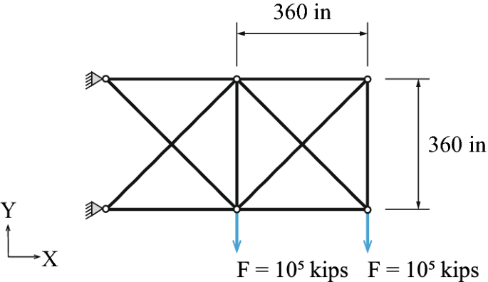

  

  10-bar truss system

These cases are selected to study the effect of topology optimization and displacement bounds on the computation time. As suggested by Bollapragada et al. (2001) and Van Mellaert (2017), discrete truss optimization problems may become significantly harder to solve in the presence of tight displacement constraints. Formulation variants (F^GG)*, (${\mathrm{F}}^{{\mathrm{BSF}}_{1}}$)*, and (${\mathrm{F}}^{{\mathrm{BSF}}_{2}}$)* (cf. Sect. 3.1) are only considered for cases (a), (b), and (c) where topology optimization is included. In the other cases (b), (d), and (f), no zero-area elements can be assigned and due to stress limits (i.e., strains), the elongation variables v_ij are always constrained by stress-based bounds rather than by displacement-based bounds (cf. Eqs. (47) and (48)).

Figure 12 shows the optimal topology and sizing for all cases (a)–(f). For cases (a) and (b), all formulations produce identical, globally optimal designs. In case (b), the solution has a weight of 1856.7 lb which is identical to that of the solution presented by Van Mellaert (2017). Solutions for cases (a), (c), and (d) are not available in the literature. As expected, including topology optimization produces structures with a lower weight compared to solutions obtained through sizing optimization carried out with a fixed topology. In cases (c) and (d), the formulations (F^GG), (${\mathrm{F}}^{{\mathrm{BSF}}_{1}}$), and (${\mathrm{F}}^{{\mathrm{BSF}}_{2}}$) and their variants are solved to global optimality within 3.4 – 417 s, whereas for (F^RS), it is not possible to obtain the global optimum within the set time limit of 5 h (cf. Table 4). For (F^RS), a MIP-gap > 0% remains at termination and the best upper-bound solution is reported. For this reason, the solution obtained by (F^RS) is different than that obtained by the other formulations, as shown in Fig. 12(c) and (d).

Fig. 12

10-bar truss results for cases a–f. For cases c and d, formulation (F^RS) produces different upper-bound solutions compared to the other formulations (cf. Table 4). The line thickness is proportional to the cross-section area indicated in [in²]

Generally, including topology optimization only marginally increases the problem size: only a zero-area element is added to the other 42 candidate cross sections (cf. cases (a) and (b), Table 4). Figure 13, 14, 15, 16, 17, and 18 show the convergence plots for cases (a) – (f), respectively. In cases (a) – (d), (${\mathrm{F}}^{{\mathrm{BSF}}_{1}}$)^(*) is the fastest to verify global optimality. The lower bounds obtained through (${\mathrm{F}}^{{\mathrm{BSF}}_{1}}$)* increase significantly faster than through the other formulations, thus, allowing the verification of global optimality in a shorter computation time. The lower bounds of (F^RS) practically stagnate in (c) and (d). For cases (e) and (f), in which the displacement bounds are tightened, none of the formulations can verify global optimality within the set time limit of 5 h. The lower bounds increase steeply early in the branch-and-bound process and stagnate after 5000 s. The remaining MIP-gap (distance between upper and lower bounds) at termination is the smallest for (${\mathrm{F}}^{{\mathrm{BSF}}_{1}}$)* and (${\mathrm{F}}^{{\mathrm{BSF}}_{1}}$) in cases (e) and (f), respectively. For cases (a) and (b) with large displacement bounds, topology optimization has practically no effect on computation time. Allowing topology optimization in case (c) produces solutions faster than in case (d) in which the topology is fixed. The problem size does not change when the displacement limits u^min and u^max are tighter. Only the elongation bounds and big-M constants change. Hence, it is clear that the computational performance is not only affected by the MILP problem size but also by numerical specificities. Generally, the formulations that employ member elongations as design (state) variables (F^GG, ${\mathrm{F}}^{{\mathrm{BSF}}_{1}}$, and ${\mathrm{F}}^{{\mathrm{BSF}}_{2}}$) are able to obtain better feasible solutions (upper bounds) in less time than (F^RS). This might be due to the direct correlation of member elongations and nodal displacements through geometric compatibility. The upper-bound solutions of 4962.1 and 5490.7 lb that have been obtained within a few seconds through (F^GG), (${\mathrm{F}}^{{\mathrm{BSF}}_{1}}$), and (${\mathrm{F}}^{{\mathrm{BSF}}_{2}}$) in cases (e) and (f) have the same quality as the best solutions reported in previous work in which solutions have been obtained through (meta-)heuristic algorithms (Camp et al. 2005; Juang et al. 2003; Kripka 2004; Rajan 1995; Schmid 1993; Sonmez 2011; Zhang et al. 2014). This shows that the MILP formulations are effective to produce high-quality solutions in a short computation time, even though global optimality might not be verified.

Fig. 13

Convergence plot 10-bar truss case (a)

Fig. 14

Convergence plot 10-bar truss case (b)

Fig. 15

Convergence plot 10-bar truss case (c)

Fig. 16

Convergence plot 10-bar truss case (d)

Fig. 17

Convergence plot 10-bar truss case (e)

Fig. 18

Convergence plot 10-bar truss case (f)

Table 4 10-bar truss results; bold values indicate the shortest computation time

3.4 Case study 4: 25-bar tower

The fourth case study is a “25-bar tower” that has been often studied in previous work (Rajeev and Krishnamoorthy 1992; Zhang et al. 2014). Dimensions, support locations, and loading are indicated in Fig. 19. The tower members are divided into eight groups as indicated in Table 5. The labels “S-E” refer to the start and end node of each member. Node numbering is shown in Fig. 19. The structural elements’ material is assumed to have Young’s modulus of 10⁷ psi and yield strength of 40 × 10³ psi. Weight minimization is carried out by factoring the structure volume (Eq. (2)) with a material density of 0.1 lb/in³. The set of 30 candidate cross-section areas comprises a = {0.1, 0.2, 0.3, 0.4, 0.5, 0.6, 0.7, 0.8, 0.9, 1.0, 1.1, 1.2, 1.3, 1.4, 1.5, 1.6, 1.7, 1.8, 1.9, 2.0, 2.1, 2.2, 2.3, 2.4, 2.5, 2.6, 2.8, 3.0, 3.2, 3.4} in² (Rajeev and Krishnamoorthy 1992). For all members within a group, the same cross section is assigned. Two cases are investigated:

• Case (a): the X- and Y-displacements of Nodes 1 and 2 are limited to ± 1.0 in, the Z-displacements to ± 50.0 in

• Case (b): the X- and Y-displacements of Nodes 1 and 2 are limited to ± 0.35 in, the Z-displacements to ± 50.0 in

  Fig. 19

  

  25-bar tower truss

Table 5 Member grouping 25-bar tower truss

For all other nodes, the X-, Y-, and Z-displacements are limited to ± 50.0 in. The structure topology is kept constant and only cross-section sizing is performed. These cases are considered to study the effect of reducing the displacement bounds on computational performance for a more complex configuration (3D) compared to previous cases. Formulation variants (F^GG)*, (${\mathrm{F}}^{{\mathrm{BSF}}_{1}}$)*, and (${\mathrm{F}}^{{\mathrm{BSF}}_{2}}$)* (cf. Sect. 3.1) are not considered for this case study because the topology is invariant and the elongation variables v_ij are constrained by stress- and not by displacement-based bounds (cf. Eqs. (47) and (48)).

Table 6 gives the optimization problem size for all four formulations. The problem size is identical for both cases (a) and (b) as only the displacement bounds are changed. Table 7 gives optimization metrics for the branch-and-bound process and Table 8 indicates the optimal cross sections assigned to each member group.

Table 6 Optimization problem sizes

Table 7 5-bar tower truss results; bold values indicate the shortest computation time

Table 8 Member group optimal cross-section areas

Figures 20 and 21 show the convergence plots of the four formulations for cases (a) and (b), respectively. As in previous sections, formulations (F^GG), (${\mathrm{F}}^{{\mathrm{BSF}}_{1}}$), and (${\mathrm{F}}^{{\mathrm{BSF}}_{2}}$) obtain faster increasing lower bounds. In case (a), (F^RS) is significantly slower compared to the other formulations to verify solution global optimality. In case (b), the global optimum with a weight of 484.3 lb. has been obtained by all formulations. (${\mathrm{F}}^{{\mathrm{BSF}}_{2}}$) obtains the optimal solution and verifies global optimality in the shortest computation time. Remarkably, (${\mathrm{F}}^{{\mathrm{BSF}}_{2}}$) reaches the optimal upper bound after 219 s whereas it takes the other formulations 1 – 5 h. In case (b), global optimality cannot be verified through (F^RS) within the set time limit of 5 h (remaining MIP-gap = 58%). The globally optimal design in (b) is identical to the best solution obtained through meta-heuristics in the literature (Zhang et al. 2014). To the authors' knowledge, it is the first time that solution global optimality for this 25-bar tower truss design is verified through a deterministic method (MILP).

Fig. 20

Convergence plot case (a): u_xy ≤  ± 1.0 in

Fig. 21

Convergence plot case (b): u_xy ≤  ± 0.35 in

4 Discussion

4.1 MILP formulation performance

Different MILP formulations (F^RS), (F^GG), (${\mathrm{F}}^{{\mathrm{BSF}}_{1}}$), and (${\mathrm{F}}^{{\mathrm{BSF}}_{2}}$) for discrete sizing and topology optimization of truss structures are benchmarked in Sect. 3. The benchmark studies have shown that, generally, a slightly larger number of variables, constraints, and non-zeros entries in the constraint matrix may not necessarily result in a significantly longer computation time. This is the case for formulations (F^GG), (${\mathrm{F}}^{{\mathrm{BSF}}_{1}}$), and (${\mathrm{F}}^{{\mathrm{BSF}}_{2}}$). Differently, formulation (F^RS) involves a significantly larger number of variables, constraints, and non-zero entries in the constraint matrix (Sect. 2.5) which requires exploring more nodes of the search tree and thus solving more LP relaxations. In addition, the LP relaxations are harder to solve because they require more Simplex iterations due to the higher number of variables and constraints. For these reasons, (F^RS) requires a significantly longer computation time to reach the optimal solution (upper bound) and verify global optimality compared to the other three formulations.

It is more challenging to assess how the mathematical structure of a formulation affects computational performance. In the attempt to reach a holistic understanding of the performance of the MILP formulations, a synthesis of the case studies discussed in (Sects. 3.1 – 3.4) is offered in this section by focusing on three benchmark metrics ${m}^{k \in \{\mathrm{1,2},3\}}$: ${m}^{1}$ total computation time to verify global optimality, ${m}^{2}$ the number of nodes explored in the search tree, and ${m}^{3}$ the computation time required to obtain upper-bound solutions that are global optima (although global optimality has not been verified).

The formulations are evaluated by ranking their performance for all cases and through performance profiles (Dolan and Moré 2002). Performance profiles have been employed to benchmark the performance of optimization solvers for topology optimization problems by Rojas-Labanda and Stolpe (2015) among others.

In this work, performance profiles are employed to evaluate the performance of different MILP formulations to solve volume minimization through discrete sizing and topology optimization. Since the problem is identical and all case studies are carried out using the same optimization solver, the focus of the assessment is on the performance of the mathematical formulation of the problem.

The performance profiles are built for each metric of interest ${m}_{c,f}^{k}$ and for each formulation$f\in \mathcal{F}=\{1, 2 ,... 7\}$, including the (F)* variants, to solve problem cases $c\in \mathcal{C}=\{1, 2 .. {n}_{c}\}$. The ratio of performance ${r}_{c,f}^{k}$ compares the performance of a formulation against the best performance among all formulations for a specific case:

$${r}_{c,f}^{k}= \frac{{m}_{c,f}^{k}}{\mathrm{min}\{{m}_{c,f}^{k}:f\in \mathcal{F}\}}.$$

(63)

When ${r}_{c,f}^{k}=1$, formulation $f$ performs best for case study $c$ with respect to metric ${m}^{k}$, otherwise ${r}_{c,f}^{k}$ quantifies formulation $f$ performance ratio with respect to the best performing formulation (Dolan and Moré 2002). The performance of a formulation $f$ with respect to metric ${m}^{k}$ is defined as the probability that the performance ratio ${r}_{c,f}^{k}$ is at most a factor τ to the best performance ratio:

$${\rho }_{f}^{k}\left(\tau \right)= \frac{1}{{n}_{c}}\text{size}\{c\in \mathcal{C}:{r}_{c,f}^{k}\le\uptau \}$$

(64)

In other words, ${\rho }_{f}^{k}\left(\tau \right)$ is the probability that, in the worst case, formulation $f$ performance is lower by a factor τ compared to the best performing formulation (Dolan and Moré 2002). ${n}_{c}$ denotes the total number of problem cases. Table 9 gives the formulation ranking with respect to ${m}^{1}$ for all ${n}_{c}$ = 10 cases where global solution optimality has been proven (i.e., all cases except (e) and (f) in Sect. 3.3). The figures indicate in how many cases a formulation $f$ has performed at a certain rank. Figure 22 gives the corresponding performance profile. Generally, it is desirable to observe a significant performance increase for small variations of τ. When a performance profile grows fast as τ increases, it indicates that the corresponding formulation performs close to the best one over the entire test set. (F^GG) has 90% probability to perform with a ratio of at most 1.8 times the computation time of the fastest formulation. (${\mathrm{F}}^{{\mathrm{BSF}}_{1}}$)* has the highest probability to perform with a ratio of 1.5 (70%) and 1.0 (30%). Adding the displacement-based elongation bounds (big-M constants) brings no significant improvement in (F^GG)*. Removing the displacement-based elongation bounds is beneficial to (${\mathrm{F}}^{{\mathrm{BSF}}_{1}}$)* and (${\mathrm{F}}^{{\mathrm{BSF}}_{2}}$)* as their performance grows faster for small values of τ ≤ 3.

Table 9 Ranking (${m}^{1})$ with respect to the computation time required to verify global optimality

Fig. 22

Performance profile ${\rho }_{f}^{1}$, computation time to verify global optimality

Generally, formulations (F^GG), (${\mathrm{F}}^{{\mathrm{BSF}}_{1}}$), and (${\mathrm{F}}^{{\mathrm{BSF}}_{2}}$) perform well for strength-governed problems. As mentioned in (Bollapragada et al. 2001; Van Mellaert 2017) and shown in Sects. 3.3 and 3.4, displacement bounds can strongly influence computational performance. Formulations (F^GG), (${\mathrm{F}}^{{\mathrm{BSF}}_{1}}$), and (${\mathrm{F}}^{{\mathrm{BSF}}_{2}}$) require significantly reduced computation time compared to (F^RS) when moderate displacement bounds are set. However, when displacement constraints are tight, resulting in low utilization of element capacity (i.e., stiffness-governed problems), it becomes difficult to verify global optimality, regardless of the formulation (cases (e) and (f), Sect. 3.3). In those cases where global optimality has not been verified within the time limit, employing (${\mathrm{F}}^{{\mathrm{BSF}}_{1}}$) has resulted in the smallest MIP-gaps, i.e., it provides the tightest lower bounds. Table 10 gives the formulation ranking with respect to ${m}^{2}$, the number of explored search tree nodes. It is clear that (${\mathrm{F}}^{{\mathrm{BSF}}_{1}}$) requires by far the least number of continuous LP relaxations to be solved. This indicates the efficiency of (${\mathrm{F}}^{{\mathrm{BSF}}_{1}}$) to provide fast increasing lower bounds. In general, solving LP relaxations of different search tree nodes can be carried out independently on different computing cores (Gendron and Crainic 1994), which might further improve the performance of (${\mathrm{F}}^{{\mathrm{BSF}}_{1}}$) when the number of CPU cores is increased. Figure 23 gives the corresponding performance profile. In this case, only the variants (F^GG)* and (${\mathrm{F}}^{{\mathrm{BSF}}_{2}}$)* perform slightly better than the corresponding original formulations.

Table 10 Ranking (${m}^{2})$ with respect to the number of explored search tree nodes

Fig. 23

Performance profile ${\rho }_{f}^{2}$, number of explored search tree nodes

In all cases, it has been observed that (near-)optimal integer-feasible solutions (upper bounds) are obtained very early in the branch-and-bound process and that most of the total computation time is spent to verify global optimality through increasing lower bounds. Table 11 gives the formulation ranking with respect to ${m}^{3}$ and Fig. 24 the corresponding performance profile. In most cases, (F^RS) has the worst performance. In this case, the addition of displacement-based elongation bounds (big-M constants) improves (F^GG)* performance significantly, which is the fastest to obtain high-quality upper-bound solutions in 60% of all cases (τ = 1). Adding the displacement-based elongation bounds halves the performance ratio reducing it to 2.0 from 4.3 for a probability of 90%. On the contrary, removing the displacement-based elongation bounds is beneficial to the performance of (${\mathrm{F}}^{{\mathrm{BSF}}_{2}}$)*.

Table 11 Ranking (m³) with respect to the computation time required to reach upper-bound solutions that are global optima (global optimum not yet verified)

Fig. 24

Performance profile ${\rho }_{f}^{3}$, computation time to reach upper-bound solutions that are global optima

In general, this analysis confirms that the MILP formulations investigated in this work are effective to produce high-quality solutions in a short computation time. The study of the variants (F)* has shown that when the difference in the number of variables and constraints is small, the mathematical structure of the problem has a significant influence on the formulation performance.

Over the last few years, the performance of MILP solvers has improved significantly due to advances in method implementation and increased computing power. This is evident when comparing the computation times reported in this work with those given in the literature (cf. case studies 1 and 2 in Sects. 3.1 and 3.2 with those reported by Rasmussen and Stolpe (2008)). To the authors' knowledge, it is the first time that solution global optimality has been verified for the 25-bar tower truss design (Sect. 3.4).

From the cases studied in this paper, it can be inferred that (F^GG), (${\mathrm{F}}^{{\mathrm{BSF}}_{1}}$), and (${\mathrm{F}}^{{\mathrm{BSF}}_{2}}$) will perform better for larger-scale problems compared to (F^RS). (${\mathrm{F}}^{{\mathrm{BSF}}_{1}}$) (and its variant) has the highest probability to verify global optimality in the shortest computation time. Nevertheless, solving MILP to global optimality with branch-and-bound methods is at worst-case exponentially complex, which might limit the application of the presented formulations to small- to medium-scale problems (< 200 structural members and < 50 candidate cross-section areas).

4.2 Limitations and future work

This work offers a benchmark of a new MILP-based formulation for sizing and topology optimization of truss structures against two well-known formulations. The benchmark is based on four problem cases (although with sub-cases to evaluate the influence of displacement constraints) of small and medium sizes. Future studies could deepen the generalization of the conclusions reached in this work by extending the benchmark to other problems. The purpose of the benchmark given in this work is to investigate the specificities of discrete sizing and topology optimization subject to stress and displacement limits and without the influence of additional constraints such as global stability (including mechanism avoidance), member overlapping, and buckling. In addition, such constraints are not included in the benchmark formulations. Other formulations that include constraints on global stability, member overlapping, or member buckling have been developed (Fairclough and Gilbert 2020; Mela 2014; Ohsaki and Katoh 2005). Future work could extend the formulation given in this paper by implementing such constraints and investigating their influence on computational performance and solution quality.

Solving MILPs through branch-and-bound algorithms can be parallelized to multiple computing cores (Bertsimas and Tsitsiklis 1997; Gendron and Crainic 1994; Gurobi Optimization, LLC 2019). Although computation time might not reduce significantly for large-scale problems owing to the exponential complexity of MILP (Nemhauser and Wolsey 1999), future work could look into evaluating the potential improvement margin through parallelization that depends on the formulation type. The examples analyzed in this work have shown that verifying global optimality is harder than obtaining optimal or near-optimal upper-bound solutions, especially when displacements are limited by tight bounds. Future work could (1) study the correlation between the MILP mathematical model and the effect of tight displacement bounds, (2) quantify further the formulation performances through additional studies, and (3) develop formulations that enable tighter lower bounds to reduce the MIP-gap faster. The latter might be achieved by adding other sets of redundant design and state variables as well as redundant constraints. Another approach that might lead to improvement could be that proposed by (Shahabsafa et al. 2018) who developed an incremental assignment formulation for discrete cross sections, which has shown to reduce computation time. It has been observed that certain settings of the Gurobi solver (Gurobi Optimization, LLC 2019) employed in this work may affect computational performance. In this work, most of the solver parameters have been kept at the default value. Future work could carry out parameter tuning to improve computational performance and benchmark results with other software (e.g., CPLEX (IBM 2020)).

5 Conclusion

This work has introduced a new MILP-based formulation for sizing and topology optimization of truss structures. A benchmark study with two well-known existing formulations has shown that the computation time to obtain global optima via a branch-and-bound solver highly depends on the chosen set of variables and constraints. The benchmark given in this paper, which is the first of this kind, has helped to gain a deeper insight on how to improve MILP formulations. Through appropriate formulation variations, it is possible to significantly improve computational performance. One of the existing formulations (F^RS) performs significantly worse compared to all other formulations. Instead, formulations that employ member elongations as state variables (F^GG, ${\mathrm{F}}^{{\mathrm{BSF}}_{1}}$, and ${\mathrm{F}}^{{\mathrm{BSF}}_{2}}$) are able to obtain near-optimal upper bounds and global optima much faster. The formulation (F^GG), previously developed by Ghattas and Grossmann (1991), has been improved by adding displacement-based elongation bounds (big-M constants), which enables obtaining high-quality upper-bound solutions in a very short computation time. The new formulation (${\mathrm{F}}^{{\mathrm{BSF}}_{1}}$) is, generally, faster to verify global optimality and also requires exploring significantly fewer nodes in the search tree.

References

Arora JS, Wang Q (2005) Review of formulations for structural and mechanical system optimization. Struct Multidisc Optim 30:251–272. https://doi.org/10.1007/s00158-004-0509-6
Bennage WA, Dhingra AK (1995) Single and multiobjective structural optimization in discrete-continuous variables using simulated annealing. Int J Numer Methods Eng 38:2753–2773. https://doi.org/10.1002/nme.1620381606
Bertsimas D, Tsitsiklis JN (1997) Introduction to linear optimization. Athena Scientific, Belmont
Bollapragada S, Ghattas O, Hooker JN (2001) Optimal design of truss structures by logic-based branch and cut. Oper Res 49:42–51. https://doi.org/10.1287/opre.49.1.42.11196
Brütting J, Desruelle J, Senatore G, Fivet C (2019) Design of truss structures through reuse. Structures 18:128–137. https://doi.org/10.1016/j.istruc.2018.11.006
Brütting J, Vandervaeren C, Senatore G, De Temmerman N, Fivet C (2020) Environmental impact minimization of reticular structures made of reused and new elements through Life Cycle Assessment and Mixed-Integer Linear Programming. Energy Build 215:109827. https://doi.org/10.1016/j.enbuild.2020.109827
Camp CV, Bichon BJ, Stovall SP (2005) Design of steel frames using ant colony optimization. J Struct Eng 131:369–379. https://doi.org/10.1061/(ASCE)0733-9445(2005)131:3(369)
Deb K, Gulati S (2001) Design of truss-structures for minimum weight using genetic algorithms. Finite Elem Des 37:447–465. https://doi.org/10.1016/S0168-874X(00)00057-3
Dolan ED, Moré JJ (2002) Benchmarking optimization software with performance profiles. Math Program 91:201–213. https://doi.org/10.1007/s101070100263
Dorn WS, Gomory RE, Greenberg HJ (1964) Automatic design of optimal structures. J Mec 3:25–52
Fairclough H, Gilbert M (2020) Layout optimization of simplified trusses using mixed integer linear programming with runtime generation of constraints. Struct Multidisc Optim 61:1977–1999. https://doi.org/10.1007/s00158-019-02449-7
Gendron B, Crainic TG (1994) Parallel Branch-and-Branch Algorithms: Survey and Synthesis. Oper Res. https://doi.org/10.1287/opre.42.6.1042
Ghattas, O.N., Grossmann, I.E., 1991. MINLP and MILP Strategies for Discrete Sizing Structural Optimization Problems. Electron. Comput. 197–204.
Gilbert M, Tyas A (2003) Layout optimization of large-scale pin-jointed frames. Eng Comput 20:1044–1064. https://doi.org/10.1108/02644400310503017
Glover F (1975) Improved linear integer programming formulations of nonlinear integer problems. Manag Sci 22:455–460. https://doi.org/10.1287/mnsc.22.4.455
Glover F (1984) An improved MIP formulation for products of discrete and continuous variables. J Inf Optim Sci 5:69–71
Gurobi Optimization, LLC (2019) Gurobi optimizer reference manual. Gurobi Optimization, LLC, Houston
Haftka RT (1985) Simultaneous analysis and design. AIAA J 23:1099–1103
Huang M-W, Arora JS (1997) Optimal design of steel structures using standard sections. Struct Optim 14:24–35. https://doi.org/10.1007/BF01197555
IBM (2020) CPLEX optimizer
Juang D-S, Wu Y-T, Chang W-T (2003) Optimum design of truss structures using discrete Lagrangian method. J Chin Inst Eng 26:635–646. https://doi.org/10.1080/02533839.2003.9670817
Kaveh A, Kalatjari V (2002) Genetic algorithm for discrete-sizing optimal design of trusses using the force method. Int J Numer Methods Eng 55:55–72. https://doi.org/10.1002/nme.483
Kripka M (2004) Discrete optimization of trusses by simulated annealing. J Braz Soc Mech Sci Eng 26:170–173
Lagaros ND (2018) The environmental and economic impact of structural optimization. Struct Multidisc Optim 58:1751–1768. https://doi.org/10.1007/s00158-018-1998-z
Li LJ, Huang ZB, Liu F (2009) A heuristic particle swarm optimization method for truss structures with discrete variables. Comput Struct 87:435–443. https://doi.org/10.1016/j.compstruc.2009.01.004
Mela K (2014) Resolving issues with member buckling in truss topology optimization using a mixed variable approach. Struct Multidisc Optim 50:1037–1049. https://doi.org/10.1007/s00158-014-1095-x
Van Mellaert R (2017) Optimal design of steel structures according to the Eurocodes using mixed-integer linear programming methods. PhD thesis. KU Leuven, Leuven, Belgium
Nemhauser GL, Wolsey LA (1999) Integer and combinatorial optimization. Wiley, New York
Ohsaki M (2017) Optimization of finite dimensional structures, 1st edn. Routledge, Boca Raton
Ohsaki M, Katoh N (2005) Topology optimization of trusses with stress and local constraints on nodal stability and member intersection. Struct Multidisc Optim 29:190–197. https://doi.org/10.1007/s00158-004-0480-2
Pellens J, Lombaert G, Lazarov B, Schevenels M (2019) Combined length scale and overhang angle control in minimum compliance topology optimization for additive manufacturing. Struct Multidisc Optim 59:2005–2022. https://doi.org/10.1007/s00158-018-2168-z
Rajan SD (1995) Sizing, shape, and topology design optimization of trusses using genetic algorithm. J Struct Eng 121:1480–1487. https://doi.org/10.1061/(ASCE)0733-9445(1995)121:10(1480)
Rajeev S, Krishnamoorthy CS (1992) Discrete optimization of structures using genetic algorithms. J Struct Eng 118:1233–1250. https://doi.org/10.1061/(ASCE)0733-9445(1992)118:5(1233)
Rasmussen MH, Stolpe M (2008) Global optimization of discrete truss topology design problems using a parallel cut-and-branch method. Comput Struct 86:1527–1538. https://doi.org/10.1016/j.compstruc.2007.05.019
Rojas-Labanda S, Stolpe M (2015) Benchmarking optimization solvers for structural topology optimization. Struct Multidisc Optim 52:527–547. https://doi.org/10.1007/s00158-015-1250-z
Rozvany GIN, Bendsoe MP, Kirsch U (1995) Layout optimization of structures. Appl Mech Rev 48:41–119. https://doi.org/10.1115/1.3005097
Schmid L (1993) Discussion of "Discrete Optimization of Structures Using Genetic Algorithms” by S. Rajeev and C. S. Krishnamoorthy (May, 1992, Vol. 118, No. 5). J Struct Eng 119:2494–2495. https://doi.org/10.1061/(ASCE)0733-9445(1993)119:8(2494)
Shahabsafa M, Mohammad-Nezhad A, Terlaky T, Zuluaga L, He S, Hwang JT, Martins JRRA (2018) A novel approach to discrete truss design problems using mixed integer neighborhood search. Struct Multidisc Optim 58:2411–2429. https://doi.org/10.1007/s00158-018-2099-8
Shea K, Smith IFC (2006) Improving full-scale transmission tower design through topology and shape optimization. J Struct Eng 132:781–790. https://doi.org/10.1061/(ASCE)0733-9445(2006)132:5(781)
Smith CJ, Gilbert M, Todd I, Derguti F (2016) Application of layout optimization to the design of additively manufactured metallic components. Struct Multidisc Optim 54:1297–1313. https://doi.org/10.1007/s00158-016-1426-1
Sonmez M (2011) Discrete optimum design of truss structures using artificial bee colony algorithm. Struct Multidisc Optim 43:85–97. https://doi.org/10.1007/s00158-010-0551-5
Stolpe M (2016) Truss optimization with discrete design variables: a critical review. Struct Multidisc Optim 53:349–374. https://doi.org/10.1007/s00158-015-1333-x
Stolpe M, Svanberg K (2003) Modelling topology optimization problems as linear mixed 0–1 programs. Int J Numer Methods Eng 57:723–739. https://doi.org/10.1002/nme.700
Toakley AR (1968) Optimum design using available sections. J Struct Div 94:1219–1244
Van Mellaert R, Lombaert G, Schevenels M (2016) Global size optimization of statically determinate trusses considering displacement, member, and joint constraints. J Struct Eng 142:04015120. https://doi.org/10.1061/(ASCE)ST.1943-541X.0001377
Venkayya VB (1971) Design of optimum structures. Comput Struct 1:265–309. https://doi.org/10.1016/0045-7949(71)90013-7
Zhang Y, Hou Y, Liu S (2014) A new method of discrete optimization for cross-section selection of truss structures. Eng Optim 46:1052–1073. https://doi.org/10.1080/0305215X.2013.827671
Funding
Open access funding provided by EPFL Lausanne. This research received no specific grant from any funding agency in the public, commercial, or not-for-profit sectors.
Author information
Authors and Affiliations
Corresponding author
Ethics declarations
Conflict of interest
The authors declare that there is no conflict of interest.
Replication of results
All formulation and case study details required for replication of results have been reported in the article. In addition, MILP model files (.mps format) for all case studies are provided as supplementary data. These files can be executed with Gurobi and other commercial MILP solvers. The employed Gurobi-C# implementation will be made available by the authors upon request.
Additional information
Responsible Editor: Mathias Stolpe
Publisher's Note
Springer Nature remains neutral with regard to jurisdictional claims in published maps and institutional affiliations.
Supplementary Information
Below is the link to the electronic supplementary material.
Rights and permissions
Open Access This article is licensed under a Creative Commons Attribution 4.0 International License, which permits use, sharing, adaptation, distribution and reproduction in any medium or format, as long as you give appropriate credit to the original author(s) and the source, provide a link to the Creative Commons licence, and indicate if changes were made. The images or other third party material in this article are included in the article's Creative Commons licence, unless indicated otherwise in a credit line to the material. If material is not included in the article's Creative Commons licence and your intended use is not permitted by statutory regulation or exceeds the permitted use, you will need to obtain permission directly from the copyright holder. To view a copy of this licence, visit http://creativecommons.org/licenses/by/4.0/.
About this article
Cite this article
Brütting, J., Senatore, G. & Fivet, C. MILP-based discrete sizing and topology optimization of truss structures: new formulation and benchmarking. Struct Multidisc Optim 65, 277 (2022). https://doi.org/10.1007/s00158-022-03325-7
Received:
Revised:
Accepted:
Published:
DOI: https://doi.org/10.1007/s00158-022-03325-7