Fully Secure Functional Encryption with a Large Class of Relations from the Decisional Linear Assumption

Abstract

This paper presents a fully secure (adaptively secure) practical functional encryption scheme for a large class of relations, that are specified by non-monotone access structures combined with inner-product relations. The security is proven under a standard assumption, the decisional linear assumption, in the standard model. Our scheme is constructed on the concept of dual pairing vector spaces and a hierarchical reduction technique on this concept is employed for the security proof. The proposed functional encryption scheme covers, as special cases, (1) key-policy, ciphertext-policy and unified-policy attribute-based encryption with non-monotone access structures, (2) (hierarchical) attribute-hiding functional encryption with inner-product relations and functional encryption with nonzero inner-product relations and (3) spatial encryption and a more general class of encryption than spatial encryption.

1 Introduction

1.1 Background

Although numerous encryption systems have been developed over several thousand years, any traditional encryption system before the 1970’s had a great restriction on the relation between a ciphertext encrypted by an encryption key and the decryption key such that these keys should be equivalent. The innovative notion of public key cryptosystems in the 1970’s relaxed this restriction, where these keys differ and the encryption key can be published, but the decryption key is firmly related to the encryption key for the unique decryption of a ciphertext to its plaintext.

Recently, a new innovative class of encryption systems, functional encryption (FE), has been introduced [14, 15, 28, 41, 44], where a secret (decryption) key, ${\textsf {sk}}_{f}$, is associated with a function f, an input x (to f) is encrypted to a ciphertext ${\textsf {Enc}}({\textsf {pk}},x)$ using system (master) public key ${\textsf {pk}}$, and the ciphertext is decrypted by the secret to f(x).

This notion provides more sophisticated and flexible relations between decryption keys and ciphertexts such that a secret key, ${\textsf {sk}}_{\Psi }$, is associated with a parameter, $\Psi$, and message m is encrypted to a ciphertext ${\textsf {Enc}}({\textsf {pk}}, (m,\Upsilon ))$ using system public key ${\textsf {pk}}$ along with another parameter $\Upsilon$. Ciphertext ${\textsf {Enc}}({\textsf {pk}},(m,\Upsilon ))$ can be decrypted by secret ${\textsf {sk}}_{\Psi }$ if and only if a relation (predicate) $R(\Psi ,\Upsilon )$ holds. Here, $x := (m,\Upsilon )$ is an input to encryption of FE and the function $f_{R, \Psi }$ (with secret key ${\textsf {sk}}_{\Psi }$) of $x:= (m,\Upsilon )$ is m if and only if a relation $R(\Psi ,\Upsilon )$ holds. Such a concept of FE has various applications in the areas of access control for databases, mail services, and contents distribution [5, 12, 15, 28, 30, 42,43,44,45, 48].

When R is the simplest relation or equality relation, i.e., $R(\Psi ,\Upsilon )$ holds iff $\Psi =\Upsilon$, it is identity-based encryption (IBE) [6,7,8, 10, 16, 21, 24, 25].

As a more general class of FE, attribute-based encryption (ABE) schemes have been proposed [5, 12, 15, 28, 30, 42,43,44,45, 48], where either one of the parameters for encryption and secret key is a tuple of attributes, and the other is a policy on attributes. Here each attribute is an element of a finite field or ring. For example, a policy ${\Psi }$ is an access structure ${\hat{M}}$ along with a tuple of attributes $(v_1,\ldots ,v_\iota )$ for a secret key, and a tuple of attributes, $\Upsilon := (x_1,\ldots ,x_\iota )$, for encryption. Here, some elements of the tuples may be empty. $R(\Psi ,\Upsilon )$ holds iff the truth-value vector of $({\textsf {T}}(x_1 = v_1),\ldots ,{\textsf {T}}(x_\iota = v_\iota ))$ is accepted by ${\hat{M}}$, where ${\textsf {T}}(\cdot )$ is a predicate such that ${\textsf {T}}(\psi ) := 1$ if $\psi$ is true, and ${\textsf {T}}(\psi ) := 0$ if $\psi$ is false (For example, ${\textsf {T}}(x = v) := 1$ if $x = v$, and ${\textsf {T}}(x = v) := 0$ if $x \not = v$). A monotone general access structure can express any monotone formula over atomic terms of ${\textsf {T}}(x_1 = v_1),\ldots ,{\textsf {T}}(x_\iota = v_\iota )$. If parameter $\Psi$ for a secret key is an access structure (policy), it is called key-policy ABE (KP-ABE). If parameter $\Upsilon$ for encryption is a policy, it is ciphertext-policy ABE (CP-ABE).

Inner-product predicate encryption (IPE) [30] is a class of FE for inner-product relations (predicates), where each parameter for encryption and secret key is a vector over a field or ring (e.g., $\vec {x} := (x_1,\ldots ,x_n) \in {\mathbb {F}}_q^{\,n}$ and $\vec {v} := (v_1,\ldots ,v_n) \in {\mathbb {F}}_q^{\,n}$ for encryption and secret key, respectively), and $R(\vec {v},\vec {x})$ holds iff $\vec {x} \cdot \vec {v} = 0$, where $\vec {x} \cdot \vec {v}$ is the inner-product of $\vec {x}$ and $\vec {v}$. The inner-product relation represents a wide class of relations including equality, conjunction and disjunction (more generally, CNF and DNF) of equality relations and polynomial relations.

There are two types of secrecy on ciphertexts in FE, attribute-hiding (private-index) and payload-hiding (public-index) [30]. Roughly speaking, attribute-hiding requires that a ciphertext conceal the associated parameter as well as the plaintext, while payload-hiding only requires that a ciphertext conceal the plaintext. Anonymous IBE and hidden-vector encryption (HVE) [15] are a special class of attribute-hiding IPE.

Although many practical FE schemes such as ABE and IPE schemes have been presented over the last decade, existing fully secure (adaptively secure) practical FE schemes only support some restricted classes of relations, e.g., monotone access structures with equality relations, and inner-product relations.

1.2 Our Result

In this paper, we propose fully secure practical FE schemes that supports more general relations than monotone access structures with equality relations and inner-product relations. Our scheme is secure in the standard assumption, the decisional linear (DLIN) assumption (over any type of prime-order bilinear groups), in the standard model.

More precisely, this paper presents a fully secure (adaptively secure against CPA) practical FE scheme for a large class of relations, that are specified by non-monotone access structures combined with inner-product relations. Similarly to the existing ABE schemes, we propose three types of FE schemes, the KP-FE and CP-FE schemes (in Sects. 4, 5) as well as a generalized notion of KP-FE and CP-FE, unified-policy FE (UP-FE).¹ (in Sect. 6).

In our KP-FE scheme, parameter $\Upsilon$ for a ciphertext is a tuple of (attribute) vectors and parameter $\Psi$ for a secret key is a non-monotone access structure or span program ${\hat{M}} := (M, \rho )$ along with a tuple of vectors, e.g., $\Upsilon := (\vec {x}_1,\ldots ,\vec {x}_\iota ) \in {\mathbb {F}}_q^{\,n_1 + \cdots + n_\iota }$, and $\Psi := ({\hat{M}}, (\vec {v}_1,\ldots ,\vec {v}_\iota ) \in {\mathbb {F}}_q^{\,n_1 + \cdots + n_\iota })$. The component-wise inner-product relations for attribute vector components, e.g., $\{\vec {x}_t \cdot \vec {v}_t = 0$ or not $\}_{t\in \{1,\ldots ,\iota \}}$, are input to (non-monotone/monotone) span program ${\hat{M}}$, and $R(\Psi ,\Upsilon )$ holds iff the truth-value vector of $({\textsf {T}}(\vec {x}_1 \cdot \vec {v}_1 = 0), \ldots ,\mathsf{T}(\vec {x}_\iota \cdot \vec {v}_\iota = 0))$ is accepted by span program ${\hat{M}}$.

The proposed FE scheme is practical. For example, if the proposed FE scheme is specialized to IPE, the ciphertext size of our IPE scheme (“Appendix F.2”) is $(3n+2)\cdot |{\mathbb {G}}|$, whose information theoretical lower bound is $n \cdot |{\mathbb {F}}_q|$ if the vector elements are from ${\mathbb {F}}_q$. Here, n is the dimension of the attribute vectors, and $|{\mathbb {G}}|$ and $|{\mathbb {F}}_q|$ denote the sizes of an element of prime order pairing group ${\mathbb {G}}$ (for ciphertexts) and finite field ${\mathbb {F}}_q$, respectively, e.g., both are 256 bits. Then, the ciphertext size of our IPE scheme is just around three times longer than the theoretical lower bound.

It is easy to convert the (CPA-secure) proposed FE scheme to a CCA-secure FE scheme by employing an existing general conversion such as that by Canetti et al. [17] or that by Boneh and Katz [13] (using additional seven-dimensional dual spaces $({{\mathbb {B}}}_{d+1}, {{\mathbb {B}}}^{*}_{d+1})$ with $n_{d+1} := 2$ on the proposed FE scheme, and a strongly unforgeable one-time signature scheme or message authentication code with encapsulation) (see Sect. 7).

Since the proposed FE scheme supports a large class of relations, it includes the following schemes as special cases:

• 1. The (KP, CP and UP)-ABE schemes for non-monotone access structures with equality relations. Here, the underlying vectors of our FE scheme, $\{\vec {x}_t\}_{t\in \{1,\ldots ,d\}}$ and $\{\vec {v}_t\}_{t\in \{1,\ldots ,d\}}$, are specialized to two-dimensional vectors for the equality relation, e.g., $\vec {x}_t := (1,x_t)$ and $\vec {v}_t := (v_t,-1)$, where $\vec {x}_t\cdot \vec {v}_t=0$ iff $x_t = v_t$ (see “Appendix F.1” for KP-ABE).

  In these ABE schemes, attribute $x_t$ is expressed by the form of $(t,x_t)$ in place of just attribute $x_t$. Here, t identifies a subuniverse or category of attributes, and $x_t$ is an attribute in subuniverse t (examples of $(t,x_t)$ are (Name, Alice) and (Affiliation, Institute X)). The number of subuniverses, d, is a polynomial of security parameter $\lambda$, and the number of attributes in a subuniverse is exponential in $\lambda$.

• 2. The (zero-)IPE and nonzero-IPE schemes, where a nonzero-IPE scheme is a class of FE with $R(\vec {v},\vec {x})$ iff $\vec {x} \cdot \vec {v} \not = 0$. Here, the underlying access structure ${{\mathbb {S}}}$ of our FE scheme is specialized to the 1-out-of-1 secret sharing.

  See “Appendix F.2” for our IPE scheme, which is slightly modified from a straightforward IPE-specialization of our FE scheme for improving efficiency. Note that the IPE scheme is ‘weakly attribute-hiding,’ where a type of key queries are not allowed in ‘weakly attribute-hiding’ (see the definition in [32]). It is easy to modify this IPE scheme to a ‘fully attribute-hiding ([30])’ scheme by simply expanding the dimension of the space [38], while its security proof is quite different from that shown in “Appendix F.2” (see [38] for the security proof of fully attribute-hiding).

• 3. If the underlying access structure is specialized to the d-out-of-d secret sharing (conjunction formula), our FE scheme can be specialized to a hierarchical zero/nonzero-IPE scheme by adding delegation and re-randomization mechanisms. We show two hierarchical (zero-)IPE (HIPE) schemes in “Appendix G”, where one is payload-hiding and the other (weakly) attribute-hiding.

• 4. If the underlying access structure is a monotone formula with n-dimensional vectors, our FE scheme can be specialized to spatial encryption (for n-dimensional spaces) [12, 19].

  Here, we give some simple examples.

  • Let A be a s-dimensional subspace in the n-dimensional vector space V ($0< s < n$), which can be characterized by $(n-s)$ independent vectors in V, ($\vec {v}_1,.., \vec {v}_{n-s}$), such that $\vec {v}_i$ is orthogonal to A for all $i=1,..,n-s$.

    We construct a spatial encryption (SE) scheme from our KP-FE scheme such that a secret key with subspace A, ${\textsf {sk}}_A$, is realized by the $(n-s)$-out-of-$(n-s)$ secret sharing (i.e., conjunction formula) along with ($\vec {v}_1,.., \vec {v}_{n-s}$). A ciphertext is associated with a vector $\vec {x} \in V$ and message m, i.e., ${\textsf {ct}}_{(m,\vec {x})} := {\textsf {Enc}}({\textsf {pk}}, (m, \vec {x}))$.

    The ciphertext ${\textsf {ct}}_{(m,\vec {x})}$ can be decrypted to m by ${\textsf {sk}}_A$ iff $\vec {x} \in A$, since $\vec {x} \in A$ iff $\bigwedge _{i=1}^{n-s} \vec {x}\cdot \vec {v}_i =0$.

  • We can easily extend the above SE schemes with vector subspaces into SE schemes with affine subspaces. An affine subspace B can be expressed as $A + \vec {z}$, where A is a vector subspace in the n-dimensional vector space V, which is specified by orthogonal vectors ($\vec {v}_1,.., \vec {v}_{n-s}$), and $\vec {z}$ is an element in V. Hence, $\vec {x} \in B$ iff $\bigwedge _{i=1}^{n-s} (\vec {x}- \vec {z}) \cdot \vec {v}_i =0$, i.e., $\bigwedge _{i=1}^{n-s} (\vec {x},1) \cdot (\vec {v}_i, -c_i) =0$, where $c_i := \vec {z} \cdot \vec {v}_i$. We can then construct SE schemes with affine space B by replacing $\vec {x}$ and $\vec {v}_i$ in the above schemes by $(\vec {x},1)$ and $(\vec {v}_i, -c_i)$.

  These SE schemes using only conjunction formulas, which covers basic spacial encryption, can achieve the attribute-hiding in a manner similar to those for the (hierarchical) IPE schemes (“Appendix F.2, G”).

• 5. If the underlying access structure is a non-monotone formula with n-dimensional vectors, our FE scheme can be a more general class of FE than spatial encryption.

  For example, let subspace A be defined by ($\vec {v}_1,.., \vec {v}_{n-s}$) in the same manner as above. Then, we can realize a FE scheme such that a ciphertext, ${\textsf {ct}}_{(m,\vec {x})} := \mathsf{Enc}({\textsf {pk}}, (m, \vec {x}))$, can be decrypted to m by $\mathsf{sk}_A$ iff $\vec {x} \not \in A$.

1.3 Key Ideas and Techniques

This section shows the key ideas and techniques in our result.

Since our scheme is constructed on the concept of dual pairing vector spaces (DPVS) [36], we first show the concept and main techniques of DPVS intuitively. We then show a key methodology to realize the non-monotone policy in our result. Finally, in this section, we describe how to achieve the adaptive security of our FE scheme in the DPVS framework.

1.3.1 Concept of DPVS

Roughly speaking, DPVS is an extension from bilinear pairing groups to higher-dimensional vector spaces, which are typically realized as direct products of bilinear pairing groups (or tuples of pairing group elements). Why is a vector space extension of pairing groups so useful for such applications?

There are two reasons. The first one is that the most natural methodology of constructing FE schemes on bilinear pairing groups is considered to realize them over the notion of vector spaces on pairing groups. Actually, many existing pairing-based schemes implicitly employ higher-dimensional vector spaces with using the form of computation like $\prod _{i=1}^N e(a_i,b_i)$, which is a pairing operation over higher-dimensional vector spaces (see 1. in Sect. 1.3.2), e.g., the Boneh–Boyen IBE schemes in decryption [6, 7].

The second reason is that standard assumptions over pairing groups such as DDH and DLIN assumptions are subspace assumptions over vector spaces.

For example, the DDH assumption is a subspace assumption in a two-dimensional vector space (and DLIN is a subspace assumption in a three-dimensional vector space). The DDH assumption over a group ${\mathbb {G}}$ is expressed as given ${{\varvec{x}}}:= (g,g^{a})$, and it is hard to tell ${{\varvec{y}}}:= (g^{b},g^{ab})$ from ${{\varvec{z}}}:= (g^{b},g^{c}$), where $a,b,c\mathop {\leftarrow }\limits ^{{\textsf {U}}}{\mathbb {F}}_q, \ g \in {\mathbb {G}}$. (Note that when A is a set, $a \mathop {\leftarrow }\limits ^{{\textsf {U}}}A$ denotes that a is uniformly selected from A, and that ${\mathbb {F}}_q$ is the finite field of order q.) Here, ${{\varvec{y}}}$ can be formalized as a scalar multiplication of ${{\varvec{x}}}$, $b {{\varvec{x}}}$, in a (two-dimensional) vector space. Since $b \mathop {\leftarrow }\limits ^{{\textsf {U}}}{\mathbb {F}}_q$, ${{\varvec{y}}}$ is distributed over the (two-dimensional) subspace generated by ${{\varvec{x}}}$, i.e., ${\textsf {span}}\langle {{\varvec{x}}}\rangle$. Since $b,c \mathop {\leftarrow }\limits ^{{\textsf {U}}}{\mathbb {F}}_q$, ${{\varvec{z}}}$ is distributed over the whole (two-dimensional) vector space. Hence, the DDH problem is rephrased by one to tell ${{\varvec{y}}}$ distributed over a one-dimensional subspace from ${{\varvec{z}}}$ over the (two-dimensional) whole space.

We now briefly describe the concept of DPVS, that consists of vector space ${\mathbb {V}}$, pairing operation e over ${\mathbb {V}}$ and dual bases, ${\mathbb {B}}$ and ${\mathbb {B}}^*$. We start from a standard building block of (symmetric) pairing groups, $({\mathbb {G}}, {\mathbb {G}}_T, g, q, e)$, where $e: {\mathbb {G}}\times {\mathbb {G}}\rightarrow {\mathbb {G}}_T$ is a non-degenerate bilinear pairing operation, g is a generator of ${\mathbb {G}}$, q is a prime order of ${\mathbb {G}}$ and ${\mathbb {G}}_T$. Here, we denote the group operation of ${\mathbb {G}}$ and ${\mathbb {G}}_T$ by multiplication.² Note that DPVS is constructed over asymmetric pairing groups in general, although we use symmetric pairing groups here for simplicity of presentation.

• Vector space: First, we construct an N-dimensional vector space ${\mathbb {V}}$ from group ${\mathbb {G}}$, where ${{\varvec{x}}}\in {\mathbb {V}}$ is $(g_1,..,g_N) \in {\mathbb {G}}^N$. Vector additions and scalar multiplications over ${\mathbb {V}}$ are naturally introduced such that ${{\varvec{x}}}+{{\varvec{y}}}:= (g_1 h_1,..,g_N h_N)$, and $a {{\varvec{x}}}:= (g_1^a,..,g_N^a)$, where ${{\varvec{x}}}:= (g_1,..,g_N)$, ${{\varvec{y}}}:= (h_1,..,h_N)$ and $a\in {\mathbb {F}}_q$. Note that a bold face letter denotes an element of vector space ${\mathbb {V}}$, e.g., ${{\varvec{x}}}\in {\mathbb {V}}$.

• Pairing operation: We naturally introduce the pairing operation $e: {\mathbb {V}}\times {\mathbb {V}}\rightarrow {\mathbb {G}}_T$ as $e({{\varvec{x}}},{{\varvec{y}}}) := \prod _{i=1}^{N} e(g^{x_i}, g^{y_i}) = e(g,g)^{\sum _{i=1}^{N} x_i y_i} = e(g,g)^{\vec {x}\cdot \vec {y}} \in {\mathbb {G}}_T$ for ${{\varvec{x}}}:= (g^{x_1},.., g^{x_N}) \in {\mathbb {V}}$ and ${{\varvec{y}}}:= (g^{y_1},.., g^{y_N}) \in {\mathbb {V}}$, where $\vec {x} := (x_1,..,x_N)$ and $\vec {y} := (y_1,..,y_N)$. Note that a vector symbol $\vec {x}$ denotes vector representation over ${\mathbb {F}}_q$, e.g., $\vec {x} := (x_{1},\ldots ,x_{n}) \in {\mathbb {F}}_q^{\, n}$, and $\vec {x}\cdot \vec {y}$ denotes the inner-product of $\vec {x}$ and $\vec {y}$ (in ${\mathbb {F}}_q$).

• Bases: We then introduce a (random) basis ${\mathbb {B}} := ({{\varvec{b}}}_1,\cdots ,{{\varvec{b}}}_N)$, of ${\mathbb {V}}$, using a uniformly chosen (regular) linear transformation, $X := (\chi _{i,j})_{i,j \in \{1,..,N\}} \mathop {\leftarrow }\limits ^{{\textsf {U}}}GF(N,{\mathbb {F}}_q)$, such that ${{\varvec{b}}}_i := (g^{\chi _{i,1}},\cdots ,g^{\chi _{i,N}}) \in {\mathbb {G}}^N$ for $i=1,..,N$. Here, $GL(N,{\mathbb {F}}_q)$ denotes the general linear group of degree N over ${\mathbb {F}}_q$.

  We also compute another basis ${\mathbb {B}}^* := ({{\varvec{b}}}^*_1,..,{{\varvec{b}}}^*_N)$ of ${\mathbb {V}}$ by using $\alpha (X^\mathrm{T})^{-1}$ ($\alpha \in {\mathbb {F}}_q$) in place of X, where $X^{\mathrm{T}}$ denotes the transpose of X. Let $g_T := e(g,g)^\alpha$. We denote $(x_1, \ldots , x_{N})_{\mathbb {B}} := \sum _{i=1}^N x_i {{\varvec{b}}}_i$ and $(y_1, \ldots , y_{N})_{{\mathbb {B}}^*} := \sum _{i=1}^N y_i {{\varvec{b}}}^*_i$.

  We then see that $e({{\varvec{b}}}_i, {{\varvec{b}}}^*_j) = g_T^{\delta _{i,j}}$ for $i,j \in \{1,..,N\}$, where $\delta _{i,j} = 1$ if $i=j$ and $\delta _{i,j} = 0$ if $i\not =j$. That is, ${\mathbb {B}}$ and ${\mathbb {B}}^*$ are dual orthonormal bases of ${\mathbb {V}}$. Due to the orthonormality, for ${{\varvec{x}}}:= (\vec {x})_{\mathbb {B}}$ and ${{\varvec{y}}}:= (\vec {y})_{{\mathbb {B}}^*}$, pairing operation $e({{\varvec{x}}},{{\varvec{y}}}) = g_T^{\vec {x}\cdot \vec {y}}$, where $\vec {x} := (x_1,..,x_N)$ and $\vec {y} := (y_1,..,y_N)$.

  In cryptographic applications of DPVS, (a part of) ${\mathbb {B}}$ is used as a public parameter (public key), ${\mathbb {B}}^*$ is used as a (master) secret key, and X is used as the top-level secret key. It is an advantage of this approach that we can make various levels/types of secret keys to meet the requirements on secret keys in applications, from the top level of secret key, X, to a lower level of secret key, which may be a form of partial information of ${\mathbb {B}}^*$.

1.3.2 Properties of DPVS

DPVS has the following properties that are useful for many applications:

1. Hard decomposability :

As mentioned above, vector treatment of bilinear pairing groups have been already developed and employed in the literature especially in the areas of IBE, ABE and BE (Broadcast Encryption) (e.g., [5, 8, 12, 16, 28, 29, 44]). For example, in a typical vector treatment of bilinear pairing groups, two forms of $X := (g^{x_1}, g^{x_2}, \ldots , g^{x_N})$ for vector $\vec {x} := (x_1,..,x_N)$, and $Y := (g^{y_1}, g^{y_2}, \ldots , g^{y_N})$ for vector $\vec {y} := (y_1,..,y_N)$ are set and pairing of X and Y is operated such that $e(X,Y) := \prod _{i=1}^N e(g^{x_i},g^{y_i}) = e(g,g)^{\sum _{i=1}^N x_i y_i} = e(g,g)^{\vec {x}\cdot \vec {y}}$.

The major drawback of this approach is that it is easy to decompose $x_i$’s element, $g^{x_i}$, from $X := (g^{x_1}, g^{x_2}, \ldots , g^{x_N})$.

In contrast, a remarkable property of DPVS over (random) basis ${\mathbb {B}}$ is that it seems hard to decompose $x_i$’s element, $x_i {{\varvec{b}}}_i$, from ${{\varvec{x}}}:= x_1 {{\varvec{b}}}_1 + \cdots + x_N {{\varvec{b}}}_N$ and ${\mathbb {B}}$. Here note that we can compute a value regarding $\vec {x}\cdot \vec {y}$ (corresponding to $e(g,g)^{\vec {x}\cdot \vec {y}}$ above) by the pairing operation of ${{\varvec{x}}}$ and ${{\varvec{y}}}:= y_1 {{\varvec{b}}}^*_1 + \cdots + y_n {{\varvec{b}}}^*_N$, i.e., $e({{\varvec{x}}},{{\varvec{y}}}) = g_T^{\vec {x}\cdot \vec {y}}$.

2. Information theoretically hidden subspaces :

Let ${\mathbb {B}}:=({{\varvec{b}}}_1,\ldots ,{{\varvec{b}}}_{N})$ and ${\mathbb {B}}^*:=({{\varvec{b}}}^*_1,\ldots ,{{\varvec{b}}}^*_{N})$ be dual orthonormal bases with $X \mathop {\leftarrow }\limits ^{{\textsf {U}}}GL(N,{\mathbb {F}}_q)$. In many applications of DPVS, public parameters or (master) public key are ${\hat{{\mathbb {B}}}}$ that is a part of ${\mathbb {B}}$. For example, ${{\hat{{\mathbb {B}}}}} := ({{\varvec{b}}}_1,..,{{\varvec{b}}}_n)$, where $n < N$. Here note that ${{\varvec{b}}}_{n+1},..,{{\varvec{b}}}_{N}$ are information theoretically hidden, since $X \mathop {\leftarrow }\limits ^{{\textsf {U}}}GF(N,{\mathbb {F}}_q)$ and bases $({{\varvec{b}}}_{n+1},..,{{\varvec{b}}}_{N})$ are perfectly independently chosen from $({{\varvec{b}}}_1,..,{{\varvec{b}}}_n)$. In addition, ${{\mathbb {B}}}^*:= ({{\varvec{b}}}^*_1,..,{{\varvec{b}}}^*_{N})$ can be also hidden as a secret key.

In the DPVS approach, we have developed several information theoretical transformation techniques based on this information theoretical property.

We will describe these techniques in Sect. 1.3.3.

3. Inner-product operability :

As mentioned above, for ${{\varvec{x}}}:= x_1 {{\varvec{b}}}_1 + \cdots + x_N {{\varvec{b}}}_N =(\vec {x})_{{\mathbb {B}}}$ and ${{\varvec{y}}}:= y_1 {{\varvec{b}}}^*_1 + \cdots + y_N {{\varvec{b}}}^*_N =(\vec {y})_{{\mathbb {B}}^*}$, the inner-product value ${\vec {x}\cdot \vec {y}}$ is indirectly computed through the pairing computation, $e({{\varvec{x}}},{{\varvec{y}}}) = g_T^{\vec {x}\cdot \vec {y}}$.

Composite-order pairing groups are often employed to achieve the property 1. (Hard decomposability) [11, 33, 34]. An advantage of our DPVS approach over the composite-order pairing group approach is that our approach is realized on prime-order groups of any type (symmetric and asymmetric) and the implementations on prime-order groups are more efficient than those on composite-order groups. In addition, several non-standard computational assumptions are always used to prove the security in the composite-order group approach, while many schemes in our DPVS approach have been proven solely under the DLIN assumption.

Some conversion from composite-order group schemes to prime-order group schemes has been proposed based on our DPVS methodology [31], and it may lead to the thoughts that the whole properties of the DPVS approach would be achieved by this type of conversion, but it is not the case. Such conversion usually focuses on the property 1. but not on the property 2. (Information theoretically hidden subspaces) of DPVS.

1.3.3 Key Techniques of DPVS

By using the above-mentioned properties of DPVS, we have developed two key techniques on DPVS, one is a hierarchical reductions to DLIN (for computationally indistinguishable game changes) and the other information theoretical transformations (for conceptual game changes).

• 1. Hierarchical Reductions to DLIN In the hierarchical reduction methodology, the top level of the security proof for the proposed scheme directly employs only top level assumptions (assumptions of Problems 1 and 2 in this paper), that are specified in the DPVS framework. The methodology bridges the top-level assumptions and the primitive one, the DLIN assumption, in a hierarchical manner, where several levels of assumptions (problems) are constructed hierarchically. Such a modular way of proof greatly clarifies the logic of a complicated security proof. (See Fig. 1 for the global view of the methodology.)

  • Lower-level Reductions

    The following basic (subspace) assumptions over the three-dimensional case on DPVS are reduced to the DLIN assumption.

    The DLIN assumption is that, given $(g, g^{\xi }, g^{\kappa }, g^{\delta \xi },$$g^{\sigma \kappa })$$\in {\mathbb {G}}^5$, it is hard to tell $g^{\delta +\sigma }$ from $g^{\gamma }$, where $\xi ,\kappa ,\delta ,\sigma ,\gamma \mathop {\leftarrow }\limits ^{{\textsf {U}}}{\mathbb {F}}_q$. Let ${{\mathbb {B}}}:= ({{\varvec{b}}}_{1},{{\varvec{b}}}_{2},{{\varvec{b}}}_{3})$ and ${{\mathbb {B}}}^*:=({{\varvec{b}}}^{*}_{1},{{\varvec{b}}}^{*}_{2},{{\varvec{b}}}^{*}_{3})$ be dual orthonormal bases with $X\mathop {\leftarrow }\limits ^{{\textsf {U}}}GL(3,{\mathbb {F}}_q)$ and $g_T := e({{\varvec{b}}}_i,{{\varvec{b}}}^*_i) \in {\mathbb {G}}_T$ ($i=1,2,3$). Basic Problem 0 (Definition 18) assumption for ciphertexts: Let $\hat{{{\mathbb {B}}}}* := ({{\varvec{b}}}^{*}_{1},{{\varvec{b}}}^{*}_{2})$, and , where $\delta , \sigma ,\rho \mathop {\leftarrow }\limits ^{{\textsf {U}}}{\mathbb {F}}_q$. Then, given $({\hat{{{\mathbb {B}}}}}*,{{\mathbb {B}}})$, it is hard to tell ${{\varvec{c}}}_{0}$ from ${{\varvec{c}}}_{1}$. Basic Problem 0 assumption for secret keys: Let ${{\hat{{{\mathbb {B}}}}}} := ({{\varvec{b}}}_{1},{{\varvec{b}}}_{2})$, , and , where $\delta , \sigma ,\rho ,\omega ,\tau \mathop {\leftarrow }\limits ^{{\textsf {U}}}{\mathbb {F}}_q$. Then, given $({{\hat{{{\mathbb {B}}}}}},{{\mathbb {B}}}^{*},{{\varvec{c}}})$, it is hard to tell ${{\varvec{k}}}^*_{0}$ from ${{\varvec{k}}}^*_{1}$.

    In the reduction of these assumptions to DLIN, a DLIN instance $( g, g^{\xi }, g^{\kappa }, g^{\delta \xi }, g^{\sigma \kappa },y_\beta ) \in {\mathbb {G}}^6$ (where $\beta \in \{0,1\}$, $y_0 = g^{\delta +\sigma }$ and $y_1 = g^{\gamma }$) is converted to an instance of Basic Problem 0 assumptions. First, we express the DLIN instance as a subspace assumption instance, $( {{\varvec{u}}}_1 := (g^{\xi },1,g), {{\varvec{u}}}_2 := (1,g^{\kappa },g), {{\varvec{u}}}_3 := (1,1,g), {{\varvec{w}}}_\beta )$ (where ${{\varvec{w}}}_0 = \delta {{\varvec{u}}}_1 + \sigma {{\varvec{u}}}_2 = (g^{\delta \xi },g^{\sigma \kappa },y_0)$ and ${{\varvec{w}}}_1 = \delta {{\varvec{u}}}_1 + \sigma {{\varvec{u}}}_2 + \rho {{\varvec{u}}}_3 =(g^{\delta \xi },g^{\sigma \kappa },y_1)$ with $\rho := \gamma -(\delta +\sigma )$). Here ${{\mathbb {U}}} := ({{\varvec{u}}}_1,{{\varvec{u}}}_2,{{\varvec{u}}}_3)$ is a basis of DPVS, and the linear transformation $\Pi$ to generate ${{\mathbb {U}}}$ and the adjoint matrix $(\Pi ^*)^{\mathrm{T}}$ are

    $$\begin{aligned}&\Pi := \left( \begin{array}{ccccccccccccccc} {\xi }&{} \quad &{} \quad 1 \\ &{} \quad {\kappa }&{} \quad 1 \\ &{} \quad &{} \quad 1 \end{array} \right) , \ \ \Pi ^* := \left( \begin{array}{ccccccccccccccc} {\kappa }&{} \quad \\ &{} \quad {\xi }\\ -{\kappa }&{} \quad -{\xi }&{} \quad {\kappa }{\xi }\end{array} \right) , \end{aligned}$$

    where $(\Pi ^*)^{\mathrm {T}} = {\kappa }{\xi }\cdot \Pi ^{-1}$ and a blank element in the matrices denotes 0. for ${{\mathbb {U}}}^* := ({{\varvec{u}}}^*_1 := (g^{\kappa },1,1), {{\varvec{u}}}^*_2 := (1,g^{\xi },1), {{\varvec{u}}}^*_3 := (g^{-\kappa },g^{-\xi },g^{\kappa \xi }))$, the DPVS bases ${{\mathbb {U}}}$ and ${{\mathbb {U}}}^*$ are dual orthonormal bases with $\Pi$, and $g_T := e(g,g)^{\kappa \xi } = e(g^{\kappa },g^{\xi })$. Therefore, a converted DLIN assumption on DPVS is that, given $({{\varvec{u}}}^*_1,{{\varvec{u}}}^*_2,{{\mathbb {U}}})$, it is hard to tell ${{\varvec{w}}}_0 := (\delta ,\sigma ,0)_{{{\mathbb {U}}}}$ from ${{\varvec{w}}}_1 := (\delta ,\sigma ,\rho )_{{{\mathbb {U}}}}$. Here note that $g^{\kappa \xi }$ is not included in the DLIN instance and ${{\varvec{u}}}^*_3$ (with $g^{\kappa \xi }$) is not included in the above instance. Based on this type of conversion, the Basic Problem 0 assumptions can be reduced to DLIN by applying additional random linear transformation (by random matrix W) on a special form of orthonormal bases ${{\mathbb {U}}}$ and ${{\mathbb {U}}}^*$ to obtain random orthonormal bases ${{\mathbb {B}}}$ and ${{\mathbb {B}}}^*$ (Lemma 14).

  • Middle-Level Reductions Here, we show some middle-level assumptions, (subspace) assumptions on higher-dimensional DPVS, which are simplified versions of Basic Problems 1 and 2 (Definitions 19, 20 ) assumptions. Simplified Version of Basic Problem 1 (Definition19) assumption Let ${\mathbb {B}}:=({{\varvec{b}}}_1,\ldots ,{{\varvec{b}}}_{3n+2})$ and ${\mathbb {B}}^*:=({{\varvec{b}}}^*_1,\ldots ,{{\varvec{b}}}^*_{3n+2})$ be dual orthonormal bases, ${\widehat{{\mathbb {B}}}}^* := ({{\varvec{b}}}^*_1,\ldots ,{{\varvec{b}}}^*_{n+1}$, ${{\varvec{b}}}^*_{n+3},..,{{\varvec{b}}}^*_{3n+2})$, , and , where $\delta , \sigma ,\rho \mathop {\leftarrow }\limits ^{{\textsf {U}}}{\mathbb {F}}_q$. Then, given ${{\mathbb {B}}}$ and ${\widehat{{\mathbb {B}}}}^*$, it is hard to tell ${{\varvec{c}}}_{0}$ from ${{\varvec{c}}}_{1}$. Simplified Version of Basic Problem 2 (Definition20) assumption

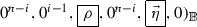
    Let ${\mathbb {B}}:=({{\varvec{b}}}_1,\ldots ,{{\varvec{b}}}_{3n+2})$ and ${\mathbb {B}}^*:=({{\varvec{b}}}^*_1,\ldots ,{{\varvec{b}}}^*_{3n+2})$ be dual orthonormal bases, ${\widehat{{\mathbb {B}}}}:= ({{\varvec{b}}}_1,..,{{\varvec{b}}}_{n+1},$${{\varvec{b}}}_{2n+2},$$..,{{\varvec{b}}}_{3n+2})$, , and , $\vec {\eta }_i,0)_{{{\mathbb {B}}}^*}$, where $i=1,..,n$, $\delta ,\rho ,\omega ,\tau \mathop {\leftarrow }\limits ^{{\textsf {U}}}{\mathbb {F}}_q$ and $\vec {\eta }_i\mathop {\leftarrow }\limits ^{{\textsf {U}}}{\mathbb {F}}_q^n$. Then, given ${\widehat{{\mathbb {B}}}}$, ${{\mathbb {B}}}^*$ and $\{{{\varvec{c}}}_i\}_{i=1,..,n}$, it is hard to tell $\{{{\varvec{k}}}_{0,i}\}_{i=1,..,n}$ from $\{{{\varvec{k}}}_{1,i}\}_{i=1,..,n}$. We then show the simplified version of Basic Problems 1 and 2 to Basic Problem 0 assumption, which implies the reduction of these assumptions to the DLIN assumption via the lowest level reduction (hierarchical reduction).

  • – The simplified version of Basic Problem 1 can be expressed as , and . Hence, it can be reduced to Basic Problem 0 for ciphertexts by embedding the Basic Problem 0 instance into the $(3n+2)$-dimensional space.

  • – The simplified version of Basic Problem 2 can be expressed as , , and . Hence, it can be reduced to Basic Problem 0 for secret keys by embedding the Basic Problem 0 instance into the $(3n+2)$-dimensional space, where the $\sigma$ part of the Basic Problem 0 element is embedded into the $\eta _i$ part with $(\eta _1,..,\eta _n) := \vec {\eta }$.

  The reductions from Basic Problems 1 and 2 to Basic Problem 0 are essentially the same as the above-mentioned middle-level reduction except that Basic Problems 1 and 2 have multiple spaces on bases (${{\mathbb {B}}}_t, {{\mathbb {B}}}^*_t$) with $t=0,1,..,d$, while the simplified version of Basic Problems 1 and 2 are on (${{\mathbb {B}}}, {{\mathbb {B}}}^*$) (Lemmas 15, 17 ).

  • Higher-Level Reductions Top-level assumptions, Problems 1 and 2 (Definitions 4, 5 ), are reduced to Basic Problems 1 and 2 by using Intra-subspace information theoretical transformation to be explained just below (see Lemmas 16, 18 for the reduction precisely). Problem 1 and 2 assumptions are used for computationally indistinguishable game changes of top level of security proof (full security proof of the proposed FE scheme). See Fig. 1 for the hierarchical structure of reductions.

• 2. Information theoretical transformations We have developed several information theoretical transformation techniques based on the property 2. of DPVS. There are two basic information theoretical techniques, intra-subspace and inter-subspace transformations, by the hidden base changes. Here we use the same example as that given in the property 2. of Sect. 1.3.2.

  Intra-subspace transformation:

  Hidden bases $({{\varvec{b}}}_{n+1},..,{{\varvec{b}}}_{N})$ and $({{\varvec{b}}}^*_{n+1},..,{{\varvec{b}}}^*_{N})$ are (conceptually) changed to $({{\varvec{d}}}_{n+1},..,{{\varvec{d}}}_{N}) := ({{\varvec{b}}}_{n+1},..,{{\varvec{b}}}_{N}) \cdot (Z^{-1})^{\mathrm {T}}$, and $({{\varvec{d}}}^*_{n+1},..,{{\varvec{d}}}^*_{N}):= ({{\varvec{b}}}^*_{n+1},..,{{\varvec{b}}}^*_{N})\cdot Z^{\mathrm {T}}$, where $Z \in GL(N-n,{\mathbb {F}}_q)$. We then have new dual orthonormal bases of ${\mathbb {V}}$, and 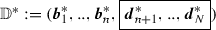. Then, ciphertext ${{\varvec{c}}}:= (\vec {\psi }_1, \vec {\psi }_2)_{{{\mathbb {B}}}}$ with $\vec {\psi }_i \in {\mathbb {F}}_q^n$ ($i=1,2$) can be expressed by , and secret key ${{\varvec{k}}}^* := (\vec {\xi }_1,\vec {\xi }_2)_{{{\mathbb {B}}}^*}$ with $\vec {\xi }_i \in {\mathbb {F}}_q^n$ ($i=1,2$) can be by .

  As mentioned above, the intra-subspace transformation is employed to reduce Problem 1 and 2 assumptions to Basic Problems 1 and 2.

  Inter-subspace transformation: Hidden bases $({{\varvec{b}}}_{n+1},..,{{\varvec{b}}}_{N})$ ($N=n+m$) and $({{\varvec{b}}}^*_{1},..,{{\varvec{b}}}^*_{n})$ are (conceptually) changed to $({{\varvec{d}}}_{n+1},..,$${{\varvec{d}}}_{N}) := ({{\varvec{b}}}_{n+1} - \sum _{j=1}^n f_{1,j} {{\varvec{b}}}_j, ..,{{\varvec{b}}}_{N} - \sum _{j=1}^n f_{m,j} {{\varvec{b}}}_j)$, and $({{\varvec{d}}}^*_{1},..,{{\varvec{d}}}^*_{n}):= ({{\varvec{b}}}^*_1 + \sum _{i=1}^m f_{i,1} {{\varvec{b}}}^*_{n+i}, .., {{\varvec{b}}}^*_n + \sum _{i=1}^m f_{i,n} {{\varvec{b}}}^*_{n+i}$, where $F := (f_{i,j}) \in {\mathbb {F}}_q^{\ m \times n}$. We then have new dual orthonormal bases of ${\mathbb {V}}$, and 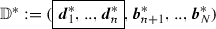. Then, ciphertext ${{\varvec{c}}}:= (\vec {\psi }_1, \vec {\psi }_2)_{{{\mathbb {B}}}}$ can be expressed by , and secret key ${{\varvec{k}}}^* := (\vec {\xi }_1,\vec {\xi }_2)_{{{\mathbb {B}}}^*}$ can be by .

The inter-subspace transformation is employed to prove the small advantage gaps between Game 2-$\nu$ and Game 3 in Fig. 1, where $F \mathop {\leftarrow }\limits ^{{\textsf {U}}}{\mathbb {F}}_q^{\ 1 \times 1}$ (a random scalar in ${\mathbb {F}}_q$) is employed. This transformation is also employed in the corresponding places in the security proof of Sects. F.2 and G , where more general forms of F are employed.

1.3.4 Non-monotone Policy

Non-monotone policies and predicates should be used in many FE applications. For example, an access policy (for a user) regarding a confidential audit report on ‘K Institute’ could be in the following form: NOT(Affiliation = ‘K Institute’) AND ($\cdots$).

To achieve a non-monotone policy on attributes in universe ${{{\mathcal {U}}}}$, it is essentially required to introduce a concept of categories or subuniverses, where a category or subuniverse, ${{{\mathcal {U}}}}_t$ ($t \in {\mathbb {N}}$ is an identity of a category), is a subset of universe ${{{\mathcal {U}}}}$. In the above-mentioned example, a subset of affiliations, ${{{\mathcal {U}}}}_{\textsf {affiliation}}$ is a category. Then, the policy on attribute X of a user is expressed as ($X \not =$ ‘K Institute’ $\wedge \ X \in {{{\mathcal {U}}}}_{\textsf {affiliation}}$) AND ($\cdots$).

Without such a notion of categories or subuniverses, a non-monotone policy cannot be correctly captured. For example, if a policy on attribute X is just ($X \not =$ ‘K Institute’) AND ($\cdots$), any attribute (e.g., ‘Professor’, ‘Male’, and ‘Japanese’) different from ‘K Institute’ in any category satisfies the clause with substituting such an attribute to X . (A straightforward application of a monotone ABE scheme [42] may have this problem.)

This paper presents an elegant solution to this issue by using dual subspaces of DPVS without using an explicit formula such as ($\ \ldots \ \wedge \ X \in {{{\mathcal {U}}}}_{\textsf {affiliation}}$). Here, an attribute is expressed by the form of $(t,x_t)$ with $t \in T \subseteq \{1,\ldots ,d\}$ in place of just an attribute x, where t identifies a subuniverse or category of attributes, and $x_t$ is an attribute in subuniverse t (examples of $(t,x_t)$ are (‘Affiliation’, ‘K Institute’), (‘Title’, ‘Professor’), (‘Gender’, ‘Male’) and (‘Nationality’, ‘Japanese’)).

In our scheme, each $(t,x_t)$ is encoded as a value in a subspace, ${\textsf {span}}\langle {\mathbb {B}}_t \rangle$, spanned by bases ${\mathbb {B}}_t$ (or ${\mathbb {B}}^*_t$) of DPVS, and a non-monotone policy on category t (e.g., $X_t \not =$ ‘K Institute’, $t =$ ‘Affiliation’) is also encoded in a subspace, ${\textsf {span}}\langle {\mathbb {B}}^*_t \rangle$, spanned by bases ${\mathbb {B}}^*_t$ (or ${\mathbb {B}}_t$), where independent d bases $({\mathbb {B}}_1,\ldots , {\mathbb {B}}_d)$ (and the dual bases, $({\mathbb {B}}^*_1, \ldots , {\mathbb {B}}^*_d)$) are set up in our scheme.

Roughly speaking, only a value in ${\textsf {span}}\langle {\mathbb {B}}_t \rangle$ can be correctly operated with a value in $\mathsf{span}\langle {\mathbb {B}}^*_t \rangle$. That is, only an attribute $x_t$ encoded in ${\textsf {span}}\langle {\mathbb {B}}_t \rangle$ can be correctly operated with a non-monotone policy on t (e.g., $X_t \not =$ ‘K Institute’) encoded in ${\textsf {span}}\langle {\mathbb {B}}^*_t \rangle$.

This can be formally ensured in the security proof by the fact that the information theoretical transformation via hidden base changes is shared by ${\textsf {span}}\langle {\mathbb {B}}_t \rangle$ and $\mathsf{span}\langle {\mathbb {B}}^*_t \rangle$, but it is perfectly independent from the other subspace spanned by different bases ${\mathbb {B}}_{t'}$ and ${\mathbb {B}}^*_{t'}$ with $t' \not = t$. In other words, the condition that $X \in {{{\mathcal {U}}}}_{\textsf {affiliation}}$ is realized in the correct operation mechanism between corresponding dual subspaces, ${\textsf {span}}\langle {\mathbb {B}}_t \rangle$ and ${\textsf {span}}\langle {\mathbb {B}}^*_t \rangle$. Hence, a non-monotone policy on t, $X_t \not =$ ‘K Institute’ with $t =$ ‘Affiliation’, can be correctly operated with an attribute of (‘Affiliation’, *) encoded in ${\textsf {span}}\langle {\mathbb {B}}^*_t \rangle$ but not with (‘Title,’ *) in ${\textsf {span}}\langle {\mathbb {B}}^*_{t'} \rangle$, ( ‘Gender’, *) in ${\textsf {span}}\langle {\mathbb {B}}^*_{t''} \rangle$, and (‘Nationality’, *) in ${\textsf {span}}\langle {\mathbb {B}}^*_{t'''} \rangle$.

More precisely, in our scheme, vectors, $\vec {x}$ and $\vec {v}$, are employed in place of attributes, and each vector is categorized to a category or subuniverse, ${{{\mathcal {U}}}}_t$, i.e., vector $\vec {x}$ in ${{{\mathcal {U}}}}_t$ is expressed by the form of $(t,\vec {x})$ and encoded in ${\textsf {span}}\langle {\mathbb {B}}_t \rangle$.

For example, in our KP-FE scheme, a ciphertext ${{\varvec{c}}}$ with a n-dimensional vector $(t,\vec {x})$ is realized as the form of

$$\begin{aligned} {{\varvec{c}}}:= ( \omega \vec {x}, 0^{n}, 0^{n}, \varphi )_{{{\mathbb {B}}}_t}, \end{aligned}$$

and a secret key ${{\varvec{k}}}^*_i$ for the ith entry of a negation term of a span program ($s_i$ is the corresponding share) associated with a vector $(t', \vec {v}_i)$ is of the form of

$$\begin{aligned} {{\varvec{k}}}^*_i := ( s_i \vec {v}_i, 0^{n_t}, \vec {\eta }_i, 0 )_{{{\mathbb {B}}}^*_{t'}}. \end{aligned}$$

Hence, in the decryption process,

$$\begin{aligned} e({{\varvec{c}}},{{\varvec{k}}}^*_i)^{1/\vec {x}\cdot \vec {v}_i} = g_T^{\omega s_i} \ \ \ \ \ (\hbox {iff}\, \,t=t' \hbox {and}\, \,\vec {x}\cdot \vec {v}_i\not =0). \end{aligned}$$

That is, due to the decryption property and the above-mentioned property that only $\vec {x}$ encoded in ${\textsf {span}}\langle {\mathbb {B}}_t \rangle$ can be correctly operated with $\vec {v}_i$ encoded in $\mathsf{span}\langle {\mathbb {B}}^*_t \rangle$, the ith share $s_i$ of the span program is recovered iff $t = t'$ and $\vec {x}\cdot \vec {v}_i\not =0$.

1.3.5 Adaptive Security

To achieve the adaptive security, this paper elaborately combines the dual system encryption technique proposed by Waters [49] and the DPVS methodology.

In the dual system encryption, roughly there are two forms of ciphertexts and secret keys, normal and semi-functional forms. One of the advantages of the DPVS methodology is that the two forms can be indistinguishable based on the above-mentioned Problems 1 and 2 assumptions, which are reduced to the DLIN assumption via the hierarchical reduction technique. See the security proof (outline) of Theorem 1 for more details of these forms and security game transformations.

In the security proof, we also apply the information theoretical technique using hidden bases in DPVS, which has been described above as the inter-subspace transformation.

1.4 Related Works

The definitional works for functional encryption were initiated by Boneh et al. [14] and O’Neill [41]. They presented two types of definitions, the simulation (SIM)-based one and the indistinguishability (IND)-based one. Boneh et al.  [14], Agrawal et al. [1] and Caro et al. [18] showed that a FE scheme with unbounded number of keys and ciphertexts in the standard model cannot be achieved in the SIM-based definition. Therefore, a fully secure functional encryption (with unbounded number of keys and ciphertexts) in the standard model should be realized in the IND-based definition.

As described before, there are two properties of functional encryption, attribute-hiding (or private-index) and payload-hiding (or public-index) [14, 30].

Although several FE schemes for general circuits or Turing machines are presented by using indistinguishable obfuscations (iO) or multi-linear maps [2, 22, 23, 26], while these primitives are currently on fragile ground and extremely inefficient.

The largest class of relations supported by a (public-index) FE scheme without using iO and multi-linear maps is general circuits [27]; however, they are not fully secure but selectively secure and still impractical.

To the best of our knowledge, the largest class of relations supported by a fully secure practical (public-index) FE scheme in the IND-based definition (with unbounded number of keys and ciphertexts) under a standard assumption in the standard model is non-monotone span programs with inner-product relations, which is achieved by this paper. The ABE scheme in [32] supports only monotone span programs with the equality relation, and the assumptions are non-standard on composite-order pairing groups. Spatial encryption [12, 19] supports a fairly large class of relations but still a limited class of those by the proposed scheme. Although some extensions of spatial encryption have been proposed [20], the relations supported by the scheme are also covered by those of the proposed FE scheme.

To the best of our knowledge, the largest class of a fully secure and (weakly) attribute-hiding practical FE scheme in the IND-based definition under reasonable assumptions in the standard model is the conjunction of inner-product relations (e.g., hierarchical inner-product relations and basic spacial encryption), which is achieved in this paper. The (H)IPE scheme in [32] is (weakly) attribute-hiding under a non-standard assumption.

Although an attribute-hiding FE scheme, (H)IPE scheme, specialized from the proposed FE scheme in this paper, is weakly attribute-hiding, fully-attribute-hiding (H)IPE schemes (in the IND-based definition) were presented under the same assumption, DLIN assumption, by [38, 39].

Our general access structures, i.e., span programs over inner-product predicates, have nice applications with sparse matrix DPVS techniques [40], for example, semi-adaptively secure KP-ABE scheme for span programs with constant-size ciphertexts (from DLIN) [46] and adaptively secure KP- and CP-ABE schemes from DLIN which allow attribute reuse in an available formula without the redundant multiple encoding technique given in “Appendix E” [47].

1.5 Notations

When A is a random variable or distribution, $y \mathop {\leftarrow }\limits ^{{\textsf {R}}}A$ denotes that y is randomly selected from A according to its distribution. When A is a set, $y \mathop {\leftarrow }\limits ^{{\textsf {U}}}A$ denotes that y is uniformly selected from A. $y := z$ denotes that y is set, defined or substituted by z. When a is a fixed value, $A(x) \rightarrow a$ (e.g., $A(x) \rightarrow 1$) denotes the event that machine (algorithm) A outputs a on input x. A function $f: {\mathbb {N}} \rightarrow {\mathbb {R}}$ is negligible in $\lambda$, if for every constant $c > 0$, there exists an integer n such that $f(\lambda ) < \lambda ^{-c}$ for all $\lambda > n$.

We denote the finite field of order q by ${\mathbb {F}}_q$, and ${\mathbb {F}}_q{\setminus } \{ 0 \}$ by ${{\mathbb {F}}_q^{\,\times }}$. A vector symbol denotes a vector representation over ${\mathbb {F}}_q$, e.g., $\vec {x}$ denotes $(x_{1},\ldots ,x_{n}) \in {\mathbb {F}}_q^{\, n}$. For two vectors $\vec {x} = (x_{1},\ldots ,x_{n})$ and $\vec {v} = (v_{1},\ldots ,v_{n})$, $\vec {x} \cdot \vec {v}$ denotes the inner-product $\sum _{i=1}^{n} x_i v_i$. The vector $\vec {0}$ is abused as the zero vector in ${\mathbb {F}}_q^{\, n}$ for any n. $X^{\mathrm T}$ denotes the transpose of matrix X. $I_\ell$ and $0_\ell$ denote the $\ell \times \ell$ identity matrix and the $\ell \times \ell$ zero matrix, respectively. A bold face letter denotes an element of vector space ${\mathbb {V}}$, e.g., ${{\varvec{x}}}\in {\mathbb {V}}$. When ${{\varvec{b}}}_i \in {\mathbb {V}}$ ($i=1,\ldots ,n$), ${\textsf {span}}\langle {{\varvec{b}}}_1, \ldots , {{\varvec{b}}}_n \rangle \subseteq {\mathbb {V}}$ (resp. ${\textsf {span}}\langle \vec {x}_1, \ldots , \vec {x}_n \rangle$) denotes the subspace generated by ${{\varvec{b}}}_1, \ldots , {{\varvec{b}}}_n$ (resp. $\vec {x}_1, \ldots , \vec {x}_n$). For vectors $\vec {x} := (x_1,\ldots ,x_N), \vec {y} := (y_1,\ldots ,y_N) \in {\mathbb {F}}_q^{\,N}$ and bases ${\mathbb {B}} := ({{\varvec{b}}}_1,\ldots ,{{\varvec{b}}}_N), {\mathbb {B}}^* := ({{\varvec{b}}}^*_1,\ldots ,{{\varvec{b}}}^*_N)$, $(\vec {x})_{\mathbb {B}} \ \left( = (x_1,\ldots ,x_N)_{\mathbb {B}} \right)$ denotes linear combination $\sum _{i=1}^{N} x_{i} {{\varvec{b}}}_i$, and $(\vec {y})_{{\mathbb {B}}^*} \ \left( = (y_1,\ldots ,y_N)_{{\mathbb {B}}^*} \right)$ denotes $\sum _{i=1}^{N} y_{i} {{\varvec{b}}}^*_i$. For a format of attribute vectors $\vec {n} := (d; n_1,\ldots ,n_d)$ that indicates dimensions of vector spaces, $\vec {e}_{t,j}$ denotes the canonical basis vector $(\overbrace{0\cdots 0}^{j-1},1,\overbrace{0\cdots 0}^{n_t-j}) \in {\mathbb {F}}_q^{\,n_t}$ for $t=1,\ldots ,d$ and $j=1,\ldots ,n_t$. $GL(n,{\mathbb {F}}_q)$ denotes the general linear group of degree n over ${\mathbb {F}}_q$.

2 Dual Pairing Vector Spaces (DPVS) and Main Lemmas

In this section, we present the notion of dual pairing vector spaces (DPVS) and a typical construction of DPVS from pairing groups. We also show main lemmas on DPVS, which are directly employed for the security proof of the proposed FE schemes.

2.1 DPVS by Direct Product of Symmetric Pairing Groups

In this paper, for simplicity of description, we will present the proposed schemes on the symmetric version of dual pairing vector spaces (DPVS) [35, 36] constructed using symmetric bilinear pairing groups given in Definition 1. Owing to the abstraction of DPVS, the presentation and the security proof of the proposed schemes are essentially the same as those on the asymmetric version of DPVS, $(q, {\mathbb {V}}, {\mathbb {V}}^*, {\mathbb {G}}_T, {{\mathbb {A}}}, {{\mathbb {A}}}^*, e)$, for which see “Appendix A.2”. The symmetric version is a specific (self-dual) case of the asymmetric version, where ${\mathbb {V}}= {\mathbb {V}}^*$ and ${{\mathbb {A}}}= {{\mathbb {A}}}^*$.

Definition 1

“Symmetric bilinear pairing groups” $(q,{\mathbb {G}},{\mathbb {G}}_T,G,e)$ are a tuple of a prime q, cyclic additive group ${\mathbb {G}}$ and multiplicative group ${\mathbb {G}}_T$ of order q, $G \ne 0 \in {\mathbb {G}}$, and a polynomial-time computable non-degenerate bilinear pairing $e: {\mathbb {G}}\times {\mathbb {G}}\rightarrow {\mathbb {G}}_T$, i.e., $e(sG ,tG) = e(G,G)^{st}$ and $e(G,G) \ne 1$.

Let ${{\mathcal {G}}}_{\textsf {bpg}}$ be an algorithm that takes input $1^{\lambda }$ and outputs a description of bilinear pairing groups $(q,{\mathbb {G}},{\mathbb {G}}_T,G,e)$ with security parameter $\lambda$.

Definition 2

“Dual pairing vector spaces (DPVS)” $(q, {\mathbb {V}}, {\mathbb {G}}_T, {{\mathbb {A}}}, e)$ by a direct product of symmetric pairing groups $(q,{\mathbb {G}},{\mathbb {G}}_T,G,e)$ are a tuple of prime q, ${N}$-dimensional vector space ${\mathbb {V}}:= \overbrace{{\mathbb {G}}\times \cdots \times {\mathbb {G}}}^{{N}}$ over ${\mathbb {F}}_q$, cyclic group ${\mathbb {G}}_T$ of order q, canonical basis ${{\mathbb {A}}}:= ({{\varvec{a}}}_1,\ldots ,{{\varvec{a}}}_{N})$ of ${\mathbb {V}}$, where ${{\varvec{a}}}_i := (\overbrace{0,\ldots ,0}^{i-1},G,$$\overbrace{0,\ldots ,0}^{{N}-i})$, and pairing $e : {\mathbb {V}}\times {\mathbb {V}}\rightarrow {\mathbb {G}}_T$.

The pairing is defined by $e({{\varvec{x}}},{{\varvec{y}}}) := \prod _{i=1}^N e(G_i,H_i) \in {\mathbb {G}}_T$ where ${{\varvec{x}}}:= (G_1,\ldots ,$$G_N) \in {\mathbb {V}}$ and ${{\varvec{y}}}:= (H_1,\ldots ,H_N) \in {\mathbb {V}}$. This is non-degenerate bilinear, i.e., $e(s {{\varvec{x}}},t {{\varvec{y}}}) = e({{\varvec{x}}},{{\varvec{y}}})^{st}$ and if $e({{\varvec{x}}},{{\varvec{y}}})=1$ for all ${{\varvec{y}}}\in {\mathbb {V}}$, then ${{\varvec{x}}}= {{\varvec{0}}}$. For all i and j, $e({{\varvec{a}}}_i, {{\varvec{a}}}_j) = e(G,G)^{\delta _{i,j}}$ where $\delta _{i,j} = 1$ if $i=j$, and 0 otherwise, and $e(G,G) \ne 1 \in {\mathbb {G}}_T$.

DPVS generation algorithm ${{{{{\mathcal {G}}}}_{\textsf {dpvs}}}}$ takes input $1^{\lambda }$ ($\lambda \in {\mathbb {N}}$) and ${N}\in {\mathbb {N}}$, and outputs a description of ${\textsf {param}}_{{\mathbb {V}}} := (q,{\mathbb {V}},{\mathbb {G}}_T,{{\mathbb {A}}}, e)$ with security parameter $\lambda$ and ${N}$-dimensional ${\mathbb {V}}$. It can be constructed using ${{\mathcal {G}}}_{\textsf {bpg}}$.

Remark 1

For matrix $W := ( w_{i,j})_{i,j =1,\ldots ,N} \in {\mathbb {F}}_q^{\,N \times N}$ and element ${{\varvec{g}}} := (G_1,\ldots ,G_N)$ in N-dimensional ${\mathbb {V}}$, ${{\varvec{g}}} W$ denotes $\textstyle {(\sum _{i=1}^{N} G_i w_{i,1}, \ldots , \sum _{i=1}^{N} G_i w_{i,N}) = }$$\textstyle (\sum _{i=1}^{N} w_{i,1} G_i, \ldots , \sum _{i=1}^{N} w_{i,N} G_i)$ by a natural multiplication of a N-dim. row vector and a $N \times N$ matrix. Thus, it holds an associative law as $({{\varvec{g}}} W) W^{-1} = {{\varvec{g}}} (W W^{-1}) = {{\varvec{g}}}$ and a pairing invariance property $e({{\varvec{g}}} W, {{\varvec{h}}}(W^{-1})^{\mathrm{{T}}}) = e({{\varvec{g}}}, {{\varvec{h}}})$ for any ${{\varvec{g}}},{{\varvec{h}}}\in {\mathbb {V}}$.

We describe random dual orthonormal basis generator ${{{{{\mathcal {G}}}}_{\textsf {ob}}}}$ below, which is used as a subroutine in the proposed FE scheme.

$$\begin{aligned}&{{{{{\mathcal {G}}}}_{\textsf {ob}}}}(1^{\lambda },\vec {n} := (d; n_1, \ldots , n_d)) : \mathsf{param}_{\mathbb {G}}:= (q,{\mathbb {G}},{\mathbb {G}}_T,{G},e) \mathop {\leftarrow }\limits ^{{\textsf {R}}}{{{\mathcal {G}}}}_\mathsf{bpg}(1^{\lambda }), \ \ \psi \mathop {\leftarrow }\limits ^{{\textsf {U}}}{{\mathbb {F}}_q^{\,\times }},\\&\quad {N}_0 := 5, \ \ {N}_t := 3 n_t + 1 \ \ \mathrm {for} \ t=1,\ldots ,d,\\&\quad \hbox {for} \ t = 0,\ldots ,d, \\&\ \ \quad {\textsf {param}}_{{\mathbb {V}}_t} := (q, {\mathbb {V}}_t, {\mathbb {G}}_T, {{\mathbb {A}}}_t, e) := {{{{{\mathcal {G}}}}_{\textsf {dpvs}}}}(1^{\lambda }, {N}_t, \mathsf{param}_{\mathbb {G}}), \\&\quad \begin{aligned} X_t&:= \left( \begin{array}{c} \vec {\chi }_{t,1} \\ \vdots \\ \vec {\chi }_{t,N_t} \end{array} \right) := (\chi _{t,i,j})_{i,j} \mathop {\leftarrow }\limits ^{{\textsf {U}}}GL({N}_t, {\mathbb {F}}_q), \left( \begin{array}{c} \vec {\vartheta }_{t,1} \\ \vdots \\ \vec {\vartheta }_{t,N_t} \end{array} \right) := (\vartheta _{t,i,j})_{i,j} := \psi \cdot (X_t^{\text {T}})^{-1}, \end{aligned}\\&\ \ \ \ \ \quad {\textstyle {{\varvec{b}}}_{t,i} := (\vec {\chi }_{t,i})_{{{\mathbb {A}}}_t} = \sum _{j=1}^{{N}_t} \chi _{t,i,j} {{\varvec{a}}}_{t,j} \ \ \mathrm {for} \ i=1,\ldots ,N_t, \ \ {{\mathbb {B}}}_t := ({{\varvec{b}}}_{t,1},\ldots ,{{\varvec{b}}}_{t,{N}_t}), } \\&\ \ \ \ \ \ \ \ { {{\varvec{b}}}^{*}_{t,i} := (\vec {\vartheta }_{t,i})_{{{\mathbb {A}}}_t} = \sum _{j=1}^{{N}_t} \vartheta _{t,i,j} {{\varvec{a}}}_{t,j} \ \ \mathrm {for} \ i=1,\ldots ,N_t, \ \ {{\mathbb {B}}}_t^{*} := ({{\varvec{b}}}^{*}_{t,1},\ldots ,{{\varvec{b}}}^{*}_{t,{N}_t}), } \\&\ \ \ g_T := e({G}, {G})^\psi , \ \ {\textsf {param}}_{\vec {n}} := (\{ {\textsf {param}}_{{\mathbb {V}}_t} \}_{t=0,\ldots ,d}, \ g_T), \\&\ \ \ \mathrm{return} \ \ ({\textsf {param}}_{\vec {n}}, \{ {{\mathbb {B}}}_t, {{\mathbb {B}}}_t^* \}_{t=0,\ldots ,d}). \ \ \ \ \ \ \ \ \ \ \ \ \ \ \ \ \ \ \ \ \ \ \ \ \ \ \ \ \ \ \ \ \ \ \ \ \ \ \ \ \ \ \ \ \ \ \ \ \ \ \ \ \ \ \ \ \ \ \ \ \ \ \ \ \ \ \end{aligned}$$

We note that $g_T = e({{\varvec{b}}}_{t,i}, {{\varvec{b}}}^*_{t,i})$ for $t=0,\ldots ,d; i=1,\ldots ,{N}_t$.

2.2 Decisional Linear (DLIN) Assumption

Definition 3

(DLIN: decisional linear assumption [9]) The DLIN problem is to guess $\beta \in \{ 0,1 \}$, given $( \mathsf{param}_{{\mathbb {G}}}, \ {G},{\xi }{G},{\kappa }{G},\delta {\xi }{G}, \sigma {\kappa }{G}, Y_\beta ) \mathop {\leftarrow }\limits ^{{\textsf {R}}}{{{{\mathcal {G}}}}}_{\beta }^\mathsf{DLIN}(1^{\lambda })$, where

$$\begin{aligned}&{{{{\mathcal {G}}}}}_{\beta }^{\textsf {DLIN}}(1^{\lambda }): {\textsf {param}}_{{\mathbb {G}}} := (q,{\mathbb {G}},{\mathbb {G}}_T,{G},e) \mathop {\leftarrow }\limits ^{{\textsf {R}}}{{{\mathcal {G}}}}_{\textsf {bpg}}(1^{\lambda }),\\&\quad {\kappa }, \delta , {\xi },\sigma \mathop {\leftarrow }\limits ^{{\textsf {U}}}{\mathbb {F}}_q, \ \ \ Y_0 := (\delta + \sigma ) {G}, \ \ \ Y_1 \mathop {\leftarrow }\limits ^{{\textsf {U}}}{\mathbb {G}},\\&\quad \mathrm{return} \ \ ( {\textsf {param}}_{{\mathbb {G}}}, \ {G},{\xi }{G}, {\kappa }{G}, \delta {\xi }{G}, \sigma {\kappa }{G}, Y_\beta ), \end{aligned}$$

for $\beta \mathop {\leftarrow }\limits ^{{\textsf {U}}}\{0,1\}$. For a probabilistic machine ${{{\mathcal {E}}}}$, we define the advantage of ${{{\mathcal {E}}}}$ for the DLIN problem as:

$$\begin{aligned}&\mathsf{Adv}^{\textsf {DLIN}}_{{{{\mathcal {E}}}}}(\lambda ) := \textstyle \left| {\textsf {Pr}}\left[ {{{\mathcal {E}}}}(1^{\lambda },\varrho ) \! \rightarrow \! 1 \left| \ \varrho \mathop {\leftarrow }\limits ^{{\textsf {R}}}\! {{{{{\mathcal {G}}}}}_0^{\textsf {DLIN}}}(1^{\lambda }) \right. \right] \!\right. \left. - {\textsf {Pr}}\left[ {{{\mathcal {E}}}}(1^{\lambda },\varrho ) \! \rightarrow \! 1 \left| \ \varrho \mathop {\leftarrow }\limits ^{{\textsf {R}}}\! {{{{{\mathcal {G}}}}}_1^{\textsf {DLIN}}}(1^{\lambda }) \right. \right] \right| . \end{aligned}$$

The DLIN assumption is: For any probabilistic polynomial-time adversary ${{{\mathcal {E}}}}$, the advantage $\mathsf{Adv}^{\textsf {DLIN}}_{{{{\mathcal {E}}}}}(\lambda )$ is negligible in $\lambda$.

2.3 Main Lemmas (Lemmas 1, 2 and 3 )

We will show three lemmas directly employed in the proof of Theorems 1 and 2 . The proofs of the lemmas are given in “Appendix B”.

Definition 4

(Problem 1) Problem 1 is to guess $\beta$, given $({\textsf {param}}_{\vec {n}}, {{\mathbb {B}}}_0, {\widehat{{\mathbb {B}}}}^*_0,{{\varvec{e}}}_{\beta ,0}, \{ {{\mathbb {B}}}_t, {\widehat{{\mathbb {B}}}}^*_t, {{\varvec{e}}}_{\beta ,t,1},$${{\varvec{e}}}_{t,i} \}_{t=1,\ldots ,d; i=2,\ldots ,n_t} ) \mathop {\leftarrow }\limits ^{{\textsf {R}}}{{{{\mathcal {G}}}}}_{\beta }^\mathsf{P1}(1^{\lambda }, \vec {n})$, where

$$\begin{aligned}&{{{{\mathcal {G}}}}}_{\beta }^{\textsf {P1}}(1^{\lambda }, \vec {n}): \ \ \ (\mathsf{param}_{\vec {n}}, \{ {{\mathbb {B}}}_t, {{\mathbb {B}}}^{*}_t \}_{t=0,\ldots ,d}) \mathop {\leftarrow }\limits ^{{\textsf {R}}}{{{{{\mathcal {G}}}}_{\textsf {ob}}}}(1^{\lambda },\vec {n}), \\&\ \ \ {\widehat{{\mathbb {B}}}}^*_0 := ({{\varvec{b}}}^*_{0,1},{{\varvec{b}}}^*_{0,3},..,{{\varvec{b}}}^*_{0,5}), \ {\widehat{{\mathbb {B}}}}^*_t := ({{\varvec{b}}}^*_{t,1},.., {{\varvec{b}}}^*_{t,n_t}, {{\varvec{b}}}^*_{t,2n_t+1},.., {{\varvec{b}}}^*_{t,3n_t+1}) \ \ \mathrm {for} \ t=1,..,d, \\&\ \ \ \omega , z_0, \gamma _0 \mathop {\leftarrow }\limits ^{{\textsf {U}}}{\mathbb {F}}_q, \ \ \ {{\varvec{e}}}_{0,0} := (\omega , 0, 0, 0, \gamma _0)_{{{\mathbb {B}}}_0}, \ \ \ {{\varvec{e}}}_{1,0} := (\omega , z_0, 0, 0, \gamma _0)_{{{\mathbb {B}}}_0}, \\&\ \ \ \mathrm {for } \ t=1,\ldots ,d; \\&\ \ \ \ \ \ \ \ \vec {e}_{t,1} := (1,0^{n_t-1}) \in {\mathbb {F}}_q^{\,n_t}, \ \vec {z}_{t} \mathop {\leftarrow }\limits ^{{\textsf {U}}}{\mathbb {F}}_q^{\,n_t}, \ \gamma _t \mathop {\leftarrow }\limits ^{{\textsf {U}}}{\mathbb {F}}_q, \\&\ \ \ \ \ \ \ \ \begin{array}{lccccccc} &{} &{} \overbrace{\ \ \ \ \ \ \ \ \ \ \ \ \ }^{n_t} &{} \quad \overbrace{\ \ \ \ \ \ \ \ \ \ \ \ \ }^{n_t} &{}\quad \overbrace{\ \ \ \ \ \ \ \ \ \ \ \ \ }^{n_t} &{}\quad \overbrace{\ }^{1} \\ {{\varvec{e}}}_{0,t,1} := &{}(&{}\quad \omega \vec {e}_{t,1}, &{}\quad 0^{n_t}, &{} \quad 0^{n_t},&{}\quad \gamma _{t} &{} )_{{{\mathbb {B}}}_t}, \\ {{\varvec{e}}}_{1,t,1} := &{}(&{}\quad \omega \vec {e}_{t,1}, &{}\quad \vec {z}_{t}, &{}\quad 0^{n_t}, &{} \quad \gamma _{t} &{} )_{{{\mathbb {B}}}_t}, \end{array} \\&\ \ \ \ \ \ \ \ {{\varvec{e}}}_{t,i} := \omega {{\varvec{b}}}_{t,i} \ \ \mathrm {for} \ i=2,\ldots ,n_t, \\&\ \ \ \mathrm{return} \ \ ({\textsf {param}}_{\vec {n}}, {{\mathbb {B}}}_0, {\widehat{{\mathbb {B}}}}^*_0,{{\varvec{e}}}_{\beta ,0}, \{ {{\mathbb {B}}}_t, {\widehat{{\mathbb {B}}}}^*_t, {{\varvec{e}}}_{\beta ,t,1}, {{\varvec{e}}}_{t,i} \}_{t=1,\ldots ,d; i=2,\ldots ,n_t} ), \end{aligned}$$

for $\beta \mathop {\leftarrow }\limits ^{{\textsf {U}}}\{0,1\}$. For a probabilistic machine ${{{\mathcal {B}}}}$, we define the advantage of ${{{\mathcal {B}}}}$ as the quantity

$$\begin{aligned} \mathsf{Adv}^{\textsf {P1}}_{{{{\mathcal {B}}}}}(\lambda ) \! := \! {\textstyle \left| {\textsf {Pr}}\! \left[ {{{\mathcal {B}}}}(1^{\lambda }, \varrho ) \! \rightarrow \! 1 \left| \varrho \mathop {\leftarrow }\limits ^{{\textsf {R}}}\! {{{{\mathcal {G}}}}}_0^{\textsf {P1}}(1^{\lambda }, \! \vec {n}) \! \right. \right] \! - \! {\textsf {Pr}}\! \left[ {{{\mathcal {B}}}}(1^{\lambda }, \varrho ) \! \rightarrow \! 1 \left| \varrho \mathop {\leftarrow }\limits ^{{\textsf {R}}}\! {{{{\mathcal {G}}}}}_1^{\textsf {P1}}(1^{\lambda }, \! \vec {n}) \! \right. \right] \right| . } \end{aligned}$$

Lemma 1

For any adversary ${{{\mathcal {B}}}}$, there exist probabilistic machines ${{{\mathcal {E}}}}$, whose running times are essentially the same as that of ${{{\mathcal {B}}}}$, such that for any security parameter $\lambda$, $\mathsf{Adv}^\mathsf{P1}_{{{{\mathcal {B}}}}}(\lambda ) \le \mathsf{Adv}^{\textsf {DLIN}}_{{{{\mathcal {E}}}}}(\lambda ) + (d+6)/q.$

Definition 5

(Problem 2) Problem 2 is to guess $\beta$, given $({\textsf {param}}_{\vec {n}}, {\widehat{{\mathbb {B}}}}_0, {{\mathbb {B}}}^*_0, {{\varvec{h}}}^*_{\beta ,0}, {{\varvec{e}}}_0, \{{\widehat{{\mathbb {B}}}}_t, {{\mathbb {B}}}^*_t,$${{\varvec{h}}}^{*}_{\beta ,t,i}, {{\varvec{e}}}_{t,i} \}_{t=1,\ldots ,d; i=1,\ldots ,n_t} ) \mathop {\leftarrow }\limits ^{{\textsf {R}}}{{{{\mathcal {G}}}}}_{\beta }^\mathsf{P2}(1^{\lambda }, \vec {n})$, where

$$\begin{aligned}& {{{{\mathcal {G}}}}}_{\beta }^{\textsf {P2}}(1^{\lambda }, \vec {n}): \ \ \ (\mathsf{param}_{\vec {n}}, \{ {{\mathbb {B}}}_t, {{\mathbb {B}}}^{*}_t \}_{t=0,\ldots ,d}) \mathop {\leftarrow }\limits ^{{\textsf {R}}}{{{{{\mathcal {G}}}}_{\textsf {ob}}}}(1^{\lambda },\vec {n}), \\& \ \ \ {\widehat{{\mathbb {B}}}}_0 := ({{\varvec{b}}}_{0,1},{{\varvec{b}}}_{0,3},..,{{\varvec{b}}}_{0,5}), \ {\widehat{{\mathbb {B}}}}_t \!:=\! ({{\varvec{b}}}_{t,1},..,{{\varvec{b}}}_{t,n_t}, {{\varvec{b}}}_{t,2n_t+1},..,{{\varvec{b}}}_{t,3n_t+1}) \ \ \ \mathrm {for} \ t\!=\!1,..,d, \\& \ \ \ \delta , \delta _{0}, \omega \mathop {\leftarrow }\limits ^{{\textsf {U}}}{\mathbb {F}}_q, \ \tau , u_0 \mathop {\leftarrow }\limits ^{{\textsf {U}}}{{\mathbb {F}}_q^{\,\times }}, \ z_{0} := u_0^{-1}, \\& \ \ \ \left( \begin{array}{c} \vec {z}_{t,1} \\ \vdots \\ \vec {z}_{t,n_t} \end{array} \right) := Z_t \mathop {\leftarrow }\limits ^{{\textsf {U}}}GL(n_t,{\mathbb {F}}_q), \ \left( \begin{array}{c} \vec {u}_{t,1} \\ \vdots \\ \vec {u}_{t,n_t} \end{array} \right) := (Z_t^{-1})^{\mathrm{T}} \ \mathrm {for} \ t=1,..,d, \\&\ \ \ {{\varvec{h}}}^{*}_{0,0} := (\delta , 0, 0, \delta _{0}, 0)_{{{\mathbb {B}}}^*_0},\ {{\varvec{h}}}^{*}_{1,0} := (\delta , u_{0}, 0, \delta _{0}, 0)_{{{\mathbb {B}}}^*_0},\ {{\varvec{e}}}_{0} := (\omega , \tau z_0, 0, 0, 0)_{{{\mathbb {B}}}_0}, \\&\ \ \ \mathrm {for } \ t=1,\ldots ,d; \ i=1,\ldots , n_t; \\&\ \ \ \ \ \vec {e}_{t,i} := (0^{i-1},1,0^{n_t-i}) \in {\mathbb {F}}_q^{\,n_t}, \ \ \vec {\delta }_{t,i} \mathop {\leftarrow }\limits ^{{\textsf {U}}}{\mathbb {F}}_q^{\,n_t}, \\&\ \ \ \ \ \begin{array}{lccccccc} &{} &{} \overbrace{\ \ \ \ \ \ \ \ \ \ \ \ \ \ \ \ \ }^{n_t} &{}\quad \overbrace{\ \ \ \ \ \ \ \ \ \ \ \ \ \ \ \ \ }^{n_t} &{}\quad \overbrace{\ \ \ \ \ \ \ \ \ \ \ \ \ \ \ \ \ }^{n_t} &{}\quad \overbrace{\ }^{1} \\ {{\varvec{h}}}^{*}_{0,t,i} := &{}(&{}\quad \delta \vec {e}_{t,i}, &{} 0^{n_t}, &{}\quad \vec {\delta }_{t,i},&{} \quad 0 &{} )_{{{\mathbb {B}}}^*_t} &{} \\ {{\varvec{h}}}^{*}_{1,t,i} := &{}(&{}\quad \delta \vec {e}_{t,i}, &{}\quad \vec {u}_{t,i}, &{}\quad \vec {\delta }_{t,i}, &{}\quad 0 &{} )_{{{\mathbb {B}}}^*_t} &{} \\ {{\varvec{e}}}_{t,i} := &{}(&{} \quad \omega \vec {e}_{t,i}, &{}\quad \tau \vec {z}_{t,i},&{}\quad 0^{n_t},&{} \quad 0 &{} )_{{{\mathbb {B}}}_t}, \end{array} \\&\ \ \ \mathrm{return} \, ({\textsf {param}}_{\vec {n}}, {\widehat{{\mathbb {B}}}}_0, {{\mathbb {B}}}^*_0, {{\varvec{h}}}^*_{\beta ,0}, {{\varvec{e}}}_0, \{ {\widehat{{\mathbb {B}}}}_t, {{\mathbb {B}}}^*_t, {{\varvec{h}}}^{*}_{\beta ,t,i}, {{\varvec{e}}}_{t,i} \}_{t=1,..,d; i=1,..,n_t} ), \end{aligned}$$

for $\beta \mathop {\leftarrow }\limits ^{{\textsf {U}}}\{0,1\}$. For a probabilistic adversary ${{{\mathcal {B}}}}$, the advantage of ${{{\mathcal {B}}}}$ for Problem 2, $\mathsf{Adv}^{\textsf {P2}}_{{{{\mathcal {B}}}}}(\lambda )$, is similarly defined as in Definition 4.

Lemma 2

For any adversary ${{{\mathcal {B}}}}$, there exists a probabilistic machine ${{{\mathcal {E}}}}$, whose running time is essentially the same as that of ${{{\mathcal {B}}}}$, such that for any security parameter $\lambda$, $\mathsf{Adv}^{\textsf {P2}}_{{{{\mathcal {B}}}}}(\lambda ) \le \mathsf{Adv}^{\textsf {DLIN}}_{{{{\mathcal {E}}}}}(\lambda ) + 5/q.$

Lemma 3

For $p \in {\mathbb {F}}_q$, let $C_p := \{ (\vec {x},\vec {v}) | \vec {x} \cdot \vec {v} = p, \vec {x} \ne \vec {0}, \vec {v} \ne \vec {0} \} \subset {\mathbb {F}}_q^{\,n} \times {\mathbb {F}}_q^{\,n}$. For all $(\vec {x},\vec {v}) \in C_p$, for all $(\vec {r},\vec {w}) \in C_p$, $\Pr \left[ \vec {x} U = \vec {r} \ \wedge \ \vec {v} Z = \vec {w} \right]$$= \Pr \left[ \vec {x} Z = \vec {r} \ \wedge \ \vec {v} U = \vec {w} \right] = 1 \big / \sharp \,C_p,$ where $Z \mathop {\leftarrow }\limits ^{{\textsf {U}}}GL(n,{\mathbb {F}}_q), U := (Z^{-1})^{\mathrm {T}}$.

3 Functional Encryption with a Large Class of Relations

In this section, we provide the definition of functional encryption with a large class of relations, which are specified by non-monotone access structures combined with inner-product relations.

As described in Sect. 1.3.4, vectors, $\vec {x}$ and $\vec {v}$, with a ciphertext and secret key are expressed by the form of $(t,\vec {x})$ and $(t,\vec {v})$, which mean that $\vec {x}$ and $\vec {v}$ are in a category or subuniverse, ${{{\mathcal {U}}}}_t$, i.e., t is the identity of a category or subuniverse, ${{{\mathcal {U}}}}_t$.

Non-monotone access structures can be realized by span programs (Definition 6) and be combined with inner-product relations (Definition 7).

3.1 Span Programs and Non-Monotone Access Structures

Definition 6

(Span programs [4]) Let $\{p_1,\ldots ,p_n\}$ be a set of variables. A span program over ${\mathbb {F}}_q$ is a labeled matrix ${\hat{M}} := (M,\rho )$ where M is a (${\ell }\times {r}$) matrix over ${\mathbb {F}}_q$ and $\rho$ is a labeling of the rows of M by literals from $\{p_1,\ldots ,p_n,\lnot p_1,\ldots ,$$\lnot p_n\}$ (every row is labeled by one literal), i.e., $\rho : \{1,\ldots ,{\ell }\} \rightarrow \{p_1,\ldots ,p_n,\lnot p_1,$$\ldots ,$$\lnot p_n\}$.

A span program accepts or rejects an input by the following criterion. For every input sequence $\delta \in \{0,1\}^n$ define the submatrix $M_\delta$ of M consisting of those rows whose labels are set to 1 by the input $\delta$, i.e., either rows labeled by some $p_i$ such that $\delta _i = 1$ or rows labeled by some $\lnot p_i$ such that $\delta _i = 0$. (i.e., $\gamma : \{1,\ldots ,{\ell }\} \rightarrow \{0,1\}$ is defined by $\gamma (j)= 1$ if $[\rho (j)= p_i] \wedge [\delta _i = 1]$ or $[\rho (j)= \lnot p_i] \wedge [\delta _i = 0]$, and $\gamma (j)= 0$ otherwise. $M_\delta := (M_j)_{\gamma (j)=1}$, where $M_j$ is the jth row of M.)

The span program ${\hat{M}}$ accepts $\delta$ if and only if $\vec {1} \in {\textsf {span}}\langle M_\delta \rangle$, i.e., some linear combination of the rows of $M_\delta$ gives the all one vector $\vec {1}$. (The row vector has the value 1 in each coordinate.) A span program computes a Boolean function f if it accepts exactly those inputs $\delta$ where $f(\delta )=1$.

A span program is called monotone if the labels of the rows are only the positive literals $\{p_1,\ldots ,p_n\}$. Monotone span programs compute monotone functions. (So, a span program in general is “non”-monotone.)

We assume that no row $M_i$$(i=1,\ldots ,{\ell })$ of the matrix M is $\vec {0}$. We now introduce a non-monotone access structure with evaluating map $\gamma$ by using the inner-product of attribute vectors, that is employed in the proposed functional encryption schemes.

Definition 7

(Inner-products of attribute vectors and access structures) ${{{\mathcal {U}}}}_t$ ($t=1,$$\ldots , d$ and ${{{\mathcal {U}}}}_t \subset \{0,1\}^*$) is a subuniverse, a set of vectors, each of which is expressed by a pair of subuniverse id and $n_t$-dimensional vector, i.e., $(t,\vec {v})$, where $t \in \{1,\ldots ,d\}$ and $\vec {v} \in {\mathbb {F}}_q^{\,n_t} {\setminus } \{ \vec {0} \}$.

We now define such an attribute to be a variable p of a span program ${\hat{M}}:=(M,\rho )$, i.e., $p := (t,\vec {v})$. An access structure ${{\mathbb {S}}}$ is span program ${\hat{M}} := (M,\rho )$ along with variables $p:= (t,\vec {v}), p':= (t',\vec {v}'),\ldots$, i.e., ${{\mathbb {S}}}:= (M, \rho )$ such that $\rho : \{1,\ldots ,{\ell }\} \rightarrow \{ (t,\vec {v}), (t',\vec {v}'),\ldots$, $\lnot (t,\vec {v}), \lnot (t',\vec {v}'),\ldots \}$.

Let $\Gamma$ be a set of attributes, i.e., $\Gamma := \{ (t, \vec {x}_t) \mid \vec {x}_t \in {\mathbb {F}}_q^{\,n_t} {\setminus } \{ \vec {0} \}, 1 \le t \le d \}$, where $1 \le t \le d$ means that t is an element of some subset of $\{1,\ldots ,d\}$.

When $\Gamma$ is given to access structure ${{\mathbb {S}}}$, map $\gamma : \{1,\ldots ,{\ell }\} \rightarrow \{0,1\}$ for span program ${\hat{M}}:=(M,\rho )$ is defined as follows: For $i = 1,\ldots , {\ell }$, set $\gamma (i) = 1$ if $[\rho (i)=(t,\vec {v}_i)]$$\wedge [(t,\vec {x}_{t}) \in \Gamma ]$$\wedge [\vec {v}_i\cdot \vec {x}_{t} = 0]$ or $[\rho (i)=\lnot (t,\vec {v}_i)]$$\wedge [(t,\vec {x}_{t}) \in \Gamma ]$$\wedge [\vec {v}_i\cdot \vec {x}_{t} \not = 0]$. Set $\gamma (i) = 0$ otherwise.

Access structure ${{\mathbb {S}}}:= (M,\rho )$ accepts $\Gamma$ iff $\vec {1} \in {\textsf {span}}\langle (M_i)_{\gamma (i)=1} \rangle$.

Remark 2

The restriction that $\vec {v} \ne \vec {0}$ and $\vec {x}_t \ne \vec {0}$ above is required by the security proof or more specifically by Lemma 3. This restriction is reasonable in many applications. For example, in the equality relations for ABE, $\vec {v} := (v,-1)$ and $\vec {x} := (1, x)$, where $v=x$ iff $\vec {v}\cdot \vec {x} = 0$.

We now construct a secret-sharing scheme for a non-monotone access structure or span program.

Definition 8

A secret-sharing scheme for span program ${\hat{M}}:=(M,\rho )$ is:

• 1. Let M be ${\ell }\times {r}$ matrix. Let column vector $\vec {f}^{\mathrm{T}}:=(f_1,\ldots ,f_{r})^{\mathrm{T}}$$\mathop {\leftarrow }\limits ^{{\textsf {U}}}{\mathbb {F}}_q^{\,{r}}$. Then, $s_0 := \vec {1}\cdot \vec {f}^{\mathrm{T}} = \sum _{k=1}^{r}f_k$ is the secret to be shared, and $\vec {s}^{\mathrm{T}} := (s_1,\ldots ,s_{\ell })^{\mathrm{T}} := M\cdot \vec {f}^{\mathrm{T}}$ is the vector of ${\ell }$ shares of the secret $s_0$ and the share $s_i$ belongs to $\rho (i)$.

• 2. If span program ${\hat{M}}:=(M,\rho )$ accept $\delta$, or access structure ${{\mathbb {S}}}:= (M,\rho )$ accepts $\Gamma$, i.e., $\vec {1} \in {\textsf {span}}\langle (M_i)_{\gamma (i)=1} \rangle$ with $\gamma : \{1,\ldots ,{\ell }\} \rightarrow \{0,1\}$, then there exist constants $\{ \alpha _i \in {\mathbb {F}}_q\mid i \in I \}$ such that $I \subseteq \{ i \in \{ 1, \ldots , {\ell }\} \mid \gamma (i)=1 \}$ and $\sum _{i \in I} \alpha _i s_i = s_0$. Furthermore, these constants $\{ \alpha _i \}$ can be computed in time polynomial in the size of matrix M.

3.2 Key-Policy Functional Encryption with a Large Class of Relations

Definition 9

(Key-policy functional encryption: KP-FE) A key-policy functional encryption scheme consists of four algorithms.

${\textsf {Setup}}$ :

This is a randomized algorithm that takes as input security parameter and format $\vec {n} := (d; n_1,\ldots ,n_d)$ of attributes. It outputs public parameters pk and master secret key sk.

${\textsf {KeyGen}}$ :

This is a randomized algorithm that takes as input access structure ${{\mathbb {S}}}:= (M, \rho )$, pk and sk. It outputs a decryption key ${\textsf {sk}}_{{\mathbb {S}}}$.

${\textsf {Enc}}$ :

This is a randomized algorithm that takes as input message m, a set of attributes, $\Gamma := \{ (t,\vec {x}_t) | \vec {x}_t$$\in {\mathbb {F}}_q^{\,n_t} {\setminus } \{ \vec {0} \}, 1 \le t \le d \}$, and public parameters pk. It outputs a ciphertext ${\textsf {ct}}_{\Gamma }$.

${\textsf {Dec}}$ :

This takes as input ciphertext ${\textsf {ct}}_{\Gamma }$ that was encrypted under a set of attributes $\Gamma$, decryption key $\mathsf{sk}_{{\mathbb {S}}}$ for access structure ${{\mathbb {S}}}$, and public parameters pk. It outputs either plaintext m or the distinguished symbol $\bot$.

A KP-FE scheme should have the following correctness property: for all $({\textsf {pk}}, {\textsf {sk}}) \mathop {\leftarrow }\limits ^{{\textsf {R}}}{\textsf {Setup}}(1^{\lambda },$$\vec {n})$, all access structures ${{\mathbb {S}}}$, all decryption keys $\mathsf{sk}_{{{\mathbb {S}}}} \mathop {\leftarrow }\limits ^{{\textsf {R}}}{\textsf {KeyGen}}({\textsf {pk}}, {\textsf {sk}}, {{\mathbb {S}}})$, all messages m, all attribute sets $\Gamma$, all ciphertexts ${\textsf {ct}}_{\Gamma } \mathop {\leftarrow }\limits ^{{\textsf {R}}}{\textsf {Enc}}({\textsf {pk}},$$m, \Gamma )$, it holds that $m = {\textsf {Dec}}({\textsf {pk}}, \mathsf{sk}_{{{\mathbb {S}}}}, {\textsf {ct}}_{\Gamma })$ with overwhelming probability, if ${{\mathbb {S}}}$ accepts $\Gamma$.

Definition 10

The model for proving the adaptively payload-hiding security of KP-FE under chosen-plaintext attack is:

Setup :

The challenger runs the setup algorithm, $({\textsf {pk}}, \mathsf{sk})\mathop {\leftarrow }\limits ^{{\textsf {R}}}{\textsf {Setup}}(1^{\lambda }, \ \vec {n})$, and gives public parameters ${\textsf {pk}}$ to the adversary.

Phase 1 :

The adversary is allowed to adaptively issue a polynomial number of queries, ${{\mathbb {S}}}$, to the challenger or oracle $\mathsf{KeyGen}({\textsf {pk}}, {\textsf {sk}}, \cdot )$ for private keys, $\mathsf{sk}_{{\mathbb {S}}}$ associated with ${{\mathbb {S}}}$.

Challenge :

The adversary submits two messages $m^{(0)}, m^{(1)}$ and a set of attributes, $\Gamma$, provided that no ${{\mathbb {S}}}$ queried to the challenger in Phase 1 accepts $\Gamma$. The challenger flips a coin $b \mathop {\leftarrow }\limits ^{{\textsf {U}}}\{ 0,1 \}$, and computes ${\textsf {ct}}_{\Gamma }^{(b)}\mathop {\leftarrow }\limits ^{{\textsf {R}}}\mathsf{Enc}({\textsf {pk}},m^{(b)},\Gamma )$. It gives ${\textsf {ct}}_{\Gamma }^{(b)}$ to the adversary.

Phase 2 :

The adversary is allowed to adaptively issue a polynomial number of queries, ${{\mathbb {S}}}$, to the challenger or oracle $\mathsf{KeyGen}({\textsf {pk}}, {\textsf {sk}}, \cdot )$ for private keys, $\mathsf{sk}_{{\mathbb {S}}}$ associated with ${{\mathbb {S}}}$, provided that ${{\mathbb {S}}}$ does not accept $\Gamma$.

Guess :

The adversary outputs a guess $b'$ of b.

The advantage of adversary ${{{\mathcal {A}}}}$ in the above game is defined as ${\textsf {Adv}}^{\textsf {KP-FE,PH}}_{{{\mathcal {A}}}}(\lambda )$$:= \Pr [b'=b]-1/2$ for any security parameter $\lambda$. A KP-FE scheme is adaptively payload-hiding secure if all polynomial-time adversaries have at most a negligible advantage in the above game.

We note that the model can easily be extended to handle chosen-ciphertext attacks (CCA) by allowing for decryption queries in Phases 1 and 2. The advantage of adversary ${{{\mathcal {A}}}}$ in the CCA game is defined as ${\textsf {Adv}}^\mathsf{KP-FE,CCA-PH}_{{{\mathcal {A}}}}(\lambda ) := \Pr [b'=b]-1/2$ for any security parameter $\lambda$.

3.3 Ciphertext-Policy Functional Encryption with a Large Class of Relations

Definition 11

(Ciphertext-policy functional encryption: CP-FE) A ciphertext-policy functional encryption scheme consists of four algorithms.

${\textsf {Setup}}$ :

This is a randomized algorithm that takes as input security parameter and format $\vec {n} := (d; n_1,\ldots ,n_d)$ of attributes. It outputs the public parameters pk and a master key sk.

${\textsf {KeyGen}}$ :

This is a randomized algorithm that takes as input a set of attributes, $\Gamma := \{ (t,\vec {x}_t) | \vec {x}_t$$\in {\mathbb {F}}_q^{\,n_t}, 1 \le t \le d \}$, pk and sk. It outputs a decryption key.

${\textsf {Enc}}$ :

This is a randomized algorithm that takes as input message m, access structure ${{\mathbb {S}}}:= (M, \rho )$, and the public parameters pk. It outputs the ciphertext.

${\textsf {Dec}}$ :

This takes as input the ciphertext that was encrypted under access structure ${{\mathbb {S}}}$, the decryption key for a set of attributes $\Gamma$, and the public parameters pk. It outputs either plaintext m or the distinguished symbol $\bot$.

A CP-FE scheme should have the following correctness property: for all $({\textsf {pk}}, {\textsf {sk}}) \mathop {\leftarrow }\limits ^{{\textsf {R}}}{\textsf {Setup}}(1^{\lambda },$$\vec {n})$, all attribute sets $\Gamma$, all decryption keys $\mathsf{sk}_{\Gamma } \mathop {\leftarrow }\limits ^{{\textsf {R}}}{\textsf {KeyGen}}({\textsf {pk}}, {\textsf {sk}}, \Gamma )$, all messages m, all access structures ${{\mathbb {S}}}$, all ciphertexts ${\textsf {ct}}_{{{\mathbb {S}}}} \mathop {\leftarrow }\limits ^{{\textsf {R}}}{\textsf {Enc}}({\textsf {pk}}, m, {{\mathbb {S}}})$, it holds that $m = {\textsf {Dec}}({\textsf {pk}}, {\textsf {sk}}_{\Gamma }, \mathsf{ct}_{{{\mathbb {S}}}})$ with overwhelming probability, if ${{\mathbb {S}}}$ accepts $\Gamma$.

Definition 12

The model for proving the adaptively payload-hiding security of CP-FE under chosen-plaintext attack is:

Setup :

The challenger runs the setup algorithm, $({\textsf {pk}}, {\textsf {sk}}) \mathop {\leftarrow }\limits ^{{\textsf {R}}}{\textsf {Setup}}(1^{\lambda }, \vec {n})$, and gives the public parameters ${\textsf {pk}}$ to the adversary.

Phase 1 :

The adversary is allowed to issue a polynomial number of queries, $\Gamma$, to the challenger or oracle ${\textsf {KeyGen}}({\textsf {pk}}, \mathsf{sk}, \cdot )$ for private keys, ${\textsf {sk}}_\Gamma$ associated with $\Gamma$.

Challenge :

The adversary submits two messages $m^{(0)}, m^{(1)}$ and an access structure, ${{\mathbb {S}}}:= (M, \rho )$, provided that the ${{\mathbb {S}}}$ does not accept any $\Gamma$ sent to the challenger in Phase 1. The challenger flips a random coin $b \mathop {\leftarrow }\limits ^{{\textsf {U}}}\{ 0,1 \}$, and computes ${\textsf {ct}}^{(b)}_{{\mathbb {S}}}\mathop {\leftarrow }\limits ^{{\textsf {R}}}{\textsf {Enc}}({\textsf {pk}}, m^{(b)}, {{\mathbb {S}}})$. It gives ${\textsf {ct}}^{(b)}_{{\mathbb {S}}}$ to the adversary.

Phase 2 :

The adversary is allowed to issue a polynomial number of queries, $\Gamma$, to the challenger or oracle ${\textsf {KeyGen}}({\textsf {pk}}, \mathsf{sk}, \cdot )$ for private keys, ${\textsf {sk}}_\Gamma$ associated with $\Gamma$, provided that ${{\mathbb {S}}}$ does not accept $\Gamma$.

Guess :

The adversary outputs a guess $b'$ of b.

The advantage of an adversary ${{{\mathcal {A}}}}$ in the above game is defined as ${\textsf {Adv}}^{\textsf {CP-FE,PH}}_{{{\mathcal {A}}}}(\lambda ) := \Pr [b'=b] -1/2$ for any security parameter $\lambda$. A CP-FE scheme is adaptively payload-hiding secure if all polynomial-time adversaries have at most a negligible advantage in the above game.

We note that the model can easily be extended to handle chosen-ciphertext attacks (CCA) by allowing for decryption queries in Phase 1 and 2. The advantage of an adversary ${{{\mathcal {A}}}}$ in the CCA game is defined as ${\textsf {Adv}}^\mathsf{CP-FE,CCA-PH}_{{{\mathcal {A}}}}(\lambda ) := \Pr [b'=b] -1/2$ for any security parameter $\lambda$.

3.4 Unified-Policy Functional Encryption with a Large Class of Relations

Definition 13

(Unified-Policy Functional Encryption: UP-FE) A unified-policy functional encryption scheme consists of four algorithms.

${\textsf {Setup}}$ :

This is a randomized algorithm that takes as input security parameter and format $\vec {n} := ((d^{\textsf {KP}}; n^{\textsf {KP}}_1, \ldots , n^{\textsf {KP}}_{d^{\textsf {KP}}}), (d^{\textsf {CP}}; n^{\textsf {CP}}_1, \ldots , n^{\textsf {CP}}_{d^{\textsf {CP}}}))$ of attributes. It outputs public parameters pk and master secret key sk.

${\textsf {KeyGen}}$ :

This is a randomized algorithm that takes as input access structure ${{\mathbb {S}}}^{\textsf {KP}} := (M^{\textsf {KP}}, \rho ^{\textsf {KP}})$, a set of attributes, $\Gamma ^{\textsf {CP}} := \{ (t,\vec {x}^{\textsf {CP}}_t) | \vec {x}^{\textsf {CP}}_t \in {\mathbb {F}}_q^{\,n^{\textsf {CP}}_t} {\setminus } \{ \vec {0} \}, 1 \le t \le d^{\textsf {CP}} \}$, pk and sk. It outputs a decryption key ${\textsf {sk}}_{({{\mathbb {S}}}^{\textsf {KP}}, \Gamma ^{\textsf {CP}})}$.

${\textsf {Enc}}$ :

This is a randomized algorithm that takes as input message m, a set of attributes, $\Gamma ^{\textsf {KP}} := \{ (t,\vec {x}^{\textsf {KP}}_t) | \vec {x}^{\textsf {KP}}_t \in {\mathbb {F}}_q^{\,n^{\textsf {KP}}_t} {\setminus } \{ \vec {0} \}, 1 \le t \le d^{\textsf {KP}} \}$, access structure ${{\mathbb {S}}}^{\textsf {CP}} := (M^{\textsf {CP}}, \rho ^{\textsf {CP}})$, and public parameters pk. It outputs a ciphertext ${\textsf {ct}}_{(\Gamma ^{\textsf {KP}}, {{\mathbb {S}}}^\mathsf{CP})}$.

${\textsf {Dec}}$ :

This takes as input a ciphertext ${\textsf {ct}}_{(\Gamma ^{\textsf {KP}}, {{\mathbb {S}}}^{\textsf {CP}})}$ that was encrypted under a set of attributes and access structure, $(\Gamma ^{\textsf {KP}}, {{\mathbb {S}}}^{\textsf {CP}})$, decryption key ${\textsf {sk}}_{({{\mathbb {S}}}^{\textsf {KP}}, \Gamma ^{\textsf {CP}})}$ for access structure and a set of attributes, $({{\mathbb {S}}}^{\textsf {KP}}, \Gamma ^{\textsf {CP}})$, and public parameters pk. It outputs either plaintext m or the distinguished symbol $\bot$.

A UP-FE scheme should have the following correctness property: for all $({\textsf {pk}}, {\textsf {sk}}) \mathop {\leftarrow }\limits ^{{\textsf {R}}}{\textsf {Setup}}(1^{\lambda },$$\vec {n})$, all access structures ${{\mathbb {S}}}^{\textsf {KP}}$, all attribute sets $\Gamma ^{\textsf {CP}}$, all decryption keys ${\textsf {sk}}_{({{\mathbb {S}}}^\mathsf{KP},\Gamma ^{\textsf {CP}})} \mathop {\leftarrow }\limits ^{{\textsf {R}}}{\textsf {KeyGen}}({\textsf {pk}},$${\textsf {sk}}, {{\mathbb {S}}}^{\textsf {KP}},\Gamma ^{\textsf {CP}})$, all messages m, all attribute sets $\Gamma ^{\textsf {KP}}$, all access structures ${{\mathbb {S}}}^{\textsf {CP}}$, all ciphertexts ${\textsf {ct}}_{(\Gamma ^\mathsf{KP},{{\mathbb {S}}}^{\textsf {CP}})} \mathop {\leftarrow }\limits ^{{\textsf {R}}}{\textsf {Enc}}({\textsf {pk}}, m, \Gamma ^\mathsf{KP},{{\mathbb {S}}}^{\textsf {CP}})$, it holds that $m = {\textsf {Dec}}({\textsf {pk}}, {\textsf {sk}}_{({{\mathbb {S}}}^{\textsf {KP}},\Gamma ^{\textsf {CP}})}, \mathsf{ct}_{(\Gamma ^{\textsf {KP}},{{\mathbb {S}}}^{\textsf {CP}})})$ with overwhelming probability, if ${{\mathbb {S}}}^{\textsf {KP}}$ accepts $\Gamma ^{\textsf {KP}}$ and ${{\mathbb {S}}}^{\textsf {CP}}$ accepts $\Gamma ^{\textsf {CP}}$.

The adaptively payload-hiding security of UP-FE under chosen-plaintext attack (and chosen-ciphertext attack) are defined similarly as those of KP-FE and CP-FE. (See Definition 10, 12.)

4 KP-FE Scheme

This section presents a KP-FE scheme with the large class of relations, which is defined in Sect. 3.2.

4.1 Key Idea of the Construction

Our construction is based on the dual pairing vector spaces (DPVS) (Sect. 1.3.3). A pair of dual (or orthonormal) bases, ${\mathbb {B}}$ and ${\mathbb {B}}^*$, are randomly generated using random linear transformation, and a part of ${\mathbb {B}}$ (say ${{\hat{{\mathbb {B}}}}}$) is used as a public key and the corresponding part of ${\mathbb {B}}^*$ (say ${\hat{{\mathbb {B}}}}*$) is used as a secret key or trapdoor.

As mentioned in Sect. 1.3.4, in our KP-FE scheme, a ciphertext ${{\varvec{c}}}$ with a n-dimensional vector $(t,\vec {x})$ is realized as

$$\begin{aligned} {{\varvec{c}}}:= ( \omega \vec {x}, 0^{n}, 0^{n}, \varphi )_{{{\mathbb {B}}}_t}, \end{aligned}$$

where $\omega , \varphi \mathop {\leftarrow }\limits ^{{\textsf {U}}}{\mathbb {F}}_q$ and $\vec {x}$ is normalized as $(1,*,\ldots ,*)$. A secret key ${{\varvec{k}}}^*_i$ for the ith entry of a span program associated with a vector $(t, \vec {v}_i)$ is realized as

$$\begin{aligned}&{{\varvec{k}}}^*_i := (s_i \vec {e}_{1} + \theta _i \vec {v}_i, 0^{n}, \vec {\eta }_i, 0 )_{{{\mathbb {B}}}^*_t} \ \ \ \ \ (\hbox {if the }i\hbox {th entry is labeled `positive'}),\\&{{\varvec{k}}}^*_i := ( s_i \vec {v}_i, 0^{n_t}, \vec {\eta }_i, 0 )_{{{\mathbb {B}}}^*_t} \ \ \ \ \ (\hbox {if the }i\hbox {th entry is labeled `negative'}), \end{aligned}$$

where $s_i$ is the i-entry’s share of the span program, $\vec {e}_{1} := (1,0,\ldots 0) \in {\mathbb {F}}_q^n$, $\theta _i \mathop {\leftarrow }\limits ^{{\textsf {U}}}{\mathbb {F}}_q$, $\vec {\eta }_i \mathop {\leftarrow }\limits ^{{\textsf {U}}}{\mathbb {F}}_q^n$.

The pairing operation of ${{\varvec{c}}}\in {\textsf {span}}\langle {\mathbb {B}}_t \rangle$ and ${{\varvec{k}}}_i \in {\textsf {span}}\langle {\mathbb {B}}^*_t \rangle$ is possible and is

$$\begin{aligned}&e({{\varvec{c}}},{{\varvec{k}}}^*_i) = g_T^{\omega s_i + \omega \theta _i \vec {x}\cdot \vec {v}_i} \ \ \ \ \ (\hbox {if the }i\hbox {th entry is labeled `positive'}), \\&e({{\varvec{c}}},{{\varvec{k}}}^*_i) = g_T^{\omega s_i \vec {x}\cdot \vec {v}_i} \ \ \ \ \ (\hbox {if the }i\hbox {th entry is labeled `negative'}), \end{aligned}$$

Therefore,

$$\begin{aligned}&e({{\varvec{c}}},{{\varvec{k}}}^*_i) = g_T^{\omega s_i} \ \ \ \ \ (\hbox {if the }i\hbox {th entry is labeled `positive' and }\vec {x}\cdot \vec {v}_i=0), \\&e({{\varvec{c}}},{{\varvec{k}}}^*_i)^{1/\vec {x}\cdot \vec {v}_i} = g_T^{\omega s_i} \ \ \ \ \ (\hbox {if the }i\hbox {th entry is labeled `negative' and }\vec {x}\cdot \vec {v}_i\not =0), \end{aligned}$$

When a subset of entries, where $g_T^{\omega s_i}$ is revealed, span the program, or the relation for the parameters of ciphertext and secret key holds in our scheme, a ciphertext can be decrypted.

A nice property of DPVS is that we can set a hidden linear subspace by concealing the basis of a subspace from the public key. Here, ${\textsf {span}}\langle {\mathbb {B}}\rangle$ and ${\textsf {span}}\langle {\mathbb {B}}^* \rangle$, are $(3n+1)$-dimensional (where the dimension of vectors is n), and, as for public parameter ${{\hat{{\mathbb {B}}}}}$, $\mathsf{span}\langle {{\hat{{\mathbb {B}}}}} \rangle$ is $(n+1)$-dimensional, i.e., the basis for the remaining 2n-dimensional space is information theoretically concealed (ambiguous). The n-dimensional space in the space is employed for the randomness, $\vec {\eta }_i$, in a secret key, and the remaining n-dimensional hidden subspace is employed to realize the semi-functional forms of ciphertext and secret keys. Problems 1 and 2 assumptions (Definitions 4, 5 ) bridge the normal and semi-functional forms of ciphertext and secret keys.

4.2 Construction

We define function ${\widetilde{\rho }} : \{1,\ldots ,{\ell }\} \rightarrow \{1,\ldots ,d\}$ by ${\widetilde{\rho }}(i) := t$ if $\rho (i) = (t,\vec {v})$ or $\rho (i) = \lnot (t,\vec {v})$, where $\rho$ is given in access structure ${{\mathbb {S}}}:= (M, \rho )$. In the proposed scheme, we assume that ${\widetilde{\rho }}$ is injective for ${{\mathbb {S}}}:= (M, \rho )$ with decryption key $\mathsf{sk}_{{\mathbb {S}}}$. We will show how to relax the restriction in “Appendix E”.

In the description of the scheme, we assume that input vector, $\vec {x}_t := (x_{t,1}, \ldots ,$$x_{t,n_t})$, is normalized such that $x_{t,1}:= 1$. (If $\vec {x}_t$ is not normalized, change it to a normalized one by $(1/x_{t,1})\cdot \vec {x}_t$, assuming that $x_{t,1}$ is nonzero).

Random dual basis generator ${{{{{\mathcal {G}}}}_{\textsf {ob}}}}(1^{\lambda },\vec {n})$ is defined at the end of Sect. 2.1. We refer to Sect.  1.5 for notations on DPVS.

[Correctness] If ${{\mathbb {S}}}:= (M, \rho )$ accepts $\Gamma := \{ (t,\vec {x}_t) \}$,

$$\begin{aligned}&\textstyle e({{\varvec{c}}}_0,{{\varvec{k}}}^*_0) \prod _{i \in I \ \wedge \ \rho (i) = (t,\vec {v}_i)} e({{\varvec{c}}}_t,{{\varvec{k}}}^*_i)^{\alpha _i} \cdot \prod _{i \in I \ \wedge \ \rho (i) = \lnot (t,\vec {v}_i)} e({{\varvec{c}}}_t,{{\varvec{k}}}^*_i)^{\alpha _i/(\vec {v}_i \cdot \vec {x}_t)} \\&\quad \textstyle = g_T^{-\omega s_0 + \zeta } \prod _{i \in I \ \wedge \ \rho (i) = (t,\vec {v}_i)} g_T^{\omega \alpha _i s_i} \prod _{i \in I \ \wedge \ \rho (i) = \lnot (t,\vec {v}_i)} g_T^{\omega \alpha _i s_i (\vec {v}_i \cdot \vec {x}_t) /(\vec {v}_i \cdot \vec {x}_t)} \\&\quad \textstyle = g_T^{\omega (- s_0 + \sum _{i \in I} \alpha _i s_i) + \zeta } = g_T^{\zeta }. \end{aligned}$$

4.3 Security

Theorem 1

The proposed KP-FE scheme is adaptively payload-hiding against chosen-plaintext attacks under the DLIN assumption.

For any adversary ${{{\mathcal {A}}}}$, there exist probabilistic machines ${{{\mathcal {E}}}}_{1}, {{{\mathcal {E}}}}^+_{2}$, and ${{{\mathcal {E}}}}_{2}$, whose running times are essentially the same as that of ${{{\mathcal {A}}}}$, such that for any security parameter $\lambda$,

$$\begin{aligned} \mathsf{Adv}^\mathsf{KP{-}FE, PH}_{{{\mathcal {A}}}}(\lambda ) \le \mathsf{Adv}^\mathsf{DLIN}_{{{{\mathcal {E}}}}_{1}}(\lambda ) + \sum _{h=0}^{\nu -1} \left( \mathsf{Adv}^\mathsf{DLIN}_{{{{\mathcal {E}}}}^+_{2,h}}(\lambda ) + \mathsf{Adv}^\mathsf{DLIN}_{{{{\mathcal {E}}}}_{2,h+1}}(\lambda ) \right) + \epsilon , \end{aligned}$$

where ${{{\mathcal {E}}}}^+_{2,h}(\cdot ) := {{{\mathcal {E}}}}^+_{2}(h,\cdot ), {{{\mathcal {E}}}}_{2,h+1}(\cdot ) := {{{\mathcal {E}}}}_{2}(h,\cdot )$ ($h=0,\ldots ,\nu -1$), $\nu$ is the maximum number of ${{{\mathcal {A}}}}$’s key queries and $\epsilon := (2 d \nu + 16 \nu + d+7)/q$.

Proof Outline of Theorem 1: At the top level of strategy of the security proof, we follow the dual system encryption methodology proposed by Waters [49]. In the methodology, ciphertexts and secret keys have two forms, normal and semi-functional. In the proof herein, we also introduce another form called pre-semi-functional. The real system uses only normal ciphertexts and normal secret keys, and semi-functional/pre-semi-functional ciphertexts and keys are used only in a sequence of security games for the security proof.

To prove this theorem, we employ Game 0 (original adaptive security game) through Game 3. In Game 1, the challenge ciphertext is changed to semi-functional. When at most $\nu$ secret key queries are issued by an adversary, there are $2\nu$ game changes from Game 1 (Game 2-0), Game 2-$0^+$, Game 2-1 through Game 2-$(\nu -1)^+$ and Game 2-$\nu$. In Game 2-h, the first h keys are semi-functional while the remaining keys are normal, and the challenge ciphertext is semi-functional. In Game 2-$h^+$, the first h keys are semi-functional and the $(h+1)$th key is pre-semi-functional while the remaining keys are normal, and the challenge ciphertext is pre-semi-functional. The final game with advantage 0 is changed from Game 2-$\nu$. As usual, we prove that the advantage gaps between neighboring games are negligible.

For ${\textsf {sk}}_{{\mathbb {S}}}:= ({{\mathbb {S}}}, {{\varvec{k}}}^*_0,{{\varvec{k}}}^*_1,\ldots ,{{\varvec{k}}}^*_{\ell })$ and ${\textsf {ct}}_{\Gamma } := (\Gamma ,{{\varvec{c}}}_0,$$\{{{\varvec{c}}}_t\}_{(t,\vec {x}_t) \in \Gamma },$$c_{d+1})$, we focus on $\vec {{{\varvec{k}}}}^*_{{\mathbb {S}}}:= ({{\varvec{k}}}^*_0,{{\varvec{k}}}^*_1,\ldots ,{{\varvec{k}}}^*_{\ell })$ and $\vec {{{\varvec{c}}}}_\Gamma := ({{\varvec{c}}}_0,\{{{\varvec{c}}}_t\}_{(t,\vec {x}_t) \in \Gamma })$, and ignore the other part of ${\textsf {sk}}_{{\mathbb {S}}}$ and ${\textsf {ct}}_{\Gamma }$ (and call them secret key and ciphertext, respectively) in this proof outline. In addition, we ignore a negligible factor in the (informal) descriptions of this proof outline. For example, we say “A is bounded by B” when $A \le B + \epsilon (\lambda )$ where $\epsilon (\lambda )$ is negligible in security parameter $\lambda$.

A normal secret key, $\vec {{{\varvec{k}}}}^{* \ \mathsf{norm}}_{{{\mathbb {S}}}}$ (with access structure ${{\mathbb {S}}}$), is the correct form of the secret key of the proposed FE scheme, and is expressed by Eq. (1). Similarly, a normal ciphertext (with attribute set $\Gamma$), $\vec {{{\varvec{c}}}}^\mathsf{norm}_{\Gamma }$, is expressed by Eq. (2). A semi-functional secret key, $\vec {{{\varvec{k}}}}^{* \ \mathsf{semi}}_{{{\mathbb {S}}}}$, is expressed by Eq. (8), and a semi-functional ciphertext, $\vec {{{\varvec{c}}}}^\mathsf{semi}_{\Gamma }$, is expressed by Eqs. (3)–(). A pre-semi-functional secret key, $\vec {{{\varvec{k}}}}^{* \ \mathsf{pre-semi}}_{{{\mathbb {S}}}}$, and pre-semi-functional ciphertext, $\vec {{{\varvec{c}}}}^{\textsf {pre-semi}}_{\Gamma }$, are expressed by Eq. (6) and Eqs. (3), (7) and (), respectively.

To prove that the advantage gap between Games 0 and 1 is bounded by the advantage of Problem 1 (to guess $\beta \in \{0,1\}$), we construct a simulator of the challenger of Game 0 (or 1) (against an adversary ${{{\mathcal {A}}}}$) by using an instance with $\beta \mathop {\leftarrow }\limits ^{{\textsf {U}}}\{0,1\}$ of Problem 1. We then show that the distribution of the secret keys and challenge ciphertext replied by the simulator is equivalent to those of Game 0 when $\beta =0$ and those of Game 1 when $\beta =1$. That is, the advantage of Problem 1 is equivalent to the advantage gap between Games 0 and 1 (Lemma 4). The advantage of Problem 1 is proven to be equivalent to that of the DLIN assumption (Lemma 1).

The advantage gap between Games 2-h and 2-$h^+$ is similarly shown to be bounded by the advantage of Problem 2 (i.e., advantage of the DLIN assumption) (Lemmas 5 and 2 ). Here, we introduce special forms of pre-semi-functional keys and ciphertexts, $\vec {{{\varvec{k}}}}^{* \, \mathsf{spec.pre-semi}}_{{{\mathbb {S}}}}$ and $\vec {{{\varvec{c}}}}^{\ \mathsf{spec.pre-semi}}_{\Gamma }$, respectively, such that they are equivalent to pre-semi-functional keys and ciphertexts, $\vec {{{\varvec{k}}}}^{* \, {\textsf {pre-semi}}}_{{{\mathbb {S}}}}$ and $\vec {{{\varvec{c}}}}^{\ {\textsf {pre-semi}}}_{\Gamma }$, respectively, except that $w_0 r_0 = a_0 := \sum _{k=1}^r g_k$ and $r_0\mathop {\leftarrow }\limits ^{{\textsf {U}}}{\mathbb {F}}_q$ (note that $r_0, w_0 \mathop {\leftarrow }\limits ^{{\textsf {U}}}{\mathbb {F}}_q$ for $\vec {{{\varvec{k}}}}^{* \, \mathsf{pre-semi}}_{{{\mathbb {S}}}}$ and $\vec {{{\varvec{c}}}}^{\ \mathsf{pre-semi}}_{\Gamma }$). These forms of keys and ciphertexts, $\vec {{{\varvec{k}}}}^{* \, \mathsf{spec.pre-semi}}_{{{\mathbb {S}}}}$ and $\vec {{{\varvec{c}}}}^{\ \mathsf{spec.pre-semi}}_{\Gamma }$, are simulated using Problem 2 with $\beta = 1$. From the definition of these forms, $\vec {{{\varvec{k}}}}^{* \, {\textsf {spec.pre-semi}}}_{{{\mathbb {S}}}}$ can decrypt $\vec {{{\varvec{c}}}}^{\ {\textsf {spec.pre-semi}}}_{\Gamma }$ for any $\Gamma$ when ${{\mathbb {S}}}$ accepts $\Gamma$, i.e., it is hard for simulator ${{{\mathcal {B}}}}^+_{2}$ to tell ($\vec {{{\varvec{k}}}}^{* \, \mathsf{spec.pre-semi}}_{{{\mathbb {S}}}}$, $\vec {{{\varvec{c}}}}^{\ \mathsf{spec.pre-semi}}_{\Gamma }$) for Game 2-$h^+$ from ($\vec {{{\varvec{k}}}}^{* \, {\textsf {norm}}}_{{{\mathbb {S}}}}$, $\vec {{{\varvec{c}}}}^{\ \mathsf{semi}}_{\Gamma }$) for Game 2-h under the assumption of Problem 2. On the other hand, $a_0 (= w_0 r_0)$ is independently distributed from the other variables when ${{\mathbb {S}}}$ does not accept $\Gamma$ (shown in Proof of Claim 1 by using Lemma 3). That is, the joint distribution of $\vec {{{\varvec{k}}}}^{* \, {\textsf {pre-semi}}}_{{{\mathbb {S}}}}$ and $\vec {{{\varvec{c}}}}^{\ {\textsf {pre-semi}}}_{\Gamma }$ is equivalent to that of $\vec {{{\varvec{k}}}}^{* \, \mathsf{spec.pre-semi}}_{{{\mathbb {S}}}}$ and $\vec {{{\varvec{c}}}}^{\ \mathsf{spec.pre-semi}}_{\Gamma }$, when ${{\mathbb {S}}}$ does not accept $\Gamma$ (i.e., ${{{\mathcal {B}}}}^+_{2}$’s simulation using Problem 2 with $\beta =1$ is the same distribution as that of Game 2-$h^+$ from the adversary’s view). In other words, $w_0$ and $r_0$ in $\vec {{{\varvec{k}}}}^{* \, {\textsf {spec.pre-semi}}}_{{{\mathbb {S}}}}$ and $\vec {{{\varvec{c}}}}^{\ {\textsf {spec.pre-semi}}}_{\Gamma }$ (given by ${{{\mathcal {B}}}}^+_{2}$’s simulation using Problem 2 with $\beta =1$) are correlated for the case that ${{\mathbb {S}}}$ accepts $\Gamma$ or for simulator ${{{\mathcal {B}}}}^+_{2}$’s view, but adversary ${{{\mathcal {A}}}}$ cannot notice the correlation since ${{{\mathcal {A}}}}$’s queries should satisfy the condition that ${{\mathbb {S}}}$ does not accept $\Gamma$.

The advantage gap between Games 2-$h^+$ and 2-$(h+1)$ is similarly shown to be bounded by the advantage of Problem 2, i.e., advantage of the DLIN assumption (Lemmas 6 and 2).

Finally, we show that Game 2-$\nu$ can be conceptually changed to Game 3 (Lemma 7).

The game transformations as well as (hierarchical) reductions of Problem 1 and 2 assumptions to the DLIN assumption are summarized in Fig. 1. (For the (hierarchical) reductions, refer to “Appendix B”.)

Fig. 1

Structure of reductions for the proposed KP-FE and CP-FE (in Sect. 5) schemes

Proof of Theorem 1

To prove Theorem 1, we consider the following $(2\nu +3)$ games. In Game 0, a part framed by a box indicates coefficients to be changed in a subsequent game. In the other games, a part framed by a box indicates coefficients which were changed in a game from the previous game.

Game 0 : Original game. That is, the reply to a key query for ${{\mathbb {S}}}:= (M, \rho )$ with ${\ell }\times {r}$ matrix M is:

where $\vec {f} \mathop {\leftarrow }\limits ^{{\textsf {U}}}{\mathbb {F}}_q^{\,{r}}, \vec {s}^{\mathrm {T}} := (s_1,\ldots ,s_{\ell })^{\mathrm {T}} := M \cdot \vec {f}^{\mathrm {T}}, s_0 := \vec {1} \cdot \vec {f}^{\mathrm {T}},\ \ \theta _i, \eta _0 \mathop {\leftarrow }\limits ^{{\textsf {U}}}{\mathbb {F}}_q, \vec {\eta }_{i} \mathop {\leftarrow }\limits ^{{\textsf {U}}}{\mathbb {F}}_q^{\,n_t}, \vec {e}_{t,1} =(1,0,\ldots ,0)\in {\mathbb {F}}_q^{\,n_t}$, and $\vec {v}_i \in {\mathbb {F}}_q^{\,n_t} {\setminus } \{ \vec {0} \}$. The challenge ciphertext for challenge plaintexts $(m^{(0)},m^{(1)})$ and $\Gamma := \{ (t,\vec {x}_t) \mid 1 \le t \le d \}$ is:

where $b \mathop {\leftarrow }\limits ^{{\textsf {U}}}\{0,1\}; \delta , \zeta , \varphi _0, \varphi _{t} \mathop {\leftarrow }\limits ^{{\textsf {U}}}{\mathbb {F}}_q$, and $\vec {x}_t \in {\mathbb {F}}_q^{\,n_t} {\setminus } \{ \vec {0} \}$.

Game 1 : Same as Game 0 except that the challenge ciphertext is:

where $r_0 \mathop {\leftarrow }\limits ^{{\textsf {U}}}{\mathbb {F}}_q, \vec {r}_{t} \mathop {\leftarrow }\limits ^{{\textsf {U}}}{\mathbb {F}}_q^{\,n_t}$, and all the other variables are generated as in Game 0.

Game 2-${{\varvec{h}}}^+ \, ({{\varvec{h}}}=\mathbf{0},\ldots ,{{\varvec{\nu }}}-\mathbf{1})$ : Game 2-0 is Game 1. Game 2-$h^+$ is the same as Game 2-h except the reply to the $(h+1)$th key query for ${{\mathbb {S}}}:= (M, \rho )$ with ${\ell }\times {r}$ matrix M, and ${{\varvec{c}}}_t$ of the challenge ciphertext are:

where $w_0 \mathop {\leftarrow }\limits ^{{\textsf {U}}}{\mathbb {F}}_q, \ \vec {g} \mathop {\leftarrow }\limits ^{{\textsf {U}}}{\mathbb {F}}_q^{\,{r}}, \ \vec {a}^{\mathrm{T}} := (a_1,\ldots ,a_{{\ell }})^{\mathrm{T}} := M \cdot \vec {g}^{\mathrm{T}}, \ \pi _i \mathop {\leftarrow }\limits ^{{\textsf {U}}}{\mathbb {F}}_q\ (i=1,\ldots ,{\ell }), Z_t \mathop {\leftarrow }\limits ^{{\textsf {U}}}GL(n_t,{\mathbb {F}}_q), \ U_t := (Z_t^{-1})^{\mathrm{T}} \ \mathrm {for} \ t=1,\ldots ,d$, and all the other variables are generated as in Game 2-h.

Game 2-$({{\varvec{h}}}+\mathbf{1}) \ ({{\varvec{h}}}=\mathbf{0},\ldots ,{{\varvec{\nu }}}-\mathbf{1})$ : Game 2-$(h+1)$ is the same as Game 2-$h^+$ except the reply to the $(h+1)$th key query for ${{\mathbb {S}}}:= (M, \rho )$ with ${\ell }\times {r}$ matrix M, and ${{\varvec{c}}}_t$ of the challenge ciphertext are:

where $\vec {r}_{t} \mathop {\leftarrow }\limits ^{{\textsf {U}}}{\mathbb {F}}_q^{\,n_t}$, and all the other variables are generated as in Game 2-$h^+$.

Game 3 : Same as Game 2-$\nu$ except that ${{\varvec{c}}}_0$ and $c_{d+1}$ of the challenge ciphertext are

where $\zeta ' \mathop {\leftarrow }\limits ^{{\textsf {U}}}{\mathbb {F}}_q$ (i.e., independent from $\zeta \mathop {\leftarrow }\limits ^{{\textsf {U}}}{\mathbb {F}}_q$), and all the other variables are generated as in Game 2-$\nu$.

Let $\mathsf{Adv}_{{{\mathcal {A}}}}^{(0)}(\lambda )$, $\mathsf{Adv}_{{{\mathcal {A}}}}^{(1)}(\lambda ), \mathsf{Adv}_{{{\mathcal {A}}}}^{(2-h)}(\lambda ), \mathsf{Adv}_{{{\mathcal {A}}}}^{(2-h^+)}(\lambda )$ and $\mathsf{Adv}_{{{\mathcal {A}}}}^{(3)}(\lambda )$ be the advantage of ${{{\mathcal {A}}}}$ in Game $0,1,2-h,2-h^+$ and 3, respectively. $\mathsf{Adv}_{{{\mathcal {A}}}}^{(0)}(\lambda )$ is equivalent to $\mathsf{Adv}^\mathsf{KP-FE, PH}_{{{\mathcal {A}}}}(\lambda )$ and it is clear that $\mathsf{Adv}_{{{\mathcal {A}}}}^{(3)}(\lambda )=0$ by Lemma 8.

We will show four lemmas (Lemmas 4–7) that evaluate the gaps between pairs of $\mathsf{Adv}_{{{\mathcal {A}}}}^{(0)}(\lambda ),$$\mathsf{Adv}_{{{\mathcal {A}}}}^{(1)}(\lambda ), \mathsf{Adv}_{{{\mathcal {A}}}}^{(2-h)}(\lambda ), \mathsf{Adv}_{{{\mathcal {A}}}}^{(2-h^+)}(\lambda ), \mathsf{Adv}_{{{\mathcal {A}}}}^{(2-(h+1))}(\lambda )$ for $h=0,\ldots ,\nu -1$ and $\mathsf{Adv}_{{{\mathcal {A}}}}^{(3)}(\lambda )$. From these lemmas and Lemmas 1 and 2 , we obtain

$$\begin{aligned}&\mathsf{Adv}^{\textsf {KP-FE, PH}}_{{{\mathcal {A}}}}(\lambda ) = \mathsf{Adv}_{{{\mathcal {A}}}}^{(0)}(\lambda ) \le \left| \mathsf{Adv}_{{{\mathcal {A}}}}^{(0)}(\lambda ) -\right. \left. \mathsf{Adv}_{{{\mathcal {A}}}}^{(1)}(\lambda ) \right| + \sum _{h=0}^{\nu -1} \left| \mathsf{Adv}_{{{\mathcal {A}}}}^{(2-h)}(\lambda ) - \right. \left. \mathsf{Adv}_{{{\mathcal {A}}}}^{(2-h^+)}(\lambda ) \right| \\&\qquad + \sum _{h=0}^{\nu -1} \left| \mathsf{Adv}_{{{\mathcal {A}}}}^{(2-h^+)}(\lambda ) - \mathsf{Adv}_{{{\mathcal {A}}}}^{(2-(h+1))}(\lambda ) \right| + \left| \mathsf{Adv}_{{{\mathcal {A}}}}^{(2-\nu )}(\lambda ) \right. \left. - \mathsf{Adv}_{{{\mathcal {A}}}}^{(3)}(\lambda ) \right| + \mathsf{Adv}_{{{\mathcal {A}}}}^{(3)}(\lambda ) \\&\quad \le \mathsf{Adv}^{\textsf {P1}}_{{{{\mathcal {B}}}}_1}(\lambda ) + \sum _{h=0}^{\nu -1} \mathsf{Adv}^{\textsf {P2}}_{{{{\mathcal {B}}}}^+_{2,h}}(\lambda ) + \sum _{h=0}^{\nu -1} \mathsf{Adv}^\mathsf{P2}_{{{{\mathcal {B}}}}_{2,h+1}}(\lambda ) + (2 d \nu + 6 \nu + 1)/q \\&\quad \le \mathsf{Adv}^{\textsf {DLIN}}_{{{{\mathcal {E}}}}_1}(\lambda ) + \sum _{h=0}^{\nu -1} \left( \mathsf{Adv}^{\textsf {DLIN}}_{{{{\mathcal {E}}}}^+_{2,h}}(\lambda ) \right. \left. + \mathsf{Adv}^{\textsf {DLIN}}_{{{{\mathcal {E}}}}_{2,h+1}}(\lambda ) \right) + (2 d \nu + 16 \nu + d+7)/q. \end{aligned}$$

This completes the proof of Theorem 1. $\square$

Lemma 4

For any adversary ${{{\mathcal {A}}}}$, there exists a probabilistic machine ${{{\mathcal {B}}}}_1$, whose running time is essentially the same as that of ${{{\mathcal {A}}}}$, such that for any security parameter $\lambda$, $|\mathsf{Adv}_{{{\mathcal {A}}}}^{(0)}(\lambda ) - {\textsf {Adv}}_{{{\mathcal {A}}}}^{(1)}(\lambda ) | \le \mathsf{Adv}_{{{{\mathcal {B}}}}_1}^{\textsf {P1}}(\lambda ).$

Proof

In order to prove Lemma 4, we construct a probabilistic machine ${{{\mathcal {B}}}}_1$ against Problem 1 using an adversary ${{{\mathcal {A}}}}$ in a security game (Game 0 or 1) as a black box as follows:

• 1. ${{{\mathcal {B}}}}_1$ is given a Problem 1 instance, $({\textsf {param}}_{\vec {n}}, {{\mathbb {B}}}_0, {\widehat{{\mathbb {B}}}}^*_0, {{\varvec{e}}}_{\beta ,0}, \{ {{\mathbb {B}}}_t, {\widehat{{\mathbb {B}}}}^*_t, {{\varvec{e}}}_{\beta ,t,1}, {{\varvec{e}}}_{t,j} \}_{t=1,\ldots ,d; j=2,\ldots ,n_t} )$.

• 2. ${{{\mathcal {B}}}}_1$ plays a role of the challenger in the security game against adversary ${{{\mathcal {A}}}}$.

• 3. At the first step of the game, ${{{\mathcal {B}}}}_1$ provides ${{{\mathcal {A}}}}$ a public key ${\textsf {pk}} := (1^{\lambda }, {\textsf {param}}_{\vec {n}}, \{ {\widehat{{\mathbb {B}}}}_t \}_{t=0,\ldots ,d})$ of Game 0 (and 1), where ${\widehat{{\mathbb {B}}}}_0 := ({{\varvec{b}}}_{0,1},{{\varvec{b}}}_{0,3},{{\varvec{b}}}_{0,5})$ and ${\widehat{{\mathbb {B}}}}_t := ({{\varvec{b}}}_{t,1},..,{{\varvec{b}}}_{t,n_t}, {{\varvec{b}}}_{t,3n_t+1})$ for $t=1,..,d$, that are obtained from the Problem 1 instance.

• 4. When a key query is issued for access structure ${{\mathbb {S}}}:= (M, \rho )$, ${{{\mathcal {B}}}}_1$ answers normal key $({{\varvec{k}}}^*_0,\ldots ,{{\varvec{k}}}^*_{\ell })$ with Eq. (1), that is computed using $\{{\widehat{{\mathbb {B}}}}^*_t\}_{t=0,\ldots ,d}$ of the Problem 1 instance.

• 5. When ${{{\mathcal {B}}}}_1$ receives an encryption query with challenge plaintexts $(m^{(0)},m^{(1)})$ and $\Gamma := \{ (t,\vec {x}_t) \mid 1 \le t \le d \}$ from ${{{\mathcal {A}}}}$, ${{{\mathcal {B}}}}_1$ computes the challenge ciphertext $({{\varvec{c}}}_0, \{{{\varvec{c}}}_t\}_{(t,\vec {x}_t) \in \Gamma }, c_{d+1})$ such that

  $$\begin{aligned}&{\textstyle {{\varvec{c}}}_0 := {{\varvec{e}}}_{\beta ,0} + \zeta {{\varvec{b}}}_{0,3}, \ \ \ \ \ {{\varvec{c}}}_t := x_{t,1} {{\varvec{e}}}_{\beta ,t,1} + \sum \nolimits _{j=2}^{n_t} x_{t,j} {{\varvec{e}}}_{t,j}, \ \ \ \ \ c_{d+1} := g_T^{\zeta } m^{(b)}, } \end{aligned}$$

  where $\zeta \mathop {\leftarrow }\limits ^{{\textsf {U}}}{\mathbb {F}}_q$, $b \mathop {\leftarrow }\limits ^{{\textsf {U}}}\{ 0,1 \}$, and $({{\varvec{b}}}_{0,3}, {{\varvec{e}}}_{\beta ,0}, \{ {{\varvec{e}}}_{\beta ,t,1}, {{\varvec{e}}}_{t,j} \}_{t=1,\ldots ,d; j=2,\ldots ,n_t} )$ is a part of the Problem 1 instance.

• 6. When a key query is issued by ${{{\mathcal {A}}}}$ after the encryption query, ${{{\mathcal {B}}}}_1$ executes the same procedure as that of step 4.

• 7. ${{{\mathcal {A}}}}$ finally outputs bit $b'$. If $b=b'$, ${{{\mathcal {B}}}}_1$ outputs $\beta ' := 1$. Otherwise, ${{{\mathcal {B}}}}_1$ outputs $\beta ' := 0$.

It is straightforward that the distribution by ${{{\mathcal {B}}}}_1$’s simulation given a Problem 1 instance with $\beta$ is equivalent to that in Game 0 (resp. Game 1), when $\beta =0$ (resp. $\beta =1$) since $x_{t,1} = 1$. $\square$

Lemma 5

For any adversary ${{{\mathcal {A}}}}$, there exists a probabilistic machine ${{{\mathcal {B}}}}^+_{2}$, whose running time is essentially the same as that of ${{{\mathcal {A}}}}$, such that for any security parameter $\lambda$, $|\mathsf{Adv}_{{{\mathcal {A}}}}^{(2-h)}(\lambda ) - \mathsf{Adv}_{{{\mathcal {A}}}}^{(2-h^+)}(\lambda ) | \le \mathsf{Adv}_{{{{\mathcal {B}}}}^+_{2,h}}^{\textsf {P2}}(\lambda ) + (d+3)/q,$ where ${{{\mathcal {B}}}}^+_{2,h}(\cdot ) := {{{\mathcal {B}}}}^+_{2}(h,\cdot )$.

Proof

In order to prove Lemma 5, we construct a probabilistic machine ${{{\mathcal {B}}}}^+_{2}$ against Problem 2 using an adversary ${{{\mathcal {A}}}}$ in a security game (Game 2-h or 2-$h^+$) as a black box as follows:

• 1. ${{{\mathcal {B}}}}^+_{2}$ is given an integer h and a Problem 2 instance, $({\textsf {param}}_{\vec {n}}, {\widehat{{\mathbb {B}}}}_0, {{\mathbb {B}}}^*_0, {{\varvec{h}}}^*_{\beta ,0}, {{\varvec{e}}}_0, \{ {\widehat{{\mathbb {B}}}}_t, {{\mathbb {B}}}^*_t, {{\varvec{h}}}^{*}_{\beta ,t,j},$${{\varvec{e}}}_{t,j} \}_{t=1,\ldots ,d; j=1,\ldots ,n_t} )$.

• 2. ${{{\mathcal {B}}}}^+_{2}$ plays a role of the challenger in the security game against adversary ${{{\mathcal {A}}}}$.

• 3. At the first step of the game, ${{{\mathcal {B}}}}^+_{2}$ provides ${{{\mathcal {A}}}}$ a public key ${\textsf {pk}} := (1^{\lambda }, {\textsf {param}}_{\vec {n}}, \{ {\widehat{{\mathbb {B}}}}'_t \}_{t=0,\ldots ,d})$ of Game 2-h (and 2-$h^+$), where ${\widehat{{\mathbb {B}}}}'_0 := ({{\varvec{b}}}_{0,1},{{\varvec{b}}}_{0,3},{{\varvec{b}}}_{0,5})$ and ${\widehat{{\mathbb {B}}}}'_t := ({{\varvec{b}}}_{t,1},..,{{\varvec{b}}}_{t,n_t}, {{\varvec{b}}}_{t,3n_t+1})$ for $t=1,..,d$, that are obtained from the Problem 2 instance.

• 4. When the $\iota$th key query is issued for access structure ${{\mathbb {S}}}:= (M, \rho )$, ${{{\mathcal {B}}}}^+_{2}$ answers as follows:

  • (a) When $1 \le \iota \le h$, ${{{\mathcal {B}}}}^+_{2}$ answers semi-functional key $({{\varvec{k}}}^*_0,\ldots ,{{\varvec{k}}}^*_{\ell })$ with Eq. (8), that is computed using $\{{{\mathbb {B}}}^*_t\}_{t=0,\ldots ,d}$ of the Problem 2 instance.

  • (b) When $\iota = h+1$, ${{{\mathcal {B}}}}^+_{2}$ calculates $({{\varvec{k}}}^*_0,\ldots ,{{\varvec{k}}}^*_{\ell })$ using $({{\varvec{b}}}_{0,1}, {{\varvec{b}}}_{0,3}, {{\varvec{h}}}^*_{\beta ,0}, \{ {{\varvec{b}}}^{*}_{t,j}, {{\varvec{h}}}^{*}_{\beta ,t,j} \}_{t=1,\ldots ,d; j=1,\ldots ,n_t} )$ of the Problem 2 instance as follows:

    $$\begin{aligned}&\textstyle \pi _t, \mu _{t}, g_k, {\widetilde{\mu }}_{k} \mathop {\leftarrow }\limits ^{{\textsf {U}}}{\mathbb {F}}_q\ \ \mathrm {for} \ t=1,\ldots ,d; \ k=1,\ldots ,{r}, \\&\textstyle {\widetilde{{{\varvec{p}}}}}^{*}_{\beta ,0} := \sum _{k=1}^{{r}} \left( g_{k} {{\varvec{h}}}^*_{\beta ,0} + {\widetilde{\mu }}_{k} {{\varvec{b}}}^*_{0,1} \right) , \\&\textstyle {\mathrm{for}} \ t=1,\ldots ,d; \ k=1,\ldots ,{r}; \ j=1,\ldots ,n_t; \\&\textstyle \ \ {{\varvec{p}}}^{*}_{\beta ,t,j} := \pi _{t} {{\varvec{h}}}^{*}_{\beta ,t,j} + \mu _{t} {{\varvec{b}}}^{*}_{t,j}, \ \ \ \ \ {\widetilde{{{\varvec{p}}}}}^{*}_{\beta ,t,k,j} := g_{k} {{\varvec{h}}}^{*}_{\beta ,t,j} + {\widetilde{\mu }}_{k} {{\varvec{b}}}^{*}_{t,j}, \\&\textstyle {{\varvec{k}}}^*_0 := - {\widetilde{{{\varvec{p}}}}}^*_{\beta ,0} + {{\varvec{b}}}^*_{0,3}, \\&\textstyle {\mathrm{for}} \ i = 1, \ldots , {\ell }, \\&\textstyle \ \ {\mathrm{if}} \ \rho (i) = (t,\vec {v}_i), \ \ {{\varvec{k}}}^*_i := \sum _{j=1}^{n_t} v_{i,j} {{\varvec{p}}}^{*}_{\beta ,t,j} + \sum _{k=1}^{{r}} M_{i,k} {\widetilde{{{\varvec{p}}}}}^{*}_{\beta ,t,k,1}, \\&\textstyle \ \ {\mathrm{if}} \ \rho (i) = \lnot (t,\vec {v}_i), \ \ {{\varvec{k}}}^*_i := \sum _{j=1}^{n_t} v_{i,j} (\sum _{k=1}^{{r}} M_{i,k} {\widetilde{{{\varvec{p}}}}}^{*}_{\beta ,t,k,j}), \end{aligned}$$

    where $(M_{i,k})_{i=1,\ldots ,{\ell }; k=1,\ldots ,{r}} := M$.

  • (c) When $\iota \ge h+2$, ${{{\mathcal {B}}}}^+_{2}$ answers normal key $({{\varvec{k}}}^*_0,\ldots ,{{\varvec{k}}}^*_{\ell })$ with Eq. (1), that is computed using $\{{{\mathbb {B}}}^*_t\}_{t=0,\ldots ,d}$ of the Problem 2 instance.

• 5. When ${{{\mathcal {B}}}}^+_{2}$ receives an encryption query with challenge plaintexts $(m^{(0)},m^{(1)})$ and $\Gamma := \{ (t,\vec {x}_t) \mid 1 \le t \le d \}$ from ${{{\mathcal {A}}}}$, ${{{\mathcal {B}}}}^+_{2}$ computes the challenge ciphertext $({{\varvec{c}}}_0, \{{{\varvec{c}}}_t\}_{(t,\vec {x}_t) \in \Gamma }, c_{d+1})$ such that for $(t, \vec {x}_t) \in \Gamma$,

  $$\begin{aligned}&\textstyle { {{\varvec{c}}}_0 := {{\varvec{e}}}_0 + \zeta {{\varvec{b}}}_{0,3} + {{\varvec{q}}}_{0}, \ \ \ \ \ {{\varvec{c}}}_t := \sum _{j=1}^{n_t} x_{t,j} {{\varvec{e}}}_{t,j} + {{\varvec{q}}}_{t}, \ \ \ \ \ c_{d+1} := g_T^{\zeta } m^{(b)}, } \end{aligned}$$

  where $\zeta \mathop {\leftarrow }\limits ^{{\textsf {U}}}{\mathbb {F}}_q$, $b \mathop {\leftarrow }\limits ^{{\textsf {U}}}\{ 0,1 \}$, ${{\varvec{q}}}_{0} \mathop {\leftarrow }\limits ^{{\textsf {U}}}\mathsf{span}\langle {{\varvec{b}}}_{0,5} \rangle$, ${{\varvec{q}}}_{t} \mathop {\leftarrow }\limits ^{{\textsf {U}}}{\textsf {span}}\langle {{\varvec{b}}}_{t,3n_t+1} \rangle$, and $({{\varvec{b}}}_{0,3}, {{\varvec{e}}}_{0}, \{ {{\varvec{e}}}_{t,j} \}_{t=1,..,d; j=1,..,n_t} )$ is a part of the Problem 2 instance.

• 6. When a key query is issued by ${{{\mathcal {A}}}}$ after the encryption query, ${{{\mathcal {B}}}}^+_{2}$ executes the same procedure as that of step 4.3.

• 7. ${{{\mathcal {A}}}}$ finally outputs bit $b'$. If $b=b'$, ${{{\mathcal {B}}}}^+_{2}$ outputs $\beta ' := 1$. Otherwise, ${{{\mathcal {B}}}}^+_{2}$ outputs $\beta ' := 0$.

Remark 3

${\widetilde{{{\varvec{p}}}}}^*_{\beta ,0}, {{\varvec{p}}}^*_{\beta ,t,j}, {\widetilde{{{\varvec{p}}}}}^*_{\beta ,t,k,j}$ for $t=1,\ldots ,d; k=1,\ldots ,r; j=1,\ldots ,n_t$ calculated in case (b) of steps 4 and 6 in the above simulation are expressed as:

$$\begin{aligned}&\textstyle \theta _t := \pi _{t} \delta + \mu _{t}, \ \ f_k := g_{k} \delta + {\widetilde{\mu }}_{k}, \ \ s_0 := \sum _{k=1}^r f_k, \ \ a_0 := \sum _{k=1}^r g_k, w_0 := a_0 / z_0 \ (= a_0 u_0), \\&\textstyle {\widetilde{{{\varvec{p}}}}}^*_{0,0} = (s_0, 0, 0, a_0 \delta _0, 0)_{{{\mathbb {B}}}^*_0}, \ \ \ {\widetilde{{{\varvec{p}}}}}^*_{1,0} = (s_0, w_0, 0, a_0 \delta _0, 0)_{{{\mathbb {B}}}^*_0}, \\&\textstyle \begin{array}{lccccccc} &{} &{} \overbrace{\ \ \ \ \ \ \ \ \ \ \ \ \ \ \ \ \ \ \ \ \ }^{n_t} &{}\quad \overbrace{\ \ \ \ \ \ \ \ \ \ \ \ \ \ \ \ \ \ \ \ \ }^{n_t} &{}\quad \overbrace{\ \ \ \ \ \ \ \ \ \ \ \ \ \ \ \ \ \ \ \ \ }^{n_t} &{}\quad \overbrace{\ }^{1} \\ {{\varvec{p}}}^*_{0,t,j} := &{}(&{} \quad \theta _t \vec {e}_{t,j}, &{} 0^{n_t}, &{}\quad \pi _t \vec {\delta }_{t,j}, &{}\quad 0 &{} )_{{{\mathbb {B}}}^*_t}, \\ {\widetilde{{{\varvec{p}}}}}^*_{0,t,k,j} := &{}(&{} \quad f_k \vec {e}_{t,j}, &{}\quad 0^{n_t}, &{}\quad g_k \vec {\delta }_{t,j}, &{} \quad 0 &{} )_{{{\mathbb {B}}}^*_t}, \\ {{\varvec{p}}}^*_{1,t,j} := &{}(&{}\quad \theta _t \vec {e}_{t,j}, &{} \quad \pi _t \vec {u}_{t,j}, &{}\quad \pi _t \vec {\delta }_{t,j}, &{}\quad 0 &{} )_{{{\mathbb {B}}}^*_t}, \\ {\widetilde{{{\varvec{p}}}}}^*_{1,t,k,j} := &{}(&{} \quad f_k \vec {e}_{t,j}, &{}\quad g_k \vec {u}_{t,j}, &{}\quad g_k \vec {\delta }_{t,j}, &{}\quad 0 &{} )_{{{\mathbb {B}}}^*_t}, \end{array} \end{aligned}$$

where $\delta , z_0, \delta _0, \{ \vec {e}_{t,j}, \vec {u}_{t,j}, \vec {\delta }_{t,j} \}_{t=1,\ldots ,d;j=1,..,n_t}$ are defined in Problem 2. Note that variables $\{ \theta _t, \pi _t \}_{t=1,\ldots ,d},$$\{ f_k,g_k \}_{k=1,\ldots ,r}$ are independently and uniformly distributed. Therefore, $\{ {{\varvec{k}}}^*_i \}_{i=0,\ldots ,\ell }$ are distributed as Eq. (6) except $w_0 := a_0/r_0$, i.e., $w_0 r_0 = a_0$, using $a_0$ and $r_0 := z_0 \mathop {\leftarrow }\limits ^{{\textsf {U}}}{\mathbb {F}}_q$ in ${{\varvec{c}}}_0$ (Eq. 3).

Claim 1

The distribution of the view of adversary ${{{\mathcal {A}}}}$ in the above-mentioned game simulated by ${{{\mathcal {B}}}}^+_{2}$ given a Problem 2 instance with $\beta \in \{0,1\}$ is the same as that in Game 2-h (resp. Game 2-$h^+$) if $\beta = 0$ (resp. $\beta = 1$) except with probability $(d+2)/q$ (resp. 1 / q).

Proof

It is clear that ${{{\mathcal {B}}}}^+_{2}$’s simulation of the public key generation (step 4.3) and the $\iota$th key query’s answer for $\iota \not = h+1$ (cases (a) and (c) of steps 4.3 and 6) is perfect, i.e., exactly the same as the ${\textsf {Setup}}$ and the $\mathsf{KeyGen}$ oracle in Game 2-h and Game 2-$h^+$.

Therefore, to prove this lemma we will show that the joint distribution of the $(h+1)$-the key query’s answer and the challenge ciphertext by ${{{\mathcal {B}}}}^+_{2}$’s simulation given a Problem 2 instance with $\beta$ is equivalent to that in Game 2-h (resp.  Game 2-$h^+$), when $\beta = 0$ (resp.  $\beta = 1$).

When $\beta =0$, it is straightforward to show that they are equivalent except that $\delta$ defined in Problem 2 is zero or there exists $t \in \{0,\ldots ,d \}$ such that $\vec {r}_t = \vec {0}$, where $\vec {r}_t$ are defined in Eqs. (3) and (4), i.e., except with probability $(d+2)/q$.

When $\beta =1$, the distribution by ${{{\mathcal {B}}}}^+_{2}$’s simulation is Eq. (6) for the key and Eqs. (3), (), and (7) for the challenge ciphertext, where the distribution is the same as that defined in these equations except $w_0 := a_0/r_0$, i.e., $w_0 r_0 = a_0$, using $a_0 := \vec {1} \cdot \vec {g}^{\mathrm{T}}$ and $r_0 \mathop {\leftarrow }\limits ^{{\textsf {U}}}{\mathbb {F}}_q$ in ${{\varvec{c}}}_0$ (Eq. 3) from Remark 3. The corresponding distribution in Game 2-$h^+$ is Eq. (6) and Eqs. (3), (), and (7) where $r_0, w_0 \mathop {\leftarrow }\limits ^{{\textsf {U}}}{\mathbb {F}}_q$ as defined in the equations.

Therefore, we will show that $a_0$ is uniformly and independently distributed from the other variables in the joint distribution of ${{{\mathcal {B}}}}^+_{2}$’s simulation. Since $a_0 := \vec {1} \cdot \vec {g}^{\mathrm{T}}$ is only related to $(a_1,\ldots ,a_{\ell })^\mathrm{T} := M \cdot \vec {g}^{\mathrm{T}}$ and $U_t = (Z_t^{-1})^{\mathrm {T}}$ holds, $a_0$ is only related to $\{\vec {w}_i\}_{i = 1,\ldots , {\ell }}, \{\vec {{\overline{w}}}_i\}_{i = 1,\ldots , {\ell }}$ and $\{\vec {r}_t\}_{t = 1,\ldots , d}$, where $\vec {w}_i := (a_i \vec {e}_{t,1} + \pi _i \vec {v}_{i}) \cdot Z_t := ((a_i,0,\ldots ,0) + \pi _i \vec {v}_{i}) \cdot Z_t$ and $\vec {{\overline{w}}}_i := a_i \vec {v}_{i} \cdot Z_t$ in Eq. (6) for $i = 1,\ldots , {\ell }$, and $\vec {r}_t := \vec {x}_{t} \cdot U_t$ in Eq. (7) for $t = 1,\ldots , d$ with $t:= {\widetilde{\rho }}(i)$. (${\widetilde{\rho }}$ is defined at the start of Sect. 4.) With respect to the joint distribution of these variables, there are five cases for each $i \in \{1,\ldots , {\ell }\}$. Note that for any $i \in \{1,\ldots , {\ell }\}$, $(Z_t,U_t)$ with $t := {\widetilde{\rho }}(i)$ is independent from the other variables, since ${\widetilde{\rho }}$ is injective:

• 1. $\gamma (i) = 1$ and $[\rho (i) = (t,\vec {v}_i) \ \wedge \ (t,\vec {x}_t) \in \Gamma \ \wedge \ \vec {v}_i \cdot \vec {x}_t = 0]$. Then, from Lemma 3, the joint distribution of $(\vec {w}_i, \vec {r}_t)$ is uniformly and independently distributed on $C_{a_i} := \{ (\vec {w},\vec {r}) | \vec {w} \cdot \vec {r} = a_i \}$ (over $Z_t \mathop {\leftarrow }\limits ^{{\textsf {U}}}GL(n_t,{\mathbb {F}}_q)$).

• 2. $\gamma (i) = 1$ and $[\rho (i) = \lnot (t, \vec {v}_i) \ \wedge \ (t,\vec {x}_t) \in \Gamma \ \wedge \ \vec {v}_i \cdot \vec {x}_t \not = 0]$. Then, from Lemma 3, the joint distribution of $(\vec {{\overline{w}}}_i, \vec {r}_t)$ is uniformly and independently distributed on $C_{(\vec {v}_i \cdot \vec {x}_t) \cdot a_i}$ (over $Z_t \mathop {\leftarrow }\limits ^{{\textsf {U}}}GL(n_t,{\mathbb {F}}_q)$).

• 3. $\gamma (i) = 0$ and $[\rho (i) = (t,\vec {v}_i) \ \wedge \ (t,\vec {x}_t) \in \Gamma ]$ (i.e., $\vec {v}_i \cdot \vec {x}_t \not = 0$). Then, from Lemma 3, the joint distribution of $(\vec {w}_i, \vec {r}_t)$ is uniformly and independently distributed on $C_{(\vec {v}_i \cdot \vec {x}_t) \cdot \pi _t + a_i}$ (over $Z_t \mathop {\leftarrow }\limits ^{{\textsf {U}}}GL(n_t,{\mathbb {F}}_q)$) where $\pi _t$ is defined in Remark 3. Since $\pi _t$ is uniformly and independently distributed on ${\mathbb {F}}_q$, the joint distribution of $(\vec {w}_i, \vec {r}_t)$ is uniformly and independently distributed over ${\mathbb {F}}_q^{\,2n_t}$.

• 4. $\gamma (i) = 0$ and $[\rho (i) = \lnot (t, \vec {v}_i) \ \wedge \ (t,\vec {x}_t) \in \Gamma ]$ (i.e., $\vec {v}_i \cdot \vec {x}_t = 0$). Then, from Lemma 3, the joint distribution of $(\vec {{\overline{w}}}_i, \vec {r}_t)$ is uniformly and independently distributed on $C_{0}$ (over $Z_t \mathop {\leftarrow }\limits ^{{\textsf {U}}}GL(n_t,{\mathbb {F}}_q)$).

• 5. $[\rho (i) = (t, \vec {v}_i) \ \wedge \ (t,\vec {x}_t) \not \in \Gamma ]$ or $[\rho (i) = \lnot (t,\vec {v}_i) \ \wedge \ (t,\vec {x}_t) \not \in \Gamma ]$. Then, the distribution of $\vec {w}_i$ is uniformly and independently distributed on ${\mathbb {F}}_q^{\,n_t}$ (over $Z_t \mathop {\leftarrow }\limits ^{{\textsf {U}}}GL(n_t,{\mathbb {F}}_q)$).

We then observe the joint distribution (or relation) of $a_0$, $\{\vec {w}_i\}_{i = 1,\ldots , {\ell }}, \{\vec {{\overline{w}}}_i\}_{i = 1,\ldots , {\ell }}$ and $\{\vec {r}_t\}_{t = 1,\ldots , d}$. Those in cases 3-5 are obviously independent from $a_0$. Due to the restriction of adversary ${{{\mathcal {A}}}}$’s key queries, $\vec {1} \not \in {\textsf {span}}\langle (M_i)_{\gamma (i)=1} \rangle$. Therefore, $a_0 := \vec {1}\cdot \vec {g}^{\mathrm{T}}$ is independent from the joint distribution of $\{ a_i := M_i \cdot \vec {g}^{\mathrm{T}} \mid \gamma (i)=1 \}$ (over the random selection of $\vec {g}$), which can be given by $(\vec {w}_i, \vec {r}_t)$ in case 1 and $(\vec {{\overline{w}}}_i, \vec {r}_t)$ in case 2. Thus, $a_0$ is uniformly and independently distributed from the other variables in the joint distribution of ${{{\mathcal {B}}}}^+_{2}$’s simulation.

Therefore, the view of adversary ${{{\mathcal {A}}}}$ in the game simulated by ${{{\mathcal {B}}}}^+_{2}$ given a Problem 2 instance with $\beta = 1$ is the same as that in Game 2-$h^+$ except that $\delta$ defined in Problem 2 is zero, i.e., except with probability 1 / q. $\square$

This completes the proof of Lemma 5. $\square$

Lemma 6

For any adversary ${{{\mathcal {A}}}}$, there exists a probabilistic machine ${{{\mathcal {B}}}}_{2}$, whose running time is essentially the same as that of ${{{\mathcal {A}}}}$, such that for any security parameter $\lambda$, $|\mathsf{Adv}_{{{\mathcal {A}}}}^{(2-h^+)}(\lambda ) - \mathsf{Adv}_{{{\mathcal {A}}}}^{(2-(h+1))}(\lambda )| \le \mathsf{Adv}_{{{{\mathcal {B}}}}_{2,h+1}}^{\textsf {P2}}(\lambda ) + (d+3)/q,$ where ${{{\mathcal {B}}}}_{2,h+1}(\cdot ) := {{{\mathcal {B}}}}_{2}(h,\cdot )$.

Proof

In order to prove Lemma 6, we construct a probabilistic machine ${{{\mathcal {B}}}}_{2}$ against Problem 2 using an adversary ${{{\mathcal {A}}}}$ in a security game (Game 2-$h^+$ or 2-$(h+1)$) as a black box. ${{{\mathcal {B}}}}_{2}$ acts in the same way as ${{{\mathcal {B}}}}^+_{2}$ in the proof of Lemma 5 except the following two points:

• 1. In case (b) of step 4; ${{\varvec{k}}}^*_0$ is calculated as

  $$\begin{aligned} {{\varvec{k}}}^*_0 := -{\widetilde{{{\varvec{p}}}}}^*_{\beta ,0} + r'_0 {{\varvec{b}}}^*_{0,2} + {{\varvec{b}}}^*_{0,3}, \end{aligned}$$

  where $r'_0 \mathop {\leftarrow }\limits ^{{\textsf {U}}}{\mathbb {F}}_q$, ${\widetilde{{{\varvec{p}}}}}^*_{\beta ,0}$ is calculated from ${{\varvec{h}}}^*_{\beta ,0}$ and ${{\varvec{b}}}^*_{0,1}$ as in the proof of Lemma 5, and ${{\mathbb {B}}}^* := ({{\varvec{b}}}^*_{0,1}, {{\varvec{b}}}^*_{0,2}, {{\varvec{b}}}^*_{0,3})$ is in the Problem 2 instance.

• 2. In the last step; if $b=b'$, ${{{\mathcal {B}}}}_{2}$ outputs $\beta ' := 0$. Otherwise, ${{{\mathcal {B}}}}_{2}$ outputs $\beta ' := 1$.

When $\beta =0$, it is straightforward that the distribution by ${{{\mathcal {B}}}}_{2}$’s simulation is equivalent to that in Game 2-$(h+1)$ except that $\delta$ defined in Problem 2 is zero, i.e., except with probability 1 / q. When $\beta =1$, the distribution by ${{{\mathcal {B}}}}_{2}$’s simulation is equivalent to that in Game 2-$h^+$ except that $\delta$ defined in Problem 2 is zero or there exists $t \in \{ 0, \ldots , d \}$ such that $\vec {r}_t = \vec {0}$ are defined in Eqs. (3) and (4), i.e., except with probability $(d+2)/q$. $\square$

Lemma 7

For any adversary ${{{\mathcal {A}}}}$, ${\textsf {Adv}}_{{{\mathcal {A}}}}^{(3)}(\lambda ) \le \mathsf{Adv}_{{{\mathcal {A}}}}^{(2-\nu )}(\lambda ) + 1/q.$

Proof

To prove Lemma 7, we will show distribution $({\textsf {param}}_{\vec {n}}, \{ {\widehat{{\mathbb {B}}}}_t \}_{t=0,\ldots ,d}, \{ \mathsf{sk}_{{\mathbb {S}}}^{(j)*} \}_{j=1,\ldots ,\nu }, {{\varvec{c}}})$ in Game 2-$\nu$ and that in Game 3 are equivalent, where $\mathsf{sk}_{{\mathbb {S}}}^{(j)*}$ is the answer to the jth key query, and ${{\varvec{c}}}$ is the challenge ciphertext. By definition, we only need to consider elements on ${\mathbb {V}}_0$ or ${\mathbb {V}}_0^*$. We define new bases ${\mathbb {D}}_0$ of ${\mathbb {V}}_0$ and ${\mathbb {D}}_0^*$ of ${\mathbb {V}}_0^*$ as follows: We generate $\theta \mathop {\leftarrow }\limits ^{{\textsf {U}}}{\mathbb {F}}_q$, and set

$$\begin{aligned}&{\textstyle {{\varvec{d}}}_{0,2} := (0, 1, - \theta , 0, 0)_{{{\mathbb {B}}}} = {{\varvec{b}}}_{0,2} - \theta {{\varvec{b}}}_{0,3}, } \ \ \ {\textstyle {{\varvec{d}}}^*_{0,3} := (0, \theta , 1, 0, 0)_{{{\mathbb {B}}}} = {{\varvec{b}}}^*_{0,3} + \theta {{\varvec{b}}}^*_{0,2}. } \end{aligned}$$

We set ${\mathbb {D}}_0 := ({{\varvec{b}}}_{0,1}, {{\varvec{d}}}_{0,2},{{\varvec{b}}}_{0,3},{{\varvec{b}}}_{0,4},{{\varvec{b}}}_{0,5}), \ {\mathbb {D}}_0^* := ({{\varvec{b}}}^*_{0,1},{{\varvec{b}}}^*_{0,2}, {{\varvec{d}}}^*_{0,3},{{\varvec{b}}}^*_{0,4},{{\varvec{b}}}^*_{0,5}).$ We then easily verify that ${\mathbb {D}}_0$ and ${\mathbb {D}}_0^*$ are dual orthonormal, and are distributed the same as the original bases, ${{\mathbb {B}}}_0$ and ${{\mathbb {B}}}_0^*$.

The ${\mathbb {V}}_0$ components $(\{ {{\varvec{k}}}_0^{(j)*} \}_{j=1,\ldots ,\nu }, {{\varvec{c}}}_0)$ in keys and challenge ciphertext $(\{ {\textsf {sk}}_{{\mathbb {S}}}^{(j)*} \}_{j=1,\ldots ,\nu }, \mathsf{ct}_{\Gamma })$ in Game 2-$\nu$ are expressed over bases ${{\mathbb {B}}}_0$ and ${{\mathbb {B}}}^*_0$ as ${{\varvec{k}}}_0^{(j)*} = (- s^{(j)}_0, w^{(j)}_0, 1, \eta ^{(j)}_0, 0)_{{{\mathbb {B}}}_0^*}, \ {{\varvec{c}}}_0 = (\delta , r_0, \zeta , 0, \varphi _0)_{{{\mathbb {B}}}_0}.$ Then,

$$\begin{aligned}&\textstyle {{\varvec{k}}}_0^{(j)*} = \left( - s^{(j)}_0, w^{(j)}_0, 1, \eta ^{(j)}_0, 0\right) _{{{\mathbb {B}}}_0^*} = \left( - s^{(j)}_0, w^{(j)}_0 + \theta , 1, \eta ^{(j)}_0, 0\right) _{{\mathbb {D}}_0^*} = \left( - s^{(j)}_0, \vartheta ^{(j)}_0, 1, \eta ^{(j)}_0, 0\right) _{{\mathbb {D}}_0^*}, \end{aligned}$$

where ${\textstyle \vartheta ^{(j)}_0 := w^{(j)}_0 + \theta }$ which are uniformly, independently distributed since $w^{(j)}_0 \mathop {\leftarrow }\limits ^{{\textsf {U}}}{\mathbb {F}}_q$.

$$\begin{aligned}&{\textstyle {{\varvec{c}}}_0 = (\delta , r_0, \zeta , 0, \varphi _0)_{{{\mathbb {B}}}_0} = (\delta , r_0, \zeta + r_0 \theta , 0, \varphi _0)_{{\mathbb {D}}_0} = (\delta , r_0, \zeta ', 0, \varphi _0)_{{\mathbb {D}}_0}} \end{aligned}$$

where ${\textstyle \zeta ' := \zeta + r_0 \theta }$ which is uniformly, independently distributed since $\theta \mathop {\leftarrow }\limits ^{{\textsf {U}}}{\mathbb {F}}_q$.

In the light of the adversary’s view, both $({{\mathbb {B}}}_0,{{\mathbb {B}}}_0^*)$ and $({\mathbb {D}}_0,{\mathbb {D}}_0^*)$ are consistent with public key ${\textsf {pk}} := (1^{\lambda }, {\textsf {param}}_{\vec {n}}, \{ {\widehat{{\mathbb {B}}}}_t \}_{t=0,\ldots ,d})$. Therefore, $\{ {\textsf {sk}}_{{\mathbb {S}}}^{(j)*} \}_{j=1,\ldots ,\nu }$ and ${\textsf {ct}}_{\Gamma }$ can be expressed as keys and ciphertext in two ways, in Game 2-$\nu$ over bases $({{\mathbb {B}}}_0,{{\mathbb {B}}}_0^*)$ and in Game 3 over bases $({\mathbb {D}}_0,{\mathbb {D}}_0^*)$. Thus, Game 2-$\nu$ can be conceptually changed to Game 3 if $r_0 \ne 0$, i.e., except with probability 1 / q. $\square$

Lemma 8

For any adversary ${{{\mathcal {A}}}}$, $\mathsf{Adv}_{{{\mathcal {A}}}}^{(3)}(\lambda ) = 0.$

Proof

The value of b is independent from the adversary’s view in Game 3. Hence, ${\textsf {Adv}}_{{{\mathcal {A}}}}^{(3)}(\lambda ) = 0.$$\square$

5 CP-FE Scheme

This section presents a CP-FE scheme with the large class of relations, which is defined in Sect. 3.3.

5.1 Construction

${\widetilde{\rho }} : \{1,\ldots ,{\ell }\} \rightarrow \{1,\ldots ,d\}$ is defined at the start of Sect.  4. In the proposed scheme, we assume that ${\widetilde{\rho }}$ is injective for ${{\mathbb {S}}}:= (M, \rho )$ with ciphertext ${\textsf {ct}}_{{\mathbb {S}}}$. We will show how to relax the restriction in “Appendix E”.

In the description of the scheme, we assume that input vector $\vec {x}_t := (x_{t,1}, \ldots , x_{t,n_t})$ is normalized such that $x_{t,1}:= 1$. (If $\vec {x}_t$ is not normalized, change it to a normalized one by $(1/x_{t,1})\cdot \vec {x}_t$ assuming that $x_{t,1}$ is nonzero). In addition, we assume that input vector $\vec {v}_i := (v_{i,1}, \ldots , v_{i,n_t})$ satisfies that $v_{i,n_t} \ne 0$.

Random dual basis generator ${{{{{\mathcal {G}}}}_{\textsf {ob}}}}(1^{\lambda },\vec {n})$ is defined at the end of Sect. 2.1. We refer to Sect. 1.5 for notations on DPVS.

$$\begin{aligned}&{\textsf {Setup}}(1^{\lambda }, \ \vec {n} := (d; n_1, \ldots , n_d)): \ \ \ ({\textsf {param}}_{\vec {n}}, \{ {{\mathbb {B}}}_t, {{\mathbb {B}}}^{*}_t \}_{t=0,\ldots ,d}) \mathop {\leftarrow }\limits ^{{\textsf {R}}}{{{{{\mathcal {G}}}}_{\textsf {ob}}}}(1^{\lambda }, \vec {n}), \\&\ \ \ {\widehat{{\mathbb {B}}}}_0 := ({{\varvec{b}}}_{0,1},{{\varvec{b}}}_{0,3},{{\varvec{b}}}_{0,5}), \ \ {\widehat{{\mathbb {B}}}}_t := ({{\varvec{b}}}_{t,1},\ldots ,{{\varvec{b}}}_{t,n_t}, {{\varvec{b}}}_{t,3n_t+1}) \ \ \ \mathrm {for} \ t=1,\ldots ,d, \\&\ \ \ {\widehat{{\mathbb {B}}}}^*_0 := ({{\varvec{b}}}^*_{0,1},{{\varvec{b}}}^*_{0,3},{{\varvec{b}}}^*_{0,4}), \ \ \ {\widehat{{\mathbb {B}}}}^*_t := ({{\varvec{b}}}^*_{t,1},\ldots ,{{\varvec{b}}}^*_{t,n_t}, {{\varvec{b}}}^*_{t,2n_t+1},\ldots ,{{\varvec{b}}}^*_{t,3n_t}) \ \ \ \mathrm {for} \ t=1,\ldots ,d, \\&\ \ \ \mathrm {\textsf {pk}} := (1^{\lambda }, {\textsf {param}}_{\vec {n}}, \{ {\widehat{{\mathbb {B}}}}_t \}_{t=0,\ldots ,d}), \ \ {\textsf {sk}} := \{{\widehat{{\mathbb {B}}}}^{*}_t \}_{t=0,\ldots ,d},\\&\ \ \ \mathrm {return} \ \ {\textsf {pk}}, \ {\textsf {sk}}. \\&{\textsf {KeyGen}}({\textsf {pk}}, \ {\textsf {sk}}, \ \ \Gamma := \{ (t,\vec {x}_t := (x_{t,1}, \ldots , x_{t,n_t}) \ \ \ \ \ \ \in {\mathbb {F}}_q^{\,n_t} {\setminus } \{\vec {0} \}) \mid 1 \le t \le d, \ x_{t,1} := 1 \} ) : \\&\ \ \ \delta , \varphi _0 \mathop {\leftarrow }\limits ^{{\textsf {U}}}{\mathbb {F}}_q, \vec {\varphi }_{t} \mathop {\leftarrow }\limits ^{{\textsf {U}}}{\mathbb {F}}_q^{\,n_t} \mathrm {\ such \ that \ } (t,\vec {x}_t) \in \Gamma , \\&\ \ \ {{\varvec{k}}}_0 := (\delta , \ 0, \ 1, \ \varphi _0, \ 0)_{{{\mathbb {B}}}^*_0},\\&\ \ \begin{array}{lccccccc} &{} &{} \overbrace{\ \ \ \ \ \ \ \ \ \ \ \ \ \ \ \ \ \ \ \ }^{n_t} &{}\quad \overbrace{\ \ \ \ \ \ \ \ \ \ \ \ \ \ \ \ }^{n_t} &{}\quad \overbrace{\ \ \ \ \ \ \ \ \ \ \ \ \ \ \ \ }^{n_t} &{} \quad \overbrace{\ }^{1} \\ {{\varvec{k}}}^*_t := &{}(&{} \delta \vec {x}_{t}, &{}\quad 0^{n_t}, &{}\quad \vec {\varphi }_{t}, &{}\quad 0 &{} )_{{{\mathbb {B}}}^*_t} \ \ \mathrm {for} \ (t,\vec {x}_t) \in \Gamma , \end{array} \\&\ \ \ {\textsf {sk}}_\Gamma := (\Gamma ,{{\varvec{k}}}^*_{0}, \{{{\varvec{k}}}^*_t \}_{(t,\vec {x}_t) \in \Gamma }), \\&\ \ \ \mathrm {return} \ \ {\textsf {sk}}_\Gamma . \\&{\textsf {Enc}}({\textsf {pk}}, \ m, \ {{\mathbb {S}}}:= (M, \rho )): \\&\ \ \ \vec {f} \mathop {\leftarrow }\limits ^{{\textsf {R}}}{\mathbb {F}}_q^{\,{r}}, \ \vec {s}^{\mathrm{T}} := (s_1,\ldots ,s_{\ell })^{\mathrm{T}} := M \cdot \vec {f}^{\mathrm{T}}, \ \ \ s_0 := \vec {1} \cdot \vec {f}^{\mathrm{T}}, \ \eta _0, \eta _i, \theta _i, \zeta \mathop {\leftarrow }\limits ^{{\textsf {U}}}{\mathbb {F}}_q\ (i=1,..,{\ell }), \\&\ \ \ {{\varvec{c}}}_0 := (-s_0, \ 0, \ \zeta , \ 0, \ \eta _0)_{{{\mathbb {B}}}_0}, \\&\ \ \ \mathrm {for} \ i = 1, \ldots , {\ell }, \\&\ \ \ \ \mathrm {if} \ \rho (i) = (t,\vec {v}_i := (v_{i,1}, \ldots , v_{i,n_t}) \in {\mathbb {F}}_q^{\,n_t} {\setminus } \{ \vec {0} \}) \ (v_{i,n_t} \ne 0), \\&\ \ \ \ \ \ \ \ \begin{array}{lccccccc} &{} &{} \overbrace{\ \ \ \ \ \ \ \ \ \ \ \ \ \ \ \ \ \ \ \ \ \ \ \ \ }^{n_t} &{}\quad \overbrace{\ \ \ \ \ \ \ \ \ \ \ \ \ \ \ }^{n_t} &{}\quad \overbrace{\ \ \ \ \ \ \ \ \ \ \ \ \ \ \ }^{n_t} &{}\quad \overbrace{\ }^{1} \\ {{\varvec{c}}}_i := &{}(&{} s_i \vec {e}_{t,1} + \theta _i \vec {v}_{i}, &{}\quad 0^{n_t}, &{}\quad 0^{n_t}, &{}\quad \eta _{i} &{} )_{{{\mathbb {B}}}_t}, \end{array} \\&\ \ \ \ \mathrm {if} \ \rho (i) = \lnot (t,\vec {v}_i), \\&\ \ \ \ \ \ \ \ \begin{array}{lccccccc} &{} &{} \overbrace{\ \ \ \ \ \ \ \ \ \ \ \ \ \ \ \ \ \ \ }^{n_t} &{}\quad \overbrace{\ \ \ \ \ \ \ \ \ \ \ \ \ \ \ }^{n_t} &{}\quad \overbrace{\ \ \ \ \ \ \ \ \ \ \ \ \ \ \ }^{n_t} &{} \quad \overbrace{\ }^{1} \\ {{\varvec{c}}}_i := &{}(&{} s_i \vec {v}_{i}, &{}\quad 0^{n_t}, &{}\quad 0^{n_t}, &{}\quad \eta _{i} &{} )_{{{\mathbb {B}}}_t}, \end{array}\\&\ \ \ c_{d+1} := g_T^\zeta m, \ \ {\textsf {ct}}_{{{\mathbb {S}}}} := ({{\mathbb {S}}},{{\varvec{c}}}_0, {{\varvec{c}}}_1,\ldots ,{{\varvec{c}}}_{\ell }, c_{d+1}), \\&\ \ \ \mathrm {return} \ \ {\textsf {ct}}_{{{\mathbb {S}}}}. \\&{\textsf {Dec}}({\textsf {pk}},\ {\textsf {sk}}_\Gamma := (\Gamma ,{{\varvec{k}}}^*_{0}, \{{{\varvec{k}}}^*_t \}_{(t,\vec {x}_t) \in \Gamma } ), \ {\textsf {ct}}_{{{\mathbb {S}}}} := ({{\mathbb {S}}},{{\varvec{c}}}_0, {{\varvec{c}}}_1,\ldots ,{{\varvec{c}}}_{\ell }, c_{d+1}) ): \\&\ \ \ \text{ If } {{\mathbb {S}}}:= (M, \rho )\hbox { accepts }\Gamma := \{ (t,\vec {x}_t) \},\hbox { then compute }I\hbox { and }\{\alpha _i\}_{i\in I}\hbox { such that } \ \\&\ \ \ \ \ \ \textstyle \vec {1} = \sum _{i\in I} \alpha _i M_i, \ \text{ where } M_i \ \text{ is } \text{ the } i\text{ th } \text{ row } \text{ of } M, \ \text{ and } \\&\ \ \ \ \ \ I \subseteq \ \{ i \in \{ 1,\ldots ,{\ell }\} | \ \ [\rho (i) = (t,\vec {v}_i) \ \wedge \ (t, \vec {x}_t) \in \Gamma \ \wedge \ \vec {v}_i \cdot \vec {x}_t = 0] \\&\ \ \ \ \ \ \ \ \ \ \ \ \ \ \ \ \ \ \ \ \ \ \ \ \ \ \ \ \ \ \ \ \ \ \vee \ \ \ [\rho (i) = \lnot (t,\vec {v}_i) \ \wedge \ (t, \vec {x}_t) \in \Gamma \ \wedge \ \vec {v}_i \cdot \vec {x}_t \not = 0] \ \}, \\&\ \ \ K := e({{\varvec{c}}}_0,{{\varvec{k}}}^*_0) \prod _{i \in I \ \wedge \ \rho (i) = (t,\vec {v}_i)} e({{\varvec{c}}}_i,{{\varvec{k}}}^*_t)^{\alpha _i} \cdot \prod _{i \in I \ \wedge \ \rho (i) = \lnot (t,\vec {v}_i)} e({{\varvec{c}}}_i,{{\varvec{k}}}^*_t)^{\alpha _i/ (\vec {v}_i \cdot \vec {x}_t)}, \\&\ \ \ \mathrm {return} \ \ m' := c_{d+1}/K. \end{aligned}$$

[Correctness] If ${{\mathbb {S}}}:= (M, \rho )$ accepts $\Gamma := \{ (t,\vec {x}_t) \}$,

$$\begin{aligned}&\textstyle e({{\varvec{c}}}_0,{{\varvec{k}}}^*_0) \prod _{i \in I \ \wedge \ \rho (i) = (t,\vec {v}_i)} e({{\varvec{c}}}_i,{{\varvec{k}}}^*_t)^{\alpha _i} \cdot \prod _{i \in I \ \wedge \ \rho (i) = \lnot (t,\vec {v}_i)} e({{\varvec{c}}}_i,{{\varvec{k}}}^*_t)^{\alpha _i/(\vec {v}_i \cdot \vec {x}_t)} \\&\quad \textstyle = g_T^{-\delta s_0 + \zeta } \prod _{i \in I \ \wedge \ \rho (i) = (t,\vec {v}_i)} g_T^{\delta \alpha _i s_i} \prod _{i \in I \ \wedge \ \rho (i) = \lnot (t,\vec {v}_i)} g_T^{\delta \alpha _i s_i (\vec {v}_i \cdot \vec {x}_t) /(\vec {v}_i \cdot \vec {x}_t)} \\&\quad \textstyle = g_T^{\delta (- s_0 + \sum _{i \in I} \alpha _i s_i) + \zeta } = g_T^{\zeta }. \end{aligned}$$

5.2 Security

We can prove adaptively payload-hiding security for the CP-FE scheme similarly as the proposed KP-FE case (Theorem 1).

Theorem 2

The proposed CP-FE scheme is adaptively payload-hiding against chosen-plaintext attacks under the DLIN assumption.

For any adversary ${{{\mathcal {A}}}}$, there exist probabilistic machines ${{{\mathcal {E}}}}_{1}, {{{\mathcal {E}}}}^+_{2}, {{{\mathcal {E}}}}_{2}$, whose running times are essentially the same as that of ${{{\mathcal {A}}}}$, such that for any security parameter $\lambda$,

$$\begin{aligned} \mathsf{Adv}^{\textsf {CP{-}}FE, PH}_{{{\mathcal {A}}}}(\lambda ) \le \mathsf{Adv}^\mathsf{DLIN}_{{{{\mathcal {E}}}}_{1}}(\lambda ) + \sum _{h=0}^{\nu -1} \left( \mathsf{Adv}^\mathsf{DLIN}_{{{{\mathcal {E}}}}^+_{2,h}}(\lambda ) + \mathsf{Adv}^\mathsf{DLIN}_{{{{\mathcal {E}}}}_{2,h+1}}(\lambda ) \right) + \epsilon , \end{aligned}$$

where ${{{\mathcal {E}}}}^+_{2,h}(\cdot ) := {{{\mathcal {E}}}}^+_{2}(h,\cdot ), {{{\mathcal {E}}}}_{2,h+1}(\cdot ) := {{{\mathcal {E}}}}_{2}(h,\cdot )$ ($h=0,\ldots ,\nu -1$), $\nu$ is the maximum number of ${{{\mathcal {A}}}}$’s key queries and $\epsilon := (2d \nu + 16 \nu + 2d + 8)/q$.

Proof Outline of Theorem 2: As in the proof of Theorem 1, we follow the dual system encryption methodology proposed by Waters [49], at the top level of strategy of the security proof. In addition, the description of the game transformation is very similar to that of Theorem 1, and the three forms of ciphertexts and secret keys, normal, semi-functional, and pre-semi-functional, are also used as before. Therefore, here, we only describe these forms of ciphertexts and secret keys for the proof of Theorem 2.

For ${\textsf {sk}}_{\Gamma } := (\Gamma ,{{\varvec{k}}}^*_0, \{{{\varvec{k}}}^*_t\}_{(t,\vec {x}_t) \in \Gamma })$ and ${\textsf {ct}}_{{{\mathbb {S}}}} := ({{\mathbb {S}}}, {{\varvec{c}}}_0,{{\varvec{c}}}_1,\ldots ,{{\varvec{c}}}_{\ell }, c_{d+1})$, we focus on $\vec {{{\varvec{k}}}}^*_{\Gamma } := ({{\varvec{k}}}^*_0,$$\{{{\varvec{k}}}^*_t\}_{(t,\vec {x}_t) \in \Gamma })$ and $\vec {{{\varvec{c}}}}_{{{\mathbb {S}}}} := ({{\varvec{c}}}_0,{{\varvec{c}}}_1,\ldots ,{{\varvec{c}}}_{\ell })$, and ignore the other part of ${\textsf {sk}}_{\Gamma }$ and ${\textsf {ct}}_{{\mathbb {S}}}$ (and call them secret key and ciphertext, respectively) in this proof outline.

A normal secret key, $\vec {{{\varvec{k}}}}^{* \, {\textsf {norm}}}_{\Gamma }$ (with attribute set $\Gamma$), is a correct form of the secret key of the proposed CP-FE scheme, and is expressed by Eq. (9). Similarly, a normal ciphertext $\vec {{{\varvec{c}}}}^{\ \mathsf norm}_{{{\mathbb {S}}}} := ({{\varvec{c}}}_0,\ldots ,{{\varvec{c}}}_{\ell })$ (with access structure ${{\mathbb {S}}}$) is Eq. (10). A semi-functional secret key, $\vec {{{\varvec{k}}}}^{* \, {\textsf {semi}}}_{\Gamma }$, is Eq. (16), and a semi-functional ciphertext, $\vec {{{\varvec{c}}}}^{\ \mathsf semi}_{{{\mathbb {S}}}}$, is Eqs. (11)–(13). A pre-semi-functional secret key, $\vec {{{\varvec{k}}}}^{* \, \mathsf{pre-semi}}_{\Gamma }$, and pre-semi-functional ciphertext, $\vec {{{\varvec{c}}}}^{\ \mathsf pre-semi}_{{{\mathbb {S}}}}$, are Eq. (14) and Eqs. (11), (15) and (13), respectively.

Proof of Theorem 2

To prove Theorem 2, we consider the following $(2\nu _1+\nu _2+3)$ games. In Game 0, a part framed by a box indicates coefficients to be changed in a subsequent game. In the other games, a part framed by a box indicates coefficients which were changed in a game from the previous game.

Game 0 : Original game. That is, the reply to a $\mathsf KeyGen$ query for $\Gamma := \{ (t, \vec {x}_t) \}$ are:

where $\delta \mathop {\leftarrow }\limits ^{{\textsf {U}}}{{\mathbb {F}}_q^{\,\times }}, \ \varphi _{0} \mathop {\leftarrow }\limits ^{{\textsf {U}}}{\mathbb {F}}_q, \ \vec {\varphi }_{t} \mathop {\leftarrow }\limits ^{{\textsf {U}}}{\mathbb {F}}_q^{\,n_t}$ for $(t, \vec {x}_t) \in \Gamma$. The challenge ciphertext for challenge plaintexts $(m^{(0)}, m^{(1)})$ and access structure ${{\mathbb {S}}}:= (M, \rho )$ is:

where $\vec {f} \mathop {\leftarrow }\limits ^{{\textsf {R}}}{\mathbb {F}}_q^{\,{r}}, \ \vec {s}^{\mathrm{T}} := (s_1,\ldots ,s_{\ell })^{\mathrm{T}} := M \cdot \vec {f}^{\mathrm{T}}, \ s_0 := \vec {1} \cdot \vec {f}^{\mathrm{T}}, \ \eta _0, \theta _i \mathop {\leftarrow }\limits ^{{\textsf {U}}}{\mathbb {F}}_q\ \vec {\eta }_{i} \mathop {\leftarrow }\limits ^{{\textsf {U}}}{\mathbb {F}}_q^{\,n_t}$ for $i=1,\ldots ,{\ell }$, and $\vec {e}_{t,1} := (1,0,\ldots ,0) \in {\mathbb {F}}_q^{\,n_t}$.

Game 1 : Same as Game 0 except that the challenge ciphertext $({{\varvec{c}}}_0, \ldots , {{\varvec{c}}}_{\ell }, c_{d+1})$ is:

$$\begin{aligned} c_{d+1} := g_T^{\zeta } m^{(b)}, \end{aligned}$$

(13)

where $w_0 \mathop {\leftarrow }\limits ^{{\textsf {U}}}{\mathbb {F}}_q, \ \vec {w}_{i}, \vec {{\overline{w}}}_{i} \mathop {\leftarrow }\limits ^{{\textsf {U}}}{\mathbb {F}}_q^{\,n_t}$ for $i=1,\ldots ,{\ell }$, and all the other variables are generated as in Game 0.

Game 2-${{\varvec{h}}}^+ \ ({{\varvec{h}}}=\mathbf{0},\ldots ,{{\varvec{\nu }}}-\mathbf{1})$ : Game 2-0 is Game 1. Game 2-$h^+$ is the same as Game 2-h except that ${{\varvec{k}}}^*_{t}$ for $t=0$ and $(t,\vec {x}_t) \in \Gamma$ of the reply to the $(h+1)$th $\mathsf KeyGen$ query, and $({{\varvec{c}}}_1, \ldots , {{\varvec{c}}}_{\ell })$ of the challenge ciphertext are:

where $r_{0} \mathop {\leftarrow }\limits ^{{\textsf {U}}}{\mathbb {F}}_q,\ \ \vec {g} \mathop {\leftarrow }\limits ^{{\textsf {U}}}{\mathbb {F}}_q^{\,{r}}, \ \ \vec {a}^{\mathrm{T}} := (a_1,\ldots ,a_{\ell })^{\mathrm{T}} := M \cdot \vec {g}^{\mathrm{T}}, \ \pi _i \mathop {\leftarrow }\limits ^{{\textsf {U}}}{\mathbb {F}}_q$ for $i=1,\ldots ,{\ell },Z_t \mathop {\leftarrow }\limits ^{{\textsf {U}}}GL(n_t,{\mathbb {F}}_q), \ U_t := (Z_t^{-1})^{\mathrm{T}} \ \mathrm {for} \ t=1,\ldots ,d$, and all the other variables are generated as in Game 2-h.

Game 2-$({{\varvec{h}}}+\mathbf{1}) \ ({{\varvec{h}}}=\mathbf{0},\ldots ,{{\varvec{\nu }}}-\mathbf{1})$: Game 2-$(h+1)$ is the same as Game 2-$h^+$ except that ${{\varvec{k}}}^*_{t}$ for $(t,\vec {x}_t) \in \Gamma$ of the reply to the $(h+1)$th $\mathsf KeyGen$ query, and $({{\varvec{c}}}_1, \ldots , {{\varvec{c}}}_{\ell })$ of the challenge ciphertext are:

where $\vec {w}_{i}, \vec {{\overline{w}}}_{i} \mathop {\leftarrow }\limits ^{{\textsf {U}}}{\mathbb {F}}_q^{\,n_t}$ for $i=1,\ldots ,{\ell }$, and all the other variables are generated as in Game 2-$h^+$.

Game 3 : Same as Game 2-$\nu$ except that ${{\varvec{c}}}_0$ and $c_{d+1}$ of the challenge ciphertext are

where $\zeta ' \mathop {\leftarrow }\limits ^{{\textsf {U}}}{\mathbb {F}}_q$ (i.e., independent from $\zeta \mathop {\leftarrow }\limits ^{{\textsf {U}}}{\mathbb {F}}_q$), and all the other variables are generated as in Game 2-$\nu$.

Let $\mathsf{Adv}_{{{\mathcal {A}}}}^{(0)}(\lambda )$ be $\mathsf{Adv}^{\textsf {CP-FE, PH}}_{{{\mathcal {A}}}}(\lambda )$ in Game 0, and $\mathsf{Adv}_{{{\mathcal {A}}}}^{(1)}(\lambda ), \mathsf{Adv}_{{{\mathcal {A}}}}^{(2-h^+)}(\lambda ), \mathsf{Adv}_{{{\mathcal {A}}}}^{(2-h)}(\lambda ), \mathsf{Adv}_{{{\mathcal {A}}}}^{(3)}(\lambda )$ be the advantage of ${{{\mathcal {A}}}}$ in Game $1,2-h,2-h^+,3$, respectively. It is clear that $\mathsf{Adv}_{{{\mathcal {A}}}}^{(3)}(\lambda )=0$ by Lemma 13.

We will show four lemmas (Lemmas 9–12) that evaluate the gaps between pairs of $\mathsf{Adv}_{{{\mathcal {A}}}}^{(0)}(\lambda ),$$\mathsf{Adv}_{{{\mathcal {A}}}}^{(1)}(\lambda ), \mathsf{Adv}_{{{\mathcal {A}}}}^{(2-h)}(\lambda ), \mathsf{Adv}_{{{\mathcal {A}}}}^{(2-h^+)}(\lambda ), \mathsf{Adv}_{{{\mathcal {A}}}}^{(2-(h+1))}(\lambda )$ for $h=0,\ldots ,\nu -1$. From these lemmas and Lemmas 1 and 2 , we obtain

$$\begin{aligned}&\mathsf{Adv}^{\textsf {CP-FE, PH}}_{{{\mathcal {A}}}}(\lambda ) = \mathsf{Adv}_{{{\mathcal {A}}}}^{(0)}(\lambda ) \le \left| \mathsf{Adv}_{{{\mathcal {A}}}}^{(0)}(\lambda ) - \mathsf{Adv}_{{{\mathcal {A}}}}^{(1)}(\lambda ) \right| + \sum _{h=0}^{\nu -1} \left| \mathsf{Adv}_{{{\mathcal {A}}}}^{(2-h)}(\lambda )- \mathsf{Adv}_{{{\mathcal {A}}}}^{(2-h^+)}(\lambda ) \right| \\&\qquad + \sum _{h=0}^{\nu -1} \left| \mathsf{Adv}_{{{\mathcal {A}}}}^{(2-h^+)}(\lambda ) - \mathsf{Adv}_{{{\mathcal {A}}}}^{(2-(h+1))}(\lambda ) \right| + \left| \mathsf{Adv}_{{{\mathcal {A}}}}^{(2-\nu )}(\lambda ) - \mathsf{Adv}_{{{\mathcal {A}}}}^{(3)}(\lambda ) \right| + \mathsf{Adv}_{{{\mathcal {A}}}}^{(3)}(\lambda ) \\&\quad \le \mathsf{Adv}^{\textsf {P1}}_{{{{\mathcal {B}}}}_1}(\lambda ) + \sum _{h=0}^{\nu -1} \mathsf{Adv}^{\textsf {P2}}_{{{{\mathcal {B}}}}^+_{2,h}}(\lambda ) + \sum _{h=0}^{\nu -1} \mathsf{Adv}^\mathsf{P2}_{{{{\mathcal {B}}}}_{2,h+1}}(\lambda ) + (2d \nu + 6 \nu + d + 2)/q \\&\quad \le \mathsf{Adv}^{\textsf {DLIN}}_{{{{\mathcal {E}}}}_{1}}(\lambda ) + \sum _{h=0}^{\nu -1} \left( \mathsf{Adv}^{\textsf {DLIN}}_{{{{\mathcal {E}}}}^+_{2,h}}(\lambda ) +\right. \left. \mathsf{Adv}^{\textsf {DLIN}}_{{{{\mathcal {E}}}}_{2,h+1}}(\lambda ) \right) + (2d \nu + 16 \nu + d + 10)/q. \end{aligned}$$

This completes the proof of Theorem 2. $\square$

Lemma 9

For any adversary ${{{\mathcal {A}}}}$, there exists a probabilistic machine ${{{\mathcal {B}}}}_1$, whose running time is essentially the same as that of ${{{\mathcal {A}}}}$, such that for any security parameter $\lambda$, $|\mathsf{Adv}_{{{\mathcal {A}}}}^{(0)}(\lambda ) - {\textsf {Adv}}_{{{\mathcal {A}}}}^{(1)}(\lambda ) | \le \mathsf{Adv}_{{{{\mathcal {B}}}}_1}^{\textsf {P1}}(\lambda ) + (d+1)/q.$

Proof

In order to prove Lemma 9, we construct a probabilistic machine ${{{\mathcal {B}}}}_1$ against Problem 1 using any adversary ${{{\mathcal {A}}}}$ in a security game (Game 0 or 1) as a black box as follows:

• 1. ${{{\mathcal {B}}}}_1$ is given Problem 1 instance $({\textsf {param}}_{\vec {n}}, {{\mathbb {B}}}_0, {\widehat{{\mathbb {B}}}}^*_0, {{\varvec{e}}}_{\beta ,0}, \{ {{\mathbb {B}}}_t, {\widehat{{\mathbb {B}}}}^*_t, {{\varvec{e}}}_{\beta ,t,1},{{\varvec{e}}}_{t,j} \}_{t=1,\ldots ,d; j=2,\ldots ,n_t} )$.

• 2. ${{{\mathcal {B}}}}_1$ plays a role of the challenger in the security game against adversary ${{{\mathcal {A}}}}$.

• 3. At the first step of the game, ${{{\mathcal {B}}}}_1$ sets

  $$\begin{aligned}&{\mathbb {D}}_0 := {{\mathbb {B}}}_0, \ {\mathbb {D}}^*_0 := {{\mathbb {B}}}^*_0, \ \widehat{{\mathbb {D}}}_0 := ({{\varvec{b}}}_{0,1},{{\varvec{b}}}_{0,3},{{\varvec{b}}}_{0,5}), \ \widehat{{\mathbb {D}}}^*_0 := {\widehat{{\mathbb {B}}}}^*_0, \\&{\mathbb {D}}_t := ({{\varvec{d}}}_{t,j})_{j=1,\ldots ,3n_t+1} := ({{\varvec{b}}}_{t,2},\ldots ,{{\varvec{b}}}_{t,n_t},{{\varvec{b}}}_{t,1},{{\varvec{b}}}_{t,n_t+1},\ldots ,{{\varvec{b}}}_{t,3n_t+1}), \\&{\mathbb {D}}^*_t := ({{\varvec{d}}}^*_{t,j})_{j=1,\ldots ,3n_t+1} := ({{\varvec{b}}}^*_{t,2},\ldots ,{{\varvec{b}}}^*_{t,n_t},{{\varvec{b}}}^*_{t,1},{{\varvec{b}}}^*_{t,n_t+1},\ldots ,{{\varvec{b}}}^*_{t,3n_t+1}), \\&\widehat{{\mathbb {D}}}_t := ({{\varvec{d}}}_{t,1},\ldots ,{{\varvec{d}}}_{t,n_t},{{\varvec{d}}}_{t,3n_t+1}), \ \ \ \widehat{{\mathbb {D}}}^*_t := ({{\varvec{d}}}^*_{t,1},\ldots ,{{\varvec{d}}}^*_{t,n_t},{{\varvec{d}}}^*_{t,2n_t+1},\ldots ,{{\varvec{d}}}^*_{t,3n_t}), \end{aligned}$$

  for $t=1,\ldots ,d$. ${{{\mathcal {B}}}}_1$ obtains $\widehat{{\mathbb {D}}}_t$ and $\widehat{{\mathbb {D}}}^*_t$ from ${{\mathbb {B}}}_t$ and ${\widehat{{\mathbb {B}}}}^*_t$ in the Problem 1 instance, and returns ${\textsf {pk}} := (1^{\lambda }, \mathsf{param}_{\vec {n}}, \{ \widehat{{\mathbb {D}}}_t \}_{t=0,..,d})$ to ${{{\mathcal {A}}}}$.

• 4. When a $\mathsf KeyGen$ query is issued for attribute sets $\Gamma$, ${{{\mathcal {B}}}}_1$ answers normal key ${\textsf {sk}}_\Gamma$ computed using $\{ \widehat{{\mathbb {D}}}_t^* \}_{t=0,..,d}$.

• 5. When ${{{\mathcal {B}}}}_1$ receives an encryption query with challenge plaintexts $(m^{(0)},m^{(1)})$ and ${{\mathbb {S}}}:= (M, \rho )$ from ${{{\mathcal {A}}}}$, ${{{\mathcal {B}}}}_1$ calculates the challenge ciphertext $({{\varvec{c}}}_0,\ldots ,{{\varvec{c}}}_{\ell }, c_{d+1})$ as follows:

  $$\begin{aligned}&\textstyle {{\varvec{c}}}_0 := -s_0 {{\varvec{e}}}_{\beta ,0} + \zeta {{\varvec{b}}}_{0,3},\ \ {{\varvec{c}}}_i := \sum _{j=1}^{n_t-1} c_{i,j} {{\varvec{e}}}_{t,j+1} + \,c_{i,n_t} {{\varvec{e}}}_{\beta ,t,1} \ \ \mathrm {for} \ i=1,\ldots ,\ell , \ \ c_{d+1} := g_T^{\zeta } m^{(b)}, \end{aligned}$$

  where $b \mathop {\leftarrow }\limits ^{{\textsf {U}}}\{0,1\}, \ \vec {f} \mathop {\leftarrow }\limits ^{{\textsf {R}}}{\mathbb {F}}_q^{\,{r}}, \ \vec {s}^{\mathrm{T}} := (s_1,\ldots ,s_{\ell })^{\mathrm{T}} := M \cdot \vec {f}^{\mathrm{T}}, \ s_0 := \vec {1} \cdot \vec {f}^{\mathrm{T}}, \ \theta _i, \zeta \mathop {\leftarrow }\limits ^{{\textsf {U}}}{\mathbb {F}}_q$ for $i=1,\ldots ,{\ell }$, $\vec {c}_i := s_i \vec {e}_{t,1} + \theta _i \vec {v}_{i}$ if $\rho (i) = (t,\vec {v}_i)$ or $\vec {c}_i := s_i \vec {v}_{i}$ if $\rho (i) = (t,\vec {v}_i)$ for $i =1,\ldots ,{\ell }$, and ${{\varvec{e}}}_{\beta ,0}, {{\varvec{b}}}_{0,3},{{\varvec{e}}}_{\beta ,t,1}, \{{{\varvec{e}}}_{t,j}\}_{j=2,\ldots ,n_t}$ are from the Problem 1 instance. ${{{\mathcal {B}}}}_1$ gives the challenge ciphertext to ${{{\mathcal {A}}}}$.

• 6. When a KeyGen query is issued by ${{{\mathcal {A}}}}$ after the encryption query, ${{{\mathcal {B}}}}_1$ executes the same procedure as that of step 4.

• 7. ${{{\mathcal {A}}}}$ finally outputs bit $b'$. If $b=b'$, ${{{\mathcal {B}}}}_1$ outputs $\beta ' := 1$. Otherwise, ${{{\mathcal {B}}}}_1$ outputs $\beta ' := 0$.

When $\beta =0$, it is straightforward that the distribution by ${{{\mathcal {B}}}}_1$’s simulation is equivalent to that in Game 0. When $\beta =1$, the distribution by ${{{\mathcal {B}}}}_1$’s simulation is equivalent to that in Game 1 except for the case that $s_0=0$ or there exists an $i \in \{ 1, \ldots ,\ell \}$ such that $c_{i,n_t} = 0$, i.e., except with probability $(\ell +1)/q \le (d+1)/q$ since $\ell \le d$. $\square$

Lemma 10

For any adversary ${{{\mathcal {A}}}}$, there exists a probabilistic machine ${{{\mathcal {B}}}}^+_{2}$, whose running time is essentially the same as that of ${{{\mathcal {A}}}}$, such that for any security parameter $\lambda$, $|\mathsf{Adv}_{{{\mathcal {A}}}}^{(2-h)}(\lambda ) - \mathsf{Adv}_{{{\mathcal {A}}}}^{(2-h^+)}(\lambda ) | \le \mathsf{Adv}_{{{{\mathcal {B}}}}^+_{2,h}}^{\textsf {P2}}(\lambda ) + (d+3)/q,$ where ${{{\mathcal {B}}}}^+_{2,h}(\cdot ) := {{{\mathcal {B}}}}^+_{2}(h,\cdot )$.

Proof

In order to prove Lemma 10, we construct a probabilistic machine ${{{\mathcal {B}}}}^+_{2}$ against Problem 2 using an adversary ${{{\mathcal {A}}}}$ in a security game (Game 2-h or 2-$h^+$) as a black box as follows:

• 1. ${{{\mathcal {B}}}}^+_{2}$ is given an integer h and a Problem 2 instance, $({\textsf {param}}_{\vec {n}}, \{ {\widehat{{\mathbb {B}}}}_t, {{\mathbb {B}}}^*_t \}_{t=0,..,d}, {{\varvec{h}}}^*_{\beta ,0}, {{\varvec{e}}}_{0}, \{ {{\varvec{h}}}^*_{\beta ,t,j},$${{\varvec{e}}}_{t,j} \}_{t=1,..,d; j=1,..,n_t} )$.

• 2. ${{{\mathcal {B}}}}^+_{2}$ plays a role of the challenger in the security game against adversary ${{{\mathcal {A}}}}$.

• 3. At the first step of the game, ${{{\mathcal {B}}}}^+_{2}$ provides ${{{\mathcal {A}}}}$ a public key ${\textsf {pk}} := (1^{\lambda }, {\textsf {param}}_{\vec {n}}, \{ {\widehat{{\mathbb {B}}}}'_t \}_{t=0,\ldots ,d} )$ of Game 2-h (and 2-$h^+$), where ${\widehat{{\mathbb {B}}}}'_0 := ({{\varvec{b}}}_{0,1},{{\varvec{b}}}_{0,3},{{\varvec{b}}}_{0,5})$ and ${\widehat{{\mathbb {B}}}}'_t := ({{\varvec{b}}}_{t,1},..,{{\varvec{b}}}_{t,n_t},{{\varvec{b}}}_{t,3n_t+1})$ for $t=1,..,d$, that are obtained from the Problem 2 instance.

• 4. When the $\iota$th key query is issued for attribute $\Gamma := \{ (t,\vec {x}_t) \}$, ${{{\mathcal {B}}}}^+_{2}$ answers as follows:

  • (a) When $1 \le \iota \le h$, ${{{\mathcal {B}}}}^+_{2}$ answers semi-functional key $({{\varvec{k}}}^*_0, \{ {{\varvec{k}}}^*_t \}_{(t,\vec {x}_t) \in \Gamma })$ with Eq. (16), that is computed using $\{{{\mathbb {B}}}^*_t\}_{t=0,\ldots ,d}$ of the Problem 2 instance.

  • (b) When $\iota = h+1$, ${{{\mathcal {B}}}}^+_{2}$ calculates $({{\varvec{k}}}^*_0, \{ {{\varvec{k}}}^*_t \}_{(t, \vec {x}_t) \in \Gamma })$ using ${{\varvec{b}}}^*_{0,3}, {{\varvec{h}}}^*_{\beta ,0}, \{ {{\varvec{h}}}^*_{\beta ,t,j} \}_{t=1,..,d; j=1,..,n_t}$ of the Problem 2 instance as follows:

    $$\begin{aligned}&\textstyle {{\varvec{k}}}^*_{0} := {{\varvec{h}}}^*_{\beta ,0} + {{\varvec{b}}}^*_{0,3}, \ \ \ {{\varvec{k}}}^*_{t} := \sum _{j=1}^{n_t} x_{t,j} {{\varvec{h}}}^*_{\beta ,t,j} \ \ \mathrm {for} \ (t,\vec {x}_t) \in \Gamma . \end{aligned}$$

  • (c) When $\iota \ge h+2$, ${{{\mathcal {B}}}}^+_{2}$ answers normal key $({{\varvec{k}}}^*_0, \{ {{\varvec{k}}}^*_t \}_{(t, \vec {x}_t) \in \Gamma })$ with Eq. (9), that is computed using $\{{{\mathbb {B}}}^*_t\}_{t=0,\ldots ,d}$ of the Problem 2 instance.

• 5. When ${{{\mathcal {B}}}}^+_{2}$ receives an encryption query with challenge plaintexts $(m^{(0)}, m^{(1)})$ and ${{\mathbb {S}}}:= (M,\rho )$ from ${{{\mathcal {A}}}}$, ${{{\mathcal {B}}}}^+_{2}$ computes challenge ciphertext $({{\varvec{c}}}_0, \ldots , {{\varvec{c}}}_{\ell }, c_{d+1})$ as follows:

  $$\begin{aligned}&\textstyle \pi '_{t}, \mu _{t}, g'_k, {\widetilde{\mu }}_{k} \mathop {\leftarrow }\limits ^{{\textsf {U}}}{\mathbb {F}}_q\ \ \mathrm {for} \ t=1,\ldots ,d; \ k=1,\ldots ,r, \\&\textstyle {\widetilde{{{\varvec{f}}}}}_0 := \sum _{k=1}^{r} \left( g'_{k} {{\varvec{e}}}_{0} + {\widetilde{\mu }}_{k} {{\varvec{b}}}_{0,1} \right) , \\&\textstyle \mathrm {for} \ t=1,\ldots ,d; \ k=1,\ldots ,r; \ j=1,\ldots ,n_t; \\&\textstyle \ \ \ {{\varvec{f}}}_{t,j} := \pi '_{t} {{\varvec{e}}}_{t,j} + \mu _{t} {{\varvec{b}}}_{t,j}, \ \ \ {\widetilde{{{\varvec{f}}}}}_{t,k,j} := g'_{k} {{\varvec{e}}}_{t,j} + {\widetilde{\mu }}_{k} {{\varvec{b}}}_{t,j}, \\&\textstyle \zeta \mathop {\leftarrow }\limits ^{{\textsf {U}}}{\mathbb {F}}_q, \ \ \ {{\varvec{c}}}_0 := -{\widetilde{{{\varvec{f}}}}}_{0} + \zeta {{\varvec{b}}}_{0,3} + {{\varvec{q}}}_0, \\&\textstyle \mathrm {for} \ i = 1 \ldots , {\ell }, \\&\textstyle \ \ {\mathrm{if}} \ \rho (i) = (t,\vec {v}_i), \ \ {{\varvec{c}}}_i := \sum _{j=1}^{n_t} v_{i,j} {{\varvec{f}}}_{t,j} + \sum _{k=1}^{{r}} M_{i,k} {\widetilde{{{\varvec{f}}}}}_{t,k,1} + {{\varvec{q}}}_i, \\&\textstyle \ \ {\mathrm{if}} \ \rho (i) = \lnot (t,\vec {v}_i), \ \ {{\varvec{c}}}_i := \sum _{j=1}^{n_t} v_{i,j} (\sum _{k=1}^{{r}} M_{i,k} {\widetilde{{{\varvec{f}}}}}_{t,k,j}) + {{\varvec{q}}}_i, \\&\textstyle c_{d+1} := g_T^{\zeta } m^{(b)}, \end{aligned}$$

  where $(M_{i,k})_{i=1,\ldots ,{\ell }; k=1,\ldots ,{r}} := M$, ${{\varvec{q}}}_0 \mathop {\leftarrow }\limits ^{{\textsf {U}}}{\textsf {span}}\langle {{\varvec{b}}}_{0,5} \rangle$, and ${{\varvec{q}}}_i \mathop {\leftarrow }\limits ^{{\textsf {U}}}{\textsf {span}}\langle {{\varvec{b}}}_{t,3n_t+1} \rangle$ and $({{\varvec{b}}}_{0,1}, {{\varvec{b}}}_{0,3},$${{\varvec{e}}}_0, \{ {{\varvec{e}}}_{t,j} \}_{t=1,\ldots ,d; j=1,\ldots ,n_t})$ is a part of the Problem 2 instance. ${{{\mathcal {B}}}}^+_{2}$ gives the challenge ciphertext to ${{{\mathcal {A}}}}$.

• 6. When a KeyGen query is issued by ${{{\mathcal {A}}}}$ after the encryption query, ${{{\mathcal {B}}}}^+_{2}$ executes the same procedure as that of step 4.

• 7. ${{{\mathcal {A}}}}$ finally outputs bit $b'$. If $b=b'$, ${{{\mathcal {B}}}}^+_{2}$ outputs $\beta ' := 1$. Otherwise, ${{{\mathcal {B}}}}^+_{2}$ outputs $\beta ' := 0$. $\square$

Remark 4

${\widetilde{{{\varvec{f}}}}}_0, {{\varvec{f}}}_{t,j}, {\widetilde{{{\varvec{f}}}}}_{t,k,j}$ for $t=1,\ldots ,d; k=1,\ldots ,r; j=1,\ldots ,n_t$ calculated in the step 5 in the above simulation are expressed as:

$$\begin{aligned}&\textstyle \pi _{t} := \tau \pi '_t, \ \ \theta _t := \pi _t \omega + \mu _{t}, \ \ g_{k} := \tau g'_k, \ \ f_k := g_{k} \omega + {\widetilde{\mu }}_{k}, \\&\textstyle s_0 := \sum _{k=1}^r f_k, \ \ a_0 := \sum _{k=1}^r g_k, \ \ w_0 := a_0 / u_0 \ (= a_0 z_0), \\&\textstyle {\widetilde{{{\varvec{f}}}}}_0 = (s_0, w_0, 0, 0, 0)_{{{\mathbb {B}}}_0}, \\&\textstyle \begin{array}{lccccccc} &{} &{} \overbrace{\ \ \ \ \ \ \ \ \ \ \ \ \ \ \ \ \ \ \ \ \ }^{n_t} &{} \overbrace{\ \ \ \ \ \ \ \ \ \ \ \ \ \ \ \ \ \ \ \ \ }^{n_t} &{} \overbrace{\ \ \ \ \ \ \ \ \ \ \ \ \ \ \ \ \ \ \ \ \ }^{n_t} &{} \overbrace{\ }^{1} \\ {{\varvec{f}}}_{t,j} := &{}(&{} \theta _t \vec {e}_{t,j}, &{} \pi _t \vec {z}_{t,j}, &{} 0^{n_t},&{} 0 &{} )_{{{\mathbb {B}}}_t}, \\ {\widetilde{{{\varvec{f}}}}}_{t,k,j} := &{}(&{} f_k \vec {e}_{t,j}, &{} g_k \vec {z}_{t,j}, &{} 0^{n_t},&{} 0 &{} )_{{{\mathbb {B}}}_t}, \end{array} \end{aligned}$$

where $\tau , \omega , u_0, \{ \vec {e}_{t,j},\vec {z}_{t,j} \}_{t=1,\ldots ,d; j=1,\ldots ,n_t}$ are defined in Problem 2. Note that variables $\{ \theta _t, \pi _t \}_{t=1,\ldots ,d},$$\{ f_k,g_k \}_{k=1,\ldots ,r}$ are independently and uniformly distributed. Therefore, $\{ {{\varvec{c}}}_i \}_{i=0,\ldots ,\ell }$ are distributed as (11) and (15) except $w_0 := a_0/r_0$, i.e., $w_0 r_0 = a_0$, using $a_0$ and $r_0 := u_0 \mathop {\leftarrow }\limits ^{{\textsf {U}}}{\mathbb {F}}_q$ in ${{\varvec{k}}}^*_0$ (Eq. 14).

Claim 2

The distribution of the view of adversary ${{{\mathcal {A}}}}$ in the above-mentioned game simulated by ${{{\mathcal {B}}}}^+_{2}$ given a Problem 2 instance with $\beta \in \{0,1\}$ is the same as that in Game 2-h (resp. Game 2-$h^+$) if $\beta = 0$ (resp. $\beta = 1$) except with probability $(d+2)/q$ (resp. 1 / q).

Proof

It is clear that ${{{\mathcal {B}}}}^+_{2}$’s simulation of the public key generation (step 3) and the $\iota$th key query’s answer for $\iota \not = h+1$ (cases (a) and (c) of step 4) is perfect, i.e., exactly the same as the ${\textsf {Setup}}$ and the ${\textsf {KeyGen}}$ oracle in Game 2-h and Game 2-$h^+$.

Therefore, to prove this lemma we will show that the joint distribution of the $(h+1)$th key query’s answer and the challenge ciphertext by ${{{\mathcal {B}}}}^+_{2}$’s simulation given a Problem 2 instance with $\beta$ is equivalent to that in Game 2-h (resp.  Game 2-$h^+$), when $\beta = 0$ (resp.  $\beta = 1$).

When $\beta =0$, it is straightforward to show that they are equivalent except that $\delta$ defined in Problem 2 is zero or there exists $i \in \{0,\ldots ,\ell \}$ such that $\vec {w}_i = \vec {0}$ with $\rho (i) = (t,\vec {v}_i)$ or $\vec {{\overline{w}}}_i = \vec {0}$ with $\rho (i) = \lnot (t,\vec {v}_i)$, where $\vec {w}_i$ and $\vec {{\overline{w}}}_i$ are defined in Eqs. (11) and (12), i.e., except with probability $(\ell +2)/q \le (d+2)/q$ since $\ell \le d$.

When $\beta =1$, the distribution by ${{{\mathcal {B}}}}^+_{2}$’s simulation is Eq. (14) for the key and Eqs. (11), (13), and (15) for the challenge ciphertext, where the distribution is the same as that defined in these equations except $w_0 := a_0/r_0$, i.e., $w_0 r_0 = a_0$, using $a_0 := \vec {1} \cdot \vec {g}^{\mathrm{T}}$ and $r_0 \mathop {\leftarrow }\limits ^{{\textsf {U}}}{\mathbb {F}}_q$ in ${{\varvec{k}}}^*_0$ (Eq. 14) from Remark 4. The corresponding distribution in Game 2-$h^+$ is Eq. (14) and Eqs. (11), (13), and (15) where $r_0, w_0 \mathop {\leftarrow }\limits ^{{\textsf {U}}}{\mathbb {F}}_q$ as defined in the equations.

Moreover, similarly as in the proof of Claim 1, we can show that $a_0$ is uniformly and independently distributed from the other variables in the joint distribution of ${{{\mathcal {B}}}}^+_{2}$’s simulation.

Therefore, the view of adversary ${{{\mathcal {A}}}}$ in the game simulated by ${{{\mathcal {B}}}}^+_{2}$ given a Problem 2 instance with $\beta = 1$ is the same as that in Game 2-$h^+$ except that $\delta$ defined in Problem 2 is zero, i.e., except with probability 1 / q. $\square$

This completes the proof of Lemma 10. $\square$

Lemma 11

For any adversary ${{{\mathcal {A}}}}$, there exists a probabilistic machine ${{{\mathcal {B}}}}_{2}$, whose running time is essentially the same as that of ${{{\mathcal {A}}}}$, such that for any security parameter $\lambda$, $|\mathsf{Adv}_{{{\mathcal {A}}}}^{(2-h^+)}(\lambda ) - \mathsf{Adv}_{{{\mathcal {A}}}}^{(2-(h+1))}(\lambda ) |$$\le \mathsf{Adv}_{{{{\mathcal {B}}}}_{2,h+1}}^{\textsf {P2}}(\lambda ) + (d+3)/q,$ where ${{{\mathcal {B}}}}_{2,h+1}(\cdot ) := {{{\mathcal {B}}}}_{2}(h, \cdot )$.

Proof

The proof of Lemma 11 is similar to that of Lemma 6. $\square$

Lemma 12

For any adversary ${{{\mathcal {A}}}}$, $\mathsf{Adv}_{{{\mathcal {A}}}}^{(2-\nu )}(\lambda ) \le \mathsf{Adv}_{{{\mathcal {A}}}}^{(3)}(\lambda ) + 1/q.$

Proof

The proof of Lemma 12 is similar to that of Lemma 7. $\square$

Lemma 13

For any adversary ${{{\mathcal {A}}}}$, $\mathsf{Adv}_{{{\mathcal {A}}}}^{(3)}(\lambda ) = 0.$

6 UP-FE Scheme

This section presents a UP-FE scheme with the large class of relations, which is defined in Sect. 3.4.

6.1 Construction

In order to obtain a UP-FE scheme, we combine the KP-FE scheme in Sect. 4 and the CP-FE scheme in Sect. 5 using the first vector space ${\mathbb {V}}_0$ of dimension 8, instead of dimension 5. In the security proof, the semi-functional form of secret keys (resp. ciphertexts) has two-dimensional random component in ${\textsf {span}}\langle {{\varvec{b}}}^*_{0,3}, {{\varvec{b}}}^*_{0,4} \rangle$ (resp. ${\textsf {span}}\langle {{\varvec{b}}}_{0,3}, {{\varvec{b}}}_{0,4} \rangle$). For our KP-FE and CP-FE schemes, the corresponding random components are in one-dimensional subspace of ${\mathbb {V}}_0$ (see Sects. 4, 5).

${\widetilde{\rho }} : \{1,\ldots ,{\ell }\} \rightarrow \{1,\ldots ,d\}$ is defined at the start of Sect. 4. In the proposed scheme, we assume that ${\widetilde{\rho }}$ is injective for ${{\mathbb {S}}}:= (M, \rho )$, where ${{\mathbb {S}}}:= {{\mathbb {S}}}^{\textsf {KP}}, {{\mathbb {S}}}^{\textsf {CP}}$.

In the description of the scheme, we assume that input vectors, $\vec {x}^{\, \mathsf KP}_t := (x^{\textsf {KP}}_{t,1}, \ldots , x^\mathsf{KP}_{t,n_t})$ and $\vec {x}^{\, \mathsf CP}_t := (x^{\textsf {CP}}_{t,1}, \ldots , x^{\textsf {CP}}_{t,n_t})$, are normalized such that $x^\mathsf{KP}_{t,1}:= 1$ and $x^{\textsf {CP}}_{t,1}:= 1$. (If $\vec {x}^{\, \mathsf KP}_t$ (resp. $\vec {x}^{\, \mathsf CP}_t$) is not normalized, change it to a normalized one by $(1/x^{\textsf {KP}}_{t,1})\cdot \vec {x}^{\, \mathsf KP}_t$ (resp. $(1/x^{\textsf {CP}}_{t,1})\cdot \vec {x}^{\, \mathsf CP}_t$), assuming that $x^{\textsf {KP}}_{t,1}$ (resp. $x^{\textsf {CP}}_{t,1}$) is nonzero). In addition, we assume that input vector $\vec {v}^{\, \mathsf CP}_t := (v^{\textsf {CP}}_{i,1}, \ldots , v^{\textsf {CP}}_{i,n_t})$ satisfies that $v^{\textsf {CP}}_{i,n_t} \ne 0$.

For a format of attribute vectors $\vec {n} := ((d^{\, \mathsf KP}; n^{\textsf {KP}}_1, \ldots , n^{\textsf {KP}}_{d^{\, \mathsf KP}}), (d^{\, \mathsf CP}; n^{\textsf {CP}}_1, \ldots , n^{\textsf {CP}}_{d^{\, \mathsf CP}}))$ that indicates dimensions of vector spaces, $\vec {e}^{\ \mathsf KP}_{t,j}$ (resp. $\vec {e}^{\ \mathsf CP}_{t,j}$) denotes the canonical basis vector $(\overbrace{0\cdots 0}^{j-1},1,\overbrace{0\cdots 0}^{n^\mathsf{KP}_t-j}) \in {\mathbb {F}}_q^{\,n^{\textsf {KP}}_t}$ for $j=1,\ldots ,n^{\textsf {KP}}_t$ (resp.  $(\overbrace{0\cdots 0}^{j-1},1,\overbrace{0\cdots 0}^{n^\mathsf{CP}_t-j}) \in {\mathbb {F}}_q^{\,n^{\textsf {CP}}_t}$ for $j=1,\ldots ,n^{\textsf {CP}}_t$).

We describe random dual orthonormal basis generator ${{{{{\mathcal {G}}}}^{\textsf {UP}}_{\textsf {ob}}}}$ below, which is used as a subroutine in the proposed UP-FE scheme. We refer to Sect. 1.5 for notations on DPVS, e.g., $(x_1, \ldots , x_{N})_{\mathbb {B}}, (y_1, \ldots , y_{N})_{{\mathbb {B}}^*}$ for $x_i,y_i \in {\mathbb {F}}_q$.

$$\begin{aligned}&{{{{{\mathcal {G}}}}^{\textsf {UP}}_{\textsf {ob}}}}(1^{\lambda },\vec {n} := ((d^{\, \mathsf KP}; n^{\textsf {KP}}_1, \ldots , n^{\textsf {KP}}_{d^{\, \mathsf KP}}), (d^{\, \mathsf CP}; n^{\textsf {CP}}_1, \ldots , n^{\textsf {CP}}_{d^{\, \mathsf CP}})) :\\&\ \ \ {\textsf {param}}_{\mathbb {G}}:= (q,{\mathbb {G}},{\mathbb {G}}_T,{G},e) \mathop {\leftarrow }\limits ^{{\textsf {R}}}{{{\mathcal {G}}}}_{\textsf {bpg}}(1^{\lambda }), \ \ \psi \mathop {\leftarrow }\limits ^{{\textsf {U}}}{{\mathbb {F}}_q^{\,\times }},\\&\ \ \ {N}_0 := 8, \ \ {N}^{\textsf {KP}}_t := 3 n^\mathsf{KP}_t + 1 \ \ \mathrm {for} \ t=1,\ldots ,d^{\, \mathsf KP}, \ \ \ \ {N}^{\textsf {CP}}_t := 3 n^{\textsf {CP}}_t + 1 \ \ \mathrm {for} \ t=1,\ldots ,d^{\, \mathsf CP},\\&\ \ \ {\textsf {param}}_{{\mathbb {V}}_0} := (q, {\mathbb {V}}_0, {\mathbb {G}}_T, {{\mathbb {A}}}_0, e) := {{{{{\mathcal {G}}}}_{\textsf {dpvs}}}}(1^{\lambda }, {N}_0, \mathsf{param}_{\mathbb {G}}),\\&\ \ \ X_0 := (\chi _{0,i,j})_{i,j} \mathop {\leftarrow }\limits ^{{\textsf {U}}}GL({N}_0, {\mathbb {F}}_q), \ (\vartheta _{0,i,j})_{i,j} := \psi \cdot (X_0^{\text {T}})^{-1}, \\&\ \ \ {\textstyle {{\varvec{b}}}_{0,i} := (\chi _{0,i,1}, \ldots , \chi _{0,i,{N}_0})_{{{\mathbb {A}}}_0}, \ {{\mathbb {B}}}_0 := ({{\varvec{b}}}_{0,1},\ldots ,{{\varvec{b}}}_{0,{N}_0}), }\\&\ \ \ {\textstyle {{\varvec{b}}}^{*}_{0,i} := (\vartheta _{0,i,1}, \ldots , \vartheta _{0,i,{N}_0})_{{{\mathbb {A}}}_0}, \ {{\mathbb {B}}}^{*}_0 := ({{\varvec{b}}}^{*}_{0,1},\ldots ,{{\varvec{b}}}^{*}_{0,{N}_0}), }\\&\ \ \ \text{ for } \ t = 1,\ldots ,d^{\, \mathsf KP}, \ \ \mathsf{param}_{{\mathbb {V}}^{\textsf {KP}}_t} := (q, {\mathbb {V}}^{\textsf {KP}}_t, {\mathbb {G}}_T, {{\mathbb {A}}}^{\textsf {KP}}_t, e) \ \ \ \ := {{{{{\mathcal {G}}}}_{\textsf {dpvs}}}}(1^{\lambda }, {N}^{\textsf {KP}}_t, {\textsf {param}}_{\mathbb {G}}), \\&\ \ \ \ \ \ X^{\textsf {KP}}_t := (\chi ^{\textsf {KP}}_{t,i,j})_{i,j} \mathop {\leftarrow }\limits ^{{\textsf {U}}}GL({N}^{\textsf {KP}}_t, {\mathbb {F}}_q), \ (\vartheta ^{\textsf {KP}}_{t,i,j})_{i,j} := \psi \cdot ((X^{\textsf {KP}}_t)^{\text {T}})^{-1}, \\&\ \ \ \ \ \ {\textstyle {{\varvec{b}}}^{\textsf {KP}}_{t,i} := (\chi ^\mathsf{KP}_{t,i,1}, \ldots , \chi ^{\textsf {KP}}_{t,i,{N}^\mathsf{KP}_t})_{{{\mathbb {A}}}^{\textsf {KP}}_t}, \ {{\mathbb {B}}}^{\textsf {KP}}_t := ({{\varvec{b}}}^\mathsf{KP}_{t,1},\ldots ,{{\varvec{b}}}^{\textsf {KP}}_{t,{N}^{\textsf {KP}}_t}), } \\&\ \ \ \ \ \ {\textstyle {{\varvec{b}}}^{*{\textsf {KP}}}_{t,i} := (\vartheta ^{\textsf {KP}}_{t,i,1}, \ldots , \vartheta ^\mathsf{KP}_{t,i,{N}^{\textsf {KP}}_t})_{{{\mathbb {A}}}^{\textsf {KP}}_t}, \ {{\mathbb {B}}}^{*\mathsf{KP}}_t := ({{\varvec{b}}}^{*{\textsf {KP}}}_{t,1},\ldots ,{{\varvec{b}}}^{*\mathsf{KP}}_{t,{N}^{\textsf {KP}}_t}), } \\&\textstyle \ \ \ \text{ for } \ t = 1,\ldots ,d^{\, \mathsf CP}, \ \ \mathsf{param}_{{\mathbb {V}}^{\textsf {CP}}_t} := (q, {\mathbb {V}}^{\textsf {CP}}_t, {\mathbb {G}}_T, {{\mathbb {A}}}^{\textsf {CP}}_t, e) \textstyle \ \ \ \ := {{{{{\mathcal {G}}}}_{\textsf {dpvs}}}}(1^{\lambda }, {N}^{\textsf {CP}}_t, {\textsf {param}}_{\mathbb {G}}), \\&\textstyle \ \ \ \ \ \ X^{\textsf {CP}}_t := (\chi ^{\textsf {CP}}_{t,i,j})_{i,j} \mathop {\leftarrow }\limits ^{{\textsf {U}}}GL({N}^{\textsf {CP}}_t, {\mathbb {F}}_q), \ (\vartheta ^{\textsf {CP}}_{t,i,j})_{i,j} := \psi \cdot ((X^{\textsf {CP}}_t)^{\text {T}})^{-1}, \ \\&\textstyle \ \ \ \ \ \ { {{\varvec{b}}}^{\textsf {CP}}_{t,i} := (\chi ^\mathsf{CP}_{t,i,1}, \ldots , \chi ^{\textsf {CP}}_{t,i,{N}^\mathsf{CP}_t})_{{{\mathbb {A}}}^{\textsf {CP}}_t}, \ {{\mathbb {B}}}^{\textsf {CP}}_t := ({{\varvec{b}}}^\mathsf{CP}_{t,1},\ldots ,{{\varvec{b}}}^{\textsf {CP}}_{t,{N}^{\textsf {CP}}_t}), } \\&\textstyle \ \ \ \ \ \ { {{\varvec{b}}}^{*{\textsf {CP}}}_{t,i} := (\vartheta ^{\textsf {CP}}_{t,i,1}, \ldots , \vartheta ^\mathsf{CP}_{t,i,{N}^{\textsf {CP}}_t})_{{{\mathbb {A}}}^{\textsf {CP}}_t}, \ {{\mathbb {B}}}^{*\mathsf{CP}}_t := ({{\varvec{b}}}^{*{\textsf {CP}}}_{t,1},\ldots ,{{\varvec{b}}}^{*\mathsf{CP}}_{t,{N}^{\textsf {CP}}_t}), } \\&\textstyle \ \ \ g_T := e({G}, {G})^\psi , \ \ {\textsf {param}}_{\vec {n}} := ({\textsf {param}}_{{\mathbb {V}}_0}, \{ {\textsf {param}}_{{\mathbb {V}}^\mathsf{KP}_t} \}_{t=1,\ldots ,d^{\, \mathsf KP}}, \ \ \ \ \ \{ \mathsf{param}_{{\mathbb {V}}^{\textsf {CP}}_t} \}_{t=1,\ldots ,d^{\, \mathsf CP}}, \ g_T), \\&\textstyle \ \ \ \mathrm{return} \ \ ({\textsf {param}}_{\vec {n}}, \{ {{\mathbb {B}}}_0, {{\mathbb {B}}}_0^* \}, \{ {{\mathbb {B}}}^{\textsf {KP}}_t, {{\mathbb {B}}}^{*{\textsf {KP}}}_t \}_{t=1,\ldots ,d^{\, \mathsf KP}}, \{ {{\mathbb {B}}}^{\textsf {CP}}_t, {{\mathbb {B}}}^{*\mathsf{CP}}_t \}_{t=1,\ldots ,d^{\, \mathsf CP}} ). \end{aligned}$$

The proposed UP-FE scheme is given as:

$$\begin{aligned}&{\textsf {Setup}}(1^{\lambda }, \ \vec {n} := ((d^{\, \mathsf KP}; n^\mathsf{KP}_1, \ldots , n^{\textsf {KP}}_{d^{\, \mathsf KP}}), (d^{\, \mathsf CP}; n^\mathsf{CP}_1, \ldots , n^{\textsf {CP}}_{d^{\, \mathsf CP}}))) : \\&\ \ \ ({\textsf {param}}_{\vec {n}}, {{\mathbb {B}}}_0, {{\mathbb {B}}}^{*}_0, \{ {{\mathbb {B}}}^{\textsf {KP}}_t, {{\mathbb {B}}}^{* {\textsf {KP}}}_t \}_{t=1,\ldots ,d^{\, \mathsf KP}}, \{ {{\mathbb {B}}}^{\textsf {CP}}_t, {{\mathbb {B}}}^{* {\textsf {CP}}}_t \}_{t=1,\ldots ,d^{\, \mathsf CP}} ) \mathop {\leftarrow }\limits ^{{\textsf {R}}}{{{{{\mathcal {G}}}}^{\textsf {UP}}_{\textsf {ob}}}}(1^{\lambda },\vec {n}), \\&\ \ \ {\widehat{{\mathbb {B}}}}_0 := ({{\varvec{b}}}_{0,1},{{\varvec{b}}}_{0,2},{{\varvec{b}}}_{0,5},{{\varvec{b}}}_{0,8}), \ \ {\widehat{{\mathbb {B}}}}^*_0 := ({{\varvec{b}}}^*_{0,1},{{\varvec{b}}}^*_{0,2},{{\varvec{b}}}^*_{0,5},{{\varvec{b}}}^*_{0,6},{{\varvec{b}}}^*_{0,7}), \\&\ \ \ \text{ for } \ t = 1,..,d^{\, \mathsf KP}, \ \ {\widehat{{\mathbb {B}}}}^\mathsf{KP}_t := ({{\varvec{b}}}^{\textsf {KP}}_{t,1},..,{{\varvec{b}}}^{\textsf {KP}}_{t,n^{\textsf {KP}}_t}, {{\varvec{b}}}^{\textsf {KP}}_{t,3n^{\textsf {KP}}_t+1}), \\&\ \ \ \ \ \ \ \ \ \ \ \ \ \ \ \ \ \ \ \ \ \ \ \ \ \ \ {\widehat{{\mathbb {B}}}}^{*{\textsf {KP}}}_t := ({{\varvec{b}}}^{*{\textsf {KP}}}_{t,1},..,{{\varvec{b}}}^{*\mathsf{KP}}_{t,n^{\textsf {KP}}_t}, {{\varvec{b}}}^{*{\textsf {KP}}}_{t,2n^\mathsf{KP}_t+1},..,{{\varvec{b}}}^{*{\textsf {KP}}}_{t,3n^{\textsf {KP}}_t}), \\&\ \ \ \text{ for } \ t = 1,..,d^{\, \mathsf CP}, \ \ {\widehat{{\mathbb {B}}}}^\mathsf{CP}_t := ({{\varvec{b}}}^{\textsf {CP}}_{t,1},..,{{\varvec{b}}}^{\textsf {CP}}_{t,n^{\textsf {CP}}_t}, {{\varvec{b}}}^{\textsf {CP}}_{t,3n^{\textsf {CP}}_t+1}), \\&\ \ \ \ \ \ \ \ \ \ \ \ \ \ \ \ \ \ \ \ \ \ \ \ \ \ \ {\widehat{{\mathbb {B}}}}^{*{\textsf {CP}}}_t := ({{\varvec{b}}}^{*{\textsf {CP}}}_{t,1},..,{{\varvec{b}}}^{*\mathsf{CP}}_{t,n^{\textsf {CP}}_t}, {{\varvec{b}}}^{*{\textsf {CP}}}_{t,2n^\mathsf{CP}_t+1},..,{{\varvec{b}}}^{*{\textsf {CP}}}_{t,3n^{\textsf {CP}}_t}), \\&\ \ \ \mathrm {\textsf {pk}} := (1^{\lambda }, {\textsf {param}}_{\vec {n}}, {\widehat{{\mathbb {B}}}}_0, \{ {\widehat{{\mathbb {B}}}}^{\textsf {KP}}_t \}_{t=1,\ldots ,d^{\, \mathsf KP}}, \{ {\widehat{{\mathbb {B}}}}^{\textsf {CP}}_t \}_{t=1,\ldots ,d^{\, \mathsf CP}}),\\&\ \ \ {\textsf {sk}} := ( {\widehat{{\mathbb {B}}}}^{*}_0, \{ {\widehat{{\mathbb {B}}}}^{* \mathsf{KP}}_t \}_{t=1,\ldots ,d^{\, \mathsf KP}}, \{ {\widehat{{\mathbb {B}}}}^{* {\textsf {CP}}}_t \}_{t=1,\ldots ,d^{\, \mathsf CP}} ), \\&\ \ \ \mathrm{return} \ \ {\textsf {pk}}, \ {\textsf {sk}}. \\&{\textsf {KeyGen}}({\textsf {pk}}, \ {\textsf {sk}}, \ {{\mathbb {S}}}^{\textsf {KP}} := (M^{\textsf {KP}}, \rho ^{\textsf {KP}}), \\&\ \ \ \ \ \ \ \ \ \Gamma ^{\textsf {CP}} := \{ (t,\vec {x}^{\, \mathsf CP}_t := (x^{\textsf {CP}}_{t,1}, \ldots , x^{\textsf {CP}}_{t,n^{\textsf {CP}}_t}) \in {\mathbb {F}}_q^{\,n^{\textsf {CP}}_t} {\setminus } \{\vec {0} \}) \mid 1 \le t \le d^{\, \mathsf CP}, \ x^{\textsf {CP}}_{t,1} := 1 \} ) \\&\ \ \ \vec {f}^{\ \mathsf KP} \mathop {\leftarrow }\limits ^{{\textsf {U}}}{\mathbb {F}}_q^{\,{r}^{\textsf {KP}}}, \ (\vec {s}^{\ \mathsf KP})^{\mathrm{T}} := (s^{\textsf {KP}}_1,\ldots ,s^\mathsf{KP}_{{\ell }^{\textsf {KP}}})^{\mathrm{T}} := M^{\textsf {KP}} \cdot (\vec {f}^{\ \mathsf KP})^{\mathrm{T}}, \ s^{\textsf {KP}}_0 := \vec {1} \cdot (\vec {f}^{\ \mathsf KP})^{\mathrm{T}}, \\&\ \ \ \delta ^{\textsf {CP}} \mathop {\leftarrow }\limits ^{{\textsf {U}}}{\mathbb {F}}_q, \ \vec {\eta }^{\, \mathsf CP}_{t} \mathop {\leftarrow }\limits ^{{\textsf {U}}}{\mathbb {F}}_q^{n_t^{\textsf {CP}}} \mathrm {\ such \ that \ } (t,\vec {x}^{\, \mathsf CP}_t) \in \Gamma ^{\textsf {CP}}, \ (\eta _{0,1}, \eta _{0,2}) \mathop {\leftarrow }\limits ^{{\textsf {U}}}{\mathbb {F}}_q^2, \\&\ \ \ {{\varvec{k}}}^{*}_0 := (-s^{\textsf {KP}}_0, \delta ^{\textsf {CP}}, 0, 0, 1, \eta _{0,1}, \eta _{0,2},0)_{{{\mathbb {B}}}^{*}_0}, \\&\ \ \ {\mathrm{for}} \ i = 1, \ldots , {\ell }^{\textsf {KP}}, \\&\ \ \ \ {\mathrm{if}} \ \rho ^{\textsf {KP}}(i) = (t,\vec {v}^{\, \mathsf KP}_i := (v^{\textsf {KP}}_{i,1}, \ldots , v^{\textsf {KP}}_{i,n^{\textsf {KP}}_t}) \in {\mathbb {F}}_q^{\,n^{\textsf {KP}}_t} {\setminus } \{ \vec {0} \}), \ \ \ \ \theta ^{\textsf {KP}}_i \mathop {\leftarrow }\limits ^{{\textsf {U}}}{\mathbb {F}}_q, \vec {\eta }^{\, \mathsf KP}_{i} \mathop {\leftarrow }\limits ^{{\textsf {U}}}{\mathbb {F}}_q^{n_t^{\textsf {KP}}},\\&\ \ \ \ \ \begin{array}{lccccccc} &{} &{} \overbrace{\ \ \ \ \ \ \ \ \ \ \ \ \ \ \ \ \ \ \ \ \ \ \ \ \ \ \ \ \ \ \ \ }^{n^{\textsf {KP}}_t} &{}\quad \overbrace{\ \ \ \ \ \ \ \ \ \ }^{n^{\textsf {KP}}_t} &{} \quad \overbrace{\ \ \ \ \ \ \ \ \ \ }^{n^{\textsf {KP}}_t} &{}\quad \overbrace{\ }^{1} \\ {{\varvec{k}}}^{*{\textsf {KP}}}_i := &{}(&{}\quad s^{\textsf {KP}}_i \vec {e}^{\ \mathsf KP}_{t,1} + \theta ^{\textsf {KP}}_i \vec {v}^{\, \mathsf KP}_{i}, &{}\quad 0^{n^{\textsf {KP}}_t}, &{}\quad \vec {\eta }^{\, \mathsf KP}_{i}, &{}\quad 0 &{} )_{{{\mathbb {B}}}^{*{\textsf {KP}}}_t}, &{} \end{array} \\&\ \ \ \ {\mathrm{if}} \ \rho ^{\textsf {KP}}(i) = \lnot (t,\vec {v}^{\, \mathsf KP}_i), \ \ \ \ \ \ \vec {\eta }^{\, \mathsf KP}_{i} \mathop {\leftarrow }\limits ^{{\textsf {U}}}{\mathbb {F}}_q^{n_t^{\textsf {KP}}}, \\&\ \ \ \ \ \begin{array}{lccccccc} &{} &{} \overbrace{\ \ \ \ \ \ \ \ \ \ \ \ \ \ \ \ \ \ \ \ \ \ \ \ \ }^{n^{\textsf {KP}}_t} &{}\quad \overbrace{\ \ \ \ \ \ \ \ \ \ \ \ \ \ }^{n^\mathsf{KP}_t} &{}\quad \overbrace{\ \ \ \ \ \ \ \ \ \ \ \ \ \ \ \ }^{n^{\textsf {KP}}_t} &{} \quad \overbrace{\ }^{1} \\ {{\varvec{k}}}^{*{\textsf {KP}}}_i := &{}(&{} s^{\textsf {KP}}_i \vec {v}^{\, \mathsf KP}_{i}, &{}\quad 0^{n^{\textsf {KP}}_t}, &{}\quad \vec {\eta }^{\, \mathsf KP}_{i}, &{}\quad 0 &{}\quad )_{{{\mathbb {B}}}^{*{\textsf {KP}}}_t}, &{} \end{array} \\&\ \ \begin{array}{lccccccc} &{} &{} \overbrace{\ \ \ \ \ \ \ \ \ \ \ \ \ \ \ \ \ \ \ }^{n^\mathsf{CP}_t} &{}\quad \overbrace{\ \ \ \ \ \ \ \ \ \ \ \ \ }^{n^{\textsf {CP}}_t} &{}\quad \overbrace{\ \ \ \ \ \ \ \ \ \ \ \ \ }^{n^{\textsf {CP}}_t} &{}\quad \overbrace{\ }^{1} \\ {{\varvec{k}}}^{*{\textsf {CP}}}_t := &{}(&{} \delta ^{\textsf {CP}} \vec {x}^{\, \mathsf CP}_{t}, &{}\quad 0^{n^{\textsf {CP}}_t}, &{}\quad \vec {\eta }^{\, \mathsf CP}_{t}, &{}\quad 0 &{}\quad )_{{{\mathbb {B}}}^{*{\textsf {CP}}}_t} \ \ \mathrm {for} \ (t,\vec {x}^{\, \mathsf CP}_t) \in \Gamma ^{\textsf {CP}}, \end{array} \\&\ \ \ \mathrm{return} \ \ {\textsf {sk}}_{({{\mathbb {S}}}^{\textsf {KP}}, \Gamma ^{\textsf {CP}})} := ({{\varvec{k}}}^{*}_0; \ {{\mathbb {S}}}^{\textsf {KP}}, {{\varvec{k}}}^{*{\textsf {KP}}}_1,\ldots ,{{\varvec{k}}}^{*{\textsf {KP}}}_{{\ell }^{\textsf {KP}}}; \ \Gamma ^{\textsf {CP}},\{{{\varvec{k}}}^{*{\textsf {CP}}}_t \}_{(t,\vec {x}^{\, \mathsf CP}_t) \in \Gamma ^{\textsf {CP}}}).\\&{\textsf {Enc}}({\textsf {pk}}, \ m, \ \Gamma ^{\textsf {KP}} := \{ (t,\vec {x}^{\, \mathsf KP}_t := (x^{\textsf {KP}}_{t,1}, .., x^{\textsf {KP}}_{t,n^{\textsf {KP}}_t}) \ \ \ \in {\mathbb {F}}_q^{\,n^{\textsf {KP}}_t} {\setminus } \{ \vec {0} \}) \mid 1 \le t \le d^{\, \mathsf KP}, x^{\textsf {KP}}_{t,1} := 1 \}, \\&\ \ \ \ \ \ \ \ \ \ \ \ {{\mathbb {S}}}^{\textsf {CP}} := (M^{\textsf {CP}}, \rho ^{\textsf {CP}})) : \\&\ \ \ \omega ^{\textsf {KP}}, \varphi _0, \varphi ^{\textsf {KP}}_{t},\zeta \mathop {\leftarrow }\limits ^{{\textsf {U}}}{\mathbb {F}}_q\mathrm {\ for \ } (t,\vec {x}^{\, \mathsf KP}_t) \in \Gamma ^{\textsf {KP}}, \\&\ \ \ \vec {f}^{\ \mathsf CP} \mathop {\leftarrow }\limits ^{{\textsf {R}}}{\mathbb {F}}_q^{\,{r}^{\textsf {CP}}}, \ (\vec {s}^{\, \mathsf CP})^{\mathrm{T}} := (s^{\textsf {CP}}_1,\ldots ,s^\mathsf{CP}_{{\ell }^{\textsf {CP}}})^{\mathrm{T}} \!:=\! M^{\textsf {CP}} \cdot (\vec {f}^{\ \mathsf CP})^{\mathrm{T}}, \ s^{\textsf {CP}}_0 \!:=\! \vec {1} \cdot (\vec {f}^{\ \mathsf CP})^{\mathrm{T}}, \\&\ \ \ {{\varvec{c}}}_0 := (\omega ^{\textsf {KP}}, -s_0^{\textsf {CP}}, 0, 0, \zeta , 0, 0, \varphi _0)_{{{\mathbb {B}}}_0}, \\&\ \ \ \begin{array}{lccccccc} &{} &{} \overbrace{\ \ \ \ \ \ \ \ \ \ \ \ \ \ \ \ \ \ \ }^{n^\mathsf{KP}_t} &{} \quad \overbrace{\ \ \ \ \ \ \ \ \ \ \ \ \ }^{n^{\textsf {KP}}_t} &{}\quad \overbrace{\ \ \ \ \ \ \ \ \ \ \ \ \ }^{n^{\textsf {KP}}_t} &{}\quad \overbrace{\ }^{1} \\ {{\varvec{c}}}^{\textsf {KP}}_t := &{}(&{} \omega ^{\textsf {KP}} \vec {x}^{\, \mathsf KP}_{t}, &{}\quad 0^{n^{\textsf {KP}}_t}, &{} \quad 0^{n^{\textsf {KP}}_t}, &{} \quad \varphi ^{\textsf {KP}}_{t} &{} )_{{{\mathbb {B}}}^{\textsf {KP}}_t} &{} \quad {\mathrm {for}} \ (t,\vec {x}^{\, \mathsf KP}_t) \in \Gamma ^{\textsf {KP}}, \end{array} \\&\ \ \ \mathrm {for} \ i = 1, \ldots , {\ell }^{\textsf {CP}}, \\&\ \ \ \ \mathrm {if} \ \rho ^{\textsf {CP}}(i) = (t,\vec {v}^{\, \mathsf CP}_i := (v^{\textsf {CP}}_{i,1}, \ldots , v^{\textsf {CP}}_{i,n^{\textsf {CP}}_t}) \in {\mathbb {F}}_q^{\,n^{\textsf {CP}}_t} {\setminus } \{ \vec {0} \}) \ (v^\mathsf{CP}_{i,n^{\textsf {CP}}_t} := 1), \ \ \ \ \ \ \ \ \ \varphi ^{\textsf {CP}}_i, \theta ^\mathsf{CP}_i \mathop {\leftarrow }\limits ^{{\textsf {U}}}{\mathbb {F}}_q, \\&\ \ \ \ \ \ \ \ \begin{array}{lccccccc} &{} &{} \overbrace{\ \ \ \ \ \ \ \ \ \ \ \ \ \ \ \ \ \ \ \ \ \ \ \ \ \ \ \ \ \ \ \ \ \ \ }^{n^{\textsf {CP}}_t} &{}\quad \overbrace{\ \ \ \ \ \ \ \ \ \ \ \ }^{n^{\textsf {CP}}_t} &{}\quad \overbrace{\ \ \ \ \ \ \ \ \ \ \ \ }^{n^\mathsf{CP}_t} &{}\quad \overbrace{\ }^{1} \\ {{\varvec{c}}}^{\textsf {CP}}_i := &{}(&{} s^{\textsf {CP}}_i \vec {e}^{\ \mathsf CP}_{t,1} + \theta ^{\textsf {CP}}_i \vec {v}^{\, \mathsf CP}_{i}, &{}\quad 0^{n^{\textsf {CP}}_t}, &{}\quad 0^{n^{\textsf {CP}}_t}, &{} \quad \varphi ^{\textsf {CP}}_{i} &{} )_{{{\mathbb {B}}}^{\textsf {CP}}_t}, \end{array} \\&\ \ \ \ \mathrm {if} \ \rho ^{\textsf {CP}}(i) = \lnot (t,\vec {v}^{\, \mathsf CP}_i), \ \ \ \varphi ^{\textsf {CP}}_i \mathop {\leftarrow }\limits ^{{\textsf {U}}}{\mathbb {F}}_q, \\&\ \ \ \ \ \ \ \ \begin{array}{lccccccc} &{} &{} \overbrace{\ \ \ \ \ \ \ \ \ \ \ \ \ \ \ \ \ \ \ }^{n^\mathsf{CP}_t} &{}\quad \overbrace{\ \ \ \ \ \ \ \ \ \ \ \ \ \ \ }^{n^{\textsf {CP}}_t} &{}\quad \overbrace{\ \ \ \ \ \ \ \ \ \ \ \ \ \ \ }^{n^{\textsf {CP}}_t} &{}\quad \overbrace{\ }^{1} \\ {{\varvec{c}}}^{\textsf {CP}}_i := &{}(&{} s^{\textsf {CP}}_i \vec {v}^{\, \mathsf CP}_{i}, &{}\quad 0^{n^{\textsf {CP}}_t}, &{}\quad 0^{n^{\textsf {CP}}_t}, &{}\quad \varphi ^{\textsf {CP}}_{i} &{}\quad )_{{{\mathbb {B}}}^{\textsf {CP}}_t}, \end{array}\\&\ \ \ c_{d+1} := g_T^\zeta m, \\&\ \ \ \mathrm{return} \ \ {\textsf {ct}}_{(\Gamma ^{\textsf {KP}}, {{\mathbb {S}}}^{\textsf {CP}})} := ({{\varvec{c}}}_0; \ \Gamma ^{\textsf {KP}}, \{{{\varvec{c}}}^\mathsf{KP}_t\}_{(t,\vec {x}^{\, \mathsf KP}_t) \in \Gamma ^{\textsf {KP}}}; \ {{\mathbb {S}}}^{\textsf {CP}}, {{\varvec{c}}}^{\textsf {CP}}_1,\ldots ,{{\varvec{c}}}^\mathsf{CP}_{{\ell }^{\textsf {CP}}}; \ c_{d+1}). \\&{\textsf {Dec}}({\textsf {pk}},\ {\textsf {sk}}_{({{\mathbb {S}}}^{\textsf {KP}}, \Gamma ^\mathsf{CP})} := ({{\varvec{k}}}^{*}_0; \ {{\mathbb {S}}}^{\textsf {KP}}, {{\varvec{k}}}^{*\mathsf{KP}}_1,\ldots ,{{\varvec{k}}}^{*{\textsf {KP}}}_{{\ell }^{\textsf {KP}}}; \ \Gamma ^\mathsf{CP},\{{{\varvec{k}}}^{*{\textsf {CP}}}_t \}_{(t,\vec {x}^{\, \mathsf CP}_t) \in \Gamma ^{\textsf {CP}}}), \\&\ \ \ \ \ \ \ \ \ {\textsf {ct}}_{(\Gamma ^{\textsf {KP}}, {{\mathbb {S}}}^\mathsf{CP})} := ({{\varvec{c}}}_0; \ \Gamma ^{\textsf {KP}}, \{{{\varvec{c}}}^\mathsf{KP}_t\}_{(t,\vec {x}^{\, \mathsf KP}_t) \in \Gamma ^{\textsf {KP}}}; \ {{\mathbb {S}}}^{\textsf {CP}}, {{\varvec{c}}}^{\textsf {CP}}_1,\ldots ,{{\varvec{c}}}^\mathsf{CP}_{{\ell }^{\textsf {CP}}}; \ c_{d+1})) :\\&\ \ \ \text{ If } {{\mathbb {S}}}^{\textsf {KP}} := (M^{\textsf {KP}}, \rho ^\mathsf{KP}) \text{ accepts } \Gamma ^{\textsf {KP}} := \{ (t,\vec {x}^{\, \mathsf KP}_t) \} \\&\ \ \ \ \ \ \ \text{ and } {{\mathbb {S}}}^{\textsf {CP}} := (M^{\textsf {CP}}, \rho ^{\textsf {CP}}) \text{ accepts } \Gamma ^{\textsf {CP}} := \{ (t,\vec {x}^{\, \mathsf CP}_t) \}, \\&\ \ \ \text{ then } \text{ compute } (I^{\textsf {KP}}, \ \{\alpha ^\mathsf{KP}_i\}_{i\in I^{\textsf {KP}}}) \text{ and } (I^{\textsf {CP}}, \ \{\alpha ^\mathsf{CP}_i\}_{i\in I^{\textsf {CP}}}) \text{ such } \text{ that } \\&{\textstyle \ \ \ \ \ \ \vec {1} = \sum _{i\in I^{\textsf {KP}}} \alpha ^{\textsf {KP}}_i M^{\textsf {KP}}_i, \ \text{ where } M^{\textsf {KP}}_i \ \text{ is } \text{ the } i\text{ th } \text{ row } \text{ of } M^{\textsf {KP}}, \ \text{ and } } \\&\textstyle \ \ \ \ \ \ I^{\textsf {KP}} \subseteq \{ i \in \{1,\ldots ,{\ell }^{\textsf {KP}}\} \ \ \mid \ \ [\rho ^{\textsf {KP}}(i) = (t,\vec {v}^{\, \mathsf KP}_i) \ \wedge \ (t,\vec {x}^{\, \mathsf KP}_t) \textstyle \ \ \in \Gamma ^{\textsf {KP}} \ \wedge \ \vec {v}^{\, \mathsf KP}_i \cdot \vec {x}^{\, \mathsf KP}_t = 0] \\&\textstyle \ \ \ \ \ \ \ \ \ \ \ \ \ \ \ \ \ \ \ \ \ \ \ \ \ \vee \ \ [\rho ^{\textsf {KP}}(i) = \lnot (t, \vec {v}^{\, \mathsf KP}_i) \ \wedge \ (t,\vec {x}^{\, \mathsf KP}_t) \textstyle \ \ \in \Gamma ^{\textsf {KP}} \ \wedge \ \vec {v}^{\, \mathsf KP}_i \cdot \vec {x}^{\, \mathsf KP}_t \not = 0] \ \}, \ \text{ and } \\&\textstyle { \ \ \ \ \ \ \vec {1} = \sum _{i\in I^{\textsf {CP}}} \alpha ^{\textsf {CP}}_i M^{\textsf {CP}}_i, \ \text{ where } M^{\textsf {CP}}_i \ \text{ is } \text{ the } i\text{ th } \text{ row } \text{ of } M^{\textsf {CP}}, \ \text{ and } }\\&\textstyle \ \ \ \ \ \ I^{\textsf {CP}} \subseteq \{ i \in \{1,\ldots ,{\ell }^{\textsf {CP}}\} \ \ \mid \ \ [\rho ^{\textsf {CP}}(i) = (t,\vec {v}^{\, \mathsf CP}_i) \ \wedge \ (t,\vec {x}^{\, \mathsf CP}_t) \textstyle \ \ \in \Gamma ^{\textsf {CP}} \ \wedge \ \vec {v}^{\, \mathsf CP}_i \cdot \vec {x}^{\, \mathsf CP}_t = 0] \\&\textstyle \ \ \ \ \ \ \ \ \ \ \ \ \ \ \ \ \ \ \ \ \ \ \ \ \ \ \ \ \ \ \vee \ \ [\rho ^{\textsf {CP}}(i) = \lnot (t, \vec {v}^{\, \mathsf CP}_i) \ \wedge \ (t,\vec {x}^{\, \mathsf CP}_t) \textstyle \ \ \in \Gamma ^{\textsf {CP}} \ \wedge \ \vec {v}^{\, \mathsf CP}_i \cdot \vec {x}^{\, \mathsf CP}_t \not = 0] \ \}, \\&\textstyle \ \ \ K := e({{\varvec{c}}}_0,{{\varvec{k}}}^*_0) \cdot \\&\textstyle \ \ \ \ \ \ \ \ \ \prod _{i \in I^{\textsf {KP}} \ \wedge \ \rho ^\mathsf{KP}(i) = (t,\vec {v}^{\, \mathsf KP}_i)} e({{\varvec{c}}}^{\textsf {KP}}_t,{{\varvec{k}}}^{*\mathsf{KP}}_i)^{\alpha ^{\textsf {KP}}_i} \prod _{i \in I^{\textsf {KP}} \ \wedge \ \rho ^{\textsf {KP}}(i) = \lnot (t,\vec {v}^{\, \mathsf KP}_i)} \textstyle \ \ e({{\varvec{c}}}^\mathsf{KP}_t,{{\varvec{k}}}^{*{\textsf {KP}}}_i)^{\alpha ^{\textsf {KP}}_i/(\vec {v}^{\, \mathsf KP}_i \cdot \vec {x}^{\, \mathsf KP}_t)} \cdot \\&\textstyle \ \ \ \ \ \ \ \ \ \prod _{i \in I^{\textsf {CP}} \ \wedge \ \rho ^\mathsf{CP}(i) = (t,\vec {v}^{\, \mathsf CP}_i)} e({{\varvec{c}}}^{\textsf {CP}}_t,{{\varvec{k}}}^{*\mathsf{CP}}_i)^{\alpha ^{\textsf {CP}}_i} \prod _{i \in I^{\textsf {CP}} \ \wedge \ \rho ^{\textsf {CP}}(i) = \lnot (t,\vec {v}^{\, \mathsf CP}_i)} \textstyle \ \ e({{\varvec{c}}}^\mathsf{CP}_t,{{\varvec{k}}}^{*{\textsf {CP}}}_i)^{\alpha ^{\textsf {CP}}_i/(\vec {v}^{\, \mathsf CP}_i \cdot \vec {x}^{\, \mathsf CP}_t)}, \\&\textstyle \ \ \ \mathrm{return} \ \ m' := c_{d+1}/K. \end{aligned}$$

[Correctness] If ${{\mathbb {S}}}^{\textsf {KP}} := (M^\mathsf{KP}, \rho ^{\textsf {KP}})$ accepts $\Gamma ^{\textsf {KP}} := \{ (t,\vec {x}^{\, \mathsf KP}_t) \}$ and ${{\mathbb {S}}}^{\textsf {CP}} := (M^{\textsf {CP}}, \rho ^\mathsf{CP})$ accepts $\Gamma ^{\textsf {CP}} := \{ (t,\vec {x}^{\, \mathsf CP}_t) \}$,

$$\begin{aligned}&\textstyle e({{\varvec{c}}}_0,{{\varvec{k}}}^*_0) \cdot \\&\textstyle \ \ \prod _{i \in I^{\textsf {KP}} \ \wedge \ \rho ^{\textsf {KP}}(i) = (t,\vec {v}^{\, \mathsf KP}_i)} e({{\varvec{c}}}^{\textsf {KP}}_t,{{\varvec{k}}}^{*\mathsf{KP}}_i)^{\alpha ^{\textsf {KP}}_i} \cdot \prod _{i \in I^{\textsf {KP}} \ \wedge \ \rho ^{\textsf {KP}}(i) = \lnot (t,\vec {v}^{\, \mathsf KP}_i)} \textstyle \ \ e({{\varvec{c}}}^\mathsf{KP}_t,{{\varvec{k}}}^{*{\textsf {KP}}}_i)^{\alpha ^{\textsf {KP}}_i/(\vec {v}^{\, \mathsf KP}_i \cdot \vec {x}^{\, \mathsf KP}_t)} \cdot \\&\textstyle \ \ \prod _{i \in I^{\textsf {CP}} \ \wedge \ \rho ^{\textsf {CP}}(i) = (t,\vec {v}^{\, \mathsf CP}_i)} e({{\varvec{c}}}^{\textsf {CP}}_t,{{\varvec{k}}}^{*\mathsf{CP}}_i)^{\alpha ^{\textsf {CP}}_i} \cdot \prod _{i \in I^{\textsf {CP}} \ \wedge \ \rho ^{\textsf {CP}}(i) = \lnot (t,\vec {v}^{\, \mathsf CP}_i)} \textstyle \ \ e({{\varvec{c}}}^\mathsf{CP}_t,{{\varvec{k}}}^{*{\textsf {CP}}}_i)^{\alpha ^{\textsf {CP}}_i/(\vec {v}^{\, \mathsf CP}_i \cdot \vec {x}^{\, \mathsf CP}_t)} \\&\quad \textstyle = g_T^{- (\omega ^{\textsf {KP}} s^{\textsf {KP}}_0 + \delta ^{\textsf {CP}} s^\mathsf{CP}_0) + \zeta } \cdot g_T^{\omega ^{\textsf {KP}}(\sum _{i \in I^{\textsf {KP}}} \alpha ^{\textsf {KP}}_i s^{\textsf {KP}}_i)} \cdot g_T^{\delta ^{\textsf {CP}}(\sum _{i \in I^{\textsf {CP}}} \alpha ^{\textsf {CP}}_i s^{\textsf {CP}}_i)} = g_T^{\zeta }. \end{aligned}$$

6.2 Security

The following theorem can be proved similarly as Theorems 1 and 2 .

Theorem 3

The proposed UP-FE scheme is adaptively payload-hiding against chosen-plaintext attacks under the DLIN assumption.

7 CCA-Secure CP-FE Scheme

We can transform the proposed (KP, CP and UP)-FE schemes to CCA-secure (KP, CP and UP)-FE schemes, respectively, by using the Canetti–Halevi–Katz (CHK) transformation [17] or the Boneh–Katz (BK) transformation [13].

This section shows a CCA-secure CP-FE scheme, that is modified from the CP-FE scheme in Sect. 5 through the CHK transformation, in which a strongly unforgeable one-time signature scheme $({\textsf {Gen}}, {\textsf {Sig}}, {\textsf {Ver}})$ is employed.

We can similarly apply the CHK transformation to our KP-FE scheme and the BK transformation to the FE schemes.

7.1 Strongly Unforgeable One-Time Signatures

Definition 14

(Signatures) A signature scheme consists of three algorithms.

Gen :

This is a randomized algorithm that takes as input the security parameter $1^{\lambda }$. It outputs a verification key $\mathsf verk$ and a signing key $\mathsf sigk$.

Sig :

This is a randomized algorithm that takes as input a signing key $\mathsf sigk$ and a message m (in some implicit message space). It outputs a signature $\sigma$.

Ver :

This takes as input a verification key $\mathsf verk$, a message m, and a signature $\sigma$, and outputs a boolean value ${\textsf {accept}} := 1$ or ${\textsf {reject}} := 0$.

A signature scheme should have the following correctness property: for all $({\textsf {verk}}, {\textsf {sigk}}) \mathop {\leftarrow }\limits ^{{\textsf {R}}}{\textsf {Gen}}(1^{\lambda })$, all messages m, and all signatures $\sigma \mathop {\leftarrow }\limits ^{{\textsf {R}}}{\textsf {Sig}}({\textsf {sigk}}, m)$, it holds that $1 = {\textsf {Ver}}({\textsf {verk}}, m, \sigma )$ with probability 1.

Definition 15

(Strongly unforgeable one-time signatures) For an adversary, we define ${\textsf {Adv}}^{\textsf {OS,SUF}}_{{{\mathcal {A}}}}(\lambda )$ to be the success probability in the following experiment for any security parameter $\lambda$. A signature scheme is a strongly unforgeable one-time signature scheme if the success probability of any polynomial-time adversary is negligible:

• 1. Run $({\textsf {verk}}, {\textsf {sigk}}) \mathop {\leftarrow }\limits ^{{\textsf {R}}}{\textsf {Gen}}(1^{\lambda })$ and give ${\textsf {verk}}$ to the adversary.

• 2. The adversary is given access to signing oracle ${\textsf {Sig}}({\textsf {sigk}}, \cdot )$at most once. We denote the pair of message and signature by $(m,\sigma )$ if the signing oracle is queried.

• 3. At the end, the adversary outputs $(m', \sigma ')$.

We say the adversary succeeds if ${\textsf {Ver}}({\textsf {verk}}, m', \sigma ') = 1$ and $(m', \sigma ') \ne (m, \sigma )$ (assuming the signing oracle is queried).

7.2 Construction

${\widetilde{\rho }} : \{1,\ldots ,{\ell }\} \rightarrow \{1,\ldots ,d\}$ is defined at the start of Sect. 4. In the proposed scheme, we assume that ${\widetilde{\rho }}$ is injective for ${{\mathbb {S}}}:= (M, \rho )$.

In the description of the scheme, we assume that an input vector, $\vec {x}_t := (x_{t,1}, \ldots , x_{t,n_t})$, is normalized such that $x_{t,1}:= 1$. (If $\vec {x}_t$ is not normalized, change it to a normalized one by $(1/x_{t,1})\cdot \vec {x}_t$, assuming that $x_{t,1}$ is nonzero). In addition, we assume that input vector $\vec {v}_t := (v_{i,1}, \ldots , v_{i,n_t})$ satisfies that $v_{i,n_t} \ne 0$.

Random dual basis generator ${{{{{\mathcal {G}}}}_{\textsf {ob}}}}(1^{\lambda },\vec {n})$ is defined at the end of Sect. 2.1. We refer to Sect.  1.5 for notations on DPVS, e.g., $(x_1, \ldots , x_{N})_{\mathbb {B}}, (y_1, \ldots , y_{N})_{{\mathbb {B}}^*}$ for $x_i,y_i \in {\mathbb {F}}_q$, and $\vec {e}_{t,j}$.

For simplicity, we assume verification key $\mathsf verk$ is an element in ${\mathbb {F}}_q$. (We can extend the construction to verification key over any distribution $\mathsf D$ by first hashing $\mathsf verk$ using a collision resistant hash $H : {\textsf {D}} \rightarrow {\mathbb {F}}_q$.)

$$\begin{aligned}&{\textsf {Setup}}(1^{\lambda }, \ \vec {n} := (d; n_1, \ldots , n_d)) :\\&\ \ \ n_{d+1} := 2, \ \ \vec {n}' := (d+1; \{ n_t \}_{t=1,\ldots ,d+1}), \ \ ({\textsf {param}}_{\vec {n}'}, \qquad \{ {{\mathbb {B}}}_t, {{\mathbb {B}}}^{*}_t \}_{t=0,\ldots ,d+1}) \mathop {\leftarrow }\limits ^{{\textsf {R}}}{{{{{\mathcal {G}}}}_{\textsf {ob}}}}(1^{\lambda }, \vec {n}'), \\&\ \ \ {\widehat{{\mathbb {B}}}}_0 := ({{\varvec{b}}}_{0,1},{{\varvec{b}}}_{0,3},{{\varvec{b}}}_{0,5}), \ \ {\widehat{{\mathbb {B}}}}_t := ({{\varvec{b}}}_{t,1},\ldots ,{{\varvec{b}}}_{t,n_t}, {{\varvec{b}}}_{t,3n_t+1}) \ \ \ \mathrm {for} \ t=1,\ldots ,d+1, \\&\ \ \ {\widehat{{\mathbb {B}}}}^*_0 := ({{\varvec{b}}}^*_{0,1},{{\varvec{b}}}^*_{0,3},{{\varvec{b}}}^*_{0,4}), \ \ {\widehat{{\mathbb {B}}}}^*_t := ({{\varvec{b}}}^*_{t,1},\ldots ,{{\varvec{b}}}^*_{t,n_t}, {{\varvec{b}}}^*_{t,2n_t+1},\ldots ,{{\varvec{b}}}^*_{t,3n_t}) \ \ \ \mathrm {for} \ t=1,\ldots ,d+1, \\&\ \ \ \mathrm {\textsf {pk}} := (1^{\lambda }, {\textsf {param}}_{\vec {n}}, \{ {\widehat{{\mathbb {B}}}}_t \}_{t=0,\ldots ,d+1}), \ \ {\textsf {sk}} := \{{\widehat{{\mathbb {B}}}}^{*}_t \}_{t=0,\ldots ,d+1},\\&\ \ \ \mathrm {return} \ \ {\textsf {pk}}, \ {\textsf {sk}}.\\&{\textsf {KeyGen}}({\textsf {pk}}, \ {\textsf {sk}}, \ \ \Gamma := \{ (t,\vec {x}_t := (x_{t,1}, \ldots , x_{t,n_t}) \in {\mathbb {F}}_q^{\,n_t} {\setminus } \{ \vec {0} \}) \mid 1 \le t \le d, \ x_{t,1} := 1 \} ) :\\&\ \ \ \delta , \varphi _0 \mathop {\leftarrow }\limits ^{{\textsf {U}}}{\mathbb {F}}_q, \vec {\varphi }_{t} \mathop {\leftarrow }\limits ^{{\textsf {U}}}{\mathbb {F}}_q^{\,n_t} \mathrm {\ such \ that \ } (t,\vec {x}_t) \in \Gamma , \ \vec {\varphi }_{d+1,1}, \vec {\varphi }_{d+1,2} \mathop {\leftarrow }\limits ^{{\textsf {U}}}{\mathbb {F}}_q^{\,2}\\&\ \ \ {{\varvec{k}}}_0 := (\delta , \ 0, \ 1, \ \varphi _0, \ 0)_{{{\mathbb {B}}}^*_0},\\&\ \ \begin{array}{lccccccc} &{} &{} \overbrace{\ \ \ \ \ \ \ \ \ \ \ \ \ \ \ \ \ \ \ \ }^{n_t} &{}\quad \overbrace{\ \ \ \ \ \ \ \ \ \ \ \ \ \ \ \ }^{n_t} &{}\quad \overbrace{\ \ \ \ \ \ \ \ \ \ \ \ \ \ \ \ }^{n_t} &{}\quad \overbrace{\ }^{1} \\ {{\varvec{k}}}^*_t := &{}(&{} \delta \vec {x}_{t}, &{}\quad 0^{n_t}, &{}\quad \vec {\varphi }_{t}, &{} \quad 0 &{} )_{{{\mathbb {B}}}^*_t} \ \ \mathrm {for} \ (t,\vec {x}_t) \in \Gamma , \end{array} \\&\ \ \ {{\varvec{k}}}^*_{d+1,1} := (\delta (1,0), \ 0^2, \ \vec {\varphi }_{d+1,1}, \ 0)_{{{\mathbb {B}}}^*_{d+1}}, \ \ \ {{\varvec{k}}}^*_{d+1,2} := (\delta (0,1), \ 0^2, \ \vec {\varphi }_{d+1,2}, \ 0)_{{{\mathbb {B}}}^*_{d+1}}, \\&\ \ \ {\textsf {sk}}_\Gamma := (\Gamma ,{{\varvec{k}}}^*_{0}, \{{{\varvec{k}}}^*_t \}_{(t,\vec {x}_t) \in \Gamma }, {{\varvec{k}}}^*_{d+1,1}, {{\varvec{k}}}^*_{d+1,2}), \\&\ \ \ \mathrm {return} \ \ {\textsf {sk}}_\Gamma . \\&{\textsf {Enc}}({\textsf {pk}}, \ m, \ {{\mathbb {S}}}:= (M, \rho )) : \ \ \vec {f} \mathop {\leftarrow }\limits ^{{\textsf {R}}}{\mathbb {F}}_q^{\,{r}}, \ \vec {s}^{\mathrm{T}} := (s_1,\ldots ,s_{\ell })^{\mathrm{T}} := M \cdot \vec {f}^{\mathrm{T}}, \ s_0 := \vec {1} \cdot \vec {f}^{\mathrm{T}}, \\&\ \ \ s_{{\ell }+1}, \eta _0, \eta _i, \theta _i, \zeta \mathop {\leftarrow }\limits ^{{\textsf {U}}}{\mathbb {F}}_q\ \mathrm {for} \ i=1,\ldots ,{\ell }+1, \ \ ({\textsf {sigk}}, \mathsf{verk}) \mathop {\leftarrow }\limits ^{{\textsf {R}}}{\textsf {Gen}}(1^{\lambda }), \\&\ \ \ {{\varvec{c}}}_0 := (-s_0-s_{\ell +1}, \ 0, \ \zeta , \ 0, \ \eta _0)_{{{\mathbb {B}}}_0}, \\&\ \ \ \mathrm {for} \ i = 1, \ldots , {\ell }, \\&\ \ \ \ \mathrm {if} \ \rho (i) = (t,\vec {v}_i := (v_{i,1}, \ldots , v_{i,n_t}) \in {\mathbb {F}}_q^{\,n_t} {\setminus } \{ \vec {0} \}) \ (v_{i,n_t} \ne 0),\\&\ \ \ \ \ \ \ \ \begin{array}{lccccccc} &{} &{} \overbrace{\ \ \ \ \ \ \ \ \ \ \ \ \ \ \ \ \ \ \ \ \ \ \ \ \ \ \ \ \ \ \ \ \ }^{n_t} &{}\quad \overbrace{\ \ \ \ \ \ \ \ \ \ \ \ \ \ \ }^{n_t} &{}\quad \overbrace{\ \ \ \ \ \ \ \ \ \ \ \ \ \ \ }^{n_t} &{}\quad \overbrace{\ }^{1} \\ {{\varvec{c}}}_i := &{}(&{} s_i \vec {e}_{t,1} + \theta _i \vec {v}_{i}, &{}\quad 0^{n_t}, &{}\quad 0^{n_t}, &{} \quad \eta _{i} &{} )_{{{\mathbb {B}}}_t}, \end{array} \\&\ \ \ \ \mathrm {if} \ \rho (i) = \lnot (t,\vec {v}_i), \\&\ \ \ \ \ \ \ \ \begin{array}{lccccccc} &{} &{} \overbrace{\ \ \ \ \ \ \ \ \ \ \ \ \ \ \ \ \ \ \ }^{n_t} &{}\quad \overbrace{\ \ \ \ \ \ \ \ \ \ \ \ \ \ \ }^{n_t} &{} \quad \overbrace{\ \ \ \ \ \ \ \ \ \ \ \ \ \ \ }^{n_t} &{}\quad \overbrace{\ }^{1} \\ {{\varvec{c}}}_i := &{}(&{} s_i \vec {v}_{i}, &{}\quad 0^{n_t}, &{}\quad 0^{n_t}, &{}\quad \eta _{i} &{} )_{{{\mathbb {B}}}_t}, \end{array} \\&\ \ \ {{\varvec{c}}}_{\ell +1} := (s_{{\ell }+1} - \theta _{\ell +1} \cdot {\textsf {verk}}, \ \theta _{\ell +1}, \ 0^2, \ 0^2, \ \eta _{\ell +1})_{{{\mathbb {B}}}_{d+1}}, \\&\ \ \ c_{d+2} := g_T^\zeta m, \ \ C := ({{\mathbb {S}}}, {{\varvec{c}}}_0, \ldots , {{\varvec{c}}}_{{\ell }+1}, c_{d+2}), \ \ \sigma \mathop {\leftarrow }\limits ^{{\textsf {R}}}\mathsf{Sig}({\textsf {sigk}}, C), \\&\ \ \ \mathrm {return} \ \ {\textsf {ct}}_{{{\mathbb {S}}}} := ({\textsf {verk}}, C, \sigma ).\\&{\textsf {Dec}}({\textsf {pk}},\ {\textsf {sk}}_\Gamma := (\Gamma ,{{\varvec{k}}}^*_{0}, \{{{\varvec{k}}}^*_t \}_{(t,\vec {x}_t) \in \Gamma }, {{\varvec{k}}}^*_{d+1,1}, {{\varvec{k}}}^*_{d+1,2}), {\textsf {ct}}_{{{\mathbb {S}}}} := ({\textsf {verk}}, ({{\mathbb {S}}},{{\varvec{c}}}_0, \ldots , {{\varvec{c}}}_{{\ell }+1}, c_{d+2}), \sigma ) ) : \\&\ \ \ \mathrm {if} \ {\textsf {Ver}}({\textsf {verk}}, C, \sigma ) \ne 1, \mathrm {return} \ \bot , \mathrm {where} \ C := ({{\mathbb {S}}},{{\varvec{c}}}_0, \ldots , {{\varvec{c}}}_{{\ell }+1}, c_{d+2}),\\&\ \ \ \text{ if } {{\mathbb {S}}}:= (M, \rho ) \text{ accepts } \Gamma := \{ (t,\vec {x}_t) \}, \text{ then } \text{ compute } I \text{ and } \{\alpha _i\}_{i\in I} \text{ such } \text{ that } \\&{\textstyle \ \ \ \ \ \ \vec {1} = \sum _{i\in I} \alpha _i M_i, \ \text{ where } M_i \ \text{ is } \text{ the } i\text{ th } \text{ row } \text{ of } M, \ \text{ and } } \\&\textstyle \ \ \ \ \ \ I \subseteq \ \{ i \in \{ 1,\ldots ,{\ell }\} | \ \ [\rho (i) = (t,\vec {v}_i) \ \wedge \ (t, \vec {x}_t) \in \Gamma \ \wedge \ \vec {v}_i \cdot \vec {x}_t = 0] \\&\textstyle \ \ \ \ \ \ \ \ \ \ \ \ \ \ \ \ \ \ \ \ \ \ \ \ \ \ \ \ \ \ \ \ \ \ \vee \ \ \ [\rho (i) = \lnot (t,\vec {v}_i) \ \wedge \ (t, \vec {x}_t) \in \Gamma \ \wedge \ \vec {v}_i \cdot \vec {x}_t \not = 0] \ \}, \\&\textstyle \ \ \ {{\varvec{s}}}^*_{d+1} := {{\varvec{k}}}^*_{d+1,1} + {\textsf {verk}} \cdot {{\varvec{k}}}^*_{d+1,2}, \\&\textstyle \ \ \ K := e({{\varvec{c}}}_0,{{\varvec{k}}}^*_0) \prod _{i \in I \ \wedge \ \rho (i) = (t,\vec {v}_i)} e({{\varvec{c}}}_i,{{\varvec{k}}}^*_t)^{\alpha _i} \cdot \prod _{i \in I \ \wedge \ \rho (i) = \lnot (t,\vec {v}_i)} e({{\varvec{c}}}_i,{{\varvec{k}}}^*_t)^{\alpha _i/ (\vec {v}_i \cdot \vec {x}_t)} \cdot e({{\varvec{c}}}_{\ell +1},{{\varvec{s}}}^*_{d+1}), \\&\ \ \ \mathrm {return} \ \ m' := c_{d+1}/K. \end{aligned}$$

[Correctness] If ${{\mathbb {S}}}:= (M, \rho )$ accepts $\Gamma := \{ (t,\vec {x}_t) \}$,

$$\begin{aligned}&\textstyle e({{\varvec{c}}}_0,{{\varvec{k}}}^*_0) \prod _{i \in I \ \wedge \ \rho (i) = (t,\vec {v}_i)} e({{\varvec{c}}}_i,{{\varvec{k}}}^*_t)^{\alpha _i} \cdot \prod _{i \in I \ \wedge \ \rho (i) = \lnot (t,\vec {v}_i)} e({{\varvec{c}}}_i,{{\varvec{k}}}^*_t)^{\alpha _i/(\vec {v}_i \cdot \vec {x}_t)} \cdot e({{\varvec{c}}}_{\ell +1},{{\varvec{s}}}^*_{d+1}) \\&\quad \textstyle = g_T^{\delta (-s_0 - s_{\ell +1}) + \zeta } \prod _{i \in I \ \wedge \ \rho (i) = (t,\vec {v}_i)} g_T^{\delta \alpha _i s_i} \prod _{i \in I \ \wedge \ \rho (i) = \lnot (t,\vec {v}_i)} g_T^{\delta \alpha _i s_i (\vec {v}_i \cdot \vec {x}_t) /(\vec {v}_i \cdot \vec {x}_t)} g_T^{\delta s_{\ell +1}} \\&\quad \textstyle = g_T^{\delta (- s_0 - s_{\ell +1} + \sum _{i \in I} \alpha _i s_i + s_{\ell +1}) + \zeta } = g_T^{\zeta }. \end{aligned}$$

7.3 Security

Theorem 4

The proposed CP-FE scheme is adaptively payload-hiding against chosen-ciphertext attacks under the DLIN assumption provided that the underlying signature scheme $({\textsf {Gen}},{\textsf {Sig}}, {\textsf {Ver}})$ is a strongly unforgeable one-time signature scheme.

For any adversary ${{{\mathcal {A}}}}$, there exist probabilistic machines ${{{\mathcal {E}}}}_{1}, {{{\mathcal {E}}}}^+_{2}, {{{\mathcal {E}}}}_{2}, {{{\mathcal {E}}}}_{3}, {{{\mathcal {E}}}}_{4}$, whose running times are essentially the same as that of ${{{\mathcal {A}}}}$, such that for any security parameter $\lambda$,

$$\begin{aligned}&\textstyle \mathsf{Adv}^{\textsf {CP-FE, CCA-PH}}_\mathcal{A}(\lambda ) \le \mathsf{Adv}^{\textsf {DLIN}}_{{{{\mathcal {E}}}}_{1}}(\lambda ) + \sum _{h=0}^{\nu _1-1} \left( \mathsf{Adv}^{\textsf {DLIN}}_{{{{\mathcal {E}}}}^+_{2,h}}(\lambda ) + \mathsf{Adv}^{\textsf {DLIN}}_{{{{\mathcal {E}}}}_{2,h+1}}(\lambda ) \right) \\&\textstyle \ \ \ \ \ \ \ \ \ \ \ \ \ \ \ \ \ \ \ \ \ + \sum _{h=1}^{\nu _2} \left( \mathsf{Adv}^{\textsf {DLIN}}_{{{{\mathcal {E}}}}_{3,h}}(\lambda ) + \mathsf{Adv}^\mathsf{OS,SUF}_{{{{\mathcal {E}}}}_{4,h}}(\lambda ) \right) + \epsilon , \end{aligned}$$

where ${{{\mathcal {E}}}}^+_{2,h}(\cdot ) := {{{\mathcal {E}}}}^+_{2}(h,\cdot ), {{{\mathcal {E}}}}_{2,h+1}(\cdot ) := {{{\mathcal {E}}}}_{2}(h,\cdot )$ ($h=0,\ldots ,\nu _1-1$), ${{{\mathcal {E}}}}_{3,h}(\cdot ) := {{{\mathcal {E}}}}_{3}(h,\cdot ), {{{\mathcal {E}}}}_{4,h}(\cdot ) := {{{\mathcal {E}}}}_{4}(h,\cdot )$ ($h=1,\ldots ,\nu _2$), $\nu _1$ is the maximum number of ${{{\mathcal {A}}}}$’s ${\textsf {KeyGen}}$ queries, $\nu _2$ is the maximum number of ${{{\mathcal {A}}}}$’s ${\textsf {Dec}}$ queries, and $\epsilon := (2d \nu _1 + 16 \nu _1 + 8 \nu _2 + d + 10)/q$.

Proof Outline of Theorem 4: To prove Theorem 4, we consider the following $(2\nu _1+\nu _2+3)$ games. In Game 0, a part framed by a box indicates coefficients to be changed in a subsequent game. In the other games, a part framed by a box indicates coefficients which were changed in a game from the previous game.

Game 0 : Original game. That is, the reply to a $\mathsf KeyGen$ query for $\Gamma := \{ (t, \vec {x}_t) \}$ are:

where $\delta \mathop {\leftarrow }\limits ^{{\textsf {U}}}{{\mathbb {F}}_q^{\,\times }}, \ \varphi _{0} \mathop {\leftarrow }\limits ^{{\textsf {U}}}{\mathbb {F}}_q, \ \vec {\varphi }_{t} \mathop {\leftarrow }\limits ^{{\textsf {U}}}{\mathbb {F}}_q^{\,n_t}$ for $(t,\vec {x}_t) \in \Gamma$, $\vec {\varphi }_{d+1,1}, \vec {\varphi }_{d+1,2} \mathop {\leftarrow }\limits ^{{\textsf {U}}}{\mathbb {F}}_q^{\,2}$. In answering $\mathsf Dec$ query for ${\textsf {ct}}_{{{\mathbb {S}}}} := (\mathsf{verk}, ({{\mathbb {S}}},{{\varvec{c}}}_0, \ldots , {{\varvec{c}}}_{{\ell }+1}, c_{d+2}), \sigma )$ when ${\textsf {Ver}}({\textsf {verk}}, C, \sigma ) = 1$, where $C := ({{\mathbb {S}}},{{\varvec{c}}}_0, \ldots , {{\varvec{c}}}_{{\ell }+1}, c_{d+2})$, the used key for $\Gamma := \{ (t, \vec {x}_t) \}$ such that ${{\mathbb {S}}}$ accepts $\Gamma$ are:

where ${\widetilde{\delta }} \mathop {\leftarrow }\limits ^{{\textsf {U}}}{{\mathbb {F}}_q^{\,\times }}, \ {\widetilde{\varphi }}_{0} \mathop {\leftarrow }\limits ^{{\textsf {U}}}{\mathbb {F}}_q, \ \vec {{\widetilde{\varphi }}}_{t} \mathop {\leftarrow }\limits ^{{\textsf {U}}}{\mathbb {F}}_q^{\,n_t}$ for $(t,\vec {x}_t) \in \Gamma$, $\vec {{\widetilde{\varphi }}}_{d+1} \mathop {\leftarrow }\limits ^{{\textsf {U}}}{\mathbb {F}}_q^{\,2}$.

The challenge ciphertext for challenge plaintexts $(m^{(0)}, m^{(1)})$ and access structure ${{\mathbb {S}}}:= (M, \rho )$ is:

where $\vec {f} \mathop {\leftarrow }\limits ^{{\textsf {R}}}{\mathbb {F}}_q^{\,{r}}, \ \vec {s}^{\mathrm{T}} := (s_1,\ldots ,s_{\ell })^{\mathrm{T}} := M \cdot \vec {f}^{\mathrm{T}}, \ \ s_0 := \vec {1} \cdot \vec {f}^{\mathrm{T}}, \ s_{\ell +1}, \zeta , \eta _0, \eta _i, \theta _i \mathop {\leftarrow }\limits ^{{\textsf {U}}}{\mathbb {F}}_q$ for $i=1,\ldots ,{\ell }+1$, and $\vec {e}_{t,1} := (1,0,\ldots ,0) \in {\mathbb {F}}_q^{\,n_t}$.

Game 1 : Same as Game 0 except that the challenge ciphertext for challenge plaintexts $(m^{(0)}, m^{(1)})$ and access structure ${{\mathbb {S}}}:= (M, \rho )$ is:

where $w_{0} \mathop {\leftarrow }\limits ^{{\textsf {U}}}{\mathbb {F}}_q, \ \vec {w}_{i}, \vec {{\overline{w}}}_{i} \mathop {\leftarrow }\limits ^{{\textsf {U}}}{\mathbb {F}}_q^{\,n_t}$ for $i=1,\ldots ,{\ell }$, $\vec {w}_{\ell +1} \mathop {\leftarrow }\limits ^{{\textsf {U}}}{\mathbb {F}}_q^{\,2}$, and all the other variables are generated as in Game 0.

Game 2-${{\varvec{h}}}^+ \ ({{\varvec{h}}}=\mathbf{0},\ldots ,{{\varvec{\nu }}}_{\mathbf{1}}-\mathbf{1})$ and Game 2-$({{\varvec{h}}}+\mathbf{1}) \ ({{\varvec{h}}}=\mathbf{0},\ldots ,{{\varvec{\nu }}}_{\mathbf{1}}-\mathbf{1})$ are the same as Game 2-${{\varvec{h}}}^+$ and Game 2-$({{\varvec{h}}}+\mathbf{1})$ in the proof of Theorem 2, respectively.

Game 3-${{\varvec{h}}} \ ({{\varvec{h}}}=\mathbf{1},\ldots ,{{\varvec{\nu }}}_{\mathbf{2}})$ : Game 3-0 is Game 2-$\nu _1$. Game 3-h is the same as Game 3-$(h-1)$ except that ${{\varvec{k}}}^*_{0},{{\varvec{s}}}^*_{d+1}$ of the key used in answering the hth $\mathsf Dec$ query when ${\textsf {Ver}}({\textsf {verk}}, C, \sigma ) = 1$ are:

where ${\widetilde{r}}_0 \mathop {\leftarrow }\limits ^{{\textsf {U}}}{\mathbb {F}}_q, \ \vec {{\widetilde{r}}}_{d+1} \mathop {\leftarrow }\limits ^{{\textsf {U}}}{\mathbb {F}}_q^{\,2}$, and all the other variables are generated as in Game 3-$(h-1)$.

Game 4 : Same as Game 3-$\nu _2$ except that ${{\varvec{c}}}_0$ in the challenge ciphertext is:

where $\zeta ' \mathop {\leftarrow }\limits ^{{\textsf {U}}}{\mathbb {F}}_q$ (i.e., independent from all the other variables), and all the other variables are generated as in Game 3-$\nu _2$.

We follow the argument in [17] used for the chosen-ciphertext security, and the rest of the proof of Theorem 4 is similar to that of Theorem 2.

Let $\mathsf{Adv}_{{{\mathcal {A}}}}^{(0)}(\lambda )$ be $\mathsf{Adv}^{\textsf {CP-FE, CCA-PH}}_{{{\mathcal {A}}}}(\lambda )$ in Game 0, and $\mathsf{Adv}_{{{\mathcal {A}}}}^{(1)}(\lambda ), \mathsf{Adv}_{{{\mathcal {A}}}}^{(2-h^+)}(\lambda ), \mathsf{Adv}_{{{\mathcal {A}}}}^{(2-h)}(\lambda ),$$\mathsf{Adv}_{{{\mathcal {A}}}}^{(3-h)}(\lambda ), \mathsf{Adv}_{{{\mathcal {A}}}}^{(4)}(\lambda )$ be the advantage of ${{{\mathcal {A}}}}$ in Game $1,2-h,2-h^+,3-h,4$, respectively. ($\mathsf{Adv}_{{{\mathcal {A}}}}^{(4)}(\lambda )$$=0$.) We can evaluate the gaps between pairs of $\mathsf{Adv}_{{{\mathcal {A}}}}^{(0)}(\lambda ), \mathsf{Adv}_{{{\mathcal {A}}}}^{(1)}(\lambda ), \mathsf{Adv}_{{{\mathcal {A}}}}^{(2-h)}(\lambda ), \mathsf{Adv}_{{{\mathcal {A}}}}^{(2-h^+)}(\lambda ),$$\mathsf{Adv}_{{{\mathcal {A}}}}^{(2-(h+1))}(\lambda )$ for $h=0,\ldots ,\nu _1-1$ using Problems 3 and 4 (given in “Appendix D”) as in the proof of Theorem 2.

Moreover, we can evaluate the gaps between pairs of $\mathsf{Adv}_{{{\mathcal {A}}}}^{(3-h)}(\lambda )$ and $\mathsf{Adv}_{{{\mathcal {A}}}}^{(3-(h+1))}(\lambda )$ for $h=0,\ldots ,\nu _2-1$ using Problem 5 in “Appendix D”. $\square$

Appendices

Dual Pairing Vector Spaces (DPVS)

1.1 Summary

We now briefly explain our approach, DPVS, constructed on symmetric pairing groups $(q, {\mathbb {G}}, {\mathbb {G}}_T,$G, e), where q is a prime, ${\mathbb {G}}$ and ${\mathbb {G}}_T$ are cyclic groups of order q, G is a generator of ${\mathbb {G}}$, $e: {\mathbb {G}}\times {\mathbb {G}}\rightarrow {\mathbb {G}}_T$ is a non-degenerate bilinear pairing operation, and $e(G,G) \ne 1$. Here we denote the group operation of ${\mathbb {G}}$ by addition and ${\mathbb {G}}_T$ by multiplication, respectively. Note that this construction also works on asymmetric pairing groups (in this paper, we use symmetric pairing groups for simplicity of description).

• Vector space${\mathbb {V}}$: ${\mathbb {V}}:= \overbrace{{\mathbb {G}}\times \cdots \times {\mathbb {G}}}^{N}$, whose element is expressed by N-dimensional vector, ${{\varvec{x}}}:= (x_1 G, \ldots , x_{N} G)$ ($x_i \in {\mathbb {F}}_q$ for $i=1,\ldots ,N$).

• Canonical base${\mathbb {A}}$: ${\mathbb {A}} := ({{\varvec{a}}}_1,\ldots ,{{\varvec{a}}}_{N})$ of ${\mathbb {V}}$, where ${{\varvec{a}}}_1 := (G, 0, \ldots , 0), {{\varvec{a}}}_2 := (0, G, 0, \ldots , 0),$$\ldots , {{\varvec{a}}}_{{N}} := (0, \ldots , 0, G)$.

• Pairing operation:$e({{\varvec{x}}},{{\varvec{y}}}) := \prod _{i=1}^{{N}} e(x_i G, y_i G) = e(G, G)^{\sum _{i=1}^{{N}} x_i y_i} = e(G, G)^{\vec {x}\cdot \vec {y}} \in {\mathbb {G}}_T$, where ${{\varvec{x}}}:= (x_1 G, \ldots , x_{N} G) = x_1 {{\varvec{a}}}_1 + \cdots + x_N {{\varvec{a}}}_N \in {\mathbb {V}}$, ${{\varvec{y}}}:= (y_1 G, \ldots , y_{N} G) = y_1 {{\varvec{a}}}_1 + \cdots + y_N {{\varvec{a}}}_N\in {\mathbb {V}}$, $\vec {x} := (x_1, \ldots , x_{N})$ and $\vec {y} := (y_1, \ldots , y_{N})$. Here, ${{\varvec{x}}}$ and ${{\varvec{y}}}$ can be expressed by coefficient vector over basis ${\mathbb {A}}$ such that $(x_1, \ldots , x_{N})_{\mathbb {A}} = (\vec {x})_{\mathbb {A}} := {{\varvec{x}}}$ and $(y_1, \ldots , y_{N})_{\mathbb {A}} = (\vec {y})_{\mathbb {A}} := {{\varvec{y}}}$.

• Base change: Canonical basis ${{\mathbb {A}}}$ is changed to basis ${\mathbb {B}} := ({{\varvec{b}}}_1,\ldots ,{{\varvec{b}}}_{N})$ of ${\mathbb {V}}$ using a uniformly chosen (regular) linear transformation, $X := (\chi _{i,j}) \mathop {\leftarrow }\limits ^{{\textsf {U}}}GL({N},{\mathbb {F}}_q)$, such that ${\textstyle {{\varvec{b}}}_i = \sum _{j=1}^{{N}} \chi _{i,j} {{\varvec{a}}}_j, \ (i=1,\ldots ,{N}). }$${{\mathbb {A}}}$ is also changed to basis ${{\mathbb {B}}}^* := ({{\varvec{b}}}^*_1,\ldots ,{{\varvec{b}}}^*_{N})$ of ${\mathbb {V}}$, such that $(\vartheta _{i,j}) := (X^T)^{-1},$${{\varvec{b}}}^{*}_i = \sum _{j=1}^{{N}} \vartheta _{i,j} {{\varvec{a}}}_j,$$(i=1,\ldots ,{N})$. We see that $e({{\varvec{b}}}_i, {{\varvec{b}}}^{*}_j) = e(G, G)^{\delta _{i,j}}$, ($\delta _{i,j} = 1$ if $i=j$, and $\delta _{i,j} = 0$ if $i\not =j$), i.e., ${\mathbb {B}}$ and ${\mathbb {B}}^*$ are dual orthonormal bases of ${\mathbb {V}}$.

  Here, ${{\varvec{x}}}:= x_1 {{\varvec{b}}}_1 + \cdots + x_N {{\varvec{b}}}_N \in {\mathbb {V}}$ and ${{\varvec{y}}}:= y_1 {{\varvec{b}}}^*_1 + \cdots + y_N {{\varvec{b}}}^*_N\in {\mathbb {V}}$ can be expressed by coefficient vectors over ${\mathbb {B}}$ and ${\mathbb {B}}^*$ such that $(x_1, \ldots , x_{N})_{\mathbb {B}} = (\vec {x})_{\mathbb {B}} := {{\varvec{x}}}$ and $(y_1, \ldots , y_{N})_\mathbb {B^*} = (\vec {y})_\mathbb {B^*} := {{\varvec{y}}}$, and $e({{\varvec{x}}},{{\varvec{y}}}) = e(G, G)^{\sum _{i=1}^{{N}} x_i y_i} = e(G, G)^{\vec {x}\cdot \vec {y}} \in {\mathbb {G}}_T$.

• Intractable problem: One of the most natural decisional problems in this approach is the decisional subspace problem [35]. It is to tell ${{\varvec{v}}}:= v_{N_2+1} {{\varvec{b}}}_{N_2+1} + \cdots + v_{N_1} {{\varvec{b}}}_{N_1}$ ($= (0,\ldots ,0,v_{N_2+1},\ldots ,v_{N_1})_{{\mathbb {B}}}$), from ${{\varvec{u}}}:= v_1 {{\varvec{b}}}_1 + \cdots + v_{N_1} {{\varvec{b}}}_{N_1}$ ($= (v_1,\ldots ,v_{N_1})_{{\mathbb {B}}}$), where $(v_1,\ldots ,v_{N_1}) \mathop {\leftarrow }\limits ^{{\textsf {U}}}{\mathbb {F}}_q^{\, N_1}$ and $N_2+1 < N_1$.

• Trapdoor: Although the decisional subspace problem is assumed to be intractable, it can be efficiently solved using trapdoor${{\varvec{t}}}^* \in {\textsf {span}}\langle {{\varvec{b}}}^*_1,\ldots ,{{\varvec{b}}}^*_{N_2}\rangle$. Given ${{\varvec{v}}}:= v_{N_2+1} {{\varvec{b}}}_{N_2+1} + \cdots + v_{N_1} {{\varvec{b}}}_{N_1}$ or ${{\varvec{u}}}:= v_1 {{\varvec{b}}}_1 + \cdots + v_{N_1} {{\varvec{b}}}_{N_1}$, we can tell ${{\varvec{v}}}$ from ${{\varvec{u}}}$ using ${{\varvec{t}}}^*$ since $e({{\varvec{v}}},{{\varvec{t}}}^*) = 1$ and $e({{\varvec{u}}},{{\varvec{t}}}^*) \not = 1$ with high probability.

• Advantage of this approach: Higher-dimensional vector treatment of bilinear pairing groups have been already employed in literature especially in the areas of IBE, ABE and BE (e.g., [5, 8, 12, 16, 28, 44]). For example, in a typical vector treatment, two vector forms of $P := (x_1 G, \ldots , x_N G)$ and $Q := (y_1 G, \ldots , y_N G)$ are set and pairing for P and Q is operated as $e(P,Q) := \prod _{i=1}^N e(x_i G, y_i G)$. Such treatment can be rephrased in this approach such that $P = x_1 {{\varvec{a}}}_1 + \cdots + x_N {{\varvec{a}}}_N$ ($= (x_1,\ldots ,x_N)_{{\mathbb {A}}}$), and $Q = y_1 {{\varvec{a}}}_1 + \cdots + y_N {{\varvec{a}}}_N$ ($= (y_1,\ldots ,y_N)_{{\mathbb {A}}}$) over canonical basis ${\mathbb {A}}$.

  The major drawback of this approach is the easily decomposable property over ${\mathbb {A}}$ (i.e., the decisional subspace problem is easily solved). That is, it is easy to decompose $x_i {{\varvec{a}}}_i = (0,\ldots ,0,x_i G,0,\ldots ,0)$ from $P := x_1 {{\varvec{a}}}_1 + \cdots x_N {{\varvec{a}}}_N = (x_1 G, \ldots , x_N G)$. In contrast, our approach employs basis ${\mathbb {B}}$, which is linearly transformed from ${\mathbb {A}}$ using a secret random matrix $X \in {\mathbb {F}}_q^{\,n \times n}$. A remarkable property over ${\mathbb {B}}$ is that it seems hard to decompose $x_i {{\varvec{b}}}_i$ from $P' := x_1 {{\varvec{b}}}_1 + \cdots x_N {{\varvec{b}}}_N$ (and the decisional subspace problem seems intractable). In addition, the secret matrix X (and the dual orthonormal basis ${\mathbb {B}}^*$ of ${\mathbb {V}}$) can be used as a source of the trapdoors to the decomposability (and distinguishability for the decisional subspace problem through the pairing operation over ${\mathbb {B}}$ and ${\mathbb {B}}^*$ as mentioned above). The hard decomposability (and indistinguishability) and its trapdoors are ones of the key tricks in this paper. Note that composite-order pairing groups are often employed with similar tricks such as hard decomposability (and indistinguishability) of a composite-order group to the prime-order subgroups and its trapdoors through factoring (e.g., [30, 45]).

1.2 Dual Pairing Vector Spaces by Direct Product of Asymmetric Pairing Groups

Definition 16

“Asymmetric bilinear pairing groups” $(q,{\mathbb {G}}_1,{\mathbb {G}}_2,{\mathbb {G}}_T,G_1,G_2,e)$ are a tuple of a prime q, cyclic additive groups ${\mathbb {G}}_1,{\mathbb {G}}_2$ and multiplicative group ${\mathbb {G}}_T$ of order q, $G_1 \ne 0 \in {\mathbb {G}}_1, G_2 \ne 0 \in {\mathbb {G}}_2$, and a polynomial-time computable non-degenerate bilinear pairing $e: {\mathbb {G}}_1 \times {\mathbb {G}}_2 \rightarrow {\mathbb {G}}_T$, i.e., $e(s G_1 ,t G_2) = e(G_1,G_2)^{st}$ and $e(G_1,G_2) \ne 1$.

Let ${{\mathcal {G}}}_{\textsf {bpg}}$ be an algorithm that takes input $1^{\lambda }$ and outputs a description of bilinear pairing groups $\mathsf{param}_{{\mathbb {G}}} := (q,{\mathbb {G}}_1,{\mathbb {G}}_2,{\mathbb {G}}_T,G_1,G_2,e)$ with security parameter $\lambda$.

Definition 17

“Dual pairing vector spaces (DPVS)” $(q, {\mathbb {V}}, {\mathbb {V}}^*, {\mathbb {G}}_T, {{\mathbb {A}}}, {{\mathbb {A}}}^*, e)$ by direct product of asymmetric pairing groups ${\textsf {param}}_{{\mathbb {G}}} := (q,{\mathbb {G}}_1,{\mathbb {G}}_2,{\mathbb {G}}_T,G_1,G_2,e)$ are a tuple of a prime q, two ${N}$-dimensional vector spaces ${\mathbb {V}}:= \overbrace{{\mathbb {G}}_1 \times \cdots \times {\mathbb {G}}_1}^{{N}}$ and ${\mathbb {V}}^* := \overbrace{{\mathbb {G}}_2 \times \cdots \times {\mathbb {G}}_2}^{{N}}$ over ${\mathbb {F}}_q$, a cyclic group ${\mathbb {G}}_T$ of order q, and their canonical bases, i.e., ${{\mathbb {A}}}:= ({{\varvec{a}}}_1,\ldots ,{{\varvec{a}}}_{N})$ of ${\mathbb {V}}$ and ${{\mathbb {A}}}^* := ({{\varvec{a}}}^*_1,\ldots ,{{\varvec{a}}}^*_{N})$ of ${\mathbb {V}}^*$, where ${{\varvec{a}}}_i := (\overbrace{0,\ldots ,0}^{i-1},G_1, \overbrace{0,\ldots ,0}^{{N}-i})$ and ${{\varvec{a}}}^*_i := (\overbrace{0,\ldots ,0}^{i-1},G_2, \overbrace{0,\ldots ,0}^{{N}-i})$, and pairing $e: {\mathbb {V}}\times {\mathbb {V}}^* \rightarrow {\mathbb {G}}_T$.

The pairing is defined by $e({{\varvec{x}}},{{\varvec{y}}}) := \prod _{i=1}^N e(D_i,$$H_i) \in {\mathbb {G}}_T$ where ${{\varvec{x}}}:= (D_1,\ldots ,D_N) \in {\mathbb {V}}$ and ${{\varvec{y}}}:= (H_1,\ldots ,H_N) \in {\mathbb {V}}^*$. This is non-degenerate bilinear, i.e., $e(s {{\varvec{x}}},t {{\varvec{y}}}) = e({{\varvec{x}}},{{\varvec{y}}})^{st}$ and if $e({{\varvec{x}}},{{\varvec{y}}})=1$ for all ${{\varvec{y}}}\in {\mathbb {V}}$, then ${{\varvec{x}}}= {{\varvec{0}}}$. For all i and j, $e({{\varvec{a}}}_i, {{\varvec{a}}}^*_j) = g_T^{\delta _{i,j}}$ where $\delta _{i,j} = 1$ if $i=j$, and 0 otherwise, and $e(G_1,G_2) \ne 1 \in {\mathbb {G}}_T$.

DPVS generation algorithm ${{{{{\mathcal {G}}}}_{\textsf {dpvs}}}}$ takes input $1^{\lambda }$ ($\lambda \in {\mathbb {N}}$), ${N}\in {\mathbb {N}}$ and a description of bilinear pairing groups ${\textsf {param}}_{{\mathbb {G}}}$, and outputs a description of ${\textsf {param}}_{{\mathbb {V}}} := (q,{\mathbb {V}},{\mathbb {V}}^*,{\mathbb {G}}_T,{{\mathbb {A}}},{{\mathbb {A}}}^*,e)$ constructed above with security parameter $\lambda$ and ${N}$-dimensional $({\mathbb {V}},{\mathbb {V}}^*)$.

Right multiplication by $W \in GL(N, {\mathbb {F}}_q)$ is defined as in Remark 1 in Sect. 2.1.

Hierarchical Reduction to DLIN: Proofs of Main Lemmas (Lemmas 1 and 2 )

1.1 Outline

The DLIN Problem is reduced to (complicated) Problems 1 and 2 through several intermediate steps, or intermediate problems, as indicated below (See Fig. 1 in Sect. 4.3):

• 1. DLIN Problem (in Definition 3)

• 2. Basic Problem 0 with three-dimensional DPVS (in Definition 18)

• 3. Basic Problems 1 and 2 with $\vec {n} := (d; n_1,\ldots ,n_d)$ (in Definitions 19 and 20)

• 4. Problems 1 and 2 with $\vec {n}$ (in Definitions 4, 5)

We will explain how the simplest problem, DLIN, is sequentially transformed to more complicated ones according to parameter $\vec {n}$, which indicates degree of complexity.

DLIN$\rightarrow$Basic Problem 0 : :

Basic Problem 0 uses three-dimensional DPVS. In this first reduction step, a DLIN instance on (symmetric) pairing group is transformed to a Basic Problem 0 instance on the DPVS, i.e., higher-level concept. It is proven in Lemma 14.

Basic Problem 0$\rightarrow$Basic Problems 1 and 2 : :

Format $\vec {n} := (d; n_1,\ldots ,n_d)$ corresponds to $d+1$ DPVSs, ${\mathbb {V}}_t$ ($t=0,\ldots ,d$). The dimension of ${\mathbb {V}}_0$ is 5, and the dimensions of ${\mathbb {V}}_t$ are $3 n_t+1$ for $t=1,\ldots ,d$. In this reduction step, vector elements (and additional group elements) in a Basic Problem 0 instance are transformed to the corresponding elements in ${\mathbb {V}}_t$ for $t=0,\ldots ,d$. They are proven in Lemmas 15 and 17.

Basic Problem 1 $\rightarrow$ Problem 1 : :

The proof is given in Lemmas 16.

Basic Problem 2 $\rightarrow$ Problem 2 : :

The proof is given in Lemma 18.

1.2 Preliminary Lemma

We will use the following lemma (Lemma 14) in the proofs of Lemmas 1 and 2.

Definition 18

(Basic Problem 0) Basic Problem 0 is to guess $\beta \in \{ 0,1 \}$, given $(\mathsf{param}_{\textsf {BP0}},$${\widehat{{\mathbb {B}}}}, {{\mathbb {B}}}^*, {{\varvec{y}}}^*_{\beta }, {{\varvec{f}}}, \kappa G, \xi G, \delta \xi G ) \mathop {\leftarrow }\limits ^{{\textsf {R}}}{{{{\mathcal {G}}}}}_{\beta }^\mathsf{BP0}(1^{\lambda })$, where

$$\begin{aligned}&\textstyle {{{{\mathcal {G}}}}}_{\beta }^{\textsf {BP0}}(1^{\lambda }): \ \ \ {\textsf {param}}_{\mathbb {G}}:= (q,{\mathbb {G}},{\mathbb {G}}_T,{G},e) \mathop {\leftarrow }\limits ^{{\textsf {R}}}{{{\mathcal {G}}}}_{\textsf {bpg}}(1^{\lambda }),\\&\textstyle \ \ \ {\textsf {param}}_{{\mathbb {V}}} := (q, {\mathbb {V}}, {\mathbb {G}}_T, {{\mathbb {A}}}, e) := {{{{{\mathcal {G}}}}_{\textsf {dpvs}}}}(1^{\lambda }, 3, {\textsf {param}}_{\mathbb {G}}),\\&\textstyle \ \ \ X := \left( \begin{array}{c} \vec {\chi }_1 \\ \vec {\chi }_2 \\ \vec {\chi }_3 \end{array} \right) := (\chi _{i,j})_{i,j} \mathop {\leftarrow }\limits ^{{\textsf {U}}}GL(3, {\mathbb {F}}_q), \ (\vartheta _{i,j})_{i,j} := \left( \begin{array}{c} \vec {\vartheta }_1 \\ \vec {\vartheta }_2 \\ \vec {\vartheta }_3 \end{array} \right) := (X^{\text {T}})^{-1}, \ \ \kappa , \xi \mathop {\leftarrow }\limits ^{{\textsf {U}}}{{\mathbb {F}}_q^{\,\times }}, \\&\textstyle \ \ \ { {{\varvec{b}}}_{i} := \kappa (\vec {\chi }_i)_{{{\mathbb {A}}}} = \kappa \sum _{j=1}^{3} \chi _{i,j} {{\varvec{a}}}_{j} \ \ \mathrm {for} \ i=1,3, \ \ {\widehat{{\mathbb {B}}}}:= ({{\varvec{b}}}_{1},{{\varvec{b}}}_{3}), } \\&\textstyle \ \ \ { {{\varvec{b}}}^{*}_{i} := \xi (\vec {\vartheta }_{i})_{{{\mathbb {A}}}} = \xi \sum _{j=1}^{3} \vartheta _{i,j} {{\varvec{a}}}_{t,j} \ \ \mathrm {for} \ i=1,2,3, \ \ {{\mathbb {B}}}^{*} := ({{\varvec{b}}}^{*}_{1},{{\varvec{b}}}^{*}_{2},{{\varvec{b}}}^{*}_{3}), } \\&\textstyle \ \ \ g_T := e({G}, {G})^{\kappa \xi }, \ \ \mathsf{param}_{\textsf {BP0}} := ({\textsf {param}}_{{\mathbb {V}}}, \ g_T) \\&\textstyle \ \ \ \delta , \sigma , \omega \mathop {\leftarrow }\limits ^{{\textsf {U}}}{\mathbb {F}}_q, \ \ \rho , \tau \mathop {\leftarrow }\limits ^{{\textsf {U}}}{{\mathbb {F}}_q^{\,\times }}, \\&\textstyle \ \ \ {{\varvec{y}}}^{*}_{0} := (\delta , 0, \sigma )_{{{\mathbb {B}}}^*}, \ \ \ {{\varvec{y}}}^{*}_{1} := (\delta , \rho , \sigma )_{{{\mathbb {B}}}^*}, \ \ \ {{\varvec{f}}}:= (\omega , \tau , 0)_{{{\mathbb {B}}}}, \\&\textstyle \ \ \ \mathrm{return} \ \ ({\textsf {param}}_{\textsf {BP0}}, {\widehat{{\mathbb {B}}}}, {{\mathbb {B}}}^*, {{\varvec{y}}}^*_{\beta }, {{\varvec{f}}}, \kappa G, \xi G, \delta \xi G ). \end{aligned}$$

for $\beta \mathop {\leftarrow }\limits ^{{\textsf {U}}}\{0,1\}$. For a probabilistic machine ${{{\mathcal {D}}}}$, we define the advantage of ${{{\mathcal {D}}}}$ for Basic Problem 0, $\mathsf{Adv}^{\mathsf{BP0}}_{{{{\mathcal {D}}}}}(\lambda )$, is similarly defined as in Definition 4.

Lemma 14

For any adversary ${{{\mathcal {D}}}}$, there is a probabilistic machine ${{{\mathcal {E}}}}$, whose running time is essentially the same as that of ${{{\mathcal {E}}}}$, such that for any security parameter $\lambda$, $\mathsf{Adv}^{\mathsf{BP0}}_{{{\mathcal {D}}}}(\lambda ) \ \le \mathsf{Adv}^{\textsf {DLIN}}_{{{\mathcal {E}}}}(\lambda ) + 5/q$.

Proof

Given a DLIN instance

$$\begin{aligned}&({\textsf {param}}_{{\mathbb {G}}}, \ {G}, {\xi }{G}, {\kappa }{G}, \delta {\xi }{G}, \sigma {\kappa }{G}, Y_\beta ), \end{aligned}$$

${{{\mathcal {E}}}}$ calculates

$$\begin{aligned}&{\textsf {param}}_{\mathbb {V}}:= (q, {\mathbb {V}}, {\mathbb {G}}_T, {{\mathbb {A}}}, e) := {{{{\mathcal {G}}}}_{\textsf {dpvs}}}(1^{\lambda }, 3, {\textsf {param}}_{\mathbb {G}}), \\&g_T := e({\kappa }{G}, {\xi }{G}) \ \ \left( =e({G}, {G})^{{\kappa }{\xi }} \right) , \ \ \ {\textsf {param}}_{\textsf {BP0}} := (\mathsf{param}_{\mathbb {V}}, \ g_T). \end{aligned}$$

${{{\mathcal {E}}}}$ sets $3 \times 3$ matrices $\Pi ^*, \Pi$ as follows:

$$\begin{aligned}&\Pi ^* := \left( \begin{array}{ccccccccccccccc} {\xi }&{} &{} 1 \\ &{} &{} 1 \\ &{} {\kappa }&{} 1 \end{array} \right) , \ \ \ \ \Pi := \left( \begin{array}{ccccccccccccccc} {\kappa }&{} \\ -{\kappa }&{} -{\xi }&{} {\kappa }{\xi }\\ &{} {\xi }\end{array} \right) , \end{aligned}$$

Then, $\Pi \cdot (\Pi ^*)^{\mathrm {T}} = {\kappa }{\xi }\cdot I_3$. By using matrices $\Pi$ and $\Pi ^*$, ${{{\mathcal {E}}}}$ sets

$$\begin{aligned}&{{\varvec{u}}}^*_{1} := ({\xi }, 0, 1)_{{{\mathbb {A}}}}, \ \ {{\varvec{u}}}^*_{2} := (0, 0, 1)_{{{\mathbb {A}}}}, \ \ {{\varvec{u}}}^*_{3} := (0, {\kappa }, 1)_{{{\mathbb {A}}}}, \\&{{\varvec{u}}}_{1} := ({\kappa }, 0, 0)_{{{\mathbb {A}}}}, \ \ {{\varvec{u}}}_{2} := (-{\kappa }, -{\xi }, {\kappa }{\xi })_{{{\mathbb {A}}}}, \ \ {{\varvec{u}}}_{3} := (0, {\xi }, 0)_{{{\mathbb {A}}}}, \end{aligned}$$

${{{\mathcal {E}}}}$ can compute ${{\varvec{u}}}^*_{i}$ for $i=1,2,3$ and ${{\varvec{u}}}_{i}$ for $i=1,3$ from the above DLIN instance. Let bases ${\mathbb {U}} := ({{\varvec{u}}}_{i})_{i=1,2,3}$, ${\mathbb {U}}^* := ({{\varvec{u}}}^*_{i})_{i=1,2,3}$ of ${\mathbb {V}}$. ${{{\mathcal {E}}}}$ then generates $\eta , \varphi \mathop {\leftarrow }\limits ^{{\textsf {U}}}{\mathbb {F}}_q$ such that $\eta \ne 0$, and sets

$$\begin{aligned}&{{\varvec{v}}}:= ( \varphi {G}, -\eta {G}, \eta ({\kappa }{G}) ) \ \ \left( = ( \varphi , -\eta , \eta {\kappa })_{{{\mathbb {A}}}} \right) \ \ \mathrm {and} \ \ {{\varvec{w}}}^*_{\beta } := ( \delta {\xi }{G}, \sigma {\kappa }{G}, Y_\beta ). \end{aligned}$$

${{{\mathcal {E}}}}$ generates a random matrix $W \mathop {\leftarrow }\limits ^{{\textsf {U}}}GL(3, {\mathbb {F}}_q)$, then calculates

$$\begin{aligned}&{{\varvec{b}}}_{i} := {{\varvec{u}}}_{i} W \ \ \mathrm {for} \ i=1,3, \ \ {{\varvec{b}}}^*_{i} := {{\varvec{u}}}^*_{i} (W^{-1})^\mathrm {T} \ \ \mathrm {for} \ i=1,2,3, \\&{\widehat{{\mathbb {B}}}}:= ({{\varvec{b}}}_{1},{{\varvec{b}}}_{3}). \ \ \ {{\mathbb {B}}}^* := ({{\varvec{b}}}^*_{1},{{\varvec{b}}}^*_{2},{{\varvec{b}}}^*_{3}), \\&{{\varvec{f}}}= {{\varvec{v}}}W, \ \ \ \ {{\varvec{y}}}^*_{\beta } = {{\varvec{w}}}^*_{\beta } (W^{-1})^\mathrm {T}, \end{aligned}$$

where right multiplication by W (and $(W^{-1})^\mathrm {T}$) is given as in Remark 1 in Sect. 2.1. ${{{\mathcal {E}}}}$ then gives $({\textsf {param}}_{\textsf {BP0}}, {\widehat{{\mathbb {B}}}}, {{\mathbb {B}}}^*, {{\varvec{y}}}^*_{\beta }, {{\varvec{f}}}, \kappa G, \xi G, \delta \xi G)$ to ${{{\mathcal {D}}}}$, where $\delta \xi G$ is contained in the DLIN instance, and outputs $\beta ' \in \{0,1\}$ if ${{{\mathcal {D}}}}$ outputs $\beta '$.

If we set

$$\begin{aligned} \tau := {\xi }^{-1} \eta , \ \ \ \ \omega := \tau + {\kappa }^{-1} \varphi , \end{aligned}$$

then $\tau \ne 0$ (since $\eta \ne 0$),

$$\begin{aligned}&{{\varvec{v}}}= ( \varphi , -\eta , \eta {\kappa })_{{{\mathbb {A}}}} = ( (\omega -\tau ) {\kappa }, -\tau {\xi }, \tau {\kappa }{\xi })_{{{\mathbb {A}}}} = \omega {{\varvec{u}}}_{1} + \tau {{\varvec{u}}}_{2} = (\omega , \tau , 0)_{{\mathbb {U}}}, \ \ \mathrm {and} \\&{{\varvec{f}}}= {{\varvec{v}}}W = ((\omega , \tau , 0)_{{\mathbb {U}}})\, W = (\omega , \tau , 0)_{{{\mathbb {B}}}}. \end{aligned}$$

If $\beta = 0$, i.e., $Y_\beta = Y_0 = (\delta + \sigma ) {G}$, then

$$\begin{aligned}&{{\varvec{w}}}^*_0 = ( \delta {\xi }{G}, \sigma {\kappa }{G}, (\delta + \sigma ) {G}) = ( \delta {\xi }, \sigma {\kappa }, \delta + \sigma )_{{{\mathbb {A}}}} = \delta {{\varvec{u}}}^*_{1} + \sigma {{\varvec{u}}}^*_{3} = (\delta , 0, \sigma )_{{\mathbb {U}}^*} \ \ \mathrm {and} \\&{{\varvec{y}}}^{*}_0 = {{\varvec{w}}}^*_0 (W^{-1})^\mathrm {T} = ((\delta , 0, \sigma )_{{\mathbb {U}}^*}) \, (W^{-1})^\mathrm {T}= (\delta , 0, \sigma )_{{{\mathbb {B}}}^*}. \end{aligned}$$

Therefore, the distribution of $({\textsf {param}}_{\textsf {BP0}}, {\widehat{{\mathbb {B}}}}, {{\mathbb {B}}}^*, {{\varvec{y}}}^*_0, {{\varvec{f}}},\kappa G, \xi G, \delta \xi G)$ is exactly the same as $\left\{ \varrho \ \left| \ \varrho \mathop {\leftarrow }\limits ^{{\textsf {R}}}{{{{\mathcal {G}}}}}_0^\mathsf{BP0}(1^{\lambda }) \right. \right\}$ when ${\kappa }\ne 0$ and ${\xi }\ne 0$, i.e., except with probability 2 / q.

If $\beta = 1$, i.e., $Y_\beta = Y_1 \ (= \psi {G})$ is uniformly distributed in ${\mathbb {G}}$, we set $\rho := \psi - \delta - \sigma$. Then

$$\begin{aligned} {{\varvec{w}}}^*_1= & {} ( \delta {\xi }{G}, \sigma {\kappa }{G}, (\delta + \rho + \sigma ) {G}) = ( \delta {\xi }, \sigma {\kappa }, \delta + \rho + \sigma )_{{{\mathbb {A}}}} \\= & {} \delta {{\varvec{u}}}^*_{1} + \rho {{\varvec{u}}}^*_{2} + \sigma {{\varvec{u}}}^*_{3} = (\delta , \rho , \sigma )_{{\mathbb {U}}^*}, \ \ \mathrm {and} \\ {{\varvec{y}}}^{*}_1= & {} {{\varvec{w}}}^*_1 (W^{-1})^\mathrm {T} = ((\delta , \rho , \sigma )_{{\mathbb {U}}^*}) \, (W^{-1})^\mathrm {T} = (\delta , \rho , \sigma )_{{{\mathbb {B}}}^*}, \end{aligned}$$

where $\rho$ is also uniformly distributed. Therefore, the distribution of $({\textsf {param}}_{\textsf {BP0}}, {\widehat{{\mathbb {B}}}}, {{\mathbb {B}}}^*, {{\varvec{y}}}^*_1, {{\varvec{f}}}, \kappa G,$$\xi G, \delta \xi G)$ is exactly the same as $\left\{ \varrho \ \left| \ \varrho \mathop {\leftarrow }\limits ^{{\textsf {R}}}{{{{\mathcal {G}}}}}_1^\mathsf{BP0}(1^{\lambda }) \right. \right\}$ when ${\kappa }\ne 0$, ${\xi }\ne 0$ and $\rho \ne 0$, i.e., except with probability 3 / q.

Therefore, $\mathsf{Adv}^{{\textsf {BP0}}}_{{{\mathcal {D}}}}(\lambda ) \ \le \mathsf{Adv}^\mathsf{DLIN}_{{{\mathcal {E}}}}(\lambda ) + 2/q + 3/q = \mathsf{Adv}^{\textsf {DLIN}}_{{{\mathcal {E}}}}(\lambda ) + 5/q$. $\square$

1.3 Proof of Lemma 1

Combining Lemmas 14, 15 and 16, we obtain Lemma 1.

Definition 19

(Basic Problem 1) Basic Problem 1 is to guess $\beta \in \{ 0,1 \}$, given $(\mathsf{param}_{\vec {n}},$$\{ {{\mathbb {B}}}_t, {\widehat{{\mathbb {B}}}}^*_t \}_{t=0,\ldots ,d}, {{\varvec{f}}}_{\beta ,0}, \{ {{\varvec{f}}}_{\beta ,t,1}, {{\varvec{f}}}_{t,i} \}_{t=1,\ldots ,d; i=2,\ldots ,n_t} ) \mathop {\leftarrow }\limits ^{{\textsf {R}}}{{{{\mathcal {G}}}}}_{\beta }^{{\textsf {BP1}}}(1^{\lambda },$$\vec {n})$, where

$$\begin{aligned}&{{{{\mathcal {G}}}}}_{\beta }^{{\textsf {BP1}}}(1^{\lambda }, \vec {n} := (d;n_1,\ldots ,n_d)): \ \ \ ({\textsf {param}}_{\vec {n}}, \{ {{\mathbb {B}}}_t, {{\mathbb {B}}}^*_t \}_{t=0,\ldots ,d}) \mathop {\leftarrow }\limits ^{{\textsf {R}}}{{{{{\mathcal {G}}}}_{\textsf {ob}}}}(1^{\lambda },\vec {n}), \\&\ \ \ \omega , \gamma \mathop {\leftarrow }\limits ^{{\textsf {U}}}{\mathbb {F}}_q, \ \tau \mathop {\leftarrow }\limits ^{{\textsf {U}}}{{\mathbb {F}}_q^{\,\times }}, \\&\ \ \ {\widehat{{\mathbb {B}}}}^*_0 := ({{\varvec{b}}}^*_{0,1}, {{\varvec{b}}}^*_{0,3},..,{{\varvec{b}}}^*_{0,5}), \ \ {{\varvec{f}}}_{0,0} := (\omega , 0, 0, 0, \gamma )_{{{\mathbb {B}}}_0}, \ \ {{\varvec{f}}}_{1,0} := (\omega , \tau , 0, 0, \gamma )_{{{\mathbb {B}}}_0}, \\&\ \ \ \mathrm {for} \ t=1,\ldots ,d, \\&\ \ \ \ \ \ \ \ \vec {e}_{t,1} := (1, 0^{n_t-1}) \in {\mathbb {F}}_q^{\,n_t}, \ \ {\widehat{{\mathbb {B}}}}^*_t := ({{\varvec{b}}}^*_{t,1},\ldots ,{{\varvec{b}}}^*_{t,n_t}, {{\varvec{b}}}^*_{t,n_t+2},\ldots ,{{\varvec{b}}}^*_{t,3n_t+1}), \\&\ \ \ \ \ \ \ \ \begin{array}{lccccccc} &{} &{} \overbrace{\ \ \ \ \ \ \ \ \ \ \ \ \ \ }^{n_t} &{}\quad \overbrace{\ \ \ \ \ \ \ \ \ \ \ \ \ \ }^{n_t} &{}\quad \overbrace{\ \ \ \ \ \ \ \ \ \ \ \ \ \ }^{n_t} &{}\quad \overbrace{\ }^{1} \\ {{\varvec{f}}}_{0,t,1} := &{}(&{} \omega \vec {e}_{t,1}, &{}\quad 0^{n_t}, &{}\quad 0^{n_t}, &{}\quad \gamma &{} )_{{{\mathbb {B}}}_t}, \\ {{\varvec{f}}}_{1,t,1} := &{}(&{} \omega \vec {e}_{t,1}, &{} \quad \tau \vec {e}_{t,1}, &{}\quad 0^{n_t}, &{}\quad \gamma &{} )_{{{\mathbb {B}}}_t}, &{} \end{array} \\&\ \ \ \ \ \ \ \ {{\varvec{f}}}_{t,i} := \omega {{\varvec{b}}}_{t,i} \ \ i=2,\ldots ,n_t, \\&\ \ \ \mathrm{return} \ \ ({\textsf {param}}_{\vec {n}}, \{ {{\mathbb {B}}}_t, {\widehat{{\mathbb {B}}}}^*_t \}_{t=0,\ldots ,d}, {{\varvec{f}}}_{\beta ,0}, \{ {{\varvec{f}}}_{\beta ,t,1}, {{\varvec{f}}}_{t,i} \}_{t=1,\ldots ,d; i=2,\ldots ,n_t} ). \end{aligned}$$

for $\beta \mathop {\leftarrow }\limits ^{{\textsf {U}}}\{0,1\}$. For a probabilistic adversary ${{{\mathcal {C}}}}$, the advantage of ${{{\mathcal {C}}}}$ for Basic Problem 1, $\mathsf{Adv}^\mathsf{BP1}_{{{{\mathcal {C}}}}}(\lambda )$, is similarly defined as in Definition 4.

Lemma 15

For any adversary ${{{\mathcal {C}}}}$, there is a probabilistic machine ${{{\mathcal {D}}}}$, whose running time is essentially the same as that of ${{{\mathcal {C}}}}$, such that for any security parameter $\lambda$, $\mathsf{Adv}^{\mathsf{BP1}}_{{{\mathcal {C}}}}(\lambda ) \le \mathsf{Adv}^{{\textsf {BP0}}}_{{{\mathcal {D}}}}(\lambda )$ for any $\vec {n} := (d; \{ n_t \}) := (d; n_1, \ldots , n_d)$.

Proof

${{{\mathcal {D}}}}$ is given a Basic Problem 0 instance

$$\begin{aligned}&({\textsf {param}}_{\textsf {BP0}}, {\widehat{{\mathbb {B}}}}, {{\mathbb {B}}}^*, {{\varvec{y}}}^*_{\beta }, {{\varvec{f}}}, \kappa G, \xi G, \delta \xi G). \end{aligned}$$

By using ${\textsf {param}}_{\mathbb {G}}:= (q,{\mathbb {G}},{\mathbb {G}}_T,{G},e)$ underlying ${\textsf {param}}_\mathsf{BP0}$, ${{{\mathcal {D}}}}$ calculates

$$\begin{aligned}&{\textsf {param}}_0 := (q, {\mathbb {V}}_0, {\mathbb {G}}_T, {{\mathbb {A}}}_0, e) := {{{{\mathcal {G}}}}_{\textsf {dpvs}}}(1^{\lambda }, 5, {\textsf {param}}_{\mathbb {G}}),\\&{\textsf {param}}_t := (q, {\mathbb {V}}_t, {\mathbb {G}}_T, {{\mathbb {A}}}_t, e) := {{{{\mathcal {G}}}}_{\textsf {dpvs}}}(1^{\lambda }, 3n_t+1, {\textsf {param}}_{\mathbb {G}}) \ \ \ \mathrm {for} \ t=1,\ldots ,d, \\&{\textsf {param}}_{\vec {n}} := (\{ {\textsf {param}}_t \}_{t=0,\ldots ,d}, g_T), \end{aligned}$$

where $g_T$ is contained in ${\textsf {param}}_{\textsf {BP0}}$. ${{{\mathcal {D}}}}$ generates random matrices $W_t \mathop {\leftarrow }\limits ^{{\textsf {U}}}GL(N_t, {\mathbb {F}}_q)$ with $N_0 := 5, N_t := 3n_t+1$ for $t = 1,\ldots ,d$, then sets

$$\begin{aligned}&{{\varvec{d}}}_{0,\iota } := ( {{\varvec{b}}}^*_{\iota }, 0, 0) \, W_0 \ \ \ \mathrm {for} \ \iota =1,2, \ \ \ {{\varvec{d}}}_{0,3} := ( 0,0,0, \xi G, 0) \, W_0, \\&{{\varvec{d}}}_{0,4} := ( {{\varvec{b}}}^*_{3}, 0,0) \, W_0, \ \ \ {{\varvec{d}}}_{0,5} := ( 0,0,0,0, \xi G) \, W_0, \\&{{\varvec{d}}}^*_{\iota } := ( {{\varvec{b}}}_{\iota }, 0, 0) \, (W_0^{-1})^{\mathrm {T}} \ \ \ \mathrm {for} \ \iota =1,2, \ \ \ {{\varvec{d}}}^*_{0,3} := ( 0,0,0, \kappa G, 0) \, (W_0^{-1})^{\mathrm {T}}, \\&{{\varvec{d}}}^*_{0,4} := ( {{\varvec{b}}}_{3}, 0, 0) \, (W_0^{-1})^{\mathrm {T}} \ \ \ {{\varvec{d}}}^*_{0,5} := ( 0,0,0,0, \kappa G) \, (W_0^{-1})^{\mathrm {T}}, \\&{{\varvec{g}}}_{\beta ,0} := ( {{\varvec{y}}}^*_{\beta }, 0, 0) \, W_0, \\&\mathrm {for} \ t=1,\ldots ,d, \\&\ \ \ \ \ {{\varvec{d}}}_{t,1} := ({{\varvec{b}}}^*_{1}, 0^{N_t-3}) \, W_t, \ {{\varvec{d}}}_{t,n_t+1} := ({{\varvec{b}}}^*_{2}, 0^{N_t-3}) \, W_t, \ {{\varvec{d}}}_{t,N_t} := ({{\varvec{b}}}^*_{3}, 0^{N_t-3}) \, W_t, \\&\ \ \ \ \ \mathrm {otherwise,} \ {{\varvec{d}}}_{t,i} := (0^\iota , \xi G, 0^{N_t-\iota -1}) \, W_t \ \ \mathrm {where} \ \left\{ \begin{array}{l} \iota := i + 1 \ \mathrm {if} \ i \in \{ 2,\ldots ,n_t \}, \\ \iota := i \ \mathrm {if} \ i \in \{ n_t+2,\ldots ,N_t-1 \}, \end{array} \right. \\&\ \ \ \ \ {{\varvec{d}}}^*_{t,1} := ({{\varvec{b}}}_{1}, 0^{N_t-3}) \, (W_t^{-1})^{\mathrm {T}}, \ {{\varvec{d}}}^*_{t,n_t+1} := ({{\varvec{b}}}_{2}, 0^{N_t-3}) \, (W_t^{-1})^{\mathrm {T}}, \ {{\varvec{d}}}^*_{t,N_t} := ({{\varvec{b}}}_{3}, 0^{N_t-3}) \, (W_t^{-1})^{\mathrm {T}}, \\&\ \ \ \ \ \mathrm {otherwise,} \ {{\varvec{d}}}^*_{t,i} := (0^\iota , \kappa G, 0^{N_t-\iota -1}) \, (W_t^{-1})^{\mathrm {T}} \ \ \mathrm {where} \ \left\{ \begin{array}{l} \iota := i + 1 \ \mathrm {if} \ i \in \{ 2,\ldots ,n_t \}, \\ \iota := i \ \mathrm {if} \ i \in \{ n_t+2,\ldots ,N_t-1 \}, \end{array} \right. \\&\ \ \ \ \ {{\varvec{g}}}_{\beta ,t,1} := ({{\varvec{y}}}^*_{\beta }, 0^{N_t-3}) \, W_t, \ {{\varvec{g}}}_{t,i} := (0^{i+1}, \delta \xi G, 0^{N_t-i-2}) \, W_t \ \ \mathrm {for} \ i=2,\ldots ,n_t, \end{aligned}$$

where $({{\varvec{v}}}, 0^{N_t-3}) := ({\widetilde{G}}_1, {\widetilde{G}}_2, {\widetilde{G}}_3, , 0^{N_t-3})$ for any ${{\varvec{v}}}:= ({\widetilde{G}}_1, {\widetilde{G}}_2, {\widetilde{G}}_3) \in {\mathbb {V}} = {\mathbb {G}}^3$ and right multiplication by $W_t$ (and $(W_t^{-1})^\mathrm {T}$) for $t \ge 0$ is given as in Remark 1 in Sect. 2.1. Then, ${\mathbb {D}}_0 := ( {{\varvec{d}}}_{0,i} )_{i=1,\ldots ,5}$ and ${\mathbb {D}}^*_0 := ( {{\varvec{d}}}^*_{0,i} )_{i=1,\ldots ,5}$, ${\mathbb {D}}_t := ( {{\varvec{d}}}_{t,i} )_{i=1,\ldots ,3n_t+1}$ and ${\mathbb {D}}^*_t := ( {{\varvec{d}}}^*_{t,i} )_{i=1,\ldots ,3n_t+1}$ are dual orthonormal bases. ${{{\mathcal {D}}}}$ can compute ${\mathbb {D}}_t$ for $t=0,\ldots ,d$, $\widehat{{\mathbb {D}}}^*_0 := ({{\varvec{d}}}^*_{0,1},{{\varvec{d}}}^*_{0,3},\ldots ,{{\varvec{d}}}^*_{0,5})$, $\widehat{{\mathbb {D}}}^*_t := ({{\varvec{d}}}^*_{t,1},\ldots ,{{\varvec{d}}}^*_{t,n_t},{{\varvec{d}}}^*_{t,n_t+2},\ldots , {{\varvec{d}}}^*_{t,3n_t+1})$ for $t=1,\ldots ,d$ from ${\widehat{{{\mathbb {B}}}}} := ({{\varvec{b}}}_{1},{{\varvec{b}}}_{3})$, ${{\mathbb {B}}}^*$, $\kappa G$, and $\xi G$. ${{{\mathcal {D}}}}$ then gives $({\textsf {param}}_{\vec {n}}, \{{\mathbb {D}}_t, \widehat{{\mathbb {D}}}^*_t\}_{t=0,\ldots ,d}, {{\varvec{g}}}_{\beta ,0}, \{{{\varvec{g}}}_{\beta ,t,1}, {{\varvec{g}}}_{t,i} \}_{t=1,\ldots ,d; i=2,\ldots ,n_t} )$ to ${{{\mathcal {C}}}}$, and outputs $\beta ' \in \{0,1\}$ if ${{{\mathcal {C}}}}$ outputs $\beta '$.

We can see that

$$\begin{aligned}&{{\varvec{g}}}_{0,0} := (\omega ', 0, 0, 0, \gamma ')_{{\mathbb {D}}_0}, \ \ {{\varvec{g}}}_{1,0} := (\omega ', \tau ', 0, 0, \gamma ')_{{\mathbb {D}}_0}, \\&\mathrm {for} \ t=1,\ldots ,d, \\&\ \ \ \ \ \begin{array}{lccccccc} &{} &{} \overbrace{\ \ \ \ \ \ \ \ \ \ \ \ \ \ \ \ }^{n_t} &{}\quad \overbrace{\ \ \ \ \ \ \ \ \ \ \ \ \ \ \ \ }^{n_t} &{} \quad \overbrace{\ \ \ \ \ \ \ \ \ \ \ \ \ \ \ \ }^{n_t} &{}\quad \overbrace{\ }^{1} \\ {{\varvec{g}}}_{0,t,1} := &{}(&{} \omega ' \vec {e}_{t,1}, &{}\quad 0^{n_t}, &{}\quad 0^{n_t}, &{}\quad \gamma ' &{} )_{{\mathbb {D}}_t}, \\ {{\varvec{g}}}_{1,t,1} := &{}(&{} \omega ' \vec {e}_{t,1}, &{}\quad \tau ' \vec {e}_{t,1}, &{}\quad 0^{n_t}, &{}\quad \gamma ' &{} )_{{\mathbb {D}}_t}, \end{array} \\&\ \ \ \ \ {{\varvec{g}}}_{t,i} := \omega ' {{\varvec{d}}}_{t,i} \ \ \mathrm {for} \ i=2,\ldots ,n_t, \end{aligned}$$

where $\omega ' := \delta$, $\gamma ' := \sigma$, and $\tau ' := \rho$ which are distributed uniformly in ${\mathbb {F}}_q$. Therefore, the distribution of $({\textsf {param}}_{\vec {n}}, \{{\mathbb {D}}_t, \widehat{{\mathbb {D}}}^*_t\}_{t=0,\ldots ,d}, {{\varvec{g}}}_{\beta ,0}, \{{{\varvec{g}}}_{\beta ,t,1}, {{\varvec{g}}}_{t,i} \}_{t=1,\ldots ,d; i=2,\ldots ,n_t} )$ is exactly the same as $\left\{ \varrho \ \left| \ \varrho \mathop {\leftarrow }\limits ^{{\textsf {R}}}{{{{\mathcal {G}}}}}_\beta ^{\textsf {BP1}}(1^{\lambda },\vec {n}) \right. \right\}$. $\square$

Lemma 16

For any adversary ${{{\mathcal {B}}}}$, there is a probabilistic machine ${{{\mathcal {C}}}}$, whose running time is essentially the same as that of ${{{\mathcal {B}}}}$, such that for any security parameter $\lambda$, $\mathsf{Adv}^\mathsf{P1}_{{{{\mathcal {B}}}}}(\lambda ) \le \mathsf{Adv}^{\textsf {BP1}}_{{{{\mathcal {C}}}}}(\lambda ) + (d+1)/q.$

Proof

Given a Basic Problem 1 instance

$$\begin{aligned} ({\textsf {param}}_{\vec {n}}, \{ {{\mathbb {B}}}_t, {\widehat{{\mathbb {B}}}}^*_t \}_{t=0,\ldots ,d}, {{\varvec{f}}}_{\beta ,0}, \{ {{\varvec{f}}}_{\beta ,t,1}, {{\varvec{f}}}_{t,i} \}_{t=1,\ldots ,d; i=2,\ldots ,n_t}), \end{aligned}$$

${{{\mathcal {C}}}}$ calculates

$$\begin{aligned} {{\varvec{r}}}_{t} \mathop {\leftarrow }\limits ^{{\textsf {U}}}{\textsf {span}}\langle {{\varvec{b}}}_{t,3n_t+1} \rangle , \ \ {{\varvec{e}}}_{\beta ,t,1} := {{\varvec{f}}}_{\beta ,t,1} + {{\varvec{r}}}_{t} \ \ \mathrm {for} \ t=1,\ldots ,d. \end{aligned}$$

${{{\mathcal {C}}}}$ generates $u_0 \mathop {\leftarrow }\limits ^{{\textsf {U}}}{{\mathbb {F}}_q^{\,\times }}$, $\left( \begin{array}{c} \vec {u}_{t,1} \\ \vdots \\ \vec {u}_{t,n_t} \end{array} \right) := U_t \mathop {\leftarrow }\limits ^{{\textsf {U}}}GL(n_t,{\mathbb {F}}_q)$ for $t=1,\ldots ,d$. ${{{\mathcal {C}}}}$ then calculates

$$\begin{aligned}&{{\varvec{d}}}_{0,2} := (0, u_0, 0, 0, 0)_{{{\mathbb {B}}}_0}, \\&\begin{array}{lccccccc} &{} \overbrace{\ \ \ \ \ \ \ \ \ \ \ \ \ }^{n_t} &{} \overbrace{\ \ \ \ \ \ \ \ \ \ \ \ \ }^{n_t} &{} \overbrace{\ \ \ \ \ \ \ \ \ \ \ \ \ }^{n_t} &{} \overbrace{\ }^{1} \\ {{\varvec{d}}}_{t,n_t+i} := (&{} 0^{n_t}, &{} \vec {u}_{t,i}, &{} 0^{n_t},&{} 0 &{} )_{{{\mathbb {B}}}_t} &{} \mathrm {for} \ t=1,\ldots ,d; \ i = 1, \ldots , n_t, \end{array} \end{aligned}$$

${{{\mathcal {C}}}}$ then sets dual orthonormal basis vectors

$$\begin{aligned}&{{\varvec{d}}}^*_{0,2} := (0, u^{-1}_0, 0, 0, 0)_{{{\mathbb {B}}}^*_0}, \\&\begin{array}{lccccccc} &{} \overbrace{\ \ \ \ \ \ \ \ \ \ \ \ \ }^{n_t} &{}\quad \overbrace{\ \ \ \ \ \ \ \ \ \ \ \ \ }^{n_t} &{}\quad \overbrace{\ \ \ \ \ \ \ \ \ \ \ \ \ }^{n_t} &{}\quad \overbrace{\ }^{1} \\ {{\varvec{d}}}^*_{t,n_t+i} := (&{} 0^{n_t}, &{}\quad \vec {z}_{t,i},&{}\quad 0^{n_t},&{}\quad 0 &{} )_{{{\mathbb {B}}}^*_t} &{} \mathrm {for} \ t=1,\ldots ,d; \ i = 1 \ldots , n_t, \end{array} \end{aligned}$$

where $\left( \begin{array}{c} \vec {z}_{t,1} \\ \vdots \\ \vec {z}_{t,n_t} \end{array} \right) := (U_t^{-1})^{\mathrm {T}}$. ${{{\mathcal {C}}}}$ cannot calculate above ${{\varvec{d}}}^*_{0,2}$ and ${{\varvec{d}}}^*_{t,i}$ for $i = n_t+1,\ldots , 2n_t$ because of lack of ${{\varvec{b}}}^*_{0,2}$ and ${{\varvec{b}}}^*_{t,n_t+1}$. ${{{\mathcal {C}}}}$ then sets

$$\begin{aligned}&{\mathbb {D}}_0 := ({{\varvec{b}}}_{0,1}, {{\varvec{d}}}_{0,2},{{\varvec{b}}}_{0,3},{{\varvec{b}}}_{0,4},{{\varvec{b}}}_{0,5}), \ {\mathbb {D}}^*_0 := ({{\varvec{b}}}^*_{0,1}, {{\varvec{d}}}^*_{0,2},{{\varvec{b}}}^*_{0,3}, {{\varvec{b}}}^*_{0,4},{{\varvec{b}}}^*_{0,5}), \widehat{{\mathbb {D}}}^*_0 := ({{\varvec{b}}}^*_{0,1}, {{\varvec{b}}}^*_{0,3}, {{\varvec{b}}}^*_{0,4},{{\varvec{b}}}^*_{0,5}), \\&{\mathbb {D}}_t := ({{\varvec{b}}}_{t,1}, \ldots , {{\varvec{b}}}_{t,n_t}, {{\varvec{d}}}_{t,n_t+1}, \ldots , {{\varvec{d}}}_{t,2n_t}, {{\varvec{b}}}_{t,2n_t+1}, \ldots , {{\varvec{b}}}_{t,3n_t+1} ), \\&{\mathbb {D}}^*_t := ({{\varvec{b}}}^*_{t,1}, \ldots , {{\varvec{b}}}^*_{t,n_t}, {{\varvec{d}}}^*_{t,n_t+1}, \ldots , {{\varvec{d}}}^*_{t,2n_t}, {{\varvec{b}}}^*_{t,2n_t+1}, \ldots , {{\varvec{b}}}^*_{t,3n_t+1} ) \\&\widehat{{\mathbb {D}}}^*_t := ({{\varvec{b}}}^*_{t,1}, \ldots , {{\varvec{b}}}^*_{t,n_t}, {{\varvec{b}}}^*_{t,2n_t+1}, \ldots , {{\varvec{b}}}^*_{t,3n_t+1} ). \end{aligned}$$

${{{\mathcal {C}}}}$ gives $({\textsf {param}}_{\vec {n}}, \{ {\mathbb {D}}_t, \widehat{{\mathbb {D}}}^*_t \}_{t=0,..,d}, {{\varvec{f}}}_{\beta ,0}, \{ {{\varvec{e}}}_{\beta ,t,1}, {{\varvec{f}}}_{t,i} \}_{t=1,\ldots ,d; i=2,\ldots ,n_t} )$ to ${{{\mathcal {B}}}}$, and outputs $\beta ' \in \{0,1\}$ if ${{{\mathcal {B}}}}$ outputs $\beta '$.

Then, with respect to ${\mathbb {D}}_t, {\mathbb {D}}^*_t$ (instead of ${{\mathbb {B}}}_t, {{\mathbb {B}}}^*_t$, respectively), the above answer to ${{{\mathcal {B}}}}$ has the same distribution as the Problem 1 instance, i.e., the above instance has the same distribution as the one given by generator ${{{{\mathcal {G}}}}}_{\beta }^{\textsf {P1}}(1^{\lambda },\vec {n})$ if $z_0$ in Problem 1 is not equal to 0 and $(z_{t,1},\ldots ,z_{t,n_t})$ in Problem 1 is not equal to $\vec {0}$ for any $t=1,\ldots ,d$, i.e., except with probability $(d+1)/q$ for $\beta = 1$. $\square$

1.4 Proof of Lemma 2

Combining Lemmas 14, 17 and 18 , we obtain Lemma 2.

Definition 20

(Basic Problem 2) Basic Problem 2 is to guess $\beta \in \{0,1\}$, given $(\mathsf{param}_{\vec {n}},$$\{ {\widehat{{\mathbb {B}}}}_t, {{\mathbb {B}}}^*_t \}_{t=0,..,d}, {{\varvec{y}}}^*_{\beta ,0}, {{\varvec{f}}}_{0}, \{ {{\varvec{y}}}^{*}_{\beta ,t,i}, {{\varvec{f}}}_{t,i} \}_{t=1,..,d; i=1,..,n_t} ) \mathop {\leftarrow }\limits ^{{\textsf {R}}}{{{{\mathcal {G}}}}}_{\beta }^\mathsf{BP2}(1^{\lambda }, \vec {n})$, where

$$\begin{aligned}&{{{{\mathcal {G}}}}}_{\beta }^{\textsf {BP2}}(1^{\lambda }, \vec {n} := (d;n_1,\ldots ,n_d)): \ \ \ ({\textsf {param}}_{\vec {n}}, \{ {{\mathbb {B}}}_t, {{\mathbb {B}}}^*_t \}_{t=0,\ldots ,d}) \mathop {\leftarrow }\limits ^{{\textsf {R}}}{{{{{\mathcal {G}}}}_{\textsf {ob}}}}(1^{\lambda },\vec {n}), \\&\ \ \ {\widehat{{\mathbb {B}}}}_0 := ({{\varvec{b}}}_{0,1}, {{\varvec{b}}}_{0,3}, \ldots , {{\varvec{b}}}_{0,5}), \\&\ \ \ {\widehat{{\mathbb {B}}}}_t := ({{\varvec{b}}}_{t,1}, \ldots ,{{\varvec{b}}}_{t,n_t}, {{\varvec{b}}}_{t,2n_t+1},\ldots ,{{\varvec{b}}}_{t,3n_t+1}) \ \mathrm {for} \ t=1,\ldots ,d, \\&\ \ \ \delta , \delta _0, \omega \mathop {\leftarrow }\limits ^{{\textsf {U}}}{\mathbb {F}}_q, \ \ \rho , \tau \mathop {\leftarrow }\limits ^{{\textsf {U}}}{{\mathbb {F}}_q^{\,\times }}, \ \ \\&\ \ \ {{\varvec{y}}}^{*}_{0,0} := (\delta , 0, 0, \delta _0, 0)_{{{\mathbb {B}}}^*_0}, \ \ \ {{\varvec{y}}}^{*}_{1,0} := (\delta , \rho , 0, \delta _0, 0)_{{{\mathbb {B}}}^*_0}, \ \ \ {{\varvec{f}}}_{0} := (\omega , \tau , 0, 0, 0)_{{{\mathbb {B}}}_0}, \\&\ \ \ \mathrm {for } \ t=1,\ldots ,d, \ \ i = 1, \ldots , n_t; \ \\&\ \ \ \ \ \vec {e}_{t,i} := (0^{i-1}, 1, 0^{n_t-i}) \in {\mathbb {F}}_q^{\,n_t}, \\&\ \ \ \ \ \begin{array}{lccccccc} &{} &{} \overbrace{\ \ \ \ \ \ \ \ \ \ \ \ \ \ \ \ \ }^{n_t} &{}\quad \overbrace{\ \ \ \ \ \ \ \ \ \ \ \ \ \ \ \ \ }^{n_t} &{}\quad \overbrace{\ \ \ \ \ \ \ \ \ \ \ \ \ \ \ \ \ }^{n_t} &{}\quad \overbrace{\ }^{1} \\ {{\varvec{y}}}^{*}_{0,t,i} := &{}(&{} \delta \vec {e}_{t,i}, &{}\quad 0^{n_t}, &{}\quad \delta _0 \vec {e}_{t,i}, &{}\quad 0 &{} )_{{{\mathbb {B}}}^*_t} &{} \ \ \ \ \ \\ {{\varvec{y}}}^{*}_{1,t,i} := &{}(&{} \delta \vec {e}_{t,i}, &{}\quad \rho \vec {e}_{t,i}, &{}\quad \delta _0 \vec {e}_{t,i}, &{} \quad 0 &{} )_{{{\mathbb {B}}}^*_t} \\ {{\varvec{f}}}_{t,i} := &{}(&{} \omega \vec {e}_{t,i}, &{} \quad \tau \vec {e}_{t,i}, &{}\quad 0^{n_t}, &{}\quad 0 &{} )_{{{\mathbb {B}}}_t}, \end{array} \\&\ \ \ \mathrm{return} \ \ ({\textsf {param}}_{\vec {n}}, \{ {\widehat{{\mathbb {B}}}}_t, {{\mathbb {B}}}^*_t \}_{t=0,..,d}, {{\varvec{y}}}^*_{\beta ,0}, {{\varvec{f}}}_{0}, \{ {{\varvec{y}}}^{*}_{\beta ,t,i}, {{\varvec{f}}}_{t,i} \}_{t=1,..,d; i=1,..,n_t} ). \end{aligned}$$

for $\beta \mathop {\leftarrow }\limits ^{{\textsf {U}}}\{0,1\}$. For a probabilistic machine ${{{\mathcal {C}}}}$, we define the advantage of ${{{\mathcal {C}}}}$ for Basic Problem 2, $\mathsf{Adv}^{\mathsf{BP2}}_{{{{\mathcal {C}}}}}(\lambda )$, as in Definition 4.

Lemma 17

For any adversary ${{{\mathcal {C}}}}$, there is a probabilistic machine ${{{\mathcal {D}}}}$, whose running time is essentially the same as that of ${{{\mathcal {C}}}}$, such that for any security parameter $\lambda$, $\mathsf{Adv}^{\mathsf{BP2}}_{{{\mathcal {C}}}}(\lambda ) = \mathsf{Adv}^{{\textsf {BP0}}}_{{{\mathcal {D}}}}(\lambda )$ for any $\vec {n} := (d; \{ n_t \}) := (d; n_1, \ldots , n_d)$.

Proof

${{{\mathcal {D}}}}$ is given a Basic Problem 0 instance

$$\begin{aligned}&({\textsf {param}}_{\textsf {BP0}}, {\widehat{{\mathbb {B}}}}, {{\mathbb {B}}}^*, {{\varvec{y}}}^*_{\beta }, {{\varvec{f}}}, \kappa G, \xi G, \delta \xi G). \end{aligned}$$

By using ${\textsf {param}}_{\mathbb {G}}:= (q,{\mathbb {G}},{\mathbb {G}}_T,{G},e)$ underlying ${\textsf {param}}_\mathsf{BP0}$, ${{{\mathcal {D}}}}$ calculates

$$\begin{aligned}&{\textsf {param}}_0 := (q, {\mathbb {V}}_0, {\mathbb {G}}_T, {{\mathbb {A}}}_0, e) := {{{{\mathcal {G}}}}_{\textsf {dpvs}}}(1^{\lambda }, 5, {\textsf {param}}_{\mathbb {G}}), \\&{\textsf {param}}_t := (q, {\mathbb {V}}_t, {\mathbb {G}}_T, {{\mathbb {A}}}_t, e) := {{{{\mathcal {G}}}}_{\textsf {dpvs}}}(1^{\lambda }, 3n_t+1, {\textsf {param}}_{\mathbb {G}}) \ \ \ \mathrm {for} \ t=1,\ldots ,d, \\&{\textsf {param}}_{\vec {n}} := (\{ {\textsf {param}}_t \}_{t=0,\ldots ,d}, g_T), \end{aligned}$$

where $g_T$ is contained in ${\textsf {param}}_{\textsf {BP0}}$. ${{{\mathcal {D}}}}$ generates random matrices $W_t \mathop {\leftarrow }\limits ^{{\textsf {U}}}GL(N_t, {\mathbb {F}}_q)$ with $N_0 := 5, N_t := 3n_t+1$ for $t = 1,\ldots ,d$, then sets

$$\begin{aligned}&{{\varvec{d}}}_{0,\iota } := ( {{\varvec{b}}}_{\iota }, 0, 0) \, W_0 \ \ \ \mathrm {for} \ \iota =1,2, \ \ \ {{\varvec{d}}}_{0,3} := ( 0,0,0, \kappa G, 0) \, W_0, \\&{{\varvec{d}}}_{0,4} := ( {{\varvec{b}}}_{3}, 0,0) \, W_0, \ \ \ {{\varvec{d}}}_{0,5} := ( 0,0,0,0, \kappa G) \, W_0, \\&{{\varvec{d}}}^*_{\iota } := ( {{\varvec{b}}}^*_{\iota }, 0, 0) \, (W_0^{-1})^{\mathrm {T}} \ \ \ \mathrm {for} \ \iota =1,2, \ \ \ {{\varvec{d}}}^*_{0,3} := ( 0,0,0, \xi G, 0) \, (W_0^{-1})^{\mathrm {T}}, \\&{{\varvec{d}}}^*_{0,4} := ( {{\varvec{b}}}^*_{3}, 0, 0) \, (W_0^{-1})^{\mathrm {T}} \ \ \ {{\varvec{d}}}^*_{0,5} := ( 0,0,0,0, \xi G) \, (W_0^{-1})^{\mathrm {T}}, \\&{{\varvec{p}}}^*_{\beta ,0} := ( {{\varvec{y}}}^*_{\beta }, 0, 0) \, (W_0^{-1})^{\mathrm {T}}, \ \ \ \ \ \ {{\varvec{g}}}_{0} := ( {{\varvec{f}}}, 0, 0) \, W_0, \\&\mathrm {for} \ t=1,\ldots ,d, \\&\ \ \ \ \ {{\varvec{d}}}_{t,(\iota -1) n_t+i} := ( 0^{3(i-1)}, {{\varvec{b}}}_{\iota }, 0^{3(n_t-i)}, 0) \, W_t \ \ \ \ \mathrm {for} \ \iota =1,2,3; \ i = 1, \ldots , n_t, \\&\ \ \ \ \ {{\varvec{d}}}_{t, 3 n_t+1} := ( 0^{3 n_t}, \kappa G) \, W_t, \\&\ \ \ \ \ {{\varvec{d}}}^*_{t,(\iota -1) n_t+i} := ( 0^{3(i-1)}, {{\varvec{b}}}^*_{\iota }, 0^{3(n_t-i)}, 0) \, (W_t^{-1})^{\mathrm {T}} \ \ \ \ \mathrm {for} \ \iota =1,2,3; \ i = 1, \ldots , n_t, \\&\ \ \ \ \ {{\varvec{d}}}^*_{t, 3 n_t+1} := ( 0^{3 n_t}, \xi G) \, (W_t^{-1})^{\mathrm {T}}, \\&\ \ \ \ \ {{\varvec{p}}}^*_{\beta ,t,i} := ( 0^{3(i-1)}, {{\varvec{y}}}^*_{\beta }, 0^{3(n_t-i)}, 0) \, (W_t^{-1})^{\mathrm {T}} \ \ \ \ \mathrm {for} \ i = 1, \ldots , n_t, \\&\ \ \ \ \ {{\varvec{g}}}_{t,i} := ( 0^{3(i-1)}, {{\varvec{f}}}, 0^{3(n_t-i)}, 0) \, W_t \ \ \ \ \mathrm {for} \ i = 1, \ldots , n_t. \ \ \ \ \ \ \ \ \ \ \ \ \ \ \ \ \ \ \ \ \ \ \ \ \ \ \ \ \ \end{aligned}$$

where $(0^{l_1}, {{\varvec{v}}}, 0^{l_2}) := (0^{l_1}, {\widetilde{G}}_1, {\widetilde{G}}_2, {\widetilde{G}}_3, 0^{l_2})$ for any ${{\varvec{v}}}:= ({\widetilde{G}}_1, {\widetilde{G}}_2, {\widetilde{G}}_3) \in {\mathbb {V}} = {\mathbb {G}}^3$ and $l_1,l_2 \in {\mathbb {Z}}_{\ge 0}$, and right multiplication by $W_t$ (and $(W_t^{-1})^\mathrm {T}$) for $t \ge 0$ is given as in Remark 1 in Sect. 2.1. Then, ${\mathbb {D}}_0 := ( {{\varvec{d}}}_{0,i} )_{i=1,\ldots ,5}$ and ${\mathbb {D}}^*_0 := ( {{\varvec{d}}}^*_{0,i} )_{i=1,\ldots ,5}$, ${\mathbb {D}}_t := ( {{\varvec{d}}}_{t,i} )_{i=1,\ldots ,3n_t+1}$ and ${\mathbb {D}}^*_t := ( {{\varvec{d}}}^*_{t,i} )_{i=1,\ldots ,3n_t+1}$ for $t=1,\ldots ,d$ are dual orthonormal bases. ${{{\mathcal {D}}}}$ can compute

$$\begin{aligned}&\widehat{{\mathbb {D}}}_0 := ({{\varvec{d}}}_{0,1}, {{\varvec{d}}}_{0,3},\ldots ,{{\varvec{d}}}_{0,5}), \ \ \ {\mathbb {D}}^*_0 := ({{\varvec{d}}}^*_{0,1},\ldots , {{\varvec{d}}}^*_{0,5}),\\&\mathrm {for} \ t=1,\ldots ,d, \ \ \ \widehat{{\mathbb {D}}}_t := ({{\varvec{d}}}_{t,1},\ldots ,{{\varvec{d}}}_{t,n_t}, {{\varvec{d}}}_{t,2n_t+1},\ldots ,{{\varvec{d}}}_{t,3n_t+1}), {\mathbb {D}}^*_t := ({{\varvec{d}}}^*_{t,1},\ldots , {{\varvec{d}}}^*_{t,3n_t+1}), \end{aligned}$$

from ${\widehat{{{\mathbb {B}}}}} := ({{\varvec{b}}}_{1},{{\varvec{b}}}_{3}), {{\mathbb {B}}}^*, \kappa G$, and $\xi G$. ${{{\mathcal {D}}}}$ then gives $({\textsf {param}}_{\vec {n}}, \{\widehat{{\mathbb {D}}}_t, {\mathbb {D}}^*_t \}_{t=0,\ldots ,d}, {{\varvec{p}}}^*_{\beta ,0}, {{\varvec{g}}}_{0}, \{{{\varvec{p}}}^{*}_{\beta ,t,i},$${{\varvec{g}}}_{t,i} \}_{t=1,\ldots ,d; i=1,\ldots ,n_t} )$ to ${{{\mathcal {C}}}}$, and outputs $\beta ' \in \{0,1\}$ if ${{{\mathcal {C}}}}$ outputs $\beta '$.

We can see that

$$\begin{aligned}&{{\varvec{p}}}^{*}_{0,0} = (\delta , 0, 0, \delta _0, 0)_{{\mathbb {D}}^*_0}, \ \ \ \ {{\varvec{p}}}^{*}_{1,0} = (\delta , \rho , 0, \delta _0, 0)_{{\mathbb {D}}^*_0}, \ \ \ \ {{\varvec{g}}}_0 = (\omega , \tau , 0, 0, 0)_{{\mathbb {D}}_0},\\&\begin{array}{lccccccc} &{} &{} \overbrace{\ \ \ \ \ \ \ \ \ \ \ \ \ \ \ \ \ }^{n_t} &{} \overbrace{\ \ \ \ \ \ \ \ \ \ \ \ \ \ \ \ \ }^{n_t} &{} \overbrace{\ \ \ \ \ \ \ \ \ \ \ \ \ \ \ \ \ }^{n_t} &{} \overbrace{\ }^{1} \\ {{\varvec{p}}}^{*}_{0,t,i} = &{}(&{} \delta \vec {e}_{t,i}, &{} 0^{n_t}, &{} \delta _0 \vec {e}_{t,i}, &{} 0 &{} )_{{\mathbb {D}}^*_t} &{} \ \ \ \ \ \\ {{\varvec{p}}}^{*}_{1,t,i} = &{}(&{} \delta \vec {e}_{t,i}, &{} \rho \vec {e}_{t,i}, &{} \delta _0 \vec {e}_{t,i}, &{} 0 &{} )_{{\mathbb {D}}^*_t} &{} \ \ \ \ \ \\ {{\varvec{g}}}_{t,i} = &{}(&{} \omega \vec {e}_{t,i}, &{} \tau \vec {e}_{t,i}, &{} 0^{n_t}, &{} 0 &{} )_{{\mathbb {D}}_t}, \\ &{} &{} &{} &{} t=1,\ldots ,d; i = 1, \ldots , n_t, \end{array} \end{aligned}$$

Therefore, the distribution of $({\textsf {param}}_{\vec {n}}, \{\widehat{{\mathbb {D}}}_t, {\mathbb {D}}^*_t \}_{t=0,\ldots ,d}, {{\varvec{p}}}^*_{\beta ,0}, {{\varvec{g}}}_{0}, \{{{\varvec{p}}}^{*}_{\beta ,t,i}, {{\varvec{g}}}_{t,i} \}_{t=1,\ldots ,d; i=1,\ldots ,n_t} )$ is exactly the same as $\left\{ \varrho \ \left| \ \varrho \mathop {\leftarrow }\limits ^{{\textsf {R}}}{{{{\mathcal {G}}}}}_\beta ^\mathsf{BP2}(1^{\lambda },(d,\{ n_t \})) \right. \right\}$. $\square$

Lemma 18

For any adversary ${{{\mathcal {B}}}}$, there is a probabilistic machine ${{{\mathcal {C}}}}$, whose running time is essentially the same as that of ${{{\mathcal {B}}}}$, such that for any security parameter $\lambda$, $\mathsf{Adv}^\mathsf{P2}_{{{{\mathcal {B}}}}}(\lambda ) = \mathsf{Adv}^{\textsf {BP2}}_{{{{\mathcal {C}}}}}(\lambda ).$

Proof

Given a Basic Problem 2 instance

$$\begin{aligned} ({\textsf {param}}_{\vec {n}}, \{ {\widehat{{\mathbb {B}}}}_t, {{\mathbb {B}}}^*_t \}_{t=0,..,d}, {{\varvec{y}}}^*_{\beta ,0}, {{\varvec{f}}}_{0}, \{ {{\varvec{y}}}^{*}_{\beta ,t,i}, {{\varvec{f}}}_{t,i} \}_{t=1,..,d; i=1,..,n_t}), \end{aligned}$$

${{{\mathcal {C}}}}$ calculates

$$\begin{aligned}&{{\varvec{r}}}^*_{t,i} \mathop {\leftarrow }\limits ^{{\textsf {U}}}{\textsf {span}} \langle {{\varvec{b}}}^*_{t,2n_t+1}, \ldots , {{\varvec{b}}}^*_{t,3n_t} \rangle , \ \ \ {{\varvec{h}}}^*_{\beta ,t,i} := {{\varvec{y}}}^*_{\beta ,t,i} + {{\varvec{r}}}^*_{t,i}. \end{aligned}$$

${{{\mathcal {C}}}}$ then generates $z'_0 \mathop {\leftarrow }\limits ^{{\textsf {U}}}{{\mathbb {F}}_q^{\,\times }}$ and $\left( \begin{array}{c} \vec {z}'_{t,1} \\ \vdots \\ \vec {z}'_{t,n_t} \end{array} \right) := Z'_t \mathop {\leftarrow }\limits ^{{\textsf {U}}}GL(n_t,{\mathbb {F}}_q)$, for $t=1,\ldots ,d$, and calculates

$$\begin{aligned}&{{\varvec{d}}}^*_{0,2} := (0,z'_0, 0, 0, 0)_{{{\mathbb {B}}}^*_0},\\&\begin{array}{lccccccc} &{} \overbrace{\ \ \ \ \ \ \ \ \ \ \ \ \ }^{n_t} &{} \overbrace{\ \ \ \ \ \ \ \ \ \ \ \ \ }^{n_t} &{} \overbrace{\ \ \ \ \ \ \ \ \ \ \ \ \ }^{n_t} &{} \overbrace{\ }^{1} \\ {{\varvec{d}}}^*_{t,n_t+i} := (&{} 0^{n_t}, &{} \vec {z}'_{t,i}, &{} 0^{n_t},&{} 0 &{} )_{{{\mathbb {B}}}^*_t} &{} \mathrm {for} \ t=1,\ldots ,d; \ i = 1 \ldots , n_t. \end{array} \end{aligned}$$

${{{\mathcal {C}}}}$ then sets $z_0 := \rho ^{-1} z'_0, u_0 := z_0^{-1}, \ \left( \begin{array}{c} \vec {z}_{t,1} \\ \vdots \\ \vec {z}_{t,n_t} \end{array} \right) := Z_t := \rho ^{-1} Z'_t$ and $\left( \begin{array}{c} \vec {u}_{t,1} \\ \vdots \\ \vec {u}_{t,n_t} \end{array} \right) := (Z_t^{-1})^{\mathrm {T}}$, where $\rho$ is defined in Basic Problem 2. Then,

$$\begin{aligned}&{{\varvec{d}}}^*_{0,2} = (0,\rho z_0, 0, 0, 0)_{{{\mathbb {B}}}^*_0}, \\&\begin{array}{lccccccc} &{} \overbrace{\ \ \ \ \ \ \ \ \ \ \ \ \ }^{n_t} &{} \overbrace{\ \ \ \ \ \ \ \ \ \ \ \ \ }^{n_t} &{} \overbrace{\ \ \ \ \ \ \ \ \ \ \ \ \ }^{n_t} &{} \overbrace{\ }^{1} \\ {{\varvec{d}}}^*_{t,n_t+i} = (&{} 0^{n_t}, &{} \rho \vec {z}_{t,i}, &{} 0^{n_t},&{} 0 &{} )_{{{\mathbb {B}}}^*_t} &{} \mathrm {for} \ t=1,\ldots ,d; \ i = 1 \ldots , n_t. \end{array} \end{aligned}$$

${{{\mathcal {C}}}}$ then sets dual orthonormal basis vectors

$$\begin{aligned}&{{\varvec{d}}}_{0,2} := (0,\rho ^{-1} u_0, 0, 0, 0)_{{{\mathbb {B}}}_0},\\&\begin{array}{lccccccc} &{} \overbrace{\ \ \ \ \ \ \ \ \ \ \ \ \ }^{n_t} &{} \overbrace{\ \ \ \ \ \ \ \ \ \ \ \ \ }^{n_t} &{} \overbrace{\ \ \ \ \ \ \ \ \ \ \ \ \ }^{n_t} &{} \overbrace{\ }^{1}\\ {{\varvec{d}}}_{t,n_t+i} := (&{} 0^{n_t}, &{} \rho ^{-1} \vec {u}_{t,i}, &{} 0^{n_t},&{} 0 &{} )_{{{\mathbb {B}}}_t} &{} \mathrm {for} \ t=1,\ldots ,d; \ i = 1 \ldots , n_t. \end{array} \end{aligned}$$

${{{\mathcal {C}}}}$ cannot calculate above ${{\varvec{d}}}_{0,2}$ and ${{\varvec{d}}}_{t,i}$ for $i = n_t+1,\ldots , 2n_t$. ${{{\mathcal {C}}}}$ then sets

$$\begin{aligned}&{\mathbb {D}}_0 := ({{\varvec{b}}}_{0,1}, {{\varvec{d}}}_{0,2}, {{\varvec{b}}}_{0,3},{{\varvec{b}}}_{0,4},{{\varvec{b}}}_{0,5}), \ \widehat{{\mathbb {D}}}_0 := ({{\varvec{b}}}_{0,1}, {{\varvec{b}}}_{0,3},{{\varvec{b}}}_{0,4},{{\varvec{b}}}_{0,5}), {\mathbb {D}}^*_0 := ({{\varvec{b}}}^*_{0,1}, {{\varvec{d}}}^*_{0,2}, {{\varvec{b}}}^*_{0,3}, {{\varvec{b}}}^*_{0,4},{{\varvec{b}}}^*_{0,5}), \\&{\mathbb {D}}_t := ({{\varvec{b}}}_{t,1}, \ldots , {{\varvec{b}}}_{t,n_t}, {{\varvec{d}}}_{t,n_t+1}, \ldots , {{\varvec{d}}}_{t,2n_t}, {{\varvec{b}}}_{t,2n_t+1}, \ldots , {{\varvec{b}}}_{t,3n_t+1} ), \\&\widehat{{\mathbb {D}}}_t := ({{\varvec{b}}}_{t,1}, \ldots , {{\varvec{b}}}_{t,n_t}, {{\varvec{b}}}_{t,2n_t+1}, \ldots , {{\varvec{b}}}_{t,3n_t+1} ), \\&{\mathbb {D}}^*_t := ({{\varvec{b}}}^*_{t,1}, \ldots , {{\varvec{b}}}^*_{t,n_t}, {{\varvec{d}}}^*_{t,n_t+1}, \ldots , {{\varvec{d}}}^*_{t,2n_t}, {{\varvec{b}}}^*_{t,2n_t+1}, \ldots , {{\varvec{b}}}^*_{t,3n_t+1} ). \end{aligned}$$

${{{\mathcal {C}}}}$ gives $({\textsf {param}}_{\vec {n}}, \{ \widehat{{\mathbb {D}}}_t, {\mathbb {D}}^*_t \}_{t=0,..,d}, {{\varvec{y}}}^*_{\beta ,0}, {{\varvec{f}}}_{0}, \{ {{\varvec{h}}}^*_{\beta ,t,i}, {{\varvec{f}}}_{t,i} \}_{t=1,..,d; i=1,..,n_t} )$ to ${{{\mathcal {B}}}}$, and outputs $\beta ' \in \{0,1\}$ if ${{{\mathcal {B}}}}$ outputs $\beta '$.

For $\tau$ in Basic Problem 2, let $\tau ' := \rho \tau$. Then, with respect to $\tau ', {\mathbb {D}}_t, {\mathbb {D}}^*_t$ (instead of $\tau , {{\mathbb {B}}}_t, {{\mathbb {B}}}^*_t$), the above answer to ${{{\mathcal {B}}}}$ has the same distribution as the Problem 2 instance, i.e., the above instance has the same distribution as the one given by generator ${{{{\mathcal {G}}}}}_{\beta }^{\textsf {P2}}(1^{\lambda },\vec {n})$.

$\square$

Proof of Main Lemma (Lemma 3)

Proof

We first remind the definition of cofactor (and cofactor matrix). When $n \ge 2$, for $n \times n$ matrix $Z := (z_{i,j})$, let $\Delta _{i,j}$ the minor obtained by removing the ith row and the jth column from Z. Cofactors ${\widetilde{z}}_{i,j}$ are defined by $(-1)^{i+j} \Delta _{i,j}$. The determinant of Z is given as $\det Z = \sum _{j=1}^n z_{i,j} {\widetilde{z}}_{i,j}$. In particular, when $i=1$, we obtain

$$\begin{aligned} \det Z = \sum _{j=1}^n z_{1,j} {\widetilde{z}}_{1,j}. \end{aligned}$$

(17)

In addition, when $\det Z \ne 0$, we have

$$\begin{aligned} U := (Z^{-1})^{\mathrm {T}} = \frac{1}{\det Z} \left( \begin{array}{ccc} {\widetilde{z}}_{1,1} &{} \quad \ldots &{} \quad {\widetilde{z}}_{1,n} \\ \vdots &{} \quad &{} \quad \vdots \\ {\widetilde{z}}_{n,1} &{} \quad \ldots &{} \quad {\widetilde{z}}_{n,n} \end{array} \right) . \end{aligned}$$

(18)

Below, we denote row vectors $\vec {z}_i := (z_{i,1}, \ldots , z_{i,n})$ of Z and $\vec {{\widetilde{z}}}_i := ({\widetilde{z}}_{i,1}, \ldots , {\widetilde{z}}_{i,n})$ of $(\det Z) \cdot (Z^{-1})^{\mathrm {T}}$ for $i = 1,\ldots ,n$.

Case that$\vec {x} \cdot \vec {v} = p \ne 0$: For normalized pair of vectors

$$\begin{aligned} \vec {x} := (p,0,\ldots ,0), \ \ \ \vec {v} := (1,0,\ldots ,0), \end{aligned}$$

(19)

we will show that $(\vec {x} U, \vec {v} Z)$ is uniformly distributed on $C_p$ for $Z \mathop {\leftarrow }\limits ^{{\textsf {U}}}GL(n,{\mathbb {F}}_q), U := (Z^{-1})^{\mathrm {T}}$. By that, for any pair $(\vec {x}, \vec {v}) \in C_p$, we see that $(\vec {x} U, \vec {v} Z)$ is uniformly distributed on $C_p$ for $Z \mathop {\leftarrow }\limits ^{{\textsf {U}}}GL(n,{\mathbb {F}}_q), U := (Z^{-1})^{\mathrm {T}}$. Therefore, we consider $(\vec {x}, \vec {v})$ given by Eq. (19) in the following.

Since $Z = (z_{i,j})$ and Eq. (18) holds, we have

$$\begin{aligned} \vec {x} U = \frac{p \cdot \vec {{\widetilde{z}}}_{1}}{\det Z} = \frac{p}{\det Z} ({\widetilde{z}}_{1,1}, \ldots , {\widetilde{z}}_{1,n}), \ \ \ \vec {v} Z = \vec {z}_1 = (z_{1,1}, \ldots , z_{1,n}). \end{aligned}$$

(20)

(Eqs. (17) and (20) give that $(\vec {x} U) \cdot (\vec {v} Z) = p$.) Cofactors ${\widetilde{z}}_{1,j}$ are determined by $n-1$ row vectors, $\vec {z}_2, \ldots , \vec {z}_n$ of Z. That is, $\vec {{\widetilde{z}}}_{1}$ is orthogonal to hyperplane ${\textsf {span}} \langle \vec {z}_2,\ldots , \vec {z}_n \rangle$ which is uniformly distributed in the spaces of hyperplanes H with the condition $\vec {z}_1 \not \in H$ when $Z \mathop {\leftarrow }\limits ^{{\textsf {U}}}GL(n,{\mathbb {F}}_q)$ with fixed (random) $\vec {z}_1$. Hence, from one-to-one correspondence of hyperplanes and their normal vectors (up to scalars), we see that $(\vec {x} U, \vec {v} Z)$ is uniformly distributed in $C_p$ when $Z \mathop {\leftarrow }\limits ^{{\textsf {U}}}GL(n,{\mathbb {F}}_q)$.

Case that$\vec {x} \cdot \vec {v} = 0$ : For normalized pair

$$\begin{aligned} \vec {x} := (0,1,\ldots ,0), \ \ \ \vec {v} := (1,0,\ldots ,0), \end{aligned}$$

we will show that $(\vec {x} U, \vec {v} Z)$ is uniformly distributed on $C_0$ for $Z \mathop {\leftarrow }\limits ^{{\textsf {U}}}GL(n,{\mathbb {F}}_q), U := (Z^{-1})^{\mathrm {T}}$ because of the similar reason as above.

Since $Z=(z_{i,j})$ and Eq. (18) holds, we have

$$\begin{aligned} \vec {x} U = \frac{\vec {{\widetilde{z}}}_{2} }{\det Z} = \frac{1}{\det Z} ({\widetilde{z}}_{2,1}, \ldots , {\widetilde{z}}_{2,n}), \ \ \ \vec {v} Z = \vec {z}_{1} = (z_{1,1}, \ldots , z_{1,n}). \end{aligned}$$

Cofactors ${\widetilde{z}}_{2,j}$ are determined by $n-1$ row vectors, $\vec {z}_1,\vec {z}_3, \ldots , \vec {z}_n$ of Z. In particular, $\vec {z}_2$ is related to only term $\det Z$ in $(\vec {x} U, \vec {v} Z)$.

First, since $\vec {{\widetilde{z}}}_{2}$ is orthogonal to hyperplane ${\textsf {span}} \langle \vec {z}_1, \vec {z}_3,\ldots , \vec {z}_n \rangle$ which is uniformly distributed in the spaces of hyperplanes H with the condition $\vec {z}_1 \in H$ when $Z \mathop {\leftarrow }\limits ^{{\textsf {U}}}GL(n,{\mathbb {F}}_q)$ with fixed (random) $\vec {z}_1$, we see that $\vec {{\widetilde{z}}}_{2}$ is distributed uniformly on the orthogonal space to $\vec {z}_1 (= \vec {v} Z)$ up to scalar multiplication. Moreover, since $\det Z$ is uniformly distributed in ${{\mathbb {F}}_q^{\,\times }}$ when $\vec {z}_2$ is uniformly distributed in ${\mathbb {F}}_q^{\,n} {\setminus } \{\vec {0} \}$ such that $\det Z \ne 0$ and $\vec {z}_2$ is related to only $\det Z$ in $(\vec {x} U, \vec {v} Z)$, we see that $\vec {x} U = \frac{\vec {{\widetilde{z}}}_{2}}{\det Z}$ is distributed uniformly on the space orthogonal to $\vec {z}_1$, i.e., $(\vec {x} U, \vec {v} Z)$ is uniformly distributed on $C_0$ when $Z \mathop {\leftarrow }\limits ^{{\textsf {U}}}GL(n,{\mathbb {F}}_q)$. $\square$

Problems 3, 4 and 5 for CCA-Secure CP-FE

We will show Problems 3–5 and Lemmas 19–21 for the proof of Theorem 4. The proofs of Lemmas 19–21 are similar to those of Lemmas 1 and 2

Definition 21

(Problem 3) Problem 3 is to guess $\beta \in \{0,1\}$, given $(\mathsf{param}_{\vec {n}}, {{\mathbb {B}}}_0, {\widehat{{\mathbb {B}}}}^*_0, {{\varvec{e}}}_{\beta ,0}, \{ {{\mathbb {B}}}_t,$${\widehat{{\mathbb {B}}}}^*_t, {{\varvec{e}}}_{\beta ,t,1}, {{\varvec{e}}}_{t,i} \}_{t=1,\ldots ,d+1; i=2,\ldots ,n_t} ) \mathop {\leftarrow }\limits ^{{\textsf {R}}}{{{{\mathcal {G}}}}}_{\beta }^\mathsf{P3}(1^{\lambda }, \vec {n})$, where

$$\begin{aligned}&{{{{\mathcal {G}}}}}_{\beta }^{\textsf {P3}}(1^{\lambda }, \vec {n}): \ \ n_{d+1} := 2, \ \ \vec {n}' := (d+1; \{ n_t \}_{t=1,\ldots ,d+1}),\\&\ \ \ ({\textsf {param}}_{\vec {n}'}, {{\mathbb {B}}}_0, {\widehat{{\mathbb {B}}}}^*_0, {{\varvec{e}}}_{\beta ,0}, \{ {{\mathbb {B}}}_t, {\widehat{{\mathbb {B}}}}^*_t, {{\varvec{e}}}_{\beta ,t,1}, {{\varvec{e}}}_{t,i} \}_{t=1,\ldots ,d+1; i=2,\ldots ,n_t} ) \mathop {\leftarrow }\limits ^{{\textsf {R}}}{{{{\mathcal {G}}}}}_{\beta }^{\textsf {P1}}(1^{\lambda }, \vec {n}'),\\&\ \ \ \mathrm{return} \ \ ({\textsf {param}}_{\vec {n}}, {{\mathbb {B}}}_0, {\widehat{{\mathbb {B}}}}^*_0, {{\varvec{e}}}_{\beta ,0}, \{ {{\mathbb {B}}}_t, {\widehat{{\mathbb {B}}}}^*_t, {{\varvec{e}}}_{\beta ,t,1}, {{\varvec{e}}}_{t,i} \}_{t=1,\ldots ,d+1; i=2,\ldots ,n_t}). \end{aligned}$$

for $\beta \mathop {\leftarrow }\limits ^{{\textsf {U}}}\{0,1\}$. For a probabilistic machine ${{{\mathcal {B}}}}$, the advantage of ${{{\mathcal {B}}}}$ for Problem 3, $\mathsf{Adv}^{\textsf {P3}}_{{{{\mathcal {B}}}}}(\lambda )$, is similarly defined as in Definition 4.

Lemma 19

For any adversary ${{{\mathcal {B}}}}$, there exist probabilistic machine ${{{\mathcal {E}}}}$, whose running times are essentially the same as that of ${{{\mathcal {B}}}}$, such that for any security parameter $\lambda$, $\mathsf{Adv}^\mathsf{P3}_{{{{\mathcal {B}}}}}(\lambda ) \le \mathsf{Adv}^{\textsf {DLIN}}_{{{{\mathcal {E}}}}}(\lambda ) + (d+7)/q$.

Definition 22

(Problem 4) Problem 4 is to guess $\beta \in \{0,1\}$, given $({\textsf {param}}_{\vec {n}}, \{ {\widehat{{\mathbb {B}}}}_t, {{\mathbb {B}}}^*_t \}_{t=0,..,d},$${{\mathbb {B}}}_{d+1}, {{\mathbb {B}}}^*_{d+1}, {{\varvec{h}}}*_{\beta ,0}, {{\varvec{e}}}_0, \{ {{\varvec{h}}}*_{\beta ,t,i}, {{\varvec{e}}}_{t,i} \}_{t=1,..,d; i=1,..,n_t}, \{ {{\varvec{h}}}*_{d+1,i} \}_{i=1,2} ) \mathop {\leftarrow }\limits ^{{\textsf {R}}}{{{{\mathcal {G}}}}}_{\beta }^{{\textsf {P4}}}(1^{\lambda }, \vec {n})$, where

$$\begin{aligned}&{{{{\mathcal {G}}}}}_{\beta }^{\textsf {P4}}(1^{\lambda }, \vec {n}): \ \ n_{d+1} := 2, \ \ \vec {n}' := (d+1; \{ n_t \}_{t=1,\ldots ,d+1}), \\&\ \ \ ({\textsf {param}}_{\vec {n}'}, \{ {{\mathbb {B}}}_t, {{\mathbb {B}}}^{*}_t \}_{t=0,\ldots ,d+1}) \mathop {\leftarrow }\limits ^{{\textsf {R}}}{{{{{\mathcal {G}}}}_{\textsf {ob}}}}(1^{\lambda }, \vec {n}'), \\&\ \ \ {\widehat{{\mathbb {B}}}}_0 := ({{\varvec{b}}}_{0,1},{{\varvec{b}}}_{0,3},\ldots ,{{\varvec{b}}}_{0,5}), \\&\qquad {\widehat{{\mathbb {B}}}}_t := ({{\varvec{b}}}_{t,1},\ldots ,{{\varvec{b}}}_{t,n_t}, {{\varvec{b}}}_{t,2n_t+1},\ldots , {{\varvec{b}}}_{t,3n_t+1}) \ \ \mathrm {for} \ t=1,\ldots ,d, \ \ \ \delta , \delta _0, \omega \mathop {\leftarrow }\limits ^{{\textsf {U}}}{\mathbb {F}}_q, \ u_{0}, \tau \mathop {\leftarrow }\limits ^{{\textsf {U}}}{{\mathbb {F}}_q^{\,\times }}, \ z_0 := u_0^{-1}, \\&\ \ \ \left( \begin{array}{c} \vec {z}_{t,1} \\ \vdots \\ \vec {z}_{t,n_t} \end{array} \right) := Z_t \mathop {\leftarrow }\limits ^{{\textsf {U}}}GL(n_t,{\mathbb {F}}_q), \ \ \ \left( \begin{array}{c} \vec {u}_{t,1} \\ \vdots \\ \vec {u}_{t,n_t} \end{array} \right) := (Z_t^{-1})^{\mathrm{T}} \ \ \ \mathrm {for} \ t=1,\ldots ,d, \\&\ \ \ {{\varvec{h}}}^*_{0,0} := (\delta , 0, 0, \delta _0, 0)_{{{\mathbb {B}}}^*_0}, \ \ \ {{\varvec{h}}}^*_{1,0} := (\delta , u_0, 0, \delta _0, 0)_{{{\mathbb {B}}}^*_0}, \ \ \ {{\varvec{e}}}_{0} := (\omega , \tau z_{0}, 0, 0, 0)_{{{\mathbb {B}}}_0}, \\&\ \ \ \mathrm {for } \ t=1,\ldots ,d; \ i = 1, \ldots , n_t; \\&\ \ \ \ \ \ \ \ \vec {e}_{t,i} := (0^{i-1},1,0^{n_t-i}) \in {\mathbb {F}}_q^{\,n_t}, \ \ \vec {\delta }_{t,i} \mathop {\leftarrow }\limits ^{{\textsf {U}}}{\mathbb {F}}_q^{\,n_t}, \\&\ \ \ \ \ \ \ \ \begin{array}{lccccccc} &{} &{} \overbrace{\ \ \ \ \ \ \ \ \ \ \ \ \ \ \ \ \ }^{n_t} &{}\quad \overbrace{\ \ \ \ \ \ \ \ \ \ \ \ \ \ \ \ \ }^{n_t} &{}\quad \overbrace{\ \ \ \ \ \ \ \ \ \ \ \ \ \ \ \ \ }^{n_t} &{}\quad \overbrace{\ }^{1} \\ {{\varvec{h}}}^*_{0,t,i} := &{}(&{} \delta \vec {e}_{t,i}, &{} \quad 0^{n_t},&{}\quad \vec {\delta }_{t,i}, &{}\quad 0 &{} )_{{{\mathbb {B}}}^*_t}, \\ {{\varvec{h}}}^*_{1,t,i} := &{}(&{} \delta \vec {e}_{t,i}, &{} \quad \vec {u}_{t,i}, &{}\quad \vec {\delta }_{t,i}, &{} \quad 0 &{} )_{{{\mathbb {B}}}^*_t}, \\ {{\varvec{e}}}_{t,i} := &{}(&{} \omega \vec {e}_{t,i}, &{} \quad \tau \vec {z}_{t,i}, &{}\quad 0^{n_t}, &{}\quad 0 &{} )_{{{\mathbb {B}}}_t} &{} \end{array} \\&\ \ \ {{\varvec{h}}}^*_{d+1,i} := \delta {{\varvec{b}}}^*_{d+1,i} \ \ \mathrm {for} \ i=1,2, \\&\ \ \ \mathrm{return} \ ({\textsf {param}}_{\vec {n}}, \{ {\widehat{{\mathbb {B}}}}_t, {{\mathbb {B}}}^*_t \}_{t=0,..,d}, {{\mathbb {B}}}_{d+1}, {{\mathbb {B}}}^*_{d+1}, {{\varvec{h}}}^*_{\beta ,0}, {{\varvec{e}}}_0, \{ {{\varvec{h}}}^*_{\beta ,t,i}, {{\varvec{e}}}_{t,i} \}_{t=1,..,d; i=1,..,n_t}, \{ {{\varvec{h}}}^*_{d+1,i} \}_{i=1,2} ). \end{aligned}$$

for $\beta \mathop {\leftarrow }\limits ^{{\textsf {U}}}\{0,1\}$. For a probabilistic machine ${{{\mathcal {B}}}}$, the advantage of ${{{\mathcal {B}}}}$ for Problem 4, $\mathsf{Adv}^{\textsf {P4}}_{{{{\mathcal {B}}}}}(\lambda )$, is similarly defined as in Definition 4.

Lemma 20

For any adversary ${{{\mathcal {B}}}}$, there exists a probabilistic machine ${{{\mathcal {E}}}}$, whose running time is essentially the same as that of ${{{\mathcal {B}}}}$, such that for any security parameter $\lambda$, $\textstyle \mathsf{Adv}^{\textsf {P4}}_{{{{\mathcal {B}}}}}(\lambda ) \le \mathsf{Adv}^{\textsf {DLIN}}_{{{{\mathcal {E}}}}}(\lambda ) + 5/q.$

Definition 23

(Problem 5) Problem 5 is to guess $\beta \in \{ 0,1 \}$, given $(\mathsf{param}_{\vec {n}}, \{ {\widehat{{\mathbb {B}}}}_t, {{\mathbb {B}}}_t^* \}_{t=0,d+1},$$\{ {{\mathbb {B}}}_t, {{\mathbb {B}}}_t^* \}_{t=1,..,d}, {{\varvec{h}}}^{*}_{\beta ,0}, {{\varvec{e}}}_{0}, \{ {{\varvec{h}}}^{*}_{t,i} \}_{t=1,..,d;i=1,..,n_t}, \{ {{\varvec{h}}}^{*}_{\beta ,d+1,i}, {{\varvec{e}}}_{d+1,i}\}_{i=1,2} ) \mathop {\leftarrow }\limits ^{{\textsf {R}}}{{{{\mathcal {G}}}}}_{\beta }^{\textsf {P5}}(1^{\lambda },\vec {n})$, where

$$\begin{aligned}&{{{{\mathcal {G}}}}}_{\beta }^{\textsf {P5}}(1^{\lambda },\vec {n}): \ n_{d+1} := 2, \ \ \vec {n}' := (d+1; \{ n_t \}_{t=1,\ldots ,d+1}), \\&\ \ \ ({\textsf {param}}_{\vec {n}'}, \{ {{\mathbb {B}}}_t, {{\mathbb {B}}}^{*}_t \}_{t=0,\ldots ,d+1}) \mathop {\leftarrow }\limits ^{{\textsf {R}}}{{{{{\mathcal {G}}}}_{\textsf {ob}}}}(1^{\lambda }, \vec {n}'), \\&\ \ \ {\widehat{{\mathbb {B}}}}_0 := ({{\varvec{b}}}_{0,1}, {{\varvec{b}}}_{0,3}, \ldots , {{\varvec{b}}}_{0,5}), \ \ \ {\widehat{{\mathbb {B}}}}_{d+1} := ({{\varvec{b}}}_{d+1,1}, {{\varvec{b}}}_{d+1,2}, {{\varvec{b}}}_{d+1,5}, \ldots , {{\varvec{b}}}_{d+1,7}), \\&\ \ \ \delta , \delta _0, \omega \mathop {\leftarrow }\limits ^{{\textsf {U}}}{\mathbb {F}}_q, \ u_0, \tau \mathop {\leftarrow }\limits ^{{\textsf {U}}}{{\mathbb {F}}_q^{\,\times }}, \ z_0 := u_0^{-1}, \\&\ \ \ {{\varvec{h}}}^{*}_{0,0} := (\delta , 0, 0, \delta _0, 0)_{{{\mathbb {B}}}^*_0}, \ \ \ {{\varvec{h}}}^{*}_{1,0} := (\delta , u_0, 0, \delta _0, 0)_{{{\mathbb {B}}}^*_0}, \ \ \ {{\varvec{e}}}_{0} := (\omega , \tau z_0, 0, 0, 0)_{{{\mathbb {B}}}_0}, \\&\ \ \ {{\varvec{h}}}^*_{t,i} := \delta {{\varvec{b}}}^*_{t,i} \ \ {\mathrm {for}} \ t=1,\ldots ,d; \ i = 1, \ldots , n_t, \\&\ \ \ \left( \begin{array}{c} \vec {z}_{d+1,1} \\ \vec {z}_{d+1,2} \end{array} \right) := Z_{d+1} \mathop {\leftarrow }\limits ^{{\textsf {U}}}GL(2,{\mathbb {F}}_q), \ \ \left( \begin{array}{c} \vec {u}_{d+1,1} \\ \vec {u}_{d+1,2} \end{array} \right) := (Z_{d+1}^{-1})^{\mathrm{T}}, \\&\ \ \ \mathrm {for} \ i=1,2, \\&\ \ \ \ \ \ \vec {e}_{d+1,i} := (0^{i-1},1, 0^{2-i}) \in {\mathbb {F}}_q^{\,2}, \ \ \vec {\delta }_{d+1,i} \mathop {\leftarrow }\limits ^{{\textsf {U}}}{\mathbb {F}}_q^{\,2}, \\&\ \ \ \ \ \ \begin{array}{lccccccc} &{} &{} \overbrace{\ \ \ \ \ \ \ \ \ \ \ \ }^{2} &{}\quad \overbrace{\ \ \ \ \ \ \ \ \ \ \ \ }^{2} &{}\quad \overbrace{\ \ \ \ \ \ \ \ \ \ \ \ }^{2} &{}\quad \overbrace{\ }^{1} \\ {{\varvec{h}}}^*_{0,d+1,i} := &{}(&{} \delta \vec {e}_{d+1,i}, &{}\quad 0^{2}, &{}\quad \vec {\delta }_{d+1,i}, &{}\quad 0 &{} )_{{{\mathbb {B}}}^*_{d+1}}, \\ {{\varvec{h}}}^*_{1,d+1,i} := &{}(&{} \delta \vec {e}_{d+1,i}, &{}\quad \vec {u}_{d+1,i}, &{}\quad \vec {\delta }_{d+1,i},&{}\quad 0 &{} )_{{{\mathbb {B}}}^*_{d+1}}, \\ {{\varvec{e}}}_{d+1,i} := &{}(&{} \omega \vec {e}_{d+1,i}, &{}\quad \tau \vec {z}_{d+1,i}, &{}\quad 0^{2}, &{}\quad 0 &{} )_{{{\mathbb {B}}}_{d+1}}, \end{array} \\&\ \ \ {\mathrm {return}} \ \ ({\textsf {param}}_{\vec {n}}, \{ {\widehat{{\mathbb {B}}}}_t, {{\mathbb {B}}}_t^* \}_{t=0,d+1}, \{ {{\mathbb {B}}}_t, {{\mathbb {B}}}_t^* \}_{t=1,..,d}, \\&\ \ \ \ \ \ \ \ \ \ \ \ \ \ \ \ {{\varvec{h}}}^{*}_{\beta ,0}, {{\varvec{e}}}_{0}, \{ {{\varvec{h}}}^{*}_{t,i} \}_{t=1,..,d;i=1,..,n_t}, \{ {{\varvec{h}}}^{*}_{\beta ,d+1,i}, {{\varvec{e}}}_{d+1,i}\}_{i=1,2} ), \end{aligned}$$

for $\beta \mathop {\leftarrow }\limits ^{{\textsf {U}}}\{0,1\}$. For a probabilistic machine ${{{\mathcal {B}}}}$, the advantage of ${{{\mathcal {B}}}}$ for Problem 5, $\mathsf{Adv}^{\textsf {P5}}_{{{{\mathcal {B}}}}}(\lambda )$, is similarly defined as in Definition 4.

Lemma 21

For any adversary ${{{\mathcal {B}}}}$, there is a probabilistic machine ${{{\mathcal {E}}}}$, whose running time is essentially the same as that of ${{{\mathcal {B}}}}$, such that for any security parameter $\lambda$, $\mathsf{Adv}^\mathsf{P5}_{{{{\mathcal {B}}}}}(\lambda ) \le \mathsf{Adv}^{\textsf {DLIN}}_{{{{\mathcal {E}}}}}(\lambda ) + 5/q$.

How to Relax the Restriction that ${\widetilde{\rho }}$ Is Injective

We assume that $\phi \in {\mathbb {N}}$ is given in the system. For any access structure ${{\mathbb {S}}}:= (M, \rho )$ for ciphertext in the CP-FE scheme, $\phi \ge \max ^d_{t=1} {\sharp } \{ i \ \mid \ {\widetilde{\rho }}(i) = t \}$. (In the proposed CP-FE scheme in Sect. 5, we assume that $\phi := 1$.)

We will show how to modify the CP-FE scheme to allow $\phi > 1$ with preserving the security of the CP-FE scheme in Sect. 5. We can also show the similar modification of the KP-FE scheme to allow $\phi > 1$.

In a recent work [47], another technique to allow $\phi > 1$ in an efficient manner was proposed.

1.1 The Modified CP-FE Scheme

• 1. As for ${\textsf {Setup}}$, given $(1^{\lambda }, \ \vec {n} := (d; n_1, \ldots , n_d))$, execute ${\textsf {Setup}}(1^{\lambda }, \ \vec {n}' := (d; n_1', \ldots , n_d'))$ such that $n_t' := n_t + \phi$ for $t=1,\ldots ,d$.

• 2. As for ${\textsf {KeyGen}}$, given $({\textsf {pk}}, \ {\textsf {sk}}, \ \Gamma := \{ (t,\vec {x}_t := (x_{t,1}, \ldots , x_{t,n_t}) \in {\mathbb {F}}_q^{\,n_t}) \mid 1 \le t \le d \} )$ execute the same procedure as $\mathsf{KeyGen}$ except that:

  $$\begin{aligned} \begin{array}{lccccccc} &{} &{} \overbrace{\ \ \ \ \ \ \ \ \ \ \ \ \ \ \ \ \ \ \ \ \ \ \ }^{n_t'} &{} \overbrace{\ \ \ \ \ \ \ \ \ \ \ \ \ \ \ \ }^{n_t'} &{} \overbrace{\ \ \ \ \ \ \ \ \ \ \ \ \ \ \ \ \ }^{n_t'} &{} \overbrace{\ }^{1} \\ {{\varvec{k}}}^*_t := &{}(&{} \delta \vec {x}_{t}, 0^{\phi }&{} 0^{n_t'}, &{} \vec {\varphi }_{t}, &{} 0 &{} )_{{{\mathbb {B}}}^*_t} &{} \ \ {\mathrm {for}} \ (t,\vec {x}_t) \in \Gamma , \end{array} \end{aligned}$$

• 3. As for ${\textsf {Enc}}$, given $({\textsf {pk}}, \ m, \ {{\mathbb {S}}}:= (M, \rho ) )$, execute the same procedure as ${\textsf {Enc}}$ except that:

  $$\begin{aligned}&\mathrm {{\textsf {if}}} \ \rho (i) = (t,\vec {v}_i := (v_{i,1}, \ldots , v_{i,n_t}) \in {\mathbb {F}}_q^{\,n_t}) \ \ \ \ \ \ \ \ \ \ \eta _{i}, \tau _i \mathop {\leftarrow }\limits ^{{\textsf {U}}}{\mathbb {F}}_q, \\&\ \ \begin{array}{lccccccc} &{} &{} \overbrace{\ \ \ \ \ \ \ \ \ \ \ \ \ \ \ \ \ \ \ \ \ \ \ \ \ \ \ \ \ \ \ \ \ \ \ \ \ \ \ \ \ }^{n_t'} &{} \overbrace{\ \ \ \ \ \ \ \ \ \ \ \ \ \ \ }^{n_t'} &{} \overbrace{\ \ \ \ \ \ \ \ \ \ \ \ \ \ \ }^{n_t'} &{} \overbrace{\ }^{1} \\ {{\varvec{c}}}_i := &{}(&{} s_i \vec {e}_{t,1} + \theta _i \vec {v}_{i}, 0^{\kappa -1},\tau _i,0^{\varphi -\kappa },&{} 0^{n_t'}, &{} 0^{n_t'}, &{} \eta _{i} &{} )_{{{\mathbb {B}}}_t} &{} \end{array} \\&\mathrm {{\textsf {if}}} \ \rho (i) = \lnot (t,\vec {v}_i), \ \ \ \ \ \ \ \ \eta _{i}, \tau _i \mathop {\leftarrow }\limits ^{{\textsf {U}}}{\mathbb {F}}_q, \\&\ \ \begin{array}{lccccccc} &{} &{} \overbrace{\ \ \ \ \ \ \ \ \ \ \ \ \ \ \ \ \ \ \ \ \ \ \ \ \ \ \ }^{n_t'} &{} \overbrace{\ \ \ \ \ \ \ \ \ \ \ \ \ \ \ \ \ \ \ \ \ }^{n_t'} &{} \overbrace{\ \ \ \ \ \ \ \ \ \ \ \ \ \ \ \ \ \ \ \ \ }^{n_t'} &{} \overbrace{\ }^{1} \\ {{\varvec{c}}}_i := &{}(&{} s_i \vec {v}_{i}, 0^{\kappa -1},\tau _i,0^{\phi -\kappa }, &{} 0^{n_t'}, &{} 0^{n_t'}, &{} \eta _{i} &{} )_{{{\mathbb {B}}}_t}, &{} \end{array} \end{aligned}$$

  where i is the $\kappa$th index such that ${\widetilde{\rho }}(i) = t$ and $\sharp \{ j < i \,|\, {\widetilde{\rho }}(j) = t \}=\kappa -1$.

1.2 Generalized Version of Lemma 3

For $\vec {p} := (p_1, \ldots , p_s) \in {\mathbb {F}}_q^{\,s}$, let

$$\begin{aligned} C_{\vec {p}} := \left\{ (\vec {x}, \vec {v}_1,\ldots ,\vec {v}_s ) \left| \begin{array}{l} \vec {x} \ne \vec {0}, \ \vec {v}_i \ne \vec {0}, \ \vec {x} \cdot \vec {v}_i = p_i \ \mathrm {for} \ i=1,\ldots ,s \\ \{ \vec {v}_i \}_{i=1,\ldots ,s} \mathrm {\ are \ linearly \ independent \ over} \ {\mathbb {F}}_q, \end{array} \right. \right\} \subset {\mathbb {F}}_q^{\,n} \times ({\mathbb {F}}_q^{\,n})^s. \end{aligned}$$

Lemma 22

For all $\vec {p}$ such that $C_{\vec {p}} \ne \emptyset$, for all $( \vec {x}, \vec {v}_1,\ldots , \vec {v}_s ) \in C_{\vec {p}}$, and $( \vec {r}, \vec {w}_1,\ldots , \vec {w}_s ) \in C_{\vec {p}}$,

$$\begin{aligned} \Pr _{ \begin{array}{cc} Z \mathop {\leftarrow }\limits ^{{\textsf {U}}}GL(n,{\mathbb {F}}_q), \end{array} }\left[ \vec {x} U = \vec {r} \ \ \wedge \ \vec {v}_i Z = \vec {w}_i \ \mathrm {for} \ i=1,\ldots ,s \right] = \frac{1}{\sharp \,C_{\vec {p}}}, \end{aligned}$$

where $U := (Z^{-1})^{\mathrm {T}}$.

Proof

Case that there exists anisuch that$\vec {x} \cdot \vec {v}_i = p_i \ne 0$: We can assume that $p_i \ne 0$ for $i=1,\ldots ,t$, $p_i = 0$ for $i=t + 1,\ldots ,s$ through an appropriate change of order of coordinates. Then $t \ge 1$.

For normalized tuple of vectors

$$\begin{aligned} \vec {x} = (p_1,\ldots ,p_{t},0,\ldots ,0), \ \ \ \ \ \vec {v}_i := (\overbrace{0,\ldots ,0}^{i-1},1, \overbrace{0,\ldots ,0}^{n-i}) \ \ \ \mathrm {for} \ i=1,\ldots ,s,\quad \end{aligned}$$

(21)

we will show that $( \vec {x} U, \vec {v}_1 Z, \ldots , \vec {v}_s Z )$ is uniformly distributed on $C_{\vec {p}}$ for $Z \mathop {\leftarrow }\limits ^{{\textsf {U}}}GL(n,{\mathbb {F}}_q), U := (Z^{-1})^{\mathrm {T}}$. By that, for any pair $( \vec {x}, \vec {v}_1, \ldots , \vec {v}_s) \in C_{\vec {p}}$, we see that $(\vec {x} U, \vec {v}_1 Z, \ldots , \vec {v}_s Z )$ is uniformly distributed on $C_{\vec {p}}$ for $Z \mathop {\leftarrow }\limits ^{{\textsf {U}}}GL(n,{\mathbb {F}}_q), U := (Z^{-1})^{\mathrm {T}}$. Therefore, we consider $(\vec {x}, \vec {v}_1,\ldots ,\vec {v}_s )$ given by Eq. (21) in the following.

For the proof, we define

$$\begin{aligned} C^{(i)}_{p_i} := \left\{ (\vec {x}, \vec {v}_1,\ldots ,\vec {v}_s ) \left| \begin{array}{l} \vec {x} \ne \vec {0}, \ \vec {v}_i \ne \vec {0}, \ \vec {x} \cdot \vec {v}_i = p_i, \\ \{ \vec {v}_i \}_{i=1,\ldots ,s} \mathrm {\ are \ linearly \ independent \ over} \ {\mathbb {F}}_q, \end{array} \right. \right\} \subset {\mathbb {F}}_q^{\,n} \times ({\mathbb {F}}_q^{\,n})^s, \end{aligned}$$

for $i=1,\ldots ,s$, then $C_{\vec {p}} = \cap _{i=1}^s C^{(i)}_{p_i}$. Since $Z=(z_{i,j})$ and Eq. (18) holds, we have

$$\begin{aligned}&\vec {x} U = \frac{\sum _{i=1}^{t} p_i \cdot \vec {{\widetilde{z}}}_i}{\det Z} = \frac{1}{\det Z} \sum _{i=1}^{t} p_i ({\widetilde{z}}_{i,1}, \ldots , {\widetilde{z}}_{i,n}), \vec {v}_i Z = \vec {z}_i = (z_{i,1}, \ldots , z_{i,n}) \ \ \ \mathrm {for} \ i=1,\ldots ,s. \end{aligned}$$

From Lemma 3, we see that $(\vec {x} U, \vec {v}_1 Z, \ldots , \vec {v}_s Z)$ is in $C^{(i)}_{p_i}$ for $i=1,\ldots ,s$ and moreover it is uniformly distributed in $C_{\vec {p}} = \cap _{i=1}^s C^{(i)}_{p_i}$ when $Z \mathop {\leftarrow }\limits ^{{\textsf {U}}}GL(n,{\mathbb {F}}_q)$, i.e., $(\vec {x} U, \vec {v}_1 Z, \ldots , \vec {v}_s Z)$ is uniformly distributed in $C_{\vec {p}}$ when $Z \mathop {\leftarrow }\limits ^{{\textsf {U}}}GL(n,{\mathbb {F}}_q)$.

Case that$p_i = \vec {x} \cdot \vec {v}_i = 0$for all$1 \le i \le s$: For normalized tuple

$$\begin{aligned} \vec {x} = (\overbrace{0,\ldots ,0}^{s},1, \overbrace{0,\ldots ,0}^{n-s-1}), \ \ \ \ \ \vec {v}_i := (\overbrace{0,\ldots ,0}^{i-1},1, \overbrace{0,\ldots ,0}^{n-i}) \ \ \ \mathrm {for} \ i=1,\ldots ,s, \end{aligned}$$

we will show that $(\vec {x} U, \vec {v}_1 Z, \ldots , \vec {v}_s Z )$ is uniformly distributed on $C_{\vec {0}}$ for $Z \mathop {\leftarrow }\limits ^{{\textsf {U}}}GL(n,{\mathbb {F}}_q), U := (Z^{-1})^{\mathrm {T}}$ because of the similar reason as above (where $\vec {0} := (0,\ldots ,0)$).

Since $Z=(z_{i,j})$ and Eq. (18) holds, we have

$$\begin{aligned} \vec {x} U = \frac{\vec {{\widetilde{z}}}_{s+1}}{\det Z} = \frac{1}{\det Z} ({\widetilde{z}}_{s+1,1}, \ldots , {\widetilde{z}}_{s+1,n}), \ \ \ \ \ \vec {v}_i Z = \vec {z}_i = (z_{i,1}, \ldots , z_{i,n}) \ \ \ \mathrm {for} \ i=1,\ldots ,s. \end{aligned}$$

Cofactors ${\widetilde{z}}_{s+1,j}$ are determined by $n-1$ row vectors, $\vec {z}_1, \ldots , \vec {z}_s, \vec {z}_{s+2}, \ldots , \vec {z}_n$ of Z. In particular, $\vec {z}_{s+1}$ is related to only term $\det Z$ in $(\vec {x} U, \vec {v} Z)$.

First, since $\vec {{\widetilde{z}}}_{s+1}$ is orthogonal to hyperplane ${\textsf {span}} \langle \vec {z}_1, \ldots , \vec {z}_s, \vec {z}_{s+2}, \ldots , \vec {z}_n \rangle$ which is uniformly distributed in the spaces of hyperplanes H with the condition $\vec {z}_1, \ldots , \vec {z}_s \in H$ when $Z \mathop {\leftarrow }\limits ^{{\textsf {U}}}GL(n,{\mathbb {F}}_q)$ with fixed (random) $\vec {z}_1, \ldots , \vec {z}_s$, we see that $\vec {{\widetilde{z}}}_{s+1}$ is distributed uniformly on the orthogonal space to ${\textsf {span}} \langle \vec {z}_1, \ldots , \vec {z}_s \rangle (= {\textsf {span}} \langle \vec {v}_1 Z,\ldots , \vec {v}_s Z \rangle )$ up to scalar multiplication. Moreover, since $\det Z$ is uniformly distributed in ${{\mathbb {F}}_q^{\,\times }}$ when $\vec {z}_{s+1}$ is uniformly distributed in ${\mathbb {F}}_q^{\,n} {\setminus } \{\vec {0} \}$ such that $\det Z \ne 0$ and $\vec {z}_{s+1}$ is related to only $\det Z$ in $(\vec {x} U, \vec {v} Z)$, we see that $\vec {x} U = \frac{\vec {{\widetilde{z}}}_{s+1}}{\det Z}$ is distributed uniformly on the space orthogonal to ${\textsf {span}} \langle \vec {z}_1, \ldots , \vec {z}_s \rangle$, i.e., $(\vec {x} U, \vec {v} Z)$ is uniformly distributed on $C_0$ when $Z \mathop {\leftarrow }\limits ^{{\textsf {U}}}GL(n,{\mathbb {F}}_q)$. $\square$

1.3 Security

We can prove the security of the modified CP-FE scheme in a manner similar to that of Theorem 2 except that Problem 2 is changed to Modified Problem 2, Lemma 10 is changed, where ${{{\mathcal {B}}}}^+_{2}$’s simulation is executed on Modified Problem 2, Game 2-$h^+$ is changed to Modified Game 2-$h^+$, and Claim 2 is proven based on Lemma 22 in place of Lemma 3.

Here we only show the essence of the change by using Modified Game 2-$h^+$. The Modified Game 2-$h^+$ is the same as Game 2-$h^+$ except that $Z_t \mathop {\leftarrow }\limits ^{{\textsf {U}}}GL(n_t',{\mathbb {F}}_q), \ U_t := (Z_t^{-1})^{\mathrm{T}} \ \ \mathrm {for} \ t=1,\ldots ,d$, where for each t such that $\{ i_{\kappa } \, \mid \, {\widetilde{\rho }}(i_{\kappa }) = t, \ 1\le \kappa \le \phi \} \}$ is not empty, and for $\kappa = 1,\ldots ,\phi$, the framed part by a box in ${{\varvec{k}}}_t^*$ in Eq. (14) is $(\vec {x}_t, 0^{\phi }) \cdot U_t$, and the framed parts by a box in ${{\varvec{c}}}_i \left( := {{\varvec{c}}}_{i_{\kappa }} \right)$ in Eq. (15) are $(a_i \vec {e}_{t,1} + \pi _i \vec {v}_{i}, 0^{\kappa -1}, \tau '_i, 0^{\phi -\kappa }) \cdot Z_t$ and $(a_i \vec {v}_{i}, 0^{\kappa -1}, \tau '_i, 0^{\phi -\kappa }) \cdot Z_t$, where $\tau '_i \mathop {\leftarrow }\limits ^{{\textsf {U}}}{\mathbb {F}}_q$ for $i=1,\ldots ,\ell$. By using Modified Problem 2, ${{{\mathcal {B}}}}^+_{2}$ can simulate the ciphertexts, ${{\varvec{c}}}_{i_{\kappa }}$. By applying Lemma 22, we can prove Claim 2 for the changed simulation by ${{{\mathcal {B}}}}^+_{2}$ in a manner similar to the proof of Claim 2.

Special Cases

This section describes special cases, KP-ABE and CP-ABE, of the proposed FE schemes given in Sects. 4 and 5. Here, the underlying attribute vectors, $\{\vec {x}_t\}_{t\in \{1,\ldots ,d\}}$ and $\{\vec {v}_i\}_{i\in \{1,\ldots ,\ell \}}$, are specialized to two-dimensional vectors for the equality relation, e.g., $\vec {x}_t := (1,x_t)$ and $\vec {v}_i := (v_i,-1)$, where $\vec {x}_t\cdot \vec {v}_i=0$ iff $x_t = v_i$. These schemes are also adaptively payload-hiding under the DLIN assumption.

1.1 KP-ABE with Non-Monotone Access Structures

$$\begin{aligned}&{\textsf {Setup}}(1^{\lambda }, \ \vec {n} := (d; 2, \ldots , 2)) : \ \ \ ({\textsf {param}}_{\vec {n}}, \{ {{\mathbb {B}}}_t, {{\mathbb {B}}}^{*}_t \}_{t=0,\ldots ,d}) \mathop {\leftarrow }\limits ^{{\textsf {R}}}{{{{{\mathcal {G}}}}_{\textsf {ob}}}}(1^{\lambda },\vec {n}), \\&\ \ \ {\widehat{{\mathbb {B}}}}_0 := ({{\varvec{b}}}_{0,1},{{\varvec{b}}}_{0,3},{{\varvec{b}}}_{0,5}), \ \ {\widehat{{\mathbb {B}}}}_t := ({{\varvec{b}}}_{t,1},{{\varvec{b}}}_{t,2},{{\varvec{b}}}_{t,7}) \ \ \ \text{ for } \ t = 1,..,d, \\&\ \ \ {\widehat{{\mathbb {B}}}}^*_0 := ({{\varvec{b}}}^*_{0,1},{{\varvec{b}}}^*_{0,3},{{\varvec{b}}}^*_{0,4}), \ \ {\widehat{{\mathbb {B}}}}^*_t := ({{\varvec{b}}}^*_{t,1},{{\varvec{b}}}^*_{t,2},{{\varvec{b}}}^*_{t,5},{{\varvec{b}}}^*_{t,6}) \ \ \ \text{ for } \ t = 1,..,d, \ \ \\&\ \ \ \mathrm{return} \ \ \mathrm {\textsf {pk}} := (1^{\lambda }, \mathsf{param}_{\vec {n}}, \{ {\widehat{{\mathbb {B}}}}_t \}_{t=0,\ldots ,d}), \ \ {\textsf {sk}} := \{{\widehat{{\mathbb {B}}}}^{*}_t \}_{t=0,\ldots ,d}, \\&{\textsf {KeyGen}}({\textsf {pk}}, \ {\textsf {sk}}, \ {{\mathbb {S}}}:= (M, \rho )) : \\&\ \ \ \vec {f} \mathop {\leftarrow }\limits ^{{\textsf {U}}}{\mathbb {F}}_q^{\,{r}}, \ \vec {s}^{\mathrm{T}} := (s_1,\ldots ,s_{\ell })^{\mathrm{T}} := M \cdot \vec {f}^{\mathrm{T}}, \ s_0 := \vec {1} \cdot \vec {f}^{\mathrm{T}},\ \eta _0 \mathop {\leftarrow }\limits ^{{\textsf {U}}}{\mathbb {F}}_q, \\&\ \ \ {{\varvec{k}}}^*_0 := (-s_0, \ 0, \ 1, \ \eta _0, \ 0)_{{{\mathbb {B}}}^*_0}, \\&\ \ \ {\mathrm{for}} \ i = 1, \ldots , {\ell }, \\&\ \ \ \ {\mathrm{if}} \ \rho (i) = (t,\vec {v}_i := (v_{i}, -1) \in {\mathbb {F}}_q^{\,2} {\setminus } \{ \vec {0} \}), \ \ \ \ \ \ \theta _i \mathop {\leftarrow }\limits ^{{\textsf {U}}}{\mathbb {F}}_q, \ \vec {\eta }_{i} \mathop {\leftarrow }\limits ^{{\textsf {U}}}{\mathbb {F}}_q^{\,2},\\&\ \ \ \ \ \begin{array}{lccccccc} &{} &{} \overbrace{\ \ \ \ \ \ \ \ \ \ \ \ \ \ \ \ \ \ \ \ \ \ \ \ \ \ }^{2} &{}\quad \overbrace{\ \ \ \ \ \ \ \ \ \ \ \ \ \ }^{2} &{}\quad \overbrace{\ \ \ \ \ \ \ \ \ \ \ \ \ \ \ \ }^{2} &{}\quad \overbrace{\ }^{1} \\ {{\varvec{k}}}^*_i := &{}(&{} s_i + \theta _i v_i, \ \ \ \ \ - \theta _i, &{}\quad 0, \ \ \ \ \, 0, &{}\quad \vec {\eta }_{i}, &{}\quad 0 &{} )_{{{\mathbb {B}}}^*_t}, &{} \end{array} \\&\ \ \ \ {\mathrm{if}} \ \rho (i) = \lnot (t,\vec {v}_i), \ \ \ \ \ \ \vec {\eta }_{i} \mathop {\leftarrow }\limits ^{{\textsf {U}}}{\mathbb {F}}_q^{\,2}, \\&\ \ \ \ \ \begin{array}{lccccccc} &{} &{} \overbrace{\ \ \ \ \ \ \ \ \ \ \ \ \ \ \ \ \ \ \ \ \ \ \ \ \ }^{2} &{}\quad \overbrace{\ \ \ \ \ \ \ \ \ \ \ \ \ \ }^{2} &{} \quad \overbrace{\ \ \ \ \ \ \ \ \ \ \ \ \ \ \ \ }^{2} &{}\quad \overbrace{\ }^{1} \\ {{\varvec{k}}}^*_i := &{}(&{} s_i v_i, \ \ \ \ \, - s_i, &{}\quad 0, \ \ \ \ \, 0, &{}\quad \vec {\eta }_{i}, &{}\quad 0 &{} )_{{{\mathbb {B}}}^*_t}, &{} \end{array} \\&\ \ \ \mathrm{return} \ \ {\textsf {sk}}_{{\mathbb {S}}}:= ({{\mathbb {S}}}, {{\varvec{k}}}^*_0,{{\varvec{k}}}^*_1,\ldots ,{{\varvec{k}}}^*_{\ell }). \\&{\textsf {Enc}}({\textsf {pk}}, \ m, \ \Gamma := \{ (t,\vec {x}_t := (1, x_t) \in {\mathbb {F}}_q^{\,2} {\setminus } \{ \vec {0} \}) \mid 1 \le t \le d \}) : \\&\ \ \ \omega , \varphi _0, \varphi _{t},\zeta \mathop {\leftarrow }\limits ^{{\textsf {U}}}{\mathbb {F}}_q\mathrm {\ for \ } (t,\vec {x}_t) \in \Gamma , \\&\ \ \ {{\varvec{c}}}_0 := (\omega , \ 0, \ \zeta , \ 0, \ \varphi _0)_{{{\mathbb {B}}}_0},\\&\ \ \ \begin{array}{lccccccc} &{} &{} \overbrace{\ \ \ \ \ \ \ \ \ \ \ \ \ \ \ \ \ \ \ \ }^{2} &{}\quad \overbrace{\ \ \ \ \ \ \ \ \ \ \ \ \ }^{2} &{}\quad \overbrace{\ \ \ \ \ \ \ \ \ \ \ \ \ }^{2} &{}\quad \overbrace{\ }^{1} \\ {{\varvec{c}}}_t := &{}(&{} \omega , \ \ \ \ \, \omega x_t, &{}\quad 0, \ \ \ \ \, 0, &{}\quad 0, \ \ \ \ \, 0, &{}\quad \varphi _{t} &{} )_{{{\mathbb {B}}}_t} &{}\quad \ {\mathrm {for}} \ (t,\vec {x}_t) \in \Gamma , \end{array} \\&\ \ \ c_{d+1} := g_T^\zeta m, \ \ {\textsf {ct}}_{\Gamma } := (\Gamma ,{{\varvec{c}}}_0,\{{{\varvec{c}}}_t\}_{(t,\vec {x}_t) \in \Gamma }, c_{d+1}), \\&\ \ \ \mathrm{return} \ \ {\textsf {ct}}_{\Gamma }. \\&{\textsf {Dec}}({\textsf {pk}},\ {\textsf {sk}}_{{\mathbb {S}}}:= ({{\mathbb {S}}}, {{\varvec{k}}}^*_0,{{\varvec{k}}}^*_1,\ldots ,{{\varvec{k}}}^*_{\ell }), \ {\textsf {ct}}_{\Gamma } := (\Gamma ,{{\varvec{c}}}_0,\{{{\varvec{c}}}_t\}_{(t,\vec {x}_t) \in \Gamma }, c_{d+1})) : \\&\ \ \ \text{ If } {{\mathbb {S}}}:= (M, \rho ) \text{ accepts } \Gamma := \{ (t,\vec {x}_t) \}, \text{ then } \text{ compute } I \text{ and } \{\alpha _i\}_{i\in I} \text{ such } \text{ that } \\&{\textstyle \ \ \ \ \ \ \vec {1} = \sum \nolimits _{i\in I} \alpha _i M_i, \ \text{ where } M_i \ \text{ is } \text{ the } i\text{ th } \text{ row } \text{ of } M, \ \text{ and } } \\&\ \ \ \ \ \ I \subseteq \{ i \in \{1,\ldots ,{\ell }\} \ \ \mid \ \ [\rho (i) = (t,\vec {v}_i) \ \wedge \ (t,\vec {x}_t) \in \Gamma \ \wedge \ v_i = x_t] \\&\ \ \ \ \ \ \ \ \ \ \ \ \ \ \ \ \ \ \ \ \ \ \ \ \ \ \ \ \ \ \ \ \ \ \ \ \ \ \vee \ \ [\rho (i) = \lnot (t, \vec {v}_i) \ \wedge \ (t,\vec {x}_t) \in \Gamma \ \wedge \ v_i \not = x_t] \ \}, \\&\ \ \ K := e({{\varvec{c}}}_0,{{\varvec{k}}}^*_0) \prod _{i \in I \ \wedge \ \rho (i) = (t,\vec {v}_i)} e({{\varvec{c}}}_t,{{\varvec{k}}}^*_i)^{\alpha _i} \prod _{i \in I \ \wedge \ \rho (i) = \lnot (t,\vec {v}_i)} e({{\varvec{c}}}_t,{{\varvec{k}}}^*_i)^{\alpha _i/( v_i - x_t )}, \\&\ \ \ \mathrm{return} \ \ m' := c_{d+1}/K. \ \ \ \ \ \ \ \ \ \ \ \ \ \ \ \ \ \ \ \ \ \ \ \ \ \ \ \ \ \ \ \ \ \ \ \ \ \ \ \ \ \ \ \ \ \ \ \ \ \ \ \ \ \ \ \ \ \ \ \ \ \ \ \ \ \ \ \ \ \ \ \ \ \ \ \ \ \ \ \ \ \ \ \ \end{aligned}$$

1.2 PE for Inner-Products

We describe a modified random dual orthonormal basis generator ${{{{{\mathcal {G}}}}_{\textsf {ob}}}}'$ below, which is used as a subroutine in the proposed IPE scheme.

$$\begin{aligned}&\textstyle {{{{{\mathcal {G}}}}_{\textsf {ob}}}}'(1^{\lambda },N) : \ {\textsf {param}}'_{{\mathbb {V}}} := (q,{\mathbb {V}},{\mathbb {G}}_T,{{\mathbb {A}}},e) \mathop {\leftarrow }\limits ^{{\textsf {R}}}{{{{{\mathcal {G}}}}_{\textsf {dpvs}}}}(1^{\lambda }, {N}), \ \ \ \psi \mathop {\leftarrow }\limits ^{{\textsf {U}}}{\mathbb {F}}_q^{\,\times }, \\&\textstyle \ \ \ X := (\chi _{i,j}) \mathop {\leftarrow }\limits ^{{\textsf {U}}}GL({N}, {\mathbb {F}}_q), \ (\vartheta _{i,j}) := \psi \cdot (X^{\text {T}})^{-1}, \ g_T := e(G,G)^{\psi }, {\textsf {param}}_{{\mathbb {V}}} := (\mathsf{param}'_{{\mathbb {V}}}, g_T),\\&\textstyle \textstyle \ \ \ { {{\varvec{b}}}_i := \sum _{j=1}^{{N}} \chi _{i,j} {{\varvec{a}}}_j, \ {{\mathbb {B}}}:= ({{\varvec{b}}}_1,\ldots ,{{\varvec{b}}}_{{N}}), \ {{\varvec{b}}}^{*}_i := \sum _{j=1}^{{N}} \vartheta _{i,j} {{\varvec{a}}}_j, \ {{\mathbb {B}}}^{*} := ({{\varvec{b}}}^{*}_1,\ldots ,{{\varvec{b}}}^{*}_{{N}}), } \\&\textstyle \ \ \ {\mathrm {return}} \ \ ({\textsf {param}}_{{\mathbb {V}}}, {{\mathbb {B}}}, {{\mathbb {B}}}^*). \end{aligned}$$

1.2.1 Construction

In order to make a ciphertext shorter, we modify $t=1$ space ${\mathbb {V}}:= {\mathbb {V}}_1$ by adding one more dimension instead of using $t=0$ space ${\mathbb {V}}_0$. This construction is similar to the IPE construction in Section 3.5 in [32].

Here, we assume that the first coordinate, $x_1$, of input vector, $\vec {x}$, is nonzero. We refer to Sect. 1.5 for notations on DPVS.

$$\begin{aligned}&{\textsf {Setup}}(1^{\lambda }, \ n) : \ \ ({\textsf {param}}_{{\mathbb {V}}}, \quad {{\mathbb {B}}}:= ({{\varvec{b}}}_{0},\ldots ,{{\varvec{b}}}_{3n+1}), {{\mathbb {B}}}^* := ({{\varvec{b}}}^*_{0},\ldots ,{{\varvec{b}}}^*_{3n+1})) \mathop {\leftarrow }\limits ^{{\textsf {R}}}{{{{{\mathcal {G}}}}_{\textsf {ob}}}}'(1^{\lambda },3n+2), \\&\ \ \ {\widehat{{\mathbb {B}}}}:= ({{\varvec{b}}}_{0},\ldots ,{{\varvec{b}}}_{n}, {{\varvec{b}}}_{3n+1}), \ \ {\widehat{{\mathbb {B}}}}^* := ({{\varvec{b}}}^*_{0},\ldots ,{{\varvec{b}}}^*_{n}, {{\varvec{b}}}^*_{2n+1},\ldots ,{{\varvec{b}}}^*_{3n}), \\&\ \ \ \mathrm{return} \ \ \mathrm {\textsf {pk}} := (1^{\lambda }, \mathsf{param}_{{\mathbb {V}}}, {\widehat{{\mathbb {B}}}}), \ {\textsf {sk}} := {\widehat{{\mathbb {B}}}}^{*}. \\&{\textsf {KeyGen}}({\textsf {pk}}, {\textsf {sk}}, \vec {v} \in {\mathbb {F}}_q^{\,n} ): \ \ \sigma \mathop {\leftarrow }\limits ^{{\textsf {U}}}{\mathbb {F}}_q, \vec {\eta } \mathop {\leftarrow }\limits ^{{\textsf {U}}}{\mathbb {F}}_q^n, \\&\ \ \begin{array}{lccccccc} &{} &{} \overbrace{\ }^{1} &{} \quad \overbrace{\ \ \ \ \ \ \ \ \ \ \ \ \ \ \ \ }^{n} &{}\quad \overbrace{\ \ \ \ \ \ \ \ \ \ \ \ \ \ \ \ }^{n} &{}\quad \overbrace{\ \ \ \ \ \ \ \ \ \ \ \ \ \ \ \ }^{n} &{}\quad \overbrace{\ }^{1} \\ {{\varvec{k}}}^* := &{}(&{} 1, &{}\quad \sigma \vec {v}, &{}\quad 0^{n}, &{}\quad \vec {\eta }, &{}\quad 0 &{} )_{{{\mathbb {B}}}^*}, \ \ \end{array} \\&\ \ \ \mathrm {return} \ \ {\textsf {sk}}_{\vec {v}} := {{\varvec{k}}}^*. \\&{\textsf {Enc}}({\textsf {pk}}, \ m, \vec {x} \in {\mathbb {F}}_q^{\,n} ) : \ \ \omega , \varphi ,\zeta \mathop {\leftarrow }\limits ^{{\textsf {U}}}{\mathbb {F}}_q, \\&\begin{array}{lccccccc} &{} &{} \overbrace{\ }^{1} &{}\quad \overbrace{\ \ \ \ \ \ \ \ \ \ \ \ \ }^{n} &{}\quad \overbrace{\ \ \ \ \ \ \ \ \ \ \ \ \ }^{n} &{} \quad \overbrace{\ \ \ \ \ \ \ \ \ \ \ \ \ }^{n} &{}\quad \overbrace{\ }^{1} \\ \ \ {{\varvec{c}}}_1 := &{}(&{} \zeta , &{} \quad \omega \vec {x}, &{}\quad 0^{n}, &{}\quad 0^{n}, &{}\quad \varphi &{} )_{{{\mathbb {B}}}}, \ \ \ \ c_2 := g_T^\zeta m, \end{array} \\&\ \ \ \mathrm{return} \ \ {\textsf {ct}}_{\vec {x}} := ({{\varvec{c}}}_1,c_2). \\&{\textsf {Dec}}({\textsf {pk}},\ {\textsf {sk}}_{\vec {v}} := {{\varvec{k}}}^*, \ \mathsf{ct}_{\vec {x}} := ({{\varvec{c}}}_1,c_2)) : \ \ m' := c_2/e({{\varvec{c}}}_1, {{\varvec{k}}}^*), \\&\ \ \ \mathrm{return} \ \ m'. \end{aligned}$$

[Correctness] If $\vec {x} \cdot \vec {v} = 0$, then $e({{\varvec{c}}}_1,{{\varvec{k}}}^*) = g_T^{\zeta + \omega \sigma \vec {x} \cdot \vec {v}} = g_T^{\zeta }$.

Remark 5

The differences between the proposed IPE scheme and the IPE scheme in [32] are:

• 1. While the scheme in [32] employed a $(2n+3)$-dimensional vector space, the proposed scheme employs a $(3n+2)$-dimensional one. The keys in [32] have only one-dimensional randomness space, but those in our construction have n-dimensional randomness space. The security assumption in [32] is the n-eDDH, a non-standard (and non-static) assumption, while it is a standard (and static) assumption, the DLIN, in our scheme. More precisely, the security of Problems 1 and 2 on a $(2n+3)$-dimensional space is reduced to the n-eDDH assumption in [32], while in the proposed scheme, the security of these problems on a $(3n+2)$-dimensional space is reduced to the DLIN assumption. In other words, we achieve the DLIN-based security (higher security) at the cost of increasing $(n-1)$ dimensions for the randomness space of keys (less efficiency).

• 2. While scalar $\zeta$ in a ciphertext ${{\varvec{c}}}_1$ is a coefficient of the $(2n+1)$th basis vector ${{\varvec{b}}}_{2n+1}$ in [32], it is that of 0th basis vector ${{\varvec{b}}}_0$ here. It is just a change of notation, i.e., not essential one.

1.2.2 (Weakly) Attribute-Hiding Security

The notion of adaptively weakly attribute-hiding security, where a type of key queries are not allowed, and the advantage $\mathsf{Adv}^{\textsf {IPE, wAH}}_{{{\mathcal {A}}}}(\lambda )$ of adversary ${{{\mathcal {A}}}}$ are defined in Definition 17 of [32].

Theorem 5

The proposed IPE scheme is adaptively weakly attribute-hiding against chosen-plaintext attacks under the DLIN assumption.

For any adversary ${{{\mathcal {A}}}}$, there exist probabilistic machines ${{{\mathcal {E}}}}_1$ and ${{{\mathcal {E}}}}_2$, whose running times are essentially the same as that of ${{{\mathcal {A}}}}$, such that for any security parameter $\lambda$,

$$\begin{aligned} \mathsf{Adv}^{\textsf {IPE, wAH}}_{{{\mathcal {A}}}}(\lambda ) \le \mathsf{Adv}^\mathsf{DLIN}_{{{{\mathcal {E}}}}_1}(\lambda ) + \sum _{h=1}^{\nu } \mathsf{Adv}^\mathsf{DLIN}_{{{{\mathcal {E}}}}_{2,h}}(\lambda ) + \epsilon , \end{aligned}$$

where ${{{\mathcal {E}}}}_{2,h}(\cdot ) := {{{\mathcal {E}}}}_2(h,\cdot )$, $\nu$ is the maximum number of ${{{\mathcal {A}}}}$’s key queries and $\epsilon := (6 \nu + 5)/q$.

We will employ Problem 1’ and Problem 2’ for the proof of Theorem 5, which are almost the same as Problem 1 (in Definition 4) and Problem 2 (in Definition 5), respectively. For completeness, we describe them and the security lemmas here.

Definition 24

(Problem 1’) Problem 1’ is to guess $\beta$, given $({\textsf {param}}_{{\mathbb {V}}}, {{\mathbb {B}}}, {\widehat{{\mathbb {B}}}}^*, {{\varvec{e}}}_{\beta ,1}, \{ {{\varvec{e}}}_{i} \}_{i=2,\ldots ,n} )$$\mathop {\leftarrow }\limits ^{{\textsf {R}}}{{{{\mathcal {G}}}}}_{\beta }^{\textsf {P1'}}(1^{\lambda }, n)$, where

$$\begin{aligned}&{{{{\mathcal {G}}}}}_{\beta }^{\textsf {P1'}}(1^{\lambda }, n): \ \ \ (\mathsf{param}_{{\mathbb {V}}}, {{\mathbb {B}}}, {{\mathbb {B}}}^{*}) \mathop {\leftarrow }\limits ^{{\textsf {R}}}{{{{{\mathcal {G}}}}_{\textsf {ob}}}}'(1^{\lambda }, 3n+2), \\&\ \ \ {\widehat{{\mathbb {B}}}}^* := ({{\varvec{b}}}^*_0, \ldots , {{\varvec{b}}}^*_n, {{\varvec{b}}}^*_{2n+1},\ldots , {{\varvec{b}}}^*_{3n+1}), \\&\ \ \ \omega \mathop {\leftarrow }\limits ^{{\textsf {U}}}{\mathbb {F}}_q, \ \ \vec {e}_1 := (1,0^{n-1}) \in {\mathbb {F}}_q^{\,n}, \ \vec {z} \mathop {\leftarrow }\limits ^{{\textsf {U}}}{\mathbb {F}}_q^{\,n}, \ \gamma \mathop {\leftarrow }\limits ^{{\textsf {U}}}{\mathbb {F}}_q, \\&\ \ \ \begin{array}{lccccccc} &{} &{} \overbrace{\ }^{1} &{} \quad \overbrace{\ \ \ \ \ \ \ \ \ \ \ \ \ }^{n} &{} \quad \overbrace{\ \ \ \ \ \ \ \ \ \ \ \ \ }^{n} &{}\quad \overbrace{\ \ \ \ \ \ \ \ \ \ \ \ \ }^{n} &{}\quad \overbrace{\ }^{1} \\ {{\varvec{e}}}_{0,1} := &{}(&{} 0, &{}\quad \omega \vec {e}_1, &{}\quad 0^{n}, &{}\quad 0^{n},&{}\quad \gamma &{} )_{{{\mathbb {B}}}}, \\ {{\varvec{e}}}_{1,1} := &{}(&{} 0, &{}\quad \omega \vec {e}_1, &{}\quad \vec {z}, &{}\quad 0^{n}, &{}\quad \gamma &{} )_{{{\mathbb {B}}}}, \end{array} \\&\ \ \ {{\varvec{e}}}_{i} := \omega {{\varvec{b}}}_{i} \ \ \mathrm {for} \ i=2,\ldots ,n, \\&\ \ \ \mathrm{return} \ \ ({\textsf {param}}_{{\mathbb {V}}}, {{\mathbb {B}}}, {\widehat{{\mathbb {B}}}}^*, {{\varvec{e}}}_{\beta ,1}, \{ {{\varvec{e}}}_{i} \}_{i=2,\ldots ,n} ), \end{aligned}$$

for $\beta \mathop {\leftarrow }\limits ^{{\textsf {U}}}\{0,1\}$. For a probabilistic machine ${{{\mathcal {B}}}}$, the advantage of ${{{\mathcal {B}}}}$ for Problem 1’, $\mathsf{Adv}^\mathsf{P1'}_{{{{\mathcal {B}}}}}(\lambda )$, is similarly defined as in Definition 4.

Lemma 23

For any adversary ${{{\mathcal {B}}}}$, there exist probabilistic machines ${{{\mathcal {E}}}}$, whose running times are essentially the same as that of ${{{\mathcal {B}}}}$, such that for any security parameter $\lambda$, $\mathsf{Adv}^\mathsf{P1'}_{{{{\mathcal {B}}}}}(\lambda ) \le \mathsf{Adv}^{\textsf {DLIN}}_{{{{\mathcal {E}}}}}(\lambda ) + 5/q.$

The proof of Lemma 23 is similar to that of Lemma 1.

Definition 25

(Problem 2’) Problem 2’ is to guess $\beta$, given $({\textsf {param}}_{{\mathbb {V}}}, {\widehat{{\mathbb {B}}}}, {{\mathbb {B}}}^*, \{ {{\varvec{h}}}^{*}_{\beta ,i}, {{\varvec{e}}}_{i} \}_{i=1,\ldots ,n} )$$\mathop {\leftarrow }\limits ^{{\textsf {R}}}{{{{\mathcal {G}}}}}_{\beta }^{\textsf {P2'}}(1^{\lambda }, n)$, where

$$\begin{aligned}&{{{{\mathcal {G}}}}}_{\beta }^{\textsf {P2'}}(1^{\lambda }, n): \ \ \ (\mathsf{param}_{{\mathbb {V}}}, {{\mathbb {B}}}, {{\mathbb {B}}}^{*}) \mathop {\leftarrow }\limits ^{{\textsf {R}}}{{{{{\mathcal {G}}}}_{\textsf {ob}}}}'(1^{\lambda },3n+2), \\&\ \ \ {\widehat{{\mathbb {B}}}}:= ({{\varvec{b}}}_0,\ldots ,{{\varvec{b}}}_n, {{\varvec{b}}}_{2n+1},\ldots ,{{\varvec{b}}}_{3n+1}), \\&\ \ \ \delta , \omega \mathop {\leftarrow }\limits ^{{\textsf {U}}}{\mathbb {F}}_q, \ \tau \mathop {\leftarrow }\limits ^{{\textsf {U}}}{{\mathbb {F}}_q^{\,\times }}, \ \ \left( \begin{array}{c} \vec {z}_{1} \\ \vdots \\ \vec {z}_{n} \end{array} \right) := Z \mathop {\leftarrow }\limits ^{{\textsf {U}}}GL(n,{\mathbb {F}}_q), \ \left( \begin{array}{c} \vec {u}_{1} \\ \vdots \\ \vec {u}_{n} \end{array} \right) := (Z^{-1})^{\mathrm{T}}, \\&\ \ \ \mathrm {for } \ i=1,\ldots , n; \\&\ \ \ \ \ \vec {e}_{i} := (0^{i-1},1,0^{n-i}) \in {\mathbb {F}}_q^{\,n}, \ \ \vec {\delta }_{i} \mathop {\leftarrow }\limits ^{{\textsf {U}}}{\mathbb {F}}_q^{\,n}, \\&\ \ \ \ \ \begin{array}{lcccccccc} &{} &{} \overbrace{\ }^{1} &{}\quad \overbrace{\ \ \ \ \ \ \ \ \ \ \ \ \ \ }^{n} &{}\quad \overbrace{\ \ \ \ \ \ \ \ \ \ \ \ \ \ }^{n} &{}\quad \overbrace{\ \ \ \ \ \ \ \ \ \ \ \ \ \ }^{n} &{}\quad \overbrace{\ }^{1} \\ {{\varvec{h}}}^{*}_{0,i} := &{}(&{} 0, &{}\quad \delta \vec {e}_{i}, &{}\quad 0^{n}, &{}\quad \vec {\delta }_{i},&{} \quad 0 &{} )_{{{\mathbb {B}}}^*} &{} \\ {{\varvec{h}}}^{*}_{1,i} := &{}(&{} 0, &{}\quad \delta \vec {e}_{i}, &{}\quad \vec {u}_{i}, &{}\quad \vec {\delta }_{i}, &{}\quad 0 &{} )_{{{\mathbb {B}}}^*} &{} \\ {{\varvec{e}}}_{i} := &{}(&{} 0, &{} \quad \omega \vec {e}_{i}, &{}\quad \tau \vec {z}_{i},&{}\quad 0^{n}, &{} \quad 0 &{} )_{{{\mathbb {B}}}}, \end{array} \\&\ \ \ \mathrm{return} \, ({\textsf {param}}_{{\mathbb {V}}}, {\widehat{{\mathbb {B}}}}, {{\mathbb {B}}}^*, \{ {{\varvec{h}}}^{*}_{\beta ,i}, {{\varvec{e}}}_{i} \}_{i=1,\ldots ,n} ), \end{aligned}$$

for $\beta \mathop {\leftarrow }\limits ^{{\textsf {U}}}\{0,1\}$. For a probabilistic adversary ${{{\mathcal {B}}}}$, the advantage of ${{{\mathcal {B}}}}$ for Problem 2’, $\mathsf{Adv}^\mathsf{P2'}_{{{{\mathcal {B}}}}}(\lambda )$, is similarly defined as in Definition 4.

Lemma 24

For any adversary ${{{\mathcal {B}}}}$, there exists a probabilistic machine ${{{\mathcal {E}}}}$, whose running time is essentially the same as that of ${{{\mathcal {B}}}}$, such that for any security parameter $\lambda$, $\mathsf{Adv}^{\textsf {P2'}}_{{{{\mathcal {B}}}}}(\lambda ) \le \mathsf{Adv}^\mathsf{DLIN}_{{{{\mathcal {E}}}}}(\lambda ) + 5/q.$

The proof of Lemma 24 is similar to that of Lemma 2.

Proof of Theorem 5

To prove Theorem 5, we consider the following $(\nu +3)$ games. In Game 0, a part framed by a box indicates coefficients to be changed in a subsequent game. In the other games, a part framed by a box indicates coefficients which were changed in a game from the previous game.

Game 0 : Original game. That is, the reply to a key query for $\vec {v}$ is:

where $\sigma \mathop {\leftarrow }\limits ^{{\textsf {U}}}{\mathbb {F}}_q$ and $\vec {\eta } \in {\mathbb {F}}_q^{\,n}$. The challenge ciphertext for challenge plaintexts $(m^{(0)},m^{(1)})$ and vectors $(\vec {x}^{(0)}, \vec {x}^{(1)})$ is:

where $b \mathop {\leftarrow }\limits ^{{\textsf {U}}}\{0,1\}; \zeta , \omega , \varphi \mathop {\leftarrow }\limits ^{{\textsf {U}}}{\mathbb {F}}_q$.

Game 1 : Game 1 is the same as Game 0 except that ${{\varvec{c}}}_1$ of the challenge ciphertext is:

where $\vec {r} \mathop {\leftarrow }\limits ^{{\textsf {U}}}{\mathbb {F}}_q^{\,n}$, and all the other variables are generated as in Game 0.

Game 2-${{\varvec{h}}} \, ({{\varvec{h}}}=\mathbf{1},\ldots ,{{\varvec{\nu }}})$: Game 2-0 is Game 1. Game 2-h is the same as Game 2-$(h-1)$ except the reply to the hth key query for $\vec {v}$ is:

where $\vec {w} \mathop {\leftarrow }\limits ^{{\textsf {U}}}{\mathbb {F}}_q^{\,n}$, and all the other variables are generated as in Game 2-$(h-1)$.

Game 3 : Game 3 is the same as Game 2-$\nu$ except that ${{\varvec{c}}}_1$ of the challenge ciphertext is

where $\zeta ' \mathop {\leftarrow }\limits ^{{\textsf {U}}}{\mathbb {F}}_q, \ \vec {x}' \mathop {\leftarrow }\limits ^{{\textsf {U}}}{\mathbb {F}}_q^{\,n}$ (i.e., independent from $b \mathop {\leftarrow }\limits ^{{\textsf {U}}}\{0,1\}$), and all the other variables are generated as in Game 2-$\nu$.

Let $\mathsf{Adv}_{{{\mathcal {A}}}}^{(0)}(\lambda )$, $\mathsf{Adv}_{{{\mathcal {A}}}}^{(1)}(\lambda ), \mathsf{Adv}_{{{\mathcal {A}}}}^{(2-h)}(\lambda )$ and $\mathsf{Adv}_{{{\mathcal {A}}}}^{(3)}(\lambda )$ be the advantage of ${{{\mathcal {A}}}}$ in Game $0,1,2-h,$ and 3, respectively. $\mathsf{Adv}_{{{\mathcal {A}}}}^{(0)}(\lambda )$ is equivalent to $\mathsf{Adv}^\mathsf{IPE, wAH}_{{{\mathcal {A}}}}(\lambda )$ and it is obtained that $\mathsf{Adv}_{{{\mathcal {A}}}}^{(3)}(\lambda )=0$ by Lemma 28.

We will show three lemmas (Lemmas 25–27) that evaluate the gaps between pairs of $\mathsf{Adv}_{{{\mathcal {A}}}}^{(0)}(\lambda ),$$\mathsf{Adv}_{{{\mathcal {A}}}}^{(1)}(\lambda ), \mathsf{Adv}_{{{\mathcal {A}}}}^{(2-h)}(\lambda )$ for $h=1,\ldots ,\nu$ and $\mathsf{Adv}_{{{\mathcal {A}}}}^{(3)}(\lambda )$. From these lemmas and Lemmas 23 and 24, we obtain

$$\begin{aligned}&\mathsf{Adv}^{\textsf {IPE, wAH}}_{{{\mathcal {A}}}}(\lambda ) = \mathsf{Adv}_{{{\mathcal {A}}}}^{(0)}(\lambda ) \le \left| \mathsf{Adv}_{{{\mathcal {A}}}}^{(0)}(\lambda ) -\right. \left. \mathsf{Adv}_{{{\mathcal {A}}}}^{(1)}(\lambda ) \right| + \sum _{h=1}^{\nu } \left| \mathsf{Adv}_{{{\mathcal {A}}}}^{(2-(h-1))}(\lambda ) - \right. \left. \mathsf{Adv}_{{{\mathcal {A}}}}^{(2-h)}(\lambda ) \right| \\&\qquad + \left| \mathsf{Adv}_{{{\mathcal {A}}}}^{(2-\nu )}(\lambda ) - \mathsf{Adv}_{{{\mathcal {A}}}}^{(3)}(\lambda ) \right| + \mathsf{Adv}_{{{\mathcal {A}}}}^{(3)}(\lambda ) \\&\quad \le \mathsf{Adv}^{\textsf {P1'}}_{{{{\mathcal {B}}}}_1}(\lambda ) + \sum _{h=1}^{\nu } \mathsf{Adv}^\mathsf{P2'}_{{{{\mathcal {B}}}}_{2,h}}(\lambda ) + \nu /q \le \mathsf{Adv}^\mathsf{DLIN}_{{{{\mathcal {E}}}}_1}(\lambda ) + \sum _{h=1}^{\nu } \mathsf{Adv}^\mathsf{DLIN}_{{{{\mathcal {E}}}}_{2,h}}(\lambda ) + (6 \nu + 5)/q. \end{aligned}$$

This completes the proof of Theorem 5. $\square$

Lemma 25

For any adversary ${{{\mathcal {A}}}}$, there exists a probabilistic machine ${{{\mathcal {B}}}}_1$, whose running time is essentially the same as that of ${{{\mathcal {A}}}}$, such that for any security parameter $\lambda$, $|\mathsf{Adv}_{{{\mathcal {A}}}}^{(0)}(\lambda ) - {\textsf {Adv}}_{{{\mathcal {A}}}}^{(1)}(\lambda ) | = \mathsf{Adv}_{{{{\mathcal {B}}}}_1}^{\textsf {P1'}}(\lambda ).$

Proof

In order to prove Lemma 25, we construct a probabilistic machine ${{{\mathcal {B}}}}_1$ against Problem 1’ by using any adversary ${{{\mathcal {A}}}}$ in a security game (Game 0 or 1) as a black box.

The construction of ${{{\mathcal {B}}}}_1$ is the same as the machine ${{{\mathcal {B}}}}_0$ in the proof of Lemma 24 in [32] except for step 5. In the step, when ${{{\mathcal {B}}}}_1$ gets challenge plaintexts $(m^{(0)},m^{(1)})$ and challenge attributes $(\vec {x}^{(0)}, \vec {x}^{(1)})$ (from ${{{\mathcal {A}}}}$), ${{{\mathcal {B}}}}_1$ calculates and returns $({{\varvec{c}}}_1,c_2)$ such that ${{\varvec{c}}}_1 := \zeta {{\varvec{b}}}_0 + x_1^{(b)} {{\varvec{e}}}_{\beta ,1} + \sum _{i=2}^n x_i^{(b)} {{\varvec{e}}}_{i}$ and $c_2 := g_T^{\zeta } m^{(b)}$ where ${{\varvec{e}}}_1$ and $\{ {{\varvec{e}}}_{i} \}_{i=2,\ldots ,n}$ are from the Problem 1’ instance ${{{\mathcal {B}}}}_1$ obtained, $\zeta \mathop {\leftarrow }\limits ^{{\textsf {U}}}{\mathbb {F}}_q$ and $b \mathop {\leftarrow }\limits ^{{\textsf {U}}}\{ 0,1 \}$.

Similar to Lemma 24 in [32], if $\beta = 0$, the distribution of $({{\varvec{c}}}_1,c_2)$ generated in step 5 is the same as that in Game 0. If $\beta = 1$, the distribution of $({{\varvec{c}}}_1,c_2)$ generated in step 5 is the same as that in Game 1.

Therefore, $|{\textsf {Adv}}_{{{\mathcal {A}}}}^{(0)}(\lambda ) - \mathsf{Adv}_{{{\mathcal {A}}}}^{(1)}(\lambda ) | = {\textsf {Adv}}_{{{{\mathcal {B}}}}_1}^{\textsf {P1'}}(\lambda )$. This completes the proof of Lemma 25. $\square$

Lemma 26

For any adversary ${{{\mathcal {A}}}}$, there exists a probabilistic machine ${{{\mathcal {B}}}}_2$, whose running time is essentially the same as that of ${{{\mathcal {A}}}}$, such that for any security parameter $\lambda$, $|\mathsf{Adv}_{{{\mathcal {A}}}}^{(2-(h-1))}(\lambda ) - \mathsf{Adv}_{{{\mathcal {A}}}}^{(2-h)}(\lambda ) | \le \mathsf{Adv}_{{{{\mathcal {B}}}}_{2,h}}^{\textsf {P2'}}(\lambda ) + \frac{1}{q},$ where ${{{\mathcal {B}}}}_{2,h}(\cdot ) := {{{\mathcal {B}}}}_{2}(h,\cdot )$.

Proof

In order to prove Lemma 26, we construct a probabilistic machine ${{{\mathcal {B}}}}_2$ against Problem 2’ by using any adversary ${{{\mathcal {A}}}}$ in a security game (Game 2-$(h-1)$ or 2-h) as a black box.

The construction of ${{{\mathcal {B}}}}_2$ is the same as the machine ${{{\mathcal {B}}}}(:= {{{\mathcal {B}}}}_k)$ in the proof of Lemma 25 in [32] except for the order of basis vectors. That is, while in the IPE scheme in [32], scalar $\zeta$ is a coefficient of the $(2n+1)$th basis vector ${{\varvec{b}}}_{2n+1}$ in ${{\varvec{c}}}_1$, in our IPE scheme, the scalar $\zeta$ is that of the 0th basis vector ${{\varvec{b}}}_0$ in ${{\varvec{c}}}_1$ (item 2 of Remark 5). Except for such a notational difference, the simulation of ${{{\mathcal {B}}}}_2$ is the same as that of ${{{\mathcal {B}}}}$ in the proof of Lemma 25 in [32].

Similar to Lemma 25 in [32], the pair of secret key ${{\varvec{k}}}^{*}$ generated in case (b) of step 4 or 6 and ciphertext ${{\varvec{c}}}_1$ generated in step 5 has the same distribution as that in Game 2-$(h-1)$ (resp. Game 2-h) when $\beta = 0$ (resp. $\beta = 1$) except with probability $\frac{1}{q}$.

Therefore, $|{\textsf {Adv}}_{{{\mathcal {A}}}}^{(2-(h-1))}(\lambda ) - \mathsf{Adv}_{{{\mathcal {A}}}}^{(2-h)}(\lambda ) | \le \mathsf{Adv}_{{{{\mathcal {B}}}}_{2,h}}^{\textsf {P2'}}(\lambda ) + \frac{1}{q}$. This completes the proof of Lemma 26. $\square$

Lemma 27

For any adversary ${{{\mathcal {A}}}}$, $\mathsf{Adv}_{{{\mathcal {A}}}}^{(2-\nu )}(\lambda ) = \mathsf{Adv}_{{{\mathcal {A}}}}^{(3)}(\lambda ).$

Proof

To prove Lemma 27, we will show distribution $(\mathsf{param}_{{\mathbb {V}}}, {\widehat{{\mathbb {B}}}}, \{ {{\varvec{k}}}^{(j)*} \}_{j=1,\ldots ,\nu }, {{\varvec{c}}}_1, c_2)$ in Game 2-$\nu$ and that in Game 3 are equivalent. The proof is the same as that of Lemma 26 in [32] (except for a notational difference in item 2 of Remark 5). $\square$

Lemma 28

For any adversary ${{{\mathcal {A}}}}$, ${\textsf {Adv}}_{{{\mathcal {A}}}}^{(3)}(\lambda ) = 0.$

Proof

The value of b is independent from the adversary’s view in Game 3. Hence, ${\textsf {Adv}}_{{{\mathcal {A}}}}^{(3)}(\lambda ) = 0.$$\square$

HIPE Schemes

We will show two hierarchical IPE (HIPE) schemes in this appendix. The first one is more efficient but payload-hiding (“Appendix G.3”), and the second one is (weakly) attribute-hiding but less efficient (“Appendix G.4”), where these two schemes employ different delegation mechanisms.

1.1 Key Idea in Constructing the Proposed HIPEs

Both schemes (without delegations) are constructed from the KP-FE scheme in Sect. 4 by specializing the policy to be $\ell$-out-of-$\ell$ threshold access structures.

Let $N := 2 (\sum _{t=1}^d n_t) + 3$. The HIPE scheme in [32] employs one (large) vector space of dimension N, where public basis ${{\mathbb {B}}}$ and (master) secret basis ${{\mathbb {B}}}^*$ consists of $N^2$ elements in the pairing group ${\mathbb {G}}$. It leads to that ${\textsf {KeyGen}}$ and ${\textsf {Enc}}$ require $O(N^2)$ scalar multiplications, i.e., they become relatively slow. Our schemes are constructed using separated spaces ${\mathbb {V}}_0, {\mathbb {V}}_1, \ldots {\mathbb {V}}_d$ with dimensions 5 and $3n_t+1$ for $t=1,\ldots ,d$ (see Sect. 4). Hence, the data sizes of dual bases $\{ {{\mathbb {B}}}_t, {{\mathbb {B}}}^*_t \}_{t=0,1,\ldots ,d}$ are $O(\sum _{t=1}^d n_t^2)$, and then functions $\mathsf KeyGen$ and $\mathsf Enc$ become more efficient than those in [32], where the sizes of the dual bases are $O((\sum _{t=1}^d n_t)^2)$.

The HIPE scheme in “Appendix G.3” makes $\{ {{\mathbb {B}}}^{*}_t \}_{t=0,\ldots ,d}$ public except ${{\varvec{b}}}^*_{0,3}$, which is denoted by $\{ {\widehat{{\mathbb {B}}}}^{*}_t \}_{t=0,\ldots ,d}$, and $\mathsf Delegate$ uses $\{ {\widehat{{\mathbb {B}}}}^{*}_t \}_{t=0,\ldots ,d}$. Master secret key is only one vector ${{\varvec{b}}}^*_{0,3}$. Since most of keys for delegation are public, secret key ${\textsf {sk}}_{\ell }$ can be small (compared to those in [32]). The scheme, however, cannot be attribute-hiding for $\vec {x}_t$ for any level $t=1,\ldots ,d$, because $\{ {{\varvec{b}}}^*_{t,1}, \ldots ,{{\varvec{b}}}^*_{t,n_t} \}_{t=1,\ldots ,d} \subset {\widehat{{\mathbb {B}}}}^{*}_t$ are public.

To achieve both attribute-hiding and key delegatability, a (level-$\ell$) secret key of the HIPE scheme in “Appendix G.4”, ${\textsf {sk}}_\ell$, consists of 3 types of vector elements, ${{\varvec{k}}}^*_{\ell ,{\textsf {dec}}}, {{\varvec{k}}}^*_{\ell ,{\textsf {del}},\cdot }, {{\varvec{k}}}^*_{\ell ,{\textsf {ran}},\cdot }$ as in the HIPE scheme [32]. Element ${{\varvec{k}}}^*_{\ell ,{\textsf {dec}}}$ is used for decryption, ${{\varvec{k}}}^*_{\ell ,{\textsf {del}},\cdot }$ is used for delegation, i.e., for embedding any level-$(\ell +1)$ vector $\vec {v}_{\ell +1}$ in delegated key ${\textsf {sk}}_{\ell +1}$, and ${{\varvec{k}}}^*_{\ell ,{\textsf {ran}},\cdot }$ is used for re-randomization of a level-$(\ell +1)$ key, i.e., for making the distribution of a delegated key equal to that of a freshly generated key (see “Appendix G.4.2”). The secret key size is larger than that in “Appendix G.3” due to the additional elements, ${{\varvec{k}}}^*_{\ell ,{\textsf {del}},\cdot }$ and ${{\varvec{k}}}^*_{\ell ,{\textsf {ran}},\cdot }$.

1.2 Special Notations for the Proposed HIPEs

To express our delegation mechanisms in the HIPEs compactly, we will introduce new notations, here.

Since we use dual orthonormal basis generator ${{{{{\mathcal {G}}}}_{\textsf {ob}}}}$ given in Sect. 2.1, $X_0 \mathop {\leftarrow }\limits ^{{\textsf {U}}}GL(5, {\mathbb {F}}_q)$ and $X_t \mathop {\leftarrow }\limits ^{{\textsf {U}}}GL(3n_t+1, {\mathbb {F}}_q)$ for $t=1,\ldots ,d$. By arranging the matrices $X_0, X_1, \ldots X_d$ diagonally and other off-diagonal parts are zero, we consider a special from of bases generation matrix $X \in {\mathbb {F}}_q^{\,N \times N}$ with $N := 5 + \sum _{t=1}^d (3n_t+1)$, where

$$\begin{aligned} X := \left( \begin{array}{cccccccc} X_0 \\ &{} X_1 \\ &{} &{} \ddots \\ &{} &{} &{} X_d \\ \end{array} \right) , \end{aligned}$$

and our HIPEs are constructed on the one vector space ${\mathbb {V}} \ (\cong {\mathbb {G}}^N)$ with special bases induced by X. In other words, the matrix X gives direct sum decomposition ${\mathbb {V}} \cong {\mathbb {V}}_0 \oplus {\mathbb {V}}_1 \oplus \cdots \oplus {\mathbb {V}}_d$ (resp. ${\mathbb {V}}^* \cong {\mathbb {V}}^*_0 \oplus {\mathbb {V}}^*_1 \oplus \cdots \oplus {\mathbb {V}}^*_d$), where ${\mathbb {V}}_t := {\textsf {span}} \langle {{\mathbb {B}}}_t \rangle$ (resp. ${\mathbb {V}}^*_t := {\textsf {span}} \langle {{\mathbb {B}}}^*_t \rangle$) for $t=0,\ldots ,d$. Based on this isomorphism, i.e., embedding of ${\mathbb {V}}_t$ (resp. ${\mathbb {V}}^*_t$) in ${\mathbb {V}}$ (resp. ${\mathbb {V}}^*$), we define the following notations as:

$$\begin{aligned}&\textstyle ((\vec {x}_0)_{{{\mathbb {B}}}_0}, \ldots , (\vec {x}_d)_{{{\mathbb {B}}}_d}) + ((\vec {y}_0)_{{{\mathbb {B}}}_0}, \ldots , (\vec {y}_d)_{{{\mathbb {B}}}_d}) := ((\vec {x}_0+\vec {y}_0)_{{{\mathbb {B}}}_0}, \ldots , (\vec {x}_d+\vec {y}_d)_{{{\mathbb {B}}}_d}) \\&\textstyle \ \ \mathrm {where} \ ((\vec {x}_0)_{{{\mathbb {B}}}_0}, \ldots , (\vec {x}_d)_{{{\mathbb {B}}}_d}), \ ((\vec {y}_0)_{{{\mathbb {B}}}_0}, \ldots , (\vec {y}_d)_{{{\mathbb {B}}}_d}) \in {\mathbb {V}} \cong {\mathbb {V}}_0 \oplus {\mathbb {V}}_1 \oplus \cdots \oplus {\mathbb {V}}_d, \\&\textstyle (\vec {x})_{{{\mathbb {B}}}_t} := ((\vec {0})_{{{\mathbb {B}}}_0}, \cdots , (\vec {0})_{{{\mathbb {B}}}_{t-1}}, (\vec {x})_{{{\mathbb {B}}}_t}, (\vec {0})_{{{\mathbb {B}}}_{t+1}}, \cdots , (\vec {0})_{{{\mathbb {B}}}_d}) \in {\mathbb {V}}, \\&\textstyle ((\vec {x}_0)_{{{\mathbb {B}}}_0}, (\vec {x}_t)_{{{\mathbb {B}}}_t}: t = 1,\ldots , \ell ) := ((\vec {x}_0)_{{{\mathbb {B}}}_0}, \ldots , (\vec {x}_\ell )_{{{\mathbb {B}}}_\ell }) := \sum _{t=0}^\ell (\vec {x}_t)_{{{\mathbb {B}}}_t} \in {\mathbb {V}}, \\&\textstyle ((\vec {x}_0)_{{{\mathbb {B}}}_0}, (\vec {x}_t)_{{{\mathbb {B}}}_t}: t = 1,\ldots , \ell , (\vec {x}_\tau )_{{{\mathbb {B}}}_\tau }) := ((\vec {x}_0)_{{{\mathbb {B}}}_0}, \ldots ,(\vec {x}_\ell )_{{{\mathbb {B}}}_\ell },(\vec {x}_\tau )_{{{\mathbb {B}}}_\tau }) \\&\textstyle \ \ \ \ \ \ \ \ \ \ \ \ \ \ \ \ \ \ \ \ \ \ \ \ \ \ \ \ \ \ \ \ \ \ \ \ \ \ \ \ \ \ := \sum _{t=0, \ldots ,\ell ,\tau } (\vec {x}_t)_{{{\mathbb {B}}}_t} \in {\mathbb {V}}, \\&\textstyle e({{\varvec{c}}},{{\varvec{k}}}^{*}) := \prod _{t=0}^d e({{\varvec{c}}}_t,{{\varvec{k}}}^*_t) \ \ \ \text{ where } \ {{\varvec{c}}}:= ({{\varvec{c}}}_0, \ldots , {{\varvec{c}}}_d) \in {\mathbb {V}}_0 \oplus \cdots \oplus {\mathbb {V}}_d, \\&\textstyle \ \ \ \ \ \ \ \ \ \ \ \ \ \ \ \ \ \ \ \ \ \ \ \ \ \ \ \ \ \ \ \ \ {{\varvec{k}}}^* := ({{\varvec{k}}}^*_{0}, \ldots , {{\varvec{k}}}^*_d) \in {\mathbb {V}}^*_0 \oplus \cdots \oplus {\mathbb {V}}^*_d, \\&\textstyle \mathrm {and} \ \ \vec {e}_{t,j} := (\overbrace{0,\ldots ,0}^{j-1},1,\overbrace{0,\ldots ,0}^{n_t-j}) \in {\mathbb {F}}_q^{n_t}, \end{aligned}$$

and all the above notations are applied to the case with $\{ {{\mathbb {B}}}^*_t \}_{t=0,\ldots ,d}$ instead of $\{ {{\mathbb {B}}}_t \}_{t=0,\ldots ,d}$

1.3 Efficient Payload-Hiding HIPE Scheme

1.3.1 Construction

$$\begin{aligned}&{\textsf {Setup}}(1^{\lambda }, \ \vec {n} := (d; n_1, \ldots , n_d)) : \ \ \ ({\textsf {param}}_{\vec {n}}, \{ {{\mathbb {B}}}_t, {{\mathbb {B}}}^{*}_t \}_{t=0,\ldots ,d}) \mathop {\leftarrow }\limits ^{{\textsf {R}}}{{{{{\mathcal {G}}}}_{\textsf {ob}}}}(1^{\lambda },\vec {n}), \\&\ \ \ {\widehat{{\mathbb {B}}}}_0 := ({{\varvec{b}}}_{0,1},{{\varvec{b}}}_{0,3},{{\varvec{b}}}_{0,5}), \ \ {\widehat{{\mathbb {B}}}}_t := ({{\varvec{b}}}_{t,1},..,{{\varvec{b}}}_{t,n_t}, {{\varvec{b}}}_{t,3n_t+1}) \ \ \ \text{ for } \ t = 1,..,d, \\&\ \ \ {\widehat{{\mathbb {B}}}}^*_0 := ({{\varvec{b}}}^*_{0,1},{{\varvec{b}}}^*_{0,4}), \ \ {\widehat{{\mathbb {B}}}}^*_t := ({{\varvec{b}}}^*_{t,1},..,{{\varvec{b}}}^*_{t,n_t},{{\varvec{b}}}^*_{t,2n_t+1},..,{{\varvec{b}}}^*_{t,3n_t}) \ \ \ \text{ for } \ t = 1,..,d, \ \ \\&\ \ \ \mathrm{return} \ \ \mathrm {\textsf {pk}} := (1^{\lambda }, \mathsf{param}_{\vec {n}}, \{ {\widehat{{\mathbb {B}}}}_t, \ {\widehat{{\mathbb {B}}}}^{*}_t \}_{t=0,\ldots ,d} ), \ \ {\textsf {sk}} := {{\varvec{b}}}^*_{0,3}. \\&{\textsf {KeyGen}}({\textsf {pk}}, {\textsf {sk}}, (\vec {v}_1, \ldots , \vec {v}_\ell ) \in {\mathbb {F}}_q^{n_1} \times \cdots \times {\mathbb {F}}_q^{n_\ell }): \\&\ \ \ { s_{t}, \theta _{t} \mathop {\leftarrow }\limits ^{{\textsf {U}}}{\mathbb {F}}_q\ \ \mathrm {for} \ t=1,\ldots ,\ell , \ \ s_{0} := \sum _{t=1}^{\ell } s_{t}, } \ \ { \vec {\eta }_{t} \mathop {\leftarrow }\limits ^{{\textsf {U}}}{\mathbb {F}}_q^{n_t} \ \ \mathrm {for} \ t=0,\ldots ,\ell , } \\&\ \ \ { {{\varvec{k}}}^*_{\ell } := ( \ (\ - s_{0},\ 0,\ 1,\ \eta _{0},\ 0 \ )_{{{\mathbb {B}}}^{*}_0}, } \ \ { (\ s_{t} \vec {e}_{t,1} + \theta _{t} \vec {v}_t,\ \ 0^{n_t},\ \ \vec {\eta }_{t},\ 0 \ )_{{{\mathbb {B}}}^{*}_t}: t= 1,\ldots ,\ell ), } \\&\ \ \ {\mathrm {return}} \ \ {\textsf {sk}}_\ell := ((\vec {v}_1, \ldots , \vec {v}_\ell ), {{\varvec{k}}}^*_{\ell }). \\&{\textsf {Enc}}({\textsf {pk}}, m \in {\mathbb {G}}_T, (\vec {x}_1,\ldots , \vec {x}_\ell ) \in {\mathbb {F}}_q^{n_1} \times \cdots \times {\mathbb {F}}_q^{n_\ell }): \\&\ \ \ \omega , \varphi _0, \ldots , \varphi _\ell \mathop {\leftarrow }\limits ^{{\textsf {U}}}{\mathbb {F}}_q, \ \ { {{\varvec{c}}}_1 \!:=\! ( \ (\omega , 0, \zeta , 0, \varphi _0)_{{{\mathbb {B}}}_0}, \ (\omega \vec {x}_t, 0^{n_t}, 0^{n_t}, \varphi _t)_{{{\mathbb {B}}}_t}: t\!=\! 1,\ldots ,\ell ), } \\&\ \ \ { c_2 := g_T^{\zeta } m,} \ \ \ \ \ \ {\textsf {ct}} := ({{\varvec{c}}}_1 ,c_2), \ \ \ {\mathrm {return}} \ {\textsf {ct}}. \\&{\textsf {Dec}}({\textsf {pk}}, {{\varvec{k}}}^*_{\ell ,{\textsf {dec}}},{\textsf {ct}}): \ m' := c_2 / e({{\varvec{c}}}_1,{{\varvec{k}}}^{*}_{\ell ,{\textsf {dec}}}), \ \ \ {\mathrm {return}} \ \ m'. \\&{\textsf {Delegate}}_\ell ({\textsf {pk}}, {\textsf {sk}}_\ell , \vec {v}_{\ell +1} \in {\mathbb {F}}_q^{n_{\ell +1}}): \\&\ \ \ { s_{{\textsf {del}},t}, \theta _{{\textsf {del}},t} \mathop {\leftarrow }\limits ^{{\textsf {U}}}{\mathbb {F}}_q\ \ \mathrm {for} \ t=1,\ldots ,\ell +1, \ \ s_{{\textsf {del}},0} := \sum _{t=1}^{\ell +1} s_{{\textsf {del}},t}, } \\&\ \ \ { \vec {\eta }_{{\textsf {del}},t} \mathop {\leftarrow }\limits ^{{\textsf {U}}}{\mathbb {F}}_q^{n_t} \ \ \mathrm {for} \ t=0,\ldots ,\ell +1, } \\&\ \ \ { {{\varvec{k}}}^*_{{\textsf {del}}} := \ ( \ (\ -s_{\mathsf{del},0}, \ 0, \ 0, \ \eta _{{\textsf {del}},0},\ 0 \ )_{{{\mathbb {B}}}^{*}_0}, } \\&\ \ \ \ \ \ \ \ \ \ \ \ \ \ \ \ \ \ \ \ \ { (\ s_{\mathsf{del},t}\vec {e}_{t,1} + \theta _{{\textsf {del}},t} \vec {v}_t, \ \ 0^{n_t}, \ \ \vec {\eta }_{{\textsf {del}},t},\ 0 \ )_{{{\mathbb {B}}}^{*}_t}: t = 1,\ldots , \ell +1), } \\&\ \ \ { {{\varvec{k}}}^*_{\ell +1} := {{\varvec{k}}}^*_{\ell } + {{\varvec{k}}}^*_{{\textsf {del}}}, } \\&\ \ \ {\mathrm {return}} \ \ {\textsf {sk}}_{\ell +1} := ((\vec {v}_1, \ldots , \vec {v}_{\ell +1}),{{\varvec{k}}}^*_{\ell +1}). \end{aligned}$$

1.3.2 Security

The definition of adaptively payload-hiding security and the advantage $\mathsf{Adv}^{\textsf {HIPE, PH}}_{{{\mathcal {A}}}}(\lambda )$ of adversary ${{{\mathcal {A}}}}$ can be obtained through a straightforward extension of that of HIBE, e.g., [25], with replacing ID-matching by vector-orthogonality.

Theorem 6

The proposed HIPE scheme is adaptively payload-hiding against chosen-plaintext attacks under the DLIN assumption.

For any adversary ${{{\mathcal {A}}}}$, there exist probabilistic machines, ${{{\mathcal {E}}}}_1$ and ${{{\mathcal {E}}}}_2$, whose running times are essentially the same as that of ${{{\mathcal {A}}}}$, such that for any security parameter $\lambda$,

$$\begin{aligned} \mathsf{Adv}^{\textsf {HIPE, PH}}_{{{\mathcal {A}}}}(\lambda ) \le {\textsf {Adv}}_{{{{\mathcal {E}}}}_1}^\mathsf{DLIN}(\lambda ) + \sum _{h=1}^\nu {\textsf {Adv}}_{{{{\mathcal {E}}}}_{2,h}}^\mathsf{DLIN}(\lambda ) + \epsilon , \end{aligned}$$

where ${{{\mathcal {E}}}}_{2,h}(\cdot ) := {{{\mathcal {E}}}}_{2}(h,\cdot )$, $\nu$ is the maximum number of adversary ${{{\mathcal {A}}}}$’s key queries, and $\epsilon = (d \nu + 8 \nu + d + 7)/q$.

Proof Outline of Theorem 6: To prove Theorem 6, we consider the following $(\nu +3)$ games. In Game 0, a part framed by a box indicates coefficients to be changed in a subsequent game. In the other games, a part framed by a box indicates coefficients which were changed in a game from the previous game.

Game 0 : Original game. That is, the reply to a key query consists of:

The challenge ciphertext consists of:

Game 1 : Game 1 is the same as Game 0 except the following procedures.

• 1. When a create key query is issued by ${{{\mathcal {A}}}}$, the challenger of the game only records the specified predicates, and when a create delegated key query is issued, the challenger only records the specified keys and predicates. In this step, just the query is recorded, but no corresponding key is created.

• 2. When a reveal key query is issued for a hierarchical (level-$\ell$) predicate $(\vec {v}_1,\ldots ,\vec {v}_\ell )$ which has been already recorded, the challenger creates the queried key by using $\mathsf KeyGen$.

Game 2 : Same as Game 1 except that the challenge ciphertext is:

where $w_0 \mathop {\leftarrow }\limits ^{{\textsf {U}}}{\mathbb {F}}_q, \vec {w}_{t} \mathop {\leftarrow }\limits ^{{\textsf {U}}}{\mathbb {F}}_q^{\,n_t}$.

Game 3-${{\varvec{h}}} \ ({{\varvec{h}}}=\mathbf{1},\ldots ,{{\varvec{\nu }}})$ : Game 3-0 is Game 2. Game 3-h is the same as Game 3-$(h-1)$ except that the hth reveal key query’s reply, ${{\varvec{k}}}^*_{\ell }$, is:

where $r_{0} \mathop {\leftarrow }\limits ^{{\textsf {U}}}{\mathbb {F}}_q, \vec {r}_{t} \mathop {\leftarrow }\limits ^{{\textsf {U}}}{\mathbb {F}}_q^{\,n_t}$ for $t=1,\ldots ,\ell$, and the other variables are generated as in Game 3-$(h-1)$.

Game 4 : Game 4 is the same as Game 3-$\nu$ except that the challenge ciphertext is:

where $\zeta , \zeta ' \mathop {\leftarrow }\limits ^{{\textsf {U}}}{\mathbb {F}}_q$.

Let $\mathsf{Adv}_{{{\mathcal {A}}}}^{(0)}(\lambda )$, $\mathsf{Adv}_{{{\mathcal {A}}}}^{(1)}(\lambda )$,$\mathsf{Adv}_{{{\mathcal {A}}}}^{(2)}(\lambda )$, $\mathsf{Adv}_{{{\mathcal {A}}}}^{(3\text {-}h)}(\lambda )$ and $\mathsf{Adv}_{{{\mathcal {A}}}}^{(4)}(\lambda )$ be the advantage of ${{{\mathcal {A}}}}$ in Game 0, Game 1, Game 2, Game 3-h and Game 4. It is obtained that $\mathsf{Adv}_{{{\mathcal {A}}}}^{(4)}(\lambda ) = 0$.

We can evaluate the gaps between pairs of the above advantages using Problems 1 and 2 as in the proof of Theorem 1. $\square$

1.4 Attribute-Hiding HIPE Scheme

1.4.1 Construction

$$\begin{aligned}&\textstyle {\textsf {Setup}}(1^{\lambda }, \ \vec {n} := (d; n_1, \ldots , n_d)) : \ \ \ ({\textsf {param}}_{\vec {n}}, \{ {{\mathbb {B}}}_t, {{\mathbb {B}}}^{*}_t \}_{t=0,\ldots ,d}) \mathop {\leftarrow }\limits ^{{\textsf {R}}}{{{{{\mathcal {G}}}}_{\textsf {ob}}}}(1^{\lambda },\vec {n}), \\&\textstyle \ \ \ {\widehat{{\mathbb {B}}}}_0 := ({{\varvec{b}}}_{0,1},{{\varvec{b}}}_{0,3},{{\varvec{b}}}_{0,5}), \ \ {\widehat{{\mathbb {B}}}}_t := ({{\varvec{b}}}_{t,1},..,{{\varvec{b}}}_{t,n_t}, {{\varvec{b}}}_{t,3n_t+1}) \ \ \ \text{ for } \ t = 1,..,d, \\&\textstyle \ \ \ {\widehat{{\mathbb {B}}}}^*_0 := ({{\varvec{b}}}^*_{0,1},{{\varvec{b}}}^*_{0,3}), \ \ {\widehat{{\mathbb {B}}}}^*_t := ({{\varvec{b}}}^*_{t,1},..,{{\varvec{b}}}^*_{t,n_t}) \ \ \ \text{ for } \ t = 1,..,d, \ \ \\&\textstyle \ \ \ \mathrm{return} \ \ \mathrm {\textsf {pk}} := (1^{\lambda }, \mathsf{param}_{\vec {n}}, \{ {\widehat{{\mathbb {B}}}}_t \}_{t=0,\ldots ,d}, {{\varvec{b}}}^*_{0,4}, \{{{\varvec{b}}}^*_{t,2n_t+1},..,{{\varvec{b}}}^*_{t,3n_t}\}_{t=1,\ldots ,d}), \textstyle {\textsf {sk}} := \{{\widehat{{\mathbb {B}}}}^{*}_t \}_{t=0,\ldots ,d}. \\&\textstyle {\textsf {KeyGen}}({\textsf {pk}}, {\textsf {sk}}, (\vec {v}_1, \ldots , \vec {v}_\ell ) \in {\mathbb {F}}_q^{n_1} \times \cdots \times {\mathbb {F}}_q^{n_\ell }): \\&\textstyle \ \ \ \mathrm { for } \ j=1,\ldots , 2\ell ; \ \tau = \ell + 1, \ldots , d; \ \iota = 1, \ldots , n_\tau ; \\&\textstyle \ \ \ \ \ \ \ { \psi , s_{{\textsf {dec}},t}, s_{\mathsf{ran},1,j,t}, \theta _{{\textsf {dec}},t}, \theta _{{\textsf {ran}},1,j,t} \mathop {\leftarrow }\limits ^{{\textsf {U}}}{\mathbb {F}}_q\ \ \mathrm {for} \ t=1,\ldots ,\ell , } \\&\textstyle \ \ \ \ \ \ \ { s_{{\textsf {del}},(\tau ,\iota ),t}, s_{\mathsf{ran},2,\tau ,t}, \theta _{{\textsf {del}},(\tau ,\iota ),t}, \theta _{\mathsf{ran},2,\tau ,t} \mathop {\leftarrow }\limits ^{{\textsf {U}}}{\mathbb {F}}_q\ \ \mathrm {for} \ t=1,\ldots ,\ell +1, } \\&\textstyle \ \ \ \ \ \ \ { s_{{\textsf {dec}},0} := \sum _{t=1}^{\ell } s_{{\textsf {dec}},t}, \ \ s_{{\textsf {del}},(\tau ,\iota ),0} := \sum _{t=1}^{\ell +1} s_{{\textsf {del}},(\tau ,\iota ),t}, } \\&\textstyle \ \ \ \ \ \ \ { s_{{\textsf {ran}},1,j,0} := \sum _{t=1}^{\ell } s_{{\textsf {ran}},1,j,t}, \ \ s_{{\textsf {ran}},2,\tau ,0} := \sum _{t=1}^{\ell +1} s_{{\textsf {ran}},2,\tau ,t}, } \\&\textstyle \ \ \ \ \ \ \ { \vec {\eta }_{{\textsf {dec}},t}, \ \vec {\eta }_{{\textsf {ran}},1,j,t} \mathop {\leftarrow }\limits ^{{\textsf {U}}}{\mathbb {F}}_q^{n_t} \ \ \mathrm {for} \ t=0,\ldots ,\ell , }\\&\textstyle \ \ \ \ \ \ \ { \vec {\eta }_{{\textsf {del}},(\tau ,\iota ),t}, \ \vec {\eta }_{{\textsf {ran}},2,\tau ,t} \ \mathop {\leftarrow }\limits ^{{\textsf {U}}}{\mathbb {F}}_q^{n_t}, \ \ \mathrm {for} \ t=0,\ldots ,\ell +1, } \\&\textstyle \ \ \ \ \ \ \ { {{\varvec{k}}}^*_{\ell ,{\textsf {dec}}} := \ \ \ \ \ ( \ (\ - s_{{\textsf {dec}},0},\ 0,\ 1,\ \eta _{{\textsf {dec}},0},\ 0 \ )_{{{\mathbb {B}}}^{*}_0}, } \\&\textstyle \ \ \ \ \ \ \ \ \ \ \ \ \ \ \ \ \ \ \ \ \ \ \ \ \ { (\ s_{{\textsf {dec}},t}\vec {e}_{t,1} + \theta _{{\textsf {dec}},t} \vec {v}_t,\ \ \ \ \ \ \ \ \ \ 0^{n_t},\ \ \ \ \vec {\eta }_{{\textsf {dec}},t},\ 0 \ )_{{{\mathbb {B}}}^{*}_t}: t= 1,\ldots ,\ell ), } \\&\textstyle \ \ \ \ \ \ \ { {{\varvec{k}}}^*_{\ell ,{\textsf {del}},(\tau ,\iota )} := \ ( \ (\ - s_{{\textsf {del}},(\tau ,\iota ),0},\ 0, \ 0, \ \eta _{\mathsf{del},(\tau ,\iota ),0},\ 0 \ )_{{{\mathbb {B}}}^{*}_0}, } \\&\textstyle \ \ \ \ \ \ \ \ \ \ \ \ \ \ \ \ \ \ \ \ \ \ \ \ \ { (\ s_{{\textsf {del}},(\tau ,\iota ),t}\vec {e}_{t,1} + \theta _{\mathsf{del},(\tau ,\iota ),t} \vec {v}_t, \ 0^{n_t}, \ \ \ \ \vec {\eta }_{\mathsf{del},(\tau ,\iota ),t},\ 0 \ )_{{{\mathbb {B}}}^{*}_t}: t = 1,\ldots , \ell , } \\&\textstyle \ \ \ \ \ \ \ \ \ \ \ \ \ \ \ \ \ \ \ \ \ \ \ \ \ { (\ s_{{\textsf {del}},(\tau ,\iota ),\ell +1}\vec {e}_{\tau ,1} + \psi \vec {e}_{\tau ,\iota }, \ \ \ \ \ 0^{n_\tau }, \ \ \ \ \vec {\eta }_{\mathsf{del},(\tau ,\iota ),\ell +1},\ 0 \ )_{{{\mathbb {B}}}^{*}_\tau } ) }, \\&\textstyle \ \ \ \ \ \ \ { {{\varvec{k}}}^*_{\ell ,{\textsf {ran}},1,j} := \ ( \ (\ - s_{{\textsf {ran}},1,j,0},\ 0,\ 0,\ \eta _{{\textsf {ran}},1,j,0}, \ 0 \ )_{{{\mathbb {B}}}^{*}_0}, } \\&\textstyle \ \ \ \ \ \ \ \ \ \ \ \ \ \ \ \ \ \ \ \ \ \ \ \ \ { (\ s_{{\textsf {ran}},1,j,t}\vec {e}_{t,1} + \theta _{{\textsf {ran}},1,j,t} \vec {v}_t, \ \ \ \ \ 0^{n_t}, \ \ \ \ \vec {\eta }_{{\textsf {ran}},1,j,t}, \ 0 \ )_{{{\mathbb {B}}}^{*}_t}: t = 1,\ldots , \ell ), } \\&\textstyle \ \ \ \ \ \ \ { {{\varvec{k}}}^*_{\ell ,{\textsf {ran}},2,\tau } := \ ( \ (\ - s_{{\textsf {ran}},2,\tau ,0},\ 0,\ 0,\ \eta _{{\textsf {ran}},2,\tau ,0},\ 0 \ )_{{{\mathbb {B}}}^{*}_0}, }\\&\textstyle \ \ \ \ \ \ \ \ \ \ \ \ \ \ \ \ \ \ \ \ \ \ \ \ \ { (\ s_{{\textsf {ran}},2,\tau ,t}\vec {e}_{t,1} + \theta _{{\textsf {ran}},2,\tau ,t} \vec {v}_t, \ \ \ \ \ 0^{n_t}, \ \ \ \ \vec {\eta }_{\mathsf{ran},2,\tau ,t},\ 0 \ )_{{{\mathbb {B}}}^{*}_t}: t = 1,\ldots , \ell , } \\&\textstyle \ \ \ \ \ \ \ \ \ \ \ \ \ \ \ \ \ \ \ \ \ \ \ \ \ { (\ s_{{\textsf {ran}},2,\tau , \ell +1} \vec {e}_{\tau ,1}, \ \ \ \ \ \ \ \ \ \ \ \ \ \ \ \ \ \ \ 0^{n_\tau }, \ \ \ \ \vec {\eta }_{{\textsf {ran}},2,\tau , \ell +1}, \ 0 \ )_{{{\mathbb {B}}}^{*}_\tau } ), } \\&\textstyle \ \ \ {\textsf {sk}}_\ell := ({{\varvec{k}}}^*_{\ell ,{\textsf {dec}}}, \{{{\varvec{k}}}^*_{\ell ,{\textsf {del}},(\tau ,\iota )} \}_{\tau = \ell + 1,\ldots , d; \ \iota = 1, \ldots , n_\tau }, \textstyle \{{{\varvec{k}}}^*_{\ell ,{\textsf {ran}},1,j}, \ {{\varvec{k}}}^*_{\ell ,{\textsf {ran}},2,\tau }\}_{j=1,\ldots ,2\ell ; \ \tau =\ell +1,\ldots ,d} ), \\&\textstyle \ \ \ {\mathrm {return}} \ \ {\textsf {sk}}_\ell . \\&\textstyle {\textsf {Enc}}({\textsf {pk}}, m \in {\mathbb {G}}_T, (\vec {x}_1,\ldots , \vec {x}_\ell ) \in {\mathbb {F}}_q^{n_1} \times \cdots \times {\mathbb {F}}_q^{n_\ell }): \\&\textstyle \ \ \ \omega , \varphi _0, \ldots , \varphi _\ell \mathop {\leftarrow }\limits ^{{\textsf {U}}}{\mathbb {F}}_q, \ \ {{\varvec{c}}}_1 := ( \ (\omega , 0, \zeta , 0, \varphi _0)_{{{\mathbb {B}}}_0}, \textstyle (\omega \vec {x}_t, 0^{n_t}, 0^{n_t}, \varphi _t)_{{{\mathbb {B}}}_t}: t= 1,\ldots ,\ell ), \\&\textstyle \ \ \ { c_2 := g_T^{\zeta } m,} \ \ \ \ \ \ {\textsf {ct}} := ({{\varvec{c}}}_1 ,c_2), \ \ \ {\mathrm {return}} \ {\textsf {ct}}. \\&\textstyle {\textsf {Dec}}({\textsf {pk}}, {{\varvec{k}}}^*_{\ell ,{\textsf {dec}}},{\textsf {ct}}): \ m' := c_2 / e({{\varvec{c}}}_1,{{\varvec{k}}}^{*}_{\ell ,{\textsf {dec}}}), \ \ \ {\mathrm {return}} \ \ m'.\\&\textstyle {\textsf {Delegate}}_\ell ({\textsf {pk}}, {\textsf {sk}}_\ell , \vec {v}_{\ell +1} := (v_{\ell +1,1},\ldots ,v_{\ell +1,n_{\ell +1}})): \\&\textstyle \ \ \ \mathrm { for } \ j'=1,\ldots ,2(\ell +1); \ \tau = \ell + 2,\ldots , d; \ \iota = 1, \ldots , n_\tau ; \\&\textstyle \ \ \ \ \ \phi _{{\textsf {del}},(\tau ,\iota )}, \ \phi _{\mathsf{ran},2,\tau }, \ \psi ' \mathop {\leftarrow }\limits ^{{\textsf {U}}}{\mathbb {F}}_q, \\&\textstyle \ \ \ \ \ { {{\varvec{p}}}^*_{\textsf {dec}}, {{\varvec{p}}}^*_{\mathsf{del},(\tau ,\iota )}, {{\varvec{p}}}^*_{{\textsf {ran}},1,j'}, {{\varvec{p}}}^*_{\mathsf{ran},2,\tau } \mathop {\leftarrow }\limits ^{{\textsf {R}}}{\textsf {CoreDel}}_\ell ({\textsf {pk}},{\textsf {sk}}_\ell , \vec {v}_{\ell +1}), } \\&\textstyle \ \ \ \ \ \ { \mathrm {where} \ \ \mathsf{CoreDel}_\ell ({\textsf {pk}},{\textsf {sk}}_\ell , \vec {v}_{\ell +1}) : \ \sigma , \alpha _j \mathop {\leftarrow }\limits ^{{\textsf {U}}}{\mathbb {F}}_q\ \mathrm {for} \ j=1,\ldots ,2\ell +1, } \\&\textstyle \ \ \ \ \ \ \ \ \ \ \ \ \ \ \ \ \ \ \mathrm {return} \ {{\varvec{p}}}^* := \sigma (\sum _{i=1}^{n_{\ell +1}} v_{\ell +1,i} {{\varvec{k}}}^*_{\ell ,{\textsf {del}},(\ell +1,i)}) + \sum _{j=1}^{2\ell } \alpha _j {{\varvec{k}}}^*_{\ell ,{\textsf {ran}},1,j} + \,\alpha _{2\ell +1} {{\varvec{k}}}^*_{\ell ,\mathsf{ran},2,\ell +1}, \\&\textstyle \ \ \ \ \ { {{\varvec{r}}}^*_{\textsf {dec}}, {{\varvec{r}}}^*_{{\textsf {ran}},1,j'} \mathop {\leftarrow }\limits ^{{\textsf {U}}}{\textsf {span}}\langle {{\varvec{b}}}^*_{0,4}, \{ {{\varvec{b}}}^*_{t,2n_t+i} \}_{t=1,\ldots ,\ell +1; \ i=1,\ldots ,n_t} \rangle , }\\&\textstyle \ \ \ \ \ { {{\varvec{r}}}^*_{{\textsf {del}},(\tau ,\iota )}, {{\varvec{r}}}^*_{{\textsf {ran}},2,\tau } \mathop {\leftarrow }\limits ^{{\textsf {U}}}{\textsf {span}}\langle {{\varvec{b}}}^*_{0,4}, \{ {{\varvec{b}}}^*_{t,2n_t+i} \}_{t=1,\ldots ,\ell +1,\tau ; \ i=1,\ldots ,n_t} \rangle , } \\&\textstyle \ \ \ \ \ { {{\varvec{k}}}^*_{\ell +1,{\textsf {dec}}} := {{\varvec{k}}}^*_{\ell ,{\textsf {dec}}} + {{\varvec{p}}}^*_{\textsf {dec}} + {{\varvec{r}}}^*_{\textsf {dec}}, } \\&\textstyle \ \ \ \ \ { {{\varvec{k}}}^*_{\ell +1,{\textsf {del}},(\tau ,\iota )} := {{\varvec{p}}}^*_{{\textsf {del}},(\tau ,\iota )} + \phi _{{\textsf {del}},(\tau ,\iota )} {{\varvec{k}}}^*_{\ell ,{\textsf {ran}},2,\tau } + \psi ' {{\varvec{k}}}^*_{\ell ,\mathsf{del},(\tau ,\iota )} + {{\varvec{r}}}^*_{{\textsf {del}},(\tau ,\iota )}, }\\&\textstyle \ \ \ \ \ { {{\varvec{k}}}^*_{\ell +1,{\textsf {ran}},1,j'} := {{\varvec{p}}}^*_{{\textsf {ran}},1,j'} + {{\varvec{r}}}^*_{{\textsf {ran}},1,j'}, } \\&\textstyle \ \ \ \ \ { {{\varvec{k}}}^*_{\ell +1,{\textsf {ran}},2,\tau } := {{\varvec{p}}}^*_{{\textsf {ran}},2,\tau } + \phi _{{\textsf {ran}},2,\tau } {{\varvec{k}}}^*_{\ell ,{\textsf {ran}},2,\tau } + {{\varvec{r}}}^*_{{\textsf {ran}},2,\tau }, } \\&\textstyle \ \ \ {\textsf {sk}}_{\ell +1} := ({{\varvec{k}}}^*_{\ell +1,{\textsf {dec}}}, \{{{\varvec{k}}}^*_{\ell +1,{\textsf {del}},(\tau ,\iota )} \}_{\tau = \ell + 2,\ldots , d; \ \iota = 1, \ldots , n_\tau }, \textstyle \{{{\varvec{k}}}^*_{\ell ,{\textsf {ran}},1,j'}, \ {{\varvec{k}}}^*_{\ell ,{\textsf {ran}},2,\tau }\}_{j'=1,\ldots ,2(\ell +1); \ \tau =\ell +2,\ldots ,d} ), \\&\textstyle \ \ \ {\mathrm {return}} \ \ {\textsf {sk}}_{\ell +1}. \end{aligned}$$

1.4.2 Equivalence of Delegated and Freshly Generated Keys

Lemma 29

If ${\textsf {sk}}_\ell$ is generated by ${\textsf {KeyGen}}({\textsf {pk}},\mathsf{sk},(\vec {v}_1,\ldots ,\vec {v}_\ell ))$, the distribution of $\mathsf{sk}_{\ell +1}$ generated by ${\textsf {Delegate}}({\textsf {pk}},{\textsf {sk}}_\ell , \vec {v}_{\ell +1})$ is equivalent to that of ${\textsf {sk}}_{\ell +1}$ generated by ${\textsf {KeyGen}}({\textsf {pk}},{\textsf {sk}},(\vec {v}_1,\ldots ,$$\vec {v}_\ell , \vec {v}_{\ell +1}))$ except with probability at most $(2d-2\ell +3)/q$.

Proof

The distribution of (a part of) level-$\ell$ key ${{\varvec{k}}}^*_{\ell ,J}$ for $J={\textsf {dec}}, ({\textsf {ran}},1,1),\ldots , ({\textsf {ran}},1,2\ell )$ is represented by that of the $2\ell$ coefficients, $(s_{J,1}, \ldots , s_{J,\ell }, \theta _{J,1},\ldots ,\theta _{J,\ell })$, of $(\vec {e}_{1,1}, \ldots , \vec {e}_{\ell ,1}, \vec {v}_{1}, \ldots ,$$\vec {v}_{\ell })$ (and random-part coefficients, $\vec {\eta }_{J,t}$). The distribution of level-$\ell$ key ${{\varvec{k}}}^*_{\ell ,J}$ for $J=(\mathsf{del},(\ell +1,1)),\ldots , ({\textsf {del}},(d,n_d))$ (resp. $J=(\mathsf{ran},2,\ell +1),\ldots ,({\textsf {ran}},2,d)$) is represented by that of the $2\ell +2$ (resp. $2\ell +1$) coefficients, $(s_{J,1}, \ldots , s_{J,\ell },s_{J,\tau }, \theta _{J,1},\ldots ,\theta _{J,\ell }, \psi )$, of $(\vec {e}_{1,1}, \ldots , \vec {e}_{\ell ,1}, \vec {e}_{\tau ,1}, \vec {v}_{1}, \ldots , \vec {v}_{\ell },$$\vec {e}_{\tau ,\iota })$ (resp. $(s_{J,1}, \ldots , s_{J,\ell },s_{J,\tau }, \theta _{J,1},\ldots ,\theta _{J,\ell })$, of $(\vec {e}_{1,1}, \ldots , \vec {e}_{\ell ,1}, \vec {e}_{\tau ,1}, \vec {v}_{1}, \ldots , \vec {v}_{\ell })$) (and random-part coefficients, $\vec {\eta }_{J,t}$).

Similarly, the distribution of level-$(\ell +1)$ key ${{\varvec{k}}}^*_{\ell +1,J}$ is represented by that of the $2(\ell +1), 2(\ell +1)+2$ or $2(\ell +1)+1$ coefficients, $\vec {y}_J := (s_{J,1}, \ldots , s_{J,\ell }, \theta _{J,1},\ldots ,\theta _{J,\ell })$, $(s_{J,1}, \ldots , s_{J,\ell },s_{J,\tau }, \theta _{J,1},\ldots ,$$\theta _{J,\ell }, \psi )$, or $(s_{J,1}, \ldots , s_{J,\ell },s_{J,\tau }, \theta _{J,1},\ldots ,\theta _{J,\ell })$.

Claim 3 shows the coefficients of delegated key is uniformly distributed in the first case.

$\square$

Claim 3

If ${\textsf {sk}}_\ell$ is generated by ${\textsf {KeyGen}}({\textsf {pk}},\mathsf{sk},(\vec {v}_1,\ldots ,\vec {v}_\ell ))$, the distribution of ${{\varvec{k}}}^*_{\ell +1,{\textsf {ran}},1,j'}$ generated in ${\textsf {Delegate}}(\mathsf{pk},{\textsf {sk}}_\ell , \vec {v}_{\ell +1})$ is equivalent to that of ${{\varvec{k}}}^*_{\ell +1,{\textsf {ran}},1,j'}$ generated by ${\textsf {KeyGen}}(\mathsf{pk},{\textsf {sk}},$$(\vec {v}_1,\ldots , \vec {v}_\ell , \vec {v}_{\ell +1}))$ except with probability at most 3 / q.

Proof of Claim 3

The distribution of ${{\varvec{k}}}^*_{\ell ,J}$ ($J=(\mathsf{del},(\tau ,\iota )),({\textsf {ran}},1,j),({\textsf {ran}},2,\tau )$) in $\mathsf{sk}_\ell$ is represented by $2\ell +1$-dimensional vectors as (except for $\psi$):

$$\begin{aligned} \vec {y}_{\ell ,J}:= & {} (s_{\ell ,J,1}, \ldots , s_{\ell ,J,\ell }, s_{\ell ,J,\tau }, \theta _{\ell ,J,1},\ldots ,\theta _{\ell ,J,\ell }) \ \ \mathrm {if} \ J = ({\textsf {del}},(\tau ,\iota )), \\:= & {} (s_{\ell ,J,1}, \ldots , s_{\ell ,J,\ell }, 0, \theta _{\ell ,J,1},\ldots ,\theta _{\ell ,J,\ell }) \ \ \mathrm {if} \ J = ({\textsf {ran}},1,j), \\:= & {} (s_{\ell ,J,1}, \ldots , s_{\ell ,J,\ell }, s_{\ell ,J,\tau }, \theta _{\ell ,J,1},\ldots ,\theta _{\ell ,J,\ell }) \ \ \mathrm {if} \ J = ({\textsf {ran}},2,\tau ). \end{aligned}$$

The coefficients $\vec {y}_{\ell +1,{\textsf {ran}},1,j'}$ of ${{\varvec{k}}}^*_{\ell +1,{\textsf {ran}},1,j'}$ except for that of $\vec {v}_{\ell +1}$ are given as:

$$\begin{aligned}&\textstyle { \vec {y}_{\ell +1,{\textsf {ran}},1,j'} := (s_{\ell +1,\mathsf{ran},1,j',1}, \ldots , s_{\ell +1,{\textsf {ran}},1,j',\ell +1}, \theta _{\ell +1,{\textsf {ran}},1,j',1},\ldots ,\theta _{\ell +1,\mathsf{ran},1,j',\ell }) } \\&\quad \textstyle = \sigma _{{\textsf {ran}},1,j'} \sum _{i=1}^{n_{\ell +1}} v_{\ell +1,i} \vec {y}_{\ell ,\mathsf{del},(\ell +1,i)} + \sum _{j=1}^{2\ell } \alpha _{{\textsf {ran}},1,j',j} \vec {y}_{\ell ,{\textsf {ran}},1,j} \textstyle + \alpha _{{\textsf {ran}},1,j',2\ell +1} \vec {y}_{\ell ,{\textsf {ran}},2,\ell +1} \\&\quad \textstyle = \sigma _{{\textsf {ran}},1,j'} \sum _{i=1}^{n_{\ell +1}} v_{\ell +1,i} \vec {y}_{\ell ,\mathsf{del},(\ell +1,i)} + \vec {\alpha }_{{\textsf {ran}},1,j'} \cdot Y_{\ell ,\mathsf{ran}} \in {\mathbb {F}}_q^{2\ell +1}, \\&\textstyle \ \ \ \ \ \ \ { \mathrm {where} \ \ \vec {\alpha }_{\mathsf{ran},1,j'} := (\alpha _{{\textsf {ran}},1,j',1}, \ldots , \alpha _{\mathsf{ran},1,j',2\ell }, \alpha _{{\textsf {ran}},1,j',2\ell +1}) \mathop {\leftarrow }\limits ^{{\textsf {U}}}{\mathbb {F}}_q^{2\ell +1}, } \\&\textstyle \ \ \ \ \ \ \ \ \ \ \ { Y_{\ell ,{\textsf {ran}}} := \left( \begin{array}{c} \vec {y}_{\ell ,{\textsf {ran}},1,1} \\ \vdots \\ \vec {y}_{\ell ,{\textsf {ran}},1,2\ell } \\ \vec {y}_{\ell ,{\textsf {ran}},2,\ell +1} \end{array} \right) \in {\mathbb {F}}_q^{(2\ell +1) \times (2\ell +1)}. } \end{aligned}$$

Moreover, the coefficient of $\vec {v}_{\ell +1}$ in ${{\varvec{k}}}^{\mathsf{ran},1,j'}$ of level-$(\ell +1)$ is given by $\theta _{\ell +1,\mathsf{ran},1,j',\ell +1} := \sigma _{{\textsf {ran}},1,j'} \cdot \psi$, where $\psi$ is given in the level-$\ell$ key and $\sigma _{\mathsf{ran},1,j'}$ is generated in ${\textsf {CoreDel}}_\ell$ in the delegation.

We consider the joint distribution of $\vec {y}_{\ell +1,\mathsf{ran},1,j'}$ and $\theta _{\ell +1,{\textsf {ran}},1,j',\ell +1}$,

i.e., $\{ s_{\ell +1,{\textsf {ran}},1,j',t}, \theta _{\ell +1,\mathsf{ran},1,j',t} \}_{t=1,\ldots ,\ell +1}$.

If the matrix $Y_{\ell ,{\textsf {ran}}}$ is regular and $\psi \ne 0$, since $\vec {\alpha }_{{\textsf {ran}},1,j'} \mathop {\leftarrow }\limits ^{{\textsf {U}}}{\mathbb {F}}_q^{2\ell +1}, \sigma _{{\textsf {ran}},1,j'} \mathop {\leftarrow }\limits ^{{\textsf {U}}}{\mathbb {F}}_q$, and variables $\vec {\alpha }_{{\textsf {ran}},1,j'} \cdot Y_{\ell ,{\textsf {ran}}}$ and $\sigma _{{\textsf {ran}},1,j'} \cdot \psi$ are independent, $(\vec {y}_{\ell +1,{\textsf {ran}},1,j'}, \theta _{\ell +1,\mathsf{ran},1,j',\ell +1}) \in {\mathbb {F}}_q^{2(\ell +1)}$ for $j'=1,\ldots ,2(\ell +1)$ are uniformly and independently distributed in ${\mathbb {F}}_q^{2(\ell +1)}$.

Here, $Y_{\ell ,{\textsf {ran}}}$ ($(2\ell +1)\times (2\ell +1)$ matrix) of ${\textsf {sk}}_{\ell }$ is regular and $\psi \not =0$ except with probability at most $2/q+1/q = 3/q$, from Claim 4. $\square$

Since ${{\varvec{k}}}^*_{\ell +1,{\textsf {ran}},1,j'} + {{\varvec{b}}}^*_{0,3}$ ($j'=1,\ldots ,2(\ell +1)$) has the same distribution as ${{\varvec{k}}}^*_{\ell +1,{\textsf {dec}}}$, Lemma 29 holds for ${{\varvec{k}}}^*_{\ell +1,{\textsf {dec}}}$ from Claim 3.

For ${{\varvec{k}}}^*_{\ell +1,{\textsf {ran}},2,\tau }$ ($\tau = \ell +2,\ldots ,d$), the level-$(\ell +1)$ coefficient $s_{\ell +1, \mathsf{ran},2,\tau ,\ell +1}$ of $\vec {e}_{\tau ,1}$ is given by $\phi _{\mathsf{ran},2,\tau } \cdot s_{\ell , {\textsf {ran}},2,\tau ,\ell +1}$ where $\phi _{{\textsf {ran}},2,\tau }$ is generated in ${\textsf {Delegate}}_{\ell }$ and $s_{\ell , {\textsf {ran}},2,\tau ,\ell +1}$ the level-$\ell$ coefficient of $\vec {e}_{\tau ,1}$. Therefore, Lemma 29 holds for ${{\varvec{k}}}^*_{\ell +1,{\textsf {ran}},2,\tau }$ from Claim 3 except for negligible probability, i.e., at most $(d-\ell )/q$.

Since ${{\varvec{k}}}^*_{\ell +1,{\textsf {ran}},2,\tau } + \psi {{\varvec{b}}}^*_{\tau ,\iota }$ ($\tau =\ell +2,\ldots ,d; \iota = 1,\ldots ,n_\tau$) has the same distribution as ${{\varvec{k}}}^*_{\ell +1,{\textsf {del}},(\tau ,\iota )}$, Lemma 29 holds for ${{\varvec{k}}}^*_{\ell +1,\mathsf{del},(\tau ,\iota )}$ from Claim 3 except for negligible probability, i.e., at most $(d-\ell +1)/q$.

Therefore, Lemma 29 holds except for negligible probability, i.e., at most $(2d-2\ell +3)/q$.

$\square$

Claim 4

(Claim 4 in [32]) Let $q > 2$ and $\Delta := \{ M | \det M \ne 0 \} \subset {\mathbb {F}}_q^{\, {l}\times {l}}$. Then, $\frac{\left| \Delta \right| }{q^{{l}^2}} < \frac{2}{q}$.

1.4.3 Security

The definition of adaptively weakly attribute-hiding security and the advantage $\mathsf{Adv}^{\textsf {HIPE, wAH}}_{{{\mathcal {A}}}}(\lambda )$ of adversary ${{{\mathcal {A}}}}$ are shown in Definition 47 of the full version of [32]. In the definition, the levels $\ell$ and $\ell '$ of the two challenge vectors given by an adversary, $(\vec {x}^{(0)}_i)_{i=1,\ldots ,\ell }$ and $(\vec {x}^{(1)}_i)_{i=1,\ldots ,\ell '}$, can be different, i.e., $\ell \ne \ell '$ is allowed. The proposed HIPE scheme only satisfies the security definition under the restriction that $\ell =\ell '$. Here, this restricted security ensures the anonymity of attributes of a ciphertext but with revealing the number of levels of attributes, while the security definition in [32] ensures the anonymity of attributes as well as the number of levels. (The HIPE scheme in [32] satisfies the unrestricted security.) Our scheme can be modified to satisfy the unrestricted security in [32] as: when generating a ciphertext in $\mathsf Enc$, input vectors $(\vec {x}_i)_{i=1,\ldots ,\ell }$ are padded with random vectors $(\vec {x}_i)_{i=\ell +1,\ldots ,d}$ for a maximum level d, in the same manner as the HIPE in [32].

Theorem 7

The proposed HIPE scheme is adaptively weakly attribute-hiding against chosen-plaintext attacks under the DLIN assumption.

For any adversary ${{{\mathcal {A}}}}$, there exist probabilistic machines, ${{{\mathcal {E}}}}_1$ and ${{{\mathcal {E}}}}_{2}$, whose running times are essentially the same as that of ${{{\mathcal {A}}}}$, such that for any security parameter $\lambda$,

$$\begin{aligned} \mathsf{Adv}^{\textsf {HIPE, wAH}}_{{{\mathcal {A}}}}(\lambda ) < {\textsf {Adv}}_{{{{\mathcal {E}}}}_1}^\mathsf{DLIN}(\lambda ) + \sum _{h=1}^\nu \sum _{I=1}^{L} \mathsf{Adv}_{{{{\mathcal {E}}}}_{2,(h,I)}}^{\textsf {DLIN}}(\lambda ) + \epsilon , \end{aligned}$$

where ${{{\mathcal {E}}}}_{2,(h,I)}(\cdot ) := {{{\mathcal {E}}}}_{2}((h,I), \cdot )$ ($h=1,\ldots ,\nu ; \ I=1,\ldots ,L$), $\nu$ is the maximum number of adversary ${{{\mathcal {A}}}}$’s key queries, $L := d+2+\sum _{\tau =2}^d n_\tau$, and $\epsilon = ((d + 8)L \nu + 3d+8)/q$.

Proof Outline of Theorem 7: To prove Theorem 7, we consider the following $(L \nu +3)$ games. In Game 0, a part framed by a box indicates coefficients to be changed in a subsequent game. In the other games, a part framed by a box indicates coefficients which were changed in a game from the previous game.

Game 0 : Original game. That is, the reply to a key query consists of:

The challenge ciphertext consists of:

Remark 6

In the following, queried keys, ${{\varvec{k}}}^*_{\ell ,J}$ for $J \in \{ \mathsf{dec}, ({\textsf {del}},(\tau ,\iota )), ({\textsf {ran}},1,j), ({\textsf {ran}},2,\tau ) \,|\, j=1,\ldots ,2\ell , \tau =\ell +1,\ldots ,d, \iota =1,\ldots ,n_\tau \}$, are described in a unified way as:

and all the other variables, i.e., $s_{J,\cdot }, \theta _{J,\cdot }$ for $J \ne {\textsf {dec}}, ({\textsf {ran}}, 1, j)$, are defined in the description of Game 0. (This notation is well-defined when $J = \mathsf{dec}, ({\textsf {ran}}, 1, j)$ and $\tau = \ell +1,\ldots ,d$.)

Game 1 : Game 1 is the same as Game 0 except the following procedures.

• 1. When a create key query is issued by ${{{\mathcal {A}}}}$, the challenger of the game only records the specified predicates, and when a create delegated key query is issued, the challenger only records the specified keys and predicates. In this step, just the query is recorded, but no corresponding key is created.

• 2. When a reveal key query is issued for a hierarchical (level-$\ell$) predicate $(\vec {v}_1,\ldots ,\vec {v}_\ell )$ which has been already recorded, the challenger creates the queried key by using $\mathsf KeyGen$.

Game 2 : Same as Game 1 except that the challenge ciphertext is:

where $w_0 \mathop {\leftarrow }\limits ^{{\textsf {U}}}{\mathbb {F}}_q, \vec {w}_{t} \mathop {\leftarrow }\limits ^{{\textsf {U}}}{\mathbb {F}}_q^{\,n_t}$.

Game 3-$({{\varvec{h,J}}}) \ ({{\varvec{h}}}=\mathbf{1},\ldots ,{{\varvec{\nu }}}; \ {{\varvec{J}}} {{\varvec{\in }}} {{\varvec{\Pi }}} := \{ {{\mathbf {\mathsf{{dec}}}}}, ({{\mathbf {\mathsf{{del}}}}},({{\varvec{\tau ,\iota }}})), ({{\mathbf {\mathsf{{ran}}}}},1,j), ({{\mathbf {\mathsf{{ran}}}}},\mathbf{2},{{\varvec{\tau }}}) \,|\, {{\varvec{j}}}=\mathbf{1},\ldots ,\mathbf{2}{{\varvec{\ell }}}, {{\varvec{\tau }}}={{\varvec{\ell }}}+\mathbf{1},\ldots ,{{\varvec{d}}}, {\varvec{\iota }}=\mathbf{1},\ldots ,{{\varvec{n}}}_{\varvec{\tau }} \})$ : Index J is incremented in the lexicographic order given in the description of $\Pi$. Game 3-(1, 0) is Game 2. Game 3-$(h,({\textsf {ran}},2,d))$ is Game 3-$(h+1,0)$.

Game 3-(h, J) is the same as Game 3-$(h, J-1)$ except that the Jth key, ${{\varvec{k}}}^*_{\ell ,J}$: in the hth reveal key query’s reply is:

where $r_{J,0} \mathop {\leftarrow }\limits ^{{\textsf {U}}}{\mathbb {F}}_q, \vec {r}_{J,t} \mathop {\leftarrow }\limits ^{{\textsf {U}}}{\mathbb {F}}_q^{\,n_t}$ for $t=1,\ldots ,\ell ,\tau$, and the other variables are generated as in Game 3-$(h, J-1)$.

Game 4 : Game 4 is the same as Game 3-$(\nu , (\mathsf{ran},2,d)$ except that the challenge ciphertext is:

where $\zeta , \zeta ' \mathop {\leftarrow }\limits ^{{\textsf {U}}}{\mathbb {F}}_q, \vec {x}'_t \mathop {\leftarrow }\limits ^{{\textsf {U}}}{\mathbb {F}}_q^{\,n_t}$.

Let $\mathsf{Adv}_{{{\mathcal {A}}}}^{(0)}(\lambda )$, $\mathsf{Adv}_{{{\mathcal {A}}}}^{(1)}(\lambda )$,$\mathsf{Adv}_{{{\mathcal {A}}}}^{(2)}(\lambda )$, $\mathsf{Adv}_{{{\mathcal {A}}}}^{(3\text {-}(h,J))}(\lambda )$ and $\mathsf{Adv}_{{{\mathcal {A}}}}^{(4)}(\lambda )$ be the advantage of ${{{\mathcal {A}}}}$ in Game 0, Game 1, Game 2, Game 3-(h, J) and Game 4. It is obtained that $\mathsf{Adv}_{{{\mathcal {A}}}}^{(4)}(\lambda ) = 0$.

We can evaluate the gaps between pairs of the above advantages using Problems 1 and 2 as in the proof of Theorem 1. $\square$

References

A. Agrawal, S. Gorbunov, V. Vaikuntanathan, H. Wee, Functional encryption: New perspectives and lower bounds, in R. Canetti, J.A. Garay, (eds.) CRYPTO 2013, Part II. LNCS, vol. 8043. (Springer, Heidelberg, 2013), pp. 500–518
P.V. Ananth, A. Sahai, Functional Encryption for Turing Machines, in TCC 2016, pp. 125–153 (2016)
N. Attrapadung, H. Imai, Dual-policy attribute-based encryption: Simultaneous access control with ciphertext and key policies. IEICE Trans. Fundamentals, E93-A, no. 1, pp. 116–125 (2010)
A. Beimel, Secure schemes for secret sharing and key distribution. PhD Thesis, Israel Institute of Technology, Technion, Haifa, Israel, (1996)
J. Bethencourt, A. Sahai, B. Waters, Ciphertext-policy attribute-based encryption, in 2007 IEEE Symposium on Security and Privacy (IEEE Press, Los Alamitos, 2007), pp. 321–334.
D. Boneh, X. Boyen, Efficient selective-ID secure identity based encryption without random oracles, in C. Cachin, J. Camenisch, (eds.) EUROCRYPT 2004. LNCS, vol. 3027 (Springer, Heidelberg, 2004), pp. 223–238
D. Boneh, X. Boyen, Secure identity based encryption without random oracles, in M.K. Franklin, (ed.) CRYPTO 2004. LNCS, vol. 3152, (Springer, Heidelberg, 2004), pp. 443–459
D. Boneh, X. Boyen, E. Goh, Hierarchical identity based encryption with constant size ciphertext, in Cramer, R. (ed.) EUROCRYPT 2005. LNCS, vol. 3494, (Springer, Heidelberg, 2005), pp. 440–456
D. Boneh, X. Boyen, H. Shacham, Short group signatures, in Franklin, M.K. (ed.) CRYPTO 2004. LNCS, vol. 3152, (Springer, Heidelberg, 2004), pp. 41–55
D. Boneh, M. Franklin, Identity-based encryption from the Weil pairing, in Kilian, J. (ed.) CRYPTO 2001. LNCS, vol. 2139, (Springer, Heidelberg, 2001), pp. 213–229
D. Boneh, E.J. Goh, K. Nissim, Evaluating 2-DNF Formulas on Ciphertexts, in Kilian, J. (ed.) TCC 2005. LNCS, vol. 3378, (Springer, Heidelberg, 2005), pp. 325–341
D. Boneh, M. Hamburg, Generalized identity based and broadcast encryption scheme, in Pieprzyk, J. (ed.) ASIACRYPT 2008. LNCS, vol. 5350, (Springer, Heidelberg, 2008), pp. 455–470
D. Boneh, J. Katz, Improved efficiency for CCA-secure cryptosystems built using identity based encryption, in Menezes, A. (ed.) CT-RSA 2005. LNCS, vol. 3376, (Springer, Heidelberg, 2005), pp. 87–103
D. Boneh, A. Sahai, B. Waters, Functional encryption: Definitions and challenges. TCC 2011, 253–273 (2011)
D. Boneh, B. Waters, Conjunctive, subset, and range queries on encrypted data, in Vadhan, S.P. (ed.) TCC 2007. LNCS, vol. 4392, (Springer, Heidelberg, 2007), pp. 535–554
X. Boyen, B. Waters, Anonymous hierarchical identity-based encryption (without random oracles), in Dwork, C. (ed.) CRYPTO 2006. LNCS, vol. 4117, (Springer, Heidelberg, 2006), pp. 290–307
R. Canetti, S. Halevi, J. Katz, Chosen-ciphertext security from identity-based encryption, in Cachin, C., Camenisch, J.L. (eds.) EUROCRYPT 2004. LNCS, vol. 3027, (Springer, Heidelberg, 2004), pp. 207–222
A.D. Caro, V. Iovino, A. Jain, A. O’Neill, O. Paneth, G. Persiano, On the achievability of simulation-based security for functional encryption, in Canetti, R., Garay, J.A. (eds.) CRYPTO 2013, Part II. LNCS, vol. 8043, (Springer, Heidelberg, 2013), pp. 519–535
J. Chen, H.W. Lim, S. Ling, H. Wang, The relation and transformation between hierarchical inner product encryption and spatial encryption. Design, Codes, and Cryptography. Springer, Heidelberg, 71(2), 347–364 (2014)
J. Chen, H.M. Lim, S. Ling, L. Su, H. Wang, Spatial encryption supporting non-monotone access structure. Des. Codes Cryptography. Design, Codes, and Cryptography. Springer, Heidelberg, 73(3), 731–746 (2014)
C. Cocks, An identity based encryption scheme based on quadratic residues, in Honary, B. (ed.) IMA Int. Conf. LNCS, vol. 2260, (Springer, Heidelberg, 2001), pp. 360–363
S. Garg, C. Gentry, S. Halevi, M. Raykova, A. Sahai, B. Waters, Candidate Indistinguishability Obfuscation and Functional Encryption for all Circuits. FOCS, pp. 40–49 (2013)
S. Garg, C. Gentry, S. Halevi, A. Sahai, B. Waters, Attribute-Based Encryption for Circuits from Multilinear Maps. Crypto 2013, LNCS, (Springer, Heidelberg, 2013)
C. Gentry, Practical identity-based encryption without random oracles, in Vaudenay, S. (ed.) EUROCRYPT 2006. LNCS, vol. 4004, (Springer, Heidelberg, 2006), pp. 445–464
C. Gentry, A. Silverberg, Hierarchical ID-based cryptography, in Zheng, Y. (ed.) ASIACRYPT 2002. LNCS, vol. 2501, (Springer, Heidelberg, 2002), pp. 548–566
S. Goldwasser, D. Gordon, V. Goyal, A. Jain, J. Katz, F.H. Liu, A. Sahai, E. Shi, H.S. Zhou, Multi-input Functional Encryption. EUROCRYPT 2014, pp.578-602 (2014)
S. Gorbunov, V. Vaikuntanathan, H. Wee, Attribute-Based Encryption for Circuits, STOC 2013, pp. 545–554 (2013)
V. Goyal, O. Pandey, A. Sahai, B. Waters, Attribute-based encryption for fine-grained access control of encrypted data, in ACM Conference on Computer and Communication Security 2006, (ACM, New York, 2006), pp. 89–98
J. Groth, A. Sahai, Efficient non-interactive proof systems for bilinear groups, in Smart, N.P. (ed.) EUROCRYPT 2008. LNCS, vol. 4965, (Springer, Heidelberg, 2008), pp. 415–432
J. Katz, A. Sahai, B. Waters, Predicate encryption supporting disjunctions, polynomial equations, and inner products, in Smart, N.P. (ed.) EUROCRYPT 2008. LNCS, vol. 4965, (Springer, Heidelberg, 2008), pp. 146–162
A.B. Lewko, Tools for Simulating Features of Composite Order Bilinear Groups in the Prime Order Setting, in Pointcheval, D., Johansson, T (eds.) EUROCRYPT 2012. LNCS, vol. 7237, (Springer, Heidelberg, 2012), pp. 318–335
A. Lewko, T. Okamoto, A. Sahai, K. Takashima, B. Waters, Fully secure functional encryption: Attribute-based encryption and (hierarchical) inner product encryption, in Gilbert, H. (ed.) EUROCRYPT 2010. LNCS, vol. 6110, (Springer, Heidelberg, 2010), pp. 62–91
A.B. Lewko, B. Waters, New techniques for dual system encryption and fully secure HIBE with short ciphertexts, in Micciancio, D. (ed.) TCC 2010. LNCS, vol. 5978, (Springer, Heidelberg, 2010), pp. 455–479
A.B. Lewko, B. Waters, Unbounded HIBE and Attribute-Based Encryption, in Paterson, K. (ed.) EUROCRYPT 2011. LNCS, vol. 6632, (Springer, Heidelberg, 2011), pp. 547–567
T. Okamoto, K. Takashima, Homomorphic encryption and signatures from vector decomposition, in Galbraith, S.D., Paterson, K.G. (eds.) Pairing 2008. LNCS, vol. 5209, (Springer, Heidelberg, 2008), pp. 57–74
T. Okamoto, K. Takashima, Hierarchical predicate encryption for inner-products, in Matsui, M. (ed.) ASIACRYPT 2009. LNCS, vol. 5912, (Springer, Heidelberg, 2009), pp. 214–231
T. Okamoto, K. Takashima, Fully secure functional encryption with general relations from the decisional linear assumption, in Rabin, T. (ed.) CRYPTO 2010. LNCS, vol. 6223, (Springer, Heidelberg, 2010), pp. 191–208
T. Okamoto, K. Takashima, Adaptively Attribute-Hiding (Hierarchical) Inner Product Encryption, in Pointcheval, D., Johansson, T., (eds.) EUROCRYPT 2012. LNCS, vol. 7237, (Springer, Heidelberg, 2012), pp. 591–608
T. Okamoto, K. Takashima, Fully Secure Unbounded Inner-Product and Attribute-Based Encryption, in Wang, X., Sako, K., (eds.) ASIACRYPT 2012. LNCS, vol. 7658, (Springer, Heidelberg, 2012), pp. 349–366
T. Okamoto, K. Takashima, Achieving short ciphertexts or short secret-keys for adaptively secure general inner-product encryption, in Des. Codes Cryptography, vol. 77 (2–3), (Springer, Heidelberg 2015), pp. 725–771, Preliminary version appeared in CANS 2011.
A. O’Neill, Definitional issues in functional encryption. Cryptology ePrint Archive, Report 2010/556, 2010. http://eprint.iacr.org/ (2010).
R. Ostrovsky, A. Sahai, B. Waters, Attribute-based encryption with non-monotonic access structures, in ACM Conference on Computer and Communication Security 2007, (ACM, New York, 2007), pp. 195–203
M. Pirretti, P. Traynor, P. McDaniel, B. Waters, Secure attribute-based systems, in ACM Conference on Computer and Communication Security 2006, (ACM, New York, 2006), pp. 99–112
A. Sahai, B. Waters, Fuzzy identity-based encryption. in Cramer, R. (ed.) EUROCRYPT 2005. LNCS, vol. 3494, (Springer, Heidelberg, 2005), pp. 457–473
E. Shi, B. Waters, Delegating capability in predicate encryption systems, in L. Aceto, I. Damgård, L.A. Goldberg, M.M. Halldørsson, A. Ingølfsdøttir, I. Walukiewicz, (eds.) ICALP (2) 2008. LNCS, vol. 5126, (Springer, Heidelberg, 2008), pp. 560–578
K. Takashima, Expressive attribute-based encryption with constant-size ciphertexts from the decisional linear assumption, in M. Abdalla, R. De Prisco, (eds.) SCN 2014. LNCS, vol. 8642, (Springer, Heidelberg, 2014), pp. 298–317
K. Takashima, New proof techniques for DLIN-based adaptively secure attribute-based encryption, in J. Pieprzyk, S. Suriadi, (eds.) ACISP 2017 (I). LNCS, vol. 10342, (Springer, Heidelberg, 2017), pp. 85–105
B. Waters, Ciphertext-policy attribute-based encryption: an expressive, efficient, and provably secure realization, in D. Catalano, N. Fazio, R. Gennaro, A. Nicolosi, (eds.) PKC 2011. LNCS, vol. 6571, (Springer, Heidelberg, 2011), pp. 53–70
B. Waters, Dual system encryption: realizing fully secure IBE and HIBE under simple assumptions, in Halevi, S. (ed.) CRYPTO 2009. LNCS, vol. 5677, (Springer, Heidelberg, 2009), pp. 619–636
Author information
Authors and Affiliations
Corresponding author
Additional information
Jonathan Katz.
Publisher's Note
Springer Nature remains neutral with regard to jurisdictional claims in published maps and institutional affiliations.
The extended abstract of a preliminary version [37] was presented at Advances in Cryptology—CRYPTO 2010.