Bers’ simultaneous uniformization and the intersection of Poincaré holonomy varieties

Abstract

We consider the space of ordered pairs of distinct ${\mathbb{C}{\mathrm{P}}}^{1}$-structures on Riemann surfaces (of any orientations) which have identical holonomy, so that the quasi-Fuchsian space is identified with a connected component of this space. This space holomorphically maps to the product of the Teichmüller spaces minus its diagonal.

In this paper, we prove that this mapping is a complete local branched covering map. As a corollary, we reprove Bers’ simultaneous uniformization theorem without any quasi-conformal deformation theory. Our main theorem is that the intersection of arbitrary two Poincaré holonomy varieties ($\operatorname{SL}_{2}\mathbb{C}$-opers) is a non-empty discrete set, which is closely related to the mapping.

1 Introduction

In 1960, Bers established a bijection between pairs of Riemann surface structures of opposite orientations and typical discrete and faithful representations of a surface group into ${\mathrm{PSL}}(2, \mathbb{C})$ up to conjugacy ([Ber60]). It is called Bers’ simultaneous uniformization theorem, and it gave a foundation for the later evolutional development of the hyperbolic three-manifold theory by Thurston ([Thu78]) and many others. In this paper, we partially generalize Bers’ theorem, in a certain sense, to generic surface representations into ${\mathrm{PSL}}(2, \mathbb{C})$, which are not necessarily discrete.

Throughout this paper, let S be a closed orientable surface of genus g>1. Given a quasi-Fuchsian representation $\rho \colon \pi _{1}(S) \to {\mathrm{PSL}}(2, \mathbb{C})$, the domain of discontinuity is the union of disjoint topological open disks Ω⁺, Ω⁻ in ${\mathbb{C}{\mathrm{P}}}^{1}$. Then, their quotients Ω⁺/Imρ, Ω⁻/Imρ have marked Riemann surface structures with opposite orientations.

Let S⁺, S⁻ be S with opposite orientations. Then Bers’ simultaneous uniformization theorem asserts that this correspondence gives a biholomorphism

$$\begin{aligned} \mathsf{QF} \to & \mathsf{T}\times \mathsf{T}^{\ast }(= \mathbb{R}^{6g-6} \times \mathbb{R}^{6g-6} ) \end{aligned}$$

(1)

where QF is space of the quasi-Fuchsian representations $\rho \colon \pi _{1}(S) \to {\mathrm{PSL}}(2, \mathbb{C})$ up to conjugation, T is the Teichmüller space of S⁺ and T^∗ is the Teichmüller space of S⁻; see [Hub06] [EK06] for the analyticity. (Note that T^∗ is indeed anti-holomorphic to T; see [Wol10].)

The ${\mathrm{PSL}}(2, \mathbb{C})$-character variety of S is the space of homomorphisms $\pi _{1}(S) \to {\mathrm{PSL}}(2, \mathbb{C})$, roughly, up to conjugation, and it has two connected components ([Gol88]). Let denote the component consisting of representations $\pi _{1}(S) \to {\mathrm{PSL}}(2,\mathbb{C})$ which lift to $\pi _{1}(S) \to \mathrm{SL}(2, \mathbb{C})$; then strictly contains the (Euclidean) closure of QF.

A ${\mathbb{C}{\mathrm{P}}}^{1}$-structure on S is a locally homogeneous structure modeled on ${\mathbb{C}{\mathrm{P}}}^{1}$, and its holonomy is in . The quotients Ω⁺/Imρ and Ω⁻/Imρ discussed above have not only Riemann surfaces structures but also ${\mathbb{C}{\mathrm{P}}}^{1}$-structures on S⁺ and S⁻, respectively. In fact, almost every representation in is the holonomy of some ${\mathbb{C}{\mathrm{P}}}^{1}$-structure on S [GKM00]; see §2.1 for details.

In fact, each ${\mathbb{C}{\mathrm{P}}}^{1}$-structure on S corresponds to a holomorphic quadratic differential on a Riemann surface structure on S (§2.1.2). Let P be the space all (marked) ${\mathbb{C}{\mathrm{P}}}^{1}$-structures on S⁺ with the fixed orientation, which is identified with the cotangent bundle of T. Similarly, let P^∗ be the space of all marked ${\mathbb{C}{\mathrm{P}}}^{1}$ on S⁻, identified with the cotangent bundle of T^∗.

By sending each quasi-Fuchsian representation $\rho \colon \pi _{1}(S) \to {\mathrm{PSL}}(2, \mathbb{C})$ to the ${\mathbb{C}{\mathrm{P}}}^{1}$-structures Ω⁺/Imρ and Ω⁻/Imρ, the quasi-Fuchsian space QF holomorphically embeds into P×P^∗ as a closed half-dimensional submanifold. The holonomy map

takes each ${\mathbb{C}{\mathrm{P}}}^{1}$-structure to its holonomy representation. Now we introduce the space of all ordered pairs of distinct ${\mathbb{C}{\mathrm{P}}}^{1}$-structures sharing holonomy

$$ \big\{ (C, D) \in (\mathsf{P}\sqcup \mathsf{P}^{\ast })^{2} \big\vert \operatorname{Hol}(C) = \operatorname{Hol}(D), C \neq D \big\} . $$

Let us denote this space by B for appreciation of the work of Bers. Since $\operatorname{Hol}$ is locally biholomorphic, B is also a half-dimensional closed holomorphic submanifold. The map switching the order of C and D is a fixed-point-free biholomorphic involution of B. Then, the quasi-Fuchsian space QF is biholomorphically identified with two connected components of B, which are identified by this involution (Lemma 13.1). Every connected component of (P⊔P^∗)² contains at least one component of B which does not correspond to QF (see Lemma 2.5).

Let ψ:P⊔P^∗→T⊔T^∗ be the projection from the space of all ${\mathbb{C}{\mathrm{P}}}^{1}$-structures on S⁺ and S⁻ to the space of all Riemann surface structures on S⁺ and S⁻. Define Ψ:B→(T⊔T^∗)²∖Δ by Ψ(C,D)=(ψ(C),ψ(D)), where Δ is the diagonal {(X,X)∣X∈T⊔T^∗} (which can not intersect Ψ(B)).

It is a natural question to ask to what extent connected components of B resemble the quasi-Fuchsian space QF. In this paper, we prove a local and a global property of the holomorphic map Ψ:

Theorem A

The map Ψ is a complete local branched covering map.

(For the definition of complete local branched covering maps, see §2.5.) In particular, Ψ is open, and its fibers are discrete subsets of B. Thus its ramification locus is a nowhere-dense analytic subset, which may possibly be the empty set. (The completeness of Theorem A is given by Theorem 12.2, and the local property by Theorem B below.)

Note that, by the completeness in Theorem A, for every connected component Q of B, the restriction Ψ|Q is surjective onto its corresponding component of (T⊔T^∗)²∖Δ. We also show that, towards the diagonal Δ, the holonomy of ${\mathbb{C}{\mathrm{P}}}^{1}$-structures leaves every compact set in (see Proposition 12.6).

The deformation theory of hyperbolic cone manifolds is developed, especially, by Hodgson, Kerckhoff and Bromberg [HK98, HK05, HK08, Bro041, Bro042]). If cone angles exceed 2π, their deformation theory is established only under the assumption that the cone singularity is short and, thus, the tube radius is large. More generally, a conjecture of McMullen ([McM98, Conjecture 8.1]) asserts that the deformation space of geometrically-finite hyperbolic cone-manifolds is parametrized by using the cone angles and the conformal structures on the ideal boundary. Theorem A provides some additional evidence for the conjecture, when the cone angles are 2π-multiples (c.f. [Bro07]).

Bers’ simultaneous uniformization theorem is a consequence of the measurable Riemann mapping theorem. It thus is important that the domain Ω⁺⊔Ω⁻ is a (full measure) subset of ${\mathbb{C}{\mathrm{P}}}^{1}$. However, in general, developing maps of ${\mathbb{C}{\mathrm{P}}}^{1}$-structures are not embeddings, and Bers’ proof does not apply to the other components of B. In fact, Theorem A implies the simultaneous uniformization theorem (§13). Thus we reprove Bers’ theorem genuinely from a complex analytic viewpoint, without any quasi-conformal deformation theory.

Next we describe the local property in Theorem A. Since $\operatorname{Hol}$ is locally biholomorphic, for every (C,D)∈B, if an open neighborhood V of (C,D) in B is sufficiently small, then $\operatorname{Hol}$ embeds V onto a neighborhood U of $\operatorname{Hol}(C) = \operatorname{Hol}(D)$ in . Let T_C and T_D be T or T^∗ so that ψ(C)∈T_C and ψ(D)∈T_D, and define a holomorphic map Ψ_C,D:U→T_C×T_D by the restriction of Ψ to V and the identification V≅U. The following gives a finite-to-one “parametrization” of U by pairs of Riemann surface structures associated with V.

Theorem B

Let (C,D)∈B. Then, there is a neighborhood V of (C,D) in B, such that $\operatorname{Hol}$ embeds V into , and the restriction of Ψ to V is a branched covering map onto its image in T_C×T_D (Theorem 10.3.)

By the simultaneous uniformization theorem, for every X∈T^∗ and Y∈T, the slices T×{Y} and {X}×T^∗, called the Bers’ slices, intersect transversally in the point in QF corresponding to (X,Y) by (1). The Teichmüller spaces T and T^∗ are, as complex manifolds, open bounded pseudo-convex domains in $\mathbb{C}^{3g-3}$, where g is the genus of S. In order to prove Theorem A and Theorem B, we consider the analytic extensions of T×{Y} and {X}×T^∗ in the character variety and analyze their intersection.

For each X∈T⊔T^∗, let P_X be the space of all ${\mathbb{C}{\mathrm{P}}}^{1}$-structures on X. Then P_X is an affine space of holomorphic quadratic differentials on X, and thus $\mathsf{P}_{X} \cong \mathbb{C}^{3g-3}$. Although the restrictions of the holonomy map $\operatorname{Hol}$ to P and P^∗ are non-proper and non-injective, the restriction of $\operatorname{Hol}$ to P_X is a proper embedding ([Poi84, GKM00], see also [Tan99, Kap95, Dum17]). Let , which we shall call the Poincaré holonomy variety of X as its injectivity is due to Poincaré. Note that, if X∈T, then contains {X}×T^∗ as a bounded pseudo-convex subset, and similarly, if Y∈T^∗, then contains T×{Y} as a bounded open subset.

The intersection theory of subvarieties and submanifolds in the character variety has been important ([Dum15, DW08] [Fal83, Theorem 12]). Since is half of , it is a basic question to ask what the intersection of such smooth subvarieties looks like.

Theorem C

For all distinct X, Y in T⊔T^∗, the intersection of and is a non-empty discrete set.

More precisely, we will show that contains at least one point if the orientations of X and Y are the same, and at least two points if the orientations are opposite (Corollary 12.7). Such a global understanding of in Theorem C is completely new. In fact, much of this paper is devoted to proving the discreteness of .

The deformation spaces, P and P^∗, of ${\mathbb{C}{\mathrm{P}}}^{1}$-structures have two distinguished parametrizations: namely, Schwarzian parametrization (§2.1.2) and Thurston parametrization (§2.1.6). In order to understand points in , we give a comparison theorem between those two parametrizations.

Let C be a ${\mathbb{C}{\mathrm{P}}}^{1}$-structure on a Riemann surface X. Then the quadratic differential of its Schwarzian parameters gives a vertical measured (singular) foliation V on X. The Thurston parametrization of C gives the measured geodesic lamination L on the hyperbolic surface. Dumas showed that V and L projectively coincide in the limit as C leaves every compact set in P_X ([Dum06, Dum07]), see also [O+].)

The measured geodesic lamination L of the Thurston parameter is also realized as a circular measured lamination $\mathcal{L}$ on C, so that $\mathcal{L}$ and L are the same measured lamination on S (§2.1.7). In this paper, we prove a more explicit asymptotic relation between the Thurston lamination $\mathcal{L}$ and the vertical foliation V, without projectivization. For a quadratic differential q=ϕ dz² on a Riemann surface X, let ∥q∥=∫_X|ϕ| dx dy, the L¹-norm. Then we have the following.

Theorem D

Let X∈T⊔T^∗. For every ϵ>0, there is r>0, such that, if the holomorphic quadratic differential q on X satisfies ∥q∥>r, then, letting C be the ${\mathbb{C}{\mathrm{P}}}^{1}$-structure on X given by q, the vertical foliation V of q is (1+ϵ,ϵ)-quasi-isometric to $\sqrt{2}$ times the Thurston lamination $\mathcal{L}$ on C, up to an isotopy of X supported on the ϵ-neighborhood of the zero set of q in the uniformizing hyperbolic metric on X. (Theorem 4.1.)

(See 4 for the definition of being quasi-isometric, and see §2.1.7 for the Thurston lamination on a ${\mathbb{C}{\mathrm{P}}}^{1}$-surface.) Theorem D is reminiscent of the (refined) estimates of high energy harmonic maps between hyperbolic Riemann surfaces by Wolf ([Wol91]).

Last we address that, in our setting, a variation of McMullen’s conjecture can be stated in a global manner:

Question 1.1

For every (or even some) non-quasi-Fuchsian component Q of B, is the restriction of Φ to Q a biholomorphic mapping onto its corresponding component of (T⊔T^∗)²?

1.1 Outline of this paper

In §3, we analyze the geometry of Epstein-Schwarz surfaces corresponding to ${\mathbb{C}{\mathrm{P}}}^{1}$-structures, using [Dum17] and [Bab]. In §4, we analyze the horizontal foliations of ${\mathbb{C}{\mathrm{P}}}^{1}$-structures on X and Y corresponding to the intersection points of in Theorem C. In fact, we show that such horizontal projectivized measured foliations projectively coincide towards infinity of (Theorem 4.5).

A (fat) train-track is a surface obtained by identifying edges of rectangles in a certain manner. In §5, we introduce more general train-tracks whose branches are not necessarily rectangles but more general polygons, cylinders, and even surfaces with staircase boundary (surface train tracks). In §6, given a certain pair of flat surfaces, we decompose them into the surface train tracks in a compatible manner.

In §7, we prove Theorem D. In §8, for every holonomy ρ in outside a large compact subset K of , we construct certain surface train-track decompositions of ${\mathbb{C}{\mathrm{P}}}^{1}$-structures on X and Y corresponding to ρ in a compatible manner, using the decomposition of flat surfaces. In §9, from the compatible decompositions of the ${\mathbb{C}{\mathrm{P}}}^{1}$-structures, we construct an integer-valued cocycle which changes continuously in . In §10, by this cocycle and some complex geometry, we prove the discreteness in Theorem C. In §12, the completeness of Theorem C is proven. In §11, we discuss the case when the orientations of X and Y are opposite. In §13, we give a new proof of Bers’ theorem.

2 Preliminaries

2.1 ${\mathbb{C}{\mathrm{P}}}^{1}$-Structures

(General references are [Dum09], [Kap01, §7].) Let F be a connected orientable surface. A ${\mathbb{C}{\mathrm{P}}}^{1}$-structure on F is a $({\mathbb{C}{\mathrm{P}}}^{1}, {\mathrm{PSL}}(2, \mathbb{C}))$-structure. That is, a maximal atlas of charts embedding open sets of F into ${\mathbb{C}{\mathrm{P}}}^{1}$ with transition maps in ${\mathrm{PSL}}(2, \mathbb{C})$. Let $\tilde{F}$ be the universal cover of F. Then, equivalently, a ${\mathbb{C}{\mathrm{P}}}^{1}$-structure is a pair of

• a local homeomorphism $f\colon \tilde{F} \to {\mathbb{C}{\mathrm{P}}}^{1}$ and

• a homomorphism $\rho \colon \pi _{1}(S) \to {\mathrm{PSL}}(2,\mathbb{C})$

such that f is ρ-equivariant ([Thu97]). It is defined up to an isotopy of the surface and an element α of ${\mathrm{PSL}}(2, \mathbb{C})$, i.e. (f,ρ)∼(αf,α⁻¹ρα). The local homeomorphism f is called the developing map and the homomorphism ρ is called the holonomy representation of a ${\mathbb{C}{\mathrm{P}}}^{1}$-structure. We also write the developing map of C by $\operatorname{dev}C$.

2.1.1 The holonomy map

The ${\mathrm{PSL}}(2, \mathbb{C})$-character variety of S is the space of the equivalence classes homomorphisms

$$ \{ \pi _{1}(S) \to {\mathrm{PSL}}(2, \mathbb{C}))\}\mathbin {/\mkern -5.5mu/}{\mathrm{PSL}}(2, \mathbb{C}), $$

where the quotient is the GIT-quotient (see [New06] for example). For the holonomy representations of ${\mathbb{C}{\mathrm{P}}}^{1}$-structures on S, the quotient is exactly given by the conjugation by ${\mathrm{PSL}}(2, \mathbb{C})$. Then, the character variety has exactly two connected components, distinguished by the lifting property to $\mathrm{SL}(2, \mathbb{C})$; see [Gol88]. Let be the component consisting of representations which lift to $\pi _{1}(S) \to \mathrm{SL}(2, \mathbb{C})$, and let P be the space of marked ${\mathbb{C}{\mathrm{P}}}^{1}$-structures on S. Then the holonomy map

takes each ${\mathbb{C}{\mathrm{P}}}^{1}$-structure to its holonomy representation. Then $\operatorname{Hol}$ is a locally biholomorphic map, but not a covering map onto its image ([Hej75, Hub81, Ear81]). By Gallo, Kapovich, and Marden ([GKM00]), $\rho \in {\mathrm{Im}}\operatorname{Hol}$ if and only if ρ is non-elementary and ρ has a lift to $\pi _{1}(S) \to \mathrm{SL}(2,\mathbb{C})$. In particular, $\operatorname{Hol}$ is almost onto .

2.1.2 The Schwarzian parametrization

(See [Dum09] [Leh87].) Let X be a Riemann surface structure on S. Then, the hyperbolic structure τ_X uniformizing X is, in particular, a ${\mathbb{C}{\mathrm{P}}}^{1}$-structure on X. For an arbitrary ${\mathbb{C}{\mathrm{P}}}^{1}$-structure C on X, the Schwarzian derivative gives a holomorphic quadratic differential on X by comparing with τ_X, so that τ_X corresponds to the zero differential. Then (X,q) is the Schwarzian parameters of C. Let QD(X) be the space of the holomorphic quadratic differentials on X, which is a complex vector space of dimension 3g−3. Thus, the space P_X of all ${\mathbb{C}{\mathrm{P}}}^{1}$ structures on X is identified with QD(X).

Theorem 2.1

[Poi84, Kap95], see also [Tan99, Dum17]

For every Riemann surface structure X on S, the set P_X of projective structures on X is property embedded in by $\operatorname{Hol}$.

For X∈T⊔T^∗, let denote the smooth analytic subvariety . Pick any metric d on T and T^∗ compatible with their topology (for example, the Teichmüller metric or the Weil-Peterson metric).

Lemma 2.2

Let B be an arbitrary bounded subset of either T or T^∗. For every compact subset K in , there is ϵ>0, such that, if distinct X,Y∈B satisfy d(X,Y)<ϵ, then .

Proof

For each X∈T⊔T^∗, by Theorem 2.1, P_X is properly embedded in . For a neighborhood U of X, let D_r(U) denote the set of all holomorphic quadratic differentials q on Riemann surfaces Y in U such that the L¹-norm ∥q∥ is less than r. Since $\operatorname{Hol}$ is a local biholomorphism, for every X∈T⊔T^∗ and $r \in \mathbb{R}_{>0}$, there is a neighborhood U of X, $\operatorname{Hol}$ embeds D_r(U) into . Let P_U be the space of all ${\mathbb{C}{\mathrm{P}}}^{1}$-structures whose complex structures are in U. Then, if r>0 is sufficiently large, we can, in addition, assume that $K \cap \operatorname{Hol}(\mathsf{P}_{U}) = K \cap \operatorname{Hol}(D_{r}(U))$. Therefore, for all Y,W∈U, we have . □

2.1.3 Singular Euclidean structures

(See [Str84], [FD12].) Let q=ϕ dz² be a quadratic differential on a Riemann surface X. Then q induces a singular Euclidean structure E on S from the Euclidean structure on $\mathbb{C}$: Namely, for each non-singular point z∈X, we can identify a neighborhood U_z of z with an open subset of $\mathbb{C}\cong \mathbb{E}^{2}$ by the integral

$$ \eta (w) = \int _{z}^{w} \sqrt{\phi}\, dz $$

along a path connecting z and w, where w∈U_z is a fixed base point (for details, see [Str84]). Then the zeros of q correspond to the singular points of E. Note that, for r>0, if the differential q is scaled by r, then the Euclidean metric E is scaled by $\sqrt{r}$. Let E¹ denote the normalization $\frac{E}{ {\mathrm{Area}}E}$ of E by the area.

The complex plane $\mathbb{C}$ is foliated by horizontal lines and, by the identification $\mathbb{C}= \mathbb{E}^{2}$, the vertical length dy gives a canonical transversal measure to the foliation. Similarly, $\mathbb{C}$ is also foliated by the vertical lines, and the horizontal length dx gives a canonical transversal measure to the foliation. Then, those vertical and horizontal foliations on $\mathbb{C}$ induce vertical and horizontal singular foliations on E which meet orthogonally.

In this paper, a flat surface is the singular Euclidean structure obtained by a quadratic differential on a Riemann surface, which has vertical and horizontal foliations.

2.1.4 Measured laminations

(See [Thu78, EM87] for details) Let σ be a hyperbolic structure on the closed surface S. A geodesic lamination on σ is a set of disjoint geodesics whose union is a closed subset of S. A measured (geodesic) lamination L on σ is a pair of a geodesic lamination and its transversal measure. In this paper, for an arc α on σ transversal to L, we denote, by L(α), the transversal measure of α given by L. If we take a different hyperbolic structure σ′ on S, there is a unique geodesic representative on L on σ′. We thus can define measured laminations without fixing a specific hyperbolic structure on S.

2.1.5 Bending a geodesic in the hyperbolic three-space

The following well-known lemma describes a closeness of a geodesic and a piecewise geodesic in $\mathbb{H}^{3}$ with a small amount of bending.

Lemma 2.3

[CEG87, Theorem I.4.2.10]

Let $c\colon [0,\ell ] \to \mathbb{H}^{3}$ be a piecewise geodesic parametrized by arc length. Let s(t) be the geodesic segment in $\mathbb{H}^{3}$ connecting c(0) to c(t). Let θ(t) be the angle between the forward tangent vector of c at t and the forward tangent vector of s(t) at c(t).

For every ϵ>0 and r>0, there is δ>0 such that, if each smooth geodesic segment of c has length at least r and the exterior angle of c at every singular point of c is less than δ, then θ(t)<ϵ for all t∈[0,ℓ].

2.1.6 Thurston’s parameterization

By the uniformization theorem of Riemann surfaces, the space of all marked hyperbolic structures on S is identified with the space T of all marked Riemann surface structures. Let ML be the space of measured laminations on S. Note that ${\mathbb{C}{\mathrm{P}}}^{1}$ is the ideal boundary of $\mathbb{H}^{3}$, so that $\operatorname{Aut} {\mathbb{C}{\mathrm{P}}}^{1} = {\mathrm{Isom}}^{+} \mathbb{H}^{3}$. In fact, Thurston gave a parameterization of P using the three-dimensional hyperbolic geometry.

Theorem 2.4

Thurston, see [KP94, KT92]

There is a natural (tangential) homeomorphism

$$ \mathsf{P}\to \mathsf{T}\times \mathsf{ML}. $$

Suppose that, by this homeomorphism, C=(f,ρ)∈P corresponds to a pair (σ,L)∈T×ML. Let $\tilde{L}$ be the π₁(S)-invariant measured lamination on $\mathbb{H}^{2}$ obtained by lifting L. Then (σ,L) yields a ρ-equivariant pleated surface $\beta \colon \mathbb{H}^{2} \to \mathbb{H}^{3}$, obtained by bending $\mathbb{H}^{2}$ along $\tilde{L}$ by the angles given by its transversal measure. The map β is called a bending map, and it is unique up to post-composing with ${\mathrm{PSL}}(2, \mathbb{C})$.

2.1.7 Collapsing maps

([KP94]; see also [Bab20].) Let C≅(τ,L) be a ${\mathbb{C}{\mathrm{P}}}^{1}$-structure expressed in Thurston parameters. Let $\tilde{C}$ be the universal cover of C. Then $\tilde{C}$ can be regarded as the domain of f, so that $\tilde{C}$ is holomorphically immersed in ${\mathbb{C}{\mathrm{P}}}^{1}$. A round disk is a topological open disk whose development is a round disk in ${\mathbb{C}{\mathrm{P}}}^{1}$, and a maximal disk is a round disk which is not contained in a strictly bigger round disk. In fact, for all $z \in \tilde{C}$, there is a unique maximal disk D_z whose core contains z. Then there is a measured lamination $\mathcal{L}$ on C obtained from the cores of maximal disks in the universal cover $\tilde{C}$, such that $\mathcal{L}$ is equivalent to L in ML. This lamination is the Thurston lamination on C. In addition, there is an associated continuous map κ:C→τ which takes $\mathcal{L}$ to L, called the collapsing map.

Then, the bending map and the developing of C are related by the collapsing map κ and appropriate nearest point projections in $\mathbb{H}^{3}$: Let $\tilde {\kappa }\colon \tilde{C} \to \mathbb{H}^{2}$ be the lift of κ to a map between the universal covers. Let H_z be the hyperbolic plane in $\mathbb{H}^{3}$ bounded by the boundary circle of D_z. There is a unique nearest point projection from D_z to H_z. Then $\beta \circ \tilde {\kappa }(z)$ is the nearest point projection of f(z) to H_z.

2.2 Bers’ space

Recall, from §1, that B is the space of ordered pairs of ${\mathbb{C}{\mathrm{P}}}^{1}$-structures on S with identical holonomy, which may have different orientations.

Lemma 2.5

Every component of (P⊔P^∗)² contains, at least, one connected component of B which is not identified with the quasi-Fuchsian space.

Proof

By [GKM00], every non-elementary representation $\rho \colon \pi _{1}(S) \to \mathrm{SL}(2, \mathbb{C})$ is the holonomy representation of infinitely many ${\mathbb{C}{\mathrm{P}}}^{1}$-structures on S⁺ whose developing maps are not embedding, and also of infinitely many ${\mathbb{C}{\mathrm{P}}}^{1}$-structures of S⁻ whose developing maps are not embedding. Therefore, since a quasi-Fuchsian component of B consists of pairs of ${\mathbb{C}{\mathrm{P}}}^{1}$-structures whose developing maps are embedding, every component of (P⊔P^∗)² contains at least one connected component of B, which is not a quasi-Fuchsian component. □

Lemma 2.6

B is a closed analytic submanifold of P⊔P^∗ of complex dimension 6g−6.

Proof

It is a holomorphic submanifold, since is a local biholomorphism. As , the complex dimension of B is also 6g−6. Let (C_i,D_i) be a sequence in B converging to (C,D) in (P⊔P^∗)². Then, since $\operatorname{Hol}C_{i} = \operatorname{Hol}D_{i}$, by the continuity of $\operatorname{Hol}$, $\operatorname{Hol}(C) = \operatorname{Hol}(D)$. Therefore B is closed. □

2.3 Angles between laminations

Let F be a surface with a hyperbolic or singular Euclidean metric. Let ℓ₁, ℓ₂ be (non-oriented) geodesics on F with non-empty intersection. Then, for p∈ℓ₁∩ℓ₂, let ∠_p(ℓ₁,ℓ₂)∈[0,π/2] denote the angle between ℓ₁ and ℓ₂ at p.

Let L₁ L₂ be geodesic laminations or foliations on F. Then ∠(L₁,L₂) be the infimum of ∠_p(ℓ₁,ℓ₂)∈[0,π/2] over all p∈L₁∩L₂ where ℓ₁ and ℓ₂ are leaves of L₁ and L₂, respectively, containing p. By convention, if L₁∩L₂=∅, then ∠(L₁,L₂)=0. We say that L₁ and L₂ are ϵ-parallel, if ∠(L₁,L₂)<ϵ.

2.4 The Morgan-Shalen compactification

(See [CS83, MS84], see also [Kap01, §10.3].) The Morgan-Shalen compactification is a compactification of ${\mathrm{PSL}}(2, \mathbb{C})$-character variety, introduced in [CS83, MS84]. For our , each boundary point corresponds to a minimal action of π₁(S) on a $\mathbb{R}$-tree, π₁(S)↷T.

Every holonomy $\rho \colon \pi _{1}(S) \to {\mathrm{PSL}}(2, \mathbb{C})$ induces a translation length function $\rho ^{\ast}\colon \pi _{1}(S) \to \mathbb{R}_{\geq 0}$, and a minimal action π₁(S) on a $\mathbb{R}$-tree also induces a translation length function. Then converges to a boundary point π₁(S)↷T if the length function $\rho ^{\ast}_{i}$ projectively converges to the projective class of the translation function of π₁(S)↷T as i→∞.

2.5 Complex geometry

We recall some basic complex geometry used in this paper. Let U, W be complex manifolds of the same dimension. A holomorphic map ϕ:U→W is a (finite) branched covering map if

• there are closed analytic subsets U′, W′ of dimensions strictly smaller than dimU=dimW, such that the restriction of ϕ to U∖U′ is a covering map onto W∖W′, and

• its covering degree is finite. (See [FG02, p227].)

A holomorphic map ϕ:U→W is a local branched covering map if, for every z∈U, there is a neighborhood V of z in U such that the restriction ϕ|V is a branched covering map onto its image. A holomorphic map U→W is complete if it has the (not necessarily unique) path lifting property ([AS60]).

Let U be an open subset of $\mathbb{C}^{n}$. Then a subset V of U is analytic if it is locally an intersection of zeros of finitely many holomorphic functions.

Proposition 2.7

Proposition 6.1 in [FG02]

Every connected bounded analytic set in $\mathbb{C}^{n}$ is a discrete set.

Theorem 2.8

p107 in [GR84], Theorem 7.9 in [HY99]

Let $U \subset \mathbb{C}^{n}$ be a region. Suppose that $f\colon U \to \mathbb{C}^{n}$ is a holomorphic map with discrete fibers. Then it is an open map.

3 Approximations of Epstein-Schwarz surfaces

3.1 Epstein surfaces

(See Epstein [Eps], and also Dumas [Dum17].) Let C be a ${\mathbb{C}{\mathrm{P}}}^{1}$-structure on S. Fix a developing pair (f,ρ) of C, where $f \colon \tilde{C} \to {\mathbb{C}{\mathrm{P}}}^{1}$ is the developing map and $\rho \colon \pi _{1}(S) \to {\mathrm{PSL}}(2,\mathbb{C})$ is the holonomy representation, which is unique up to ${\mathrm{PSL}}(2,\mathbb{C})$. For $z \in \mathbb{H}^{3}$, by normalizing the ball model of $\mathbb{H}^{3}$ so that z is the center, we obtain a spherical metric $\nu _{\mathbb{S}^{2}}(z)$ on $\partial _{\infty }\mathbb{H}^{3} = {\mathbb{C}{\mathrm{P}}}^{1}$.

Given a conformal metric μ on C, there is a unique map $\operatorname{Ep}\colon \tilde{C} \to \mathbb{H}^{3}$ such that, for each $x \in \tilde{C}$, the pull back of $\nu _{\mathbb{S}^{2}} \operatorname{Ep}(z)$ coincides with $\tilde{\mu}$ at z. This map is ρ-equivariant, and called the Epstein surface.

3.2 Approximation

Let C=(X,q) be a ${\mathbb{C}{\mathrm{P}}}^{1}$-structure on S expressed in Schwarzian coordinates, where q is a holomorphic quadratic differential on a Riemann surface X. Then q yields a flat surface structure E on S. Moreover q gives a vertical measured foliation V and a horizontal measured foliation H on E.

Let $\operatorname{Ep}\colon \tilde{S} \to \mathbb{H}^{3}$ be the Epstein surface of C with the conformal metric given by E. Then, let $\operatorname{Ep}^{\ast}\colon T\tilde{S} \to T \mathbb{H}^{3}$ be the derivative of $\operatorname{Ep}$, where $T\tilde{S}$ and $T \mathbb{H}^{3}$ denote the tangent bundles. Let $d\colon \tilde{E} \to \mathbb{R}_{\geq 0}$ be the distance function from the singular set $\tilde{Z}_{q}$ with respect to the singular Euclidean metric of $\tilde{E}$.

Let v′(z) be the vertical unit tangent vector of $\tilde{E}$ at a smooth point z. Similarly, let h′(z) be the horizontal unit tangent vector at a smooth point z of $\tilde{E}$.

Lemma 3.1

[Eps], Lemma 2.6 and Lemma 3.4 in [Dum17]

• (1) $\| \operatorname{Ep}^{\ast }h'(z)\| < \frac{6}{d(z)^{2}}$;

• (2) $\sqrt{2} < \| \operatorname{Ep}^{\ast }v'(z)\| < \sqrt{2} + \frac{6}{d(z)^{2}}$;

• (3) h′(z), v′(z) are principal directions of $\operatorname{Ep}$ at z;

• (4) $k_{v} < \frac{6}{d(z)^{2}}$, where k_v is the principal curvature of $\operatorname{Ep}$ in the vertical direction.

Consider the Euclidean metric on $\mathbb{C}\cong \mathbb{E}^{2}$. By the exponential map $\exp \colon \mathbb{C}\to \mathbb{C}^{\ast}$, we push forward a complete Euclidean metric to $\mathbb{C}^{\ast}$, which is invariant under the action of $\mathbb{C}^{\ast}$. If a simply connected region Q in the flat surface E contains no singular points, then Q is immersed into $\mathbb{C}$ locally isometrically preserving horizontal and vertical directions. Using Lemma 3.1 and the definition of Epstein surfaces, one obtains the following.

Lemma 3.2

[Bab, Lemma 12.15]

For every ϵ>0, there is r>0, such that if Q is a region in E satisfying

• Q has E-diameter less than r, and

• the distance from the singular set of E is more than r.

then $\exp \colon \mathbb{C}\to \mathbb{C}^{\ast}$ and the developing map are ϵ-close pointwise with respect to the complete Euclidean metrics.

We shall further analyze vertical curves on Epstein surfaces. Let $v\colon [0,\ell ] \to \tilde{E}$ be a path in a vertical leaf, such that v contains no singular point and has a constant speed $\frac{1}{\sqrt{2}}$ in the Euclidean metric. Let $\operatorname{Ep}^{\perp}(z)$ be the unit normal vector of the Epstein surface $\operatorname{Ep}$ at each smooth point $z \in \tilde{E}$. Let s_t be the geodesic segment in $\mathbb{H}^{3}$ connecting $\operatorname{Ep}v(0)$ to $\operatorname{Ep}v(t)$; see Fig. 1.

Figure 1

A curve on the Epstein surface and the geodesic segment connecting its endpoints.

The following lemma is an analogue of Lemma 2.3 for smooth curves.

Lemma 3.3

For every ϵ>0, there is (large) ω>0 only depending on ϵ, such that, w.r.t. the E-metric, if the distance of the vertical segment v from the zeros Z_q of q is more than ω, then the angle between $\operatorname{Ep}^{\ast }v'(t)$ and the geodesic containing s_t is less than ϵ for all t. (Fig. 1.)

Proof

In fact, the proof of this lemma is essentially reduced to the analogous lemma (Lemma 2.3) for piecewise geodesic curves as follows.

Fix a Riemannian metric on the tangent bundle of $\mathbb{H}^{3}$ which is invariant under the isometries of $\mathbb{H}^{3}$. Then, by Lemma 3.1 (2) and (4), for every ϵ₁>0, there is sufficiently large ω>0 such that, if a vertical segment $v\colon [0, \ell ] \to \tilde{E}$ of unit speed has length less than $\frac{1}{\epsilon }$ and distance from Z_p at least ω, then the smooth curve $\operatorname{Ep}\circ \,v$ is ϵ₁-close to the geodesic segment connecting the endpoints of $\operatorname{Ep}\circ \,v$ in the C¹-topology with respect to the invariant metric. Therefore, the lemma holds true under the additional assumption that the length of v is uniformly bounded from above.

Now, without any upper bound on the length, let $v\colon [0, \ell ] \to \tilde{E}$ be a vertical segment of unit speed which has distance at least ω from Z_p. Let ϵ₁>0 be a constant. Then we decompose v into n segments v₁,v₂,…,v_n so that the first n−1 segments v₁,v₂,…,v_n−1 have length exactly $\frac{1}{\epsilon _{1}}$ and the last segment v_n has length at most $\frac{1}{\epsilon _{1}}$. For all i=1,2,…,n, let u_i be the geodesic segment connecting the endpoints of $\operatorname{Ep}\circ v_{i}$. Then, by the argument above, for every ϵ₂>0, if ϵ₁>0 is sufficiently small, then the piecewise geodesic curve $\cup _{i = 1}^{n} u_{i}$ is ϵ₂-close to $\operatorname{Ep}\circ v$ in C¹-topology. We can, in addition, assume that the exterior angle at the common endpoint of u_i and u_i+1 is less than ϵ₂ for all i=1,2,…,n₁. Therefore, by Lemma 2.3, for every ϵ₂>0, if ϵ₁>0 is sufficiently small, then the piecewise geodesic curve $\cup _{i = 1}^{n} u_{i}$ is ϵ₂-close to the geodesic segment connecting the endpoints of $\operatorname{Ep}\circ v$ in C¹-topology. (See Fig. 2.)

Figure 2

A piecewise geodesic curve u₁∪u₂∪u₃ which is C¹-close to both the smooth curve $\operatorname{Ep}\circ v$ and the geodesic segment connecting the endpoints of $\operatorname{Ep}\circ v$ (in the case of n=3).

Therefore, for every ϵ>0, if ϵ₁>0 is sufficiently small, then $\operatorname{Ep}\circ v$ is ϵ-close to the geodesic segment connecting its endpoints. Then the lemma immediately follows. □

Define $\theta \colon [0,\ell ] \to T_{\operatorname{Ep}v(0)}$ by the parallel transport of $\operatorname{Ep}^{\perp }(t)$ along s_t to the starting point $\operatorname{Ep}(v(0))$; see Fig. 3. Let H be the (totally geodesic) hyperbolic plane in $\mathbb{H}^{3}$ orthogonal to the tangent vector $\operatorname{Ep}^{\ast }v'(0)$, so that H contains $\operatorname{Ep}^{\perp }v(0)$. Then, Lemma 3.3, implies:

Figure 3

The torsion-type angle function θ.

Corollary 3.4

For every ϵ>0, there is (large) ω>0 only depending on ϵ such that, if the Hausdorff distance between v and the zeros Z_q of q is more than ω w.r.t. the E-metric, then ∠_v(0)(θ(t),H)<ϵ for all t∈[0,ℓ].

Recall that the ${\mathrm{PSL}}_{2}\mathbb{C}$-character variety χ of the surface S is an affine algebraic variety. Then we say a compact subset K in the character variety χ or the holonomy variety χ_X for $X \in \overline {\mathsf{T}}$ is sufficiently large, if K contains a sufficiently large ball in the ambient affine space centered at the origin.

Proposition 3.5

Total curvature bound in the vertical direction

For all X∈T∪T^∗ and all ϵ>0, there is a bounded subset K=K(X,ϵ) in , such that, for , if a vertical segment v has normalized length less than $\frac{1}{\epsilon }$ and has normalized Euclidean distance from the zeros of q_X,ρ at least ϵ, then the total curvature along v is less than ϵ.

Proof

For every r>0, if K is sufficiently large, then, if a ${\mathbb{C}{\mathrm{P}}}^{1}$-structure C=(X,q) on X has holonomy outside K, then the distance from Z_q to v is at least r. Then the proposition immediately follows from Dumas’ estimate in Lemma 3.1 (4). □

Consider the projection $\hat{\theta}(t)$ of $\theta (t) \in T^{1}_{v(0)} \mathbb{H}^{3}$ to the unit tangent vector in H at v₀. Let $\eta \colon [0, \ell ] \to \mathbb{R}$ be the continuous function of the total increase of $\hat{\theta}(t) \colon [0, \ell ] \to \mathbb{R}$, so that η(0)=0 and $\eta '(t) = \hat{\theta}'(t)$.

Proposition 3.6

Let X∈T⊔T^∗. For every ϵ>0, there is a bounded subset K=K(X,ϵ)>0 in , such that, if

• C∈P_X has holonomy in ;

• a vertical segment v of the normalized flat surface $E_{C}^{1}$ has the length less than $\frac{1}{\epsilon }$;

• the normalized distance of v from the singular set Z_C of $E_{C}^{1}$ is more than ϵ,

then, |η′(t)|<ϵ for t∈[0,ℓ] and $\int _{0}^{\ell }|\eta '(t) | < \epsilon$. In particular, |η(t)|<ϵ for all t∈[0,ℓ].

Proof

The absolute value of θ′(t) is bounded from above by the curvature of $\operatorname{Ep}\circ v\colon [0, \ell ] \to \mathbb{H}^{3}$ at t. Therefore |η′(t)| is bounded from above the curvature. Thus, for every ϵ>0, if K is sufficiently large, then by Lemma 3.1 (4), then |η′(t)|<ϵ for all t∈[0,ℓ], regardless of the choice of the vertical segment v. Therefore, by Proposition 3.5, if K is sufficiently large, $\int _{0}^{\ell }|\eta '(t) | < \epsilon$ holds. □

Let α be the bi-infinite geodesic in $\mathbb{H}^{3}$ through $\operatorname{Ep}(v(0))$ and $\operatorname{Ep}(v(\ell ))$. Let p₁, p₂ denote the endpoints of α in ${\mathbb{C}{\mathrm{P}}}^{1}$. If a hyperbolic plane in $\mathbb{H}^{3}$ is orthogonal to α, then its ideal boundary is a round circle in ${\mathbb{C}{\mathrm{P}}}^{1} \setminus \{p_{1}, p_{2}\}$. Moreover ${\mathbb{C}{\mathrm{P}}}^{1} \setminus \{p_{1}, p_{2}\}$ is foliated by round circles which bound hyperbolic planes orthogonal to α.

If a hyperbolic plane in $\mathbb{H}^{3}$ contains the geodesic α, then its ideal boundary is a round circle containing p₁ and p₂. Then, by considering all such hyperbolic planes, we obtain another foliation $\mathcal{V}$ of ${\mathbb{C}{\mathrm{P}}}^{1} \setminus \{p_{1}, p_{2}\}$ by circular arcs connecting p₁ and p₂. Then $\mathcal{V}$ is orthogonal to the foliation by round circles. Note that $\mathcal{V}$ has a natural transversal measure given by the angles between the circular arcs at p₁ (and p₂). Then the transversal measure is invariant under the rotations of $\mathbb{H}^{3}$ about α, and its total measure is 2π. Given a smooth curve c on ${\mathbb{C}{\mathrm{P}}}^{1} \setminus \{p_{1}, p_{2}\}$ such that c decomposes into finitely many segments c₁,c₂,…c_n which are transversal to $\mathcal{V}$, possibly, except at their endpoints. Let $\mathcal{V} (c)$ denote the “total” transversal measure of c given by $\mathcal{V}$, the sum of the transversal measures of c₁,c₂,…,c_n. Then, Proposition 3.6 implies the following.

Corollary 3.7

For every ϵ>0, there is a bounded subset , such that, if

• C∈P_X has holonomy in ,

• a vertical segment v of E_C has the normalized length less than $\frac{1}{\epsilon }$, and

• the normalized distance of v from the zeros Z_C is more than ϵ,

then, the curve $f | v\colon [0, \ell ] \to {\mathbb{C}{\mathrm{P}}}^{1}$ intersects $\mathcal{V}$ at angles less than ϵ, and the total $\mathcal{V}$-transversal measure of the curve is less than ϵ.

Definition 3.8

Let v be a unit tangent vector of $\mathbb{H}^{3}$ at $p \in \mathbb{H}^{3}$. Let H be a totally geodesic hyperbolic plane in $\mathbb{H}^{3}$. For ϵ>0, v is ϵ-almost orthogonal to H if $dist_{\mathbb{H}^{3}}(H, p) < \epsilon$ and the angle between the geodesic g tangent to v at p and H is ϵ-close to π/2.

Fix a metric on the unit tangent space $T^{1} \mathbb{H}^{3}$ invariant under ${\mathrm{PSL}}(2, \mathbb{C})$. For ϵ>0, let $N_{\epsilon }Z_{X, \rho}^{1}$ denote the ϵ-neighborhood of the singular set $Z_{X, \rho}^{1}$ of the normalized flat surface $E^{1}_{X, \rho}$.

Theorem 3.9

Fix arbitrary X∈T⊔T^∗. For every ϵ>0, if a bounded subset is sufficiently large, then, for all ,

• (1) if a vertical segment v in $E_{X, \rho}^{1} \setminus N_{\epsilon }Z_{X, \rho}^{1}$ has length less than $\frac{1}{\epsilon }$, then the total curvature of $\operatorname{Ep}_{X, \rho} | v$ is less than ϵ, and

• (2) if a horizontal segment h in $E_{X, \rho}^{1} \setminus N_{\epsilon }Z_{X, \rho}^{1}$ has length less than $\frac{1}{\epsilon }$, then for the vertical tangent vectors w along the horizontal segment h, their images $\operatorname{Ep}_{X, \rho}^{\ast}(w)$ are ϵ-close in the unit tangent bundle of $\mathbb{H}^{3}$.

Proof

(1) is already by Proposition 3.5. By [Bab, Proposition 4.7], we have (2).

4 Comparing measured foliations

4.1 Thurston laminations and vertical foliations

Let L₁, L₂ be measured laminations or foliations on a surface F. Then L₁ and L₂ each define a pseudo-metric almost everywhere on F: for all x,y∈F not contained in a leaf of L_i with atomic measure, consider the minimal transversal measure of all arcs connecting x to y. We say that, for ϵ>0, L₁ is (1+ϵ,ϵ)-quasi-isometric to L₂, if for almost all x,y∈F,

$$ (1 + \epsilon )^{-1} d_{L_{1}}(x, y) - \epsilon < d_{L_{2}}(x, y) < (1 + \epsilon ) d_{L_{1}}(x, y) + \epsilon . $$

We shall compare a measured lamination of the Thurston parametrization and a measured foliation from the Schwarzian parametrization of a ${\mathbb{C}{\mathrm{P}}}^{1}$-surface.

Theorem 4.1

For every ϵ>0, there is r>0 with the following property: For every C∈P⊔P^∗, then, letting (E,V) be its associated flat surface, if disk D in E has radius less than $\frac{1}{\epsilon }$ and the distance between D and the singular set Z of E is more than r, then the vertical foliation V of C is (1+ϵ,ϵ)-quasi isometric to $\sqrt{2}$ times the Thurston lamination L of C on D.

Proof of Theorem 4.1

It suffices to show the assertion when D is a unit disk. Since D contains no singular point, we can regard D as a disk in $\mathbb{C}$ by the natural coordinates given by the quadratic differential. The scaled exponential map

$$ \exp (\sqrt{2}\, \ast ) \colon \mathbb{C}\to \mathbb{C}^{\ast}\colon z \mapsto \exp (\sqrt{2} z). $$

is a good approximation of the developing map sufficiently away from zero (Lemma 3.2), which was proved using Dumas’ work [Dum17]). Let C₀ be the ${\mathbb{C}{\mathrm{P}}}^{1}$-structure on $\mathbb{C}$ whose developing map is $\exp (\sqrt{2}\, \ast )$. The next lemma immediately follows from the construction of Thurston coordinates.

Lemma 4.2

The Thurston lamination on C₀ is the vertical foliation of $\mathbb{C}$ with a transversal measure given by the horizontal Euclidean distance.

Let D_x be the maximal disk in $\tilde{C}$ centered at x. Let D_0,x be the maximal disk in C₀ centered at x by the inclusion $D \subset \mathbb{C}$. When ${\mathbb{C}{\mathrm{P}}}^{1}$ is identified with $\mathbb{S}^{2}$ so that the center O of the disk D map to the north pole and the maximal disk in $\tilde{C}$ centered at O maps to the upper hemisphere. If r>0 is sufficiently large, then the $\operatorname{dev}| D$ is close to $\exp (\sqrt{2}\, \ast )$. Then, for every x∈D, its maximal disk D_x in $\tilde{C}$ is ϵ-close to the maximal disk D_0,x in C₀, and the ideal point ∂_∞D_x is ϵ-Hausdorff close to the idea boundary ∂_∞D_0,x on $\mathbb{S}^{2}$.

Therefore, by [Bab17, Theorem 11.1, Proposition 3.6], the convergence of canonical neighborhoods implies the assertion.

A staircase polygon is a polygon in a flat surface whose edges are horizontal or vertical (see Definition 5.1).

Theorem 4.3

For every X∈T⊔T^∗ and every ϵ>0, there is a constant r>0 with the following property: Suppose that C is a ${\mathbb{C}{\mathrm{P}}}^{1}$-structure on X and C contains a staircase polygon P w.r.t. its flat surface structure (E,V), such that the (E-)distance from ∂P to the singular set Z of E is more than r. Then, letting $\mathcal{L}$ denote the Thurston lamination of C, the restriction of $\mathcal{L}$ of C to P with its transversal measure scaled by $\sqrt{2}$ is (1+ϵ,ϵ)-quasi-isometric to the vertical foliation V on P up to a diffeomorphism supported on the r/2-neighborhood of the singular set in P.

Proof

Let N_r/2Z denote the r/2-neighborhood of Z. If r>0 is sufficiently large, then, for each disk D of radius $\frac{r}{4}$ centered at a point on E∖N_r/2(Z), the assertion holds by Theorem 4.1.

Since ∂P∩N_r/2Z=∅, there is an upper bound for lengths of edges of such staircase polygons P with respect to the normalized Euclidean metric E¹.

Lemma 4.4

For every ϵ>0, if r>0 is sufficiently large, then for every vertical segment v of V|P whose distance from the singular set Z is more than r/2, we have $\mathcal{L}(v) < \epsilon$.

Proof

This follows from Corollary 3.7. □

By Theorem 4.1 and Lemma 4.4, V and $\mathcal{L}$ are (1+ϵ,ϵ)-quasi-isometric on P minus N_r/2Z. Note that V and $\mathcal{L}$ in P∩N_r/2 are determined by V and $\mathcal{L}$ in P∖N_r/2 up to an isotopy, respectively. Therefore, as desired, V and $\mathcal{L}$ are (1+ϵ,ϵ)-quasi-isometric on P, up to a diffeomorphism supported on N_r/2Z.

4.2 Horizontal foliations asymptotically coincide

Let X,Y∈T⊔T^∗ with X≠Y. Let and let , the holonomy varieties of X and Y, respectively. Suppose that ρ_i is a sequence in which leaves every compact set in . Then, let C_X,i and C_Y,i be the ${\mathbb{C}{\mathrm{P}}}^{1}$-structures on X and Y, respectively, with holonomy ρ_i. Similarly, let H_X,i and H_Y,i denote the horizontal measured foliations of C_X,i and C_Y,i. Then, up to a subsequence, we may assume that ρ_i converges to a π₁(S)-tree T in the Morgan-Shalen boundary of , and that the projective horizontal foliations [H_X,i] and [H_Y,i] converge to [H_X] and [H_Y]∈PML(S), respectively, as i→∞. Let ζ:π₁(S)→Isom T denote the representation given by the isometric action in the limit, where Isom T is the group of isometries of T.

Let $\tilde{H}_{X}$ be the total lift of the horizontal foliation H_X to the universal cover of X, which is a π₁(S)-invariant measured foliation. Then, collapsing each leaf of $\tilde{H}_{X}$ to a point, we obtain a $\mathbb{R}$-tree T_X, where the metric is induced by the transversal measure (dual tree of $\tilde{H}$). Let $\phi _{X}\colon \tilde{S} \to T_{X}$ be the quotient collapsing map, which commutes with the π₁(S)-action. By Dumas ([Dum17, Theorem A, §6]), there is a unique straight map ψ_X:T_X→T such that ψ_X is also π₁(S)-equivariant, and that every non-singular vertical leaf of $\tilde{V}|_{X}$ maps to a geodesic in T.

Similarly, let $\phi _{Y}\colon \tilde{S} \to T_{Y}$ be the map which collapses each leaf of $\tilde{H}_{Y}$ to a point. (See Fig. 4.) Let ψ_Y:T_Y→T be the straight map. Let d_T be the induced metric on T.

Figure 4

The equivariantly homotopic diagram of compositions of quotient collapsing maps and folding maps.

Next we show the horizontal foliations coincide in the limit as projective laminations.

Theorem 4.5

[H_X]=[H_Y] in PML.

Proof

Pick a diffeomorphism X→Y preserving the marking. Let ξ:X→Y be a piecewise linear homeomorphism which is a good approximation of ξ with respect to the limit singular Euclidean structures E_X, E_Y on X and Y; let $E_{X} = \cup _{j = 1}^{p} \sigma _{j}$ be the piecewise linear decomposition of E_X for ξ, where σ₁,…,σ_p are convex polygons in E_X with disjoint interiors. We diffeomorphically identify X, Y with the base surface S, so that the identifications induce ξ. Let $\tilde{\xi}\colon \tilde{X} \to \tilde{Y}$ be the lift of ξ:X→Y to a π₁(S)-equivariant map between the universal covers $\tilde{X}$, $\tilde{Y}$.

Recall that the dual tree T is a geodesic metric space. Therefore, the ζ-equivariant maps $\psi _{X} \circ \phi _{X}\colon \tilde{X} \to T$ and $\psi _{Y} \circ \phi _{X}\colon \tilde{Y} \to T$ are ζ-equivariantly homotopic when identifying their domains by $\tilde{\xi}$. Namely, for each $x \in \tilde{S}$, for t∈[0,1], let η_t(p) be the point dividing the geodesic segment from ψ_X∘ϕ_X(p) to ψ_Y∘ϕ_Y(p) in the ratio t:1−t. By subdividing the piecewise linear decomposition $E_{X} = \cup _{j = 1}^{p} \sigma _{j}$ if necessary, we may assume that for each j=1,…,p, $\psi _{X}\circ \phi _{X} (\tilde{\sigma}_{j})$ and $\psi _{Y}\circ \phi _{Y} (\tilde{\sigma}_{j})$ are the geodesic segments in T contained in a common geodesic in T for all lifts $\tilde{\sigma}_{j}$ of linear pieces σ_j (j=1,…,p), where $\tilde{\sigma}_{j}$ is a lift of σ_j to the universal cover $\tilde{E}_{X}$. Note that $\eta _{t}(\tilde{\sigma}_{j})$ may be a single point in T for t∈(0,1); however this degeneration may happen only at most a single time point t∈[0,1] for each j. Let 0<t₁<t₂<⋯t_m<0 be the time points such that $\eta _{t_{i}}$ takes some piece $\tilde{\sigma}_{j}$ to a single point in T.

Suppose $\eta _{t} (\tilde{\sigma}_{j})$ is a segment in T for t∈[0,1]. Then the fibers of η_t yield a foliation on σ_j. Moreover the pullback of the distance in T gives the transversal measure on the foliation. That is, if an arc in σ is transversal to the foliation, its transversal measure is the distance in T between the images of the endpoints of the arc. Therefore, if t≠t₁,t₂,…,t_m, η_t gives a singular measured foliation H_t on S, where singular points are contained in the boundary of the linear pieces. Then, recalling that we have fixed a metric on T in its projective class, we have H₀=H_X and H₁=H_Y as ψ_X and ψ_Y are straight maps, up to scaling of H_X and H_Y.

At time t_i, the $\eta _{t_{i}}$-image of $\tilde{\sigma}_{j}$ is a single point in T for some j. Then, since all points on $\tilde{\sigma}_{j}$ map to the same point on T, the pull-back of the distance on T by $\eta _{t_{i}}$ can be regarded as the empty lamination on σ_j. Thus, we obtain a measured lamination $H_{t_{i}}$ on S, pulling back the distance by $\eta _{t_{i}}$. Therefore, we obtain a measured lamination H_t on S for all t∈[0,1]. Moreover, as the ζ-equivariant homotopy $\eta _{t}\colon \tilde{S} \to T$ changes continuously in t, H_t changes continuously on t∈(0,1).

For each j=1,…,p, let U_j be a small piecewise linear neighborhood of σ_j homeomorphic to a disk in E_X. Then, for every ϵ>0, we can approximate the homotopy η_t (0≤t≤1) by ξ_t such that

• η₀=ξ₀ and η₁=ξ₁;

• η_t is piecewise linear;

• η_t is ϵ-close to ξ_t in C⁰-topology;

• there is a sequence 0=u₀<u₁<u₂<⋯<u_m=1, such that, for each i=0,1,…,m−1, the homotopy ξ_t is supported on the neighborhood U_j of some σ_j for u_i≤t≤u_i+1.

For each t∈[0,1], similarly ξ_t induces a measured lamination W_t on S so that, in each linear piece, the fibers of ξ_t yield strata of the lamination and the distance T the transversal measure. Then, when ϵ>0 is small, W_t is a good approximation of W_t. By the continuity of ξ, the measured lamination W_t changes continuously in t∈[0,1].

We shall modify the measured lamination W_t by certain homotopy, removing the “loose part” of W_t in order to make η_t “tight”. By tightening, with respect to the pull-back of the metric of T, the minimal measure of the homotopy class of every closed curve does not increase. Thus this tightening operation removes an obviously unnecessary part of the pull-back measure. See Fig. 5 for some examples.

Figure 5

Local pictures of basic examples of tightening. The segments of T_t correspond to shaded regions on S, by ψ_t map to an edge with a degree one end which collapses to a single point by tightening; thus those shaded regions are strata of $W_{t}'$, and thus $W_{t}'$ do not give any measure to arcs in the regions. The dotted lines in T indicated T∖Imψ_t.

Let $\tilde{W}_{t}$ be the π₁(S)-invariant measured lamination on $\tilde{S}$ obtained by lifting W_t. Let T_t be the dual tree of $\tilde{W}_{t}$. Then let $\phi _{t} \colon \tilde{S} \to T_{t}$ denote the collapsing map. Let ψ_t:T_t→T denote the folding map so that η_t=ψ_t∘ϕ_t. Suppose that there is a bounded connected subtree γ of T_t such that

• γ is a closed subset of T_t;

• The boundary of γ maps to a single point z_γ on T by ψ_t, and the interior of γ maps into a single component of z_γ∖z_γ;

• for every α∈π₁(S), int (αγ) is disjoint from int γ.

We call such a subtree loose. For a technical reason, we allow γ to be a single point on T_t. However, we will later identify a single point subtree of T with the empty set when we consider deformations of such subtrees.

For t∈(0,1), fix a loose subtree γ of T_t. Then let $\psi _{t}' \colon T_{t} \to T$ be the ζ-equivariant continuous “collapsing” map, such that $\psi _{t}' (\gamma )$ is the point ψ_t(∂γ), $\psi _{t}' (\alpha \gamma )$ is the point ψ_t(αγ) for each γ∈π₁(S), and $\psi _{t}'(x) = \psi _{t}(x)$ for all x∈T not contained in the union of π₁(S)-orbits of γ. Notice that ψ_t(γ) is a subtree of T, and ψ_t(∂γ) is an endpoint of the subtree. Therefore, there is a ζ-equivariant homotopy from ψ_t to $\psi _{t}'$. Thus we call $\psi _{t}'$ a tightening of ψ_t w.r.t. γ. Notice that $\phi _{t}^{-1}(\gamma )$ is a closed simply connected region in $\tilde{S}$ bounded by some strata of $\tilde{W}_{t}$ which all map to the same point z_γ on T by ψ_t∘ϕ_t.

More generally, suppose that there are finitely many loose subtrees γ₁,γ₂,…,γ_n of T_t, such that π₁(S)-orbits of their interiors intγ₁,intγ₂,…,intγ_n are all disjoint. Then we can homotopy the holding map ψ_t:T_t→T, simultaneously tightening all loose subtrees γ₁,γ₂,…,γ_n.

Pick a maximal collection of such loose subtrees γ₁,γ₂,…,γ_n of T_t, so that we can not enlarge any of those loose subtrees or add another one. Then let $\psi '_{t}\colon T_{t} \to T$ be the tightening of ψ_t w.r.t. γ₁,γ₂,…,γ_n (maximal tightening). Let $W_{t}'$ be the (singular) measured lamination on S given by the tightened holding map $\psi _{t}'\colon T_{t} \to T$, where strata are connected components of fibers and the transversal measure is given by the pull-back metric. In addition, let R_t be the collection $\{\phi _{t}^{-1}(\gamma _{i})\}_{i = 1}^{n_{t}}$ of the closed simply connected regions $\phi _{t}^{-1}(\gamma _{i})$ in $\tilde{S}$.

As the homotopy $\xi _{t}\colon \tilde{S} \to T$ changes continuously in t∈[0,1], we can show that the collection of maximal loose subtrees $\gamma _{t, 1}, \gamma _{t, 2}, \dots , \gamma _{t, n_{t}}$ of T_t continuously in t∈[0,1], so that the collection R_t changes continuously in t. To be precise, by continuity, we mean that the subsets $\phi _{t}^{-1} (\gamma _{1}) \cup \cdots \cup \phi _{t}^{-1} (\gamma _{n_{t}})$ and $\phi _{t}^{-1} (\partial \gamma _{1}) \cup \cdots \cup \phi _{t}^{-1} ( \partial \gamma _{n_{t}})$ of $\tilde{S}$ change continuously in the Gromov-Hausdorff topology on the subsets of $\tilde{S}$, except that, if γ_t,i maps to a single point in T for some t∈[0,1], we identify the collection $\gamma _{t, 1}, \gamma _{t, 2}, \dots , \gamma _{t, n_{t}}$ with the collection minus γ_t,i.

Therefore, by the continuity of the maximal loose subtrees, ϕ_t changes continuously in t∈[0,1], and thus $W'_{t}$ changes continuously in t. Since, in each interval [u_i,u_i+1], the homotopy ξ_t is supported on the topological disk U_j, the change of W_t is also supported in U_j. Therefore one can show moreover, for all t∈[u_i,u_i+1]:

• for every arc c in U_j with endpoints on the boundary of U_j, the minimum $W'_{t}$-measure of the homotopy class of c remains the same when the endpoints of c are fixed;

• for every arc c in S∖U_j with endpoints on the boundary of U_j, the $W_{t}'$-measure of c remains the same;

• for every loop ℓ in S∖U_j with endpoints on the boundary of U_j, the $W_{t}'$-measure of ℓ remains the same.

Therefore, for every loop ℓ on S, the tightened measure $W_{t}'$ gives a constant measure to the homology class of ℓ, for all t∈[u_i,u_i+1]. Hence, $W_{t}'$ on homotopy classes of loops stays constant for all t∈[0,1].

Since ψ_X is a straight map, T_X contains no loose subtree. Therefore H_X=W₀. Similarly, H_Y=W₁. Hence H_X=H_Y with respect to the normalization above, and thus [H_X]=[H_Y] in PML. (As ϵ>0 is arbitrary, we can also show that H_t is a constant foliation after collapsing.)

Recall that the translation lengths of loops given by ζ:π₁(S)→Isom T is the scaled limit on the translation lengths of $\rho _{i}\colon \pi _{1}(S) \to {\mathrm{PSL}}(2, \mathbb{C})$ as i→∞. Since $\psi _{X}\circ \phi _{X}\colon \tilde{S} \to T$ and $\psi _{Y}\circ \phi _{Y}\colon \tilde{S} \to T$ both ζ-equivariant and the translation lengths of ρ_i in the (asymptotically) same scale when i is very large, Theorem 4.5 implies the following.

Corollary 4.6

There are sequences of positive real numbers k_i and $k_{i}'$, such that $\lim _{i \to \infty }\frac{k_{i}}{k_{i}'} = 1$ and $\lim _{i \to \infty } k_{i} H_{X, \rho _{i}} = \lim _{i \to \infty } k_{i}'H_{Y, \rho _{i}}$ in ML.

5 Train tracks

5.1 Train-track graphs

A train track graph is a C¹-smooth graph Γ embedded in a smooth surface in the following sense:

• Each edge of Γ is C¹-smoothly embedded in the surface.

• At every vertex v of Γ, the unit vectors at v tangent to the edges starting from v are unique up to a sign, and the opposite unit tangent vectors are both realized by the edges.

A weight system w of a train-track graph is an assignment of a non-negative real number w(e) to each edge e of Γ, such that at every vertex v of Γ, letting e₁,…,e_n be the edges from one direction and $e_{1}', e_{2}', \dots , e_{m}'$ the opposite direction, the equation $w(e_{1}) + w(e_{2}) + \cdots + w(e_{n}) = w(e_{1}') + w(e_{2}') + \cdots + w(e_{n}')$ holds.

5.2 Singular Euclidean surfaces

A singular Euclidean structure on a surface is given by a Euclidean metric with a discrete set of cone points. In this paper, all cone angles of singular Euclidean structures are π-multiples, as we consider singular Euclidean structures induced by holomorphic quadratic differentials. In addition, by a singular Euclidean polygon, we mean a polygon with geodesic edges and a discrete set of singular points whose cone angles are π-multiples. A polygon is right-angled if the interior angles are π/2 or π/3 at all vertices. A Euclidean cylinder is a non-singular Euclidean structure on a cylinder with geodesic boundary. By a flat surface, we mean a singular Euclidean surface with (singular) vertical and horizontal foliations, which intersect orthogonally.

Definition 5.1

Let E be a flat surface. A curve ℓ on E is a staircase, if ℓ contains no singular point and ℓ is piecewise vertical or horizontal. Then, a staircase curve is monotone if the angles at the vertices alternate between π/2 and 3π/2 along the curve, so that it is a geodesic in the L^∞-metric (the infinitesimal length is the maximum of the infinitesimal horizontal length and the infinitesimal vertical length). A staircase curve is vertically geodesic, if for every horizontal segment, the angle at one endpoint is π/2 and the angle at the other endpoint is 3π/2; see Fig. 6.

Figure 6

An example of a vertically-geodesic staircase curve on the Euclidean plane with the vertical foliation.

A staircase surface is a flat surface whose boundary components are staircase curves. In particular, a staircase polygon is a flat surface homeomorphic to a disk bounded by a staircase curve. A (L^∞-)convex staircase polygon P is a staircase polygon, such that, if p₁, p₂ are adjacent vertices of P, then at least, one of the interior angles at p₁ and p₂ is π/2. A staircase cylinder A embedded in a flat surface E is a spiral cylinder, if A contains no singular point and each boundary component is a monotone staircase loop (see Fig. 7).

Figure 7

A spiral cylinder decomposed into rectangles.

Clearly, we have the following decomposition.

Lemma 5.2

Every spiral cylinder decomposes into finitely many rectangles when cut along some horizontal segments each starting from a vertex of a boundary component. (Fig. 7.)

5.3 Surface train tracks

Let F be a compact surface with boundary, such that each boundary component of F is either a smooth loop or a loop with an even number of corner points. Then a (boundary-)marking of F is an assignment of “horizontal” or “vertical” to every smooth boundary segment, such that every smooth boundary component is horizontal and, along every non-smooth boundary component, horizontal edges and vertical edges alternate. From the second condition, every boundary component with at least one corner point has an even number of corner points.

For example, a marking of a rectangle is an assignment of horizontal edges to one pair of opposite edges and vertical edges to the other pair, and a marking of a 2n-gon is an assignment of horizontal and vertical edges, such that the horizontal and vertical edges alternate along the boundary. Clearly, there are exactly two ways to give a 2n-gon a marking. A marking of a flat cylinder is the unique assignment of horizontal components to both boundary components.

Recall that a (fat) train track T is a surface with boundary and corners obtained by gluing marked rectangles R_i along their horizontal edges, in such a way that the identification is given by subdividing every horizontal edge into finitely many segments, pairing up all edge segments, and identifying the paired segments by a diffeomorphism; see for example [Kap01, §11].

In this paper, we may allow any marked surfaces as branches.

Definition 5.3

A surface train track T is a surface having boundary with corners, obtained by gluing marked surfaces F_i in such a way that the identification is given by (possibly) subdividing each horizontal edge and horizontal boundary circle of F_i into finite segments, pairing up all segments, and identifying each pair of segments by a diffeomorphism.

Given a surface train track T=∪F_i, if all branches F_i are cylinders with smooth boundary and polygons, then we call T a polygonal train track.

Suppose that a surface F is decomposed into marked surfaces with disjoint interiors so that the horizontal edges of marked surfaces overlap only with other horizontal edges, and vertical edges overlap with other vertical edges (except at corner points); we call this a surface train-track decomposition of F. Given a train-track decomposition of a surface F, the union of the boundaries of its branches is a finite graph on F, and we call it the edge graph.

Let F=∪F_i be a train-track decomposition of a surface F. Clearly the interior of a branch is embedded in F, but the boundary of a branch may intersect itself. The closure of a branch F_i in F is called the support of the branch, and denoted by |F_i|, which may not be homotopy equivalent to F_i on F.

Next, we consider geometric train-track decompositions of flat surfaces. Let E be a flat surface, and let V and H be it vertical and horizontal foliations, respectively. Then, when we say that a staircase surface F is on E, we always assume that horizontal edges of F are contained in leaves of H and vertical edges in leaves of V. Note that a marked rectangle R on E may self-intersect in its horizontal edges, so that it forms a spiral cylinder. Then a staircase train-track decomposition of a flat surface E is a decomposition of E into finitely many staircase surfaces on E, such that we obtain a surface train-track by gluing those staircase surfaces back only along horizontal edges. (Note that, in the context of ${\mathbb{C}{\mathrm{P}}}^{1}$-structures, the vertical direction is regarded as the stable or stretching direction (see Lemma 3.1) and the vertical foliation is carried by this surface train-track.)

More generally, a trapezoidal train-track decomposition of E is a surface train-track decomposition, such that each vertical edge is contained in a vertical leaf and each horizontal edge is a non-vertical line segment disjoint from the singular set of E.

Given a flat surface, we shall construct a canonical staircase train-track decomposition. Let q be a holomorphic quadratic differential on a Riemann surface X homeomorphic to S. Let E be the flat surface given by q, which is homeomorphic to S. As above, let V, H be the vertical and horizontal foliations of E. Let E¹ be the unit-area normalization of E, so that $E^{1} = \frac{E}{{\mathrm{Area}}\, E}$.

Let z₁,z₂…z_p be the zeros of q, which are the singular points of E. For each i=1,…,p, let ℓ_i be the singular leaf of V containing z_i. For r>0, let n_i be the closed r-neighborhood of z_i in ℓ_i with respect to the path metric of ℓ_i induced by E¹ (vertical r-neighborhood). Let N_r be their union n₁∪⋯∪n_p in E, which may not be a disjoint union as a singular leaf may contain multiple singular points. If r>0 is sufficiently small, then each (connected) component of N_r is contractible. Let QD¹(X) denote the set of all unit area quadratic differentials on X. Since the set of unit area differentials on X is a sphere, by its compactness, we have the following.

Lemma 5.4

For every X in T⁺∪T⁻, if r>0 is sufficiently small, then, for all q∈QD¹(X), each component of N_r is a simplicial tree (i.e. contractible).

Fix X in T⁺∪T⁻, and let r>0 be the small value given by Lemma 5.4. Let p be an endpoint of a component of N_r. Then p is contained in horizontal geodesic segments, in E, of finite length, such that their interiors intersect N only in p. Let h_p be a maximal horizontal geodesic segment or a horizontal geodesic loop, such that the interior of h_p intersects N_r only in p. If h_p is a geodesic segment, then the endpoints of h_p are also on N_r. If h_p is a geodesic loop, h_p intersects N_r only in p.

Consider the union ∪_ph_p over all endpoints p of N_r. Then N_r∪(∪_ph_p) decomposes E into staircase rectangles and, possibly, flat cylinders. Thus we obtain a staircase train track decomposition whose branches are all rectangles.

Next, we construct a polygonal train-track structure of E so that the singular points are contained in the interior of the branches. Let $b_{i} \in \mathbb{Z}_{\geq 3}$ be the balance of the singular leaf ℓ_i at the zero z_i, i.e. the number of the segments in ℓ_i meeting at the singular point z_i.

We constructed the vertical r-neighborhood n_i of the zero z_i. Let $P_{i}^{r}$ be the set of points on E whose horizontal distance from n_i is at most $\sqrt[4]{r}$ (horizontal neighborhood). Then, as E is fixed, if r>0 is sufficiently small, then $P_{i}^{r}$ is a convex staircase 2b_i-gon whose interior contains z_i. We say that $P_{i}^{r}$ is the $(r, \sqrt[4]{r})$-neighborhood of z_i. Such $(r, \sqrt[4]{r})$-neighborhoods will be used in the proof of Lemma 6.7.

When we vary q∈QD¹(X), fixing r, the convex polygons for different zeros may intersect. Nonetheless, by compactness, we have the following.

Lemma 5.5

Let X∈T⁺∪T⁻. If r>0 is sufficiently small, then, for every q∈QD¹(X), each connected component of $P_{1}^{r} \cup P_{2}^{r} \cup \cdots \cup P_{n_{q}}^{r}$ is a staircase polygon.

Then, let r>0 and $P^{r} (= P^{r}_{q})$ be $P_{1}^{r} \cup P_{2}^{r} \cup \cdots \cup P_{p_{q}}^{r}$ as in Lemma 5.5. Then, similarly, for each horizontal edge h of P^r, let $\hat{h}$ be a maximal horizontal geodesic segment or a horizontal geodesic loop on E, such that the interior point of $\hat{h}$ intersects P^r exactly in h. Then, either

• $\hat{h}$ is a horizontal geodesic segment whose endpoints are on the boundary of P^r, or

• $\hat{h}$ is a horizontal geodesic loop intersecting P^r exactly in h.

Consider the union $\cup _{h} \hat{h}$ over all horizontal edges h of P^r. Then the union decomposes E∖P^r into finitely many staircase rectangles and, possibly, flat cylinders. Thus we have a staircase train-track structure, whose branches are polygons and flat cylinders. Note that the singular points are all contained in the interiors of polygonal branches.

For later use, we modify the train track to eliminate thin rectangular branches, i.e. they have short horizontal edges. Note that each vertical edge of a rectangle is contained in a vertical edge of a polygonal branch. Thus, if a rectangular branch R has horizontal length less than $\sqrt[4]{r}$, then naturally glue R with both adjacent polygonal branches along the vertical edges of R. After applying such gluing for all thin rectangles, we obtain a train-track structure t^r of E.

Lemma 5.6

For every X∈T⁺∪T⁻, if r>0 is sufficiently small, then, for every q∈QD¹(X), the branches of the train-track structure t^r on E are staircase polygons and staircase flat cylinder, and every rectangular branch of t^r has width at least $\sqrt[4]{r}$.

Definition 5.7

Let E be a flat surface. A train-track structure T₁ is a refinement of another train-track structure T₂ of E, if the T₁ is a subdivision of T₂ (which includes the case that T₁=T₂).

Let E_i be a sequence of flat surfaces converging to a flat surface E. Let T be a train-track structure on a flat surface E, and let T_i be a sequence of train-track structures on a flat surface E_i for each i. Then T_i converges to T as i→∞ if the edge graph of $T_{k_{i}}$ converging to the edge graph of T_∞ on E in the Hausdorff topology. Then T_i semi-converges to T as i→∞ if every subsequence $T_{k_{i}}$ of T_i subconverges to a train-track structure T′ on E, such that T is a refinement of T′.

Lemma 5.8

$t^{r}_{q}$ is semi-continuous in the Riemann surface X and the quadratic differential q on X, and the (small) train-track parameter r>0 given by Lemma 5.6. That is, if r_i→r and q_i→q, then $t^{r_{i}}_{q_{i}}$ semi-converges to $t^{r}_{q}$ as i→∞.

Proof

Clearly, the flat surface E changes continuously in q. Accordingly P^r changes continuously in the Hausdorff topology in q and r. Then the semi-continuity easily follows from the construction of $t^{r}_{q}$. (Note that $t^{r}_{q}$ isnot necessarily continuous since a branch of $t^{r_{i}}_{q_{i}}$ may, in the limit, be decomposed some branches including a rectangular branch of horizontal length $\sqrt[4]{r}$.) □

5.4 Straightening foliations on flat surfaces

Let E be the flat surface homeomorphic to S, and let V be its vertical foliation. Let V′ be another measured foliation on S.

For each smooth leaf ℓ of V′, consider its geodesic representative [ℓ] in E. If ℓ is non-periodic, the geodesic representative is unique. Suppose that ℓ is periodic. Then, if [ℓ] is not unique, then the set of its geodesic representatives foliates a flat cylinder in E.

Consider all geodesic representatives, in E, of smooth leaves ℓ of V′, and let [V′] be the set of such geodesic representatives and the limits of those geodesics. We still call the geodesics of [V′] leaves. We can regard [V′] as a map from a lamination [V′] on S to E which is a leaf-wise embedding.

6 Compatible surface train track decompositions

Let X,Y∈T⊔T^∗ with X≠Y. Clearly, for each , there are unique ${\mathbb{C}{\mathrm{P}}}^{1}$-structures C_X and C_Y on X and Y, respectively, with holonomy ρ. Set C_X=(X,q_X) and C_Y=(Y,q_Y), in Schwarzian coordinates, where q_X∈QD(X) and q_Y∈QD(Y). Then, define to be the map taking to the ordered pair of the projectivized horizontal foliations of q_X,ρ and q_Y,ρ. Let Λ_∞⊂PML×PML be the set of the accumulation points of η towards the infinity of — namely, (H_X,H_Y)∈Λ_∞ if and only if there is a sequence ρ_i in which leaves every compact set in such that η(ρ_i) converges to (H_X,H_Y) as i→∞.

Let Δ⊂PML×PML be the diagonal set. Then, by Theorem 4.5, Λ_∞ is contained in Δ. Given a Riemann surface X and a projective measured foliation H, by Hubbard and Masur [HM79], there is a unique holomorphic quadratic differential on X such that its horizontal foliation coincides with the measured foliation. Let $E_{X, H} = E_{X, H}^{1}$ denote the unit-area flat surface induced by the differential. Given H_X∈PML, let V_X be the vertical measured foliation realized by (X,H_X), and let V_Y be the vertical foliation of (Y,H_Y).

Noting that a smooth leaf of a (singular) foliation may be contained in a singular leaf of another foliation, we let Δ^∗ be the set of all (H_X,H_Y)∈PML×PML which satisfies either

• there is a leaf of H_X contained in a leaf of V_Y;

• there is a leaf of V_Y contained in a leaf of H_X;

• there is a leaf of H_Y contained in a leaf of V_X; or

• there is a leaf of V_X contained in a leaf of H_X.

Then Δ^∗ is a closed measure-zero subset of PML×PML, and disjoint from the diagonal Δ. (For the proof of our theorems, we will only consider a sufficiently small neighborhood of Δ, which is disjoint from Δ^∗.)

6.1 Straightening maps

Fix a transversal pair (H_X,H_Y)∈(PML×PML)∖Δ^∗. Let p be a smooth point in $E_{Y, H_{Y}}$, and let $\tilde{p}$ be a lift of p to the universal cover $\tilde{E}_{Y, H_{Y}}$.

Let v be the leaf of the vertical foliation $\tilde{V}_{Y}$ on $\tilde{E}_{Y, H_{Y}}$ which contains $\tilde{p}$, and let h be the leaf of the horizontal foliation $\tilde{H}_{Y}$ on the universal cover which contains $\tilde{p}$. Then, let [v]_X denote the geodesic representative of v in $\tilde{E}_{X, H_{X}}$, and let [h]_X denote the geodesic representative of h in $\tilde{E}_{X, H_{X}}$. Since $\tilde{E}_{X, H_{X}}$ is a non-positively curved space, [v]_X∩[h]_X is a point or a segment of a finite length in $\tilde{E}_{X, H_{X}}$; let $\operatorname{st}(p)$ be the subset of $E_{X, H_{X}}$ obtained by projecting the point or a finite segment.

6.2 Non-transversal graphs

Let E be a flat surface with horizontal foliation H. Let $\ell \colon \mathbb{R}\to E$ be a (non-constant) geodesic on E parametrized by arc length. A horizontal segment of ℓ is a maximal segment of ℓ which is tangent to the horizontal foliation H. Note that a horizontal segment is, in general, only immersed in E.

Let X,Y∈T⊔T^∗ with X≠Y, and let (H_X,H_Y)∈(PML×PML)∖Δ^∗. For a smooth leaf ℓ_Y of V_Y, let [ℓ_Y]_X denote the geodesic representative of ℓ_Y on the flat surface $E_{X, H_{X}}$. The geodesic [ℓ_Y]_X is not necessarily embedding and should be regarded as an immersion $\mathbb{R}\to E_{X, H_{X}}$.

Lemma 6.1

Every horizontal segment v of [ℓ_Y]_X is a segment (i.e. finite length) connecting singular points of E.

Proof

If h has infinite length, then ℓ_Y must be contained in a leaf of H_Y. This contradicts (H_X,H_Y)∈(PML×PML)∖Δ^∗. □

Let [V_Y]_X denote the set of all geodesic representatives of smooth leaves of V_Y on E_X,H. Let $G_{Y} \subset E_{X, H_{X}}$ be the union of (the images of) all horizontal segments of [V_Y]_X. Then it follows that G_Y is a finite graph, such that

• every connected component of G_Y is contained in a horizontal leaf of H_X, and

• every vertex of G_Y is a singular point of E_X,H.

Proposition 6.2

For all distinct X,Y∈T⊔T^∗ and all (H_X,H_Y)∈PML×PML∖Δ^∗, there is B>0, such that, for all leaves ℓ_Y of V_Y, every horizontal segment of the geodesic representative [ℓ_Y]_X is bounded by B from above.

Proof

By Lemma 6.1, each horizontal segment has a finite length and its endpoints are at singular points of E_X,H. (Although the number of embedded horizontal segments is clearly bounded, a horizontal segment is in general immersed in E_X,H.)

Consider all horizontal segments s_i (i∈I) of [V_Y]_X. Each s_i is a mapping of a segment of a leaf of V_Y into a leaf of H_X. Thus, by identifying s_i with the segment of V_Y, we regard ⊔_i∈Is_i as a subset of E_Y,H. Since s_i is immersed into G_Y for each i∈I, we have a mapping from ⨆_i∈Is_i to G_Y. Therefore, there are a small regular neighborhood N of G_Y and a small homotopy of the mapping ⨆s_i→G_Y, such that ⨆s_i is, after the homotopy, embedded in N and the endpoints of s_i are on the boundary of N (close to the vertices of G_Y where they map initially). Since G_Y is a finite graph and endpoints of s_i map to vertices of G_Y, there are only finitely many combinatorial types of horizontal segment s_i→G_Y. In particular, the lengths of s_i are bounded from above. □

By continuity and the compactness of PML, the uniformness follows:

Corollary 6.3

The upper bound B can be taken uniformly in H∈PML.

Let $V'_{Y}$ denote [V_Y]_X∖G_Y, the set of geodesic representatives [ℓ_Y]_X minus their horizontal segments, for all leaves ℓ_Y of V_Y. Then $V_{Y}'$ is transversal to H_X at every point, and the angle between them (§2.3) is uniformly bounded away from zero:

Lemma 6.4

For every (H_X,H_Y)∈PML×PML∖Δ^∗, $\angle _{E_{X, H}} ( V'_{Y}, H_{X}) > 0$.

Proof

Suppose, to the contrary, that there is a sequence of distinct points x_i in $V_{Y}'$ such that $(0 <) \angle _{x_{i}} (V_{Y}', H_{X}) \to 0$ as i→∞. We may, in addition, assume that x_i are smooth points of $E_{X, H_{X}}$. For each i=1,2,…, let ℓ_i be a leaf of [V_Y]_X containing x_i, so that $\angle _{x_{i}}(\ell _{i}, H_{X}) \to 0$ as i→∞. Let s_i be a segment of ℓ_i containing x_i but disjoint from the singular set of E_X. Clearly, the angle $\angle _{x_{i}}(\ell _{i}, H_{X})$ remains the same when x_i moves in s_i. By the discreteness of the singular set of E_X, we may assume that the length of s_i diverges to infinity as i→∞. Then, for sufficiently large i, the segments s_i are all disjoint, and thus s_i must be all parallel as x_i converges to a smooth point. This can not happen as $\angle _{x_{i}}(\ell _{i}, H_{X}) \to 0$. Therefore $\angle _{E_{X, H}} ( V'_{Y}, H_{X}) > 0$. □

6.3 Train-track decompositions for diagonal horizontal foliations

Definition 6.5

Let (E,V) be a flat surface. Let T be a train track decomposition of E. A curve $\mathbb{R}\to E$ is carried by T, if B is a branch of T, then, for every component s of ℓ∩intB, both endpoints of s are on different horizontal edges of B,

A (topological) lamination on E is carried by T if every leaf is carried by T.

In this paper, a train-track may have “bigon regions” which correspond to vertical edges of T. Thus a measured lamination may be carried by a train track in essentially different ways. As a lamination is usually defined up to an isotopy on the entire surface, when a measured lamination is carried by a train-track, we call it a realization of the measured lamination.

Definition 6.6

Let (E,V) be a flat surface. Let T be a train track decomposition of E. A geodesic ℓ on E is essentially carried by T, if, for every rectangular branch B of T and every component s of ℓ∩intB,

• both endpoints of s are (different) horizontal edges of B, or

• the endpoints of s are on adjacent (horizontal and vertical edges) of B.

The measured foliation V on E is essentially carried by T if every smooth leaf of V is essentially carried by T.

Because of the horizontal segment, [V_Y]_X is not necessarily carried by $t^{r}_{X, H}$ even if the train-track parameter r>0 is very small. Let ${\mathbf{t}}_{X, H}^{r}$ be the train-track decomposition of E_X,H obtained by, for each component of the horizontal graph G_Y, taking the union of the branches intersecting the component. A branch of ${\mathbf{t}}_{X, H}^{r}$ is transversal if it is disjoint from G_Y, and non-transversal if it contains a component of G_Y.

Lemma 6.7

For every (H_X,H_Y)∈(PML×PML)∖Δ^∗, if r>0 sufficiently small, then

• (1) [V_Y]_X is essentially carried by ${\mathbf{t}}^{r}_{X, H_{X}} =: {\mathbf{t}}_{X, H_{X}}$, and

• (2) [V_Y]_X can be homotoped along leaves of H_X to a measured lamination W_Y carried by ${\mathbf{t}}_{X, H_{X}}$ so that, by the homotopy, every point of [V_Y]_X either stays in the same branch or moves to the adjacent branch across a vertical edge.

Moreover, these properties hold in a small neighborhood of (H_X,H_Y)∈(PML×PML)∖Δ^∗.

We call W_Y a realization of [V_Y]_X on ${\mathbf{t}}_{X, H_{X}}$.

Proof

By the construction of the train track, each vertical edge of a rectangular branch has length less than 2r, and each horizontal edge has length at least $\sqrt[4]{r}$. Then, (1) follows from Lemma 6.4.

We shall show (2). Recall from §5.3, that the construction of $T_{X, H_{X}}$ started with taking an r-neighborhood of the zeros in the vertical direction and then taking points $\sqrt[4]{r}$-close to the neighborhood in the horizontal direction. Therefore, each vertical edge of ${\mathbf{t}}_{X,H_{X}}$ has length at least $\sqrt[4]{r}$ and each horizontal edge has length less than r.

Similarly to a Teichmüller mapping, we rescale the Euclidean structure of $E_{X, H_{X}}$ with area one by scaling the horizontal distance by $\sqrt[4]{r}$ and the vertical distance by $\frac{1}{\sqrt[4]{r}}$, its reciprocal. Then, by this mapping, the flat surface E_X,H is transformed to another flat surface $E'_{X, H_{X}}$ and the train-track structure ${\mathbf{t}}_{X, H_{X}}$ is transformed to ${\mathbf{t}}'_{X, H_{X}}$. Then, the horizontal edges of rectangular branches of ${\mathbf{t}}'_{X, H_{X}}$ have horizontal length at least $\sqrt{r}$, and the vertical edges have length less than $2 r^{\frac{3}{4}}$. Thus, as the train track parameter r>0 is sufficiently small, the vertical edge is still much shorter than the horizontal edge. Note that, the foliations V_X and H_X persist by the map, except the transversal measures are scaled.

As r>0 is sufficiently small, the geodesic representative $[V_{Y}]_{X}'$ of V_Y on $E'_{X, H_{X}}$ is almost parallel to V_X. Since N is a compact subset of (PML×PML)∖Δ^∗, by Lemma 6.4, $\angle _{E_{X}}(H_{X}, [V_{Y})]_{X}$ is bounded from below by a positive number uniformly in H=(H_X,H_Y)∈N. Then, indeed, for every υ>0, if r>0 is sufficiently small, then $\angle _{E_{X}'}(V_{X}, [V_{Y}]'_{X}) < \upsilon$.

Then, let ℓ be a leaf of V_Y. Let ℓ_X be the geodesic representative of ℓ in $E_{X}'$. Consider the set $N^{v}_{\sqrt{r}}$ of points on $E'_{X}$ whose horizontal distance to the set of the vertical edges of ${\mathbf{t}}'_{X, H_{X}}$ is less than $\sqrt{r}$. Let s be a maximal segment of ℓ_X, such that s is contained in $N^{h}_{\sqrt{r}}$ and that each endpoint of s is connected to a vertex of ${\mathbf{t}}'_{X, H_{X}}$ by a horizontal segment (which may not be contained in a horizontal edge of ${\mathbf{t}}'_{X, H_{X}}$). Clearly, if r>0 is sufficiently small, s does not intersect the same vertical edge twice nor the same branch twice.

Claim 6.8

There is a staircase curve c on $E'_{X, H_{X}}$, such that

• c is $r^{\frac{1}{2}}$-close to s in the horizontal direction,

• each vertical segment of c is a vertical edge of ${\mathbf{t}}_{X, H_{X}}'$, and

• each horizontal segment of c contains no vertex of ${\mathbf{t}}_{X, H_{X}}'$ in its interior.

(See Fig. 8.)

Figure 8

Examples of staircase curves given by Claim 6.8.

Pick finitely many segments s₁,…,s_n in leaves of $[V_{Y}]_{X}'$ as above, such that if a vertical edge v of ${\mathbf{t}}_{X, H_{X}}'$ intersects $[V_{Y}]_{X}'$, then there is exactly one s_i which is $r^{\frac{3}{4}}$-Hausdorff close to v. Let c₁,…,c_n be their corresponding staircase curves on $E'_{X}$.

Then, we can homotope [V_Y]_X in a small neighborhood of the region R_i bounded by s_i and c_i, such that, while homotoping, the leaves do not intersect s_i, and that the homotopy moves each point horizontally (Fig. 9).

Figure 9

A homotopy to push [V_Y]_X out of the region R_i.

Each point on $[V_{Y}]_{X}'$ is homotoped at most to an adjacent branch (Fig. 10). Then, after this homotopy, $[V_{Y}]_{X}'$ is carried by ${\mathbf{t}}'_{X, H_{X}}$. This homotopy induces a desired homotopy of [V_Y]_X.

Figure 10

Homotopies to push [V_Y]_X out of the region R_i to its adjacent branches.

Let H=(H_X,H_Y)∈PML×PML∖Δ^∗ and W_Y denote the realization of [V_Y]_X on ${\mathbf{t}}_{X, H_{X}}$ given by Lemma 6.7.

A measured lamination in PML is defined up to an isotopy of the surface. The union of the vertical edges of ${\mathbf{t}}_{X, H_{X}}$ consists of disjoint vertical segments. Each vertical segment of the union is called a (vertical) slit. Then, a measured lamination can be carried by a train track in many different ways by homotopy across slits:

Definition 6.9

Shifting

Suppose that T is a train-track structure of a flat surface E, and let L₁ be a realization of L∈ML on T. For a vertical slit v of T, consider the branches on T whose boundary intersects v in a segment. A shifting of L₁ across v is a homotopy of L₁ on E to another realization L₂ of L which reduces the weights of the branches on one side of v by some amount and increases the weights of the branches on the other side of v by the same amount (Fig. 11). Two realizations of L on T are related by shifting if they are related by simultaneous shifts across some vertical slits of T.

Figure 11

A shifting across a vertical slit.

The homotopy of [V_Y]_X in Lemma 6.7 moves points at most to adjacent branches in the horizontal direction. Thus we have the following.

Lemma 6.10

In Lemma 6.7, the realizations given by different choices of s_i are related by shifting.

Proposition 6.11

Let H_i=(H_X,i,H_Y,i) be a sequence in PML×PML∖Δ^∗ converging to H=(H_X,H_Y) in PML×PML∖Δ^∗. Let W_i be a realization of $[V_{Y_{i}}]_{X_{i}}$ on ${\mathbf{t}}_{X, H_{X, i}}$, and let W be a realization of [V_Y]_X on ${\mathbf{t}}_{X, H_{X}}$ given by Lemma 6.7. Then, a limit of the realization W_i and the realization W are related by shifting across vertical slits.

Proof

By the semi-continuity of ${\mathbf{t}}_{X, H_{X}}$ in H_X (Proposition 6.12), the limit of the train tracks ${\mathbf{t}}_{X, H_{X, i}}$ is a subdivision of ${\mathbf{t}}_{X, H_{X}}$. Let $s_{i, 1}, \dots , s_{i, k_{i}}$ be the segments from the proof of Lemma 6.7 which determine the realization W_i. The segment s_j,i converges up to a subsequence. Then, the assertion follows from Lemma 6.10. □

In summary, we have obtained the following.

Proposition 6.12

Staircase train tracks

For all distinct X,Y∈T⊔T^∗ and a compact neighborhood N_∞ of Λ_∞ in (PML×PML)∖Δ^∗, if the train-track parameter r>0 is sufficiently small, then, for every H=(H_X,H_Y) of N_∞, the staircase train track ${\mathbf{t}}^{r}_{X, V_{X}}$ satisfies the following:

• (1) ${\mathbf{t}}^{r}_{X, H_{X}}$ changes semi-continuously in H∈N_∞.

• (2) V_Y is essentially carried by ${\mathbf{t}}^{r}_{X, H_{X}}$, and its realization on ${\mathbf{t}}^{r}_{X, H_{X}}$ changes continuously H∈N_∞, up to shifting across vertical slits.

6.4 An induced train-track structure for diagonal horizontal foliations

We first consider the diagonal case when H_X=H_Y=:H∈PML. We have constructed a staircase train track decomposition t_X,H of E_X,H. Moreover, the geodesic representative [V_Y]_X is essentially carried by t_X,H. Thus, we homotope [V_Y]_X along leaves of H_X, so that it is carried by the train track t_X,H (Lemma 6.7). Let W_Y denote this topological lamination being carried on t_X,H which is homotopic to [V_Y]_X.

From the realization W_Y on t_X,H, we shall construct a polygonal train-track structure on $E_{Y, H_{Y}}$. The flat surfaces E_X,H and E_Y,H have the same horizontal foliation, and the homotopy of [V_Y]_X to W_Y is along the horizontal foliation. Therefore, for each rectangular branch R_X of t_X,H, if the weight of W_Y is positive, by taking the inverse-image of the straightening map $\operatorname{st}\colon E_{Y, H} \to E_{X, H}$ in §6.1, we obtain a corresponding rectangle R_Y on E_Y,H whose vertical length is the same as R_X and horizontal length is the weight. Note that an edge of R_Y may contain a singular point of $E_{Y, H_{Y}}$.

Next let P_X be a polygonal branch of t_X,H. Similarly, let P_Y be the inverse-image of P_X by the straighten map. Note that P_Y is not necessarily homeomorphic to P_X. In particular, P_Y can be the empty set, a staircase polygon which may have a smaller number of vertices than P_X. Moreover, P_Y may be disconnected (Fig. 12). Then, we have a (staircase) polygonal train-track decomposition t_Y,H of E_Y,H. By convention, non-empty P_Y, as above, is called a branch of t_Y,H corresponding to P_X (which may be disconnected). In comparison to t_X,H, the one-skeleton of t_Y,H may contain some singular points of $E_{Y, H_{Y}}$. Since t_Y,H changes continuously in the realization W_Y of [V_Y]_X on t_X,H, the semi-continuity of t_X,H (Proposition 6.12 (1)) gives a semi-continuity of t_Y,H.

Figure 12

Some non-diffeomorphic correspondences of branches.

Lemma 6.13

t_Y,H changes semi-continuously in the horizontal foliation H in PML and the realization W_Y of [V_Y]_X on t_X,H.

6.5 Filling properties

Lemma 6.14

Let X≠Y∈T⊔T^∗. For every diagonal H_X=H_Y, every component of H_X,H∖[V_Y]_X is contractible, i.e. a tree.

Proof

Recall that H_Y and V_Y are the horizontal and vertical foliations of the flat surface $E_{Y, H_{Y}}$. Then, since H_X=H_Y, the lemma follows. □

A horizontal graph is a connected graph embedded in a horizontal leaf (whose endpoints may not be at singular points). Then, Lemma 6.14 implies the following.

Corollary 6.15

Let X≠Y∈T⊔T^∗. For every diagonal pair H_X=H_Y, let r>0 be the train-track parameter given by Lemma 6.7. Then, for sufficiently small ϵ>0, if a horizontal graph h of H_X has total transversal measure less than ϵ induced by the realization W_Y, then h is contractible.

By continuity,

Proposition 6.16

There is a neighborhood N of the diagonal Δ in PML×PML and ϵ>0 such that, if the train-track parameter r>0 is sufficiently small, then for every (H_X,H_Y)∈N, if a horizontal graph h of H_X has total transversal measure less than δ induced by W_Y, then h is contractible.

6.6 Semi-diffeomorphic surface train-track decompositions

6.6.1 Semi-diffeomorphic train tracks for diagonal foliation pairs

Definition 6.17

Let F₁ and F₂ be surfaces with staircase boundary. Then F₁ is semi-diffeomorphic to F₂, if there is a homotopy equivalence ϕ:F₁→F₂ which collapses some horizontal edges of F₁ to points: To be more precise,

• the restriction of ϕ to the interior intF₁ is a diffeomorphism onto the interior intF₂;

• ϕ takes ∂F₁ to ∂F₂, and intF₁ to intF₂;

• for every vertical edge v of F₁, the map ϕ takes v diffeomorphically onto a vertical edge or a segment of a vertical edge in F₂;

• for every horizontal edge h of F₁, the map ϕ takes h diffeomorphically onto a horizontal edge of F₂ or collapses h to a single point on a vertical edge of F₂.

Let T and T′ be train-track structures of flat surfaces E and E′, respectively, on S. Then T is semi-diffeomorphic to T′, if there is a marking preserving continuous map ϕ:E→E′, such that,

• T and T′ are homotopy equivalent by ϕ (i.e. their 1-skeletons are homotopy equivalent), and

• for each branch B of T, there is a corresponding branch B′ of T′ such that ϕ|B is a semi-diffeomorphism onto B′.

In §6.4, for every H∈PML, we constructed a staircase train-track structure t_Y,H of the flat surface E_Y,H with staircase boundary from a realization W_Y of [V_Y]_X on the train-track structure t_X,H of E_X,H. However, when a branch B_X of t_X,H corresponds to a branch B_Y of t_Y,H, in fact, B_Y might not be connected, and in particular not semi-diffeomorphic to B_X (Fig. 12, Left). In this section, we modify t_X,H and t_Y,H by gluing some branches in a corresponding manner, so that corresponding branches are semi-diffeomorphic after a small perturbation.

Let v be a (minimal) vertical edge of t_X,H, i.e. a vertical edge not containing a vertex in its interior. Let B_X be a branch of t_X,H whose boundary contains v. Suppose that α is an arc in B_X connecting different horizontal edges of B_X. Then, we say that v and α are vertically parallel in B_X if

• α is homotopic in B_X to an arc α′ transversal to the horizontal foliation H|B_X, keeping its endpoints on the horizontal edges, and

• v diffeomorphically projects into α′ along the horizontal leaves H_X|B_X (see Fig. 13).

  Figure 13

  

  The curve α′ is vertically parallel to v.

The W_Y-weight of v in B_X is the total weight of the leaves of W_Y|B_X which are vertically parallel to v.

Let w be the W_Y-weight of v in B_X. Then, there is a staircase rectangle in B_Y such that a vertical edge corresponds to v and the horizontal length is w.

Consider a horizontal arc α_h in B connecting a point on v to a point on another vertical edge of B; clearly, the transversal measure of W_Y of α_h is a non-negative number. Then, the W_Y-weight of v in B is the minimum of the W_Y-transversal measures of all such horizontal arcs α_h starting from v.

Fix 0<δ<r to be a sufficiently small positive number. We now consider both branches B₁, B₂ of t_X,H whose boundary contains v. Suppose that, the W_Y-weight of v is less than δ in B_i for both i=1,2; then, glue B₁ and B₂ along v, so that B₁ and B₂ form a single branch. Let $T_{X, H}^{r, \delta }$, or simply T_X,H, denote the train-track structure of E_X,H obtained by applying such gluing, simultaneously, branches of t_X,H along all minimal vertical edges satisfying the condition. Then, since t_X,H is a refinement of T_X,H, the realization W_Y of [V_Y]_X on t_X,H is also a realization on T_X,H. Similarly, let $T_{Y, H}^{r ,\delta }$, or simply T_Y,H, be the train-track structure of E_Y,H obtained by the realization W_Y on T_X,H; then t_Y,H is a refinement of T_Y,H. Lemma 6.14 implies the following.

Lemma 6.18

Every transversal branch of T_X,H has a non-negative Euler characteristic.

Let B be a branch of T_Y,H, and let v be a minimal vertical edge of T_Y,H contained in the boundary of B. Let B′ be the branch of T_Y,H adjacent to B across v. Suppose that the W_Y-weight of v is less than δ in B. Then, it follows from the construction of T_X,H, that there is a staircase rectangle R_v in B′, such that the horizontal length of R_v is δ/3 and that v is a vertical edge of R_v. Let v be a vertical edge of B. Then we enlarge B by gluing the rectangle R_v along v, and we remove R_v from B′ (Fig. 14)— this cut-and-paste operation transforms T_Y,H by pushing the vertical edge v by δ/3 into B′ in the horizontal direction. For all minimal vertical edges v of T_Y,H whose W-weights are less than δ as above, we apply such modifications simultaneously and obtain a train-track structure $T'_{Y, H}$ of E_Y,H homotopic to T_Y,H. (We push weight only δ/3 across a vertical edge, since, if another δ/3 is pushed out across the opposite vertical edge, at least δ/3-weight remains left.)

Figure 14

A rectangle exchange across a vertical edge v.

Lemma 6.19

• The edge graph of $T_{Y, H}'$ is, at least, $\frac{\delta }{ 3}$ away from the singular set of $E^{1}_{Y, H}$;

• $T_{Y, H}'$ is δ-Hausdorff close to T_Y,H in $E^{1}_{Y, H}$;

• T_X,H is semi-diffeomorphic to $T_{Y, H}'$ (Fig. 15);

  Figure 15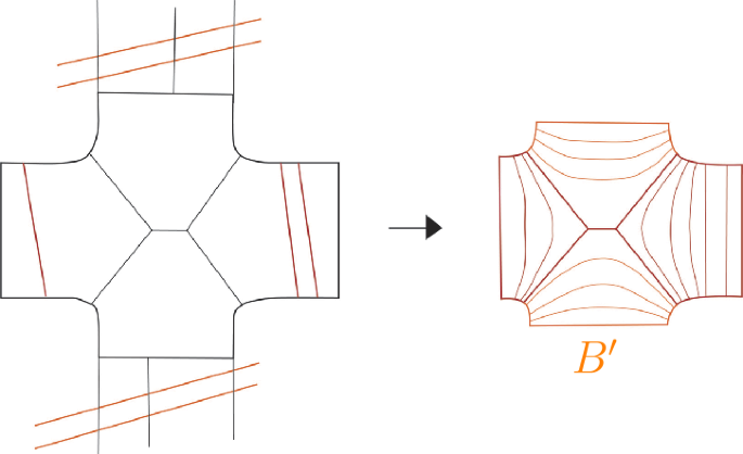

  

  After the enlargement, the disconnected branch P_Y in Fig. 12 Left becomes diffeomorphic to its corresponding branch of T_X,H.

• T_X,H changes semi-continuously in H;

• T_Y,H changes semi-continuously in H, and the realization of W on T_X,H.

Proof

The first three assertions follow from the construction of T_X,H and T_Y,H. The semi-continuity of T_X,H is given by its construction and the semi-continuity of t_X,H (Proposition 6.12). Similarly, the semi-continuity of T_Y,H follows from its construction and the semi-continuity of t_Y,H. □

6.6.2 Semi-diffeomorphic train-tracks for almost diagonal horizontal foliations

In this section, we extend the construction form §6.6.1 to the neighborhood of the diagonal (PML×PML)∖Δ^∗. By Lemma 6.4, for every compact neighborhood N of the diagonal Δ in (PML×PML)∖Δ^∗, there is δ>0, such that

$$ \angle _{E_{X, H_{X}}} ([V_{Y}]_{X}, H_{X}) > \delta $$

for all (H_X,H_Y)∈N, where V_Y is the vertical measured foliation of the flat surface structure on Y with the horizontal foliation H_Y. Let ${\mathbf{t}}_{X, H_{X}}^{r} (= {\mathbf{t}}_{X, H_{X}})$ be the train-track decomposition of $E_{X, H_{X}}$ obtained in §6.3. Lemma 6.7 clearly implies the following.

Proposition 6.20

For a compact subset N in (PML×PML)∖Δ^∗, if the train-track parameter r>0 is sufficiently small, then for all (H_X,H_Y)∈N, ${\mathbf{t}}_{X, H_{X}}^{r}$ essentially carries [V_Y]_X.

Let W_Y be a realization of [V_Y]_X on ${\mathbf{t}}_{X, H_{X}}$ by a homotopy along horizontal leaf H_X (§6.3). For every branch B_X of ${\mathbf{t}}_{X, H_{X}}$, consider the subset of $E_{Y, H_{Y}}$ which maps to W_Y|B_X by the straightening map $\operatorname{st}\colon E_{Y, H_{Y}} \to E_{X, H_{X}}$ (§6.1) and the horizontal homotopy. Then, the boundary of the subset consists of straight segments in the vertical foliation V_Y and curves topologically transversal to V_Y (Fig. 16 for the case when B_X is a rectangle). We straighten each non-vertical boundary curve of the subset keeping its endpoints (Fig. 16). let B_Y be the region in $E_{Y, H_{Y}}$ after straightening all non-vertical curves, so that the boundary of B_Y consists of segments parallel to V_Y and segments transversal to V_Y. Then, for different branches B_X of ${\mathbf{t}}_{X, H_{X}}$, corresponding regions B_Y have disjoint interiors; thus the regions B_Y yield a trapezoidal surface train-track decomposition of $E_{Y, H_{Y}}$.

Figure 16

The construction of the branch B_Y corresponding to the branch B_X by straightening of horizontal edges of the inverse image.

Let E be a flat surface, and let H be its horizontal foliation. Then, for ϵ>0, a piecewise-smooth curve c on E is ϵ-almost horizontal, if ∠_E(H,c)<ϵ, i.e. the angles between the tangent vectors along c and the foliation H are less than ϵ. More generally, c is ϵ-quasi horizontal if c is ϵ-Hausdorff close to a geodesic segment which is ϵ-almost horizontal to the horizontal foliation H. (In particular, the length of c is very short, then it is ϵ-quasi horizontal.)

Definition 6.21

Let E be a flat surface. For ϵ>0, an ϵ-quasi-staircase train-track structure of E is a trapezoidal train-track structure of E such that its horizontal edges are all ϵ-quasi horizontal straight segments.

If H_X=H_Y, then t_Y,H is a staircase train-track, by continuity, we have the following.

Lemma 6.22

Let r>0 be a train-track parameter given by Proposition 6.20. Then, for every ϵ>0, if the neighborhood N of the diagonal in PML×PML is sufficiently small, then, for all (H_X,H_Y)∈N, the trapezoidal train-track decomposition ${\mathbf{t}}_{Y, H_{Y}}^{r}$ of $E_{Y, H_{Y}}$ is ϵ-quasi staircase.

Next, similarly to §6.6.1, we modify ${\mathbf{t}}_{X, H_{X}}$ and ${\mathbf{t}}_{Y, H_{Y}}$ by gluing some branches, so that corresponding branches have small diffeomorphic neighborhoods. Let W_Y be a realization of [V_Y]_X in ${\mathbf{t}}_{X, H_{X}}$. Fix small δ>0. Let v be a vertical edge v of ${\mathbf{t}}_{X, H_{X}}$, and let B₁, B₂ be the branches of ${\mathbf{t}}_{X, H_{X}}$ whose boundary contains v. We glue B₁ and B₂ along v, if the W_Y-measure of v in B_i is less than δ for both i=1,2. By applying such gluing for all vertical edges satisfying the condition, we obtain a staircase train-track $T_{X, H_{X}}^{r, \delta } = T_{X, H_{X}}$, so that ${\mathbf{t}}_{X, H_{X}}$ is a refinement of $T_{X, H_{X}}$.

Then, W_Y is still carried by $T_{X, H_{X}}$. Therefore, let $T_{Y, H_{X}}$ be the trapezoidal train-track decomposition of $E_{Y, H_{Y}}$ obtained by this realization, so that ${\mathbf{t}}_{Y, H_{Y}}$ is its refinement.

Let v be a vertical edge of $T_{X, H_{X}}$. Let B_X be a branch of $T_{X, H_{X}}$ whose boundary contains v. Let $B_{X}'$ be the branch of $T_{X, H_{X}}$ adjacent to B_X across v. Let B_Y and $B_{Y}'$ be the branches of $T_{Y, H_{Y}}$ corresponding to B_X and $B_{X}'$, respectively. Then, there is a vertical edge w of $T_{Y, H_{Y}}$ corresponding to v, contained in the boundary of both B_Y and $B_{Y}'$.

If the W_Y-weight of v in B_X is less than δ, then the W_Y-weight of V in $B_{X}'$ is at least δ, by the construction of $T_{X, H_{X}}$. Therefore, $B_{Y}'$ contains an ϵ-quasi-staircase trapezoid R_Y, such that w is a vertical edge of R_Y and the horizontal length between the vertical edges is δ/3. (c.f. Figure 14.)

Then, we can modify the train track $T_{Y, H_{Y}}$ by removing R_Y from $B_{Y}'$ and gluing R_Y with B_Y along w — this modified $T_{Y, H_{Y}}$ by a homotopy. By simultaneously applying this modification for all vertical edges v of $T_{X, H_{X}}$ satisfying the condition, we obtain a trapezoidal train-track decomposition $T_{Y, H_{Y}}'$.

Proposition 6.23

For an arbitrary compact neighborhood N of the diagonal Δ in (PML×PML)∖Δ^∗, fix a sufficiently small train-track parameter r>0 obtained by Proposition 6.20. Then, if the parameter δ>0 is sufficiently small, then for every (H_X,H_Y)∈N,

• $T_{X, H_{X}}$ is semi-diffeomorphic to $T_{Y, H_{Y}}'$;

• $T'_{Y, H_{Y}}$ is δ-Hausdorff close to $T_{Y, H_{Y}}$ in the normalized metric $E^{1}_{Y, H_{Y}}$;

• the open δ/4-neighborhood of the singular set is disjoint from the one-skeleton of $T'_{Y, H_{Y}}$

(Fig. 17).

Figure 17

Relations between constructed train tracks.

A sliding is an operation of a train-track moving some vertical edges in the horizontal direction without changing the homotopy type of the train-track structure. If we change the realization W_Y on t_X,H by shifting across a vertical slit, the induced train-track t_Y,H changes by sliding its corresponding vertical segment (Fig. 18).

Figure 18

A slide corresponding a shift in Fig. 11.

As before, a branch of $T_{X, H_{X}}$ disjoint from the non-transversal graph G_Y is called a transversal branch. A branch of $T_{X, H_{X}}$ containing a component of G_Y is called the non-transversal branch. By the semi-continuity of $T_{Y, H_{Y}}$ in Lemma 6.19 and the construction of $T'_{Y, H_{Y}}$, we obtain a semi-continuity of $T_{Y, H_{Y}}$ up to sliding.

Lemma 6.24

Let H_i=(H_X,i,H_Y,i) be a sequence converging to H=(H_X,H_Y). Then, up to a subsequence, $T_{Y, H_{Y, i}}$ semi-converges to a train track structure $T_{Y, H_{Y}}''$ of $E_{Y, H_{Y}}$, such that either $T_{Y, H_{Y}}'' = T_{Y, H_{Y}}'$ or $T_{Y, H_{Y}}''$ can be transformed to a refinement of $T_{Y, H_{Y}}'$ by sliding some vertical edges by δ/3.

6.7 Bounded polygonal train tracks for the Riemann surface X

The train tracks we constructed may so far have rectangular branches with very long horizontal edges. In this section, we further modify the train-track structures $T_{X, H_{X}}$ and $T_{Y, H_{Y}}$ from §6.6 by reshaping those long rectangles into spiral cylinders.

Given a rectangular branch of a train track, although its interior is embedded in a flat surface, its boundary may intersect itself. Let T be a train-track structure of a flat surface E. The diameter of a branch B of T is the diameter of the interior of B with the path metric in B. The diameter of a train track T is the maximum of the diameters of the branches of T.

Recall that we have fixed a compact neighborhood N⊂(PML×PML)∖Δ^∗ of the diagonal. Recall that, for (H_X,H_Y)∈N, $E_{X, H_{X}}^{1}$ and $E_{Y, H_{Y}}^{1}$ are the unit-area flat structures realizing (X,H_X) and (Y,H_Y), respectively. Pick a small r>0 given by Proposition 6.12, so that, for every (H_X,H_Y)∈N, there are train-track structures $T_{X, H_{X}}$ of $E_{X, H_{X}}^{1}$ and $T_{Y, H_{Y}}$ of $E_{Y, H_{Y}}^{1}$ from §6.6.2.

Lemma 6.25

• (1) Let H_i=(H_X,i,H_Y,i)∈N be a sequence converging to H=(H_X,H_Y)∈N. Suppose that $T_{X, H_{X, i}} =: T_{X, i}$ contains a rectangular branch R_i for every i, such that the horizontal length of R_i diverges to infinity as i→∞. Then, up to a subsequence, the support $|R_{i}| \subset E_{X, H_{X, i}}^{1} =: E_{X, i}$ converges to either

  • a flat cylinder which is a branch of $T_{X, H_{X}}$ or

  • a closed leaf of H_X which is contained in the union of the horizontal edges of $T_{X, H_{X}}$.

• (2) Let A be the limit flat cylinder or a loop in (1). For sufficiently large i>0, let $R_{i, 1}, \dots , R_{i, n_{i}}$ be the set of all rectangular branches of T_X,i which converge to A as i→∞ in the Hausdorff metric. Then, the union $R_{i, 1} \cup \cdots \cup R_{i, n_{i}} \subset E_{X, H_{i}}^{1}$ is a spiral cylinder for all sufficiently large i. (See Fig. 7.)

Proof

(1) Let R_i be a rectangular branch of T_X,i such that the horizontal length of R_i diverges to infinity as i→∞. Then, as Area E_i=1, the vertical length of R_i must limit to zero. Then, in the universal cover $\tilde{E}_{i}$ of E_i, we can pick a lift $\tilde{R}_{i}$ of R_i which converges, uniformly on compact, to a smooth horizontal leaf of $\tilde{H}_{X}$ or a copy of $\mathbb{R}$ contained in a singular leaf of $\tilde{H}_{X}$. Let $\tilde{\ell}$ denote the limit, and let ℓ be its projection into a leaf of H_X.

Claim 6.26

ℓ is a closed leaf of H_X.

Proof

Suppose, to the contrary, that ℓ is not periodic. Then ℓ is either a leaf of an irrational sublamination or a line embedded in a singular leaf of $H_{X, H_{X}}$. Then, the distance from ℓ to the singular set of $E_{X, H_{X}}$ is zero.

Recall that the $(r, \sqrt[4]{r})$-neighborhood of the singular set of $E_{X, H_{X, i}}$ is contained in the (non-rectangular) branches of $T_{X, H_{X, i}}$. Thus, the distance from R_i to the singular set of $E_{X, H_{X,i}}$ is at least r>0 for all i. This yields a contradiction. □

By Claim 6.26, as a subset of E_i, the rectangular branch R_i converges to the union of closed leaves {ℓ_j}_j∈J of $H_{X, L_{X}}$. Thus the Hausdorff limit A of R_i in E_X,H must be a connected subset foliated by closed horizontal leaves. Therefore, A is either a flat cylinder or a single closed leaf.

First, suppose that the limit A is a flat cylinder. Then, the vertical edges of R_i are contained in the vertical edges of non-rectangular branches. The limit of the vertical edges of R_i are points on the different boundary components of A. Therefore, each boundary component of A must intersect a non-rectangular branch in its horizontal edge. Therefore, the cylinder is a branch of T_X,H by the construction of t_X,H.

If the limit A is a single leaf, similarly, one can show that the vertical one-skeleton of $T_{X, H_{X}}$, since a loop can be regarded as a degeneration of a flat cylinder.

(2) First assume that the limit A is a flat cylinder. Since the $(r, \sqrt[4]{r})$-neighborhood of the singular set is disjoint from the interior of A, we can enlarge A to a maximal flat cylinder $\hat{A}$ in E_X,H whose interior contains (the closure of) A. Then, each boundary component of $\hat{A}$ contains at least one singular point. Since A is a cylindrical branch, each boundary component ℓ of A contains a horizontal edge of a non-rectangular branch P_ℓ of $T_{X, H_{X}}$ which contains a singular point in the boundary of $\hat{A}$.

Let P_ℓ,1,…,P_ℓ,n be the non-rectangular branches of $T_{X, H_{X}}$ whose boundary intersects ℓ. Recall that P_ℓ,i is the union of some branches of t_X,H. Although $P_{\ell _{1}, i}$ itself may not be convex, a small neighborhood of the intersection P_ℓ,i∩ℓ in P_ℓ,i is convex. Let $P_{i, 1}, \dots , P_{i, k_{i}}$ be all non-rectangular branches of T_X,i, such that their union $P_{i, 1} \cup \cdots \cup P_{i, k_{i}}$ converges to the union of all non-rectangular branches of $T_{X, H_{X}}$ which have horizontal edges contained in the boundary of A. Then, for sufficiently, large i, the vertical edges of $R_{i,1}. \dots , R_{i, n_{i}}$ are contained in vertical edges of polygonal branches $P_{i, 1}, \dots , P_{i, k_{i}}$. Then, by the convexity above, if the union of $R_{i,1}, \dots , R_{i, n_{i}}$ intersects P_i,j, then its intersection is a monotone staircase curve. Therefore the union of $R_{i,1}. \dots , R_{i, n_{i}}$ is a spiral cylinder. See Fig. 19. A similar argument holds in the case when the limit is a closed loop in a singular leaf. By Lemma 6.25 (1), (2), there is a constant c>0, such that, for H_X∈N, if a rectangular branch R of $T_{X, H_{X}}$ has a horizontal edge of length more than c, then R is contained in a unique spiral cylinder, which may contain other rectangular branches. The diameter of such spiral cylinders is uniformly bounded from above by a constant depending only on X. Thus, replace all rectangular branches R of $T_{X, H_{X}}$ with corresponding spiral cylinders, and we obtain a staircase train track $\mathbf{T}_{X, H_{X}}$:

Figure 19

The spiral cylinder $\cup_{j = 1}^{n_{i}} R_{i, j}$ limiting to the flat cylinder A as i→∞.

Corollary 6.27

There is c>0, such that, for all H=(H_X,H_Y)∈N, the diameters of the branches of the staircase train track $\mathbf{T}_{X, H_{X}}$ are bounded by c.

6.8 Semi-diffeomorphic bounded almost polygonal train-track structures for Y

For ϵ>0, we have constructed, for all H=(H_X,H_Y) in some compact neighborhood N of the diagonal Λ_∞ in (PML×PML)∖Δ^∗, a staircase train-track structure $T_{X, H_{X}}$ of $E_{X, H_{X}}$ and an ϵ-quasi-staircase train-track structure $T_{Y, H_{Y}}$ of E_Y,H, such that $T_{X, H_{X}}$ is semi-diffeomorphic to $T_{Y, H_{Y}}$. In §6.7, we modify $T_{X, H_{X}}$ and obtain a uniformly bounded train-track $\mathbf{T}_{X, H_{X}}$ creating spiral cylinders. In this section, we accordingly modify $T_{Y, H_{Y}}$ to a bounded ϵ-quasi-staircase train-track structure.

Lemma 6.28

• (1) For every spiral cylinder A of $\mathbf{T}_{X, H_{X}}$, letting R_X,1,R_X,2,…,R_X,n be the rectangular branches of T_X,H whose union is A, there are corresponding branches R_Y,1,R_Y,2,…,R_Y,n of T_Y,H, such that

  • their union R_Y,1∪R_Y,2∪⋯∪R_Y,n is a spiral cylinder in $E_{Y, H_{Y}}$, and

  • A is semi-diffeomorphic to R_Y,1∪R_Y,2∪⋯∪R_Y,n.

• (2) Moreover, there is a constant c′>0, such that, if a rectangular branch of $T_{Y, H_{Y}}$ has horizontal length more than c′, then it is contained in a spiral cylinder as above.

Proof

As (H_X,H_Y)∩Δ^∗=∅, the geodesic representative [V_Y]_X essentially intersects A. Thus, the realization W_Y has positive weights on R_X,1,R_X,2,…,R_X,n. Thus R_X,j corresponds to a rectangular branch R_Y,j of $T_{Y, H_{Y}}$, and their union ∪_jR_Y,j is a spiral cylinder in $T_{Y, H_{Y}}$ ((1)).

Let R_X and R_Y be corresponding rectangular branches of $T_{X, H_{X}}$ and $T_{Y, H_{Y}}$, respectively. As (H_X,H_Y) varies only in a fixed compact neighborhood of the diagonal, the horizontal length of R_X is bilipschitz close to the length of the horizontal length of R_Y with a uniform bilipschitz constant for such all R_X and R_Y. Therefore, there is c′>0 such that if R_Y is more than c′, then the corresponding branch R_X has length more than the constant c (right before Corollary 6.27), then R_X is contained in a unique spiral cylinder (2). □

For every spiral cylinder A of $\mathbf{T}_{X, H_{X}}$, by applying Lemma 6.28, we replace the branches R_Y,1,R_Y,2,…,R_Y,n of $T_{Y, H_{Y}}$ with the spiral cylinder R_X,1∪R_X,2∪⋯∪R_X,n of $T_{Y, H_{Y}}$. Then, we obtain an ϵ-quasi-staircase train-track decomposition $\mathbf{T}_{Y, H_{Y}}$ without long rectangles:

Proposition 6.29

For every ϵ>0, there are c>0 and a neighborhood N of the diagonal in (PML×PML)∖Δ^∗, such that, for every H=(H_X,H_Y)∈N⊂PML×PML, there is an ϵ-quasi-staircase train-track decomposition $\mathbf{T}_{Y, H_{Y}}$ of $E_{Y, H_{Y}}$, such that

• (1) $\mathbf{T}_{Y, H_{Y}}'$ is δ-Hausdorff close to $\mathbf{T}_{Y, H_{Y}}$ in $E_{Y, H}^{1}$;

• (2) the diameters of $\mathbf{T}_{Y, H_{Y}}$ and $\mathbf{T}_{Y, H_{Y}}'$ are less than c;

• (3) $\mathbf{T}_{X, H_{X}}$ is semi-diffeomorphic with $\mathbf{T}_{Y, H_{Y}}'$;

• (4) $\mathbf{T}_{Y, H_{Y}}$ changes semi-continuously in (H_X,H_Y) and the realization of [V_Y]_X on $\mathbf{T}_{X, H_{X}}$.

Proof

Assertion (2) follows from Lemma 6.28 (2). Assertion (1) follows from Proposition 6.23. Assertion (3) follows from Proposition 6.23 and Lemma 6.28 (1). Assertion (4) holds, by Lemma 6.19, since $T_{Y, H_{Y}}$ changes semi-continuously in (H_X,H_Y) and the realization W_Y of [V_Y]_X on $T_{X, H_{X}}$. □

7 Thurston laminations and vertical foliations

7.1 Model Euclidean polygons and projective circular polygons

A polygon with circular boundary is a projective structure on a polygon such that the development of each edge is contained in a round circle in ${\mathbb{C}{\mathrm{P}}}^{1}$. Let σ be an ideal hyperbolic n-gon (n≥3). Let L be a measured lamination on σ except that each boundary geodesic of σ is a leaf of weight ∞. From a view point of the Thurston parameterization, it is natural to add such weight-infinity leaves. In fact, there is a unique ${\mathbb{C}{\mathrm{P}}}^{1}$-structure $\mathcal{C}= \mathcal{C}(\sigma , L)$ on the complex plane $\mathbb{C}$ whose Thurston’s parametrization is the pair (σ,L); see [GM21]. Let $\mathcal{L}$ be the Thurston lamination on $\mathcal{C}$. Denote, by $\kappa \colon \mathcal{C}\to \sigma$, the collapsing map (§2.1.7).

For each boundary edge l of σ, pick a leaf ℓ of $\mathcal{L}$ which is sent diffeomorphically onto l by κ. Then, those circular leaves bound a circular projective n-gon $\mathcal{P}$ in $\mathcal{C}$, called an ideal projective polygon.

For each i=1,2,…,n, let v_i be an ideal vertex of σ, and let l_i and l_i+1 be the edges of σ starting from v_i. Consider the geodesic g starting from v_i in the middle of l_i and l_i+1, so that the reflection about g exchanges l_i and l_i+1. Embed σ isometrically into a totally geodesic plane in $\mathbb{H}^{3}$. Accordingly $\mathcal{P}$ is embedding in ${\mathbb{C}{\mathrm{P}}}^{1}$ so that the restriction of κ to $\mathcal{P}$ is the nearest point projection to σ in $\mathbb{H}^{3}$.

Then, pick a round circle c_i on ${\mathbb{C}{\mathrm{P}}}^{1}$ such that the hyperbolic plane, Conv c_i, bounded by c_i is orthogonal to g, so that l_i and l_i+1 are transversal to Conv c_i.

Let ℓ_i and ℓ_i be the edges of $\mathcal{P}$ corresponding to l_i and l_i+1, respectively. If c_i is close to v_i enough, then there is a unique arc a_i in $\mathcal{P}$ connecting ℓ_i to ℓ_i+1 which is immersed into c_i by the developing map. Then, the region in $\mathcal{P}$ bounded by a₁…a_n is called the truncated ideal projective polygon.

Definition 7.1

Let C be a ${\mathbb{C}{\mathrm{P}}}^{1}$-structure on S. Let E¹ be the normalized flat surface of the Schwarzian parametrization of C. Let P be a staircase polygon in E¹. Then P is ϵ-close to a truncated ideal projective polygon $\mathcal{P}$, if $\mathcal{P}$ isomorphically embeds onto a polygon in C which is ϵ-Hausdorff close to P in the normalized Euclidean metric.

For X∈T⊔T^∗, recall that be the holonomy variety of the ${\mathbb{C}{\mathrm{P}}}^{1}$-structures on X. For , let C_X,ρ be the ${\mathbb{C}{\mathrm{P}}}^{1}$-structure on X with holonomy ρ, and let E_X,ρ be the flat surface given by the holomorphic quadratic differential of C_X,ρ. Similarly, for ϵ>0, let $N_{\epsilon }^{1} Z_{X, \rho}$ be the ϵ-neighborhood of the singular set in the normalized flat surface $E^{1}_{X, \rho}$. Let $\mathcal{L}_{X, \rho}$ be the Thurston lamination of C_X,ρ.

Then, by combining what we have proved, we obtain the following.

Theorem 7.2

Let X∈T⊔T^∗. Then, for every ϵ>0, there is a bounded subset K=K(X,ϵ) of satisfying the following: Suppose that ρ is in , and that the flat surface E_X,ρ contains a staircase polygon P such that

• ∂P disjoint from $N^{1}_{\epsilon }Z_{X, \rho}$ and

• the diameter of P is less than $\frac{1}{\epsilon }$.

Then

• (1) $\mathcal{L}_{X, \rho} | P$ is (1+ϵ,ϵ)-quasi-isometric to V_X,ρ|P up to an isotopy supported on $N_{\epsilon }^{1} Z_{X, \rho} \cap P$, such that, in the normalized Euclidean metric $E^{1}_{X, \rho}$,

  • (a) on P, each leaf of V is ϵ-Hausdorff-close to a leaf of $\mathcal{L}$, and

  • (b) the transversal measure of V is ϵ-close to the transversal measure of $\mathcal{L}$ for all transversal arcs whose lengths are less than one.

• (2) In the (unnormalized) Euclidean metric, P is ϵ-close to a truncated circular polygon of the hyperbolic surface in the Thurston parameters.

Proof

The assertion (1a) follows from Lemma 4.4. The assertion (1b) is given by Proposition Theorem 4.3.

We shall prove (2). Set C_X,ρ=(τ,L)∈T×ML be the ${\mathbb{C}{\mathrm{P}}}^{1}$ structure on X with holonomy in Thurston coordinates, and let κ:C_X,ρ→τ be the collapsing map. Since sufficiently away from the zero, the developing map is well-approximated by the exponential map (Lemma 3.2).

If K is sufficiently large, then for every vertical edge v of P, the restriction $\operatorname{Ep}_{X, \rho} | v$ is a (1+ϵ)-bilipschitz embedding on the Epstein surface. Therefore, by the closeness of $\operatorname{Ep}_{X, \rho}$ and $\hat{\beta}_{X, \rho}$, κ(v) is ϵ-close to a geodesic segment s_v of length $\sqrt{2} \operatorname{length}v$. By (1b), if K is large enough, L(s_v)<ϵ.

Every horizontal edge h of P is very short on the Epstein surface (Lemma 3.1). As the developing map is approximated by the Exponential map and , it follows that, if κ(h) has length less than ϵ on τ. Therefore, the image of P on the hyperbolic surface is ϵ-close to a truncated ideal polygon (see Fig. 20.)

Figure 20

The image of a staircase polygon P by the collapsing map is almost a truncated ideal hyperbolic polygon.

7.2 Equivariant circle systems

For , we shall pick a system of a ρ-equivalent round circles on ${\mathbb{C}{\mathrm{P}}}^{1}$, which will be used to construct a circular train-track structure of C_X,ρ. Let $\tilde {\mathbf{T}}_{X, \rho}$ be the π₁(S)-invariant train-track structure on $\tilde{E}_{X, \rho}$ obtained by lifting the train-track structure T_X,ρ on E_X,ρ. Let $\operatorname{Ep}^{\ast}_{X, \rho}\colon T \tilde{E}_{X, \rho} \to T \mathbb{H}^{3}$ be the differential of $\operatorname{Ep}_{X, \rho}\colon \tilde{E}_{X, \rho} \to \mathbb{H}^{3}$.

Lemma 7.3

For every ϵ>0, there is a bounded subset K_ϵ of such that, if $\rho \colon \pi _{1}(S) \to {\mathrm{PSL}}(2, \mathbb{C})$ belongs to , then, we can assign a round circle c_h to every minimal horizontal edge h of $\tilde{\mathbf{T}}_{X, \rho}$ with the following properties:

• (1) The assignment h↦c_h is ρ-equivariant.

• (2) The hyperbolic plane bounded by c_h is ϵ-almost orthogonal to the $\operatorname{Ep}^{\ast}_{X, \rho}$-images of the vertical tangent vectors along h.

• (3) If h₁, h₂ are horizontal edges of $\tilde {\mathbf{T}}_{X, \rho}$ connected by a vertical edge v of length at least ϵ, then the round circles $c_{h_{1}}$ and $c_{h_{2}}$ are disjoint.

• (4) If h₁, h₂, h₃ are “vertically consecutive” horizontal edges, such that

  • h₁ and h₂ are connected by a vertical edge v₁ of E_X,ρ-length at least ϵ;

  • h₂ and h₃ are connected by a vertical edge v₃ of length at least ϵ;

  • h₁ and h₃ are on the different sides of h₂, i.e. the normal vectors of h₂ in the direction of v₁ and v₃ are opposite,

  then $c_{h_{1}}$ and $c_{h_{3}}$ are disjoint, and they bound a round cylinder whose interior contains $c_{h_{2}}$.

Proof

Without loss of generality, we can assume that ϵ>0 is sufficiently small. With respect to the normalized Euclidean metric $E_{X, \rho}^{1}$, the lengths of minimal horizontal edges of T_X,ρ are uniformly bounded from above by Corollary 6.27, and the distances of the horizontal edges from the singular set of $E_{X, \rho}^{1}$ are uniformly bounded from below. Then, by Lemma 3.1, for every ϵ>0, if a bounded subset K_ϵ in χ is sufficiently large, then for every minimal horizontal edge h of T_X,ρ, the vertical tangent vectors along h on E_X,ρ of unit length map to ϵ-close tangent vectors of $\mathbb{H}^{3}$.

Therefore, if K_ϵ is large enough, for each minimal horizontal edge h of $\tilde {\mathbf{T}}_{Y, \rho}$, we pick a round circle c_h, such that the assignment of c_h is holonomy equivariant and that the images of vertical tangent vectors along h are ϵ²-orthogonal to the hyperbolic plane bounded by c_h.

Then, if v is a vertical edge sharing an endpoint with h, then $\operatorname{Ep}_{X, \rho} (v)$ is ϵ²-almost orthogonal to the hyperbolic plane bounded by c_h. For every sufficiently small ϵ>0, if K>0 is sufficiently large, then the geodesic segment of length, at least, ϵ connects the hyperbolic planes bounded by $c_{h_{1}}$ and $c_{h_{2}}$, and the geodesic segment is ϵ²-almost orthogonal to both hyperbolic planes. Therefore, if ϵ>0 is sufficiently small, then, by elementary hyperbolic geometry, the hyperbolic planes are disjoint, and (3) holds. By a similar argument, (4) also holds. □

The circle system in Lemma 7.3 is not unique, but unique up to an appropriate isotopy:

Proposition 7.4

For every ϵ₁>0, there is ϵ₂>0, such that, for every given two systems of round circles {c_h} and $\{c_{h}'\}$ realizing Lemma 7.3 for ϵ₂>0, there is a one-parameter family of equivalent circles systems {c_t,h} (t∈[0,1]) realizing Lemma 7.3 for ϵ₁>0 which continuously connects {c_h} to $\{c_{h}'\}$.

Proof

The proof is left for the reader. □

7.3 Pleated surfaces are close

The following gives a measure-theoretic notion of almost parallel measured laminations.

Definition 7.5

Quasi-parallel

Let L₁, L₂ be two measured geodesic laminations on a hyperbolic surface τ. Then, L₁ and L₂ are ϵ-quasi parallel, if a leaf ℓ₁ of L₁ and a leaf ℓ₂ of L₂ intersect at a point p and ∠_p(ℓ₁,ℓ₂)>ϵ, then letting s₁ and s₂ be the unit length segments in ℓ₁ and ℓ₂ centered at p,

$$ \min ( L_{1}(s_{2}), L_{2}(s_{1}) ) < \epsilon . $$

Proposition 7.6

For every ϵ>0, if a bounded subset is sufficiently large, then L_Y,ρ is ϵ-quasi-parallel to L_X,ρ on τ_X,ρ away from the non-transversal graph G_Y.

Proof

If K is sufficiently large, $\angle _{E_{X, \rho}}(H_{X, \rho}, V_{Y, \rho}')$ is uniformly bounded from below by a positive number by Lemma 6.4. Then, the assertion follows from Lemma 3.1 and Theorem 7.2. □

In this section, we show that the pleated surfaces for C_X,ρ and C_Y,ρ are close away from the non-transversal graph. Recall that $\hat{\beta}_{X, \rho}\colon \tilde{C}_{X, \rho} \to \mathbb{H}^{3}$ denotes the composition of the collapsing map and the bending map for C_X,ρ, and similarly $\hat{\beta}_{Y, \rho}\colon \tilde{C}_{Y, \rho} \to \mathbb{H}^{3}$ denotes the composition of the collapsing map and the bending map for C_Y,ρ.

Theorem 7.7

Let X,Y∈T⊔T^∗ with X≠Y. For every ϵ>0, there is a bounded subset K_ϵ in such that, for every , there are a homotopy equivalence map ϕ:E_Y,ρ→E_Y,ρ and a semi-diffeomorphism $\psi \colon \mathbf{T}_{X, \rho} \to \mathbf{T}_{Y, \rho}'$ given by Proposition 6.29 (3) satisfying the following:

• (1) $d_{E^{1}_{Y, \rho}}(\phi (z), z) < \epsilon$;

• (2) the restriction of ϕ to $E_{Y, \rho} \setminus N^{1}_{\epsilon }Z_{Y, \rho}$ can be transformed to the identity by a homotopy along vertical leaves of E_X,ρ;

• (3) $\hat{\beta}_{X, \rho}(z)$ is ϵ-close to $\hat{\beta}_{Y, \rho} \circ \tilde{\phi}\circ \tilde{\psi }(z)$ in $\mathbb{H}^{3}$ for every point $z \in \tilde{E}_{X, \rho}$ which are not in the interior of the non-transversal branches of T_X,ρ.

Using Lemma 3.1, one can prove the following.

Lemma 7.8

Let ϵ>0 and let X∈T⊔T^∗. Then, there is a compact subset K of such that, for every , if α is a monotone staircase closed curve in E_X,ρ, such that

• the total vertical length of α is more than ϵ times the total horizontal length of α, and

• α is disjoint from the ϵ-neighborhood of the singular set in the normalized metric $E^{1}_{X, \rho}$,

then $\operatorname{Ep}_{X, \rho} \tilde{\alpha}$ is a (1+ϵ,ϵ)-quasi-geodesic with respect to the vertical length.

Lemma 7.9

Let α_X be a staircase curve carried by t_X,ρ satisfying the conditions in Lemma 7.8. Then, there is a staircase geodesic closed curve α_Y carried by $\mathbf{T}_{Y, \rho}'$ satisfying the conditions in Lemma 7.8, such that the image of α by the semi-diffeomorphism $\mathbf{T}_{X, \rho} \to \mathbf{T}_{Y, \rho}'$ is homotopic to α_Y in the train-track $\mathbf{T}_{Y, \rho}'$.

Proof

The proof is left for the reader. □

Let W_Y be a realization of [V_Y]_X on T_X,ρ (§6.3). Let x be a point of the intersection of the realization W_Y and a horizontal edge of h_X of T_X,ρ. Let y be a corresponding point of V_Y,ρ (on E_Y,ρ). Recall that r is the train-track parameter, so that, in particular, horizontal edges are distance, at least, r away from the singular set in the normalized Euclidean metric. Let v_x be a vertical segment of length r/2 on $E^{1}_{X, \rho}$ such that x is the middle point of v_x. Similarly, let v_y be the vertical segment of length r/2 on $E^{1}_{Y, \rho}$ such that y is the middle point of v_y. We normalize the Epstein surfaces for C_X,ρ and C_Y,ρ so that they are ρ-equivariant for a fixed representation $\rho \colon \pi _{1}(S) \to {\mathrm{PSL}}(2, \mathbb{C})$ (not a conjugacy class).

Proposition 7.10

Corresponding vertical edges are close in $\mathbb{H}^{3}$

For every ϵ>0, there is a compact subset K in , such that, for every , if v_X and v_Y are vertical segments of E_X,ρ and of E_Y,ρ, respectively, as above, then there is a (bi-infinite) geodesic ℓ in $\mathbb{H}^{3}$ satisfying the following:

• $\operatorname{Ep}_{X, \rho} v_{X}$ is ϵ-close to a geodesic segment α_X of ℓ in C¹-metric;

• $\operatorname{Ep}_{Y, \rho} v_{Y}$ is ϵ-close to a geodesic segment α_Y of ℓ in C¹-metric;

• if p_X and p_Y are corresponding endpoints of α_X and α_Y, then the distance between $\operatorname{Ep}_{X, \rho} p_{X}$ and $\operatorname{Ep}_{Y, \rho} p_{Y}$ is at most ϵ times the diameters of E_X,ρ and E_Y,ρ.

Proof

Then, pick a L^∞-geodesic staircase closed curves ℓ_X,1, ℓ_X,2 on E_X,ρ containing v_x such that, for i=1,2, by taking appropriate lift $\tilde{\ell}_{X, 1}$ and $\tilde{\ell}_{X, 2}$ to $\tilde{E}_{X, \rho}$,

• (1) ℓ_X,i is carried by T_X,ρ;

• (2) $\tilde{\ell}_{X, 1} \cap \tilde{\ell}_{X, 2}$ is a single staircase curve connecting singular points of $\tilde{E}_{X, \rho}$, and the projection of $\tilde{\ell}_{X, 1} \cap \tilde{\ell}_{X, 2}$ to E_X,ρ does not meet a branch of T_X,ρ more than twice;

• (3) if a branch B of $\tilde{T}_{X, H_{X}}$ intersects both $\tilde{\ell}_{X, 1}$ and $\tilde{\ell}_{X, 2}$, then B intersects $\tilde{\ell}_{X, 1} \cap \tilde{\ell}_{X, 2}$;

• (4) $\tilde{\ell}_{X, 1}$ and $\tilde{\ell}_{X, 2}$ intersect, in the normalized metric of $\tilde{E}^{1}_{X, \rho}$, the ϵ-neighborhood of the singular set only in the near the endpoints of $\tilde{\ell}_{X, 1} \cap \tilde{\ell}_{X, 2}$.

Then, there are homotopies of ℓ_X,1, ℓ_X,2 to staircase vertically-geodesic closed curves $\ell '_{X,1}$, $\ell '_{X, 2}$ carried by T_X,ρ, such that the homotopies are supported on the 2ϵ-neighborhood of the singular set of $E^{1}_{X, \rho}$ and that $\ell '_{X,1}$, $\ell '_{X, 2}$ are disjoint from the ϵ-neighborhood of the zero set. Then $\operatorname{Ep}_{X, \rho} \tilde{\ell}_{X, 1}'$ and $\operatorname{Ep}_{X, \rho} \tilde{\ell}_{X,2 }'$ are (1+ϵ,ϵ)-quasi-geodesics which are close only near the segment corresponding to $\tilde{\ell}_{X, 1} \cap \tilde{\ell}_{X, 2}$.

Pick closed geodesic staircase-curves ℓ_Y,1, ℓ_Y,2 on E_Y,ρ, such that

• ℓ_Y,i contains v_y;

• the semi-diffeomorphism T_X,ρ→T_Y,ρ takes $\ell _{X, i}'$ to a curve homotopic to ℓ_Y,i on T_Y,ρ;

• ℓ_Y,i is carried by T_Y,ρ;

• ℓ_Y,i is disjoint from $N_{\epsilon }^{1} Z_{X, \rho}$.

Let α be the geodesic such that a bounded neighborhood of α contains the quasi-geodesic $\operatorname{Ep}_{X, \rho} \tilde{\ell}_{X, i}'$. Let $\tilde{\ell}_{Y, i}$ be a lift of ℓ_Y,i to $\tilde{E}_{Y, \rho}$ corresponding to $\tilde{\ell}_{X, i}'$ (connecting the same pair of points in the ideal boundary of $\tilde{S}$).

Lemma 7.11

For every ϵ>0, if a compact subset K of is sufficiently large and υ>0 is sufficiently small, then, for all , $\operatorname{Ep}_{Y, \rho} \tilde{\ell}_{Y, i}$ is (1+ϵ,ϵ)-quasi-isometric with respect to the vertical length for both i=1,2.

Then $\operatorname{Ep}_{X, \rho} \tilde{\ell}_{X, 1}' \cup \tilde{\ell}_{X, 2}'$ and $\operatorname{Ep}_{Y, \rho} \tilde{\ell}_{Y, 1} \cup \tilde{\ell}_{Y, 2}$ are both ϵ-close in the Hausdorff metric of $\mathbb{H}^{3}$. Therefore, corresponding endpoints of $\operatorname{Ep}_{Y, \rho} \tilde{\ell}_{X, 1}' \cap \tilde{\ell}_{X, 2}'$ and $\operatorname{Ep}_{Y, \rho} \tilde{\ell}_{Y, 1}' \cap \tilde{\ell}_{Y, 2}'$ have distance, at most, ϵ times the diameters of E_X,ρ and E_Y,ρ. By (2), the length of $\tilde{\ell}_{X, 1}' \cap \tilde{\ell}_{X, 2}'$ can not be too long relative to the diameter of E_X,ρ. Letting ℓ be the geodesic in $\mathbb{H}^{3}$ fellow-traveling with $\operatorname{Ep}_{X, \rho} \tilde{\ell}_{X, 1}'$ (or $\operatorname{Ep}_{X, \rho} \tilde{\ell}_{X, 2}'$), the vertical segment v_x and v_y have the desired property.  □

Finally Theorem 7.7 follows from the next proposition.

Proposition 7.12

Suppose that a branch $B_{Y}'$ of the train track $\mathbf{T}_{Y, \rho}'$ corresponds transversally to a branch B_X of T_X,ρ.

Then, there is an ϵ-small isotopy of $B_{Y}'$ in the normalized surface $E_{Y, \rho}^{1}$ such that

• in the complement of the $\frac{r}{2}$-neighborhood of the zero set, every point of $B_{Y}'$ moves along the vertical foliation V_Y,ρ, and

• after the isotopy $\hat{\beta}_{X, \rho} | B_{X}$ and $\hat{\beta}_{Y, \rho} \vert B_{Y}'$ are ϵ-close pointwise by a diffeomorphism $\psi \colon B_{Y}' \to B_{X}$.

Proof

By Proposition 7.10, there is an ϵ-small isotopy of the boundary of $B_{Y}'$ satisfying the conditions on the boundaries of the branches. Since the branches are transversal, by Theorem 4.3, if K is sufficiently large, then the restriction of L_X,ρ to B_X and L_Y,ρ on B_Y are ϵ-quasi parallel on the hyperbolic surface τ_X,ρ (Proposition 7.6). Therefore we can extend to the interior of the branch by taking an appropriate diffeomorphism $\psi \colon B'_{Y} \to B_{X}$. □

8 Compatible circular train-tracks

In §6, for every ρ in outside a large compact K, we constructed semi-diffeomorphic train-track structures T_X,ρ and $\mathbf{T}_{Y, \rho}'$ of the flat surfaces E_X,ρ and E_Y,ρ, respectively. In this section, as E_X,ρ and E_Y,ρ are the flat structures on C_X,ρ and C_Y,ρ, using Theorem 7.7, we homotope T_X,ρ and $\mathbf{T}_{Y, \rho}'$ to make them circular in a compatible manner.

8.1 Circular rectangles

A round cylinder is a cylinder on ${\mathbb{C}{\mathrm{P}}}^{1}$ bounded by two disjoint round circles. Given a round cylinder A, the boundary components of A bound unique (totally geodesic) hyperbolic planes in $\mathbb{H}^{3}$, and there is a unique geodesic ℓ orthogonal to both hyperbolic planes. Moreover A is foliated by round circles which, in $\mathbb{H}^{3}$, bound hyperbolic planes orthogonal to ℓ — we call this foliation the horizontal foliation. In addition, A is also foliated by circular arcs which are contained in round circles bounding hyperbolic planes, in $\mathbb{H}^{3}$, containing ℓ — we call this foliation the vertical foliation. Clearly, the horizontal foliation is orthogonal to the vertical foliations of A.

Definition 8.1

Let $\mathcal{R}$ be a ${\mathbb{C}{\mathrm{P}}}^{1}$-structure on a marked rectangle R, and let $f\colon R \to {\mathbb{C}{\mathrm{P}}}^{1}$ be its developing map. Then $\mathcal{R}$ is circular if there is a round cylinder A on ${\mathbb{C}{\mathrm{P}}}^{1}$ such that

• the image of f is contained in A;

• the horizontal edges of R are immersed into different boundary circles of A;

• for each vertical edge v of R, its development f(v) is a simple arc on A transverse to the horizontal foliation.

Given a circular rectangle $\mathcal{R}$, the support of $\mathcal{R}$ consists of the round cylinder A and the simple arcs on A which are the developments of the vertical edges of $\mathcal{R}$ in Definition 8.1. We denote the support by $\operatorname{Supp}\mathcal{R}$. We can pull-back the horizontal foliation on A to a foliation on $\mathcal{R}$ by the developing map, and call it the horizontal foliation of $\mathcal{R}$.

Given projective structures $\mathcal{R}$ and $\mathcal{Q}$ on a marked rectangle R, we say that $\mathcal{P}$ and $\mathcal{Q}$ are compatible if $\operatorname{Supp}\mathcal{R}= \operatorname{Supp}\mathcal{Q}$. Let $\mathcal{R}$ be a circular rectangle, such that the both vertical edges are supported on the same arc α on a circular cylinder. Then, we say that $\mathcal{R}$ is semi-compatible with α.

8.1.1 Grafting a circular rectangle

(See [Bab10].) Let $\mathcal{R}$ be a circular ${\mathbb{C}{\mathrm{P}}}^{1}$-structure on a marked rectangle R. Let A be the round cylinder in ${\mathbb{C}{\mathrm{P}}}^{1}$ which supports $\mathcal{R}$. Pick an arc α on $\mathcal{R}$, such that α connects the horizontal edges and it is transversal to the horizontal foliation of $\mathcal{R}$. Then α is embedded into A by $\operatorname{dev}\mathcal{R}$ — we call such an arc α an admissible arc. By cutting and gluing A and $\mathcal{R}$ along α in an alternating manner, we obtain a new circular ${\mathbb{C}{\mathrm{P}}}^{1}$-structure on R whose support still is $\operatorname{Supp}\mathcal{R}$. This operation is the grafting of $\mathcal{R}$ along α, and the resulting structure on R is denoted by $\operatorname{Gr}_{\alpha }\mathcal{R}$.

One can easily show that $\operatorname{Gr}_{\alpha }\mathcal{R}$ is independent of the choice of the admissible arc α, since an isotopy of α preserving its initial conditions does not change $\operatorname{Gr}_{\alpha }\mathcal{R}$.

8.2 Circular staircase loops

Let C=(f,ρ) be a ${\mathbb{C}{\mathrm{P}}}^{1}$-structure on S. A topological staircase curve is a piecewise smooth curve, such that

• its smooth segments are labeled by “horizontal” or “vertical” alternatively along the curve, and

• at every singular point, the horizontal and vertical tangent directions are linearly independent in the tangent space.

Then, a topological staircase curve s on C is circular, if the following conditions are satisfied: Letting $\tilde{s}$ be a lift of s to $\tilde{S}$,

• every horizontal segment h of $\tilde{s}$ is immersed into a round circle in ${\mathbb{C}{\mathrm{P}}}^{1}$ by f, and

• for every vertical segment v of $\tilde{s}$, letting h₁, h₂ be the horizontal edges starting from the endpoints of v,

  • the round circles c₁, c₂ containing f(h₁) and f(h₂) are disjoint, and

  • f|v is contained in the round cylinder bounded by c₁, c₂ and, it is transverse to the horizontal foliation of the round cylinder.

8.3 Circular polygons

Let P be a marked polygon with even number of edges. Then, let e₁,e₂,…,e_2n denote its edges in the cyclic order so that the edges with odd indices are vertical edges and with even indices horizontal edges. Suppose that c₂,c₄…c_2n are round circles in ${\mathbb{C}{\mathrm{P}}}^{1}$ such that, for every $i \in \mathbb{Z}/ n \mathbb{Z}$,

• c_2i and c_2(i+1) are disjoint, and

• c_2(i−1) and c_2(i+1) are contained in the same component of ${\mathbb{C}{\mathrm{P}}}^{1} \setminus c_{2i}$.

Let $\mathcal{A}_{i}$ denote the round cylinder bounded by c_2i and c_2(i+1). A circular ${\mathbb{C}{\mathrm{P}}}^{1}$-structure $\mathcal{P}$ on P is supported on $\{c_{2i}\}_{i=1}^{n}$ if

• e_2i is immersed into the round circles of c_2i by $\operatorname{dev}\mathcal{P}$ for every i=1,…n, and

• e_2i+1 is immersed into $\mathcal{A}_{i}$ and its image is transversal to the horizontal foliation of $\mathcal{A}_{i}$ (Fig. 21) for every i=0,1,…,n−1.

  Figure 21

  

  A development of a projective polygon supported on round circles (when the developing map is injective).

Let $\mathcal{P}$ be a circular ${\mathbb{C}{\mathrm{P}}}^{1}$-structure on a polygon P supported on a circle system $\{ c_{2i}\}_{i}^{n}$. For ϵ>0, $\mathcal{P}$ is ϵ-circular, if

• for every vertical edge v_i is ϵ-parallel to the vertical foliation $\mathcal{V}$ of the support cylinder $\mathcal{A}_{i}$, and

• the total transversal measure of v given by the vertical foliation $\mathcal{V}$ is less than ϵ.

(Here, by the “total” transversal measure, we mean that if v intersects a leaf of $\mathcal{V}$ more than once, and the measure is counted with multiplicity.)

Let $\mathcal{P}_{1}$, $\mathcal{P}_{2}$ be circular ${\mathbb{C}{\mathrm{P}}}^{1}$-structures on a 2n-gon P. Then $\mathcal{P}_{1}$ and $\mathcal{P}_{2}$ are compatible if, for each i=1,…,n, $\operatorname{dev}\mathcal{P}_{1}$ and $\operatorname{dev}\mathcal{P}_{2}$ take e_2i to the same round circle and the arcs f₁(v_2i−1) and f₂(v_2i−1) are the same.

Let A be a flat cylinder with geodesic boundary; then its universal cover $\tilde{A}$ is an infinite Euclidean strip. A projective structure (f,ρ) on A is circular, if the developing map $f\colon \tilde{A} \to {\mathbb{C}{\mathrm{P}}}^{1}$ is a covering map onto a round cylinder in ${\mathbb{C}{\mathrm{P}}}^{1}$.

Next, let A be a spiral cylinder. Then each boundary component b of A is a monotone staircase loop. Let $\tilde{b}$ be the lift of b to the universal cover $\tilde{A}$. Let $\{e_{i} \}_{i \in \mathbb{Z}}$ be the segments of $\tilde{b}$ linearly indexed so that e_i with an odd index is a vertical edge and with an even index is a horizontal edge; clearly $\tilde{b} = \cup _{i \in \mathbb{Z}} e_{i}$. Then, a ${\mathbb{C}{\mathrm{P}}}^{1}$-structure (f,ρ) on A is circular, if, for each boundary staircase loop b of A and each $i \in \mathbb{Z}$,

• the horizontal edge e_2i is immersed into a round circle c_i on ${\mathbb{C}{\mathrm{P}}}^{1}$;

• c_i−1, c_i and c_i+1 are disjoint, and the round annulus bounded by c_i−1 and c_i+1 contains c_i in its interior;

• f embeds v_i in the round cylinder $\mathcal{A}_{i}$ bounded by c_i and c_i+1, and f(v_i) is transverse to the circular foliation of $\mathcal{A}_{i}$.

Two circular ${\mathbb{C}{\mathrm{P}}}^{1}$-structures $\mathcal{A}_{1} = (f_{1}, \rho _{1})$, $\mathcal{A}_{2} = (f_{2}, \rho _{2})$ on a spiral cylinder A are compatible if

• ρ₁ is equal to ρ₂ up to conjugation by an element of ${\mathrm{PSL}}(2, \mathbb{C})$ (thus we can assume ρ₁=ρ₂);

• for each boundary component h of $\tilde{A}$, f₁ and f₂ take h to the same round circle;

• for each vertical edge v of $\tilde{A}$, f₁|v=f₂|v.

More generally, let $\mathcal{F}= (f_{1}, \rho _{1})$ and $\mathcal{F}' = (f_{2}, \rho _{2})$ be two circular ${\mathbb{C}{\mathrm{P}}}^{1}$-structures on stair-case surfaces F and F′. First suppose that there is a diffeomorphism ϕ:F→F′, which takes the vertices of F bijectively to those of F′. Then $\mathcal{F}$ is compatible with $\mathcal{F}'$ if

• ρ₁ is conjugate to ρ₂ (thus we can assume that ρ₁=ρ₂);

• for every vertex p₁ of $\mathcal{F}_{1}$, the development of p₁ coincides with the development of ϕ(p₂);

• for every a horizontal edge h of $\mathcal{F}_{1}$, letting h′ be its corresponding horizontal edge of $\mathcal{F}'$, then the developments of h and h′ are contained in the same round circle;

• for every vertical edge v of $\mathcal{F}$, letting v′ be its corresponding edge v′ of $\mathcal{F}'$, then the developments of v′ and v coincide.

Next, instead of a diffeomorphism, we suppose that there is a semi-diffeomorphism ϕ:F→F′. Then $\mathcal{F}$ is semi-compatible with $\mathcal{F}'$ if

• ρ₁ is conjugate to ρ₂ (thus we can assume that ρ₁=ρ₂);

• for every vertex p₁ of $\mathcal{F}_{1}$, the development of p₁ coincides with the development of ϕ(p₂);

• if a horizontal edge h of $\mathcal{F}$ corresponds to a horizontal edge h′ of $\mathcal{F}'$, then h and h′ are supported on the same round circle on ${\mathbb{C}{\mathrm{P}}}^{1}$;

• for every vertical edge v of $\mathcal{F}$, letting v′ be its corresponding vertical edge (segment) of $\mathcal{F}'$, then the developments of v′ and v coincide.

8.4 Construction of circular train tracks $\mathcal{T}_{Y,\rho}$

In this section, if ρ is in minus a large compact subset, we construct a circular train-track structure of C_Y,ρ related to the polygonal train-track decomposition $\mathbf{T}'_{Y, \rho}$.

Two train-track structures T₁, T₂ on a flat surface E is (p,q)-quasi-isometric for p>1 and q>0 if there is a continuous (p,q)-quasi-isometry ϕ:E→E homotopic to the identity such that ϕ(T₁)=T₂ and the restriction of ϕ to T₁ is a homotopy equivalence between T₁ and T₂.

Theorem 8.2

For every ϵ>0, there is a bounded subset K=K_ϵ in , such that, for every , there is an ϵ-circular surface train track decomposition $\mathcal{T}_{Y, \rho}$ of C_Y,ρ with the following properties:

• (1) $\mathcal{T}_{Y, \rho}$ is diffeomorphic to $\mathbf{T}_{Y, \rho}'$, and it is (1+ϵ,ϵ)-quasi-isometric to both T_Y,ρ and $\mathbf{T}_{Y, \rho}'$ in the normalized metric $E^{1}_{Y, \rho}$.

• (2) For every vertical edge v of $\mathbf{T}_{Y, \rho}'$, its corresponding edge of $\mathcal{T}_{Y, \rho}$ is contained in the leaf of the vertical foliation V_Y,ρ.

• (3) For a branch B_X of T_X,ρ, letting B_Y be its corresponding branch of $\mathbf{T}_{Y, \rho}'$ and letting $\mathcal{B}_{Y}$ be the branch of $\mathcal{T}_{Y, \rho}$ corresponding to B_Y, the restriction of $\hat{\beta}_{X, \rho}$ to $\partial \tilde{B}_{X}$ is ϵ-close to the restriction of $\hat{\beta}_{Y, \rho}$ to $\partial \tilde {\mathcal{B}}_{Y}$ pointwise; moreover, if B_X is a transversal branch, then $\hat{\beta}_{X, \rho} | \tilde{B}_{X}$ is ϵ-close to $\hat{\beta}_{Y, \rho} | \tilde {\mathcal{B}}_{Y}$ pointwise.

We fix a metric on the unit tangent bundle of $\mathbb{H}^{3}$ which is left-invariant under ${\mathrm{PSL}}(2, \mathbb{C})$.

Proposition 8.3

For every ϵ>0, if a bounded subset K_ϵ of is sufficiently large, then, for every and every horizontal edge h of T_X,ρ, the $\operatorname{Ep}^{\ast}_{X, \rho}$-images of the vertical unit tangent vectors of along h are ϵ-close.

Proof

The assertion immediately follows from Theorem 3.9 (2). □

Recall that we have constructed a system of equivariant circles for horizontal edges of $\tilde {\mathbf{T}}_{X, \rho}$ in Lemma 7.3. Let h=[u,w] denote the horizontal edge of T_X,ρ where u, w are the endpoints. We shall perturb the endpoints of each horizontal edge of T_Y,ρ so that the endpoints map to the corresponding round circle.

Proposition 8.4

For every ϵ>0, there are sufficiently small δ>0 and a (large) bounded subset K_ϵ of satisfying the following: For every , if c={c_h} is a circle system for horizontal edges h of T_X,ρ given by Lemma 7.3 for δ, then, for every horizontal edge h=[u,w] of $\tilde {\mathbf{T}}_{Y, \rho}$, there are, with respect to the normalized metric $E_{Y, \rho}^{1}$, ϵ-small perturbations u′ and w′ of u and w along V_Y,ρ, respectively, such that f_Y,ρ(u′) and f_Y,ρ(w′) are contained in the round circle c_h.

Proof

This follows from Theorem 7.7 and Lemma 7.3 (2). □

Proof of Theorem 8.2

By Proposition 8.4, for each horizontal edge h=[u,w] of $\mathbf{T}_{Y, \rho}'$, there is an ϵ-homotopy of h to the circular segment h′ the perturbations u′, w′ such that, letting $\tilde{h}$ be a lift of h to $\tilde{E}_{Y, \rho}$, the corresponding lift $\tilde{h}'$ of h′ is immersed into the round circle $c_{\tilde{h}}$. For each vertical edge v of $\mathbf{T}_{Y, \rho}'$, at each endpoint of v, there is a horizontal edge of $\mathbf{T}_{Y, \rho}'$ starting from the point; then the round circles corresponding to the horizontal edges bound a round cylinder.

Note that a vertex u of $\mathbf{T}_{Y, \rho}'$ is often an endpoint of different horizontal edges h₁ and h₂. Thus, if the perturbations $u_{1}'$ and $u_{2}'$ of u are different for h₁ and h₂, then $\mathcal{T}_{Y, \rho}$ has a new short vertical edge connecting $u_{1}'$ and $u_{2}'$, and $\mathcal{T}_{Y, \rho}$ is non-diffeomorphic to $\mathbf{T}_{Y, \rho}'$.

Recall that the δ/4-neighborhood of the singular points of $E_{Y, \rho}^{1}$ is disjoint from the one-skeleton of T_Y,ρ by Proposition 6.23. Thus, every vertical edge v of $\mathbf{T}_{Y, \rho}'$ is ϵ-circular with respect to the round cylinder by Corollary 3.7. Thus we have (2). Thus we obtained an ϵ-circular train-track decomposition $\mathcal{T}_{Y, \rho}$ of E_Y,ρ.

As the applies homotopies are ϵ-small, $\mathcal{T}_{Y, \rho}$ are ϵ-close to $\mathbf{T}_{Y, \rho}'$ (1). Thus we may, in addition, assume that $\mathcal{T}_{Y, \rho}$ is ϵ-close to $\mathbf{T}_{Y, \rho}'$ by Proposition 6.23. Moreover, Theorem 7.7 give (3).

8.5 Construction of $\mathcal{T}_{X, \rho}$

Given a train-track structure on a surface, the union of the edges of its branches is a locally finite graph embedded on the surface. An edge of a train-track decomposition is an edge of the graph, which contains no vertex in its interior (whereas an edge interior of a branch may contain a vertex of the train track).

Definition 8.5

Let C, C′ be ${\mathbb{C}{\mathrm{P}}}^{1}$-structures on S with the same holonomy $\rho \colon \pi _{1}(S) \to {\mathrm{PSL}}(2, \mathbb{C})$, so that $\operatorname{dev}C$ and $\operatorname{dev}C'$ are ρ-equivariant. A circular train-track decomposition $\mathcal{T}= \cup _{i} \mathcal{B}_{i}$ of C is semi-compatible with a circular train-track decomposition $\mathcal{T}' = \cup \mathcal{B}_{j}'$ of C′ if there is a marking-preserving continuous map Θ:C→C′ such that, for each branch $\mathcal{B}$ of $\mathcal{T}$, Θ takes $\mathcal{B}$ to a branch of $\mathcal{B}'$ of $\mathcal{T}'$, and that $\mathcal{B}$ and $\mathcal{B}'$ are compatible by Θ.

Theorem 8.6

For every ϵ>0, if a bounded subset K_ϵ in is sufficiently large, then, for every , there is an ϵ-circular train track decomposition $\mathcal{T}_{X, \rho}$ of C_X,ρ, such that

• (1) $\mathcal{T}_{X, \rho}$ is semi-compatible with $\mathcal{T}_{Y, \rho}$, and

• (2) $\mathcal{T}_{X,\rho}$ additively 2π-Hausdorff-close to T_X,ρ with respect to the (unnormalized) Euclidean metric E_X,ρ: More precisely, in the vertical direction, $\mathcal{T}_{X, \rho}$ is ϵ-close to T_X,ρ, and in the horizontal direction, 2π-close in the Euclidean metric of E_X,ρ for all .

Proof

First, we transform T_X,ρ by perturbing horizontal edges so that horizontal edges are circular. Recall that, the branches of $\mathcal{T}_{Y, \rho}$ are circular with respect to a fixed system c of equivariant circles given by Lemma 7.3. Thus, the β_X,ρ-images of vertical tangent vectors along h are ϵ-close to a single vector orthogonal to the hyperbolic plane bounded by c_h. Therefore, similarly to Theorem 8.2, we can modify the train-track structure T_X,ρ so that horizontal edges are circular and ϵ-Hausdorff close to the original train-track structure in the Euclidean metric of E_X,ρ (this process may create new short vertical edges). Thus we obtained an ϵ-circular train track $\mathbf{T}_{X, \rho}'$ whose horizontal edges map to their corresponding round circles of c.

Next, we make the vertical edges compatible with $\mathcal{T}_{Y, \rho}$. Recall that $\mathbf{T}_{X, H_{X}}$ has no rectangles with short vertical edges (Lemma 5.6). Therefore, we have the following.

Lemma 8.7

For every R>0, if the bounded subset K of is sufficiently large, then, for each vertical edge of $\mathbf{T}_{X, \rho}'$, the horizontal distance to adjacent vertical edges is at least R.

Thus, by Lemma 8.7, there is enough room to move vertical edges, less than 2π, so that the train-track is compatible with $\mathcal{T}_{Y, \rho}$ along vertical edges as well.

Since T_X,ρ is semi-diffeomorphic to T_Y,ρ (Proposition 6.29 (3)), $\mathcal{T}_{X, \rho}$ is semi-compatible with $\mathcal{T}_{Y, \rho}$.

9 Grafting cocycles and intersection of holonomy varieties

In this section, given a pair of ${\mathbb{C}{\mathrm{P}}}^{1}$-structures on S with the same holonomy, we shall construct a $\mathbb{Z}$-valued cocycle under the assumption that the holonomy is outside of an appropriately large compact subset of the character variety χ. Namely, we will construct a train-track graph with compatible $\mathbb{Z}$-valued weights on the branches and its immersion into S (see [PH92] for train-track graphs). This embedding captures, in a way, the “difference” of the ${\mathbb{C}{\mathrm{P}}}^{1}$-structures sharing holonomy. If a smooth arc on S is transversal to the immersed train-track graph, then the sum of the $\mathbb{Z}$-weights at the transversal intersection points is an integer— this functional defined on transversal arcs is called a transversal cocycle. Note that this cocycle value does not change under the regular homotopy of the arc if it retains the transversality. In particular, given a simple closed curve on a surface, we first homotopy the loop so that it has a minimal geometric intersection with the immersed train-track graph, and then consider its transversal cycle with the train-track graph. In this manner, we obtain a functional on the set of homotopy classes on the simple closed curves, which we call a grafting cocycle.

Goldman showed that every ${\mathbb{C}{\mathrm{P}}}^{1}$-structure with Fuchsian holonomy $\pi _{1}(S) \to {\mathrm{PSL}}_{2}\mathbb{C}$ is obtained by grafting the hyperbolic structure with the Fuchsian holonomy along a $\mathbb{Z}$-weighted multi-loop on S ([Gol87]). The grafting cocycles that we construct in this paper can be regarded as a generalization of such weighted multiloops.

9.1 Relative degree of rectangular ${\mathbb{C}{\mathrm{P}}}^{1}$-structures

Let a<b be real numbers. Let $f, g\colon [a,b] \to \mathbb{S}^{1}$ be orientation preserving immersions or constant maps, such that f(a)=g(a) and f(b)=g(b).

Definition-Lemma 9.1

The integer ♯f⁻¹(x)−♯g⁻¹(x) is independent on $x \in \mathbb{S}^{1} \setminus \{f(a), f(b)\}$, where ♯ denotes the cardinality. We call this integer the degree of f relative to g, or simply, the relative degree, and denote it by deg(f,g).

Clearly, it is not important that f and g are defined on the same interval as long as corresponding endpoints map to the same point on $\mathbb{S}^{1}$. Moreover, the degree is additive in the following sense.

Lemma 9.2

Subdivision of relative degree

Suppose in addition that f(c)=g(c) for some c∈(a,b). Then

$$ \deg (f, g) = \deg (f |_{[a,c]}, g|_{[a,c]} ) + \deg (f|_{[a,c]}, g|_{[a,c]} ). $$

The proofs of the lemmas above are elementary. Let R, Q be circular projective structures on a marked rectangle, and suppose that R and Q are compatible: By their developing maps, corresponding horizontal edges of R and Q are immersed into the same round circle on ${\mathbb{C}{\mathrm{P}}}^{1}$, and the corresponding vertices map to the same point.

Then, the degree of R relative to Q is the degree of a horizontal edge of R relative to its corresponding horizontal edge of Q — we similarly denote the degree by $\deg (R, Q) \in \mathbb{Z}$. Although R has two horizontal edges, this degree is well-defined:

Lemma 9.3

c.f. Lemma 6.2 in [Bab15]

The degree deg(R,Q) is independent of the choice of the horizontal edge.

Proof

Let A be the round cylinder on ${{\mathbb{C}{\mathrm{P}}}}^{1}$ supporting both R and Q. Then, the horizontal foliation $\mathcal{F}_{A}$ of A by round circles c induces foliations $\mathcal{F}_{R}$ and $\mathcal{F}_{Q}$ on R and Q, respectively. Then, for each leaf c of $\mathcal{F}_{A}$, the corresponding leaves ℓ_R and ℓ_Q of $\mathcal{F}_{R}$ and $\mathcal{F}_{Q}$, respectively, are immersed into c, and the endpoints of ℓ_R and ℓ_Q on the corresponding vertical edges of R and Q map to the same point on c. The degree of ℓ_R relative to ℓ_Q is an integer, and it changes continuously in the leaves c of $\mathcal{F}_{A}$. Thus, the assertion follows immediately. □

Lemma 9.4

cf. Lemma 6.2 in [Bab15]

Let R, Q be ${\mathbb{C}{\mathrm{P}}}^{1}$-structures on a marked rectangle with $\operatorname{Supp}R = \operatorname{Supp}Q$. Then

• if deg(R,Q)>0, then R is obtained by grafting Q along an admissible arc deg(R,Q) times;

• if deg(R,Q)<0, then Q is obtained by grafting R along an admissible arc −deg(R,Q) times;

• if deg(R,Q)=0, then R is isomorphic to Q (as ${\mathbb{C}{\mathrm{P}}}^{1}$-structures).

By Lemma 9.4, the “difference” of ${\mathbb{C}{\mathrm{P}}}^{1}$-rectangles R and Q can be represented by an arc α with weight deg(R,Q) such that α sits on the base rectangle connecting the horizontal edges.

Lemma 9.5

Let R and Q be circular projective structures on a marked rectangle such that $\operatorname{Supp}R = \operatorname{Supp}Q$. Let A be the round cylinder on ${\mathbb{C}{\mathrm{P}}}^{1}$ supporting R and Q. Suppose that there are admissible arcs α_R on R and α_Q on Q which develop onto the same arc on A (transversal to the horizontal foliation), so that the arcs decompose R and Q into two circular rectangles R₁, R₂ and Q₁, Q₂, respectively and $\operatorname{Supp}R_{1} = \operatorname{Supp}Q_{1}$ and $\operatorname{Supp}R_{2} = \operatorname{Supp}Q_{2}$. Then

$$ \deg (R, Q) = \deg (R_{1}, Q_{1}) + \deg (R_{2}, Q_{2}). $$

Proof

This follows from Lemma 9.2. □

9.2 Train-track graphs for planar polygons

Let P be a L^∞-convex staircase polygon in $\mathbb{E}^{2}$, which contains no singular points. We can decompose P into finitely many rectangles P₁,P₂,…,P_n by cutting P along n−1 horizontal arcs each connecting a vertex and a point on a vertical edge. Let $\mathcal{P}$, $\mathcal{Q}$ be compatible circular projective structures on P such that the round circles supporting horizontal edges are all disjoint. The decomposition P into P₁,P₂,…P_n gives decompositions of $\mathcal{P}$ into $\mathcal{P}_{1}, \mathcal{P}_{2}, \dots , \mathcal{P}_{n}$ and $\mathcal{Q}$ into $\mathcal{Q}_{1}, \mathcal{Q}_{2}, \dots , \mathcal{Q}_{n}$ such that $\operatorname{Supp}\mathcal{P}_{i} = \operatorname{Supp}\mathcal{Q}_{i}$ for i=1,2,…,n. As in §9.1, for each i, we obtain an arc α_i connecting horizontal edges of P_i with weight $\deg (\mathcal{P}_{i}, \mathcal{Q}_{i})$. Then, by splitting and combining α₁,α₂,…,α_n appropriately, we obtain a $\mathbb{Z}$-valued train-track graph $\Gamma (\mathcal{P}, \mathcal{Q})$ on P transversal to the decomposition (Fig. 22).

Figure 22

An example of a weighted train track on an L^∞-convex polygon in $\mathbb{E}^{2}$.

9.3 Train-track graphs for cylinders

Let A_X be a cylindrical branch of T_X,ρ, and let A_Y be the corresponding cylindrical branch of T_Y,ρ.

Pick a monotone staircase curve α on A_X, such that

• (1) α connects different boundary components of A_X, and its endpoints are on horizontal edges (Fig. 23),

  Figure 23

  

  A monotone staircase curve α on a spiral cylinder.

• (2) the restriction of [V_Y,ρ]_X to A_X has a leaf disjoint from A_X.

Then [V_Y,ρ]_X is essentially carried by A_X. Then, one can easily show that the choice of α is unique through an isotopy preserving the properties.

Lemma 9.6

Suppose there are two staircase curves α₁, α₂ on A_X satisfying Conditions (1) and (2). Then, α₁ and α₂ are isotopic through staircase curves α_t satisfying Conditions (1) and (2).

In Proposition 6.7, pick a realization of [V_Y]_X on the decomposition (A_X,α_X) by a homotopy of [V_Y]_X sweeping out triangles. This induces an ϵ-almost staircase curve α_Y. Similarly to Lemma 7.3, pick a system of round circles c={c_h} corresponding to horizontal edges h of α_X so that the $\operatorname{Ep}_{X, \rho}$-images of vertical tangent vectors along h are ϵ-close to a single vector orthogonal to the hyperbolic plane bounded by c_h.

Then, as in §8.4 we can accordingly isotope the curve α_Y so that the horizontal edges are supported on their corresponding circle of c and vertical edges remain vertical— let $\alpha _{Y}^{{\mathbf{c}}}$ denote the curve after this isotopy. Then $\mathcal{A}_{Y} \setminus \alpha _{Y}^{{\mathbf{c}}}$ is a circular projective structure on a staircase polygon in $\mathbb{E}^{2}$.

Then, (similarly to Theorem 8.6), we can isotope α_X to an ϵ-almost circular staircase curve $\alpha ^{{\mathbf{c}}}_{X}$ so that

• α_X is 2π-Hausdorff close to $\alpha _{X}^{{\mathbf{c}}}$;

• the horizontal edge h of $\alpha _{X}^{{\mathbf{c}}}$ is supported on c_h;

• $\mathcal{A}_{X} \setminus \alpha _{X}^{\alpha}$ is an ϵ-almost circular staircase polygon compatible with $\mathcal{A}_{Y} \setminus \alpha _{Y}^{{\mathbf{c}}}$.

As in §9.2, $\mathcal{A}_{X} \setminus \alpha _{X}^{{\mathbf{c}}}$ and $\mathcal{A}_{Y} \setminus \alpha _{Y}^{{\mathbf{c}}}$ yield a $\mathbb{Z}$-valued weighted train track $\Gamma _{A \setminus \alpha _{X}}$ on the polygon A∖α_X such that $\Gamma _{A_{X} \setminus \alpha _{X}}$ is transversal to the horizontal foliation. Up to a homotopy preserving endpoints on the horizontal edges, the endpoints of $\Gamma _{A_{X} \setminus \alpha _{X}}$ match up along α_X as $\mathbb{Z}$-weighted arcs. Thus, we obtain a weighted train-track graph $\Gamma _{A_{X}}$ on A_X.

Consider the subset of the boundary of the circular cylinder $\mathcal{A}_{X}$ which is the union of the vertical boundary edges and the vertices of $\mathcal{T}_{X, \rho}$ contained in $\partial \mathcal{A}_{X}$. Let A be the homotopy class of arcs in $\mathcal{A}_{X}$ connecting different points in this subset. Then $[\Gamma _{A_{X}}] \colon \mathsf{A}\to \mathbb{Z}$ be the map which takes an arc to its total signed intersection number with $\Gamma _{A_{X}}$.

Then Lemma 9.6 gives a uniqueness of $[\Gamma _{A_{X}}]$:

Proposition 9.7

$[\Gamma _{A_{X}}] \colon \mathsf{A}\to \mathbb{Z}$ is independent on the choice of the staircase curve α and the realization of [V_Y]_X on $(\mathcal{A}_{X}, \alpha _{X})$.

9.4 Weighted train tracks and ${\mathbb{C}{\mathrm{P}}}^{1}$-structures with the same holonomy

In this section, we suppose that Riemann surfaces X, Y have the same orientation. Let C be the set of the homotopy classes of closed curves on S (which are not necessarily simple). Given a weighted train-track graph immersed on S, it gives a cocycle taking γ∈C to its weighted intersection number with the graph.

Theorem 9.8

For all distinct X,Y∈T, there is a bounded subset K in , such that

• (1) for each , the semi-compatible train-track decompositions $\mathcal{T}_{X, \rho}$ of C_X,ρ and $\mathcal{T}_{Y, \rho}$ of C_Y,ρ in Theorem 8.6yield a $\mathbb{Z}$-weighted train track graph Γ_ρ carried by $\mathcal{T}_{X, \rho}$ (immersed in S);

• (2) the grafting cocycle $[\Gamma _{\rho}] \colon \mathsf{C}\to \mathbb{Z}$ is independent on the choices for the construction of $\mathcal{T}_{X, \rho}$ and $\mathcal{T}_{Y, \rho}$;

• (3) $[\Gamma _{\rho}] \colon \mathsf{C}\to \mathbb{Z}$ is continuous in .

Since [Γ_ρ] takes values in $\mathbb{Z}$, the continuity immediately implies the following.

Corollary 9.9

For sufficiently large boundary subset K of , [Γ_ρ] is well-defined and constant on each connected component of .

We first construct a weighted train-track in (1). Let h_X,1…h_X,n be the horizontal edges of branches of $\mathcal{T}_{X, \rho}$.

Since $\mathcal{T}_{X, \rho}$ and $\mathcal{T}_{Y, \rho}$ are semi-compatible (Proposition 8.6), for each i=1,2,…,n, letting h_Y,i be its corresponding edge of a branch of $\mathcal{T}_{Y, \rho}$ or a vertex of $\mathcal{T}_{Y, \rho}$. Then, h_X,i and h_Y,i develop into the same round circle on ${\mathbb{C}{\mathrm{P}}}^{1}$, and their corresponding endpoints map to the same point by the semi-compatibility. Thus we have the degree of h_X,i relative to h_Y,i taking a value in $\mathbb{Z}$ (Definition 9.1) for each horizontal edge:

$$ \gamma _{\rho }\colon \{h_{X, 1}, \dots , h_{X, n}\} \to \mathbb{Z}. $$

We will construct a $\mathbb{Z}$-weighted train track Γ_ρ carried by $\mathcal{T}_{X, \rho}$ so that the intersection number with h_X,i is γ_ρ(h_X,i). The train-track graph Γ_ρ will be constructed on each branch of $\mathcal{T}_{X, \rho}$:

• For each rectangular branch R of $\mathcal{T}_{X, \rho}$, we will construct a $\mathbb{Z}$-train track graph embedded in R (Proposition 9.10).

• For each cylinder A of $\mathcal{T}_{X, \rho}$, we have obtained a $\mathbb{Z}$-weighted train track graph embedded in A (§9.3).

• For each transversal branch, we will construct a $\mathbb{Z}$-weighted train track graph embedded in the branch (Proposition 9.12).

• For each non-transversal branch of $\mathcal{T}_{X, \rho}$, we will construct a $\mathbb{Z}$-weighted train track immersed in the branch (Lemma 9.15).

9.4.1 Train tracks for rectangular branches

Given an ordered pair of compatible ${\mathbb{C}{\mathrm{P}}}^{1}$-structures on a rectangle, Lemma 9.4 gives a $\mathbb{Z}$-weighted arc connecting the horizontal edges of the rectangle. Since the horizontal edges of a rectangular branch of $\mathcal{T}_{X, \rho}$ may contain a vertex, we transform the weighted arc to a weighted train-track graph so that it matches with γ_ρ.

Proposition 9.10

For every ϵ>0, there is a bounded subset K of , such that, for every , for each rectangular branch $\mathcal{R}_{X}$ of $\mathcal{T}_{X, \rho}$, there is a $\mathbb{Z}$-weighted train track graph $\Gamma _{\rho , \mathcal{R}_{X}}$ embedded in $\mathcal{R}_{X}$ satisfying the following:

• $\Gamma _{\mathcal{R}_{X}}$ induces γ_ρ;

• $\Gamma _{\mathcal{R}_{X}}$ is transversal to the horizontal foliation on ${\mathcal{R}_{X}}$;

• each horizontal edge of $\mathcal{T}_{X, \rho}$ in $\partial \mathcal{R}_{X}$ contains, at most, one endpoint of $\Gamma _{\rho , \mathcal{R}_{X}}$;

• As cocycles, Γ_R is (1+ϵ,ϵ)-quasi-isometric to (V_X,ρ|R_X)−(V_Y,ρ|R_Y), where R_X is a branch of T_X,ρ corresponding to $\mathcal{R}_{X}$ and R_Y is the branch of $\mathbf{T}_{Y, \rho}'$ corresponding to R_X.

Proof

Since $\mathcal{R}_{X}$ and $\mathcal{R}_{Y}$ share their support, let $n = \deg (\mathcal{R}_{X}, \mathcal{R}_{Y})$ as seem in Lemma 9.4. Let h_X and h_Y be corresponding horizontal edges of $\mathcal{R}_{X}$ and $\mathcal{R}_{Y}$. Then h_X=h_X,1∪⋯∪h_X,m be the decomposition of h_X into horizontal edges of $\mathcal{T}_{X}$, and let h_Y=h_Y,1∪⋯∪h_Y,m be the corresponding decomposition into horizontal edges and vertices of $\mathcal{T}_{X}$ compatible with the semi-diffeomorphism $\mathcal{T}_{X, \rho} \to \mathcal{T}_{Y, \rho}$. Let $n_{i} \in \mathbb{Z}$ be deg(h_X,i,h_Y,i). Then, by Lemma 9.2, n=n₁+⋯+n_m. Then it is easy to construct a desired $\mathbb{Z}$-weighted train track realizing such decomposition for both pairs of corresponding horizontal edges (see Fig. 24).

Figure 24

A $\mathbb{Z}$-weight train-track graph for a rectangle. Here n=n₁+n₂+n₃=n₄+n₅. The black dots are vertices of $\mathcal{T}_{X, \rho}$.

The last assertion follows from Lemma 4.1 and Theorem 7.7. □

9.4.2 Train tracks for cylinders

For each cylindrical branch $\mathcal{A}_{X}$ of $\mathcal{T}_{X, \rho}$, in §9.3, we have constructed a train-track graph $\Gamma _{\rho , \mathcal{A}_{X}}$ on $\mathcal{A}_{X}$, representing the difference between $\mathcal{A}_{X}$ and its corresponding cylindrical branch $\mathcal{A}_{Y}$ of $\mathcal{T}_{Y, \rho}$.

Proposition 9.11

For every ϵ>0, if a bounded subset K of is sufficiently large, then, for each cylindrical branch $\mathcal{A}_{X}$ of $\mathcal{T}_{X, \rho}$, the induced cocycle $[\Gamma _{\mathcal{A}_{X}}]\colon \mathsf{A}\to \mathbb{Z}$ times 2π is (1+ϵ,ϵ)-quasi-isometric to V_Y,ρ|A_X−V_X,ρ|A_Y, where A_X and A_Y are the corresponding cylindrical branches of T_X,ρ and $\mathbf{T}_{Y, \rho}'$.

Proof

Recall that $\Gamma _{\mathcal{A}_{X}}$ is obtained from $\mathbb{Z}$-weighted train-track graphs on the rectangles. There is a uniform upper bound, which depends only on S, for the number of the rectangles used to define $[\Gamma _{\mathcal{A}_{X}}]$, since the decomposition was along horizontal arcs starting from singular points. Then, on each rectangle, the weighted graph is (1+ϵ,ϵ)-quasi-isometric to the difference of V_X,ρ and V_Y,ρ by Proposition 9.10. Thus $[\Gamma _{\mathcal{A}_{X}}]$ is also (1+ϵ,ϵ)-quasi-isometric to the difference of V_X,ρ and V_Y,ρ if K is sufficiently large. □

9.4.3 Train-track graphs for transversal polygonal branches

Recall that all transversal branches are polygonal or cylindrical (Lemma 6.18), i.e. their Euler characteristics are non-negative.

Proposition 9.12

For every ϵ>0, there is a bounded subset K in such that, for each transversal polygonal branch $\mathcal{P}_{X}$ of $\mathcal{T}_{X, \rho}$, there is a $\mathbb{Z}$-weighted train track $\Gamma _{\rho , \mathcal{P}_{X}}$ embedded in $\mathcal{P}_{X}$, letting P_X and P_Y be the branches of T_X,ρ and T_Y,ρ, respectively, corresponding to $\mathcal{P}_{X}$, respectively, such that

• (1) each horizontal edge h of $\mathcal{P}_{X}$ contains, at most, one endpoint of Γ_ρ,P;

• (2) $[\Gamma _{\mathcal{P}_{X}}]$ agrees with γ_ρ on the horizontal edges of $\mathcal{T}_{X, \rho}$ contained in $\partial \mathcal{P}_{X}$;

• (3) Γ_P is transversal to the horizontal foliation H_X,ρ on P_X;

• (4) 2π[Γ_P] is (1+ϵ,ϵ)-quasiisometric to (V_X,ρ|P_X−V_Y,ρ|P_Y).

For every ϵ>0, if K is sufficiently large, then, by Theorem 7.2, let $\hat{\mathcal{Q}}_{X}$ be an ideal circular polygon whose truncation ${\mathcal{Q}}_{X}$ is ϵ-close to $\mathcal{P}_{X}$ in C_X,ρ. Similarly, $\hat{\mathcal{Q}}_{Y}$ be an ideal circular polygon whose truncation $\mathcal{Q}_{Y}$ is ϵ-close to $\mathcal{P}_{Y}$. Since $\operatorname{Supp}\mathcal{P}_{X} = \operatorname{Supp}\mathcal{P}_{Y}$ as circular polygons, we may in addition assume that $\operatorname{Supp}\mathcal{Q}_{X} = \operatorname{Supp}\mathcal{Q}_{Y}$ as truncated idea polygons.

Let $\overline{\mathcal{Q}}_{X}$ be the canonical polynomial ${\mathbb{C}{\mathrm{P}}}^{1}$-structure on $\mathbb{C}$ which contains $\hat{\mathcal{Q}}_{X}$ (§7.1). Let $\hat{\mathcal{L}}_{X}$ be the restriction of the Thurston lamination of $\overline {\mathcal{Q}}_{X}$ to $\hat{\mathcal{Q}}_{X}$. Similarly, let $\overline{\mathcal{Q}}_{Y}$ be the canonical polynomial ${\mathbb{C}{\mathrm{P}}}^{1}$-structure on $\mathbb{C}$ which contains $\mathcal{Q}_{Y}$. Let $\hat{\mathcal{L}}_{Y}$ be the restriction of the Thurston lamination of $\overline {\mathcal{Q}}_{Y}$ to $\hat{\mathcal{Q}}_{Y}$. As $\operatorname{Supp}\mathcal{Q}_{X} = \operatorname{Supp}\mathcal{Q}_{Y}$, thus $\overline{\mathcal{Q}}_{X}$ and $\overline{\mathcal{Q}}_{Y}$ share their ideal vertices. Then $\mathcal{Q}_{X}$ and $\mathcal{Q}_{Y}$ are ϵ-close to $\mathcal{P}_{X}$ and $\mathcal{P}_{Y}$, respectively. Thus, since γ_ρ takes values in $\mathbb{Z}$, $\hat{\mathcal{L}}_{X} - \hat{\mathcal{L}}_{Y}$ satisfies (2).

Theorem 7.2 (1) implies that $\hat{\mathcal{L}}_{X}$ is (1+ϵ,ϵ)-quasi-isometric to V_X|P_X and $\hat{\mathcal{L}}_{Y}$ is (1+ϵ,ϵ)-quasi-isometric to V_Y|P_Y, and therefore $\hat{\mathcal{L}}_{X} - \hat{\mathcal{L}}_{Y}$ satisfies (4).

(1) is easy to be realized by homotopy combining the edges of the train-track graph ending on the same horizontal edge. We show that there is a $\mathbb{Z}$-weighted train track Γ which is ϵ-close to $\hat{\mathcal{L}}_{X} - \hat{\mathcal{L}}_{Y}$, satisfying (3).

Let $\Gamma _{X}^{P}$ be a weighted train track graph on P which represents $\hat{\mathcal{L}}_{X}$ a Let $\Gamma _{Y}^{P}$ be the weighted train-track graph which represents $\hat{\mathcal{L}}_{Y}$. By Theorem 7.7, the pleated surface of $\mathcal{P}_{X}$ is ϵ-close to the pleated surface of $\mathcal{P}_{Y}$, because of the quasi-parallelism in Proposition 7.6. Let $\check{\Gamma }_{X}^{P}$ be the subgraph of $|\Gamma _{X}^{P}|$ obtained by eliminating the edges of weights less than a sufficiently small ϵ. Similarly, let $\check{\Gamma }_{Y}^{P}$ be the subgraph of $\Gamma _{Y}^{P}$ obtained by eliminating the edges of weight less than ϵ.

Then, there is a minimal train-track graph Γ^P containing both $\check{\Gamma }_{Y}^{P}$ and $\check{\Gamma }_{X}^{P}$ and satisfying (1). Since the pleated surfaces are sufficiently close, by approximating the weights of $\Gamma _{X}^{P} - \Gamma _{Y}^{P}$ by integers, we obtain a desired $\mathbb{Z}$-weighted train-track graph supported on Γ^P.

Since $\mathcal{P}_{X}$ is a transversal branch, $\Gamma _{X}^{P}$ and $\Gamma _{Y}^{P}$ are both transversal to H_X,ρ|P, thus Γ^P is transversal to H_X,ρ|P (3).

9.4.4 Train-track graphs for non-transversal branches

Let P_X and P_Y be the corresponding branches of T_X,ρ and T_Y,ρ, respectively, which are non-transversal. Let $\mathcal{P}_{X}$ and $\mathcal{P}_{Y}$ be the branches of $\mathcal{T}_{X, \rho}$ and $\mathcal{T}_{Y, \rho}$ corresponding to P_X and P_Y, respectively. Then, by Theorem 8.2, $\hat{\beta}_{X, \rho} | \partial \mathcal{P}_{X}$ is ϵ-close to $\hat{\beta}_{Y, \rho} | \partial \mathcal{P}_{Y}$ in the C⁰-metric and C¹-close along the vertical edges. Let σ_X be a pleated surface with crown-shaped boundary whose truncation approximates $\hat{\beta}_{X} | \mathcal{P}_{X}$, and let σ_Y be the pleated surfaced boundary with crown-shaped boundary whose truncation approximates $\hat{\beta}_{Y} | \mathcal{P}_{Y}$, such that σ_X and σ_Y share their boundary (in $\mathbb{H}^{3}$). In particular, the base hyperbolic surfaces for σ_X and σ_Y are diffeomorphic preserving markings and spikes.

Let ν_X and ν_Y be the bending measured laminations for σ_X and σ_Y, respectively; then ν_X and ν_Y contain only finitely many leaves whose connect ideal points.

In Thurston coordinates, the developing map and the pleated surface of a ${\mathbb{C}{\mathrm{P}}}^{1}$-structure are related by the nearest point projection to the supporting planes of the pleated surface ([KP94, Bab20]). For small υ>0, let F_X, F_Y be the surfaces in $\mathbb{H}^{3}$ which are at distance υ from σ_X and σ_Y in the direction of the nearest point projections of P_X and P_Y ([EM87, Chapter II.2]).

Thus, if necessary, refining ν_X to ν_Y to ideal triangulations of the hyperbolic surfaces appropriately, pick an (irreducible) sequence of flips w_i which connects ν_X to ν_Y. Clearly the sequence w_i corresponds to a sequence of triangulations.

Lemma 9.13

If a bounded subset is sufficiently large, for every and all non-transversal branches P_X and P_Y, there is a uniform upper bound on the length of the flip sequence which depends only on X,Y∈T, or appropriate refinements into triangulations.

Proof

This follows from the length bound in Proposition 6.2. □

A triangulation in the sequence given by w_i is realizable, if there is an equivariant pleated surface homotopic to σ_X (and σ_Y) relative to the boundary such that the pleating locus agrees with the triangulation. In general, a triangulation in the sequence is not realizable when the endpoints of edges develop to the same point on ${\mathbb{C}{\mathrm{P}}}^{1}$. However a generic perturbation makes the triangulation realizable:

Lemma 9.14

For almost every perturbation of the holonomy of P_X and holonomy equivariant perturbation of the (ideal) vertices of $\tilde{\sigma }_{X}$ (and $\tilde{\sigma }_{Y}$) in ${\mathbb{C}{\mathrm{P}}}^{1}$, all triangulations in the flip sequence w_i are realizable. Moreover, the set of realizable perturbations is connected.

Proof

If σ_X is an ideal polygon, the holonomy is trivial. Then, since there are only finitely many vertices and ${\mathbb{C}{\mathrm{P}}}^{1}$ has real dimension two, almost every perturbation is realizable.

If σ_X is not a polygon, an edge of a triangulation forms a loop if the endpoints are at the same spike of τ_X. For each loop ℓ of τ_X, the condition that the holonomy of ℓ is the identity is a complex codimension, at least, one in the character variety (and also in the representation variety). Since the flip sequence is finite, for almost all perturbations of the holonomy, if an edge of a triangulation in the sequence forms a loop, then its holonomy is non-trivial. Clearly, such a perturbation is connected. Then, for every such perturbation of the holonomy, it is easy to see that, for almost all equivariant perturbations of the ideal points, the triangulations in the sequence are realizable. □

For every perturbation of the holonomy and the ideal vertices given by Lemma 9.14, the flip sequence w_i gives the sequence of pleated surfaces $\sigma _{X} = \sigma _{1} \xrightarrow{w_{1}} \sigma _{2} \xrightarrow{w_{2}} \dots \xrightarrow{w_{n-1}} \sigma _{n} = \sigma _{Y}$ in $\mathbb{H}^{3}$ connecting σ_Y to σ_X, such that σ_i’s share their boundary geodesics and ideal vertices.

For each flip w_i, the pairs of triangles of the adjacent pleated surfaces σ_i and σ_i+1 bound a tetrahedron in $\mathbb{H}^{3}$. To be precise, if the four vertices are contained in a plane, the tetrahedron is collapsed into a quadrangle, but it does not affect the following argument. The edges exchanged by the flip correspond to the opposite edges of the tetrahedron. Then pick a geodesic segment connecting those opposite edges. Then there is a path σ_t (i≤t≤i+1) of pleated surfaces with a single cone point of angle more than 2π such that

• σ_t connects σ_i to σ_i+1;

• the pleated surfaces σ share their quadrangular boundary, which corresponds to the ideal quadrangle supporting the flip w_i;

• by the homotopy, σ_t sweeps out the tetrahedron;

• the cone point on the geodesic segment (see Fig. 25).

  Figure 25

  

  The gray solid lines are the pleating lamination interpolating the pleated surfaces which differ by a flip.

In this manner, this sequence of pleated surfaces σ_i continuously extends to a homotopy of the pleated surfaces with, at most, one singular point of cone angle greater than 2π. This interpolation also connects a bending cocycle on σ_i to a bending cocycle on σ_i+1 continuous, although the induced cocycle on σ_i+1 may correspond to a measured lamination only immersed on the surface, since the edges of the triangulations transversally intersect. Thus, ν_X induces a sequence of the bending (immersed) measured laminations ν_i of σ_i supported a union of the pleating loci of σ₁,…,σ_i.

For each i, the difference ν_i+1−ν_i of the transverse cocycles is supported on the geodesics corresponding to the edges of the tetrahedron, so that, on the surface, the edges form an ideal rectangle with both diagonals. Let μ_i be the difference cocycle ν_i+1−ν_i. From each vertex of the ideal rectangle, there are three leaves of ν_i+1−ν_i starting, and the sum of their weights is zero by Euclidean geometry (Fig. 26). Note that P_X can be identified with σ_X by collapsing each horizontal edge of P_X to a point. Hence, for every i, if α is a closed curve on P_X or an arc connecting vertical edges of P_X, then μ_i(α)=0. By regarding ν_j is a geodesic lamination on σ_X, their union $\cup _{j = 1}^{i} \nu _{j}$ is a graph on σ_X whose vertices are the transversal intersection points of the triangulations. A small regular neighborhood N of $\cup _{j = 1}^{i} \nu _{j}$ is decomposed into a small regular neighborhood N₀ of the vertices and a small regular neighborhood of the edges minus N₀ in N∖N₀.

Figure 26

The link of a vertex of the ideal rectangle ----- the sum of the indicated singed angles is zero.

Since, after the Whitehead moves, the pleated surface σ_X is transformed into a pleated surface σ_Y. Thus ν_n−ν_Y gives a $\mathbb{Z}$-valued transversal cocycle.

By the construction of the regular homotopy, we have the following.

Proposition 9.15

Train tracks for non-transversal branches

For every non-transversally compatible branches $\mathcal{P}_{X}$ of $\mathcal{T}_{X, \rho}$ and $\mathcal{P}_{Y}$ of $\mathcal{T}_{Y, \rho}$, there is a $\mathbb{Z}$-weighted immersed train-track graph $\Gamma _{P_{X}}$ representing the transversal cocycle supported on $\cup _{j = 1}^{i} \nu _{j}$. Moreover, the train-track cocycle is independent of the choice of the flip sequence w_i.

Proof

Given two flip sequences (w_i), $(w_{j}')$ connecting the triangulations of σ_X to σ_Y, there are connected by a sequence of sequences $(v_{i}^{k})$ of triangulations connecting σ_X to σ_Y, such that $(v_{i}^{k})$ and $(v_{i}^{k+1})$ differ by either an involutivity, a commutativity or a pentagon relation ([Pen12, Chap. 5, Corollary 1.2]). Clearly, the difference by an involutivity and a commutativity do not affect the resulting cocycle. Also by the pentagon relation, the pleated surface does not change including the bending measure since each flip preserves the total bending along the vertices. Therefore $(v_{i}^{k})$ and $(v_{i}^{k+1})$ give the same train-track cocycle. □

Therefore we obtain $\mathsf{A}\to \mathbb{Z}$. By continuity and the connectedness in Lemma 9.14. we have the following.

Corollary 9.16

[Γ_P] is independent on the choice of the perturbation in Lemma 9.14.

There are only finitely many combinatorial types of the train-tracks T_X,ρ. We say that a branch B_X of T_X,ρ and a branch $B_{X}'$ of T_X,ρ′ are isotopic if they are diffeomorphic and isotopic on S. Then there are only finitely many isotopy classes of branches of T_X,ρ for all . Let α be an arc α on a branch B_X, such that each endpoint of α is at either on a vertical edge or a vertex of T_X,ρ.

Proposition 9.17

Let X,Y∈T. For every ϵ>0, there a compact subset K in with the following property: For every pair (B_X,α) of an isotopy class of a branch B_X and an arc α as above, there is a constant k_α>0 such that, if B_X is a (non-transversal) branch of T_X,ρ for some , then, $2\pi [\Gamma _{P_{X}}] (\alpha )$ is (1+ϵ,k_α)-quasi-isometric to $\sqrt{2}(V_{X} | P_{X} - V_{Y} | P_{Y}) (\alpha )$.

Proof

Since the length of the flip sequence is bounded from above, the difference between ν_X and ν_n is uniformly bounded in the space of transverse cocycles on S. Then the assertion follows. □

9.4.5 Independency of the transverse cocycle

From the train-track decompositions $\mathcal{T}_{X, \rho}$ and $\mathcal{T}_{Y, \rho}$, we have constructed a weighted train-track graph Γ_ρ (Theorem 9.8 (1)). Next we show its cocycle is independent on the train-track decompositions $\mathcal{T}_{X, \rho}$ and $\mathcal{T}_{Y, \rho}$ (Theorem 9.8(2)).

Recall that the train-track decompositions $\mathcal{T}_{X, \rho}$ and $\mathcal{T}_{Y, \rho}$ are determined by

• (1) the holonomy equivariant circle system c={c_h} indexed by horizontal edges h of $\tilde {\mathbf{T}}_{X, \rho}$ (given by Lemma 7.3),

• (2) the realization W_Y of [V_Y,ρ]_X,ρ on T_X,ρ (Lemma 6.7), and

• (3) the choice of vertical edges of $\mathcal{T}_{X, \rho}$ (Theorem 8.6 (2)).

Proposition 9.18

The cocycle $[\Gamma _{\rho}]\colon \mathsf{C}\to \mathbb{Z}$ constructed above is independent of the construction for $\mathcal{T}_{X, \rho}$ and $\mathcal{T}_{Y, \rho}$, i.e. (1), (2), (3).

Proof

(1) By Proposition 7.4, given two appropriate circle systems {c_h} and $\{c'_{h}\}$, there is an equivariant isotopy of circles systems {c_t,h} connecting {c_h} to $\{c'_{h}\}$. Then accordingly, we obtain a continuous family of cocycles $[\Gamma _{t, \rho}]\colon \mathsf{C}\to \mathbb{Z}$. As it takes discrete values, [Γ_t,ρ] must remain the same.

By the different choices for (2) and (3), the $\mathbb{Z}$-weights on Γ shift across bigon regions corresponding vertical edges of T_Y,ρ by integer values. These weight shifts clearly preserve the cocycle $[\Gamma _{\rho}]\colon \mathsf{C}\to \mathbb{Z}$. □

9.4.6 Continuity of the transverse cocycle

Next we prove the continuity of [Γ_ρ] in ρ claimed in (3).

Definition 9.19

Convergence and semi-convergence of train tracks

Suppose that C_i∈P converges to C∈P. In addition, suppose, for each i, there are a train-track structure $\mathcal{T}_{i}$ of C_i and a train-track structure $\mathcal{T}$ for C. Then,

• $\mathcal{T}_{i}$ converges to $\mathcal{T}$ if

  • for every branch $\mathcal{P}$ of $\mathcal{T}$, there is a sequence of branches $\mathcal{P}_{i}$ of $\mathcal{T}_{i}$ converging to $\mathcal{P}$, and

  • for every sequence of branches $\mathcal{P}_{i}$ of $\mathcal{T}_{i}$, up to a subsequence, converges to either a branch of $\mathcal{T}$ or an edge of a branch of $\mathcal{T}$.

• $\mathcal{T}_{i}$ semi-converges to $\mathcal{T}$ if there is a subdivision of $\mathcal{T}$ into another circular train-track structure $\mathcal{T}'$ so that $\mathcal{T}_{i}$ converges to $\mathcal{T}'$.

Lemma 9.20

Let ρ_i be a sequence in converging to , where K is a sufficiently large compact (as in Theorem 8.6). Pick an equivariant circle system c_i for $\mathbf{T}_{X, \rho _{i}}$ by Lemma 7.3 which converges to a circle system c for T_X,ρ. Then, up to a subsequence,

• the circular train track $\mathcal{T}_{X, \rho _{i}}$ of $C_{X, \rho _{i}}$ semi-converges to a circular train track $\mathcal{T}_{X, \rho}$ of C_X,ρ;

• the circular train track $\mathcal{T}_{Y, \rho _{i}}$ of $C_{Y, \rho _{i}}$ semi-converges to a circular train track $\mathcal{T}_{Y, \rho}$ of C_Y,ρ;

• $\mathcal{T}_{X, \rho}$ is semi-compatible with $\mathcal{T}_{Y, \rho}$.

Proof

By Lemma 6.19, $\mathbf{T}_{X, \rho _{i}}$ semi-converges to T_X,ρ. Therefore $\mathbf{T}_{X, \rho _{i}}$ converges to a subdivision $\mathbf{T}_{X, \rho}'$ of T_X,ρ as i→∞. Then, if $\mathbf{T}_{X, \rho} \neq \mathbf{T}_{X, \rho}'$, then T_X,ρ is obtained from $\mathbf{T}_{X, \rho}'$ by gluing non-rectangular branches with rectangular branches of small width or replacing long rectangles into spiral cylinders (as in §5.3 and §6.7).

Recall that 7 the realization of $[V_{Y, \rho _{i}}]_{X,\rho _{i}}$ in the train track $\mathbf{T}_{X, \rho _{i}}$ is unique up to shifting across vertical edges of non-rectangular branches (Proposition 6.12 (2)). Therefore, up to a subsequence, the realization of $[V_{Y, \rho _{i}}]_{X,\rho _{i}}$ on $\mathbf{T}_{X, \rho _{i}}$ converges to a realization of [V_Y,ρ]_X on $\mathbf{T}_{X, \rho}'$, Since $\mathbf{T}_{X, \rho}'$ is a subdivision of T_X,ρ, the limit can be regarded as also a realization on T_X,ρ. Since the realization determines the train-track structure of E_Y,ρ, up to a subsequence, $\mathbf{T}_{Y, \rho _{i}}$ converges to a bounded train-track $\mathbf{T}_{Y, \rho}'$. Then T_Y,ρ is transformed to $\mathbf{T}_{Y, \rho}'$ by possibly sliding vertical edges and subdividing spiral cylinders to wide rectangles. Moreover, by Theorem 8.2 (1), $\mathcal{T}_{Y, \rho}$ is (1+ϵ,ϵ)-quasiisometric to T_Y,ρ. Therefore, up to a subsequence, $\mathcal{T}_{Y, \rho _{i}}$ converges to a circular train-track structure $\mathcal{T}_{Y}'$ of C_Y,ρ. If $\mathcal{T}_{Y, \rho}$ is different from $\mathcal{T}_{Y, \rho}'$, then $\mathcal{T}_{Y, \rho}$ can be transformed to $\mathcal{T}_{Y, \rho}'$ by sliding vertical edges and subdividing spiral cylinders into rectangles.

By Theorem 8.6, $\mathcal{T}_{X, \rho _{i}}$ is additively 2π-close to $\mathbf{T}_{X, \rho _{i}}$ in the Hausdorff metric of $E^{1}_{X, \rho}$. Therefore, up to a subsequence $\mathcal{T}_{X, \rho _{i}}$ converges to a circular train track decomposition $\mathcal{T}_{X, \rho}'$ semi-diffeomorphic to $\mathcal{T}_{Y, \rho}$. Moreover $\mathcal{T}_{X, \rho}$ can be transformed to $\mathcal{T}_{X, \rho}'$ possibly by subdividing and sliding by 2π or 4π.

We have already shown that $\mathcal{T}_{X, \rho}$ is semi-diffeomorphic to $\mathcal{T}_{Y, \rho}$ (Theorem 8.6).

Finally we have the continuity (3).

Corollary 9.21

$[\Gamma _{\rho _{i}}]\colon \mathsf{C}\to \mathbb{Z}$ converges to $[\Gamma _{\rho}]\colon \mathsf{C}\to \mathbb{Z}$ as i→∞.

Proof

Since $\mathcal{T}_{X, \rho _{i}}$ semi-converges to $\mathcal{T}_{X, \rho}$, up to taking a subsequence, $\mathcal{T}_{X,i}$ converges to a subdivision $\mathcal{T}'_{X, \rho}$ of $\mathcal{T}_{X, \rho}$. Accordingly, there is a subdivision $\mathcal{T}'_{Y, \rho}$ of $\mathcal{T}_{Y, \rho}$, such that, to up a subsequence, $\mathcal{T}_{Y,i}$ converges to $\mathcal{T}'_{Y, \rho}$ and that $\mathcal{T}'_{X, \rho}$ is semi-diffeomorphic to $\mathcal{T}'_{Y, \rho}$.

Let $\Gamma _{\rho _{i}}$ be the $\mathbb{Z}$-weighted train-track given by $\mathcal{T}_{X, \rho _{i}}$ and $\mathcal{T}_{Y, \rho _{i}}$. Let $\Gamma _{\rho}'$ be the $\mathbb{Z}$-weighted train track given $\mathcal{T}'_{X, \rho}$ and $\mathcal{T}'_{Y, \rho}$. Then, by the convergence of the train tracks, $\Gamma _{\rho _{i}}$ converges to $\Gamma _{\rho}'$ as i→∞. Since $\mathcal{T}'_{X, \rho}$ and $\mathcal{T}'_{Y, \rho}$ are obtained by sliding and subdividing $\mathcal{T}_{X, \rho}$ and $\mathcal{T}_{Y, \rho}$ respectively, thus $\Gamma _{\rho}'$ and Γ_ρ yield the same cocycle $\mathsf{C}\to \mathbb{Z}$. □

9.5 Approximation of the grafting cocycle [Γ_ρ] by vertical foliations

Suppose that X, Y be distinct marked Riemann surfaces homeomorphic to S such that X and Y have the same orientation. For a branch B_X of T_X,ρ, let A(B_X) be the homotopy class of arcs α on $\mathcal{R}_{X}$ such that every endpoint of α is either on a vertical edge or a vertex of T_X,ρ.

Theorem 9.22

Let c₁,…,c_n be essential closed curves on S. Then, for every ϵ>0, there is a bounded subset K_ϵ of such that, for every , the grafting cocycle [Γ_ρ] times 2π is (1+ϵ,q)-quasi-isometric to $\sqrt{2} (V_{X, \rho} - V_{Y, \rho})$ along c₁,…,c_n. That is,

$$ (1 - \epsilon ) 2\pi \Gamma _{\rho }(c_{i}) - q < \sqrt{2}(V_{X, \rho}(c_{i}) - V_{Y, \rho} (c_{i}) ) < (1 + \epsilon ) 2\pi \Gamma _{\rho }(c_{i}) + q $$

(2)

for all i=1,2,…,n.

Proof

Let H∈PML. Recall that $E^{1}_{X, H}$ is the flat surface conformal to X, such that the horizontal foliation is H and AreaE¹(X,H)=1. Let T_X,H be the bounded train-track structure of E_X,H.

Then, every closed curve c can be isotoped to a closed curve c′ so that, for each branch of B of T_X,ρ, c′|B is an arc connecting different vertices. Let $c'_{1}, \dots , c'_{m}$ be the decomposition into sub-arcs. By the finiteness of possible train-tracks, the number m of the subarcs is bounded from above for all ρ. Then $2\pi \Gamma _{\rho }| c'_{j}$ is, if B is a transversal branch, (1+ϵ,ϵ)-quasi-isometric to $\sqrt{2}(V_{X, \rho} | B - V_{Y, \rho} | B) c_{k}'$ by Proposition 9.12(4), Proposition 9.11, Proposition 9.10, and, if non-transversal, (1+ϵ,q)-quasi-isometric by Proposition 9.17. As the number of subarcs is bounded, the assertion follows. □

10 The discreteness

10.1 The discreteness of the intersection of holonomy varieties

Theorem 10.1

Suppose that X, Y are marked Riemann surface structures on S with the same orientation. Then every (connected) component of is bounded.

Proof

Let K be a component of . Suppose, to the contrary, that V is unbounded in . Then, there is a path ρ_t in which leaves every compact subset. Then, by Corollary 4.6, by taking a diverging sequence t₁<t₂<⋯, there are $k_{i}, k_{i}' \in \mathbb{R}_{> 0}$ such that $\frac{k_{i}}{k_{i}'} \to 1$ as i→∞ and

$$ \lim _{i \to \infty } k_{i} H_{X, \rho _{t_{i}}} = \lim _{i \to \infty }k'_{i} H_{Y, \rho _{t_{i}}} \in \mathsf{ML}. $$

By taking a subsequence, we may, in addition, assume that their vertical foliations $[V_{X, \rho _{t_{i}}}]$ and $[V_{Y, \rho _{t_{i}}}]$ converge in PML. Thus let [V_X,∞] and [V_Y,∞] be their respective limits in PML. Since X≠Y, V_X,∞ and V_Y,∞ can not be asymptotically the same, in comparison to their horizontal foliations. Then $V_{X, \rho _{t_{i}}} - V_{Y, \rho _{t_{i}}}$ “diverges to ∞”. That is, there is a closed curve α on S, such that

$$ | V_{X, \rho _{t_{i}}}(\alpha ) - V_{Y, \rho _{t_{i}}} (\alpha ) | \to \infty $$

as i→∞.

Let $[\Gamma _{\rho _{t}}]\colon \mathsf{C}\to \mathbb{Z}$ be the function given by Theorem 9.8. As $[\Gamma _{\rho _{t}}]$ is continuous (Theorem 9.8 (3)), $[\Gamma _{\rho _{t}}]\colon \mathsf{C}\to \mathbb{Z}$ is a constant function (for t≫0). On the other hand, by Theorem 9.22, there is q>0 such that $\sqrt{2} (V_{X, \rho _{t_{i}}} - V_{Y, \rho _{t_{i}}})(\alpha )$ is (1+ϵ_i,q)-quasi-isometrically close to $2\pi [\Gamma _{\rho _{t_{i}}}] (\alpha )$, and ϵ_i→0 as i→∞. We thus obtain a contradiction.

Since and are complex analytic, thus their intersection is also a complex analytic set (Theorem 5.4 in [FG02]). Therefore, since every bounded connected analytic set is a singleton (Proposition 2.7), Theorem 10.1 implies the following.

Corollary 10.2

is a discrete set.

We will, moreover, show that this intersection is non-empty in §12.

10.2 A weak simultaneous uniformization theorem

In this section, using Corollary 10.2, we prove a weak version of a simultaneous uniformization theorem for general representations. Let $\rho \colon \pi _{1}(S) \to {\mathrm{PSL}}(2, \mathbb{C})$ be any non-elementary representation which lifts to ${\mathrm{SL}}(2, \mathbb{C})$. Let C, D be ${\mathbb{C}{\mathrm{P}}}^{1}$-structures on S⁺ with the holonomy ρ. Then, if a neighborhood U_ρ of ρ in is sufficiently small, then there are (unique) neighborhoods V_C and W_D of C and D in P, respectively, which are biholomorphic to U_ρ by . Then, for every η∈U_ρ, there are unique ${\mathbb{C}{\mathrm{P}}}^{1}$-structures C_η in V_C and D_η in W_D with holonomy η. Let Φ_ρ,U=Φ:U_ρ→T×T be the map which takes η∈U_ρ to the pair of the marked Riemann surface structures of C_η and D_η.

Theorem 10.3

Φ_ρ,U is a finite-to-one open mapping.

Proof

By Corollary 10.2, the fiber of Φ is discrete. In addition, Φ is holomorphic and dimU_ρ=2dimT. Therefore, by Theorem 2.8, Φ is an open map. □

11 Opposite orientations

In this section, when the orientations of the Riemann surfaces are opposite, we show the discreteness of analogous to Theorem 11.1 and the local uniformization theorem analogous to Theorem 10.3.

Theorem 11.1

Fix X∈T and Y∈T^∗. Then, is a non-empty discrete set.

Since the proof is similar to the case when the orientations coincide, we simply outline the proof, yet explain how some parts are modified. We leave the details to the reader.

Recall that we have constructed compatible train track decomposition regardless of the orientation of XY (§8.4, §8.5). In summary, we have the following (in the case of opposite orientataions):

Proposition 11.2

Fix X∈T and Y∈T^∗. For every ϵ>0, there is a bounded subset K_ϵ in , such that, if , then there are circular polygonal train-track decompositions $\mathcal{T}_{X, \rho}$ of C_X,ρ and $\mathcal{T}_{Y, \rho}$ of C_Y,ρ, such that

• $\mathcal{T}_{X, \rho}$ and $\mathcal{T}_{Y, \rho}$ are semi-diffeomorphic, and

• $\mathcal{T}_{X, \rho}$ and $\mathcal{T}_{Y, \rho}$ are (1+ϵ,ϵ)-quasi-isometric to the train track decompositions T_X,ρ of the flat surface $E_{X, \rho}^{1}$ and T_Y,ρ of the flat surface $E_{Y, \rho}^{1}$, respectively, with respect to the normalized metrics.

In the case when the orientation of X and Y are the same, in Theorem 9.8, we constructed a $\mathbb{Z}$-weighted train-track graph representing the “difference” of projective structures on X and Y with the same holonomy. As the orientations of X and Y are different, we shall construct a $\mathbb{Z}$-weighted train track graph representing, in this case, the “sum” of the ${\mathbb{C}{\mathrm{P}}}^{1}$-structures on X and Y with the same holonomy.

Let $\mathcal{T}_{X, \rho}$ and $\mathcal{T}_{Y, \rho}$ be circular train track decompositions of C_X,ρ and C_Y,ρ given by Proposition. 11.2 Let $\{h_{X, 1}, h_{X_{2}}, \dots , h_{X_{n}}\}$ be the horizontal edges of $\mathcal{T}_{X, \rho}$. Similarly to §9.4, we first define the $\mathbb{Z}$-valued function on the set of horizontal edges. For each i=1,…,n, let c_i be the round circle on ${\mathbb{C}{\mathrm{P}}}^{1}$ supporting the development of h_X,i. First, suppose that h_X,i corresponds to an edge h_Y,i of $\mathcal{T}_{Y, \rho}$ by the collapsing map $\mathcal{T}_{X, \rho} \to \mathcal{T}_{Y, \rho}$. Since $\mathcal{T}_{X, \rho}$ and $\mathcal{T}_{Y, \rho}$ are compatible, the corresponding endpoints of h_X,i and h_Y,i map to the same point on c_i by their developing maps. Thus, by identifying the endpoints, we obtain a covering map from a circle h_X,i∪h_Y,i onto c_i. Then, define $\gamma _{X, i}(h_{X, i}) \in \mathbb{Z}_{> 0}$ to be the covering degree.

Next, suppose that h_X,i corresponds to a vertex of $\mathcal{T}_{Y, i}$. Then the endpoints of h_X,i develop to the same point on c_i. The circle obtained by identifying endpoints of h_X,i covers c_i. Thus, let $\gamma _{X, i}(h_{X, i}) \in \mathbb{Z}_{> 0}$ be the covering degree.

Similarly to §9.4, we shall construct a $\mathbb{Z}$-weighted train-track graph Γ_ρ immersed in $\mathcal{T}_{X, \rho}$. On each branch $\mathcal{P}_{X}$ of $\mathcal{T}_{X, \rho}$, we construct a $\mathbb{Z}$-weighted train-track graph $\Gamma _{\mathcal{P}_{X}}$ on $\mathcal{P}_{X}$ such that, for every ϵ>0, there is a compact subset K of satisfying the following:

• The endpoints of $\Gamma _{\mathcal{P}_{X}}$ are on horizontal edges of $\mathcal{P}_{X}$.

• They agree with γ_X,ρ along the horizontal edges.

• If $\mathcal{P}_{X}$ is a transversal branch, then, for , then $2\pi \Gamma _{\mathcal{P}_{X}} (\alpha )$ is (1+ϵ,ϵ)-quasi-isometric to $\sqrt{2}(V_{X, \rho} | P_{X}) (\alpha ) +\sqrt{2} (V_{Y, \rho} | P_{Y})( \alpha )$ for all $\alpha \in \mathcal{A}(\mathcal{P}_{X})$.

• For every smooth isotopy class of a staircase surface B on a flat surface homeomorphic to S and every arc α on B connecting points on horizontal edges or vertices, there is a positive constant q(B,α) such that, if $\mathcal{T}_{X, \rho}$ contains a non-transversal branch $\mathcal{B}_{X}$ smoothly isotopic to B on S, then $2\pi \Gamma _{\mathcal{B}_{X}} (\alpha )$ is (1+ϵ,q(B,α))-quasi-isometric to $\sqrt{2}\, V_{X, \rho} | B_{X} (\alpha )+ \sqrt{2}\, V_{Y, \rho} | B_{Y} (\alpha )$.

Theorem 11.3

Let X∈T and Y∈T^∗. For every ϵ>0, there is a bounded subset such that, for every , there is a $\mathbb{Z}$-weighted graph Γ_ρ carried in $\mathcal{T}_{X, \rho}$ such that

• (1) the induced cocycle $[\Gamma _{\rho}]\colon \mathsf{C}\to \mathbb{Z}$ changes continuously in ,

• (2) for every loop α on S, there is q_α>0, such that 2πΓ_ρ(α) is (1+ϵ,q_α)-quasi-isometric to $\sqrt{2}( V_{X, \rho} (\alpha )+ V_{Y, \rho} (\alpha ))$ for all .

Proof

The proof is similar to Theorem 9.8 (3) and Theorem 9.22. □

Then, Theorem 11.3 implies, similarly to Theorem 10.1, the following:

Theorem 11.4

Each connected component of is bounded.

12 The completeness

In this section, we prove the completeness in Theorem A. Let Q be a connected component of the Bers’ space B; then Q is a complex submanifold of (P⊔P^∗)×(P⊔P^∗), and $\dim _{\mathbb{C}}Q = 6g-6$. We call that ψ:P⊔P^∗→T⊔T^∗ is the uniformization map and Ψ:Q→(T⊔T^∗)² is defined by Ψ(C,D)=(ψ(C),ψ(D)). Then, by Theorem 10.3, Ψ is an open holomorphic map. In this section, we prove the completeness of Ψ.

Lemma 12.1

The open map Ψ:Q→(T⊔T^∗)² has a local path lifting property. That is, for every z∈Q, there is a neighborhood W of Ψ(z) such that if path α_t, 0≤t≤1 in W satisfies ζ(z)=α₀, then there is a lift $\tilde{\alpha}_{t}$ of α_t to Q with $\tilde{\alpha}_{0} = z$.

Proof

Since Ψ is an open map and dimQ=dim(T⊔T^∗)², Ψ is a locally branched covering map. Then, for every z∈Q, there is an open neighborhood V of z in Q and a finite group G_z biholomorphically acting V, such that Ψ is G_z-invariant, and Ψ induces the biholomorphic map V/G_z→Ψ(V).

For g∈G_z∖{id}, let F_g⊂W be the (pointwise) fixed point set of g. Clearly F_g is a proper analytic subset, and thus $F := \cup _{g \in G_{z} \setminus \{id\}} F_{g}$ is an analytic subset strictly contained in W.

For every path α:[0,1]→V with α(0)=Ψ(z), we can take a one-parameter family of paths α_t (t∈[0,1]) in W with α_t(0)=Ψ(z) such that α₁=α and, for t<1, α_t is disjoint from Ψ(F) (since Ψ(F) has complex codimension, at least, one.)

Then, for t<1, α_t continuously lifts a path $\tilde{\alpha}_{t}\colon [0,1] \to Q$, and α_t converges to a desired lift of α₁ as t→1. □

Now we are ready to prove the completeness.

Theorem 12.2

Ψ:Q→(T⊔T^∗)²∖Δ is a complete map, where Δ is the diagonal set.

The completeness of Theorem 12.2 immediately implies the following:

Corollary 12.3

Ψ:Q→(T⊔T^∗)²∖Δ is surjective onto a connected component of (T⊔T^∗)²∖Δ.

Proof of Theorem 12.2

By Lemma 12.1, Ψ has a local path lifting property. Thus, suppose that (X_t,Y_t):[0,1]→(T⊔T^∗)²∖Δ (0≤t≤1) be a path and there is a (partial) lift (C_t,D_t):[0,1)→Q of the path (X_t,Y_t). For each t∈[0,1], let denote the common holonomy of C_t and D_t. By the continuity, the orientations of Riemann surfaces in the pairs obviously remain the same along ρ_t for all t>0.

First we, in addition, suppose that there is an increasing sequence 0≤t₁<t₂<⋯ converging to 1, such that $\rho _{t_{i}}$ converges to a representation in . By Corollary 10.2 or, in the case of opposite orientations, Theorem 11.1, is a discrete subset of . Then, since (X_t,Y_t) converges to a point (X₁,Y₁) in T×T, and and change continuously in t∈[0,1], every neighborhood contains $\rho _{t_{i}}$ for all sufficiently large i. Thus the sequence $\rho _{t_{i}}$ converges to a point in . Since is a discrete set in which continuously changes in t∈[0,1], we indeed have a genuine convergence.

Lemma 12.4

ρ_t converges to ρ₁ as t→1.

By this lemma, (C_t,D_t) converges in (P⊔P^∗)×(P⊔P^∗) as t→1, so that the partial lift (C_t,D_t) extends to t=1.

Thus it is suffices to show the addition assumption always holds:

Proposition 12.5

There is a compact subset K in , such that, for every t>0, there is t′>0 such that ρ_t′∈K.

Proof

The proof is essentially the same as the proof of Theorem 10.1 or Theorem 11.1, which states that each component of is a bounded subset of .

For 0≤t<1, let $V_{C_{t}}$ and $V_{D_{t}}$ be the vertical measured foliations of C_t and D_t, respectively. Suppose, to the contrary, that ρ_t leaves every compact subset of . As (X_t,Y_t) converges to (X,Y)∈(T⊔T^∗)²∖Δ and $\operatorname{Hol}(C_{t}) = \operatorname{Hol}(D_{t})$, similarly to Theorem 9.8 or Theorem 11.3, for t close to 1, we can construct a $\mathbb{Z}$-weighed train track Γ_t on S, such that

• the intersection function $[\Gamma _{t}]\colon \mathsf{C}\to \mathbb{Z}$ is continuous in t, and

• for every closed curve α on S, there is a constant q_α>0 and a function ϵ_t>0 converging to 0, such that, for all sufficiently large t>0, [Γ_t](α) is (1+ϵ_t,q_α)-quasi-isometric to $V_{C_{t}} (\alpha ) - V_{D_{t}} (\alpha )$ if the orientation of X and Y are the same and to $V_{C_{t}} (\alpha ) + V_{D_{t}} (\alpha )$ if the orientation of X and Y are different.

The first condition implies that the intersection number is constant in t, whereas the second condition implies that the intersection number with some closed curve α diverges to infinity as t→1. This is a contradiction. □

Last we remark the behavior of $\operatorname{Hol}$ near the diagonal Δ.

Proposition 12.6

Let (C_t,D_t), 0≤t<1 be a path in B, such that Ψ(C_t,D_t) converges to a diagonal point (X,X) of (T⊔T^∗)². Then $\operatorname{Hol}C_{t} = \operatorname{Hol}D_{t}$ leaves every compact set in as t→1.

Proof

Fix arbitrary X∈T⊔T^∗ and a bounded open subset U in χ. Recall that is a locally biholomorphic map, and that, for all Y∈T⊔T^∗, the set P_Y of ${\mathbb{C}{\mathrm{P}}}^{1}$-structures on Y is properly embedded in χ by $\operatorname{Hol}$. Therefore, if an open neighborhood V of X in T⊔T^∗ is sufficiently small, then, letting P_V denotes all ${\mathbb{C}{\mathrm{P}}}^{1}$-structure on Riemann surfaces in V, $\mathsf{P}_{V} \cap \operatorname{Hol}^{-1} (U)$ embeds into U by the holonomy map $\operatorname{Hol}$. In particular, for every Y,Z∈V, is disjoint from U. Then the assertion is immediate. □

12.1 Cardinalities of the intersections

By the surjectivity of Corollary 12.3 and the existence of non-quasi-Fuchsian components of B in P⊔P^∗ in Lemma 2.6, we immediately have the following:

Corollary 12.7

Let X, Y be distinct marked Riemann surface structures on S with any orientations. If the orientations of X and Y are opposite, the intersection contains, at least, two points, if the orientations of X and Y are the same, contains, at least, one point.

13 A proof of the simultaneous uniformization theorem

In this section, using Theorem A, we give a new proof of the simultaneous uniformization theorem without using the measurable Riemann mapping theorem. Recall QF is the quasi-Fuchsian space, and it is embedded in $\mathsf{B}/\mathbb{Z}_{2}$.

Given (C,D) in QF, the universal covers $\tilde{C}$, $\tilde{D}$ are the connected components of ${\mathbb{C}{\mathrm{P}}}^{1}$ minus its equivariant Jordan curve equivariant via $\operatorname{Hol}C = \operatorname{Hol}D$.

Lemma 13.1

QF is a union of connected components of $\mathsf{B}/\mathbb{Z}_{2}$.

Proof

As being a quasi-isometric embedding is an open condition, QF is an open subset of B. Thus, it suffices to show that QF is closed.

Let (C_i,D_i)∈P×P^∗ be a sequence in QF which converges to (C,D)∈P×P^∗. Let $\rho _{i}\colon \pi _{1}(S) \to {\mathrm{PSL}}(2, \mathbb{C})$ be the quasi-Fuchsian representation of C_i and D_i. We show that the holonomy $\rho \colon \pi _{1}(S) \to {\mathrm{PSL}}(2, \mathbb{C})$ of the limits C and D is also quasi-Fuchsian. Let $\tilde{C}_{i}$ and $\tilde{D}_{i}$ be the universal covers of C_i and D_i, respectively. Then $\tilde{C}_{i}$ and $\tilde{D}_{i}$ are the components of ${\mathbb{C}{\mathrm{P}}}^{1}$ minus the ρ_i-equivariant Jordan curve. Let $f_{i} \colon \tilde{C_{i}} \cup \mathbb{S}^{1} \to {\mathbb{C}{\mathrm{P}}}^{1}$ and $g_{i} \colon \tilde{D_{i}} \cup \mathbb{S}^{1} \to {\mathbb{C}{\mathrm{P}}}^{1}$ be the extensions of the embeddings to their boundary circles by a theorem of Carathéodory. Let h_i be the homeomorphism $\tilde{C}_{i} \cup \mathbb{S}^{1} \cup \tilde{D}_{i} \to { \mathbb{C}{\mathrm{P}}}^{1}$.

Since embeddings $\operatorname{dev}C_{i}$ converge to $\operatorname{dev}C$ uniformly on compact as i→∞, the limit $\operatorname{dev}C$ is also an embedding. (Suppose, to the contrary, that $\operatorname{dev}C\colon \tilde{C} \to {\mathbb{C}{\mathrm{P}}}^{1}$ is not embedding. Then there are distinct open subsets in $\tilde{C}$ which homeomorphically map onto the same open subset in ${\mathbb{C}{\mathrm{P}}}^{1}$. Then $\operatorname{dev}C_{i}$ is also not embedding for all sufficiently large i against the assumption.) Thus, by the convergence of corresponding convex pleated surfaces in $\mathbb{H}^{3}$, the equivariant property implies that $\operatorname{dev}C$ extends to the boundary circle continuously and equivariantly. Similarly, since the embedding $\operatorname{dev}D_{i}$ converges to $\operatorname{dev}D$, then $\operatorname{dev}D$ is also an embedding, and $\operatorname{dev}D$ extends to the boundary circle continuously and equivariantly. Therefore h_i converges to a continuous map

$$ h\colon \mathbb{S}^{2} \cong \tilde{C} \cup \mathbb{S}^{1} \cup \tilde{D} \to {\mathbb{C}{\mathrm{P}}}^{1} $$

such that the restriction of h to $\tilde{C} \sqcup \tilde{D}$ is an embedding.

The domain and the target of h are both homeomorphic to $\mathbb{S}^{2}$. Therefore, if $h | \mathbb{S}^{1}$ is not a Jordan curve on ${\mathbb{C}{\mathrm{P}}}^{1}$, then there is a point $z \in {\mathbb{C}{\mathrm{P}}}^{1}$, such that h⁻¹(z) is a single segment of $\mathbb{S}^{1}$. By the equivariant property, $h^{-1} (z) = \mathbb{S}^{1}$, and Im h is a wedge of two copies of $\mathbb{S}^{2}$, which is a contradiction. □

The following asserts that the diagonal of T×T^∗ corresponds to the Fuchsian representations.

Lemma 13.2

Let X∈T. Let $\eta \colon \pi _{1}(S) \to {\mathrm{PSL}}(2, \mathbb{C})$ be a quasi-Fuchsian representation, such that the ideal boundary of $\mathbb{H}^{3} / {\mathrm{Im}}\rho$ realizes the marked Riemann surface X and its complex conjugate X^∗∈T^∗. Then η is the Fuchsian representation $\pi _{1}(S) \to {\mathrm{PSL}}(2, \mathbb{R})$ such that $X = \mathbb{H}^{2}/ {\mathrm{Im}}\eta$.

Proof

By the Riemann uniformization theorem, the universal covers $\tilde{X}$ and $\tilde{X}^{\ast}$ are the upper and the lower half planes. Then, by identifying their ideal boundaries equivariantly, we obtain ${\mathbb{C}{\mathrm{P}}}^{1}$ so that the universal covers $\tilde{X}$ and $\tilde{X}^{\ast}$ are round open disks. Let (C,D)∈P×P^∗ be the pair corresponding to η, such that the complex structure of C is X and the complex structure of D is on X^∗.

On the other hand, the universal covers $\tilde{C}$ and $\tilde{D}$ are connected components of ${\mathbb{C}{\mathrm{P}}}^{1} \setminus \Lambda (\eta )$, where Λ(η) is the η-equivariant Jordan curve in ${\mathbb{C}{\mathrm{P}}}^{1}$. Thus, there is a η-equivariant homeomorphism $\phi \colon {\mathbb{C}{\mathrm{P}}}^{1} \to {\mathbb{C}{\mathrm{P}}}^{1}$, such that ϕ restricts to a biholomorphism from ${\mathbb{C}{\mathrm{P}}}^{1} \setminus {\mathbb{R}\cup \{\infty \}} \to { \mathbb{C}{\mathrm{P}}}^{1} \setminus \Lambda (\eta )$.

Then, by Morera’s theorem for the line integral along triangles (see [SS03] for example), ϕ is a genuine biholomorphic map ${\mathbb{C}{\mathrm{P}}}^{1} \to {\mathbb{C}{\mathrm{P}}}^{1}$. Therefore ϕ is a Möbius transformation, and therefore η is conformally conjugate to the Fuchsian representation uniformizing X. □

Proposition 13.3

QF is a single connected component of $\mathsf{B}/\mathbb{Z}_{2}$.

Proof

By Lemma 13.1, QF is the union of some connected components of B. By Theorem A, for every component Q of QF, the image Ψ(Q) contains the diagonal {(X,X^∗)} of T×T^∗. Then, by Lemma 13.2, every diagonal pair (X,X^∗)∈T×T^∗ corresponds to a unique point in QF. Therefore QF is connected. □

Last we reprove the simultaneous uniformization theorem.

Theorem 13.4

QF is biholomorphic to T×T^∗ by Ψ.

Proof

By Theorem A, Ψ is a complete local branched covering map. Since Ψ is surjective, by Lemma 13.2, Ψ is a degree-one over the diagonal $\{(X, \overline{X} ) \mid X \in \mathsf{T}\}$, and the diagonal corresponds to the Fuchsian space.

The set of ramification points of Ψ is an analytic set. The Fuchsian space is a totally real subspace of dimension 6g−6. Therefore, if the ramification locus contains the Fuchsian space, then the locus must have the complex dimension 6g−6, the full dimension. This is a contradiction as Ψ is a locally branched covering map. Therefore, QF→T×T^∗ has degree one, and thus it is biholomorphic. □

References

Ahlfors, L.V., Sario, L.: Riemann Surfaces. Princeton Mathematical Series, vol. 26. Princeton University Press, Princeton (1960)
Baba, S.: Neck-pinching of \(\mathbb{C}{\mathrm{P}}^{1}\)-structures in the \({\mathrm{PSL}}(2,\mathbb{C})\)-character variety. arXiv:1907.00092. Preprint
Baba, S.: A Schottky decomposition theorem for complex projective structures. Geom. Topol. 14(1), 117–151 (2010)
Baba, S.: 2π-Grafting and complex projective structures, I. Geom. Topol. 19(6), 3233–3287 (2015)
Baba, S.: 2π-Grafting and complex projective structures with generic holonomy. Geom. Funct. Anal. 27(5), 1017–1069 (2017)
Baba, S.: On Thurston’s parametrization of \(\mathbb{C}{\mathrm{P}}^{1}\)-structures. In: The Tradition of Thurston, pp. 241–254. Springer, Berlin (2020)
Bers, L.: Simultaneous uniformization. Bull. Am. Math. Soc. 66, 94–97 (1960)
Bromberg, K.: Hyperbolic cone-manifolds, short geodesics, and Schwarzian derivatives. J. Am. Math. Soc. 17(4), 783–826 (2004a)
Bromberg, K.: Rigidity of geometrically finite hyperbolic cone-manifolds. Geom. Dedic. 105, 143–170 (2004b)
Bromberg, K.: Projective structures with degenerate holonomy and the Bers density conjecture. Ann. Math. (2) 166(1), 77–93 (2007)
Canary, R.D., Epstein, D.B.A., Green, P.: Notes on notes of Thurston. In: Analytical and Geometric Aspects of Hyperbolic Space, Coventry/Durham, 1984. London Math. Soc. Lecture Note Ser., vol. 111, pp. 3–92. Cambridge University Press, Cambridge (1987)
Culler, M., Shalen, P.B.: Varieties of group representations and splittings of 3-manifolds. Ann. Math. (2) 117(1), 109–146 (1983)
Dumas, D.: Grafting, pruning, and the antipodal map on measured laminations. J. Differ. Geom. 74(1), 93–118 (2006)
Dumas, D.: The Schwarzian derivative and measured laminations on Riemann surfaces. Duke Math. J. 140(2), 203–243 (2007)
Dumas, D.: Complex projective structures. In: Handbook of Teichmüller Theory. Vol. II. IRMA Lect. Math. Theor. Phys., vol. 13, pp. 455–508. Eur. Math. Soc., Zürich (2009)
Dumas, D.: Skinning maps are finite-to-one. Acta Math. 215(1), 55–126 (2015)
Dumas, D.: Holonomy limits of complex projective structures. Adv. Math. 315, 427–473 (2017)
Dumas, D., Wolf, M.: Projective structures, grafting and measured laminations. Geom. Topol. 12(1), 351–386 (2008)
Earle, C.J.: On variation of projective structures. In: Riemann Surfaces and Related Topics: Proceedings of the 1978 Stony Brook Conference, State Univ. New York, Stony Brook, N.Y., 1978. Ann. of Math. Stud., vol. 97, pp. 87–99. Princeton Univ. Press, Princeton (1981)
Earle, C.J., Kra, I.: A supplement to Ahlfors’s lecture. In: Lectures on Quasiconformal Mappings, 2nd edn. University Lecture Series, vol. 38, pp. viii+162. Am. Math. Soc., Providence (2006). With supplemental chapters by C. J. Earle, I. Kra, M. Shishikura and J. H. Hubbard
Epstein, D.B.A., Marden, A.: Convex hulls in hyperbolic space, a theorem of Sullivan, and measured pleated surfaces. In: Analytical and Geometric Aspects of Hyperbolic Space, Coventry/Durham, 1984. London Math. Soc. Lecture Note Ser., vol. 111, pp. 113–253. Cambridge University Press, Cambridge (1987)
Epstein, C.: Envelopes of horospheres and weingarten surfaces in hyperbolic 3-space. Preprint
Faltings, G.: Real projective structures on Riemann surfaces. Compos. Math. 48(2), 223–269 (1983)
Fritzsche, K., Grauert, H.: From Holomorphic Functions to Complex Manifolds. Graduate Texts in Mathematics, vol. 213. Springer, New York (2002)
Farb, B., Dan, M.: A Primer on Mapping Class Groups. Princeton Mathematical Series, vol. 49. Princeton University Press, Princeton (2012)
Gallo, D., Kapovich, M., Marden, A.: The monodromy groups of Schwarzian equations on closed Riemann surfaces. Ann. Math. (2) 151(2), 625–704 (2000)
Gupta, S., Mj, M.: Meromorphic projective structures, grafting and the monodromy map. Adv. Math. 383, 107673 (2021)
Goldman, W.M.: Projective structures with Fuchsian holonomy. J. Differ. Geom. 25(3), 297–326 (1987)
Goldman, W.M.: Topological components of spaces of representations. Invent. Math. 93(3), 557–607 (1988)
Grauert, H., Remmert, R.: Coherent Analytic Sheaves. Grundlehren der Mathematischen Wissenschaften [Fundamental Principles of Mathematical Sciences], vol. 265. Springer, Berlin (1984)
Hejhal, D.A.: Monodromy groups and linearly polymorphic functions. Acta Math. 135(1), 1–55 (1975)
Hodgson, C.D., Kerckhoff, S.P.: Rigidity of hyperbolic cone-manifolds and hyperbolic Dehn surgery. J. Differ. Geom. 48(1), 1–59 (1998)
Hodgson, C.D., Kerckhoff, S.P.: Universal bounds for hyperbolic Dehn surgery. Ann. Math. (2) 162(1), 367–421 (2005)
Hodgson, C.D., Kerckhoff, S.P.: The shape of hyperbolic Dehn surgery space. Geom. Topol. 12(2), 1033–1090 (2008)
Hubbard, J., Masur, H.: Quadratic differentials and foliations. Acta Math. 142(3–4), 221–274 (1979)
Hubbard, J.H.: The monodromy of projective structures. In: Riemann Surfaces and Related Topics: Proceedings of the 1978 Stony Brook Conference, State Univ. New York, Stony Brook, N.Y., 1978. Ann. of Math. Stud., vol. 97, pp. 257–275. Princeton Univ. Press, Princeton (1981)
Hubbard, J.H.: Teichmüller Theory and Applications to Geometry, Topology. Matrix Editions, Ithaca (2006)
Hu, P.-C., Yang, C.-C.: Differentiable and Complex Dynamics of Several Variables. Mathematics and Its Applications., vol. 483. Kluwer Academic, Dordrecht (1999)
Kapovich, M.: On monodromy of complex projective structures. Invent. Math. 119(2), 243–265 (1995)
Kapovich, M.: Hyperbolic Manifolds and Discrete Groups. Progress in Mathematics, vol. 183. Birkhäuser, Boston (2001)
Kulkarni, R.S., Pinkall, U.: A canonical metric for Möbius structures and its applications. Math. Z. 216(1), 89–129 (1994)
Kamishima, Y., Tan, S.P.: Deformation spaces on geometric structures. In: Aspects of Low-Dimensional Manifolds. Adv. Stud. Pure Math., vol. 20, pp. 263–299. Kinokuniya, Tokyo (1992)
Lehto, O.: Univalent Functions and Teichmüller Spaces. Graduate Texts in Mathematics, vol. 109. Springer, New York (1987)
McMullen, C.T.: Complex earthquakes and Teichmüller theory. J. Am. Math. Soc. 11(2), 283–320 (1998)
Morgan, J.W., Shalen, P.B.: Valuations, trees, and degenerations of hyperbolic structures. I. Ann. Math. (2) 120(3), 401–476 (1984)
Newstead, P.: Geometric Invariant Theory 3-space. CIMAT Lectures (2006)
Ott, A., Swoboda, J., Wentworth, R., Wolf, M.: Higgs bundles, harmonic maps, and pleated surfaces. Geom. Topol. To appear
Penner, R.C.: Decorated Teichmüller Theory. QGM Master Class Series. European Mathematical Society (EMS), Zürich (2012). With a foreword by Yuri I. Manin
Penner, R.C., Harer, J.L.: Combinatorics of Train Tracks. Annals of Mathematics Studies., vol. 125. Princeton University Press, Princeton (1992)
Poincaré, H.: Sur les groupes des équations linéaires. Acta Math. 4(1), 201–312 (1884)
Stein, E.M., Shakarchi, R.: Complex Analysis. Princeton Lectures in Analysis, vol. 2. Princeton University Press, Princeton (2003)
Strebel, K.: Quadratic Differentials. Ergebnisse der Mathematik und ihrer Grenzgebiete (3) [Results in Mathematics and Related Areas (3)], vol. 5. Springer, Berlin (1984).
Tanigawa, H.: Divergence of projective structures and lengths of measured laminations. Duke Math. J. 98(2), 209–215 (1999)
Thurston, W.P.: The Geometry and Topology of Three-Manifolds. Princeton University Lecture Notes (1978–1981)
Thurston, W.P.: Three-Dimensional Geometry and Topology. Princeton Mathematical Series, vol. 1. Princeton University Press, Princeton (1997). Edited by Silvio Levy
Wolf, M.: High energy degeneration of harmonic maps between surfaces and rays in Teichmüller space. Topology 30(4), 517–540 (1991)
Wolpert, S.A.: Families of Riemann Surfaces and Weil-Petersson Geometry. CBMS Regional Conference Series in Mathematics, vol. 113. Am. Math. Soc., Providence (2010). Published for the Conference Board of the Mathematical Sciences, Washington, DC
Acknowledgements
I thank Ken Bromberg, David Dumas, Misha Kapovich, and Shinnosuke Okawa for their helpful conversations. I appreciate the anonymous referee for many valuable comments and for pointing out some important inaccuracies in the original version.
Funding
Open access funding provided by Osaka University. The author was partially supported by the Grant-in-Aid for Scientific Research (20K03610).
Author information
Authors and Affiliations
Corresponding author
Additional information
Dedicated to Misha Kapovich on the occasion of his 60th birthday
Publisher’s Note
Springer Nature remains neutral with regard to jurisdictional claims in published maps and institutional affiliations.
Rights and permissions
Open Access This article is licensed under a Creative Commons Attribution 4.0 International License, which permits use, sharing, adaptation, distribution and reproduction in any medium or format, as long as you give appropriate credit to the original author(s) and the source, provide a link to the Creative Commons licence, and indicate if changes were made. The images or other third party material in this article are included in the article’s Creative Commons licence, unless indicated otherwise in a credit line to the material. If material is not included in the article’s Creative Commons licence and your intended use is not permitted by statutory regulation or exceeds the permitted use, you will need to obtain permission directly from the copyright holder. To view a copy of this licence, visit http://creativecommons.org/licenses/by/4.0/.
About this article
Cite this article
Baba, S. Bers’ simultaneous uniformization and the intersection of Poincaré holonomy varieties. Geom. Funct. Anal. 33, 1379–1453 (2023). https://doi.org/10.1007/s00039-023-00653-8
Received:
Revised:
Accepted:
Published:
Issue Date:
DOI: https://doi.org/10.1007/s00039-023-00653-8