A proof of convergence for stochastic gradient descent in the training of artificial neural networks with ReLU activation for constant target functions

Abstract

In this article we study the stochastic gradient descent (SGD) optimization method in the training of fully connected feedforward artificial neural networks with ReLU activation. The main result of this work proves that the risk of the SGD process converges to zero if the target function under consideration is constant. In the established convergence result the considered artificial neural networks consist of one input layer, one hidden layer, and one output layer (with $d \in {\mathbb {N}}$ neurons on the input layer, $H\in {\mathbb {N}}$ neurons on the hidden layer, and one neuron on the output layer). The learning rates of the SGD process are assumed to be sufficiently small, and the input data used in the SGD process to train the artificial neural networks is assumed to be independent and identically distributed.

1 Introduction

Artificial neural networks (ANNs) are these days widely used in several real-world applications, including, e.g., text classification, image recognition, autonomous driving, and game intelligence. In particular, we refer, e.g., to [8, Section 2], [20, Chapter 12], and [28] for an overview of applications of neural networks in language processing and computer vision, as well as references on further applications. Stochastic gradient descent (SGD) optimization methods provide the standard schemes which are used for the training of ANNs. Nonetheless, until today, there is no complete mathematical analysis in the scientific literature which rigorously explains the success of SGD optimization methods in the training of ANNs in numerical simulations.

However, there are several interesting directions of research regarding the mathematical analysis of SGD optimization methods in the training of ANNs. The convergence of SGD optimization schemes for convex target functions is well understood, cf., e.g., [4, 35,36,37, 41] and the references mentioned therein. For abstract convergence results for SGD optimization methods without convexity assumptions, we refer, e.g., to [1, 7, 13, 14, 18, 27, 31, 33, 40] and the references mentioned therein. We also refer, e.g., to [10, 25, 34, 44] and the references mentioned therein for lower bounds and divergence results for SGD optimization methods. For more detailed overviews and further references on SGD optimization schemes, we refer, e.g., to [8, 18, Section 1.1], [24, Section 1], and [42]. The effect of random initializations in the training of ANNs was studied, e.g., in [6, 21, 22, 26, 34, 45] and the references mentioned therein. Another promising branch of research has investigated the convergence of SGD for the training of ANNs in the so-called overparametrized regime, where the number of ANN parameters has to be sufficiently large. In this situation SGD can be shown to converge to global minima with high probability, see, e.g., [12, 16, 17, 23, 32, 46] for the case of shallow ANNs and see, e.g., [2, 3, 15, 43, 47] for the case of deep ANNs. These works consider the empirical risk, which is measured with respect to a finite set of data.

Another direction of research is to study the true risk landscape of ANNs and characterize the saddle points and local minima, which was done in Cheridito et al. [11] for the case of affine target functions. The question under which conditions gradient-based optimization algorithms cannot converge to saddle points was investigated, e.g., in [29, 30, 38, 39] for the case of deterministic GD optimization schemes and, e.g., in [19] for the case of SGD optimization schemes.

In this work we study the plain vanilla SGD optimization method in the training of fully connected feedforward ANNs with ReLU activation in the special situation where the target function is a constant function. The main result of this work, Theorem 3.12 in Sect. 3.6, proves that the risk of the SGD process converges to zero in the almost sure and the $L^1$-sense if the learning rates are sufficiently small but fail to be summable. We thereby extend the findings in our previous article Cheridito et al. [9] by proving convergence for the SGD optimization method instead of merely for the deterministic GD optimization method, by allowing the gradient to be defined as the limit of the gradients of appropriate general approximations of the ReLU activation function instead of a specific choice for the approximating sequence, by allowing the learning rates to be non-constant and varying over time, by allowing the input data to multi-dimensional, and by allowing the law of the input data to be an arbitrary probability distribution on $[a,b]^d$ with $a \in {\mathbb {R}}$, $b \in (a, \infty )$, $d \in {\mathbb {N}}$ instead of the continuous uniform distribution on [0, 1] .

To illustrate the findings of this work in more details, we present in Theorem 1.1 below a special case of Theorem 3.12. Before we present below the rigorous mathematical statement of Theorem 1.1, we now provide an informal description of the statement of Theorem 1.1 and also briefly explain some of the mathematical objects that appear in Theorem 1.1 below.

In Theorem 1.1 we study the SGD optimization method in the training of fully connected feedforward artificial neural networks (ANNs) with three layers: the input layer, one hidden layer, and the output layer. The input layer consists of $d \in {\mathbb {N}}= \{ 1, 2, ... \}$ neurons (the input is thus d-dimensional), the hidden layer consists of $H\in {\mathbb {N}}$ neurons (the hidden layer is thus $H$-dimensional), and the output layer consists of 1 neuron (the output is thus one-dimensional). In between the d-dimensional input layer and the $H$-dimensional hidden layer an affine linear transformation from ${\mathbb {R}}^d$ to ${\mathbb {R}}^{ H}$ is applied with $Hd + H$ real parameters, and in between the $H$-dimensional hidden layer and the 1-dimensional output layer an affine linear transformation from ${\mathbb {R}}^{ H}$ to ${\mathbb {R}}^{ 1 }$ is applied with $H+ 1$ real parameters. Overall the considered ANNs are thus described through

$$\begin{aligned} {\mathfrak {d}}= ( Hd + H) + ( H+ 1 ) = Hd + 2 H+ 1 \end{aligned}$$

(1)

real parameters. In Theorem 1.1 we assume that the target function which we intend to learn is a constant and the real number $\xi \in {\mathbb {R}}$ in Theorem 1.1 specifies this constant. The real numbers $a \in {\mathbb {R}}$, $b \in (a,\infty )$ in Theorem 1.1 specify the set in which the input data for the training process lies in the sense that we assume that the input data is given through $[a,b]^d$-valued i.i.d. random variables.

In Theorem 1.1 we study the SGD optimization method in the training of ANNs with the rectifier function ${\mathbb {R}}\ni x \mapsto \max \{ x, 0 \} \in {\mathbb {R}}$ as the activation function. This type of activation is often also referred to as rectified linear unit activation (ReLU activation). The ReLU activation function ${\mathbb {R}}\ni x \mapsto \max \{ x, 0 \} \in {\mathbb {R}}$ fails to be differentiable at the origin and the ReLU activation function can in general therefore not be used to define gradients of the considered risk function and the corresponding gradient descent process. In implementations, maybe the most common procedure to overcome this issue is to formally apply the chain rule as if all involved functions would be differentiable and to define the “derivative” of the ReLU activation function as the left derivative of the ReLU activation function. This is also precisely the way how SGD is implemented in TensorFlow and we refer to Sect. 3.7 for a short illustrative example Python code for the computation of such generalized gradients of the risk function.

In this article we mathematically formalize this procedure (see (2), (69), and item (ii) in Proposition 3.2) by employing appropriate continuously differentiable functions which approximate the ReLU activation function in the sense that the employed approximating functions converge to the ReLU activation function and that the derivatives of the employed approximating functions converge to the left derivative of the ReLU activation function. More specifically, in Theorem 1.1 the function ${\mathfrak {R}}_{ \infty } :{\mathbb {R}}\rightarrow {\mathbb {R}}$ is the ReLU activation function and the functions ${\mathfrak {R}}_r :{\mathbb {R}}\rightarrow {\mathbb {R}},$ $r \in {\mathbb {N}}$, serve as continuously differentiable approximations for the ReLU activation function ${\mathfrak {R}}_{ \infty }$. In particular, in Theorem 1.1 we assume that for all $x \in {\mathbb {R}}$ it holds that ${\mathfrak {R}}_{ \infty }( x ) = \max \{ x , 0 \}$ and

$$\begin{aligned} \limsup \nolimits _{r \rightarrow \infty } | {\mathfrak {R}}_r ( x ) - \max \{ x, 0 \} | = \limsup \nolimits _{r \rightarrow \infty } | ({\mathfrak {R}}_r)' ( x ) - \mathbb {1}_{\smash {(0, \infty )}} ( x ) | = 0. \end{aligned}$$

(2)

In Theorem 1.1 the realization functions associated to the considered ANNs are described through the functions . In particular, in Theorem 1.1 we assume that for all $\phi = ( \phi _1, \ldots , \phi _{\mathfrak {d}}) \in {\mathbb {R}}^{\mathfrak {d}}$, $x = ( x_1, \ldots , x_d ) \in {\mathbb {R}}^d$ we have that

(3)

(cf. (5) below). The input data which is used to train the considered ANNs is provided through the random variables $X^{ n, m } :\Omega \rightarrow [a,b]^d$, $n, m \in {\mathbb {N}}_0$, which are assumed to be i.i.d. random variables. Here $(\Omega , {\mathcal {F}}, {\mathbb {P}})$ is the underlying probability space.

The function ${\mathcal {L}}:{\mathbb {R}}^{\mathfrak {d}}\rightarrow {\mathbb {R}}$ in Theorem 1.1 specifies the risk function associated to the considered supervised learning problem and, roughly speaking, for every neural network parameter $\phi \in {\mathbb {R}}^{ {\mathfrak {d}}}$ we have that the value ${\mathcal {L}}( \phi ) \in [0,\infty )$ of the risk function measures the error how well the realization function of the neural network associated to $\phi$ approximates the target function $[a,b]^d \ni x \mapsto \xi \in {\mathbb {R}}$.

The sequence of natural numbers $( M_n )_{ n \in {\mathbb {N}}_0 } \subseteq {\mathbb {N}}$ describes the size of the mini-batches in the SGD process. Furthermore, for every $n \in {\mathbb {N}}_0$ the function ${\mathfrak {G}}^n :{\mathbb {R}}^{{\mathfrak {d}}} \times \Omega \rightarrow {\mathbb {R}}^{{\mathfrak {d}}}$ describes the appropriately generalized stochastic gradient of ${\mathcal {L}}$ with respect to the mini-batch $(X^{n,m})_{ m \in \left\{ 1, 2, \ldots , M_n \right\} }$. For all $(\phi , \omega ) \in {\mathbb {R}}^{\mathfrak {d}}\times \Omega$ which satisfy that the sequence of approximate gradients $(\nabla _ \phi {\mathfrak {L}}_r^n ) ( \phi , \omega ) \in {\mathbb {R}}^{\mathfrak {d}}$, $r \in {\mathbb {N}}$, is convergent we have that ${\mathfrak {G}}^n (\phi , \omega )$ is defined as its limit as $r \rightarrow \infty$. In Proposition 3.2 below we show that, in fact, it holds for all $(\phi , \omega ) \in {\mathbb {R}}^{\mathfrak {d}}\times \Omega$ that the limit $\lim _{r \rightarrow \infty } (\nabla _ \phi {\mathfrak {L}}_r^n ) ( \phi , \omega )$ exists, and thus, ${\mathfrak {G}}^n ( \phi , \omega )$ is uniquely specified for all $(\phi , \omega ) \in {\mathbb {R}}^{\mathfrak {d}}\times \Omega$.

The SGD optimization method is described through the SGD process $\Theta :{\mathbb {N}}_0 \times \Omega \rightarrow {\mathbb {R}}^{\mathfrak {d}}$ in Theorem 1.1 and the real numbers $\gamma _n \in [0, \infty )$, $n \in {\mathbb {N}}_0$, specify the learning rates in the SGD process. The learning rates are assumed to be sufficiently small in the sense that

$$\begin{aligned} \sup \nolimits _{n \in {\mathbb {N}}_0} \gamma _n \le (18 d )^{-1} \left( 1 + \Vert \Theta _0 \Vert \right) ^{ - 2 } ( \max \{|\xi |, |a|, |b|, 1 \} )^{ - 4 } \end{aligned}$$

(4)

and the learning rates may not be summable and instead are assumed to satisfy $\sum _{k=0}^{ \infty } \gamma _k = \infty$. Under these assumptions Theorem 1.1 proves that the true risk ${\mathcal {L}}( \Theta _n )$ converges to zero in the almost sure and the $L^1$-sense as the number of gradient descent steps $n \in {\mathbb {N}}$ increases to infinity. We now present Theorem 1.1 and thereby precisely formalize the above mentioned paraphrasing comments.

Theorem 1.1

Let $d, H, {\mathfrak {d}}\in {\mathbb {N}}$, $\xi , a \in {\mathbb {R}}$, $b \in (a, \infty )$ satisfy ${\mathfrak {d}}= dH+ 2 H+ 1$, let ${\mathfrak {R}}_r :{\mathbb {R}}\rightarrow {\mathbb {R}}$, $r \in {\mathbb {N}}\cup \{ \infty \}$, satisfy for all $x \in {\mathbb {R}}$ that $\left( \bigcup _{r \in {\mathbb {N}}} \{ {\mathfrak {R}}_r \} \right) \subseteq C^1 ( {\mathbb {R}}, {\mathbb {R}})$, ${\mathfrak {R}}_\infty ( x ) = \max \{ x , 0 \}$, and $\limsup _{r \rightarrow \infty } \left( | {\mathfrak {R}}_r ( x ) - {\mathfrak {R}}_\infty ( x ) | + | ({\mathfrak {R}}_r)' ( x ) - \mathbb {1}_{\smash {(0, \infty )}} ( x ) | \right) = 0$, let , $r \in {\mathbb {N}}\cup \{ \infty \}$, satisfy for all $r \in {\mathbb {N}}\cup \{ \infty \}$, $\phi = ( \phi _1, \ldots , \phi _{\mathfrak {d}}) \in {\mathbb {R}}^{{\mathfrak {d}}}$, $x = (x_1, \ldots , x_d) \in {\mathbb {R}}^d$ that

(5)

let $(\Omega , {\mathcal {F}}, {\mathbb {P}})$ be a probability space, let $X^{n , m} :\Omega \rightarrow [a,b]^d$, $n, m \in {\mathbb {N}}_0$, be i.i.d. random variables, let $\Vert \cdot \Vert :{\mathbb {R}}^{\mathfrak {d}}\rightarrow {\mathbb {R}}$ and ${\mathcal {L}}:{\mathbb {R}}^{\mathfrak {d}}\rightarrow {\mathbb {R}}$ satisfy for all $\phi =(\phi _1, \ldots , \phi _{{\mathfrak {d}}} ) \in {\mathbb {R}}^{\mathfrak {d}}$ that $\Vert \phi \Vert = [ \sum _{i=1}^{\mathfrak {d}}| \phi _i | ^2 ] ^{1/2}$ and , let $(M_n)_{n \in {\mathbb {N}}_0} \subseteq {\mathbb {N}}$, let ${\mathfrak {L}}^n_r :{\mathbb {R}}^{{\mathfrak {d}}} \times \Omega \rightarrow {\mathbb {R}}$, $n \in {\mathbb {N}}_0$, $r \in {\mathbb {N}}\cup \{ \infty \}$, satisfy for all $n \in {\mathbb {N}}_0$, $r \in {\mathbb {N}}\cup \{ \infty \}$, $\phi \in {\mathbb {R}}^{{\mathfrak {d}}}$, $\omega \in \Omega$ that

(6)

let ${\mathfrak {G}}^n :{\mathbb {R}}^{{\mathfrak {d}}} \times \Omega \rightarrow {\mathbb {R}}^{{\mathfrak {d}}}$, $n \in {\mathbb {N}}_0$, satisfy for all $n \in {\mathbb {N}}_0$, $\phi \in {\mathbb {R}}^{\mathfrak {d}}$, that ${\mathfrak {G}}^n ( \phi , \omega ) = \lim _{r \rightarrow \infty } (\nabla _\phi {\mathfrak {L}}^n_r ) ( \phi , \omega )$, let $\Theta = (\Theta _n)_{n \in {\mathbb {N}}_0} :{\mathbb {N}}_0 \times \Omega \rightarrow {\mathbb {R}}^{ {\mathfrak {d}}}$ be a stochastic process, let $(\gamma _n)_{n \in {\mathbb {N}}_0} \subseteq [0, \infty )$, assume that $\Theta _0$ and $( X^{n,m} )_{(n,m) \in ( {\mathbb {N}}_0 ) ^2}$ are independent, and assume for all $n \in {\mathbb {N}}_0$, $\omega \in \Omega$ that $\Theta _{n+1} ( \omega ) = \Theta _n (\omega ) - \gamma _n {\mathfrak {G}}^{n} ( \Theta _n (\omega ), \omega )$, $18 d ( \max \{|\xi |, |a|, |b|, 1 \} ) ^4 \gamma _n \le \left( 1 + \Vert \Theta _0 ( \omega ) \Vert \right) ^{-2}$, and $\sum _{k = 0}^\infty \gamma _k = \infty$. Then

• (i) there exists ${\mathfrak {C}}\in {\mathbb {R}}$ such that ${\mathbb {P}}\left( \sup _{n \in {\mathbb {N}}_0} \Vert \Theta _n \Vert \le {\mathfrak {C}}\right) = 1$,

• (ii) it holds that ${\mathbb {P}}\left( \limsup _{n \rightarrow \infty } {\mathcal {L}}( \Theta _n ) = 0 \right) = 1$, and

• (iii) it holds that $\limsup _{n \rightarrow \infty } {\mathbb {E}}[ {\mathcal {L}}( \Theta _n ) ] = 0$.

Theorem 1.1 is a direct consequence of Corollary 3.13 in Sect. 3.6 below. Corollary 3.13, in turn, follows from Theorem 3.12 in Sect. 3.6. Theorem 3.12 proves that the true risk of the considered SGD processes $(\Theta _n)_{n \in {\mathbb {N}}_0}$ converges to zero both in the almost sure and the $L^1$-sense in the special case where the target function is constant. In Sect. 2 we establish an analogous result for the deterministic GD optimization method. More specifically, Theorem 2.16 in Sect. 2.8 below demonstrates that the true risk of the considered GD processes converges to zero if the target function is constant.

Our proofs of Theorems 2.16 and 3.12 make use of similar Lyapunov estimates as in Cheridito et al. [9]. In particular, two key auxiliary results of this article are Corollary 2.10 (in the deterministic setting) and Lemma 3.8 (in the stochastic setting). These results in particular imply that the scalar product of the gradient of the considered Lyapunov function $V :{\mathbb {R}}^{\mathfrak {d}}\rightarrow {\mathbb {R}}$ and the generalized gradient of the risk function is always nonnegative. We use this to prove that the value of V always decreases along GD and SGD trajectories and thus that V indeed serves as a Lyapunov function. This fact, in turn, implies stability and convergence properties for the considered GD processes. The contradiction argument we use to deal with the case of non-constant learning rates in the proofs of Theorem 2.16 and Theorem 3.12 is strongly inspired by the arguments in Lei et al. [31, Section IV.A].

2 Convergence of gradient descent (GD) processes

In this section we establish in Theorem 2.16 in Sect. 2.8 below that the true risks of GD processes converge in the training of ANNs with ReLU activation to zero if the target function under consideration is a constant. Theorem 2.16 imposes the mathematical framework in Setting 2.1 in Sect. 2.1 below and in Setting 2.1 we formally introduce, among other things, the considered target function $f :[a,b]^d \rightarrow {\mathbb {R}}$ (which is assumed to be an element of the continuous functions $C( [a,b ] ^d, {\mathbb {R}})$ from $[a,b]^d$ to ${\mathbb {R}}$), the realization functions , of the considered ANNs (see (8) in Setting 2.1), the true risk function ${\mathcal {L}}_{ \infty } :{\mathbb {R}}^{\mathfrak {d}}\rightarrow {\mathbb {R}}$, a sequence of smooth approximations ${\mathfrak {R}}_r :{\mathbb {R}}\rightarrow {\mathbb {R}}$, $r \in {\mathbb {N}}$, of the ReLU activation function (see (7) in Setting 2.1), as well as the appropriately generalized gradient function ${\mathcal {G}} = ( {\mathcal {G}}_1, \ldots , {\mathcal {G}}_{\mathfrak {d}}) :{\mathbb {R}}^{\mathfrak {d}}\rightarrow {\mathbb {R}}^{\mathfrak {d}}$ associated to the true risk function. In the elementary result in Proposition 2.2 in Sect. 2.2 below we also explicitly specify a simple example for the considered sequence of smooth approximations of the ReLU activation function. Proposition 2.2 is, e.g., proved as Cheridito et al. [9, Proposition 2.2].

Item (ii) in Theorem 2.16 shows that the true risk ${\mathcal {L}}_{ \infty }( \Theta _n )$ of the GD process $\Theta :{\mathbb {N}}_0 \rightarrow {\mathbb {R}}^{ {\mathfrak {d}}}$ converges to zero as the number of gradient descent steps $n \in {\mathbb {N}}$ increases to infinity. In our proof of Theorem 2.16 we use the upper estimates for the standard norm of the generalized gradient function ${\mathcal {G}} :{\mathbb {R}}^{ {\mathfrak {d}} } \rightarrow {\mathbb {R}}^{ {\mathfrak {d}} }$ in Lemma 2.5 and Corollary 2.6 in Sect. 2.5 below as well as the Lyapunov type estimates for GD processes in Lemma 2.12, Corollarys 2.13, 2.14, and Lemma 2.15 in Sect. 2.7 below. Our proof of Corollary 2.6 employs Lemma 2.5 and the elementary local Lipschitz continuity estimates for the true risk function in Lemma 2.4 below. Lemma 2.4 is a direct consequence of, e.g., Beck et al. [6, Theorem 2.36]. Our proof of Lemma 2.5 makes use of the elementary representation result for the generalized gradient function ${\mathcal {G}}:{\mathbb {R}}^{\mathfrak {d}}\rightarrow {\mathbb {R}}^{\mathfrak {d}}$ in Proposition 2.3 in Sect. 2.3 below.

Our proof of Corollary 2.13 employs Lemma 2.5 and the elementary lower and upper estimates for the Lyapunov function ${\mathbb {R}}^{ {\mathfrak {d}} } \ni \phi \mapsto \Vert \phi \Vert ^2 + |\phi _{\mathfrak {d}}- 2 f(0) |^2 \in {\mathbb {R}}$ in Lemma 2.7 in Sect. 2.6 below. Our proof of Lemma 2.12 uses the elementary representation result for the gradient function of the Lyapunov function $V :{\mathbb {R}}^{\mathfrak {d}}\rightarrow {\mathbb {R}}$ in Proposition 2.8 in Sect. 2.6 below as well as the identities for the gradient flow dynamics of the Lyapunov function in Proposition 2.9 and Corollary 2.10 in Sect. 2.6 below.

The findings in this section extend and/or generalize the findings in Sections 2 and 3 in Cheridito et al. [9] to the more general and multi-dimensional setup considered in Setting 2.1. All results until Proposition 2.9 are formulated for a general continuous target function $f \in C([a,b]^d , {\mathbb {R}})$, which might be useful for further studies in the case of general target functions. Only in Corollary 2.10 and subsequent results we specialize to the case of a constant target function.

2.1 Description of artificial neural networks (ANNs) with ReLU activation

Setting 2.1

Let $d, H, {\mathfrak {d}}\in {\mathbb {N}}$, ${\textbf{a}}, a \in {\mathbb {R}}$, $b \in (a, \infty )$, $f \in C ( [a , b]^d , {\mathbb {R}})$ satisfy ${\mathfrak {d}}= dH+ 2 H+ 1$ and ${\textbf{a}}= \max \{ |a|, |b| , 1 \}$, let ${\mathfrak {w}}= (( {\mathfrak {w}}^{\phi } _ {i,j} )_{(i,j) \in \{1, \ldots , H\} \times \{1, \ldots , d \} })_{ \phi \in {\mathbb {R}}^{{\mathfrak {d}}}} :{\mathbb {R}}^{{\mathfrak {d}}} \rightarrow {\mathbb {R}}^{ H\times d}$, ${\mathfrak {b}}= (( {\mathfrak {b}}^{\phi } _ 1 , \ldots , {\mathfrak {b}}^{\phi } _ H))_{ \phi \in {\mathbb {R}}^{{\mathfrak {d}}}} :{\mathbb {R}}^{{\mathfrak {d}}} \rightarrow {\mathbb {R}}^{H}$, ${\mathfrak {v}}= (( {\mathfrak {v}}^{\phi } _ 1 , \ldots , {\mathfrak {v}}^{\phi } _ H))_{ \phi \in {\mathbb {R}}^{{\mathfrak {d}}}} :{\mathbb {R}}^{{\mathfrak {d}}} \rightarrow {\mathbb {R}}^{H}$, and ${\mathfrak {c}}= ({\mathfrak {c}}^{\phi })_{\phi \in {\mathbb {R}}^{{\mathfrak {d}}}} :{\mathbb {R}}^{{\mathfrak {d}}} \rightarrow {\mathbb {R}}$ satisfy for all $\phi = ( \phi _1 , \ldots , \phi _{{\mathfrak {d}}}) \in {\mathbb {R}}^{{\mathfrak {d}}}$, $i \in \{1, 2, \ldots , H\}$, $j \in \{1, 2, \ldots , d \}$ that ${\mathfrak {w}}^{\phi }_{i , j} = \phi _{ (i - 1 ) d + j}$, ${\mathfrak {b}}^{\phi }_i = \phi _{Hd + i}$, ${\mathfrak {v}}^{\phi }_i = \phi _{ H( d+1 ) + i}$, and ${\mathfrak {c}}^{\phi } = \phi _{{\mathfrak {d}}}$, let ${\mathfrak {R}}_r :{\mathbb {R}}\rightarrow {\mathbb {R}}$, $r \in {\mathbb {N}}\cup \{ \infty \}$, satisfy for all $x \in {\mathbb {R}}$ that $\left( \bigcup _{r \in {\mathbb {N}}} \{ {\mathfrak {R}}_r \} \right) \subseteq C^1 ( {\mathbb {R}}, {\mathbb {R}})$, ${\mathfrak {R}}_\infty ( x ) = \max \{ x , 0 \}$, $\sup _{r \in {\mathbb {N}}} \sup _{y \in [-|x| , | x | ]} | ({\mathfrak {R}}_r)'(y) | < \infty$, and

$$\begin{aligned} \limsup \nolimits _{r \rightarrow \infty } \left( | {\mathfrak {R}}_r ( x ) - {\mathfrak {R}}_\infty ( x ) | + | ({\mathfrak {R}}_r)' ( x ) - \mathbb {1}_{\smash {(0, \infty )}} ( x ) | \right) = 0, \end{aligned}$$

(7)

let $\mu :{\mathcal {B}}( [ a,b] ^d ) \rightarrow [0,1]$ be¹ a probability measure, let , and ${\mathcal {L}}_r :{\mathbb {R}}^{{\mathfrak {d}}} \rightarrow {\mathbb {R}}$, $r \in {\mathbb {N}}\cup \{ \infty \}$, satisfy for all $r \in {\mathbb {N}}\cup \{ \infty \}$, $\phi \in {\mathbb {R}}^{{\mathfrak {d}}}$, $x = (x_1, \ldots , x_d) \in {\mathbb {R}}^d$ that

(8)

and , let ${\mathcal {G}}= ({\mathcal {G}}_1, \ldots , {\mathcal {G}}_{{\mathfrak {d}}}) :{\mathbb {R}}^{{\mathfrak {d}}} \rightarrow {\mathbb {R}}^{{\mathfrak {d}}}$ satisfy for all $\phi \in \{ \varphi \in {\mathbb {R}}^{{\mathfrak {d}}} :((\nabla {\mathcal {L}}_r ) ( \varphi ) )_{r \in {\mathbb {N}}}\,\text {is\,convergent} \}$ that ${\mathcal {G}}( \phi ) = \lim _{r \rightarrow \infty } (\nabla {\mathcal {L}}_r ) ( \phi )$, let $\Vert \cdot \Vert :\left( \bigcup _{n \in {\mathbb {N}}} {\mathbb {R}}^n \right) \rightarrow {\mathbb {R}}$ and $\langle \cdot , \cdot \rangle :\left( \bigcup _{n \in {\mathbb {N}}} ({\mathbb {R}}^n \times {\mathbb {R}}^n ) \right) \rightarrow {\mathbb {R}}$ satisfy for all $n \in {\mathbb {N}}$, $x=(x_1, \ldots , x_n)$, $y=(y_1, \ldots , y_n ) \in {\mathbb {R}}^n$ that $\Vert x \Vert = [ \sum _{i=1}^n | x_i | ^2 ] ^{1/2}$ and $\langle x , y \rangle = \sum _{i=1}^n x_i y_i$, and let $I_i^\phi \subseteq {\mathbb {R}}^d$, $\phi \in {\mathbb {R}}^{{\mathfrak {d}}}$, $i \in \{1, 2, \ldots , H\}$, and $V :{\mathbb {R}}^{{\mathfrak {d}}} \rightarrow {\mathbb {R}}$ satisfy for all $\phi \in {\mathbb {R}}^{{\mathfrak {d}}}$, $i \in \{1, 2, \ldots , H\}$ that $I_i^\phi = \{ x = (x_1, \ldots , x_d) \in [a,b]^d :{\mathfrak {b}}^{\phi }_i + \sum _{j = 1}^d {\mathfrak {w}}^{\phi }_{i,j} x_j > 0 \}$ and $V(\phi ) = \Vert \phi \Vert ^2 + | {\mathfrak {c}}^{\phi } - 2 f ( 0 ) | ^2$.

2.2 Smooth approximations for the ReLU activation function

Proposition 2.2

Let ${\mathfrak {R}}_r :{\mathbb {R}}\rightarrow {\mathbb {R}}$, $r \in {\mathbb {N}}$, satisfy for all $r \in {\mathbb {N}}$, $x \in {\mathbb {R}}$ that ${\mathfrak {R}}_r ( x ) = r^{-1} \ln ( 1 + r^{-1} e^{r x } )$. Then

• (i) it holds for all $r \in {\mathbb {N}}$ that ${\mathfrak {R}}_r \in C^\infty ( {\mathbb {R}}, {\mathbb {R}})$,

• (ii) it holds for all $x \in {\mathbb {R}}$ that $\limsup _{r \rightarrow \infty } | {\mathfrak {R}}_r ( x ) - \max \{ x , 0 \} |= 0$,

• (iii) it holds for all $x \in {\mathbb {R}}$ that $\limsup _{r \rightarrow \infty } | ({\mathfrak {R}}_r)' ( x ) - \mathbb {1}_{\smash {(0, \infty )}} ( x ) | = 0$, and

• (iv) it holds that $\sup _{r \in {\mathbb {N}}} \sup _{x \in {\mathbb {R}}} | ({\mathfrak {R}}_r)' (x) | \le 1$.

2.3 Properties of the approximating true risk functions and their gradients

Proposition 2.3

Assume Setting 2.1 and let $\phi = (\phi _1, \ldots , \phi _{{\mathfrak {d}}}) \in {\mathbb {R}}^{{\mathfrak {d}}}$. Then

• (i) it holds for all $r \in {\mathbb {N}}$ that ${\mathcal {L}}_ r \in C^1 ( {\mathbb {R}}^{{\mathfrak {d}}}, {\mathbb {R}})$,

• (ii) it holds for all $r \in {\mathbb {N}}$, $i \in \{1, 2, \ldots , H\}$, $j \in \{1, 2, \ldots , d \}$ that

  

  (9)

• (iii) it holds that $\limsup _{r \rightarrow \infty } | {\mathcal {L}}_r ( \phi ) - {\mathcal {L}}_\infty ( \phi ) | = 0$,

• (iv) it holds that $\limsup _{r \rightarrow \infty } \Vert ( \nabla {\mathcal {L}}_ r ) ( \phi ) - {\mathcal {G}}( \phi ) \Vert = 0$, and

• (v) it holds for all $i \in \{1, 2, \ldots , H\}$, $j \in \{1, 2, \ldots , d \}$ that

  

  (10)

Proof of Proposition 2.3

Throughout this proof let ${\mathfrak {M}}:[0, \infty ) \rightarrow [0, \infty ]$ satisfy for all $x \in [0, \infty )$ that ${\mathfrak {M}}( x ) = \sup _{r \in {\mathbb {N}}} \sup _{y \in [-x,x]} \left( |{\mathfrak {R}}_r ( y ) | + |({\mathfrak {R}}_r)' ( y ) | \right)$. Observe that the assumption that for all $r \in {\mathbb {N}}$ it holds that ${\mathfrak {R}}_r \in C^1 ( {\mathbb {R}}, {\mathbb {R}})$ implies that for all $r \in {\mathbb {N}}$, $x \in {\mathbb {R}}$ we have that ${\mathfrak {R}}_r(x) = {\mathfrak {R}}_r(0) + \int \limits _0^x ({\mathfrak {R}}_r)'(y) \, \textrm{d}y$. This, the assumption that for all $x \in {\mathbb {R}}$ it holds that $\sup _{r \in {\mathbb {N}}} \sup _{y \in [-|x| , | x | ]} | ({\mathfrak {R}}_r)'(y) | < \infty$ and the fact that $\sup _{r \in {\mathbb {N}}} |{\mathfrak {R}}_r(0)| < \infty$ prove that for all $x \in [0, \infty )$ it holds that $\sup _{r \in {\mathbb {N}}} \sup _{y \in [-x,x]} |{\mathfrak {R}}_r ( y ) | < \infty$. Hence, we obtain that for all $x \in [0, \infty )$ it holds that ${\mathfrak {M}}( x ) < \infty$. This, the assumption that for all $r \in {\mathbb {N}}$ it holds that ${\mathfrak {R}}_r \in C^1 ( {\mathbb {R}}, {\mathbb {R}})$, the chain rule, and the dominated convergence theorem establish items (i) and (ii). Next note that for all $r \in {\mathbb {N}}$, $x = (x_1, \ldots , x_d) \in [a,b]^d$ it holds that

(11)

The fact that for all $x \in [a,b]^d$ it holds that and the dominated convergence theorem hence prove thatobserve $\lim _{r \rightarrow \infty } {\mathcal {L}}_r ( \phi ) = {\mathcal {L}}_\infty ( \phi )$. This establishes item (iii). Moreover, observe that (11), the dominated convergence theorem, and the fact that for all $x \in [a,b]^d$ it holds that assure that

(12)

Next note that for all $x =(x_1, \ldots , x_d) \in [a,b]^d$, $i \in \{1, 2, \ldots , H\}$, $j \in \{1, 2, \dots , d \}$ we have that

(13)

and

(14)

Furthermore, observe that (11) shows that for all $r \in {\mathbb {N}}$, $x = (x_1, \ldots , x_d) \in [a , b ]^d$, $i \in \{1, 2, \ldots , H\}$, $j \in \{1, 2, \ldots , d \}$, $v \in \{ 0, 1 \}$ it holds that

(15)

The dominated convergence theorem and (13) hence prove that for all $i \in \{1, 2, \ldots , H\}$, $j \in \{1, 2, \ldots , d \}$ we have that

(16)

Moreover, note that (14), (15), and the dominated convergence theorem demonstrate that for all $i \in \{1, 2, \ldots , H\}$, $j \in \{1, 2, \ldots , d \}$ it holds that

(17)

Furthermore, observe that for all $x \in [a , b]^d$, $i \in \{1, 2, \ldots , H\}$ it holds that

(18)

In addition, note that (11) ensures that for all $r \in {\mathbb {N}}$, $x \in [a,b]^d$, $i \in \{1, 2, \ldots , H\}$ we have that

(19)

This, (18), and the dominated convergence theorem demonstrate that for all $i \in \{1, 2, \ldots , H\}$ it holds that

(20)

Combining this, (12), (16), (17) establishes items (iv) and (v). The proof of Proposition 2.3 is thus complete. $\square$

2.4 Local Lipschitz continuity properties of the true risk functions

Lemma 2.4

Let $d, H, {\mathfrak {d}}\in {\mathbb {N}}$, $a \in {\mathbb {R}}$, $b \in [ a, \infty )$, $f \in C ( [a , b]^d , {\mathbb {R}})$ satisfy ${\mathfrak {d}}= dH+ 2 H+ 1$, let satisfy for all $\phi = ( \phi _1, \ldots , \phi _{\mathfrak {d}}) \in {\mathbb {R}}^{{\mathfrak {d}}}$, $x = (x_1, \ldots , x_d) \in {\mathbb {R}}^d$ that

(21)

let $\mu :{\mathcal {B}}( [a,b]^d ) \rightarrow [0,1]$ be a probability measure, let $\Vert \cdot \Vert :{\mathbb {R}}^{\mathfrak {d}}\rightarrow {\mathbb {R}}$ and ${\mathcal {L}}:{\mathbb {R}}^{\mathfrak {d}}\rightarrow {\mathbb {R}}$ satisfy for all $\phi =(\phi _1, \ldots , \phi _{{\mathfrak {d}}} ) \in {\mathbb {R}}^{\mathfrak {d}}$ that $\Vert \phi \Vert = [ \sum _{i=1}^{\mathfrak {d}}| \phi _i | ^2 ] ^{1/2}$ and , and let $K \subseteq {\mathbb {R}}^{{\mathfrak {d}}}$ be compact. Then there exists such that for all $\phi , \psi \in K$ it holds that

(22)

Proof of Lemma 2.4

Throughout this proof let ${\textbf{a}}\in {\mathbb {R}}$ satisfy ${\textbf{a}}= \max \{ |a| , |b| , 1\}$. Observe that, e.g., Beck et al. [6, Theorem 2.36] (applied with $a \curvearrowleft a$, $b \curvearrowleft b$, $d \curvearrowleft {\mathfrak {d}}$, $L \curvearrowleft 2$, $l_0 \curvearrowleft d$, $l_1 \curvearrowleft H$, $l_2 \curvearrowleft 1$ in the notation of [6, Theorem 2.36]) and the fact that for all $\varphi = ( \varphi _1 , \ldots , \varphi _{{\mathfrak {d}}} ) \in {\mathbb {R}}^{{\mathfrak {d}}}$ it holds that $\max _{i \in \{1, 2, \ldots , {\mathfrak {d}}\}} | \varphi _ i | \le \Vert \varphi \Vert$ demonstrate that for all $\phi , \psi \in {\mathbb {R}}^{{\mathfrak {d}}}$ it holds that

(23)

Furthermore, note that the fact that K is compact ensures that there exists $\kappa \in [1 , \infty )$ such that for all $\varphi \in K$ it holds that

$$\begin{aligned} \Vert \varphi \Vert \le \kappa . \end{aligned}$$

(24)

Note that (23) and (24) show that there exists which satisfies for all $\phi , \psi \in K$ that

(25)

Hence, we obtain that for all $\phi , \psi \in K$ it holds that

(26)

This, (24), (25), and the fact that for all $x \in [a,b]^d$ it holds that prove that for all $\phi , \psi \in K$ we have that

(27)

Combining this with (25) establishes (22). The proof of Lemma 2.4 is thus complete. $\square$

2.5 Upper estimates for generalized gradients of the true risk functions

Lemma 2.5

Assume Setting 2.1 and let $\phi \in {\mathbb {R}}^{{\mathfrak {d}}}$. Then

$$\begin{aligned} \Vert {\mathcal {G}}( \phi ) \Vert ^2 \le 4 ( {\textbf{a}}^2 ( d + 1) \Vert \phi \Vert ^2 + 1 ) {\mathcal {L}}_\infty ( \phi ). \end{aligned}$$

(28)

Proof of Lemma 2.5

Observe that Jensen’s inequality implies that

(29)

Combining this and (10) demonstrates that for all $i \in \{1, 2, \ldots , H\}$, $j \in \{1,2, \ldots , d \}$ it holds that

(30)

Next note that (10) and (29) prove that for all $i \in \{1,2, \ldots , H\}$ we have that

(31)

Furthermore, observe that the fact that for all $x = (x_1, \ldots , x_d) \in [a,b]^d$, $i \in \{1,2, \ldots , H\}$ it holds that $| {\mathfrak {R}}_\infty \left( {\mathfrak {b}}^{\phi }_i + \textstyle \sum _{j = 1}^d {\mathfrak {w}}^{\phi }_{i,j} x_j \right) | ^2 \le \left( | {\mathfrak {b}}^{\phi }_i | + {\textbf{a}}\textstyle \sum _{j = 1}^d |{\mathfrak {w}}^{\phi }_{i,j} | \right) ^2 \le {\textbf{a}}^2 (d+1) \left( | {\mathfrak {b}}^{\phi }_i |^2 + \textstyle \sum _{j = 1}^d |{\mathfrak {w}}^{\phi }_{i,j} |^2 \right)$ and (10) assure that for all $i \in \{1,2, \ldots , H\}$ it holds that

(32)

Moreover, note that (10) and (29) show that

(33)

Combining this with (30), (31), and (32) ensures that

$$\begin{aligned} \begin{aligned}&\Vert {\mathcal {G}}( \phi ) \Vert ^2 \\&\quad \le 4 \left[ \textstyle \sum _{i = 1}^H\left( {\textbf{a}}^2 \left[ \sum _{j = 1}^d |{\mathfrak {v}}^{\phi }_i| ^2 \right] + |{\mathfrak {v}}^{\phi }_i| ^2 + {\textbf{a}}^2 (d+1) \left[ |{\mathfrak {b}}^{\phi }_i| ^2 + \textstyle \sum _{j = 1}^d |{\mathfrak {w}}^{\phi }_{i,j}| ^2 \right] \right) \right] {\mathcal {L}}_\infty ( \phi ) + 4 {\mathcal {L}}_\infty ( \phi ) \\&\quad \le 4({\textbf{a}}^2(d+1) \Vert \phi \Vert ^2 + 1) {\mathcal {L}}_\infty ( \phi ). \end{aligned} \end{aligned}$$

(34)

The proof of Lemma 2.5 is thus complete. $\square$

Corollary 2.6

Assume Setting 2.1 and let $K \subseteq {\mathbb {R}}^{{\mathfrak {d}}}$ be compact. Then $\sup _{\phi \in K} \Vert {\mathcal {G}}( \phi ) \Vert < \infty$.

Proof of Corollary 2.6

Observe that Lemma 2.4 and the assumption that K is compact ensure that $\sup _{\phi \in K} {\mathcal {L}}_\infty ( \phi ) < \infty$. This and Lemma 2.5 complete the proof of Corollary 2.6. $\square$

2.6 Upper estimates associated to Lyapunov functions

Lemma 2.7

Let ${\mathfrak {d}}\in {\mathbb {N}}$, $\xi \in {\mathbb {R}}$ and let $\Vert \cdot \Vert :{\mathbb {R}}^{\mathfrak {d}}\rightarrow {\mathbb {R}}$ and $V :{\mathbb {R}}^{\mathfrak {d}}\rightarrow {\mathbb {R}}$ satisfy for all $\phi = (\phi _1, \ldots , \phi _{\mathfrak {d}}) \in {\mathbb {R}}^{\mathfrak {d}}$ that $\Vert \phi \Vert = [ \sum _{i=1}^{\mathfrak {d}}| \phi _i | ^2 ] ^{1/2}$ and $V ( \phi ) = \Vert \phi \Vert ^2 + | \phi _{\mathfrak {d}}- 2 \xi | ^2$. Then it holds for all $\phi \in {\mathbb {R}}^{{\mathfrak {d}}}$ that

$$\begin{aligned} \Vert \phi \Vert ^2 \le V(\phi ) \le 3 \Vert \phi \Vert ^2 + 8 \xi ^2. \end{aligned}$$

(35)

Proof of Lemma 2.7

Observe that the fact that for all $\phi \in {\mathbb {R}}^{{\mathfrak {d}}}$ it holds that $| \phi _{\mathfrak {d}}- 2 \xi | ^2 \ge 0$ assures that for all $\phi \in {\mathbb {R}}^{{\mathfrak {d}}}$ we have that

$$\begin{aligned} V(\phi ) = \Vert \phi \Vert ^2 + | \phi _{\mathfrak {d}}- 2 \xi | ^2 \ge \Vert \phi \Vert ^2. \end{aligned}$$

(36)

Furthermore, note that the fact that for all $x , y \in {\mathbb {R}}$ it holds that $(x - y )^2 \le 2(x^2 + y^2)$ ensures that for all $\phi \in {\mathbb {R}}^{{\mathfrak {d}}}$ it holds that

$$\begin{aligned} V (\phi ) \le \Vert \phi \Vert ^2 + 2 (\phi _{\mathfrak {d}}) ^2 + 8 \xi ^2 \le 3 \Vert \phi \Vert ^2 + 8 \xi ^2. \end{aligned}$$

(37)

Combining this with (36) establishes (35). The proof of Lemma 2.7 is thus complete. $\square$

Proposition 2.8

Let ${\mathfrak {d}}\in {\mathbb {N}}$, $\xi \in {\mathbb {R}}$ and let $V :{\mathbb {R}}^{\mathfrak {d}}\rightarrow {\mathbb {R}}$ satisfy for all $\phi = ( \phi _1, \ldots , \phi _{\mathfrak {d}}) \in {\mathbb {R}}^{\mathfrak {d}}$ that $V ( \phi ) = \left[ \sum _{i=1}^{\mathfrak {d}}|\phi _i|^2 \right] + |\phi _{\mathfrak {d}}- 2 \xi | ^2$. Then

• (i) it holds for all $\phi = ( \phi _1, \ldots , \phi _{\mathfrak {d}}) \in {\mathbb {R}}^{\mathfrak {d}}$ that

  $$\begin{aligned} (\nabla V ) ( \phi ) = 2 \phi + \left( 0, 0, \ldots , 0, 2 \left[ \phi _{\mathfrak {d}}- 2 \xi \right] \right) \end{aligned}$$

  (38)

  and

• (ii) it holds for all $\phi = ( \phi _1, \ldots , \phi _{\mathfrak {d}})$, $\psi = ( \psi _1, \ldots , \psi _{\mathfrak {d}}) \in {\mathbb {R}}^{{\mathfrak {d}}}$ that

  $$\begin{aligned} (\nabla V)(\phi ) - (\nabla V)(\psi ) = 2(\phi - \psi ) + \left( 0, 0, \ldots , 0, 2 (\phi _{\mathfrak {d}}- \psi _ \textrm{d}) \right) . \end{aligned}$$

  (39)

Proof of Proposition 2.8

Observe that the assumption that for all $\phi \in {\mathbb {R}}^{{\mathfrak {d}}}$ it holds that $V ( \phi ) = \sum _{i=1}^{\mathfrak {d}}|\phi _i|^2 + |\phi _{\mathfrak {d}}- 2 \xi | ^2$ proves item (i). Moreover, note that item (i) establishes item (ii). The proof of Proposition 2.8 is thus complete. $\square$

Proposition 2.9

Assume Setting 2.1 and let $\phi \in {\mathbb {R}}^{{\mathfrak {d}}}$. Then

(40)

Proof of Proposition 2.9

Observe that Proposition 2.8 demonstrates that

$$\begin{aligned}&(\nabla V) ( \phi )\nonumber \\&\quad = 2 \left( {\mathfrak {w}}^{\phi }_{1,1}, \ldots , {\mathfrak {w}}^{\phi }_{1 , d}, {\mathfrak {w}}^{\phi }_{2 , 1}, \ldots , {\mathfrak {w}}^{\phi }_{2 , d}, \ldots , {\mathfrak {w}}^{\phi }_{H, 1}, \ldots , {\mathfrak {w}}^{\phi }_{H, d }, {\mathfrak {b}}^{\phi }_1, \ldots , {\mathfrak {b}}^{\phi }_{H}, {\mathfrak {v}}^{\phi }_1, \ldots , {\mathfrak {v}}^{\phi }_{H}, 2 ( {\mathfrak {c}}^{\phi } - f(0) \right) . \end{aligned}$$

(41)

This and (10) imply that

(42)

Hence, we obtain that

(43)

This completes the proof of Proposition 2.9. $\square$

Corollary 2.10

Assume Setting 2.1, assume for all $x \in [a,b]^d$ that $f(x) = f(0)$, and let $\phi \in {\mathbb {R}}^{{\mathfrak {d}}}$. Then $\langle (\nabla V ) ( \phi ) , {\mathcal {G}}( \phi ) \rangle = 8 {\mathcal {L}}_\infty ( \phi )$.

Proof of Corollary 2.10

Note that the fact that for all $x \in [a,b]^d$ it holds that $f(x) = f(0)$ implies that

(44)

Combining this with Proposition 2.9 completes the proof of Corollary 2.10. $\square$

Corollary 2.11

Assume Setting 2.1, assume for all $x \in [a,b]^d$ that $f(x) = f(0)$, and let $\phi \in {\mathbb {R}}^{{\mathfrak {d}}}$. Then it holds that ${\mathcal {G}}(\phi ) = 0$ if and only if ${\mathcal {L}}_\infty ( \phi ) = 0$.

Proof of Corollary 2.11

Observe that Corollary 2.10 implies that for all $\varphi \in {\mathbb {R}}^{\mathfrak {d}}$ with ${\mathcal {G}}( \varphi ) = 0$ it holds that ${\mathcal {L}}_\infty (\varphi ) = \frac{1}{8} \langle (\nabla V ) ( \varphi ) , {\mathcal {G}}(\varphi ) \rangle = 0$. Moreover, note that the fact that for all $\varphi \in {\mathbb {R}}^{\mathfrak {d}}$ it holds that ensures that for all $\varphi \in {\mathbb {R}}^{\mathfrak {d}}$ with ${\mathcal {L}}_\infty ( \varphi ) = 0$ we have that

(45)

This shows that for all $\varphi \in \left\{ \psi \in {\mathbb {R}}^{\mathfrak {d}}:\left( {\mathcal {L}}_ \infty ( \psi ) = 0 \right) \right\}$ and $\mu$-almost all $x \in [a,b]^d$ it holds that . Combining this with (10) demonstrates that for all $\varphi \in \left\{ \psi \in {\mathbb {R}}^{\mathfrak {d}}:\left( {\mathcal {L}}_ \infty ( \psi ) = 0 \right) \right\}$ we have that ${\mathcal {G}}(\varphi ) = 0$. The proof of Corollary 2.11 is thus complete. $\square$

2.7 Lyapunov type estimates for GD processes

Lemma 2.12

Assume Setting 2.1, assume for all $x \in [a,b]^d$ that $f(x) = f(0)$, and let $\gamma \in [0, \infty )$, $\theta \in {\mathbb {R}}^{\mathfrak {d}}$. Then

$$\begin{aligned} V ( \theta - \gamma {\mathcal {G}}( \theta ) ) - V ( \theta ) = \gamma ^2 \Vert {\mathcal {G}}( \theta ) \Vert ^2 + \gamma ^2 |{\mathcal {G}}_{\mathfrak {d}}( \theta ) | ^2 - 8 \gamma {\mathcal {L}}_\infty ( \theta ) \le 2 \gamma ^2 \Vert {\mathcal {G}}( \theta ) \Vert ^2 - 8 \gamma {\mathcal {L}}_\infty ( \theta ). \end{aligned}$$

(46)

Proof of Lemma 2.12

Throughout this proof let ${\textbf{e}}\in {\mathbb {R}}^{\mathfrak {d}}$ satisfy ${\textbf{e}}= ( 0 , 0 , \ldots , 0 , 1)$ and let $g :{\mathbb {R}}\rightarrow {\mathbb {R}}$ satisfy for all $t \in {\mathbb {R}}$ that

$$\begin{aligned} g ( t ) = V ( \theta - t {\mathcal {G}}( \theta ) ). \end{aligned}$$

(47)

Observe that (47) and the fundamental theorem of calculus prove that

$$\begin{aligned} \begin{aligned} V ( \theta - \gamma {\mathcal {G}}( \theta ) )&= g ( \gamma ) = g ( 0 ) + \int \limits _0^\gamma g'(t) \, \textrm{d}t = g ( 0 ) + \int \limits _0^\gamma \langle (\nabla V) ( \theta - t {\mathcal {G}}( \theta ) ) , ( - {\mathcal {G}}( \theta ) ) \rangle \, \textrm{d}t \\&= V ( \theta ) - \int \limits _0^\gamma \langle ( \nabla V ) ( \theta - t {\mathcal {G}}( \theta ) ) , {\mathcal {G}}( \theta ) \rangle \, \textrm{d}t. \end{aligned} \end{aligned}$$

(48)

Corollary 2.10 hence demonstrates that

$$\begin{aligned} \begin{aligned} V ( \theta - \gamma {\mathcal {G}}( \theta ) )&= V ( \theta ) - \int \limits _0^\gamma \langle ( \nabla V ) ( \theta ) , {\mathcal {G}}( \theta ) \rangle \, \textrm{d}t \\&\quad + \int \limits _0^\gamma \langle ( \nabla V ) ( \theta ) - ( \nabla V ) ( \theta - t {\mathcal {G}}( \theta ) ) , {\mathcal {G}}( \theta ) \rangle \, \textrm{d}t \\&= V ( \theta ) - 8 \gamma {\mathcal {L}}_\infty ( \theta ) + \int \limits _0^\gamma \langle ( \nabla V ) ( \theta ) - ( \nabla V ) ( \theta - t {\mathcal {G}}( \theta ) ) , {\mathcal {G}}( \theta ) \rangle \, \textrm{d}t. \end{aligned} \end{aligned}$$

(49)

Proposition 2.8 therefore proves that

$$\begin{aligned} \begin{aligned} V ( \theta - \gamma {\mathcal {G}}( \theta ) )&= V ( \theta ) - 8 \gamma {\mathcal {L}}_\infty ( \theta ) + \int \limits _0^\gamma \langle 2 t {\mathcal {G}}( \theta ) + 2 {\mathfrak {c}}^{t {\mathcal {G}}( \theta )} {\textbf{e}}, {\mathcal {G}}( \theta ) \rangle \, \textrm{d}t \\&= V ( \theta ) - 8 \gamma {\mathcal {L}}_\infty ( \theta ) + 2 \Vert {\mathcal {G}}( \theta ) \Vert ^2 \left[ \int \limits _0^\gamma t \, \textrm{d}t \right] + 2 \left[ \int \limits _0^\gamma \left( {\mathfrak {c}}^{t {\mathcal {G}}( \theta )} \langle {\textbf{e}}, {\mathcal {G}}( \theta ) \rangle \right) \, \textrm{d}t \right] . \end{aligned} \end{aligned}$$

(50)

Hence, we obtain that

$$\begin{aligned} \begin{aligned} V ( \theta - \gamma {\mathcal {G}}( \theta ) )&= V ( \theta ) - 8 \gamma {\mathcal {L}}_\infty ( \theta ) + \gamma ^2 \Vert {\mathcal {G}}( \theta ) \Vert ^2 + 2 |\langle {\textbf{e}}, {\mathcal {G}}( \theta ) \rangle |^2 \left[ \int \limits _0^\gamma t \, \textrm{d}t \right] \\&= V ( \theta ) - 8 \gamma {\mathcal {L}}_\infty ( \theta ) + \gamma ^2 \Vert {\mathcal {G}}( \theta ) \Vert ^2 + \gamma ^2 |\langle {\textbf{e}}, {\mathcal {G}}( \theta ) \rangle |^2 \\&= V ( \theta ) - 8 \gamma {\mathcal {L}}_\infty ( \theta ) + \gamma ^2 \Vert {\mathcal {G}}( \theta ) \Vert ^2 + \gamma ^2 |{\mathcal {G}}_{\mathfrak {d}}( \theta ) | ^2. \end{aligned} \end{aligned}$$

(51)

The proof of Lemma 2.12 is thus complete. $\square$

Corollary 2.13

Assume Setting 2.1, assume for all $x \in [a,b]^d$ that $f(x) = f(0)$, and let $\gamma \in [0, \infty )$, $\theta \in {\mathbb {R}}^{\mathfrak {d}}$. Then

$$\begin{aligned} V ( \theta - \gamma {\mathcal {G}}( \theta ) ) - V ( \theta ) \le 8 \left( \gamma ^2 \left[ {\textbf{a}}^2 ( d+1 ) V ( \theta ) + 1 \right] - \gamma \right) {\mathcal {L}}_\infty ( \theta ). \end{aligned}$$

(52)

Proof of Corollary 2.13

Note that Lemmas 2.5 and 2.7 demonstrate that

$$\begin{aligned} \Vert {\mathcal {G}}( \theta ) \Vert ^2 \le 4 \left[ {\textbf{a}}^2 ( d+1 )\Vert \theta \Vert ^2 + 1 \right] {\mathcal {L}}_\infty ( \theta ) \le 4 \left[ {\textbf{a}}^2 ( d+1 ) V ( \theta ) + 1 \right] {\mathcal {L}}_\infty ( \theta ) . \end{aligned}$$

(53)

Lemma 2.12 therefore shows that

$$\begin{aligned} \begin{aligned} V ( \theta - \gamma {\mathcal {G}}( \theta ) ) - V ( \theta )&\le 8 \gamma ^2 \left[ {\textbf{a}}^2 ( d+1 ) V ( \theta ) + 1 \right] {\mathcal {L}}_\infty ( \theta ) - 8 \gamma {\mathcal {L}}_\infty (\theta ) \\&= 8 \left( \gamma ^2 \left[ {\textbf{a}}^2 ( d+1 ) V ( \theta ) + 1 \right] - \gamma \right) {\mathcal {L}}_\infty ( \theta ). \end{aligned} \end{aligned}$$

(54)

The proof of Corollary 2.13 is thus complete. $\square$

Corollary 2.14

Assume Setting 2.1, assume for all $x \in [a,b]^d$ that $f(x) = f(0)$, let $( \gamma _n )_{n \in {\mathbb {N}}_0} \subseteq [ 0, \infty )$, let $(\Theta _n)_{n \in {\mathbb {N}}_0} :{\mathbb {N}}_0 \rightarrow {\mathbb {R}}^{{\mathfrak {d}}}$ satisfy for all $n \in {\mathbb {N}}_0$ that $\Theta _{n+1} = \Theta _n - \gamma _n {\mathcal {G}}( \Theta _n)$, and let $n \in {\mathbb {N}}_0$. Then

$$\begin{aligned} V(\Theta _{n+1}) - V ( \Theta _n) \le 8 \left( (\gamma _n) ^2 \left[ {\textbf{a}}^2 (d+1) V(\Theta _n) + 1\right] - \gamma _n \right) {\mathcal {L}}_\infty ( \Theta _ n) . \end{aligned}$$

(55)

Proof of Corollary 2.14

Observe that Corollary 2.13 establishes (55). The proof of Corollary 2.14 is thus complete. $\square$

Lemma 2.15

Assume Setting 2.1, let $( \gamma _n )_{n \in {\mathbb {N}}_0} \subseteq [ 0, \infty )$, let $(\Theta _n)_{n \in {\mathbb {N}}_0} :{\mathbb {N}}_0 \rightarrow {\mathbb {R}}^{{\mathfrak {d}}}$ satisfy for all $n \in {\mathbb {N}}_0$ that $\Theta _{n+1} = \Theta _n - \gamma _n {\mathcal {G}}( \Theta _n)$, assume for all $x \in [a,b]^d$ that $f(x) = f(0)$, and assume $\sup _{n \in {\mathbb {N}}_0} \gamma _n \le \left[ {\textbf{a}}^2(d+1)V(\Theta _0) + 1\right] ^{-1}$. Then it holds for all $n \in {\mathbb {N}}_0$ that

$$\begin{aligned} V (\Theta _{n+1}) - V ( \Theta _n) \le - 8 \gamma _n \left( 1- \left[ \sup \nolimits _{m \in {\mathbb {N}}_0} \gamma _m \right] \left[ {\textbf{a}}^2 (d+1) V(\Theta _0) + 1\right] \right) {\mathcal {L}}_\infty (\Theta _n) \le 0. \end{aligned}$$

(56)

Proof of Lemma 2.15

Throughout this proof let ${\mathfrak {g}}\in {\mathbb {R}}$ satisfy ${\mathfrak {g}}= \sup _{n \in {\mathbb {N}}_0} \gamma _n$. We now prove (56) by induction on $n \in {\mathbb {N}}_0$. Note that Corollary 2.14 and the fact that $\gamma _0 \le {\mathfrak {g}}$ imply that

$$\begin{aligned} \begin{aligned} V(\Theta _1) - V(\Theta _0)&\le \left( - 8 \gamma _0 + 8 ( \gamma _0 )^2 \left[ {\textbf{a}}^2 (d+1) V(\Theta _0) + 1 \right] \right) {\mathcal {L}}_\infty ( \Theta _ 0) \\&\le \left( - 8 \gamma _0 + 8 \gamma _0 {\mathfrak {g}}\left[ {\textbf{a}}^2 (d+1) V(\Theta _0) + 1 \right] \right) {\mathcal {L}}_\infty ( \Theta _ 0) \\&= - 8 \gamma _0 ( 1-{\mathfrak {g}}\left[ {\textbf{a}}^2 (d+1)V(\Theta _0) + 1\right] ) {\mathcal {L}}_\infty (\Theta _0) \le 0. \end{aligned} \end{aligned}$$

(57)

This establishes (56) in the base case $n=0$. For the induction step let $n \in {\mathbb {N}}$ satisfy for all $m \in \{0, 1, \ldots , n-1\}$ that

$$\begin{aligned} V( \Theta _{m + 1}) - V ( \Theta _{m} ) \le - 8 \gamma _m ( 1-{\mathfrak {g}}\left[ {\textbf{a}}^2 (d+1) V(\Theta _0) + 1\right] ) {\mathcal {L}}_\infty (\Theta _m) \le 0. \end{aligned}$$

(58)

Observe that (58) shows that $V(\Theta _n) \le V(\Theta _{n-1}) \le \cdots \le V(\Theta _0)$. The fact that $\gamma _n \le {\mathfrak {g}}$ and Corollary 2.14 hence demonstrate that

$$\begin{aligned} \begin{aligned} V(\Theta _{n+1}) - V(\Theta _n)&\le \left( - 8 \gamma _n + 8 ( \gamma _n ) ^2 \left[ {\textbf{a}}^2 (d+1) V(\Theta _n) + 1 \right] \right) {\mathcal {L}}_\infty ( \Theta _ n) \\&\le \left( - 8 \gamma _n + 8 \gamma _n {\mathfrak {g}}\left[ {\textbf{a}}^2 (d+1) V(\Theta _0) + 1\right] \right) {\mathcal {L}}_\infty ( \Theta _ n) \\&= - 8 \gamma _n ( 1-{\mathfrak {g}}\left[ {\textbf{a}}^2 (d+1) V(\Theta _0) + 1\right] ) {\mathcal {L}}_\infty (\Theta _n) \le 0. \end{aligned} \end{aligned}$$

(59)

Induction therefore establishes (56). The proof of Lemma 2.15 is thus complete. $\square$

2.8 Convergence analysis for GD processes in the training of ANNs

Theorem 2.16

Assume Setting 2.1, assume for all $x \in [a,b]^d$ that $f(x) = f(0)$, let $( \gamma _n )_{n \in {\mathbb {N}}_0} \subseteq [ 0, \infty )$, let $(\Theta _n)_{n \in {\mathbb {N}}_0} :{\mathbb {N}}_0 \rightarrow {\mathbb {R}}^{ {\mathfrak {d}}}$ satisfy for all $n \in {\mathbb {N}}_0$ that $\Theta _{n+1} = \Theta _n - \gamma _n {\mathcal {G}}( \Theta _n)$, and assume $\sup _{n \in {\mathbb {N}}_0} \gamma _n < \left[ {\textbf{a}}^2(d+1)V(\Theta _0) + 1\right] ^{-1}$ and $\sum _{n=0}^\infty \gamma _n = \infty$. Then

• (i) it holds that $\sup _{n \in {\mathbb {N}}_0} \Vert \Theta _n \Vert \le \left[ V(\Theta _0)\right] ^{1/2} < \infty$ and

• (ii) it holds that $\limsup _{n \rightarrow \infty } {\mathcal {L}}_\infty (\Theta _n) = 0$.

Proof of Theorem 2.16

Throughout this proof let $\eta \in (0, \infty )$ satisfy $\eta = 8( 1- \left[ \sup _{n \in {\mathbb {N}}_0} \gamma _n \right] \left[ {\textbf{a}}^2 (d+1) V(\Theta _0) + 1\right] )$ and let $\varepsilon \in {\mathbb {R}}$ satisfy $\varepsilon = ( \nicefrac {1}{3} ) [ \min \{ 1 , \limsup _{n \rightarrow \infty } {\mathcal {L}}_\infty ( \Theta _n ) \} ]$. Note that Lemma 2.15 implies that for all $n \in {\mathbb {N}}_0$ we have that $V(\Theta _n ) \le V ( \Theta _{n-1}) \le \cdots \le V ( \Theta _0 )$. Combining this and the fact that for all $n \in {\mathbb {N}}_0$ it holds that $\Vert \Theta _n \Vert \le \left[ V ( \Theta _n )\right] ^{1/2}$ establishes item (i). Next observe that Lemma 2.15 implies for all $N \in {\mathbb {N}}$ that

$$\begin{aligned} \eta \left[ \sum _{n=0}^{N-1} \gamma _n {\mathcal {L}}_\infty (\Theta _n) \right] \le \sum _{n=0}^{N-1} \left( V(\Theta _{n}) - V(\Theta _{n+1}) \right) = V(\Theta _0) - V( \Theta _N) \le V(\Theta _0). \end{aligned}$$

(60)

Hence, we have that

$$\begin{aligned} \sum _{n=0}^\infty \left[ \gamma _n {\mathcal {L}}_\infty (\Theta _n) \right] \le \frac{V ( \Theta _0 )}{\eta } < \infty . \end{aligned}$$

(61)

This and the assumption that $\sum _{n=0}^\infty \gamma _n = \infty$ ensure that $\liminf _{n \rightarrow \infty } {\mathcal {L}}_\infty ( \Theta _n ) = 0$. We intend to complete the proof of item (ii) by a contradiction. In the following we thus assume that

$$\begin{aligned} \limsup _{n \rightarrow \infty } {\mathcal {L}}_\infty ( \Theta _n ) > 0. \end{aligned}$$

(62)

Note that (62) implies that

$$\begin{aligned} 0 = \liminf _{n \rightarrow \infty } {\mathcal {L}}_\infty ( \Theta _n )< \varepsilon< 2 \varepsilon < \limsup _{n \rightarrow \infty } {\mathcal {L}}_\infty ( \Theta _n ). \end{aligned}$$

(63)

This shows that there exist $(m_k, n_k) \in {\mathbb {N}}^2$, $k \in {\mathbb {N}}$, which satisfy for all $k \in {\mathbb {N}}$ that $m_k< n_k < m_{k+1}$, ${\mathcal {L}}_\infty ( \Theta _{m_k}) > 2 \varepsilon$, and ${\mathcal {L}}_\infty ( \Theta _{n_k}) < \varepsilon \le \min _{j \in {\mathbb {N}}\cap [m_k, n_k ) } {\mathcal {L}}_\infty ( \Theta _j )$. Observe that (61) and the fact that for all $k \in {\mathbb {N}}$, $j \in {\mathbb {N}}\cap [m_k, n_k )$ it holds that $1 \le \frac{1}{\varepsilon } {\mathcal {L}}_\infty ( \Theta _j )$ assure that

$$\begin{aligned} \sum _{k=1}^\infty \sum _{j=m_k}^{n_k - 1} \gamma _j \le \frac{1}{\varepsilon } \left[ \sum _{k=1}^\infty \sum _{j=m_k}^{n_k - 1} \left( \gamma _j {\mathcal {L}}_\infty ( \Theta _j ) \right) \right] \le \frac{1}{\varepsilon } \left[ \sum _{j=0}^\infty \left( \gamma _j {\mathcal {L}}_\infty ( \Theta _j ) \right) \right] < \infty . \end{aligned}$$

(64)

Next note that Corollary 2.6 and item (i) ensure that there exists ${\mathfrak {C}}\in {\mathbb {R}}$ which satisfies that

$$\begin{aligned} \sup \nolimits _{n \in {\mathbb {N}}_0} \Vert {\mathcal {G}}( \Theta _n ) \Vert \le {\mathfrak {C}}. \end{aligned}$$

(65)

Observe that the triangle inequality, (64), and (65) prove that

$$\begin{aligned} \sum _{k=1}^\infty \Vert \Theta _{n_k} - \Theta _{m_k} \Vert \le \sum _{k=1}^\infty \sum _{j=m_k}^{n_k - 1} \Vert \Theta _{j+1} - \Theta _j \Vert = \sum _{k=1}^\infty \sum _{j=m_k}^{n_k - 1} ( \gamma _j \Vert {\mathcal {G}}( \Theta _j ) \Vert ) \le {\mathfrak {C}}\left[ \sum _{k=1}^\infty \sum _{j=m_k}^{n_k - 1} \gamma _j \right] < \infty . \end{aligned}$$

(66)

Moreover, note that Lemma 2.4 and item (i) demonstrate that there exists which satisfies for all $m, n \in {\mathbb {N}}_0$ that . This and (66) show that

(67)

Combining this and the fact that for all $k \in {\mathbb {N}}_0$ it holds that ${\mathcal {L}}_\infty ( \Theta _{n_k} )< \varepsilon< 2 \varepsilon < {\mathcal {L}}_\infty ( \Theta _{m_k})$ ensures that

$$\begin{aligned} 0 < \varepsilon \le \inf _{k \in {\mathbb {N}}} | {\mathcal {L}}_\infty ( \Theta _{n_k} ) - {\mathcal {L}}_\infty ( \Theta _{m_k} ) | \le \limsup _{k \rightarrow \infty } | {\mathcal {L}}_\infty ( \Theta _{n_k} ) - {\mathcal {L}}_\infty ( \Theta _{m_k} ) | = 0. \end{aligned}$$

(68)

This contradiction establishes item (ii). The proof of Theorem 2.16 is thus complete. $\square$

3 Convergence of stochastic gradient descent (SGD) processes

In this section we establish in Theorem 3.12 in Sect. 3.6 below that the true risks of SGD processes converge in the training of ANNs with ReLU activation to zero if the target function under consideration is a constant. In this section we thereby transfer the convergence analysis for GD processes from Sect. 2 above to a convergence analysis for SGD processes.

Theorem 3.12 postulates the mathematical setup in Setting 3.1 in Sect. 3.1 below. In Setting 3.1 we formally introduce, among other things, the constant $\xi \in {\mathbb {R}}$ with which the target function coincides, the realization functions , $\phi \in {\mathbb {R}}^{\mathfrak {d}}$, of the considered ANNs (see (70) in Setting 3.1), the true risk function ${\mathcal {L}} :{\mathbb {R}}^{\mathfrak {d}}\rightarrow {\mathbb {R}}$, the sizes $M_n \in {\mathbb {N}}$, $n \in {\mathbb {N}}_0$, of the employed mini-batches in the SGD optimization method, the empirical risk functions ${\mathfrak {L}}^n_{ \infty } :{\mathbb {R}}^{\mathfrak {d}}\times \Omega \rightarrow {\mathbb {R}}$, $n \in {\mathbb {N}}_0$, a sequence of smooth approximations ${\mathfrak {R}}_r :{\mathbb {R}}\rightarrow {\mathbb {R}}$, $r \in {\mathbb {N}}$, of the ReLU activation function (see (69) in Setting 3.1), the learning rates $\gamma _n \in [0, \infty )$, $n \in {\mathbb {N}}_0$, used in the SGD optimization method, the appropriately generalized gradient functions ${\mathfrak {G}}^n = ( {\mathfrak {G}}_1^n, \ldots , {\mathfrak {G}}_{\mathfrak {d}}^n) :{\mathbb {R}}^{\mathfrak {d}}\times \Omega \rightarrow {\mathbb {R}}^{\mathfrak {d}}$, $n \in {\mathbb {N}}_0$, associated to the empirical risk functions, as well as the SGD process $\Theta = ( \Theta _n )_{ n \in {\mathbb {N}}_0 } :{\mathbb {N}}_0 \times \Omega \rightarrow {\mathbb {R}}^{\mathfrak {d}}$.

Item (ii) and (iii) in Theorem 3.12 prove that the true risk ${\mathcal {L}}( \Theta _n )$ of the SGD process $\Theta :{\mathbb {N}}_0 \times \Omega \rightarrow {\mathbb {R}}^{\mathfrak {d}}$ converges in the almost sure and $L^1$-sense to zero as the number of stochastic gradient descent steps $n \in {\mathbb {N}}$ increases to infinity. Roughly speaking, some ideas in our proof of Theorem 3.12, in particular the main results in Sects. 3.2, 3.4, 3.5, and 3.6 below, are transferred from Sect. 2 to the SGD setting. Specifically, in our proof of Theorem 3.12 we employ the elementary local Lipschitz continuity estimate for the true risk function in Lemma 2.4 in Sect. 2.4 above, the upper estimates for the standard norm of the generalized gradient functions ${\mathfrak {G}}^n :{\mathbb {R}}^{\mathfrak {d}}\times \Omega \rightarrow {\mathbb {R}}^{\mathfrak {d}}$, $n \in {\mathbb {N}}_0$, in Lemmas 3.6 and 3.7 in Sect. 3.4 below, the elementary representation results for expectations of empirical risks of SGD processes in Corollary 3.5 in Sect. 3.3 below, as well as the Lyapunov type estimates for SGD processes in Lemmas 3.8, 3.9, 3.10, and Corollary 3.11 in Sect. 3.5 below.

Our proof of Lemma 3.7 uses Lemma 2.4 and Lemma 3.6. Our proof of Lemma 3.6, in turn, uses the elementary representation result for the generalized gradient functions ${\mathfrak {G}}^n :{\mathbb {R}}^{\mathfrak {d}}\times \Omega \rightarrow {\mathbb {R}}^{\mathfrak {d}}$, $n \in {\mathbb {N}}_0$, in Proposition 3.2 in Sect. 3.2 below. Our proof of Corollary 3.5 employs the elementary representation result for expectations of the empirical risk functions in Proposition 3.3 and the elementary measurability result in Lemma 3.4 in Sect. 3.3 below.

3.1 Description of the SGD optimization method in the training of ANNs

Setting 3.1

Let $d, H, {\mathfrak {d}}\in {\mathbb {N}}$, $\xi , {\textbf{a}}, a \in {\mathbb {R}}$, $b \in (a, \infty )$ satisfy ${\mathfrak {d}}= dH+ 2 H+ 1$ and ${\textbf{a}}= \max \{ |a|, |b|, 1 \}$, let ${\mathfrak {R}}_r :{\mathbb {R}}\rightarrow {\mathbb {R}}$, $r \in {\mathbb {N}}\cup \{ \infty \}$, satisfy for all $x \in {\mathbb {R}}$ that $\left( \bigcup _{r \in {\mathbb {N}}} \{ {\mathfrak {R}}_r \} \right) \subseteq C^1 ( {\mathbb {R}}, {\mathbb {R}})$, ${\mathfrak {R}}_\infty ( x ) = \max \{ x , 0 \}$, and

$$\begin{aligned} \limsup \nolimits _{r \rightarrow \infty } \left( | {\mathfrak {R}}_r ( x ) - {\mathfrak {R}}_\infty ( x ) | + | ({\mathfrak {R}}_r)' ( x ) - \mathbb {1}_{\smash {(0, \infty )}} ( x ) | \right) = 0, \end{aligned}$$

(69)

let ${\mathfrak {w}}= (( {\mathfrak {w}}^{\phi } _ {i,j} )_{(i,j) \in \{1, \ldots , H\} \times \{1, \ldots , d \} })_{ \phi \in {\mathbb {R}}^{{\mathfrak {d}}}} :{\mathbb {R}}^{{\mathfrak {d}}} \rightarrow {\mathbb {R}}^{ H\times d}$, ${\mathfrak {b}}= (( {\mathfrak {b}}^{\phi } _ 1 , \ldots , {\mathfrak {b}}^{\phi } _ H))_{ \phi \in {\mathbb {R}}^{{\mathfrak {d}}}} :{\mathbb {R}}^{{\mathfrak {d}}} \rightarrow {\mathbb {R}}^{H}$, ${\mathfrak {v}}= (( {\mathfrak {v}}^{\phi } _ 1 , \ldots , {\mathfrak {v}}^{\phi } _ H))_{ \phi \in {\mathbb {R}}^{{\mathfrak {d}}}} :{\mathbb {R}}^{{\mathfrak {d}}} \rightarrow {\mathbb {R}}^{H}$, and ${\mathfrak {c}}= ({\mathfrak {c}}^{\phi })_{\phi \in {\mathbb {R}}^{{\mathfrak {d}}}} :{\mathbb {R}}^{{\mathfrak {d}}} \rightarrow {\mathbb {R}}$ satisfy for all $\phi = ( \phi _1 , \ldots , \phi _{{\mathfrak {d}}}) \in {\mathbb {R}}^{{\mathfrak {d}}}$, $i \in \{1, 2, \ldots , H\}$, $j \in \{1, 2, \ldots , d \}$ that ${\mathfrak {w}}^{\phi }_{i , j} = \phi _{ (i - 1 ) d + j}$, ${\mathfrak {b}}^{\phi }_i = \phi _{Hd + i}$, ${\mathfrak {v}}^{\phi }_i = \phi _{ H( d+1 ) + i}$, and ${\mathfrak {c}}^{\phi } = \phi _{{\mathfrak {d}}}$, let , $r \in {\mathbb {N}}\cup \{ \infty \}$, satisfy for all $r \in {\mathbb {N}}\cup \{ \infty \}$, $\phi \in {\mathbb {R}}^{{\mathfrak {d}}}$, $x = (x_1, \ldots , x_d) \in {\mathbb {R}}^d$ that

(70)

let $\Vert \cdot \Vert :\left( \bigcup _{n \in {\mathbb {N}}} {\mathbb {R}}^n \right) \rightarrow {\mathbb {R}}$ and $\langle \cdot , \cdot \rangle :\left( \bigcup _{n \in {\mathbb {N}}} ({\mathbb {R}}^n \times {\mathbb {R}}^n ) \right) \rightarrow {\mathbb {R}}$ satisfy for all $n \in {\mathbb {N}}$, $x=(x_1, \ldots , x_n)$, $y=(y_1, \ldots , y_n ) \in {\mathbb {R}}^n$ that $\Vert x \Vert = [ \sum _{i=1}^n | x_i | ^2 ] ^{1/2}$ and $\langle x , y \rangle = \sum _{i=1}^n x_i y_i$, let $(\Omega , {\mathcal {F}}, {\mathbb {P}})$ be a probability space, let $X^{n , m} = (X^{n,m}_1, \ldots , X^{n,m}_d) :\Omega \rightarrow [a,b]^d$, $n, m \in {\mathbb {N}}_0$, be i.i.d. random variables, let ${\mathcal {L}}:{\mathbb {R}}^{\mathfrak {d}}\rightarrow {\mathbb {R}}$, $V :{\mathbb {R}}^{{\mathfrak {d}}} \rightarrow {\mathbb {R}}$, and $I_i^\phi \subseteq {\mathbb {R}}^d$, $\phi \in {\mathbb {R}}^{{\mathfrak {d}}}$, $i \in \{1, 2, \ldots , H\}$, satisfy for all $\phi \in {\mathbb {R}}^{{\mathfrak {d}}}$, $i \in \{1, 2, \ldots , H\}$ that , $V(\phi ) = \Vert \phi \Vert ^2 + | {\mathfrak {c}}^{\phi } - 2 \xi | ^2$, and

$$\begin{aligned} I_i^\phi = \left\{ x = (x_1, \ldots , x_d) \in [a,b]^d :{\mathfrak {b}}^{\phi }_i + \textstyle \sum _{j = 1}^d {\mathfrak {w}}^{\phi }_{i,j} x_j > 0 \right\} , \end{aligned}$$

(71)

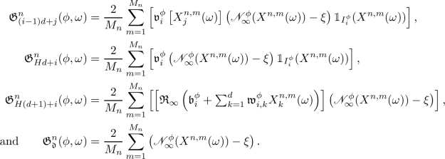
let $(M_n)_{n \in {\mathbb {N}}_0} \subseteq {\mathbb {N}}$, let ${\mathfrak {L}}^n_r :{\mathbb {R}}^{{\mathfrak {d}}} \times \Omega \rightarrow {\mathbb {R}}$, $n \in {\mathbb {N}}_0$, $r \in {\mathbb {N}}\cup \{ \infty \}$, satisfy for all $n \in {\mathbb {N}}_0$, $r \in {\mathbb {N}}\cup \{ \infty \}$, $\phi \in {\mathbb {R}}^{{\mathfrak {d}}}$, $\omega \in \Omega$ that , let ${\mathfrak {G}}^n = ({\mathfrak {G}}^n_1, \ldots , {\mathfrak {G}}^n_{{\mathfrak {d}}}) :{\mathbb {R}}^{{\mathfrak {d}}} \times \Omega \rightarrow {\mathbb {R}}^{{\mathfrak {d}}}$, $n \in {\mathbb {N}}_0$, satisfy for all $n \in {\mathbb {N}}_0$, $\phi \in {\mathbb {R}}^{\mathfrak {d}}$, that ${\mathfrak {G}}^n ( \phi , \omega ) = \lim _{r \rightarrow \infty } (\nabla _\phi {\mathfrak {L}}^n_r ) ( \phi , \omega )$, let $\Theta = (\Theta _n)_{n \in {\mathbb {N}}_0} :{\mathbb {N}}_0 \times \Omega \rightarrow {\mathbb {R}}^{ {\mathfrak {d}}}$ be a stochastic process, let $(\gamma _n)_{n \in {\mathbb {N}}_0} \subseteq [0, \infty )$, assume that $\Theta _0$ and $( X^{n,m} )_{(n,m) \in ( {\mathbb {N}}_0 ) ^2}$ are independent, and assume for all $n \in {\mathbb {N}}_0$, $\omega \in \Omega$ that $\Theta _{n+1} ( \omega ) = \Theta _n (\omega ) - \gamma _n {\mathfrak {G}}^{n} ( \Theta _n (\omega ), \omega )$.

3.2 Properties of the approximating empirical risk functions and their gradients

Proposition 3.2

Assume Setting 3.1 and let $n \in {\mathbb {N}}_0$, $\phi \in {\mathbb {R}}^{\mathfrak {d}}$, $\omega \in \Omega$. Then

• (i) it holds for all $r \in {\mathbb {N}}$, $i \in \{1, 2, \ldots , H\}$, $j \in \{1, 2, \ldots , d \}$ that

  

  (72)

• (ii) it holds that $\limsup _{r \rightarrow \infty } \Vert (\nabla {\mathfrak {L}}^n_r )(\phi , \omega ) - {\mathfrak {G}}^n ( \phi , \omega )\Vert = 0$, and

• (iii) it holds for all $i \in \{1, 2, \ldots , H\}$, $j \in \{1, 2, \ldots , d \}$ that

  

  (73)

Proof of Proposition 3.2

Observe that the assumption that for all $r \in {\mathbb {N}}$ it holds that ${\mathfrak {R}}_r \in C^1( {\mathbb {R}}, {\mathbb {R}})$ and the chain rule prove item (i). Next note that item (i) and the assumption that for all $x \in {\mathbb {R}}$ we have that $\limsup _{r \rightarrow \infty } \left( | {\mathfrak {R}}_r ( x ) - {\mathfrak {R}}_\infty ( x ) | + | ({\mathfrak {R}}_r)' ( x ) - \mathbb {1}_{\smash {(0, \infty )}} ( x ) |\right) = 0$ establish items (ii) and (iii). The proof of Proposition 3.2 is thus complete. $\square$

3.3 Properties of the expectations of the empirical risk functions

Proposition 3.3

Assume Setting 3.1. Then it holds for all $n \in {\mathbb {N}}_0$, $\phi \in {\mathbb {R}}^{{\mathfrak {d}}}$ that ${\mathbb {E}}[ {\mathfrak {L}}^n_\infty ( \phi ) ] = {\mathcal {L}}( \phi )$.

Proof of Proposition 3.3

Observe that the assumption that $X^{n,m} :\Omega \rightarrow [a,b]^d$, $n,m \in {\mathbb {N}}_0$, are i.i.d. random variables ensures that for all $n \in {\mathbb {N}}_0$, $\phi \in {\mathbb {R}}^{{\mathfrak {d}}}$ it holds that

(74)

The proof of Proposition 3.3 is thus complete. $\square$

Lemma 3.4

Assume Setting 3.1 and let ${\mathbb {F}}_n \subseteq {\mathcal {F}}$, $n \in {\mathbb {N}}_0$, satisfy for all $n \in {\mathbb {N}}$ that ${\mathbb {F}}_0 = \sigma ( \Theta _0)$ and ${\mathbb {F}}_n = \sigma \left( \Theta _0 , \left( X^{{\mathfrak {n}}, {\mathfrak {m}}}\right) _{({\mathfrak {n}}, {\mathfrak {m}}) \in ({\mathbb {N}}\cap [0,n) ) \times {\mathbb {N}}_0 } \right)$. Then

• (i) it holds for all $n \in {\mathbb {N}}_0$ that ${\mathbb {R}}^{{\mathfrak {d}}} \times \Omega \ni (\phi , \omega ) \mapsto {\mathfrak {G}}^n ( \phi , \omega ) \in {\mathbb {R}}^{\mathfrak {d}}$ is $({\mathcal {B}}({\mathbb {R}}^{\mathfrak {d}}) \otimes {\mathbb {F}}_{n+1} )/{\mathcal {B}}({\mathbb {R}}^{\mathfrak {d}})$-measurable,

• (ii) it holds for all $n \in {\mathbb {N}}_0$ that $\Theta _n$ is ${\mathbb {F}}_n/{\mathcal {B}}({\mathbb {R}}^{\mathfrak {d}})$-measurable, and

• (iii) it holds for all $m, n \in {\mathbb {N}}_0$ that $\sigma ( X^{n , m} )$ and ${\mathbb {F}}_n$ are independent.

Proof of Lemma 3.4

Note that Lemma 2.4 and (72) prove that for all $n \in {\mathbb {N}}_0$, $r \in {\mathbb {N}}$, $\omega \in \Omega$ it holds that ${\mathbb {R}}^{\mathfrak {d}}\ni \phi \mapsto (\nabla _\phi {\mathfrak {L}}_r^n ) ( \phi , \omega ) \in {\mathbb {R}}^{\mathfrak {d}}$ is continuous. Furthermore, observe that (72) and the fact that for all $n, m \in {\mathbb {N}}_0$ it holds that $X^{n,m}$ is ${\mathbb {F}}_{n+1}/{\mathcal {B}}( [a,b]^d)$-measurable assure that for all $n \in {\mathbb {N}}_0$, $r \in {\mathbb {N}}$, $\phi \in {\mathbb {R}}^{\mathfrak {d}}$ it holds that $\Omega \ni \omega \mapsto (\nabla _\phi {\mathfrak {L}}_r^n ) ( \phi , \omega ) \in {\mathbb {R}}^{\mathfrak {d}}$ is ${\mathbb {F}}_{n+1}/{\mathcal {B}}({\mathbb {R}}^{\mathfrak {d}})$-measurable. This and, e.g., [5, Lemma 2.4] show that for all $n \in {\mathbb {N}}_0$, $r \in {\mathbb {N}}$ it holds that ${\mathbb {R}}^{{\mathfrak {d}}} \times \Omega \ni (\phi , \omega ) \mapsto ( \nabla _\phi {\mathfrak {L}}_r^n ) ( \phi , \omega ) \in {\mathbb {R}}^{\mathfrak {d}}$ is $({\mathcal {B}}({\mathbb {R}}^{\mathfrak {d}}) \otimes {\mathbb {F}}_{n+1} )/{\mathcal {B}}({\mathbb {R}}^{\mathfrak {d}})$-measurable. Combining this with item (ii) in Proposition 3.2 demonstrates that for all $n \in {\mathbb {N}}_0$ it holds that

$$\begin{aligned} {\mathbb {R}}^{{\mathfrak {d}}} \times \Omega \ni (\phi , \omega ) \mapsto {\mathfrak {G}}^n ( \phi , \omega ) \in {\mathbb {R}}^{\mathfrak {d}}\end{aligned}$$

(75)

is $({\mathcal {B}}({\mathbb {R}}^{\mathfrak {d}}) \otimes {\mathbb {F}}_{n+1} )/{\mathcal {B}}({\mathbb {R}}^{\mathfrak {d}})$-measurable. This establishes item (i). In the next step we prove item (ii) by induction on $n \in {\mathbb {N}}_0$. Note that the fact that ${\mathbb {F}}_0 = \sigma ( \Theta _0)$ ensures that $\Theta _0$ is ${\mathbb {F}}_0/{\mathcal {B}}({\mathbb {R}}^{\mathfrak {d}})$-measurable. For the induction step let $n \in {\mathbb {N}}_0$ satisfy that $\Theta _n$ is ${\mathbb {F}}_n/{\mathcal {B}}( {\mathbb {R}}^{\mathfrak {d}})$-measurable. Observe that item (i) and the fact that ${\mathbb {F}}_n \subseteq {\mathbb {F}}_{n+1}$ ensure that ${\mathfrak {G}}^n ( \Theta _n)$ is ${\mathbb {F}}_{n+1}/{\mathcal {B}}({\mathbb {R}}^{\mathfrak {d}})$-measurable. Combining this, the fact that ${\mathbb {F}}_n \subseteq {\mathbb {F}}_{n+1}$, and the assumption that $\Theta _{n+1} = \Theta _n - \gamma _n {\mathfrak {G}}^{n} ( \Theta _n)$ demonstrates that $\Theta _{n+1}$ is ${\mathbb {F}}_{n+1}/{\mathcal {B}}({\mathbb {R}}^{\mathfrak {d}})$-measurable. Induction thus establishes item (ii). Next note that the assumption that $X^{n,m}$, $n, m \in {\mathbb {N}}_0$, are independent and the assumption that $\Theta _0$ and $( X^{n,m} )_{(n,m) \in ( {\mathbb {N}}_0 ) ^2}$ are independent establish item (iii). The proof of Lemma 3.4 is thus complete. $\square$

Corollary 3.5

Assume Setting 3.1. Then it holds for all $n \in {\mathbb {N}}_0$ that ${\mathbb {E}}[ {\mathfrak {L}}_\infty ^n ( \Theta _n ) ] = {\mathbb {E}}[ {\mathcal {L}}( \Theta _n ) ]$.

Proof of Corollary 3.5

Throughout this proof let ${\mathbb {F}}_n \subseteq {\mathcal {F}}$, $n \in {\mathbb {N}}_0$, satisfy for all $n \in {\mathbb {N}}$ that ${\mathbb {F}}_0 = \sigma ( \Theta _0)$ and ${\mathbb {F}}_n = \sigma \left( \Theta _0 , \left( X^{{\mathfrak {n}}, {\mathfrak {m}}}\right) _{({\mathfrak {n}}, {\mathfrak {m}}) \in ({\mathbb {N}}\cap [0,n) ) \times {\mathbb {N}}_0 } \right)$ and let ${\textbf{L}}^n :([a,b]^d)^{ M_n} \times {\mathbb {R}}^{ {\mathfrak {d}}} \rightarrow [0, \infty )$, $n \in {\mathbb {N}}_0$, satisfy for all $n \in {\mathbb {N}}_0$, $x_1, x_2, \ldots , x_{M_n} \in [a,b]^{d }$, $\phi \in {\mathbb {R}}^{ {\mathfrak {d}}}$ that

(76)

Observe that (76) implies that for all $n \in {\mathbb {N}}_0$, $\phi \in {\mathbb {R}}^{\mathfrak {d}}$, $\omega \in \Omega$ it holds that

$$\begin{aligned} {\mathfrak {L}}^n _\infty ( \phi , \omega ) = {\textbf{L}}^n ( X^{n, 1} ( \omega ), \ldots , X^{n, M_n}(\omega ) , \phi ). \end{aligned}$$

(77)

Hence, we obtain that for all $n \in {\mathbb {N}}_0$ it holds that

$$\begin{aligned} {\mathfrak {L}}_\infty ^n ( \Theta _n ) = {\textbf{L}}^n ( X^{n,1}, \ldots , X^{n , M_n}, \Theta _n ). \end{aligned}$$

(78)

Furthermore, note that (77) and Proposition 3.3 imply that for all $n \in {\mathbb {N}}_0$, $\phi \in {\mathbb {R}}^{{\mathfrak {d}}}$ we have that ${\mathbb {E}}[ {\textbf{L}}^n ( (X^{n, 1}, \ldots , X^{n, M_n}) , \phi ) ] = {\mathcal {L}}( \phi )$. This, Lemma 3.4, (78), and, e.g., [24, Lemma 2.8] (applied with $(\Omega , {\mathcal {F}}, {\mathbb {P}}) \curvearrowleft (\Omega , {\mathcal {F}}, {\mathbb {P}})$, ${\mathcal {G}}\curvearrowleft {\mathbb {F}}_n$, $({\mathbb {X}}, {\mathcal {X}}) \curvearrowleft (([a , b]^{d}) ^{ M_n} , {\mathcal {B}}(([a , b]^{d}) ^{ M_n}) )$, $({\mathbb {Y}}, {\mathcal {Y}}) \curvearrowleft ( {\mathbb {R}}^{{\mathfrak {d}}}, {\mathcal {B}}( {\mathbb {R}}^{\mathfrak {d}}) )$, $X \curvearrowleft (\Omega \ni \omega \mapsto ( X^{n, 1} (\omega ), \ldots , X^{n, M_n} ( \omega ) ) \in ([a , b]^{d}) ^{ M_n} )$, $Y \curvearrowleft (\Omega \ni \omega \mapsto \Theta _n ( \omega ) \in {\mathbb {R}}^{\mathfrak {d}})$ in the notation of [24, Lemma 2.8]) demonstrate that for all $n \in {\mathbb {N}}_0$ it holds that ${\mathbb {E}}[ {\mathfrak {L}}_\infty ^n ( \Theta _n ) ] = {\mathbb {E}}[ {\textbf{L}}^n ( X^{n, 1}, \ldots , X^{n, M_n} , \Theta _n) ] = {\mathbb {E}}[ {\mathcal {L}}( \Theta _n ) ]$. The proof of Corollary 3.5 is thus complete. $\square$

3.4 Upper estimates for generalized gradients of the empirical risk functions

Lemma 3.6

Assume Setting 3.1 and let $n \in {\mathbb {N}}_0$, $\phi \in {\mathbb {R}}^{\mathfrak {d}}$, $\omega \in \Omega$. Then $\Vert {\mathfrak {G}}^n ( \phi , \omega ) \Vert ^2 \le 4( {\textbf{a}}^2 (d+1) \Vert \phi \Vert ^2 + 1 ) {\mathfrak {L}}_\infty ^n ( \phi , \omega )$.

Proof of Lemma 3.6

Observe that Jensen’s inequality implies that

(79)

This and (73) ensure that for all $i \in \{1, 2, \ldots , H\}$, $j \in \{1,2, \ldots , d \}$ we have that

(80)

In addition, note that (73) and (79) assure that for all $i \in \{1,2, \ldots , H\}$ it holds that

(81)

Furthermore, observe that for all $x = (x_1, \ldots , x_d) \in [a,b]^d$, $i \in \{1,2, \ldots , H\}$ it holds that $| {\mathfrak {R}}_\infty \left( {\mathfrak {b}}^{\phi }_i + \textstyle \sum _{j = 1}^d {\mathfrak {w}}^{\phi }_{i,j} x_j \right) | ^2 \le \left( | {\mathfrak {b}}^{\phi }_i | + {\textbf{a}}\textstyle \sum _{j = 1}^d |{\mathfrak {w}}^{\phi }_{i,j} | \right) ^2 \le {\textbf{a}}^2 (d+1) \left( | {\mathfrak {b}}^{\phi }_i |^2 + \textstyle \sum _{j = 1}^d |{\mathfrak {w}}^{\phi }_{i,j} |^2 \right)$. Combining this, the fact that for all $m,n \in {\mathbb {N}}_0$, $\omega \in \Omega$ it holds that $X^{n,m} ( \omega ) \in [a,b]^d$, (73), and Jensen’s inequality demonstrates that for all $i \in \{1,2, \ldots , H\}$ it holds that

(82)

Moreover, note that (73) and (79) show that

(83)

Combining (80)–(83) yields

$$\begin{aligned} \begin{aligned}&\Vert {\mathfrak {G}}^n ( \phi , \omega ) \Vert ^2 \\&\quad \le 4 \left[ \textstyle \sum _{i = 1}^H\left( {\textbf{a}}^2 \left[ \sum _{j = 1}^d |{\mathfrak {v}}^{\phi }_i| ^2 \right] + |{\mathfrak {v}}^{\phi }_i| ^2 + {\textbf{a}}^2 (d+1) \left[ |{\mathfrak {b}}^{\phi }_i| ^2 + \textstyle \sum _{j = 1}^d |{\mathfrak {w}}^{\phi }_{i,j}| ^2 \right] \right) \right] {\mathfrak {L}}^n_\infty ( \phi , \omega ) + 4 {\mathfrak {L}}^n_\infty ( \phi , \omega ) \\&\quad \le 4 {\textbf{a}}^2 \left[ \textstyle \sum _{i=1}^H\left( (d+1) |{\mathfrak {v}}^{\phi }_i|^2 + (d+1) \left[ |{\mathfrak {b}}^{\phi }_i|^2 + \textstyle \sum _{j = 1}^d |{\mathfrak {w}}^{\phi }_{i,j}| ^2\right] \right) \right] {\mathfrak {L}}^n_\infty ( \phi , \omega ) + 4 {\mathfrak {L}}^n_\infty ( \phi , \omega )\\&\quad = 4({\textbf{a}}^2(d+1) \Vert \phi \Vert ^2 + 1) {\mathfrak {L}}^n_\infty ( \phi , \omega ). \end{aligned} \end{aligned}$$

(84)

The proof of Lemma 3.6 is thus complete. $\square$

Lemma 3.7

Assume Setting 3.1 and let $K \subseteq {\mathbb {R}}^{\mathfrak {d}}$ be compact. Then

$$\begin{aligned} \sup \nolimits _{n \in {\mathbb {N}}_0} \sup \nolimits _{\phi \in K } \sup \nolimits _{\omega \in \Omega } \Vert {\mathfrak {G}}^n ( \phi , \omega ) \Vert < \infty . \end{aligned}$$

(85)

Proof of Lemma 3.7

Observe that Lemma 2.4 proves that there exists ${\mathfrak {C}}\in {\mathbb {R}}$ which satisfies for all $\phi \in K$ that . The fact that for all $n , m\in {\mathbb {N}}_0$, $\omega \in \Omega$ it holds that $X^{n , m } (\omega ) \in [a,b]^d$ hence establishes that for all $n \in {\mathbb {N}}_0$, $\phi \in K$, $\omega \in \Omega$ we have that

(86)

Combining this and Lemma 3.6 completes the proof of Lemma 3.7. $\square$

3.5 Lyapunov type estimates for SGD processes

Lemma 3.8

Assume Setting 3.1 and let $n \in {\mathbb {N}}_0$, $\phi \in {\mathbb {R}}^{\mathfrak {d}}$, $\omega \in \Omega$. Then $\langle \nabla V ( \phi ) , {\mathfrak {G}}^n ( \phi , \omega ) \rangle = 8 {\mathfrak {L}}_\infty ^n ( \phi , \omega )$.

Proof of Lemma 3.8

Note that the fact that $V(\phi ) = \Vert \phi \Vert ^2 + |{\mathfrak {c}}^{\phi } - 2 \xi |^2$ ensures that

$$\begin{aligned}&(\nabla V) ( \phi ) \nonumber \\&\quad = 2 \left( {\mathfrak {w}}^{\phi }_{1,1}, \ldots , {\mathfrak {w}}^{\phi }_{1 , d}, {\mathfrak {w}}^{\phi }_{2 , 1}, \ldots , {\mathfrak {w}}^{\phi }_{2 , d}, \ldots , {\mathfrak {w}}^{\phi }_{H, 1}, \ldots , {\mathfrak {w}}^{\phi }_{H, d }, {\mathfrak {b}}^{\phi }_1, \ldots , {\mathfrak {b}}^{\phi }_{H}, {\mathfrak {v}}^{\phi }_1, \ldots , {\mathfrak {v}}^{\phi }_{H}, 2 ( {\mathfrak {c}}^{\phi } - \xi ) \right) . \end{aligned}$$

(87)

This and (73) imply that

(88)

Hence, we obtain that

(89)

The proof of Lemma 3.8 is thus complete. $\square$

Lemma 3.9

Assume Setting 3.1 and let $n \in {\mathbb {N}}_0$, $\theta \in {\mathbb {R}}^{\mathfrak {d}}$, $\omega \in \Omega$. Then

$$\begin{aligned} \begin{aligned} V ( \theta - \gamma _n {\mathfrak {G}}^n ( \theta , \omega ) ) - V ( \theta )&= (\gamma _n)^2 \Vert {\mathfrak {G}}^n ( \theta , \omega ) \Vert ^2 + (\gamma _n) ^2 |{\mathfrak {G}}^n_{\mathfrak {d}}( \theta , \omega ) | ^2 - 8 \gamma _n {\mathfrak {L}}^n_\infty ( \theta , \omega ) \\&\le 2 (\gamma _n)^2 \Vert {\mathfrak {G}}^n ( \theta , \omega ) \Vert ^2 - 8 \gamma _n {\mathfrak {L}}^n_\infty ( \theta , \omega ). \end{aligned} \end{aligned}$$

(90)

Proof of Lemma 3.9

Throughout this proof let ${\textbf{e}}\in {\mathbb {R}}^{\mathfrak {d}}$ satisfy ${\textbf{e}}= ( 0 , 0 , \ldots , 0 , 1)$ and let $g :{\mathbb {R}}\rightarrow {\mathbb {R}}$ satisfy for all $t \in {\mathbb {R}}$ that

$$\begin{aligned} g ( t ) = V ( \theta - t {\mathfrak {G}}^n ( \theta , \omega ) ). \end{aligned}$$

(91)

Observe that (91) and the fundamental theorem of calculus prove that

$$\begin{aligned} \begin{aligned} V ( \theta - \gamma _n {\mathfrak {G}}^n ( \theta , \omega ) )&= g ( \gamma _n ) = g ( 0 ) + \int \limits _0^{\gamma _n} g'(t) \, \textrm{d}t \\&= g ( 0 ) + \int \limits _0^{\gamma _n} \langle (\nabla V) ( \theta - t {\mathfrak {G}}^n ( \theta , \omega ) ) , ( - {\mathfrak {G}}( \theta , \omega ) ) \rangle \, \textrm{d}t \\&= V ( \theta ) - \int \limits _0^{\gamma _n} \langle ( \nabla V ) ( \theta - t {\mathfrak {G}}^n ( \theta , \omega ) ) , {\mathfrak {G}}( \theta , \omega ) \rangle \, \textrm{d}t. \end{aligned} \end{aligned}$$

(92)

Lemma 3.8 hence demonstrates that

$$\begin{aligned} \begin{aligned}&V ( \theta - \gamma _n {\mathfrak {G}}^n ( \theta , \omega ) ) \\&\quad = V ( \theta ) - \int \limits _0^{\gamma _n} \langle ( \nabla V ) ( \theta ) , {\mathfrak {G}}^n ( \theta , \omega ) \rangle \, \textrm{d}t \\&\qquad + \int \limits _0^{\gamma _n} \langle ( \nabla V ) ( \theta ) - ( \nabla V ) ( \theta - t {\mathfrak {G}}^n ( \theta , \omega ) ) , {\mathfrak {G}}^n ( \theta , \omega ) \rangle \, \textrm{d}t \\&\quad = V ( \theta ) - 8 \gamma _n {\mathfrak {L}}^n_\infty ( \theta ,\omega ) + \int \limits _0^{\gamma _n} \langle ( \nabla V ) ( \theta ) - ( \nabla V ) ( \theta - t {\mathfrak {G}}^n ( \theta , \omega ) ) , {\mathfrak {G}}^n ( \theta , \omega ) \rangle \, \textrm{d}t. \end{aligned} \end{aligned}$$

(93)

Proposition 2.8 therefore proves that

$$\begin{aligned} \begin{aligned} V ( \theta - \gamma _n {\mathfrak {G}}^n ( \theta , \omega ) )&= V ( \theta ) - 8 \gamma _n {\mathfrak {L}}^n_\infty ( \theta , \omega ) + \int \limits _0^{\gamma _n} \langle 2 t {\mathfrak {G}}^n ( \theta , \omega ) + 2 {\mathfrak {c}}^{t {\mathfrak {G}}^n ( \theta , \omega )} {\textbf{e}}, {\mathfrak {G}}^n ( \theta , \omega ) \rangle \, \textrm{d}t \\&= V ( \theta ) - 8 \gamma _n {\mathfrak {L}}^n_\infty ( \theta , \omega ) + 2 \Vert {\mathfrak {G}}^n ( \theta , \omega ) \Vert ^2 \left[ \int \limits _0^{\gamma _n} t \, \textrm{d}t \right] \\&\quad + 2 \left[ \int \limits _0^{\gamma _n} \left( {\mathfrak {c}}^{t {\mathfrak {G}}^n ( \theta , \omega )} \langle {\textbf{e}}, {\mathfrak {G}}^n ( \theta , \omega ) \rangle \right) \, \textrm{d}t \right] . \end{aligned} \end{aligned}$$

(94)

Hence, we obtain that

$$\begin{aligned} \begin{aligned}&V ( \theta - \gamma _n {\mathfrak {G}}^n ( \theta , \omega ) ) \\&\quad = V ( \theta ) - 8 \gamma _n {\mathfrak {L}}^n_\infty ( \theta , \omega ) + (\gamma _n) ^2 \Vert {\mathfrak {G}}^n ( \theta , \omega ) \Vert ^2 + 2 |\langle {\textbf{e}}, {\mathfrak {G}}^n ( \theta , \omega ) \rangle |^2 \left[ \int \limits _0^{\gamma _n} t \, \textrm{d}t \right] \\&\quad = V ( \theta ) - 8 \gamma _n {\mathfrak {L}}^n_\infty ( \theta , \omega ) + (\gamma _n)^2 \Vert {\mathfrak {G}}^n ( \theta , \omega ) \Vert ^2 + (\gamma _n) ^2 |\langle {\textbf{e}}, {\mathfrak {G}}^n ( \theta , \omega ) \rangle |^2 \\&\quad = V ( \theta ) - 8 \gamma _n {\mathfrak {L}}^n_\infty ( \theta , \omega ) + (\gamma _n) ^2 \Vert {\mathfrak {G}}^n ( \theta , \omega ) \Vert ^2 + (\gamma _n) ^2 |{\mathfrak {G}}^n_{\mathfrak {d}}( \theta , \omega ) | ^2. \end{aligned} \end{aligned}$$

(95)

The proof of Lemma 3.9 is thus complete. $\square$

Lemma 3.10

Assume Setting 3.1. Then it holds for all $n \in {\mathbb {N}}_0$ that

$$\begin{aligned} V(\Theta _{n+1}) - V ( \Theta _n) \le 8 \left( (\gamma _n) ^2 \left[ {\textbf{a}}^2 (d+1) V(\Theta _n) + 1 \right] - \gamma _n \right) {\mathfrak {L}}^n_\infty ( \Theta _ n) . \end{aligned}$$

(96)

Proof of Lemma 3.10

Note that Lemmas 2.7 and 3.6 prove that for all $n \in {\mathbb {N}}_0$ it holds that

$$\begin{aligned} \Vert {\mathfrak {G}}^n ( \Theta _n ) \Vert ^2 \le 4 \left[ {\textbf{a}}^2 (d+1) \Vert \Theta _n \Vert ^2 + 1 \right] {\mathfrak {L}}_\infty ^n ( \Theta _n ) \le 4 \left[ {\textbf{a}}^2 (d+1) V ( \Theta _n ) + 1 \right] {\mathfrak {L}}_\infty ^n ( \Theta _n ). \end{aligned}$$

(97)

Lemma 3.9 hence demonstrates that for all $n \in {\mathbb {N}}_0$ it holds that

$$\begin{aligned} \begin{aligned} V ( \Theta _{n+1} ) - V ( \Theta _n )&\le 2 ( \gamma _n)^2 \Vert {\mathfrak {G}}^n ( \Theta _n ) \Vert ^2 - 8 \gamma _n {\mathfrak {L}}_\infty ^n ( \Theta _n ) \\&\le 8 (\gamma _n)^2 \left[ {\textbf{a}}^2 (d+1) V ( \Theta _n ) + 1 \right] {\mathfrak {L}}_\infty ^n ( \Theta _n ) - 8 \gamma _n {\mathfrak {L}}_\infty ^n ( \Theta _n ) \\&= 8 \left( (\gamma _n) ^2 \left[ {\textbf{a}}^2 (d+1) V(\Theta _n) + 1 \right] - \gamma _n \right) {\mathfrak {L}}^n_\infty ( \Theta _ n) . \end{aligned} \end{aligned}$$

(98)

The proof of Lemma 3.10 is thus complete. $\square$

Corollary 3.11

Assume Setting 3.1 and assume ${\mathbb {P}}\left( \sup _{n \in {\mathbb {N}}_0} \gamma _n \le \left[ {\textbf{a}}^2(d+1)V(\Theta _0) + 1\right] ^{-1} \right) = 1$. Then it holds for all $n \in {\mathbb {N}}_0$ that

$$\begin{aligned} {\mathbb {P}}\left( V(\Theta _{n+1} ) - V(\Theta _n) \le - 8 \gamma _n \left( 1 - \left[ \sup \nolimits _{m \in {\mathbb {N}}_0} \gamma _m \right] \left[ {\textbf{a}}^2(d+1)V(\Theta _0) + 1\right] \right) {\mathfrak {L}}_\infty ^n ( \Theta _n ) \le 0 \right) = 1. \end{aligned}$$

(99)

Proof of Corollary 3.11

Throughout this proof let ${\mathfrak {g}}\in {\mathbb {R}}$ satisfy ${\mathfrak {g}}= \sup _{n \in {\mathbb {N}}_0} \gamma _n$. We now prove (99) by induction on $n \in {\mathbb {N}}_0$. Observe that Lemma 3.10 and the fact that $\gamma _0 \le {\mathfrak {g}}$ imply that it holds ${\mathbb {P}}$-a.s. that

$$\begin{aligned} \begin{aligned} V(\Theta _1) - V(\Theta _0)&\le 8 \left( ( \gamma _0 )^2 \left[ {\textbf{a}}^2 (d+1) V(\Theta _0) + 1 \right] - \gamma _0 \right) {\mathfrak {L}}^0_\infty ( \Theta _ 0) \\&\le 8 \left( \gamma _0 {\mathfrak {g}}\left[ {\textbf{a}}^2 (d+1) V(\Theta _0) + 1 \right] - \gamma _0 \right) {\mathfrak {L}}^0_\infty ( \Theta _ 0) \\&= - 8 \gamma _0 \left( 1 - {\mathfrak {g}}\left[ {\textbf{a}}^2(d+1)V(\Theta _0) + 1\right] \right) {\mathfrak {L}}^0_\infty ( \Theta _ 0). \end{aligned} \end{aligned}$$

(100)

This establishes (99) in the base case $n=0$. For the induction step let $n \in {\mathbb {N}}$ satisfy that for all $m \in \{0, 1, \ldots , n-1\}$ it holds ${\mathbb {P}}$-a.s. that

$$\begin{aligned} V( \Theta _{m + 1}) - V ( \Theta _{m} ) \le - 8 \gamma _m \left( 1 - {\mathfrak {g}}\left[ {\textbf{a}}^2 (d+1) V(\Theta _0) + 1\right] \right) {\mathfrak {L}}_\infty ^m ( \Theta _m ) \le 0. \end{aligned}$$

(101)

Note that (101) shows that it holds ${\mathbb {P}}$-a.s. that $V(\Theta _n) \le V(\Theta _{n-1}) \le \cdots \le V(\Theta _0)$. The fact that $\gamma _n \le {\mathfrak {g}}$ and Lemma 3.10 hence demonstrate that it holds ${\mathbb {P}}$-a.s. that

$$\begin{aligned} \begin{aligned} V(\Theta _{n+1}) - V(\Theta _n)&\le 8 \left( ( \gamma _n )^2 \left[ {\textbf{a}}^2 (d+1) V(\Theta _n) + 1 \right] - \gamma _n \right) {\mathfrak {L}}_\infty ^n ( \Theta _ n) \\&\le 8 \left( \gamma _n {\mathfrak {g}}\left[ {\textbf{a}}^2 (d+1) V(\Theta _n) + 1 \right] - \gamma _n \right) {\mathfrak {L}}_\infty ^n ( \Theta _ n) \\&= - 8 \gamma _n \left( 1 - {\mathfrak {g}}\left[ {\textbf{a}}^2(d+1)V(\Theta _0) + 1\right] \right) {\mathfrak {L}}_\infty ^n ( \Theta _n ) \le 0. \end{aligned} \end{aligned}$$

(102)

Induction therefore establishes (99). The proof of Corollary 3.11 is thus complete. $\square$

3.6 Convergence analysis for SGD processes in the training of ANNs

Theorem 3.12

Assume Setting 3.1, let $\delta \in (0, 1)$, assume $\sum _{n=0}^\infty \gamma _n = \infty$, and assume for all $n \in {\mathbb {N}}_0$ that ${\mathbb {P}}\left( \gamma _n \left[ {\textbf{a}}^2 (d+1) V ( \Theta _ 0 ) + 1\right] \le \delta \right) = 1$. Then

• (i) there exists ${\mathfrak {C}}\in {\mathbb {R}}$ such that ${\mathbb {P}}\left( \sup _{n \in {\mathbb {N}}_0} \Vert \Theta _n \Vert \le {\mathfrak {C}}\right) = 1$,

• (ii) it holds that ${\mathbb {P}}\left( \limsup _{n \rightarrow \infty } {\mathcal {L}}( \Theta _n ) = 0 \right) = 1$, and

• (iii) it holds that $\limsup _{n \rightarrow \infty } {\mathbb {E}}[ {\mathcal {L}}( \Theta _n ) ] = 0$.

Proof of Theorem 3.12

Throughout this proof let ${\mathfrak {g}}\in [0 , \infty ]$ satisfy ${\mathfrak {g}}= \sup _{n \in {\mathbb {N}}_0} \gamma _n$. Observe that the assumption that $\delta < 1$, the fact that ${\mathbb {P}}\left( {\mathfrak {g}}\left[ {\textbf{a}}^2 (d+1) V ( \Theta _ 0 ) + 1\right] \le \delta \right) = 1$, and the assumption that $\sum _{n=0}^\infty \gamma _n = \infty$ demonstrate that ${\mathfrak {g}}\in (0, \infty )$. This and the fact that ${\mathbb {P}}\left( {\mathfrak {g}}\left[ {\textbf{a}}^2 (d+1) V ( \Theta _ 0 ) + 1\right] \le \delta \right) = 1$ show that there exists ${\mathfrak {C}}\in [1 , \infty )$ which satisfies that

$$\begin{aligned} {\mathbb {P}}( V(\Theta _0 ) \le {\mathfrak {C}}) = 1. \end{aligned}$$

(103)

Note that (103) and Corollary 3.11 ensure that ${\mathbb {P}}\left( \sup _{ n \in {\mathbb {N}}_0 } V(\Theta _n) \le {\mathfrak {C}}\right) = 1$. Combining this and the fact that for all $\phi \in {\mathbb {R}}^{\mathfrak {d}}$ it holds that $\Vert \phi \Vert \le \left[ V ( \phi ) \right] ^{1/2}$ demonstrates that

$$\begin{aligned} {\mathbb {P}}\left( \sup \nolimits _{n \in {\mathbb {N}}_0} \Vert \Theta _n\Vert \le {\mathfrak {C}}\right) = 1. \end{aligned}$$

(104)

This establishes item (i). Next observe that Corollary 3.11 and the fact that ${\mathbb {P}}( {\mathfrak {g}}\left[ {\textbf{a}}^2 (d+1) V ( \Theta _ 0 ) + 1\right] \le \delta ) = 1$ prove that for all $n \in {\mathbb {N}}_0$ it holds ${\mathbb {P}}$-a.s. that

$$\begin{aligned} - \left( V(\Theta _{n} ) - V(\Theta _{n+1}) \right) \le - 8 \gamma _n \left( 1 - {\mathfrak {g}}\left[ {\textbf{a}}^2(d+1)V(\Theta _0) + 1\right] \right) {\mathfrak {L}}_\infty ^n ( \Theta _n ). \end{aligned}$$

(105)

This assures that for all $n \in {\mathbb {N}}_0$ it holds ${\mathbb {P}}$-a.s. that

$$\begin{aligned} \gamma _n {\mathfrak {L}}_\infty ^n ( \Theta _n ) \le \frac{ V ( \Theta _n ) - V ( \Theta _{n+1})}{ 8 ( 1 - {\mathfrak {g}}\left[ {\textbf{a}}^2 ( d+1) V ( \Theta _0 ) + 1 \right] ) }. \end{aligned}$$

(106)

The fact that ${\mathbb {P}}\left( {\mathfrak {g}}\left[ {\textbf{a}}^2 (d+1) V ( \Theta _ 0 ) + 1\right] \le \delta \right) = 1$ and (103) hence show that for all $N \in {\mathbb {N}}$ it holds ${\mathbb {P}}$-a.s. that

$$\begin{aligned} \begin{aligned} \sum _{n = 0}^{N - 1} \gamma _n {\mathfrak {L}}_\infty ^n ( \Theta _ n )&\le \frac{\textstyle \sum _{n=0}^{N-1} ( V ( \Theta _n ) - V ( \Theta _{n+1} ) )}{8 ( 1 - {\mathfrak {g}}\left[ {\textbf{a}}^2 ( d+1) V ( \Theta _0 ) + 1 \right] )} = \frac{ V ( \Theta _{0}) - V ( \Theta _N ) }{8 (1 - {\mathfrak {g}}\left[ {\textbf{a}}^2 (d+1) V ( \Theta _ 0 ) + 1\right] )} \\&\le \frac{V ( \Theta _0) }{8 (1-\delta ) } \le \frac{{\mathfrak {C}}}{8(1-\delta )} < \infty . \end{aligned} \end{aligned}$$

(107)

This implies that

$$\begin{aligned} \sum _{n=0}^\infty \gamma _n {\mathbb {E}}[ {\mathfrak {L}}_\infty ^n ( \Theta _n )] = \lim _{N \rightarrow \infty } \left[ \sum _{n=0}^{N-1} \gamma _n {\mathbb {E}}[ {\mathfrak {L}}_\infty ^n ( \Theta _n ) ] \right] \le \frac{{\mathfrak {C}}}{8(1-\delta )} < \infty . \end{aligned}$$

(108)

Furthermore, note that Corollary 3.5 shows for all $n \in {\mathbb {N}}_0$ that ${\mathbb {E}}[ {\mathfrak {L}}_\infty ^n ( \Theta _n )] = {\mathbb {E}}[ {\mathcal {L}}( \Theta _n )]$. Combining this with (108) proves that

$$\begin{aligned} \sum _{n=0}^\infty {\mathbb {E}}[\gamma _n {\mathcal {L}}( \Theta _n ) ] < \infty . \end{aligned}$$

(109)

The monotone convergence theorem and the fact that for all $n \in {\mathbb {N}}_0$ it holds that ${\mathcal {L}}( \Theta _n ) \ge 0$ hence demonstrate that

$$\begin{aligned} {\mathbb {E}}\left[ \sum _{n=0}^\infty \gamma _n {\mathcal {L}}( \Theta _n ) \right] = \sum _{n=0}^\infty {\mathbb {E}}[\gamma _n {\mathcal {L}}( \Theta _n ) ] < \infty . \end{aligned}$$

(110)

Hence, we obtain that ${\mathbb {P}}\left( \sum _{n=0}^\infty \gamma _n {\mathcal {L}}( \Theta _n ) < \infty \right) = 1$. Next let $A \subseteq \Omega$ satisfy

$$\begin{aligned} A = \left\{ \omega \in \Omega :\left[ \left( \textstyle \sum _{n=0}^\infty \gamma _n {\mathcal {L}}( \Theta _n (\omega ) ) < \infty \right) \wedge \left( \sup \nolimits _{n \in {\mathbb {N}}_0} \Vert \Theta _n ( \omega ) \Vert \le {\mathfrak {C}}\right) \right] \right\} . \end{aligned}$$

(111)

Observe that (104) and the fact that ${\mathbb {P}}( \textstyle \sum _{n=0}^\infty \gamma _n {\mathcal {L}}( \Theta _n) < \infty ) = 1$ prove that $A \in {\mathcal {F}}$ and ${\mathbb {P}}( A ) = 1$. In the following let $\omega \in A$ be arbitrary. Note that the assumption that $\sum _{n=0}^\infty \gamma _n = \infty$ and the fact that $\textstyle \sum _{n=0}^\infty \gamma _n {\mathcal {L}}( \Theta _n (\omega ) ) < \infty$ demonstrate that $\liminf _{n \rightarrow \infty } {\mathcal {L}}( \Theta _n ( \omega )) = 0$. We intend to prove by a contradiction that $\limsup _{n \rightarrow \infty } {\mathcal {L}}( \Theta _n ( \omega )) = 0$. In the following we thus assume that $\limsup _{n \rightarrow \infty } {\mathcal {L}}( \Theta _n ( \omega )) > 0$. This implies that there exists $\varepsilon \in (0 , \infty )$ which satisfies that

$$\begin{aligned} 0 = \liminf _{n \rightarrow \infty } {\mathcal {L}}( \Theta _n ( \omega ))< \varepsilon< 2 \varepsilon < \limsup _{n \rightarrow \infty } {\mathcal {L}}( \Theta _n ( \omega )). \end{aligned}$$

(112)

Hence, we obtain that there exist $(m_k, n_k) \in {\mathbb {N}}^2$, $k \in {\mathbb {N}}$, which satisfy for all $k \in {\mathbb {N}}$ that $m_k< n_k < m_{k+1}$, ${\mathcal {L}}( \Theta _{m_k} ( \omega ) ) > 2 \varepsilon$, and ${\mathcal {L}}( \Theta _{n_k} ( \omega ) ) < \varepsilon \le \min _{j \in {\mathbb {N}}\cap [m_k, n_k ) } {\mathcal {L}}( \Theta _j ( \omega ) )$. Observe that the fact that $\sum _{n=0}^\infty \gamma _n {\mathcal {L}}( \Theta _n (\omega ) ) < \infty$ and the fact that for all $k \in {\mathbb {N}}$, $j \in {\mathbb {N}}\cap [m_k, n_k )$ it holds that $1 \le \varepsilon ^{-1} {\mathcal {L}}( \Theta _j ( \omega ) )$ assure that

$$\begin{aligned} \sum _{k=1}^\infty \sum _{j=m_k}^{n_k - 1} \gamma _j \le \frac{1}{\varepsilon } \left[ \sum _{k=1}^\infty \sum _{j=m_k}^{n_k - 1} \left( \gamma _j {\mathcal {L}}( \Theta _j (\omega ) ) \right) \right] \le \frac{1}{\varepsilon } \left[ \sum _{j=0}^\infty \left( \gamma _j {\mathcal {L}}( \Theta _j ( \omega ) ) \right) \right] < \infty . \end{aligned}$$

(113)

Next note that the fact that $\sup \nolimits _{n \in {\mathbb {N}}_0} \Vert \Theta _n ( \omega ) \Vert \le {\mathfrak {C}}$ and Lemma 3.7 ensure that there exists ${\mathfrak {D}}\in {\mathbb {R}}$ which satisfies for all $n \in {\mathbb {N}}_0$ that $\Vert {\mathfrak {G}}^n ( \Theta _n (\omega ) , \omega ) \Vert \le {\mathfrak {D}}$. Combining this and (113) proves that

$$\begin{aligned} \begin{aligned} \sum _{k=1}^\infty \Vert \Theta _{n_k}(\omega ) - \Theta _{m_k}(\omega ) \Vert&\le \sum _{k=1}^\infty \sum _{j=m_k}^{n_k - 1} \Vert \Theta _{j+1}(\omega ) - \Theta _j (\omega ) \Vert = \sum _{k=1}^\infty \sum _{j=m_k}^{n_k - 1} \left( \gamma _j \Vert {\mathfrak {G}}^j ( \Theta _j (\omega ) , \omega ) \Vert \right) \\&\le {\mathfrak {D}}\left[ \sum _{k=1}^\infty \sum _{j=m_k}^{n_k - 1} \gamma _j \right] < \infty . \end{aligned} \end{aligned}$$

(114)

Moreover, observe that the fact that $\sup \nolimits _{n \in {\mathbb {N}}_0} \Vert \Theta _n ( \omega ) \Vert \le {\mathfrak {C}}$ and Lemma 2.4 show that there exists which satisfies for all $m, n \in {\mathbb {N}}_0$ that . This and (114) demonstrate that

(115)

Combining this and the fact that for all $k \in {\mathbb {N}}_0$ it holds that ${\mathcal {L}}( \Theta _{n_k} (\omega ) )< \varepsilon< 2 \varepsilon < {\mathcal {L}}( \Theta _{m_k} ( \omega ) )$ ensures that

$$\begin{aligned} 0 < \varepsilon \le \inf _{k \in {\mathbb {N}}} | {\mathcal {L}}( \Theta _{n_k} (\omega ) ) - {\mathcal {L}}( \Theta _{m_k} ( \omega ) ) | \le \limsup _{k \rightarrow \infty } | {\mathcal {L}}( \Theta _{n_k} ( \omega ) ) - {\mathcal {L}}( \Theta _{m_k} ( \omega ) ) | = 0. \end{aligned}$$

(116)

This contradiction proves that $\limsup _{n \rightarrow \infty } {\mathcal {L}}( \Theta _n ( \omega )) = 0$. This and the fact that ${\mathbb {P}}( A ) = 1$ establish item (ii). Next note that item (i) and the fact that ${\mathcal {L}}$ is continuous show that there exists which satisfies that . This, item (ii), and the dominated convergence theorem establish item (iii). The proof of Theorem 3.12 is thus complete. $\square$

Corollary 3.13

Assume Setting 3.1, let ${\textbf{A}}\in {\mathbb {R}}$ satisfy ${\textbf{A}}= \max \{ {\textbf{a}}, |\xi | \}$, assume $\sum _{n=0}^\infty \gamma _n = \infty$, and assume for all $n \in {\mathbb {N}}_0$ that ${\mathbb {P}}\left( 18 {\textbf{A}}^4 d \gamma _n \le ( \Vert \Theta _0\Vert + 1 )^{-2} \right) = 1$. Then

• (i) there exists ${\mathfrak {C}}\in {\mathbb {R}}$ such that ${\mathbb {P}}\left( \sup _{n \in {\mathbb {N}}_0} \Vert \Theta _n \Vert \le {\mathfrak {C}}\right) = 1$,

• (ii) it holds that ${\mathbb {P}}\left( \limsup _{n \rightarrow \infty } {\mathcal {L}}( \Theta _n ) = 0 \right) = 1$, and

• (iii) it holds that $\limsup _{n \rightarrow \infty } {\mathbb {E}}[ {\mathcal {L}}( \Theta _n ) ] = 0$.

Proof of Corollary 3.13

Observe that Lemma 2.7 proves that it holds ${\mathbb {P}}$-a.s. that

$$\begin{aligned} {\textbf{a}}^2 (d+1) V ( \Theta _ 0 ) + 1 \le 3 {\textbf{a}}^2 (d+1) \Vert \Theta _0\Vert ^2 + 8 \xi ^2 {\textbf{a}}^2 (d+1) + 1 . \end{aligned}$$

(117)

The fact that $\min \left\{ {\textbf{A}}, d \right\} \ge 1$ hence shows that it holds ${\mathbb {P}}$-a.s. that

$$\begin{aligned} {\textbf{a}}^2 (d+1) V ( \Theta _ 0 ) + 1\le 6 {\textbf{A}}^2 d \Vert \Theta _0\Vert ^2 + 16 {\textbf{A}}^4 d + 1 \le 17 {\textbf{A}}^4 d (\Vert \Theta _0\Vert ^2 + 1) \le 17 {\textbf{A}}^4 d (\Vert \Theta _0\Vert + 1)^2. \end{aligned}$$

(118)

This and the assumption that for all $n \in {\mathbb {N}}_0$ it holds that ${\mathbb {P}}\left( 18 {\textbf{A}}^4 d \gamma _n \le ( \Vert \Theta _0\Vert + 1 )^{-2} \right) = 1$ ensure that for all $n \in {\mathbb {N}}_0$ it holds ${\mathbb {P}}$-a.s. that

$$\begin{aligned} \gamma _n \left( {\textbf{a}}^2 (d+1) V ( \Theta _ 0 ) + 1\right) \le 17 {\textbf{A}}^4 d \gamma _n (\Vert \Theta _0\Vert + 1)^2 \le \tfrac{17}{18} < 1. \end{aligned}$$

(119)

Theorem 3.12 hence establishes items (i), (ii), and (iii). The proof of Corollary 3.13 is thus complete. $\square$

3.7 A Python code for generalized gradients of the loss functions

In this subsection we include a short illustrative example Python code for the computation of appropriate generalized gradients of the risk function. In the notation of Setting 3.1 we assume in the Python code in Listing 1 below that $d=1$, $H= 3$, ${\mathfrak {d}}= 10$, $\phi = (-1, 1, 2, 2, -2, 0, 1, -1, 2, 3) \in {\mathbb {R}}^{10}$, $\xi = 3$, $\omega \in \Omega$, and $X^{1,1}(\omega ) = 2$. Observe that in this situation it holds that ${\mathfrak {w}}^{\phi }_{1,1} X^{1,1} ( \omega ) + {\mathfrak {b}}^{\phi }_1 = {\mathfrak {w}}^{\phi }_{2,1} X^{1,1} ( \omega ) + {\mathfrak {b}}^{\phi }_2=0$. Listing 2 presents the output of a call of the Python code in Listing 1. Listing 2 illustrates that the computed generalized partial derivatives of the loss with respect to ${\mathfrak {w}}^{\phi }_{1,1}$, ${\mathfrak {w}}^{\phi }_{2,1}$, ${\mathfrak {b}}^{\phi }_1$, ${\mathfrak {b}}^{\phi }_2$, ${\mathfrak {v}}^{\phi }_1$, and ${\mathfrak {v}}^{\phi }_2$ vanish. Note that (73) and the fact that $\mathbb {1}_{\smash {I_1^\phi }} (X^{1,1}(\omega )) = \mathbb {1}_{\smash {I_2^\phi }} ( X^{1,1}(\omega ) ) = 0$ prove that the generalized partial derivatives of the loss with respect to ${\mathfrak {w}}^{\phi }_{1,1}$, ${\mathfrak {w}}^{\phi }_{2,1}$, ${\mathfrak {b}}^{\phi }_1$, ${\mathfrak {b}}^{\phi }_2$, ${\mathfrak {v}}^{\phi }_1$, and ${\mathfrak {v}}^{\phi }_2$ do vanish.

References

Akyildiz, Ö.D., Sabanis, S.: Nonasymptotic analysis of Stochastic Gradient Hamiltonian Monte Carlo under local conditions for nonconvex optimization (2021). arXiv:2002.05465
Allen-Zhu, Z., Li, Y., Liang, Y.: Learning and generalization in overparameterized neural networks, going beyond two layers. In Wallach, H., Larochelle, H., Beygelzimer, A., d’ Alché-Buc, F., Fox, E., Garnett, R. (eds.), Advances in Neural Information Processing Systems, Vol. 32, pp. 6158–6169. Curran Associates, Inc., (2019). https://proceedings.neurips.cc/paper/2019/file/62dad6e273d32235ae02b7d321578ee8-Paper.pdf
Allen-Zhu, Z., Li, Y., Song, Z.: A convergence theory for deep learning via over-parameterization. In: Chaudhuri, K., Salakhutdinov, R., (eds.) Proceedings of the 36th International Conference on Machine Learning, volume 97 of Proceedings of Machine Learning Research, pp. 242–252. PMLR, 09–15. http://proceedings.mlr.press/v97/allen-zhu19a.html (2019)
Bach, F., Moulines, E.: Non-strongly-convex smooth stochastic approximation with convergence rate \(O(1/n)\). In: Burges, C.J.C., Bottou, L., Welling, M., Ghahramani, Z., Weinberger, K.Q. (eds.) Advances in Neural Information Processing Systems, Vol. 26, pp. 773–781. Curran Associates, Inc. http://papers.nips.cc/paper/4900-non-strongly-convex-smooth-stochastic-approximation-with-convergence-rate-o1n.pdf (2013)
Beck, C., Becker, S., Grohs, P., Jaafari, N., Jentzen, A.: Solving stochastic differential equations and Kolmogorov equations by means of deep learning, 2018. Published in Journal of Scientific Computing. arXiv:1806.00421 (2021)
Beck, C., Jentzen, A., Kuckuck, B.:. Full error analysis for the training of deep neural networks. Infin. Dimens. Anal. Quantum Probab. Relat. Top. 25(2):Paper No. 2150020, 76 (2022). https://doi.org/10.1142/S021902572150020X.
Bertsekas, D.P., Tsitsiklis, J.N.: Gradient convergence in gradient methods with errors. SIAM J. Optim. 10(3), 627–642 (2000). https://doi.org/10.1137/S1052623497331063
Bottou, L., Curtis, F.E., Nocedal, J.: Optimization methods for large-scale machine learning. arXiv:1606.04838 (2018)
Cheridito, P., Jentzen, A., Riekert, A., Rossmannek, F.: A proof of convergence for gradient descent in the training of artificial neural networks for constant target functions. J. Complex. (2022). https://doi.org/10.1016/j.jco.2022.101646
Cheridito, P., Jentzen, A., Rossmannek, F.: Non-convergence of stochastic gradient descent in the training of deep neural networks. J. Complex. (2020). https://doi.org/10.1016/j.jco.2020.101540
Cheridito, P., Jentzen, A., Rossmannek, F.: Landscape analysis for shallow neural networks: complete classification of critical points for affine target functions. J. Nonlinear Sci. 32(5):Paper No. 64 (2022). https://doi.org/10.1007/s00332-022-09823-8
Chizat, L., Bach, F.: On the global convergence of gradient descent for over-parameterized models using optimal transport. In: Bengio, S., Wallach, H., Larochelle, H., Grauman, K., Cesa-Bianchi, N., Garnett, R. (eds.) Advances in Neural Information Processing Systems, Vol. 31, pp. 3036–3046. Curran Associates, Inc. https://proceedings.neurips.cc/paper/2018/file/a1afc58c6ca9540d057299ec3016d726-Paper.pdf (2018)
Dereich, S., Kassing, S.: Convergence of stochastic gradient descent schemes for Lojasiewicz-landscapes. arXiv:2102.09385 (2021)
Dereich, S., Müller-Gronbach, T.: General multilevel adaptations for stochastic approximation algorithms of Robbins–Monro and Polyak–Ruppert type. Numer. Math. 142(2), 279–328 (2019). https://doi.org/10.1007/s00211-019-01024-y
Du, S., Lee, J., Li, H., Wang, L., Zhai, X.: Gradient descent finds global minima of deep neural networks. In: Chaudhuri, K., Salakhutdinov, R. (eds.) Proceedings of the 36th International Conference on Machine Learning, Volume 97 of Proceedings of Machine Learning Research, pp. 1675–1685, Long Beach, California, USA, 6. PMLR. http://proceedings.mlr.press/v97/du19c.html (2019)
Du, S.S., Zhai, X., Poczós, B., Singh, A.: Gradient descent provably optimizes over-parameterized neural networks. arXiv:1810.02054 (2018)
E, W., Ma, C., Wu, L.: A comparative analysis of optimization and generalization properties of two-layer neural network and random feature models under gradient descent dynamics. Sci. China Math. 63(7), 1235–1258 (2020). https://doi.org/10.1007/s11425-019-1628-5
Fehrman, B., Gess, B., Jentzen, A.: Convergence rates for the stochastic gradient descent method for non-convex objective functions. J. Mach. Learn. Res. 21(136), 1–48 (2020)
Ge, R., Huang, F., Jin, C., Yuan, Y.: Escaping from saddle points—online stochastic gradient for tensor decomposition. In: Grónwald, P., Hazan, E., Kale, S. (eds.) Proceedings of the 28th Conference on Learning Theory, Volume 40 of Proceedings of Machine Learning Research, pp. 797–842, Paris, France, 03–06. PMLR (2015)
Goodfellow, I., Bengio, Y., Courville, A.: Deep learning. In: Adaptive Computation and Machine Learning. MIT Press, Cambridge (2016)
Hanin, B.: Which neural net architectures give rise to exploding and vanishing gradients? In: Bengio, S., Wallach, H., Larochelle, H., Grauman, K., Cesa-Bianchi, N., Garnett, R. (eds.) Advances in Neural Information Processing Systems, Vol. 31, pp. 582–591. Curran Associates, Inc. https://proceedings.neurips.cc/paper/2018/file/13f9896df61279c928f19721878fac41-Paper.pdf (2018)
Hanin, B., Rolnick, D.: How to start training: The effect of initialization and architecture. In: Bengio, S., Wallach, H., Larochelle, H., Grauman, K., Cesa-Bianchi, N., Garnett, R. (eds.) Advances in Neural Information Processing Systems, Volume 31, pp. 571–581. Curran Associates, Inc. https://proceedings.neurips.cc/paper/2018/file/d81f9c1be2e08964bf9f24b15f0e4900-Paper.pdf (2018)
Jentzen, A., Kröger, T.: Convergence rates for gradient descent in the training of overparameterized artificial neural networks with biases. arXiv:2102.11840 (2021)
Jentzen, A., Kuckuck, B., Neufeld, A., von Wurstemberger, P.: Strong error analysis for stochastic gradient descent optimization algorithms, 2018. Published in IMA J. Numer. Anal. arXiv:1801.09324 (2021)
Jentzen, A., von Wurstemberger, P.: Lower error bounds for the stochastic gradient descent optimization algorithm: sharp convergence rates for slowly and fast decaying learning rates. J. Complex. 57, 101438 (2020). https://doi.org/10.1016/j.jco.2019.101438
Jentzen, A., Welti, T.: Overall error analysis for the training of deep neural networks via stochastic gradient descent with random initialisation. arXiv:2003.01291v1 (2020)
Karimi, B., Miasojedow, B., Moulines, E., Wai, H.-T.: Non-asymptotic analysis of biased stochastic approximation scheme. arXiv:1902.00629 (2019)
LeCun, Y., Bengio, Y., Hinton, G.: Deep learning. Nature 521(7553), 436–444 (2015). https://doi.org/10.1038/nature14539
Lee, J.D., Panageas, I., Piliouras, G., Simchowitz, M., Jordan, M.I., Recht, B.: First-order methods almost always avoid strict saddle points. Math. Program. 176(1–2), 311–337 (2019). https://doi.org/10.1007/s10107-019-01374-3
Lee, J.D., Simchowitz, M., Jordan, M.I., Recht, B.: Gradient descent only converges to minimizers. In: Feldman, V., Rakhlin, A., Shamir, O. (eds.) 29th Annual Conference on Learning Theory, Volume 49 of Proceedings of Machine Learning Research, pp. 1246–1257, Columbia University, New York, 23–26. PMLR. http://proceedings.mlr.press/v49/lee16.html (2016)
Lei, Y., Hu, T., Li, G., Tang, K.: Stochastic gradient descent for nonconvex learning without bounded gradient assumptions. IEEE Trans. Neural Netw. Learn. Syst. 31(10), 4394–4400 (2020). https://doi.org/10.1109/TNNLS.2019.2952219
Li, Y., Liang, Y.: Learning overparameterized neural networks via stochastic gradient descent on structured data. In: Bengio, S., Wallach, H., Larochelle, H., Grauman, K., Cesa-Bianchi, N., Garnett, R. (eds.) Advances in Neural Information Processing Systems, vol. 31, pp. 8157–8166. Curran Associates, Inc. https://proceedings.neurips.cc/paper/2018/file/54fe976ba170c19ebae453679b362263-Paper.pdf (2018)
Lovas, A., Lytras, I., Rásonyi, M., Sabanis, S.: Taming neural networks with TUSLA: Non-convex learning via adaptive stochastic gradient Langevin algorithms. arXiv:2006.14514 (2020)
Lu, L., Shin, Y., Yanhui, S., Karniadakis, G.E.: Dying ReLU and initialization: theory and numerical examples. Commun. Comput. Phys. 28(5), 1671–1706 (2020). https://doi.org/10.4208/cicp.OA-2020-0165
Moulines, E., Bach, F.: Non-asymptotic analysis of stochastic approximation algorithms for machine learning. In Shawe-Taylor, J., Zemel, R., Bartlett, P., Pereira, F., Weinberger, K.Q. (eds.) Advances in Neural Information Processing Systems, vol. 24, pp. 451–459. Curran Associates, Inc. https://proceedings.neurips.cc/paper/2011/file/40008b9a5380fcacce3976bf7c08af5b-Paper.pdf (2011)
Nesterov, Y.: A method for solving the convex programming problem with convergence rate \(o(1/k^2)\). Proc. USSR Acad. Sci. 269, 543–547 (1983)
Nesterov, Y.: Introductory Lectures on Convex Optimization. Springer, Berlin (2004)
Panageas, I., Piliouras, G.: Gradient descent only converges to minimizers: non-isolated critical points and invariant regions. In: Papadimitriou, C.H. (ed.) 8th Innovations in Theoretical Computer Science Conference (ITCS 2017), Volume 67 of Leibniz International Proceedings in Informatics (LIPIcs), pp. 2:1–2:12, Dagstuhl, Germany, (2017). Schloss Dagstuhl–Leibniz-Zentrum fuer Informatik. https://doi.org/10.4230/LIPIcs.ITCS.2017.2
Panageas, I., Piliouras, G., Wang, X.: First-order methods almost always avoid saddle points: the case of vanishing step-sizes. arXiv:1906.07772 (2019)
Patel, V.: Stopping criteria for, and strong convergence of, stochastic gradient descent on Bottou-Curtis-Nocedal functions. arXiv:2004.00475 (2021)
Rakhlin, A., Shamir, O., Sridharan, K.: Making gradient descent optimal for strongly convex stochastic optimization. In: Proceedings of the 29th International Conference on Machine Learning, pp. 1571–1578, Madison. Omnipress (2012)
Ruder, S.: An overview of gradient descent optimization algorithms. arXiv:1609.04747 (2017)
Sankararaman, K.A., De, S., Xu, Z., Ronny Huang, W., Goldstein, T.: The impact of neural network overparameterization on gradient confusion and stochastic gradient descent. arXiv:1904.06963 (2020)
Shamir, O.: Exponential convergence time of gradient descent for one-dimensional deep linear neural networks. In: Beygelzimer, A., Hsu, D. (eds.) Proceedings of the Thirty-Second Conference on Learning Theory, Volume 99 of Proceedings of Machine Learning Research, pp. 2691–2713, Phoenix. PMLR. http://proceedings.mlr.press/v99/shamir19a.html (2019)
Shin, Y., Karniadakis, G.E.: Trainability of ReLU networks and data-dependent initialization. J. Mach. Learn. Model. Comput. 1(1), 39–74 (2020)
Wu, L., Ma, C., E, W.: How SGD selects the global minima in over-parameterized learning: a dynamical stability perspective. In: Bengio, S., Wallach, H., Larochelle, H., Grauman, K., Cesa-Bianchi, N., Garnett, R. (eds.) Advances in Neural Information Processing Systems, Vol. 31, pp. 8279–8288. Curran Associates, Inc. https://proceedings.neurips.cc/paper/2018/file/6651526b6fb8f29a00507de6a49ce30f-Paper.pdf (2018)
Zou, D., Cao, Y., Zhou, D., Quanquan, G.: Gradient descent optimizes over-parameterized deep ReLU networks. Mach. Learn. 109, 467–492 (2020). https://doi.org/10.1007/s10994-019-05839-6
Acknowledgements
The authors would like to thank Benno Kuckuck and Sebastian Becker for their helpful assistance and suggestions. This work has been funded by the Deutsche Forschungsgemeinschaft (DFG, German Research Foundation) under Germany’s Excellence Strategy EXC 2044-390685587, Mathematics Münster: Dynamics-Geometry-Structure. This project has been partially supported by the startup fund project of Shenzhen Research Institute of Big Data under grant No. T00120220001.
Funding
Open Access funding enabled and organized by Projekt DEAL. This work has been funded by the Deutsche Forschungsgemeinschaft (DFG, German Research Foundation) under Germany’s Excellence Strategy EXC 2044-390685587, Mathematics Münster: Dynamics-Geometry-Structure. This project has been partially supported by the startup fund project of Shenzhen Research Institute of Big Data under grant No. T00120220001.
Author information
Authors and Affiliations
Corresponding author
Ethics declarations
Conflict of interest
The authors declare that they have no conflict of interest.
Code availability
Not applicable.
Additional information
Publisher's Note
Springer Nature remains neutral with regard to jurisdictional claims in published maps and institutional affiliations.
Rights and permissions
Open Access This article is licensed under a Creative Commons Attribution 4.0 International License, which permits use, sharing, adaptation, distribution and reproduction in any medium or format, as long as you give appropriate credit to the original author(s) and the source, provide a link to the Creative Commons licence, and indicate if changes were made. The images or other third party material in this article are included in the article’s Creative Commons licence, unless indicated otherwise in a credit line to the material. If material is not included in the article’s Creative Commons licence and your intended use is not permitted by statutory regulation or exceeds the permitted use, you will need to obtain permission directly from the copyright holder. To view a copy of this licence, visit http://creativecommons.org/licenses/by/4.0/.
About this article
Cite this article
Jentzen, A., Riekert, A. A proof of convergence for stochastic gradient descent in the training of artificial neural networks with ReLU activation for constant target functions. Z. Angew. Math. Phys. 73, 188 (2022). https://doi.org/10.1007/s00033-022-01716-w
Received:
Revised:
Accepted:
Published:
DOI: https://doi.org/10.1007/s00033-022-01716-w